Part D: TASSELDO MODULE - terrasol.fr · Figure D.2 : Rectangular uniform load q - Superposition...
61
TASSELDO – User’s Manual Foxta v3 Copyright Foxta v3 – 2011 – July 2015 Edition 1/61 Part D: TASSELDO MODULE D.1. INTRODUCTION ................................................................................................................. 5 D.2. THEORETICAL ASPECTS.................................................................................................. 6 D.2.1. Problem .................................................................................................................... 6 D.2.2. Stresses ................................................................................................................... 6 D.2.3. Settlements .............................................................................................................. 7 D.2.3.1. One-dimensional settlement .............................................................................. 8 D.2.3.2. 3-dimensional settlement (approximate Steinbrenner formula) .......................... 8 D.2.3.3. Oedometric settlement ....................................................................................... 9 D.2.4. Applications and limits ............................................................................................ 10 D.3. USER’S MANUAL ............................................................................................................. 11 D.3.1. “Parameters” tab .................................................................................................... 11 D.3.1.1. "General parameters” frame ............................................................................ 11 D.3.1.2. “Import” frame .................................................................................................. 11 D.3.2. “Layers” tab ............................................................................................................ 12 D.3.2.1. “Calculation type” frame................................................................................... 13 D.3.2.2. “Soil layers definition” frame ............................................................................ 13 D.3.2.3. “Oedometric calculation parameters” frame ..................................................... 14 D.3.3. “Loads” tab ............................................................................................................. 15 D.3.3.1. “Loads on soil” frame ....................................................................................... 15 D.3.3.2. Loads wizard ................................................................................................... 17 D.3.4. "Consolidation" tab ................................................................................................. 23 D.3.4.1. "Consolidation dates definition" frame.............................................................. 23 D.3.4.2. “Consolidation rates by layer and by date” frame ............................................. 23 D.3.5. "Calculation" tab ..................................................................................................... 24 D.3.5.1. "Calculation points definition” frame ................................................................. 24 D.3.5.2. Calculation points wizards ............................................................................... 26 D.3.5.3. Adjustment of an average settlement plane ..................................................... 32 D.3.6. Calculation and results ........................................................................................... 32 D.3.6.1. Calculation....................................................................................................... 32 D.3.6.2. Results ............................................................................................................ 32 D.4. CALCULATION EXAMPLES ............................................................................................ 40 D.4.1. Example 1 .............................................................................................................. 40 D.4.1.1. Introduction...................................................................................................... 40 D.4.1.2. Data input ........................................................................................................ 40 D.4.1.3. Calculation and results .................................................................................... 45
-
Upload
vuongxuyen -
Category
Documents
-
view
215 -
download
0
Transcript of Part D: TASSELDO MODULE - terrasol.fr · Figure D.2 : Rectangular uniform load q - Superposition...

TASSELDO – User’s Manual Foxta v3
Copyright Foxta v3 – 2011 – July 2015 Edition 1/61
Part D: TASSELDO MODULE
D.1. INTRODUCTION ................................................................................................................. 5
D.2. THEORETICAL ASPECTS .................................................................................................. 6
D.2.1. Problem .................................................................................................................... 6
D.2.2. Stresses ................................................................................................................... 6
D.2.3. Settlements .............................................................................................................. 7 D.2.3.1. One-dimensional settlement .............................................................................. 8 D.2.3.2. 3-dimensional settlement (approximate Steinbrenner formula) .......................... 8 D.2.3.3. Oedometric settlement ....................................................................................... 9
D.2.4. Applications and limits ............................................................................................ 10
D.3. USER’S MANUAL ............................................................................................................. 11
D.3.1. “Parameters” tab .................................................................................................... 11 D.3.1.1. "General parameters” frame ............................................................................ 11 D.3.1.2. “Import” frame .................................................................................................. 11
D.3.2. “Layers” tab ............................................................................................................ 12 D.3.2.1. “Calculation type” frame ................................................................................... 13 D.3.2.2. “Soil layers definition” frame ............................................................................ 13 D.3.2.3. “Oedometric calculation parameters” frame ..................................................... 14
D.3.3. “Loads” tab ............................................................................................................. 15 D.3.3.1. “Loads on soil” frame ....................................................................................... 15 D.3.3.2. Loads wizard ................................................................................................... 17
D.3.4. "Consolidation" tab ................................................................................................. 23 D.3.4.1. "Consolidation dates definition" frame.............................................................. 23 D.3.4.2. “Consolidation rates by layer and by date” frame ............................................. 23
D.3.5. "Calculation" tab ..................................................................................................... 24 D.3.5.1. "Calculation points definition” frame ................................................................. 24 D.3.5.2. Calculation points wizards ............................................................................... 26 D.3.5.3. Adjustment of an average settlement plane ..................................................... 32
D.3.6. Calculation and results ........................................................................................... 32 D.3.6.1. Calculation ....................................................................................................... 32 D.3.6.2. Results ............................................................................................................ 32
D.4. CALCULATION EXAMPLES ............................................................................................ 40
D.4.1. Example 1 .............................................................................................................. 40 D.4.1.1. Introduction ...................................................................................................... 40 D.4.1.2. Data input ........................................................................................................ 40 D.4.1.3. Calculation and results .................................................................................... 45

TASSELDO – User’s Manual Foxta v3
2/61 July 2015 Edition - Copyright Foxta v3 - 2011
D.4.2. Example 2 .............................................................................................................. 53 D.4.2.1. Presentation of the problem ............................................................................. 53 D.4.2.2. Data input ........................................................................................................ 53 D.4.2.3. Calculation and results .................................................................................... 59

TASSELDO – User’s Manual Foxta v3
Copyright Foxta v3 – 2011 – July 2015 Edition 3/61
TABLE OF FIGURES
Figure D.1 : Point vertical load Q applied to the soil surface ........................................................................... 6 Figure D.2 : Rectangular uniform load q - Superposition method ................................................................... 7 Figure D.3 : Application of Steinbrenner’s formula .......................................................................................... 8
Figure D.4 : Void ratio e versus ’v ................................................................................................................. 9 Figure D.5 : “Parameters” tab ........................................................................................................................ 11 Figure D.6 : Wizard for importing a Tasplaq file into the Tasseldo module ................................................... 12 Figure D.7 : “Layers” tab ................................................................................................................................ 13 Figure D.8 : “Loads” tab ................................................................................................................................. 15 Figure D.9 : View of a particular load ............................................................................................................ 16 Figure D.10 : Automatic loads (wizards) ........................................................................................................ 17 Figure D.11 : "Uniform circular load" ............................................................................................................. 18 Figure D.12 : Calculated values: "Uniform circular load" ............................................................................... 18 Figure D.13 : "Uniform annular load" ............................................................................................................. 19 Figure D.14 : Calculated values: "Uniform annular load" .............................................................................. 20 Figure D.15 : Example of 3D embankment-type load ................................................................................... 20 Figure D.16 : Wizard: "3D embankment-like load" ........................................................................................ 21 Figure D.17 : Calculated values: "3D embankment-like load" ....................................................................... 22 Figure D.18 : "Consolidation" tab .................................................................................................................. 23 Figure D.19 : "Calculation" tab ...................................................................................................................... 24 Figure D.20 : Selection of a calculation point – Graphic representation ....................................................... 25 Figure D.21 : Example of graphic representation of side view (Oyz plane) .................................................. 25 Figure D.22 : Calculation points situated along a segment ........................................................................... 26 Figure D.23 : Calculated values: Calculation points situated along a segment ............................................ 27 Figure D.24 : Calculation points situated along a horizontal circle ................................................................ 28 Figure D.25 : Calculated values: Calculation points situated along a horizontal circle ................................. 28 Figure D.26 : Calculation points distributed on a horizontal rectangle .......................................................... 29 Figure D.27 : Calculated values: Calculation points distributed on a horizontal rectangle ........................... 29 Figure D.28 : Calculation points distributed on a horizontal quadrilateral ..................................................... 30 Figure D.29 : Calculated values: Calculation points distributed on a horizontal quadrilateral ...................... 31 Figure D.30 : Calculation points distributed on a horizontal disk .................................................................. 31 Figure D.31 : Calculated values: Calculation points situated on a horizontal disk ........................................ 32 Figure D.32 : Numerical and graphical results .............................................................................................. 33 Figure D.33 : Numerical results: Formatted results – Data reminder ............................................................ 33 Figure D.34 : Numerical results: Formatted results – Results (normal printing) ........................................... 34 Figure D.35 : Numerical results: Formatted results (detailed printing) .......................................................... 35 Figure D.36 : Numerical results: Formatted results – Results (adjusted plane) ............................................ 36 Figure D.37 : Numerical results: Stresses and settlements .......................................................................... 37 Figure D.38 : Numerical results: Consolidation settlements (oedometric) .................................................... 37 Figure D.39 : Graphical results: Stresses and settlements ........................................................................... 38 Figure D.40 : Graphical results: Oedometric consolidation settlement ......................................................... 38 Figure D.41 : Graphical results : Settlements at given Z ............................................................................... 39

TASSELDO – User’s Manual Foxta v3
4/61 July 2015 Edition - Copyright Foxta v3 - 2011
TABLE OF TABLES
Table D.1 : Soil layer parameters .................................................................................................................. 14 Table D.2 : Oedometric calculation parameters ............................................................................................ 14 Table D.3 : Parameters for loads definition ................................................................................................... 16 Table D.4 : Parameters for uniform circular load ........................................................................................... 17 Table D.5 : Parameters for uniform annular load .......................................................................................... 19 Table D.6 : Parameters for 3D embankment-like load .................................................................................. 21 Table D.7 : Consolidation parameters ........................................................................................................... 24 Table D.8 : Parameters for defining calculation points situated along a segment ........................................ 26 Table D.9 : Parameters for definition of calculation points situated along a horizontal circle ....................... 28 Table D.10 : Parameters for definition of calculation points distributed on a horizontal rectangle................ 29 Table D.11 : Parameters for definition of calculation points distributed on a horizontal quadrilateral .......... 30 Table D.12 : Parameters for definition of calculation points distributed on a horizontal disk ........................ 31 Table D.13 : Details of numerical results (stresses and settlements) ........................................................... 36 Table D.14 : Details of numerical results: Consolidation settlements (oedometric) ...................................... 37

TASSELDO – User’s Manual Foxta v3
Copyright Foxta v3 – 2011 – July 2015 Edition 5/61
DD..11.. IInnttrroodduuccttiioonn
The Tasseldo module is a program based on analytical formulas designed to compute the variations of the vertical stress and vertical settlement in an elastic, homogeneous and isotropic medium, subjected to uniform rectangular loads on the soil surface.
It can take account of a horizontal multilayer soil, with elastic and/or oedometric behaviour. In the case of an oedometric calculation, it can also take account of degrees of consolidation.
Numerous wizards are available for automatic generation of a load mesh and calculation points, or for importing results from the Tasplaq module (interaction pressures and calculation points).
Finally, it is possible to adjust an average settlement plane by the least squares method.

TASSELDO – User’s Manual Foxta v3
6/61 July 2015 Edition - Copyright Foxta v3 - 2011
DD..22.. TThheeoorreettiiccaall aassppeeccttss
D.2.1. Problem
We have an elastic, homogeneous and isotropic medium subjected on its surface to a load applied in the form of a distributed (uniform) pressure. At a point M(x,y,z) we aim to assess:
the stress variation zz induced by load Q on the surface,
the settlement (one-dimensional, three-dimensional or oedometric).
D.2.2. Stresses
Boussinesq formula: point load (Figure D.1) The vertical load Q is applied to the surface of a semi-infinite, homogeneous and isotropic medium (Figure D.1). The vertical stress variation at any point N of the medium was given by Boussinesq:
(1)
z
r+1
1.
.z2.
3.Q =
2
2
5
zz
2
Where: z: depth of point N, r: horizontal distance from N to the action line of Q. This solution (established for a homogeneous medium) is independent of the mechanical
characteristics (E and ) of the soil.
Figure D.1 : Point vertical load Q applied to the soil surface

TASSELDO – User’s Manual Foxta v3
Copyright Foxta v3 – 2011 – July 2015 Edition 7/61
Distributed load (Figure D.2)
The vertical stress variation zz, due to a uniform load of density q distributed over a surface is obtained by integrating the formula (1) over the considered surface. If the load surface is a rectangle (l x b), where l is the length and b the width, the analytical solution at all points along axis D passing through one of the four corners of the rectangle can be written (Figure D.2):
(2) kq.= ozz
)3(11
...
.
..
2
12
2
2
133
0
RRR
zbl
Rz
blatgk
with ;)z+l(=R22
1 ;)z+b(=R22
2 )z+b+l(=R222
3
The vertical stress under a rectangular load is also independent of the characteristics E and (homogeneous medium).
Figure D.2 : Rectangular uniform load q - Superposition method
As the medium is isotropic, homogeneous and linearly elastic, we use the superposition method to
calculate the stress variation zz and the settlement at all points, for all allowable loads. The solution is known, using formula (2), under one of the four corners of the rectangle; the problem can thus be broken down in a way appropriate to the solution.
The solution can be written: izz
n
1=i
zz = and izz
n
1=i
zz =
where n is the number of problems to be superposed.
D.2.3. Settlements
The vertical displacement at a point M is deduced from zz, calculated with formula (2), in the case of the calculation of a one-dimensional and oedometric settlement. In the case of a three-dimensional displacement (Steinbrenner formula), the settlement of a given layer is calculated directly from the geometry of the surface loading.
TASSELDO – User’s Manual Foxta v3
8/61 July 2015 Edition - Copyright Foxta v3 - 2011
D.2.3.1. One-dimensional settlement
We make the following assumption: the displacements along x and y are nil (oedometric
conditions), only the displacement zz is other than zero. The soil behaviour is assumed to be
elastic; zz is deduced from zz by the law:
;E
=oed
zzzz
)(
)2-).(1+(1
)-(1.=oed 4
With: Eœd: Oedometric modulus, E: Young’s modulus,
: Poisson’s ratio. The stress used in the calculations is the mean value of the vertical stress in the considered layer.
The one-dimensional settlement H is then equal to:
.HE
=Hoed
zz
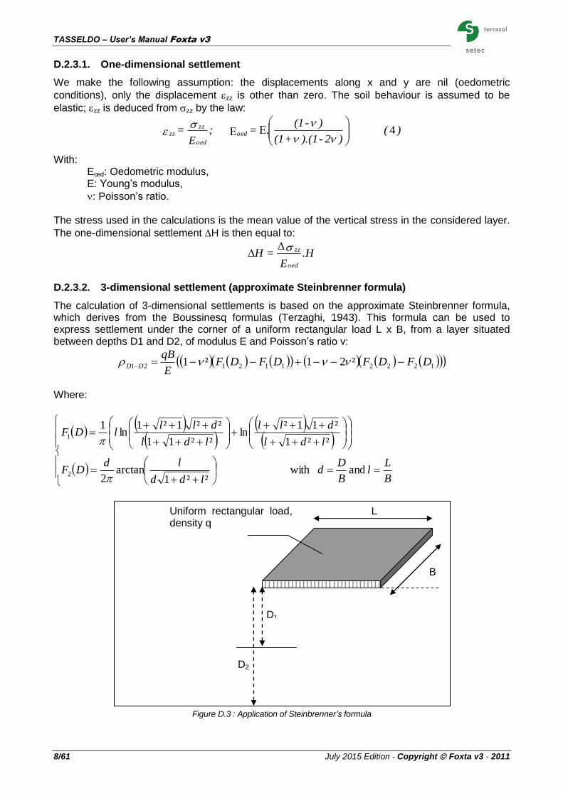
D.2.3.2. 3-dimensional settlement (approximate Steinbrenner formula)
The calculation of 3-dimensional settlements is based on the approximate Steinbrenner formula, which derives from the Boussinesq formulas (Terzaghi, 1943). This formula can be used to express settlement under the corner of a uniform rectangular load L x B, from a layer situated between depths D1 and D2, of modulus E and Poisson’s ratio ν:
1222112121 ²21²1 DFDFDFDFE
qBDD
Where:
B
Ll
B
Dd
ldd
ldDF
ldl
dll
ldl
dlllDF
and with ²²1
arctan2
²²1
²11²ln
²²11
²²1²1ln
1
2
1
Figure D.3 : Application of Steinbrenner’s formula
D1
Uniform rectangular load, density q
B
L
D2

TASSELDO – User’s Manual Foxta v3
Copyright Foxta v3 – 2011 – July 2015 Edition 9/61
D.2.3.3. Oedometric settlement
a) Final oedometric settlement
The oedometric settlement H is deduced from the oedometric curve (Figure D.4) representing the
void ratio as a function of the vertical effective stress 'v in the soil: e = f(zz'), characterised by: Cs: swelling ratio; Cc: consolidation ratio; eo: initial void ratio;
o': initial effective geostatic stress;
p': preconsolidation pressure;
tc: overconsolidation factor, by convention tc = p'/o' if tc > 0
tc = -(p'-o') if tc < 0 We assume that lateral displacements are nil (one-dimensional displacement assumption is valid) and that the volume of skeleton grains remains constant. The relationship between the variation in vertical displacement and that of the void ratio is defined by:
)e+(1
e=
H
H
oo
Figure D.4 : Void ratio e versus ’v
The oedometric settlement H due to a rise in the effective stress zz' (calculated) depends on the reference state and the soil loading history:
first case: normally consolidated soil: 0'=p', the oedometric settlement can be written:
if 'zz>0, (5) +
.e+1
CH.=H
o
zzo
10
o
c
log
if 'zz<0, (6) +
.e+1
CH.=H
o
zzo
10
o
s
log

TASSELDO – User’s Manual Foxta v3
10/61 July 2015 Edition - Copyright Foxta v3 - 2011
second case: overconsolidated soil: 0'< p'
If p'< 'zz+0' and zz'>0 (load case), oedometric settlement can be written:
(7) +
.C+.C.)e+(1
H=H
p
zzo
10c
o
p
10s
o
o
loglog
If p' > zz'+o' then settlement H can be deduced from formula (6). b) Settlement at time t
We can consider that in the overconsolidated domain, consolidation is far faster than in the normally consolidated domain.
Thus, for each layer, the degree of consolidation is only applied to the stress variation exceeding the consolidation pressure.
At a time t, we consider that the stress value is:
pspv tUt '''' 0
Us(t), provided layer by layer by the user, must be deduced from a prior consolidation calculation (to be carried out with specific software).
The additional stress at time t can be written:
0'' tt v
The value thus evaluated is input into whichever of formulas (5) to (7) is applicable.
D.2.4. Applications and limits
Application of the Boussinesq formulas for the semi-infinite, elastic, homogeneous, isotropic medium is acceptable as long as there are no significant differences in stiffness between the various layers. This is generally the case of soils subject to significant displacements. The case of a stiff layer on top of a soft layer cannot be dealt with in this way.
The elasticity displacements approach (1D or 3D calculation) requires a correct evaluation of the Young’s modulus for the stresses domain and the range of expected displacements under the structure. This is important in the case of granular soils in which the modulus increases with the
mean stress m and decreases with displacement.
The calculations performed generally show little difference between the 1D calculation and the 3D calculation.
Burland underlined that the oedometric approach for estimating total settlement under a foundation gave an order of magnitude at least equivalent to that given by the most sophisticated calculation methods, for all soils with approximate “elastic” behaviour under the effect of vertical loads.
The oedometric approach implicitly includes the variation in stiffness with the level of loading.
The degrees of consolidation introduced for the settlement calculation as a function of time must be deduced from a consolidation calculation representative of the conditions encountered (to be performed using specific software).

TASSELDO – User’s Manual Foxta v3
Copyright Foxta v3 – 2011 – July 2015 Edition 11/61
DD..33.. UUSSEERR’’SS MMAANNUUAALL
This chapter presents:
the Tasseldo module input parameters. Some zones can only take data with a physical meaning (for example, a Poisson’s ratio must always be strictly included between 0 and 0.5). The input window for the Tasseldo calculation parameters comprises 5 separate tabs. The data to be filled out in each tab sometimes depend on certain choices made by the user: for example, the data from to the oedometric calculation are only required if this type of calculation was requested by the user.
the results provided by the Tasseldo module. Here again, they partly depend on the data input by the user, in particular the type of calculation.
This chapter does not detail the actual user interface and its operations (buttons, menus, etc.): these aspects are dealt with in part C of the manual.
D.3.1. “Parameters” tab
Figure D.5 : “Parameters” tab
D.3.1.1. "General parameters” frame
This tab is used to define
the calculation title: maximum of 80 characters;
the level of printing detail: this is in fact the level of detail for generation of the formatted numerical results file (see chapter D.3.6.2.1).
D.3.1.2. “Import” frame
In the Tasseldo module, it is possible to import a project from the Tasplaq module.
In the context of a Tasplaq calculation, the Foxta software edits a .tso file, which is the format recognised by the Tasseldo module. This file can be imported into the Tasseldo module.

TASSELDO – User’s Manual Foxta v3
12/61 July 2015 Edition - Copyright Foxta v3 - 2011
In the “Parameters” tab, the button opens the “Tasseldo project
import wizard” which is used to select the directory containing the *[TQ].tso file from the Tasplaq project and then carry out the import operation:
“Import directory” frame: please, provide the path to the directory containing the Tasseldo project. By default, Foxta proposes the directory containing the current project. If
necessary, use the Browse button to select the relevant directory. Foxta could
display a warning message if the calculation date is a long time in the past and ask you to check the project data;
The names of the available Tasplaq projects appear in the left-hand frame: select one;
The corresponding calculation date appears on the right;
Information about data imported from the Tasplaq module appears in the right-hand frame.
Click the button to confirm data import or click .
Figure D.6 : Wizard for importing a Tasplaq file into the Tasseldo module
It is also possible to export the results of a Tasplaq calculation to the Tasseldo module. For more details, check the Tasplaq User’s Manual (part I).
D.3.2. “Layers” tab
This second tab is used to input parameters concerning soil behaviour.

TASSELDO – User’s Manual Foxta v3
Copyright Foxta v3 – 2011 – July 2015 Edition 13/61
Figure D.7 : “Layers” tab
Various information is accessible according to the type of calculation selected.
D.3.2.1. “Calculation type” frame
The choice of calculation type lets the user state whether he wants to perform an oedometric calculation in addition to the 3D and 1D Elastic calculation.
If “3D, 1D elastic and oedometric” calculation is selected:
The soil layers definition table contains additional columns;
The “Oedometric calculation parameters” frame appears;
The Consolidation" tab is activated.
Note: the combination of elastic and oedometric approaches can for example be useful for adjusting the elastic moduli of project layers with respect to oedometric settlement, or in the general case of a soil consisting of a succession of sands and clays.
D.3.2.2. “Soil layers definition” frame
This frame first requires the input of the top of the first soil layer that is the GL elevation (m). It must be higher than the base elevation of the first layer which will be defined in the soil layers definition table immediately below.
The choice of an oedometric calculation requires definition of an overconsolidation parameter ‘tc’ as follows:
if tc>0 then tc = 'p/v'0
if tc<0 then tc = - ('p - v'0)
Where v'0 is the initial vertical effective stress and ’p the pre-consolidation stress.

TASSELDO – User’s Manual Foxta v3
14/61 July 2015 Edition - Copyright Foxta v3 - 2011
The following table describes the soil properties to be defined for each layer:
Designation Unit Default value
Display condition
Mandatory value
Local checks
Z: elevation of layer base m
1 m below the base of the layer above
Always Yes Strictly decreasing values
E: Young’s modulus kPa - Always Yes > 0
: Poisson’s ratio - - Always Yes 0 < < 0.5
Cs/(1+e0): recompression (or swelling) ratio
- - Oedometric calculation
only
Yes if displayed
≥ 0
tc: overconsolidation parameter
- or
kPa -
Oedometric calculation
only
Yes if displayed
-
Cc/(1+e0): consolidation ratio
- - Oedometric calculation
only
Yes if displayed
≥ 0
: total unit weight of
layer (' is automatically taken into account if the layer is submerged,
always input )
kN/m3 -
Oedometric calculation
only
Yes if displayed
> 0
n: number of layer subdivisions (discretisation for the calculations)
- 1 Always Yes ≥ 1
Table D.1 : Soil layer parameters
Foxta can be used to save soil layers in the project soils database and/or in the global soils
database by clicking the button.
This saves the soil layers with their parameters and avoids having to input them again when creating a new module in the current project, or in another Foxta project.
Use of the soils database is described in detail in part C of the manual.
D.3.2.3. “Oedometric calculation parameters” frame
This frame, which is only visible if the user has chosen an oedometric calculation, is used to input the following:
Designation Unit Default value
Display condition
Mandatory value
Local checks
vo': vertical effective stress applied to the top of the first layer
kPa 0.00 Always Yes
≥ 0
Zw: groundwater level m 0.00 Always Yes -
w: unit weight of water kN/m3 10.00 Always Yes > 0
Table D.2 : Oedometric calculation parameters
TASSELDO – User’s Manual Foxta v3
Copyright Foxta v3 – 2011 – July 2015 Edition 15/61
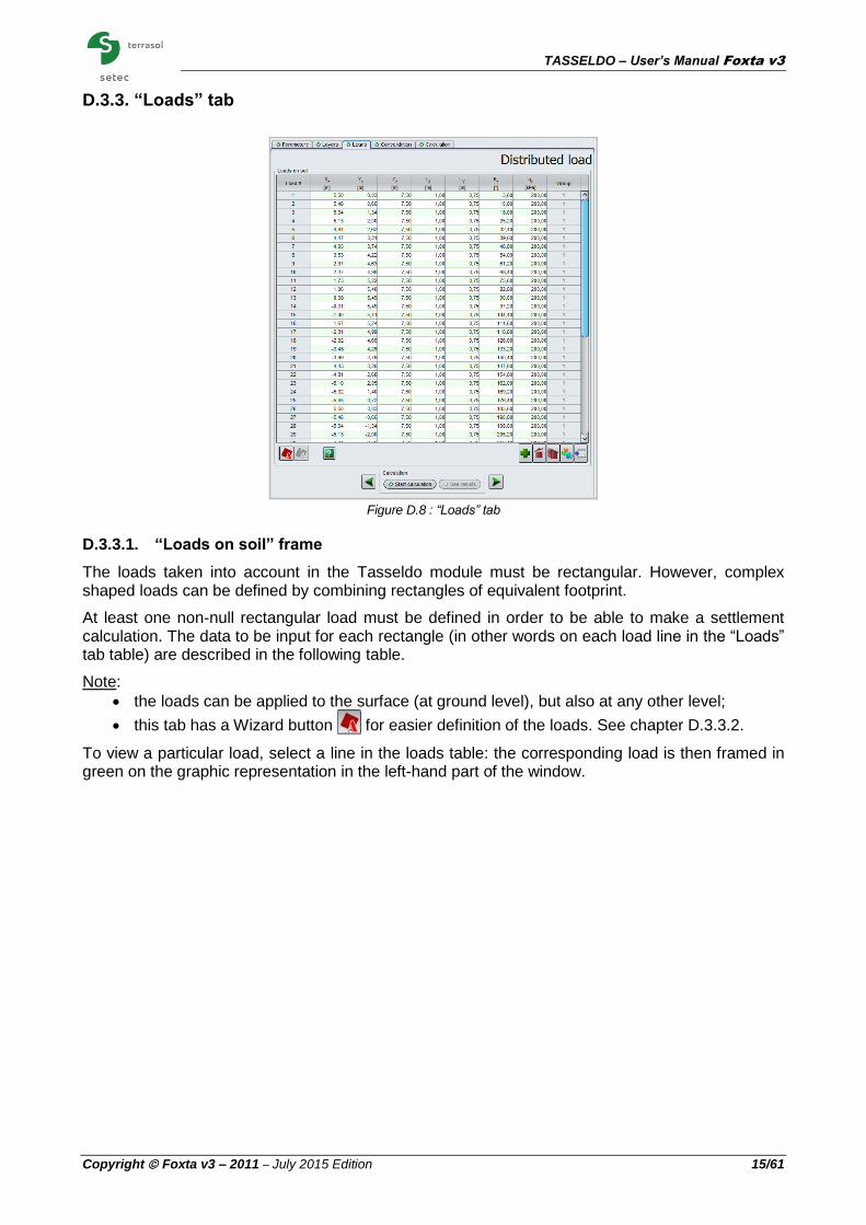
D.3.3. “Loads” tab
Figure D.8 : “Loads” tab
D.3.3.1. “Loads on soil” frame
The loads taken into account in the Tasseldo module must be rectangular. However, complex shaped loads can be defined by combining rectangles of equivalent footprint.
At least one non-null rectangular load must be defined in order to be able to make a settlement calculation. The data to be input for each rectangle (in other words on each load line in the “Loads” tab table) are described in the following table.
Note:
the loads can be applied to the surface (at ground level), but also at any other level;
this tab has a Wizard button for easier definition of the loads. See chapter D.3.3.2.
To view a particular load, select a line in the loads table: the corresponding load is then framed in green on the graphic representation in the left-hand part of the window.

TASSELDO – User’s Manual Foxta v3
16/61 July 2015 Edition - Copyright Foxta v3 - 2011
Designation Unit Default value
Display condition
Mandatory value
Local checks
Xr, Yr, Zr: Coordinates of the reference corner of the rectangle (Z axis upwards)
m - Always Yes
Lx, Ly: dimensions along local x and y axis of the rectangle
m - Always Yes
r: angle between side Lx and axis Ox (positive in the counter-clockwise direction)
° - Always Yes
qr: uniform load density kPa Always Yes ≠ 0
Group (a group of loads corresponds to a set of load rectangles generated with the wizard)
- -
If one of the “loads”
wizards was used
Filled out automatically
-
Table D.3 : Parameters for loads definition
Figure D.9 : View of a particular load

TASSELDO – User’s Manual Foxta v3
Copyright Foxta v3 – 2011 – July 2015 Edition 17/61
D.3.3.2. Loads wizard
To make the definition of “routine” loads easier, this tab has a Wizard button used for simple
definition of:
a uniform circular load;
a uniform annular load;
a 3D embankment type load.
Figure D.10 illustrates the various available wizards:
Choose the type of load;
Fill out the various input fields;
Click the button.
The use of the various load tabs is described in the following sub-chapters.
Note: it is possible to use several wizards or the same Loads wizard several times for the same Tasseldo calculation.
Figure D.10 : Automatic loads (wizards)
D.3.3.2.1. Wizard: "Uniform circular load"
This wizard is used to generate a group of rectangular loads equivalent to a uniform circular load.
The data to be input are as follows:
Designation Unit Default value
Display condition
Mandatory value
Local checks
Point A (XA, YA, ZA): coordinates of centre of loaded disk
m (0,0,0) Always Yes
Radius of loaded disk m - Always Yes >0
Subdivisions number - 10 Always Yes >0
Density of load kPa - Always Yes -
Table D.4 : Parameters for uniform circular load

TASSELDO – User’s Manual Foxta v3
18/61 July 2015 Edition - Copyright Foxta v3 - 2011
Figure D.11 : "Uniform circular load"
Generation of rectangular loads representing the circular load and calculation of their properties Xr,
Yr, Zr, LX, LY, r and qr, are activated by clicking the button:
Figure D.12 : Calculated values: "Uniform circular load"

TASSELDO – User’s Manual Foxta v3
Copyright Foxta v3 – 2011 – July 2015 Edition 19/61
D.3.3.2.2. Wizard: Uniform annular load
This wizard is used to generate a group of rectangular loads equivalent to a uniform annular load.
Figure D.13 : "Uniform annular load"
The data to be input are as follows:
Designation Unit Default value
Display condition
Mandatory value
Local checks
Point A (XA, YA, ZA): coordinates of centre of ring
m (0,0,0) Always Yes
Average radius of ring m - Always Yes > 0
Thickness of ring m - Always Yes > 0
Subdivisions number - 20 Always Yes > 0
Density of load kPa - Always Yes -
Table D.5 : Parameters for uniform annular load
TASSELDO – User’s Manual Foxta v3
20/61 July 2015 Edition - Copyright Foxta v3 - 2011
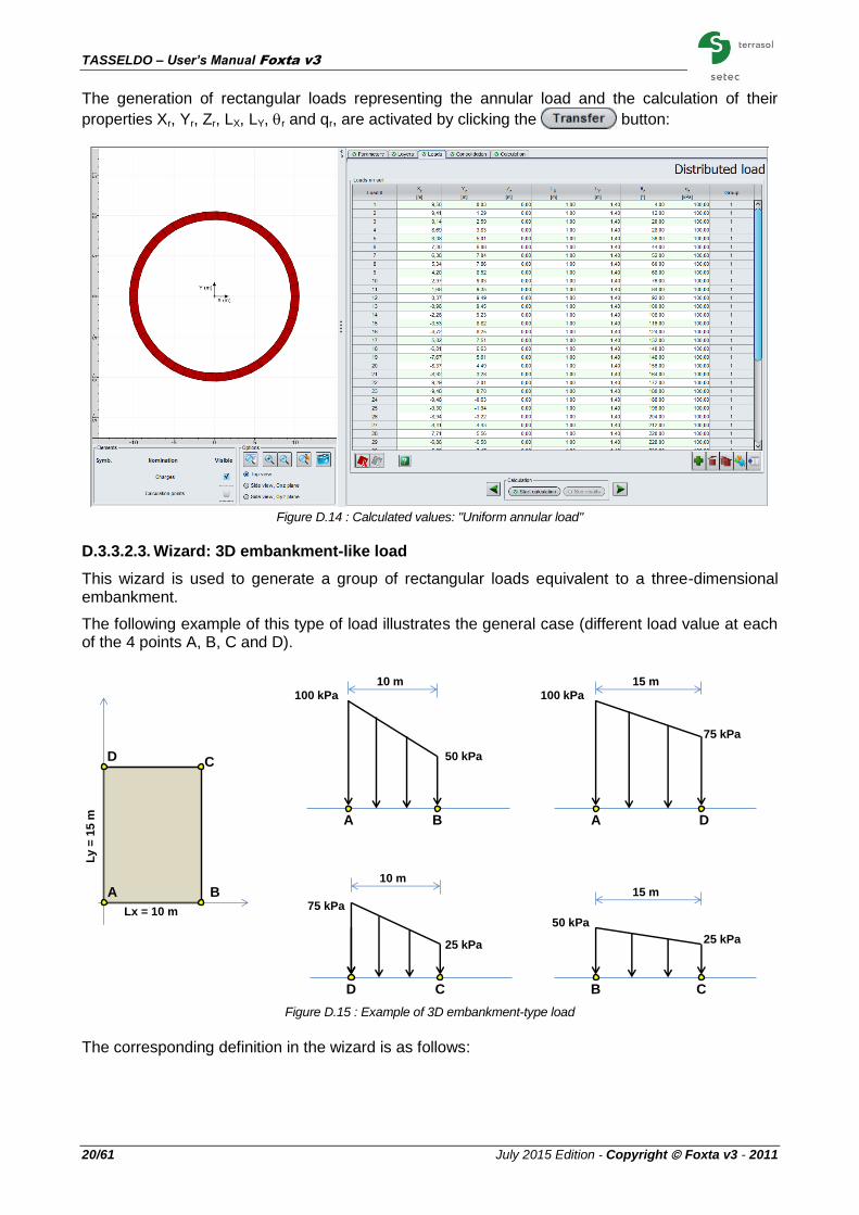
The generation of rectangular loads representing the annular load and the calculation of their
properties Xr, Yr, Zr, LX, LY, r and qr, are activated by clicking the button:
Figure D.14 : Calculated values: "Uniform annular load"
D.3.3.2.3. Wizard: 3D embankment-like load
This wizard is used to generate a group of rectangular loads equivalent to a three-dimensional embankment.
The following example of this type of load illustrates the general case (different load value at each of the 4 points A, B, C and D).
Lx = 10 m
Ly =
15
m
A
D C
B
A B
100 kPa
50 kPa
10 m
A D
100 kPa
75 kPa
B C
15 m
50 kPa
25 kPa
D C
10 m
75 kPa
25 kPa
15 m
Figure D.15 : Example of 3D embankment-type load
The corresponding definition in the wizard is as follows:
TASSELDO – User’s Manual Foxta v3
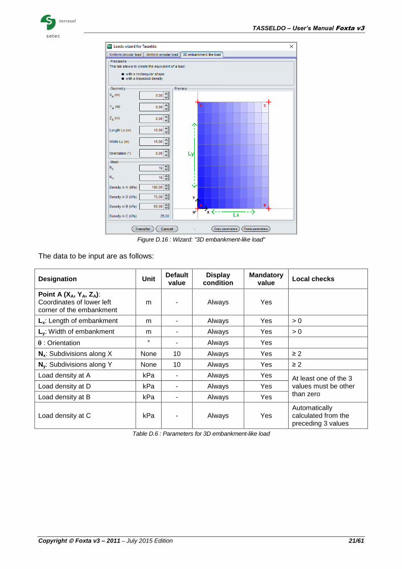
Copyright Foxta v3 – 2011 – July 2015 Edition 21/61
Figure D.16 : Wizard: "3D embankment-like load"
The data to be input are as follows:
Designation Unit Default value
Display condition
Mandatory value
Local checks
Point A (XA, YA, ZA): Coordinates of lower left corner of the embankment
m - Always Yes
Lx: Length of embankment m - Always Yes > 0
Ly: Width of embankment m - Always Yes > 0
: Orientation ° - Always Yes
Nx: Subdivisions along X None 10 Always Yes ≥ 2
Ny: Subdivisions along Y None 10 Always Yes ≥ 2
Load density at A kPa - Always Yes At least one of the 3 values must be other than zero
Load density at D kPa - Always Yes
Load density at B kPa - Always Yes
Load density at C kPa - Always Yes Automatically calculated from the preceding 3 values
Table D.6 : Parameters for 3D embankment-like load

TASSELDO – User’s Manual Foxta v3
22/61 July 2015 Edition - Copyright Foxta v3 - 2011
The generation of load rectangles representing the “3D embankment-like load” and the calculation
of their properties Xr, Yr, Zr, LX, LY, r and qr, are activated by clicking the button:
Figure D.17 : Calculated values: "3D embankment-like load"

TASSELDO – User’s Manual Foxta v3
Copyright Foxta v3 – 2011 – July 2015 Edition 23/61
D.3.4. "Consolidation" tab
This tab is only accessible if the "3D, 1D elastic and oedometric" option in the “Layers” tab has been selected.
To take account of consolidation in the context of an oedometric calculation, it is necessary first of all to check the “Consideration of consolidation” box and then input the required data in the 2 frames of the tab.
Figure D.18 : "Consolidation" tab
D.3.4.1. "Consolidation dates definition" frame
This frame is used to define the various consolidation dates (ascending) t1, t2, …ti, …t20 to be considered, in other words the dates for which the user is then required to define the consolidation percentage rate of each layer Xu(ti).
The dates are expressed without units (because they are not used in the calculations but only for display): it is therefore user’s responsibility to define dates that are consistent.
Adding a date ("+" button under the table) adds a column to the table.
D.3.4.2. “Consolidation rates by layer and by date” frame
This should be used to define the consolidation percentage of each layer, for each date defined above. The software automatically creates a line per layer in the table.
Value Xu(ti) = 100% corresponds to complete consolidation of the layer concerned on date ti.
The consolidation percentages input are allocated to the active layers base. When a layer is subdivided into several sub-layers, the program performs linear interpolation of the consolidations to allocate a consolidation percentage for each date that is consistent with the position of each sub-layer.
TASSELDO – User’s Manual Foxta v3
24/61 July 2015 Edition - Copyright Foxta v3 - 2011
The parameters to be filled out are:
Designation Unit Default value
Display condition
Mandatory value
Local checks
Xu(ti): consolidation rate of the layer indicated on date ti
% - Always Yes
0 ≤ Xu(ti) ≤ 100%
The values of Xu must be ascending (not strictly) over time within a given layer
Table D.7 : Consolidation parameters
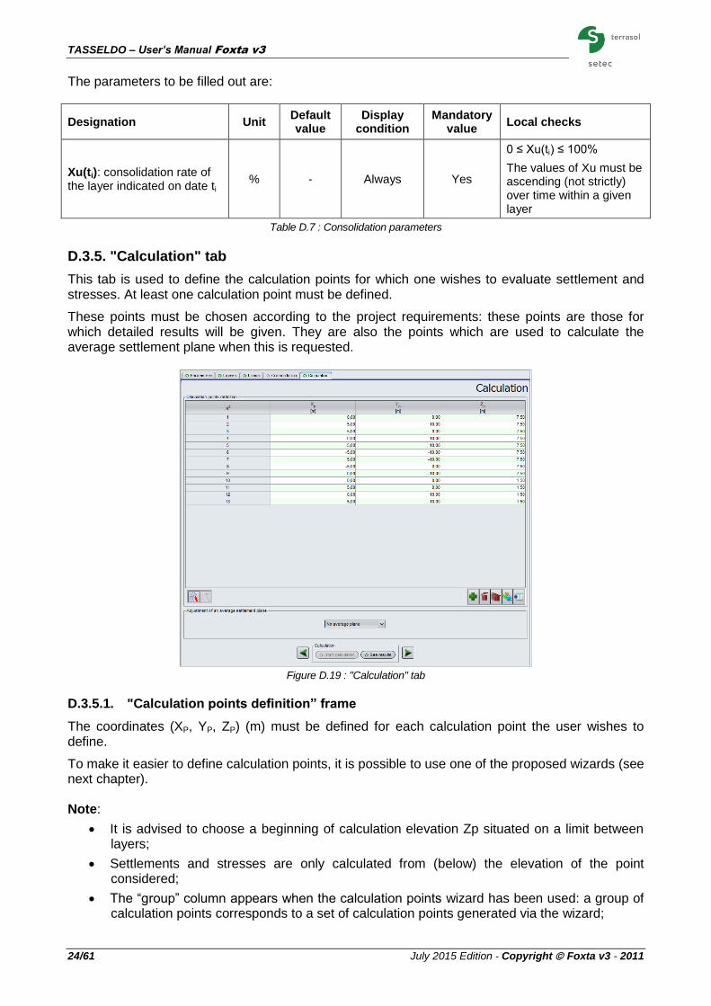
D.3.5. "Calculation" tab
This tab is used to define the calculation points for which one wishes to evaluate settlement and stresses. At least one calculation point must be defined.
These points must be chosen according to the project requirements: these points are those for which detailed results will be given. They are also the points which are used to calculate the average settlement plane when this is requested.
Figure D.19 : "Calculation" tab
D.3.5.1. "Calculation points definition” frame
The coordinates (XP, YP, ZP) (m) must be defined for each calculation point the user wishes to define.
To make it easier to define calculation points, it is possible to use one of the proposed wizards (see next chapter). Note:
It is advised to choose a beginning of calculation elevation Zp situated on a limit between layers;
Settlements and stresses are only calculated from (below) the elevation of the point considered;
The “group” column appears when the calculation points wizard has been used: a group of calculation points corresponds to a set of calculation points generated via the wizard;

TASSELDO – User’s Manual Foxta v3
Copyright Foxta v3 – 2011 – July 2015 Edition 25/61
The application marks the point selected in the table with a green cross in the graphic part:
Figure D.20 : Selection of a calculation point – Graphic representation
Note: the view presented by default in the graphic space is the project top view. Using the
and buttons, it is also possible to display the side view (planes
Oyz or Oxz).
These views can for example be used to visualise load and calculation points defined at depth.
Figure D.21 : Example of graphic representation of side view (Oyz plane)

TASSELDO – User’s Manual Foxta v3
26/61 July 2015 Edition - Copyright Foxta v3 - 2011
D.3.5.2. Calculation points wizards
These wizards are used to automatically generate aligned points or points distributed according to
predetermined geometries. They are accessible by clicking the button.
Several wizards can be used or the same wizard can be used several times in the same Tasseldo calculation.
After using at least one “Calculation points” wizard, the button becomes accessible: it is used
to modify the selected group of calculation points.
D.3.5.2.1. Calculation points situated along a segment
This wizard is used to automatically generate calculation points aligned along a segment [A, B].
Figure D.22 : Calculation points situated along a segment
The following parameters are to be filled out:
Designation Unit Default value
Display condition
Mandatory value
Local checks
Point A (XA, YA, ZA): Coordinates of point A
m - Always Yes The 2 points must be distinct Point B (XB, YB, ZB):
Coordinates of point B m - Always Yes
Number of points - 10 Always Yes ≥ 2
Table D.8 : Parameters for defining calculation points situated along a segment
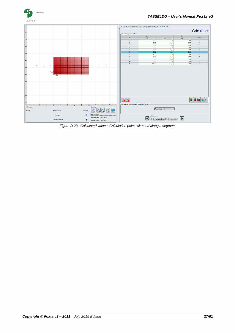
Once the wizard data have been completed, click the button: the points generated are
then automatically copied into the table of calculation points in the “Calculation” tab:
TASSELDO – User’s Manual Foxta v3
Copyright Foxta v3 – 2011 – July 2015 Edition 27/61
Figure D.23 : Calculated values: Calculation points situated along a segment

TASSELDO – User’s Manual Foxta v3
28/61 July 2015 Edition - Copyright Foxta v3 - 2011
D.3.5.2.2. Calculation points situated along a horizontal circle
This wizard is used to automatically define calculation points aligned along a circle with centre A.
Figure D.24 : Calculation points situated along a horizontal circle
The parameters to be filled out are as follows:
Designation Unit Default value
Display condition
Mandatory value
Local checks
Point A (XA, YA, ZA) m - Always Yes
Radius of circle m - Always Yes > 0
Number of points - 10 Always Yes ≥ 2
Table D.9 : Parameters for definition of calculation points situated along a horizontal circle
Once the wizard data have been completed, click the button: the points generated are
then automatically copied into the calculation points table in the “Calculation” tab:
Figure D.25 : Calculated values: Calculation points situated along a horizontal circle

TASSELDO – User’s Manual Foxta v3
Copyright Foxta v3 – 2011 – July 2015 Edition 29/61
D.3.5.2.3. Calculation points distributed on a horizontal rectangle
This wizard is used to automatically define a mesh of calculation points distributed on a horizontal rectangle [A, B, C, D].
Figure D.26 : Calculation points distributed on a horizontal rectangle
The following parameters are to be filled out:
Designation Unit Default value
Display condition
Mandatory value
Local checks
Point A (XA, YA, ZA) m - Always Yes -
Lx: length of rectangle m - Always Yes > 0
Ly: width of rectangle m - Always Yes > 0
Number of points along Lx - 7 Always Yes ≥ 2
Number of points along Ly - 7 Always Yes ≥ 2
Table D.10 : Parameters for definition of calculation points distributed on a horizontal rectangle
Once the wizard data have been completed, click the button: the generated points are
then automatically copied into the calculation points table in the "Calculation" tab:
Figure D.27 : Calculated values: Calculation points distributed on a horizontal rectangle
TASSELDO – User’s Manual Foxta v3
30/61 July 2015 Edition - Copyright Foxta v3 - 2011
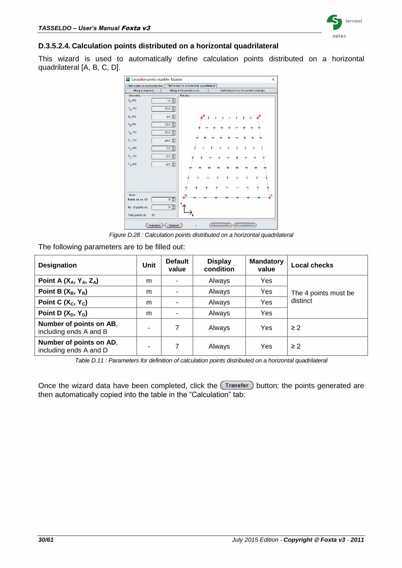
D.3.5.2.4. Calculation points distributed on a horizontal quadrilateral
This wizard is used to automatically define calculation points distributed on a horizontal quadrilateral [A, B, C, D].
Figure D.28 : Calculation points distributed on a horizontal quadrilateral
The following parameters are to be filled out:
Designation Unit Default value
Display condition
Mandatory value
Local checks
Point A (XA, YA, ZA) m - Always Yes
The 4 points must be distinct
Point B (XB, YB) m - Always Yes
Point C (XC, YC) m - Always Yes
Point D (XD, YD) m - Always Yes
Number of points on AB, including ends A and B
- 7 Always Yes ≥ 2
Number of points on AD, including ends A and D
- 7 Always Yes ≥ 2
Table D.11 : Parameters for definition of calculation points distributed on a horizontal quadrilateral
Once the wizard data have been completed, click the button: the points generated are
then automatically copied into the table in the “Calculation” tab:

TASSELDO – User’s Manual Foxta v3
Copyright Foxta v3 – 2011 – July 2015 Edition 31/61
Figure D.29 : Calculated values: Calculation points distributed on a horizontal quadrilateral
D.3.5.2.5. Calculation points distributed on a horizontal disk
This wizard is used to automatically define calculation points distributed on a disk with centre A.
Figure D.30 : Calculation points distributed on a horizontal disk
The following parameters are to be filled out:
Designation Unit Default value
Display condition
Mandatory value
Local checks
Point A (XA, YA, ZA) m - Always Yes
Radius of disk m - Always Yes > 0
Nr: number of radial subdivisions (number of circles)
- 5 Always Yes ≥ 1
Nnumber of orthoradial subdivisions (number of points on each circle)
- 10 Always Yes ≥ 2
Table D.12 : Parameters for definition of calculation points distributed on a horizontal disk

TASSELDO – User’s Manual Foxta v3
32/61 July 2015 Edition - Copyright Foxta v3 - 2011
Once the wizard data have been completed, click the button: the points generated are
then automatically copied into the calculation points table in the "Calculation" tab:
Figure D.31 : Calculated values: Calculation points situated on a horizontal disk
D.3.5.3. Adjustment of an average settlement plane
The drop-down list may be used to request calculation of an average settlement plane by selecting the appropriate choice. The possible choices are as follows:
No average plane;
1D average plane: calculation of average plane on the basis of 1D elastic settlement and the defined calculation points;
3D average plane: calculation of average plane on the basis of 3D elastic settlement and the defined calculation points;
Oedo average plane: calculation of average plane on the basis of oedometric settlement and the calculation points defined.
D.3.6. Calculation and results
D.3.6.1. Calculation
The calculation can be started from any tab, provided that the tabs have been correctly filled out, in
other words when they are all marked with a green cross (for example: ).
They are marked with a red cross (for example: ) until they are correctly filled out (data
missing or not conforming to expected values).
To start the calculation, click the button.
D.3.6.2. Results
To display the calculation results, click the button.
The following window then appears and proposes the different types of results accessible after a Tasseldo calculation:

TASSELDO – User’s Manual Foxta v3
Copyright Foxta v3 – 2011 – July 2015 Edition 33/61
Figure D.32 : Numerical and graphical results
3 types of numerical results: formatted results, stresses and settlements, and consolidation settlements (oedometric);
3 types of graphical results: stresses and settlements, consolidation settlements (oedometric) and settlement shadings.
Click the required button according to the data format.
The following chapters describe these different types of results in detail.
D.3.6.2.1. Formatted numerical results
This window contains a summary of the calculation data and results:
Figure D.33 : Numerical results: Formatted results – Data reminder

TASSELDO – User’s Manual Foxta v3
34/61 July 2015 Edition - Copyright Foxta v3 - 2011
The formatted results contain:
A reminder of the data (Figure D.33): general parameters, soil data, loads, etc. This section
also includes a table giving the effective stresses '0 and 'p in the centre of each sub-layer (taking account of discretisation of the layers for definition of the sub-layers);
Results in normal printing mode:
The summary table of results for the various calculation points (Figure D.34):
Coordinates (X, Y, Z) of calculation point (m)
T1d: value of 1D elastic settlement calculated for this point
T3d: value of 3D elastic settlement calculated for this point
Toedo: value of oedometric settlement calculated (only if oedometric calculation had been requested. If not, the column comprises only nil values).
Note: positive settlement values correspond to actual settlements (downwards). Negative values correspond to heaving.
Figure D.34 : Numerical results: Formatted results – Results (normal printing)
Or results in detailed printing mode:
A table of results for each calculation point (Figure D.35):
Calculation level (m)
Vertical stress at mid-thickness of the (sub-)layer
T1d: value of 1D elastic settlement calculated for this point
T3d: value of 3D elastic settlement calculated for this point
Toedo: value of oedometric settlement calculated for this point (only if oedometric calculation had been requested. If not, the column comprises only nil values).
This results display mode can in particular be used to easily check the contribution of a layer to settlement at a given point.
Note: in the same way as above, positive settlement values correspond to actual settlement (downwards), while negative values correspond to heaving.
The average plane, if requested (Figure D.36). This section:
Gives the equation of the calculated average plane;
Recalls the coordinates (XP, YP) of each calculation point;

TASSELDO – User’s Manual Foxta v3
Copyright Foxta v3 – 2011 – July 2015 Edition 35/61
In the “calculated” column, for each calculation point, recalls the calculated settlement using the calculation method adopted for the average plane (display of 3D elastic settlement if the 3D elastic average plane was requested, for example);
In the “adjusted” column, gives the settlement value, at the same calculation point, corresponding to the position of the settlement average plane.
Figure D.35 : Numerical results: Formatted results (detailed printing)

TASSELDO – User’s Manual Foxta v3
36/61 July 2015 Edition - Copyright Foxta v3 - 2011
Figure D.36 : Numerical results: Formatted results – Results (adjusted plane)
D.3.6.2.2. Numerical results – Stresses and Settlements
This table contains the stresses and settlements at the calculation points, as a function of the elevation Z (m):
Designation Unit Display condition
N° calculation point (point coordinates) - Always
Z: elevation m Always
V: Supplementary vertical stress kPa Always
1D Settlement: one-dimensional elastic settlement m Always
3D Settlement: three-dimensional elastic settlement m Always
Oedo(metric) Settlement m Only if oedometric calculation was requested
Table D.13 : Details of numerical results (stresses and settlements)

TASSELDO – User’s Manual Foxta v3
Copyright Foxta v3 – 2011 – July 2015 Edition 37/61
Figure D.37 : Numerical results: Stresses and settlements
D.3.6.2.3. Numerical results – Consolidation settlement (oedometric)
The table only contains results if an oedometric calculation with consolidation has been carried out.
Figure D.38 : Numerical results: Consolidation settlements (oedometric)
Designation Unit Display condition
N° calculation point (coordinates of point) - Always
Date ti: consolidation dates (as input in the data) - Always
Oedo settlement: oedometric settlement on the date considered (as a function of the consolidation rates of the various layers)
m Always
Table D.14 : Details of numerical results: Consolidation settlements (oedometric)

TASSELDO – User’s Manual Foxta v3
38/61 July 2015 Edition - Copyright Foxta v3 - 2011
D.3.6.2.4. Graphical results – Stresses and settlements
The curves present the same results as those described in the corresponding table (numerical results, chapter D.3.6.2.2).
It is possible to select/deselect several calculation points in the left-hand list: the curves corresponding to the selected points are then superposed over the graphics. The “Shift” key on the keyboard should be used to select several points.
Figure D.39 : Graphical results: Stresses and settlements
D.3.6.2.5. Graphical results - Consolidation settlements (oedometric)
The curves show the same results as those described in the corresponding table (numerical results, chapter D.3.6.2.3).
Here again, it is possible to select/deselect several calculation points in the left-hand list: the curves corresponding to the selected points are then superposed over the graphic.
Figure D.40 : Graphical results: Oedometric consolidation settlement

TASSELDO – User’s Manual Foxta v3
Copyright Foxta v3 – 2011 – July 2015 Edition 39/61
D.3.6.2.6. Graphical results – Settlements shadings
Figure D.41 : Graphical results : Settlements at given Z
This window can be used to show the settlement intensity for a given level Z. The following can be selected in the strip at the top of the window:
The chosen level
The type of settlement to be displayed: Elastic 1D, Elastic 3D or Oedometric (if available). In the example presented above, the colours illustrate the distribution of 1D elastic settlement values in plane (OXY) at elevation Z = 0.00.

TASSELDO – User’s Manual Foxta v3
40/61 July 2015 Edition - Copyright Foxta v3 - 2011
DD..44.. CCAALLCCUULLAATTIIOONN EEXXAAMMPPLLEESS
D.4.1. Example 1
D.4.1.1. Introduction
The first example comprises two parts:
Calculation of one-dimensional and three-dimensional settlement of three soil layers under the effect of a rectangular load
Then calculation of the oedometric settlement in the same conditions.
D.4.1.2. Data input
At opening of the application, Foxta proposes:
creating a new project;
opening an existing project;
automatically opening the last project used.
In the case of this example:
choose to create a new project by selecting the radio-button;
click the button.
D.4.1.2.1. New project wizard: New project
“File” frame
Fill out the project path by clicking the button;
Give a name to the file and save it.
q = 50 kPa
Layer 1
Layer 2
Layer 3

TASSELDO – User’s Manual Foxta v3
Copyright Foxta v3 – 2011 – July 2015 Edition 41/61
“Project” frame
Give a title to the project;
Enter a project number;
Complete with comments if necessary;
Leave the “Use the soil database” unticked (we will not use the database for this example), and
click the button.
D.4.1.2.2. New project wizard: Choice of modules
In the “Modules” window, select the Tasseldo module then click the button.
The Tasseldo window appears.
The various data tabs proposed should be filled out.
D.4.1.2.3. Parameters tab
This tab contains two frames: “General parameters” tab:
Tasseldo calculation title: for this example, we will for example enter "Example 1";
Type of printing (normal or detailed): for this example, normal printing will be sufficient. “Import” frame:
A project can be imported from the Tasplaq module, but we will not use this option for this example.

TASSELDO – User’s Manual Foxta v3
42/61 July 2015 Edition - Copyright Foxta v3 - 2011
To move onto the next tab, click either the name of the “Layers” tab or the button.
D.4.1.2.4. “Layers” tab
This tab concerns the definition of soil layers.
“Calculation type” frame:
Retain the default choice “3D and 1D elastic”.

TASSELDO – User’s Manual Foxta v3
Copyright Foxta v3 – 2011 – July 2015 Edition 43/61
“Soil layers definition” frame:
Define the top of the first layer at level 7.50 m.
Then create three soil layers by clicking the button to add each of the layers.
The data to be input are as follows:
Name Zbase (m) Esoil (kPa) n
Layer 1 1.5 8000 0.33 10
Layer 2 -5.0 4000 0.33 10
Layer 3 -15 20000 0.33 10
Note: the discretisation chosen makes it possible here to create “sub-layers” from 50 cm to one metre thick.
The drawing in the left-hand part of the screen shows the layers defined.
Tasseldo can be used to save these soil layers in the project database and/or in the global soils
database by clicking the button.
This makes it possible to save soil layers with their parameters, to avoid having to input them again when using another module for the same Foxta project, or when creating another Foxta project.
The database will not be used in this example, but part C of the manual describes its use in detail. “Oedometric calculation parameters":
This is not accessible here because in this first part we simply deal with elastic calculations (see choice of calculation type above).
D.4.1.2.5. “Loads” tab

TASSELDO – User’s Manual Foxta v3
44/61 July 2015 Edition - Copyright Foxta v3 - 2011
“Loads on soil” frame:
This “Loads” tab is used to define the loads applied at groundlevel. Here we use a single simple rectangle with the following characteristics:
Xr (m) Yr (m) Zr (m) Lx (m) Ly (m) r (°) qr (kPa)
0.00 0.00 7.50 10 20 0 50
Click the button to add a line and input the above values.
Note: in the examples covered in the manual, the loads are always applied at surface level. However, it should be noted that it is also possible to define loads at depth.
A help diagram can be accessed by clicking the button and illustrates the meaning of
parameters Lx, Ly and r:
The “Loads wizard” is not used in this example because the load only consists of a simple
rectangle. This wizard will be used in example 2.
The drawing in the left-hand part of the screen now shows the defined load.
D.4.1.2.6. "Consolidation" tab
This tab is not accessible here: it is only available in the case of an oedometric calculation.
D.4.1.2.7. "Calculation" tab
This tab is used to define the points for calculation of settlement.
These points must be chosen depending on the requirements of the project: these points are those for which detailed results will be provided. They are also the points which are used to calculate the average settlement plane when this is requested (this is not the case in this example).
Here we have chosen points on the surface and at a depth of 2 m, both under the applied load (under one quarter of the foundation, representative of the whole, owing to the symmetry of the project) and outside it (1 point defined outside the load footprint).

TASSELDO – User’s Manual Foxta v3
Copyright Foxta v3 – 2011 – July 2015 Edition 45/61
"Calculation points definition" frame:
Click the button to add a line and repeat this operation for all the points to be defined.
Note: here we define the calculation points manually. Use of the "Calculation points" wizard will be illustrated in example 2.
After defining these points, they appear in the left-hand part of the window as blue points (the point corresponding to the line selected in the table appears as a green cross).
N° Xp (m) Yp (m) Zp (m)
1 0.00 0.00 7.50
2 5.00 10.00 7.50
3 5.00 0.00 7.50
4 0.00 10.00 7.50
5 -5.00 10.00 7.50
6 -5.00 -10.00 7.50
7 5.00 -10.00 7.50
8 -5.00 0.00 7.50
9 0.00 -10.00 7.50
10 0.00 0.00 1.50
11 5.00 0.00 1.50
12 0.00 10.00 1.50
13 5.00 10.00 1.50
"Adjustment of an average settlement plane" frame:
We will not use an average plane for this example
Data input for this example is now completed.
D.4.1.3. Calculation and results
D.4.1.3.1. Calculation
As long as all the tabs have not been correctly filled out, the button used to start the calculation is
marked with a red cross: .

TASSELDO – User’s Manual Foxta v3
46/61 July 2015 Edition - Copyright Foxta v3 - 2011
Once all the data have been correctly input, the button (accessible from all the
tabs) is active.
Clicking this button will start the calculation.
To access the results in the form of tables and graphics, click the button.
“Numerical results” frame:
“Formatted results” and “Stresses and settlements” are accessible by clicking the corresponding button.
The “Consolidation settlements (oedometric)" results are not accessible because the "3D, 1D elastic (oedometric)" option was not selected for this example.
"Graphical results" frame:
The “Stresses and settlements” and “Settlements shadings” results are accessible by clicking the corresponding button.
The “Consolidation settlements (oedometric)" results are not accessible because the "3D, 1D elastic (oedometric)" option was not selected for this example.
D.4.1.3.2. Results
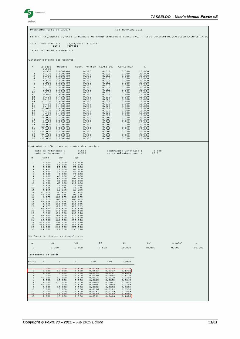
The main available results (in particular the settlements for the 9 calculation points) are presented on the following page.
The results given in terms of settlements are the 1D and 3D elastic settlements. The oedometric results are not available because the oedometric calculation was not requested for this example.
Select a type of results to be displayed then click the button to return to the result
types selection screen.
It should be noted that for each elevation (7.5 or 1.5), maximum settlement is obtained as planned in the centre of the loaded zone (points 2 and 13). Maximum settlement obtained on the surface is thus at point 2, with a value of 7.07 cm for 3D elastic settlement at this point. Settlement at point 13 (also at the centre of the loaded zone, but at elevation 1.5 m) is of 4.64 cm.
As oedometric calculation was not selected, the Toedo column is displayed, but contains only nil values.
To quit the results display, click the button.
Results not accessible for this example

TASSELDO – User’s Manual Foxta v3
Copyright Foxta v3 – 2011 – July 2015 Edition 47/61
Numerical results – Formatted results

TASSELDO – User’s Manual Foxta v3
48/61 July 2015 Edition - Copyright Foxta v3 - 2011
Numerical results – Stresses and settlements
Graphical results – Stresses and settlements

TASSELDO – User’s Manual Foxta v3
Copyright Foxta v3 – 2011 – July 2015 Edition 49/61
Graphical results – Settlements shading
D.4.1.3.3. Data modification
If necessary, it is possible to modify the data input in the same file and restart the calculation.
For example we here wish to supplement the previous calculation with the oedometric settlement
calculation: click the button, then the button to return to data
input. Then select the “Layers” tab, tick the “3D, 1D elastic and oedometric" option and fill out:
the new columns displayed in the soil characteristics table;
the “Oedometric calculation parameters” frame at the bottom of the same tab;
the "Consolidation" tab, which is now accessible: however we will not use this feature for this example. It will be illustrated in example 2.

TASSELDO – User’s Manual Foxta v3
50/61 July 2015 Edition - Copyright Foxta v3 - 2011
“Soil layers definition” frame:
The values to be input for the oedometric calculation are as follows:
Name Cs/(1+e0) tc Cc/(1+e0) (kN/m3)
Layer 1 0.012 -50 (kPa) 0.080 20.00
Layer 2 0.025 1.00 0.200 19.00
Layer 3 0.005 1.30 0.030 20.00
Note on the values of tc:
when positive: they correspond by convention to overconsolidation ratios (OCR). See chapter D.3.2.2.
when negative, they correspond by convention to overconsolidation pressures (in kPa). See chapter D.3.2.2.
“Oedometric calculation parameters” frame:
The additional values to be input are as follows:
vo' (kPa) Zw (m) w (kN/m3)
0.00 6.50 10.00
"Consolidation" tab:
Do not tick the “Consideration of consolidation" box (this feature will be illustrated in example 2).
Save the project under another name (TASSEL01bis for example) and restart the calculation. For analysis of the results, use the same method as before.
The numerical and graphical results of “Consolidation settlements (oedometric)" are still not always accessible: this is because although we activated oedometric calculation, the “Consolidation” feature for calculation of settlements with time is not used. Formatted numerical results:
Logically, the T1d and T3d settlements are exactly the same as for the 1st calculation (the data concerning the elastic calculation were not modified).
This time we also obtain the calculated values for oedometric settlement (column Toedo): these are far greater than the values resulting from the 2 elastic calculations: maximum oedometric settlement (point 2) of 17.0 cm instead of 7.07 cm for the same point with 3D elastic settlement.
If necessary, the comparison between these elastic and oedometric values enable the elastic modulus to be fitted with the oedometric characteristics of each soil layer.
TASSELDO – User’s Manual Foxta v3
Copyright Foxta v3 – 2011 – July 2015 Edition 51/61

TASSELDO – User’s Manual Foxta v3
52/61 July 2015 Edition - Copyright Foxta v3 - 2011
Graphical curves: Stresses and settlements
Maximum surface settlement is indeed at point 2 (17.0 cm for oedometric settlement and 7.1 cm for 3D elastic settlement.
For points outside the footprint of the loaded zone, the v term is nil on the surface and increases with depth.
Note:
Move the mouse over a curve to obtain the values corresponding to the points on the curve;
The settlement curves for the calculation points situated at elevation 1.5 m are extended vertically between levels 1.5 and 7.5 m (no settlement calculated above the calculation point).
___: calculation point N°1
___: calculation point N°2
___: calculation point N°10
___: calculation point N°13
TASSELDO – User’s Manual Foxta v3
Copyright Foxta v3 – 2011 – July 2015 Edition 53/61
D.4.2. Example 2
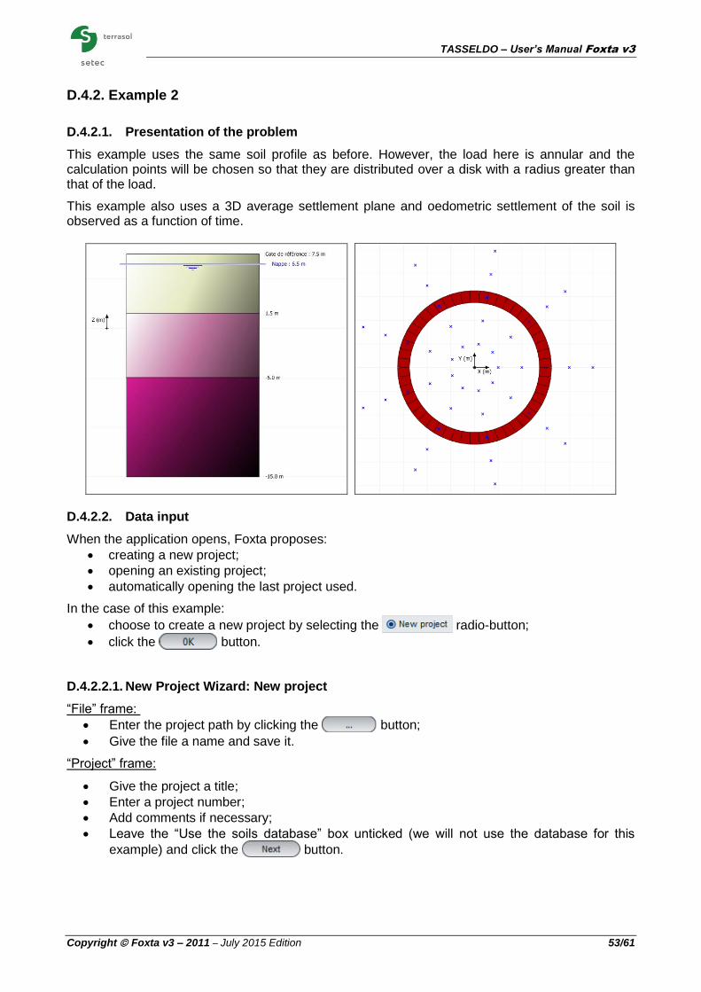
D.4.2.1. Presentation of the problem
This example uses the same soil profile as before. However, the load here is annular and the calculation points will be chosen so that they are distributed over a disk with a radius greater than that of the load.
This example also uses a 3D average settlement plane and oedometric settlement of the soil is observed as a function of time.
D.4.2.2. Data input
When the application opens, Foxta proposes:
creating a new project;
opening an existing project;
automatically opening the last project used.
In the case of this example:
choose to create a new project by selecting the radio-button;
click the button.
D.4.2.2.1. New Project Wizard: New project
“File” frame:
Enter the project path by clicking the button;
Give the file a name and save it.
“Project” frame:
Give the project a title;
Enter a project number;
Add comments if necessary;
Leave the “Use the soils database” box unticked (we will not use the database for this
example) and click the button.

TASSELDO – User’s Manual Foxta v3
54/61 July 2015 Edition - Copyright Foxta v3 - 2011
D.4.2.2.2. New Project Wizard: Choice of modules
In the “Modules” window, select the Tasseldo module then click the button.
The Tasseldo window appears.
The various data tabs proposed must be filled out.
D.4.2.2.3. “Parameters” tab
Apart from the project title, the first tab is filled out in the same way as for example 1.
D.4.2.2.4. “Layers” tab
“Calculation type” frame:
This time the “3D, 1D elastic and oedometric” option is ticked directly. “Soil layers definition” frame:
The following data are to be input (the same as for example 1: it is possible to go back to example 1, export soil layers to the general database and then import them when creating example 2, to avoid having to re-enter the same data. See part C of the manual):
Top of first layer: 7.50 m.
Name Zbase (m) Esoil
(kPa) Cs/(1+e0) tc Cc/(1+e0) (kN/m
3) n
Layer 1 1.50 8000 0.33 0.012 -50 (kPa) 0.08 20.00 10
Layer 2 -5 4000 0.33 0.025 1.00 0.20 19.00 10
Layer 3 -15 20000 0.33 0.005 1.30 0.03 20.00 10

TASSELDO – User’s Manual Foxta v3
Copyright Foxta v3 – 2011 – July 2015 Edition 55/61
“Oedometric calculation parameters” frame:
The following data are to be input:
vo' (kPa) Zw (m) w (kN/m3)
0.00 6.50 10.00
D.4.2.2.5. “Loads” tab
In the “Loads” tab, use the "Load Wizard" button (bottom-left of tab) and select the “Uniform
annular load” tab.

TASSELDO – User’s Manual Foxta v3
56/61 July 2015 Edition - Copyright Foxta v3 - 2011
The following data are to be input:
XA (m) YA (m) ZA (m) R (m) e (m) Subdivisions q (kPa)
0.00 0.00 7.50 6.00 1.00 50 200.00
The radius to be input is the average radius of the ring. In the case of this example, the inside radius of the ring is 5.5 m and the outside radius is 6.5 m.
Once the data are input, click the button to create the corresponding load rectangles in
the loads table: it is possible to check that the wizard has actually generated 50 rectangles to represent the ring. The rectangle selected from the list is surrounded by a green frame on the drawing.
D.4.2.2.6. "Consolidation" tab
Tick the “Consideration of consolidation” box and then fill out the tab: "Consolidation dates definition" frame:
To add date values (that is columns in the table), click the button.
The values to be input are as follows:
t1 t2 t3 t4
1 5 20 50

TASSELDO – User’s Manual Foxta v3
Copyright Foxta v3 – 2011 – July 2015 Edition 57/61
“Consolidation rates by layer and by date” frame:
3 lines corresponding to the 3 soil layers were automatically created.
For the three soil layers, their respective degrees of consolidation must be defined, expressed as a percentage, as a function of the dates. The values to be input for this example are as follows:
Layers Xu (t1) (%) Xu (t2) (%) Xu (t3) (%) Xu (t4) (%)
Layer 1 70 99 100 100
Layer 2 20 50 90 100
Layer 3 90 99 100 100
D.4.2.2.7. "Calculation" tab
It is now possible to generate the calculation points on the surface of a disk. “Calculation points definition" frame:
These points will be those used to calculate the average settlement plane. It is therefore important to select points that are distributed uniformly and symmetrically with respect to the loaded zone, in order to obtain a representative average plane (use of the wizard guarantees this homogeneous distribution of points in the defined zone).
TASSELDO – User’s Manual Foxta v3
58/61 July 2015 Edition - Copyright Foxta v3 - 2011
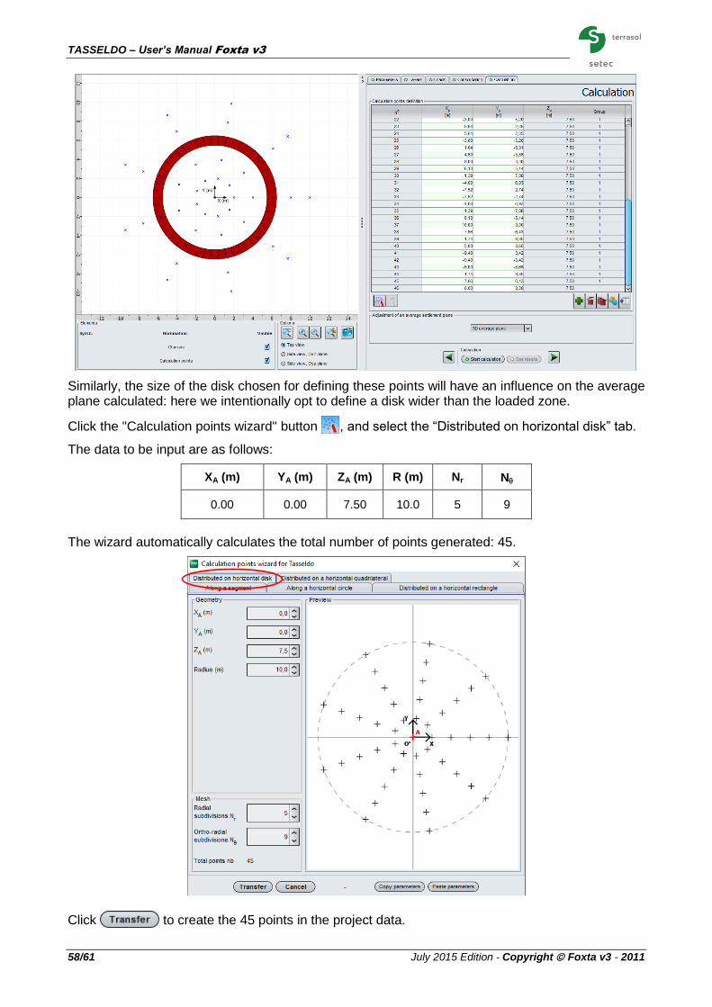
Similarly, the size of the disk chosen for defining these points will have an influence on the average plane calculated: here we intentionally opt to define a disk wider than the loaded zone.
Click the "Calculation points wizard" button , and select the “Distributed on horizontal disk” tab.
The data to be input are as follows:
XA (m) YA (m) ZA (m) R (m) Nr N
0.00 0.00 7.50 10.0 5 9
The wizard automatically calculates the total number of points generated: 45.
Click to create the 45 points in the project data.
TASSELDO – User’s Manual Foxta v3
Copyright Foxta v3 – 2011 – July 2015 Edition 59/61
Here we decided to add a 46th point manually: add point (0, 0, 7.50) corresponding to the centre of the loaded zone. "Adjustment of an average settlement plane" frame:
In the drop-down menu, select the “3D average plane” option.
D.4.2.3. Calculation and results
D.4.2.3.1. Calculation
Click the button to start the calculation.
To access the results in the form of tables and graphics, click the button.
D.4.2.3.2. Results
New types of results are accessible by comparison with example 1:
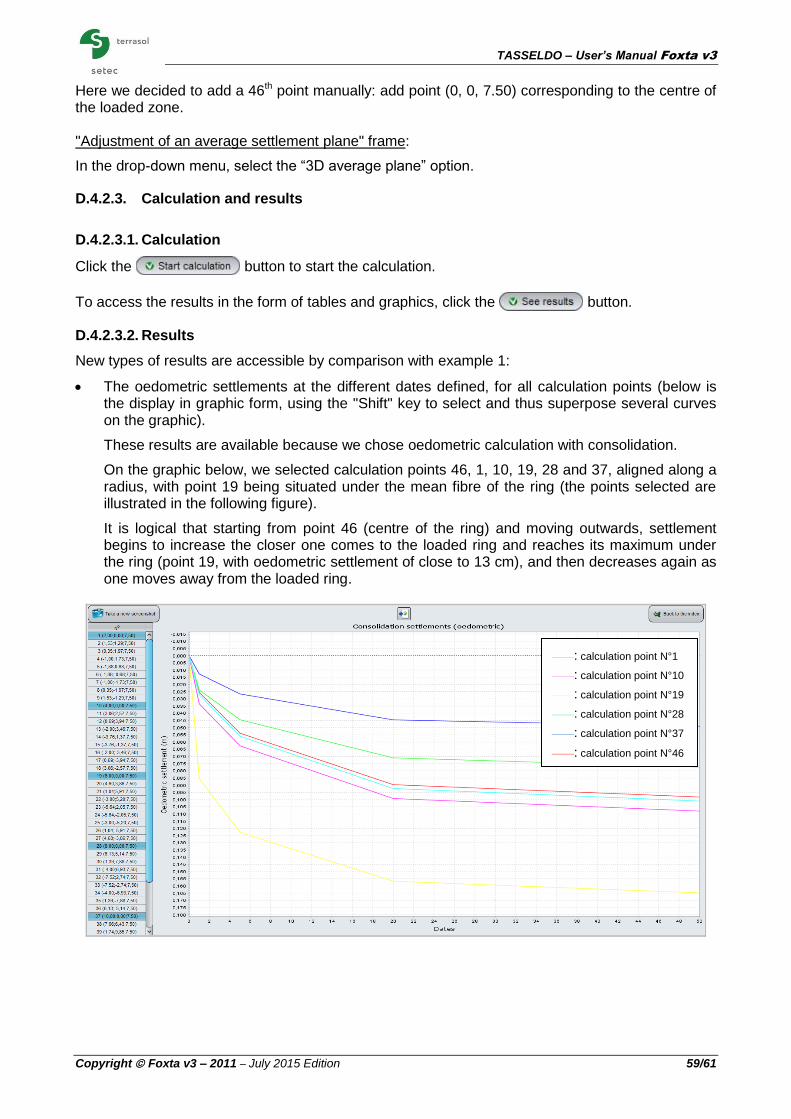
The oedometric settlements at the different dates defined, for all calculation points (below is the display in graphic form, using the "Shift" key to select and thus superpose several curves on the graphic).
These results are available because we chose oedometric calculation with consolidation.
On the graphic below, we selected calculation points 46, 1, 10, 19, 28 and 37, aligned along a radius, with point 19 being situated under the mean fibre of the ring (the points selected are illustrated in the following figure).
It is logical that starting from point 46 (centre of the ring) and moving outwards, settlement begins to increase the closer one comes to the loaded ring and reaches its maximum under the ring (point 19, with oedometric settlement of close to 13 cm), and then decreases again as one moves away from the loaded ring.
___: calculation point N°1
___: calculation point N°10
___: calculation point N°19
___: calculation point N°28
___: calculation point N°37
___: calculation point N°46

TASSELDO – User’s Manual Foxta v3
60/61 July 2015 Edition - Copyright Foxta v3 - 2011
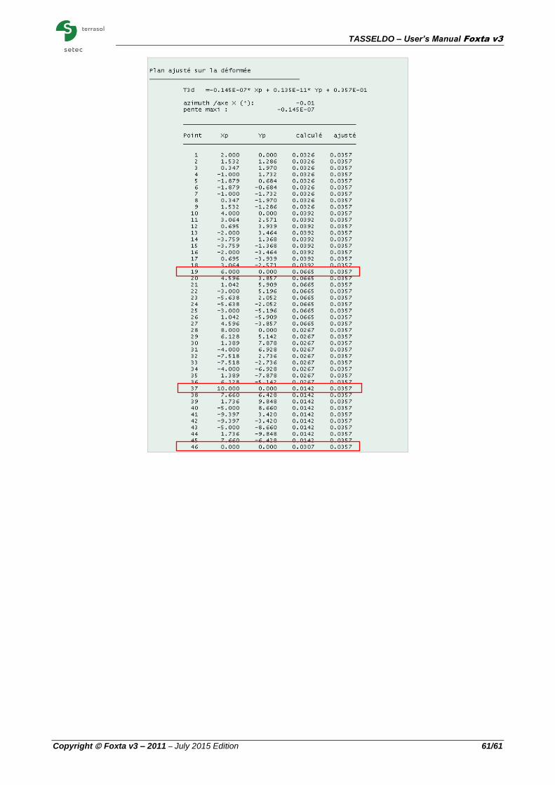
The 3D average plane equation, calculated on the basis of the 3D settlement of all the calculation points defined (average plane displayed below after the formatted numerical results).
It should be noted that the adjusted settlement (3D average plane for this example) is the same for all the calculation points: this corresponds to the uniform load case and a homogeneous distribution of calculation points under the loaded zone. The average plane settlement is here equal to 3.6 cm.
With regard to 3D elastic settlement, the “calculated” column tells us that it is maximal for the points situated below the loaded ring, as previously seen, with a value of 6.65 cm (point 19 for example). In addition and as expected, we see that settlement has the same value for all points situated on a given circle centred on the centre of the loaded ring, given that this is a uniform annular load.
46 37 28 19 10 1
TASSELDO – User’s Manual Foxta v3
Copyright Foxta v3 – 2011 – July 2015 Edition 61/61