Part 2: Wave Optics summary Wave motion (1)gwenlan/teaching/Optics-WO-HT18-4.pdf · CP2: Optics...
31
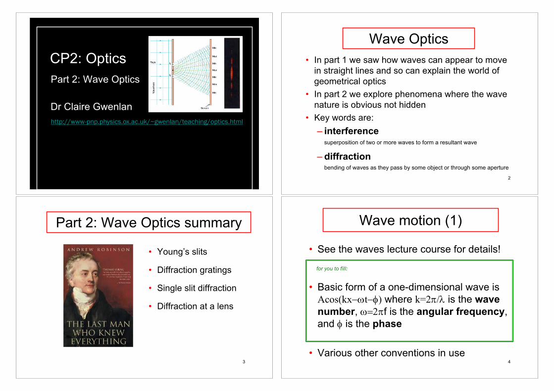
CP2: Optics Part 2: Wave Optics Dr Claire Gwenlan http://www-pnp.physics.ox.ac.uk/~gwenlan/teaching/optics.html Wave Optics • In part 1 we saw how waves can appear to move in straight lines and so can explain the world of geometrical optics • In part 2 we explore phenomena where the wave nature is obvious not hidden • Key words are: – interference superposition of two or more waves to form a resultant wave – diffraction bending of waves as they pass by some object or through some aperture 2 • Young’s slits • Diffraction gratings • Single slit diffraction • Diffraction at a lens 3 Part 2: Wave Optics summary Wave motion (1) • See the waves lecture course for details! • Basic form of a one-dimensional wave is Acos(kx-wt-f) where k=2p/l is the wave number, w=2pf is the angular frequency, and f is the phase • Various other conventions in use 4 for you to fill:
Transcript of Part 2: Wave Optics summary Wave motion (1)gwenlan/teaching/Optics-WO-HT18-4.pdf · CP2: Optics...
CP2: OpticsPart 2: Wave Optics
Dr Claire Gwenlanhttp://www-pnp.physics.ox.ac.uk/~gwenlan/teaching/optics.html
Wave Optics• In part 1 we saw how waves can appear to move
in straight lines and so can explain the world of geometrical optics
• In part 2 we explore phenomena where the wave nature is obvious not hidden
• Key words are:– interference
superposition of two or more waves to form a resultant wave
– diffractionbending of waves as they pass by some object or through some aperture
2
• Young’s slits
• Diffraction gratings
• Single slit diffraction
• Diffraction at a lens
3
Part 2: Wave Optics summary Wave motion (1)
• See the waves lecture course for details!
• Basic form of a one-dimensional wave is Acos(kx-wt-f) where k=2p/l is the wave number, w=2pf is the angular frequency, and f is the phase
• Various other conventions in use4
for you to fill:
Claire Gwenlan

• Basic wave is cos(kx-wt-f)• At time t the wave will look identical to its
appearance at time 0 except that it will have moved forward by a distance x=wt/k
• Wave moving the other way is described by cos(-kx-wt-f)
5
Wave motion (2)
• This is the basic equation for a wave on a string, but we can also use the same approach to describe a light wave travelling along the x-axis– More complex versions for general motion
• Oscillations in the electric and magnetic fields which vary in space and time just like the motion of a string
6
Plane wave (1)
Plane wave is a series of parallel wavefronts moving in one direction. Note that waves are really 3D: this is a 2D slice!
Mark the peaks of the waves as wavefronts
Draw normals to the wavefronts as rays7
Plane wave (2)
A plane wave impinging on a infinitesimal hole in a plate.
Acts as a point source and produces a spherical wave which spreads out in all directions.
Finite sized holes will be treated later.
8
Spherical wave

A plane wave impinging on a infinitesimal slit in a plate.
Acts as a point source and produces a cylindrical wave which spreads out in all directions.
Finite sized slits will be treated later.
Remainder of this course will use slits unless specifically stated
9
Cylindrical wave Obliquity Factor
• A more detailed treatment due to Fresnel shows that a point source does not really produce a spherical wave. Instead there is more light going forwards than sideways– Described by the obliquity factor
K=½(1+cosq)– Also explains lack of backwards wave– Not really important for small angles – Ignored in what follows
10
A plane wave impinging on a pair of slits in a plate will produce two circular waves
Where these overlap the waves will interfere with one another, either reinforcing or cancelling one another
Intensity observed goes as square of the total amplitude
11
Two slits
Constructive: intensity=4
+
=
Destructive: intensity=0
+
=
12
Sources should be monochromatic and coherent
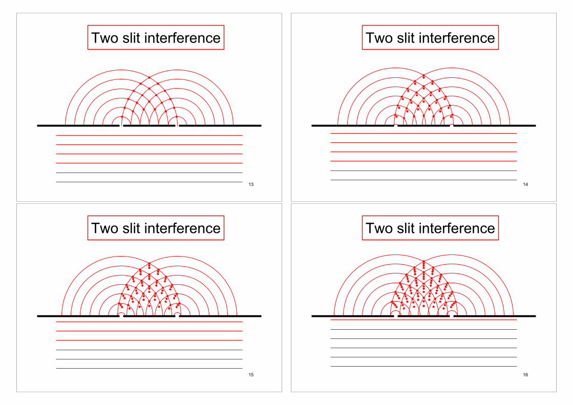
Interference
13
Two slit interference
14
Two slit interference
15
Two slit interference
16
Two slit interference
17
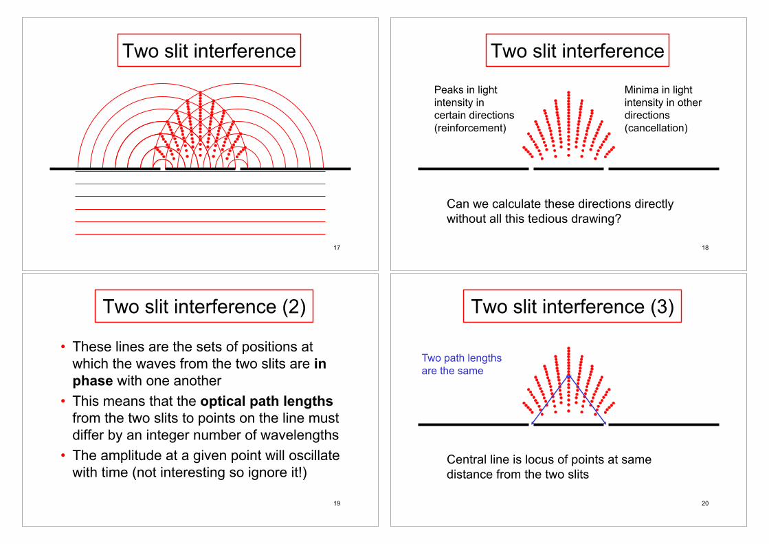
Two slit interference
Peaks in light intensity in certain directions (reinforcement)
Minima in light intensity in other directions (cancellation)
Can we calculate these directions directly without all this tedious drawing?
18
Two slit interference
• These lines are the sets of positions at which the waves from the two slits are in phase with one another
• This means that the optical path lengths from the two slits to points on the line must differ by an integer number of wavelengths
• The amplitude at a given point will oscillate with time (not interesting so ignore it!)
19
Two slit interference (2)
Central line is locus of points at same distance from the two slits
Two path lengths are the same
20
Two slit interference (3)

Next line is locus of points where distance from the two slits differs by one wavelength
Path lengths related by xleft=xright+l
xleft xright
21
Two slit interference (4)
Next line is locus of points where distance from the two slits differs by one wavelength
Path lengths related by xleft=xright+l
xleft xright
d
22
Two slit interference (5)
d
D
Interference pattern observed on a distant screen
yq
As d,y<<D the three blue lines are effectively parallel and all make an angle q»tanq=y/D to the normal. The bottom line is slightly longer than the top.
23
Two slit interference (6)
screen
Green line is normal to the blue lines, and forms a right angled triangle with smallest angle q. Its shortest side is the extra path length, and is of size δ=d×sin(q) » dy/D
24
Two slit interference (7)
d q
Close up
δδ=d×sin(q) » dy/D
for you to fill:

Two slit interference (8)
EG. taking l=500nm, d=1mm, D=1m, gives a fringe separation of 0.5mm 25
View at the screen
lD/d
Central fringe midway between slits
Maximum order: n < d/lDark fringes seen when y=(n+½)lD/d
Bright fringes seen when the extra path length is an integer number of wavelengths, so y=nlD/d
for you to fill:d
Alternative derivation
26
Two slit interference (9)
for you to fill:x1
x2
D
y δ = x2 − x1
x1 = (D2 + (y− d
2)2 )1/2
x2 = (D2 + (y+ d
2)2 )1/2
δ = x2 − x1 = D(1+(y+ d / 2)2
D2 )1/2 −D(1+ (y− d / 2)2
D2 )1/2
=12D
(y2 + d 2 / 4+ yd)− 12D
(y2 + d 2 / 4− yd) =ydD
Lloyd’s Mirror
• There are a very large number of similar two-source interference experiments
• Lloyd’s Mirror features on the practical course!
• Uses the interference between light from a slit and its virtual image in a plane mirror– See also Fresnel’s mirror, Fresnel’s biprism
27
Figure from script for OP0128
Lloyd’s Mirror

• Young’s slits form an interference pattern on a screen at any distance– Not an image!– At large distances the interference points lie
on straight lines at constant angles• Increasing the distance to the screen
increases the separation between the fringes but decreases their brightness
29
Practicalities: the screen
• The treatment above assumes that the slits act as point sources– Means that fringes can’t be very bright
• As slits get broader the outer fringes become less intense– We will come back to this once we have
looked at single slit diffraction– Not a problem as long as slit width is much
smaller than slit separation– Allows central fringe to be identified!
30
Practicalities: the slits
• Young’s slits assumes a light source providing uniform plane wave illumination
• Simplest approach is to assume a point source far from the slits– Spherical waves look like plane waves at a long
distance from the source• Such sources are not very bright
31
Practicalities: the source (1)
• A plane wave corresponds to a set of parallel rays
• This can be achieved by placing a point source at the focus point of a converging lens
• Can do a similar trick to see the fringes more clearly (more of this when we look at gratings)
32
Practicalities: the source (2)
• Still necessary to use a point source to avoid interference between light coming from different parts of the source!
• Detailed calculation is similar to that for slit size, so the source only needs to be small rather than a true point.
• Also turns out you can use a source slit as long as it is parallel to the two slits
33
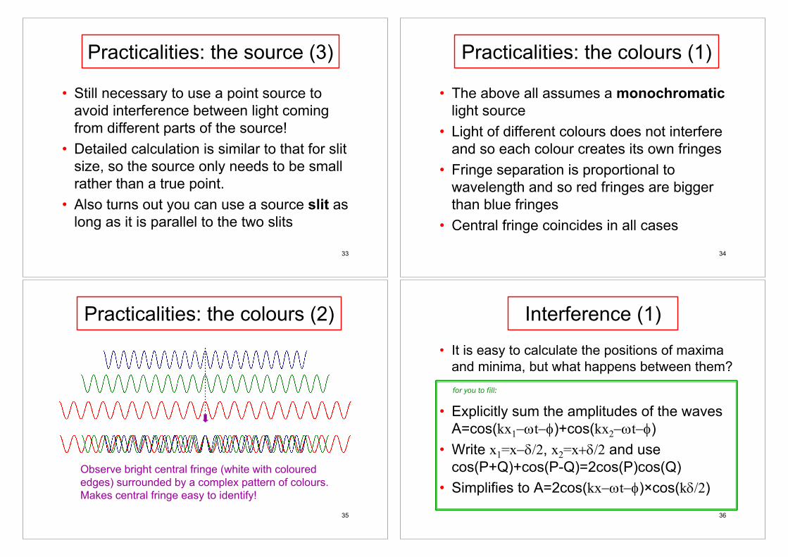
Practicalities: the source (3)
• The above all assumes a monochromaticlight source
• Light of different colours does not interfere and so each colour creates its own fringes
• Fringe separation is proportional to wavelength and so red fringes are bigger than blue fringes
• Central fringe coincides in all cases
34
Practicalities: the colours (1)
Observe bright central fringe (white with coloured edges) surrounded by a complex pattern of colours. Makes central fringe easy to identify!
35
Practicalities: the colours (2)
• It is easy to calculate the positions of maxima and minima, but what happens between them?
• Explicitly sum the amplitudes of the waves A=cos(kx1-wt-f)+cos(kx2-wt-f)
• Write x1=x-d/2, x2=x+d/2 and use cos(P+Q)+cos(P-Q)=2cos(P)cos(Q)
• Simplifies to A=2cos(kx-wt-f)×cos(kd/2)
36
Interference (1)
for you to fill:

• Amplitude is A=2cos(kx-wt-f)×cos(kd/2)• Intensity goes as square of amplitude so
I=4cos2(kx-wt-f)×cos2(kd/2)• First term is a rapid oscillation at the
frequency of the light (can replace by its average of ½); all the interest is in the second term
• I=2cos2(kd/2)=2[1+cos(kd)]/237
Interference (2)
for you to fill: • Intensity is: I=I0cos2(kd/2)= ½I0(1+cos(kd))
• Intensity oscillates with maxima at kd=2npand minima at kd=(2n+1)p
• Path length difference is d=dy/D• Maxima at y=Dd/d with d=2np/k and k=2p/l
giving y=nlD/d
38
Interference (3)
• Whenever you see a cosine you should consider converting it to an exponential! exp(ix)=cos(x)+ i sin(x)
• Basic wave in exponential form is cos(kx-wt-f)=Re{exp[i(kx-wt-f)]}
• Do the calculations in exponential form and convert back to trig functions at the very end
39
Exponential waves (1)• Repeat the interference calculation• Explicitly sum the amplitudes of the waves
• A=Re{exp[i(kx-kd/2-wt-f)]+exp[i(kx+kd/2-wt-f)]} =Re{exp[i(kx-wt-f)]×(exp[-ikd/2]+exp[+ikd/2])} =Re{exp[i(kx-wt-f)]×2cos[kd/2]} =2cos(kx-wt-f)×cos[kd/2]}
Same result as before (of course!) but can be a bit simpler to calculate
Will use complex waves where convenient from now on 40
Exponential waves (2)
for you to fill:
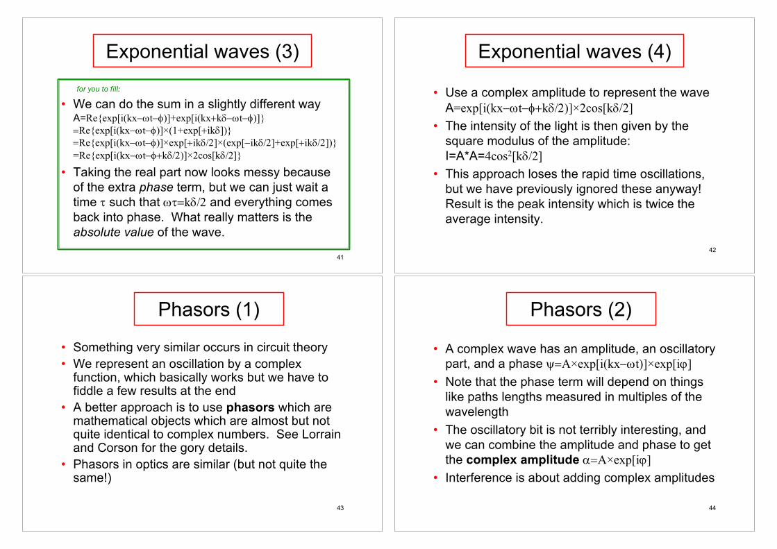
• We can do the sum in a slightly different wayA=Re{exp[i(kx-wt-f)]+exp[i(kx+kd-wt-f)]} =Re{exp[i(kx-wt-f)]×(1+exp[+ikd])} =Re{exp[i(kx-wt-f)]×exp[+ikd/2]×(exp[-ikd/2]+exp[+ikd/2])} =Re{exp[i(kx-wt-f+kd/2)]×2cos[kd/2]}
• Taking the real part now looks messy because of the extra phase term, but we can just wait a time t such that wt=kd/2 and everything comes back into phase. What really matters is the absolute value of the wave.
41
Exponential waves (3)
for you to fill: • Use a complex amplitude to represent the waveA=exp[i(kx-wt-f+kd/2)]×2cos[kd/2]
• The intensity of the light is then given by the square modulus of the amplitude: I=A*A=4cos2[kd/2]
• This approach loses the rapid time oscillations, but we have previously ignored these anyway! Result is the peak intensity which is twice the average intensity.
42
Exponential waves (4)
• Something very similar occurs in circuit theory• We represent an oscillation by a complex
function, which basically works but we have to fiddle a few results at the end
• A better approach is to use phasors which are mathematical objects which are almost but not quite identical to complex numbers. See Lorrain and Corson for the gory details.
• Phasors in optics are similar (but not quite the same!)
43
Phasors (1)
• A complex wave has an amplitude, an oscillatory part, and a phase y=A×exp[i(kx-wt)]×exp[ij]
• Note that the phase term will depend on things like paths lengths measured in multiples of the wavelength
• The oscillatory bit is not terribly interesting, and we can combine the amplitude and phase to get the complex amplitude a=A×exp[ij]
• Interference is about adding complex amplitudes
44
Phasors (2)

• We can represent a complex amplitude as a two dimensional vector on an Argand diagram
• We can then get the sum of complex amplitudes by taking the vector sum
Increasingly out of phase
Length of resultant is reduced Phase of resultant can mostly be ignored45
Phasors (3)example: two slit with phasors
46
Phasors (4)
for you to fill:
u0
u0up
φφ/2
up2 = (u0 + u0cosφ)2 + (u0sinφ)2
up2 = u0
2 + u02 + 2 u0
2cosφ
up2 = 2 u0
2(1+cosφ)
up2 = 4 u0
2 cos2φ
I = |up|2 = 4 u02 cos2φ
• In some cases elegant geometrical methods can be used to say something about the sum of a set of phasors without doing tedious calculations
• No calculations actually require phasors to be used, and at this level they are not terribly useful
• Don’t worry about them too much!
47
Phasors (5)
• Optical Path Length (n × geometric distance)is the distance that light would travel in air, in the same time as it took to travel a geometric distance w through a medium of refractive index n
• In medium of refractive index n, time taken for light to travel a distance w is: t = w/v = w/(c/n) = wn/c
• In air, in this same time, light would travel a distance = ct = wn (this is the Optical Path Length)
48
Optical path lengths (1)
for you to fill:

49
Optical path lengths (2)
• We can change the appearance of a two slit interference pattern by changing the optical path length for light from one of the two slits (OPL = n × geometric path length)
• Place a piece of transparent material with refractive index n and thickness w in front of one of the slits
• This increases the optical path length for light travelling through that slit by (n–1)×w, changing the phase of the light
• We could recalculate everything from first principles, but it is simplest just to note that the central fringe corresponds to the point where the optical path lengths for the two sources are identical
• Light travelling through the transparent material has travelled a longer optical path and so the central fringe must move towards this slit to ccompensate
50
Optical path lengths (3)
lD/d
Simple case: waves arrive at the slits in phase and the central interference peak is exactly between the slits
Fringes separated by lD/d 51
Optical path lengths (4)
One slit covered: waves arrive at the upper slit delayed by a wavelength and the central interference peak is moved up by a peak
52
central peak ⇾shifted to here
lD/d
Optical path lengths (5)

• Taking l=500nm, a piece of glass 0.1mm thick with n=1.5 gives a shift of 100 fringes
• The above all assumes that we can recognisethe central peak, but in the naïve treatment all peaks look the same!
• For white light fringes the central peak is easily recognised as the only clear white fringe
• For monochromatic light imperfections (notably the finite slit width) means that the central peak will be the brightest
53
Recognising the central peak
• It might seem odd that we always talk about the transparent material being placed before the slit rather than after it
• This means that we have to do the optical path calculations from some apparently arbitrary point before the slit
• Why not place the transparent material after the slit?
54
Optical path lengths (6)
Situation superficially similar to the previous case, but in fact the light will travel through the transparent medium at an angle making calculations look messy!
?
55
Optical path lengths (7)
• What about the apparently arbitrary start point?• Rigorous approach is to start all calculations
from the source, not from near the slits• Also allows calculations on the effect of moving
the source nearer to one of the two slits!• This is also how you should think about
imperfections like finite source sizes: different parts of the source lie at different distances from the two slits.
56
Optical path lengths (8)

• A diffraction grating is an extension of a double slit experiment to a very large number of slits
• Gratings can work in transmission or reflection but we will only consider transmission gratings
• The basic properties are easily understood from simple sketches, and most of the advanced properties are (in principle!) off-syllabus
57
Diffraction gratings (1)
Circular waves are formed from each source
58
Diffraction gratings (2)
Huygens style reinforcement creates a forward wave
59
Diffraction gratings (3)
Also get reinforcement at angles!
60
Diffraction gratings (4)

Reinforcement comes from successive waves from neighbouring sources
61
Diffraction gratings (5)
Draw rays normal to the wavefronts
62
Diffraction gratings (6)
Points on a wavefront must be in phase, so the extra distances travelled must be multiples of a wavelength
l2l3l
4l5l
6l
63
Diffraction gratings (7)
From trigonometry we see that sin(q)=6l/6d where q is the angle between the ray direction and the normal
q
6l
6d
Basic diffraction equation: l=d sin(q) (1st order maximum)
q
64
Diffraction gratings (8)
for you to fill:

Can also get diffraction in the same direction if the wavelength is halved!
2l4l6l
8l10l
12l
General diffraction equation: nl=d sin(q)
q
65
Diffraction gratings (9)
• nl=d sin(q)• Different colours have
different wavelengths and so diffract at different angles
• Take red (l=650nm), green (l=550nm), and blue (l=450nm) light and d=1.5µm
n=0n=1
n=2
66
Dispersion (1)
• Angular Dispersion of a grating is: D=dq/dln=0
n=1
n=2
67
Dispersion (2)
• From: nl = d sin(q) dq/dl = n/d cos(q)
= n/√(d2-n2l2)• Increases with order
of the spectrum and when d»nl
• Note that high order spectra can overlap!
for you to fill: qLight from a source is passed through a narrow source, collimated with a lens, dispersed with a grating, focused with a lens, and then detected
Measure intensity as a function of q to get the spectrum (in practice it is better to measure 2q, the angle between lines). Real designs more complex!
68
Grating spectrometer
proper illumination of grating

• Gratings have many advantages– Dispersion can be calculated!– High orders lead to high resolution– Reflection gratings don’t need transparency
• Gratings have a few disadvantages– Intensity shared between different orders– Can be improved by blazing the grating
69
Prism or grating?
Wings of butterflies (Blue Morpho)
Opals
Compact discs
70
“Natural” diffraction gratings
We also need to work out what happens in other directions. Between n=0 and n=1 there is a direction where the light from adjacent sources exactly cancel each other out – just as for two slits!
l/23l/25l/2 2l3l l
71
Between the peaks (1)
Closer to n=0 there is a direction where light from groups of three adjacent sources exactly cancels out
With an infinite number of sources will get cancellation in every direction except for the main peaks!
l2l
phasors
72
Between the peaks (2)

1st minimum at:
With a finite number of sources the last effective cancellation will occur when the path length difference between the first and last sources is about l
phasors
»l
73
Between the peaks (3)
Nφ = 2π ⇒ φ=2π/N ⇒ kdsin(θ)= 2π/N dsin(θ)=λ/Nfor you to fill:
Resolution of a grating
• The angular resolution of a diffraction grating can be calculated from the above. If the grating has N slits then need l»Nd sinq»Ndq which gives an angular resolution of dq»l/Nd»l/W where W is the width of the grating
• Similar results can be calculated in many different ways, most of which are rather complicated but one of which we will see later…
74
• In the above we mostly treated diffraction gratings as a generalisation of a double slit. In general we sum the amplitudes of light waves coming from all sources, and the intensity is the square modulus of the total amplitude
• For continuous objects replace the sum by an integral. Best to use complex wave notation to make integrals simple
75
Fraunhofer diffraction (1)
• In the general case we have to use the full theory of Fresnel diffraction (nasty!)
• In many important cases can use the simpler Fraunhofer approach
• This applies when the phase of the light amplitude varies linearly across the object
• Ultimately leads to the use of Fourier transforms in optics (next year!)
76
Fraunhofer diffraction (2)
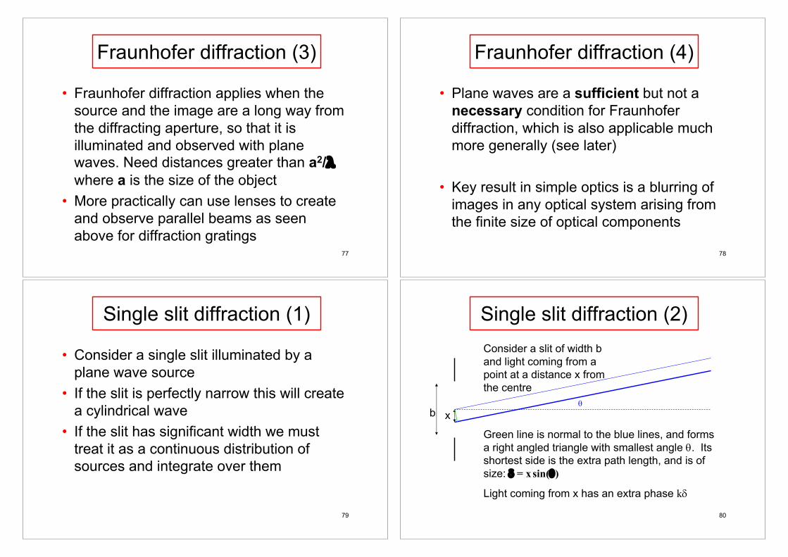
• Fraunhofer diffraction applies when the source and the image are a long way from the diffracting aperture, so that it is illuminated and observed with plane waves. Need distances greater than a2/!where a is the size of the object
• More practically can use lenses to create and observe parallel beams as seen above for diffraction gratings
77
Fraunhofer diffraction (3)
• Plane waves are a sufficient but not a necessary condition for Fraunhoferdiffraction, which is also applicable much more generally (see later)
• Key result in simple optics is a blurring of images in any optical system arising from the finite size of optical components
78
Fraunhofer diffraction (4)
• Consider a single slit illuminated by a plane wave source
• If the slit is perfectly narrow this will create a cylindrical wave
• If the slit has significant width we must treat it as a continuous distribution of sources and integrate over them
79
Single slit diffraction (1)
bq
Green line is normal to the blue lines, and forms a right angled triangle with smallest angle q. Its shortest side is the extra path length, and is of size: d = xsin(q)
x
Consider a slit of width b and light coming from a point at a distance x from the centre
Light coming from x has an extra phase kd
80
Single slit diffraction (2)

• Final amplitude is obtained by integrating over all points x in the slit and combining the phases, most simply in complex form
• A = ∫exp(ikd) dx = ∫exp(ikxsin(q)) dx
• Integral runs from x=-b/2 to x=b/2 and then normalise by dividing by b
81
Single slit diffraction (3)
82
Single slit diffraction (4)
for you to fill:
A = (1/b) ∫-b/2 b/2 exp(ik x sin(q)) dx
= 1/[ikbsin(q)] [exp(i(kb/2)sin(q)) – exp(-i(kb/2) sin(q))]
= 2i/[iksin(q)b] sin[(kb/2)sin(q)]
= sin[(kb/2)sin(q)] / [(kb/2) sin(q)]
1/b factor is amplitude of each infinitesimal point source i.e. it equals (u0/b) with u0 being amplitude from whole slit, and which is normalised to 1 here, as “usual”
• A = sin[(kb/2)sin(q)]/[(kb/2)sin(q)]• A = sin(b)/b with b= (kb/2)sin(q)
• Light intensity goes as the square of A• I=I0[sin(b)/b]2
• I= I0sinc2(b)
83
Single slit diffraction (5)
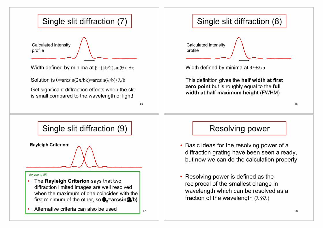
Calculated intensity profile
Maximum at b=0
Minimum at b=±pSubsidiary maximum near b=±3p/2
Width defined by minima at b=(kb/2)sin(q)=±p84
Single slit diffraction (6)
Calculated intensity profile
Width defined by minima at b=(kb/2)sin(q)=±p
Solution is q=arcsin(2p/bk)=arcsin(l/b)»l/b
Get significant diffraction effects when the slit is small compared to the wavelength of light!
85
Single slit diffraction (7)
Calculated intensity profile
Width defined by minima at q≈±l/b
This definition gives the half width at first zero point but is roughly equal to the full width at half maximum height (FWHM)
86
Single slit diffraction (8)
• The Rayleigh Criterion says that two diffraction limited images are well resolved when the maximum of one coincides with the first minimum of the other, so !R=arcsin("/b)
• Alternative criteria can also be used 87
Single slit diffraction (9)
Rayleigh Criterion:
for you to fill:
• Basic ideas for the resolving power of a diffraction grating have been seen already, but now we can do the calculation properly
• Resolving power is defined as the reciprocal of the smallest change in wavelength which can be resolved as a fraction of the wavelength (l/dl)
88
Resolving power
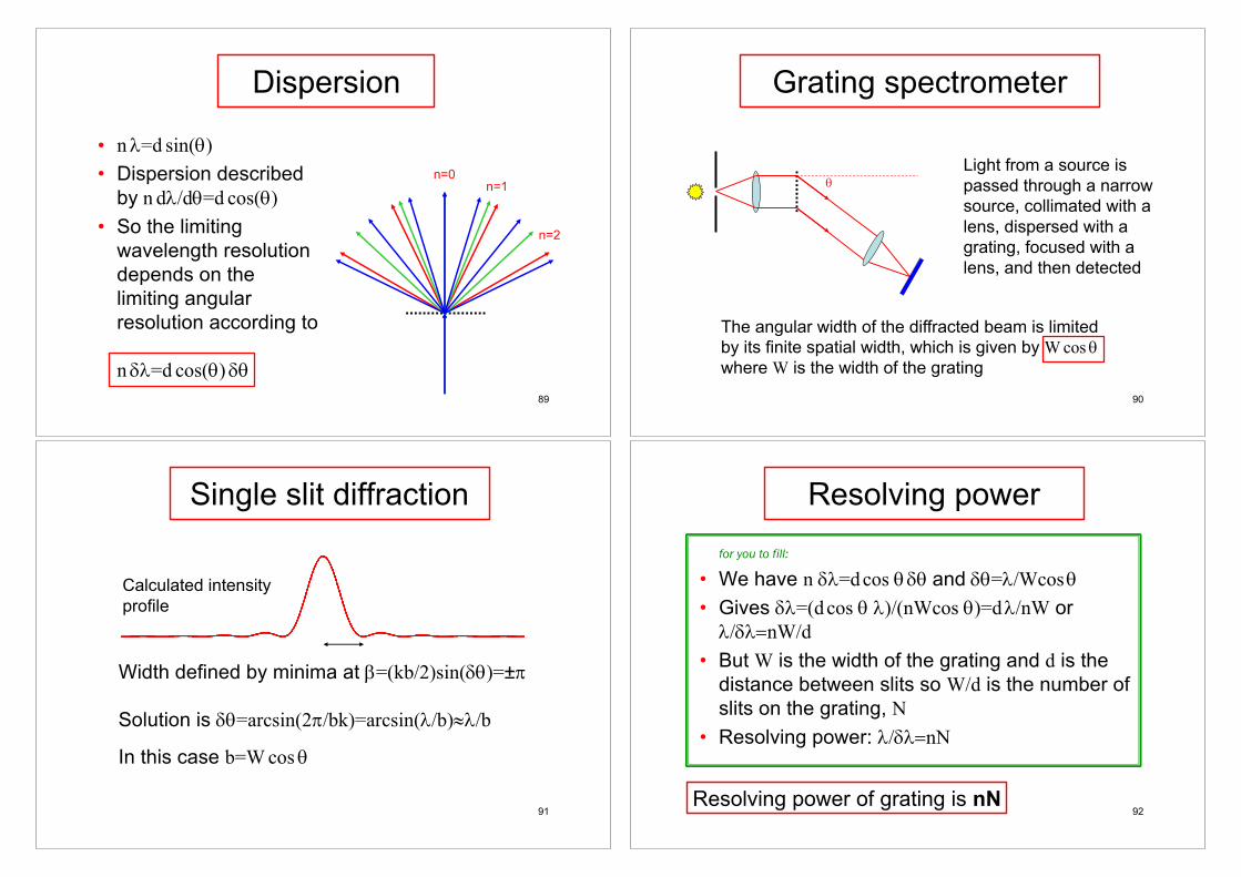
• nl=d sin(q)• Dispersion described
by n dl/dq=d cos(q)• So the limiting
wavelength resolution depends on the limiting angular resolution according to k n dl=d cos(q) dq
n=0n=1
n=2
89
Dispersion
qLight from a source is passed through a narrow source, collimated with a lens, dispersed with a grating, focused with a lens, and then detected
The angular width of the diffracted beam is limited by its finite spatial width, which is given by Wcos qwhere W is the width of the grating
90
Grating spectrometer
Calculated intensity profile
Width defined by minima at b=(kb/2)sin(dq)=±p
Solution is dq=arcsin(2p/bk)=arcsin(l/b)»l/b
In this case b=Wcos q
91
Single slit diffraction
• We have n dl=d cos qdq and dq=l/Wcosq• Gives dl=(d cos q l)/(nWcos q)=dl/nW or l/dl=nW/d
• But W is the width of the grating and d is the distance between slits so W/d is the number of slits on the grating, N
• Resolving power: l/dl=nN
92
Resolving powerfor you to fill:
Resolving power of grating is nN

Slit width (two slits)
• The traditional treatment of the double slit experiment is that each narrow slit acts as a source of circular waves that interfere
• If the slits have finite width b they will only produce intense waves within an angle q=arcsin(l/b)»l/b and only see around d/b fringes where d is the slit separation
• See problem set for better treatment
93
• A real slit is narrow in one dimension and very long (but not infinite!) in another
• The problem of a real slit can be solved in much the same way as an ideal slit but we now have to integrate over two dimensions
• Result is diffraction in both dimensions but the effect of the finite slit length can be neglected if it is many wavelengths long
94
Rectangular apertures
• The case of a circular hole is much like a square hole except that we have rotational symmetry
• Best solved by integrating in circular polar coordinates. This turns out to be a standard integral leading to a Bessel function
• Intensity is an Airy pattern with a bright Airy disk surrounded by Airy rings
• The resulting resolution is dq»1.22l/W (radius of the Airy disk)
95
Circular apertures
96
Airy disk and rings
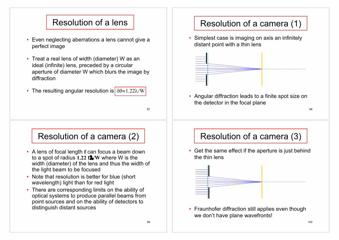
• Even neglecting aberrations a lens cannot give a perfect image
• Treat a real lens of width (diameter) W as an ideal (infinite) lens, preceded by a circular aperture of diameter W which blurs the image by diffraction
• The resulting angular resolution is dq»1.22l/W
97
Resolution of a lens• Simplest case is imaging on axis an infinitely
distant point with a thin lens
• Angular diffraction leads to a finite spot size on the detector in the focal plane
98
Resolution of a camera (1)
• A lens of focal length f can focus a beam down to a spot of radius 1.22 fl/W where W is the width (diameter) of the lens and thus the width of the light beam to be focused
• Note that resolution is better for blue (short wavelength) light than for red light
• There are corresponding limits on the ability of optical systems to produce parallel beams from point sources and on the ability of detectors to distinguish distant sources
99
Resolution of a camera (2)• Get the same effect if the aperture is just behind
the thin lens
• Fraunhofer diffraction still applies even though we don’t have plane wavefronts!
100
Resolution of a camera (3)

• Get the same effect even if the aperture is well behind the thin lens
• Aperture behind the lens has the same effect as a larger aperture at the lens (similar triangles)
101
Resolution of a camera (4)
• Imagine surrounding the aperture with diverging and converging thin lenses
• This has no overall effect on the rays but causes the aperture to be illuminated with plane waves, so get Fraunhofer diffraction
• Any aperture causes Fraunhofer diffraction when observed in the image plane!
102
Resolution of a camera (5)
Resolution of a telescope
• Resolution is usually limited by the width of the objective lens or the primary mirror
• Must ensure that all subsequent optical components are big enough that they don’t cut the beam down further
• Simple, as focussing of beams means that all later components will be smaller than the objective
103
• The pupil of the human eye gives a limiting angular resolution around 0.1mrad (20arcsec). This corresponds to resolving the headlights on a car about 20km away. With a small 125mm telescope the resolution is about 20 times better!
• Wavelength is just as important as diameter: the Arecibo telescope (300m diameter) has a limiting angular resolution of about 0.1mrad for 3cm radiation, but only 25mrad at 6m
104
Examples

• Simplest approach is to work backwards and find the smallest spot size to which a beam of light can be focused
• In the paraxial limit we already know that the limiting spot size is 1.22lf/W and the smallest resolvable feature has size 1.22lf/W
• General case was solved by Abbe using an analogy with diffraction gratings
105
Resolution of a microscope (1)
• Abbe showed that the smallest resolvable feature has size l/(2sin(a)) where a is half the angle subtended by the lens as seen from the focal plane
• For the paraxial case 2sin(a)≈ tan(2a)≈W/fin agreement with previous result
• As sin(a) cannot exceed 1 the limit on resolution by any lens is l/2
106
Resolution of a microscope (2)
• Can improve resolution still further by filling space between object and lens with fluid of refractive index n (oil objective)
• Limit is now l/(2 NA) where NA=nsin(a) is the Numerical Aperture of the lens
• Given typical refractive indices the limiting resolution of a microscope is about l/3≈135nm for blue light
107
Resolution of a microscope (3) Interference and Coherence
• Proper treatment of interference between different colours
• Coherence and its effects on interference
108

• The above all assumes a monochromatic light source
• Light of different colours does not interfere and so each colour creates its own fringes
• Fringe separation is proportional to wavelength and so red fringes are bigger than blue fringes
• Central fringe coincides in all cases
109
Practicalities: colours (1)
Observe bright central fringe (white with coloured edges) surrounded by a complex pattern of colours. Makes central fringe easy to identify!
110
Practicalities: colours (2)
• Does it really make sense to talk about interference only occurring between light of exactly the same colour? No source is truly monochromatic!
• Interference occurs by summation of amplitudes and surely this occurs whatever the waves look like?
111
Questions: colours
• Replace the two slits by two idealised sources of waves. If the two sources produce identical waves in phase with one another then the result will be identical to two slits!
• Perfectly practical with radio waves112
Two source interference

• If the two sources produce waves of different colours there will still be points where the amplitudes add constructively and destructively so will still get some sort of interference!
113
Two source interference
• Use complex amplitudes to represent the waves A=exp[i(kx-wt)]
• The intensity of the light is then given by half of the square modulus of the amplitude: I=½A*A
• This approach loses the rapid time oscillations, which occur at the frequency of the light. The factor of ½ is obtained by averaging over these. Rigorous calculations give the same result.
114
Exponential wave analysis (1)
• Consider interference between identical sources at distances x1=x-dx/2 and x2=x+dx/2
• A=exp[i(k(x-dx/2)-wt)]+exp[i(k(x+dx/2)-wt)]• A=exp[i(kx-wt)]×2cos[kdx/2]
• I=½A*A=2cos2[kdx/2]=1+cos[kdx]
• Standard interference pattern calculated before115
Exponential wave analysis (2)
• Now consider two different sources
• A=exp[i(k1(x-dx/2)-w1t)]+exp[i(k2(x+dx/2)-w2t)]
• I=½A*A=1+cos[½ (k1+k2)dx-(k1-k2)x+(w1-w2)t]
• k1=k-dk/2, k2=k+dk/2, w1=w-dw/2, w2=w+dw/2
• I=1+cos[k dx+dk x-dw t]
116
Exponential wave analysis (3)
for you to fill:

• I=1+cos[k dx-dk x+dw t]
• The third term indicates that the interference pattern looks like a travelling wave and moves across the screen. The light intensity at any point oscillates at frequency dw
• If the detector (camera, eye, etc.) has a response time slow compared with 1/dw then the pattern will wash out to the average intensity of 1
117
Exponential wave analysis (4)
• Thus we will only see interference patterns from two sources if their frequencies are closely matched compared with the response time of the detector!
• Now need to consider what happens if there are sources emitting two frequencies at bothpositions. The analysis is messy but not too bad with help from an algebra program
118
Exponential wave analysis (5)
• Result is a time varying term, which averages to zero, and a constant term which must be kept
• I=2+2cos[k dx]cos[dk dx/2]
• This is exactly the same result as you get by adding together two separate intensity patterns
• I=1+cos[(k-½dk) dx]+1+cos[ (k+½dk) dx]119
Exponential wave analysis (6)
Patterns of constructive and destructive interference between two sets of fringes leads to a beat pattern in the total intensity
120
Two colours
• The normal two slits analysis derives two coherent sources by dividing the wavefrontsfrom a single source. We see interference between wavefronts which have left the source at different times.
• This only works if the time gap is small compared with the coherence time of the source which depends on the frequency bandwidth of the source: sharp frequency sources give more fringes!
121
Temporal coherence
• Spatial coherence describes the coherence between different wavefronts at different points in space. It is rather more complicated than temporal coherence as it also depends on the size (angular diameter) of the source
• Can be used the measure the angular diameter of the source! This is the basis of Michelson’s stellar interferometer
• See Introduction to Modern Optics by Grant R. Fowles
122
Spatial coherence