The workers and union movement in China June 3 rd, 2014 BCFL/VDLC Delegation.
Pareto weights as wedges in two-country models∗
David Backus,† Chase Coleman,‡ Axelle Ferriere,§ and Spencer Lyon¶
Revised: November 27, 2015
Abstract
In models with recursive preferences, endogenous variation in Pareto weights wouldbe interpreted as wedges from the perspective of a frictionless model with additivepreferences. We describe the behavior of the (relative) Pareto weight in a two-countryworld and explore its interaction with consumption and the real exchange rate.
JEL Classification Codes: F31, F41.
Keywords: recursive preferences; consumption and risk-sharing; real exchange rate.
∗Prepared for the Fed St. Louis-JEDC-SCG-SNB-UniBern Conference, Gerzensee, October 2015.We thank Jarda Borovicka, Riccardo Colacito, and John Stachurski for helpful advice. We also thankthe conference participants, including especially Giancarlo Corsetti, Robert Kollmann, Ayhan Kose,and Ravi Ravikumar. James Bullard suggested the analogy with wedges. We will post the codeshortly at https://github.com/NYUEcon/BCFL2016.† Stern School of Business, New York University, and NBER; [email protected].‡ Stern School of Business, New York University; [email protected].§ European University Institute; [email protected].¶ Stern School of Business, New York University; [email protected].

1 Introduction
We explore the effects of recursive preferences and risk in an otherwise standard two-
country exchange economy. We focus on the behavior of the (relative) Pareto weight,
which characterizes consumption allocations across countries. When preferences are
additive over time and across states, as they typically are, the Pareto weight is con-
stant in frictionless environments. But when preferences are recursive and agents
consume different goods, the Pareto weight can fluctuate even in frictionless environ-
ments. This variation in the Pareto weight acts like a wedge from the perspective of
an additive model. Among the potential byproducts are changes in the behavior of
consumption and the exchange rate.
The natural comparison is with models that use capital market frictions to resolve
some of the anomalous features of the standard model. Baxter and Crucini (1995),
Corsetti, Dedola, and Leduc (2008), Heathcote and Perri (2002), Kehoe and Perri
(2002), and Kose and Yi (2006) are well-known examples. The frictions in these pa-
pers might be viewed as devices to produce variation in the Pareto weight, which is
then reflected in prices and quantities. In the language of Chari, Kehoe, and McGrat-
tan (2007), variations in Pareto weights would look look like wedges in the frictionless
model. The question for both approaches is whether these wedges are similar to those
we observe when we confront frictionless models with evidence. Ultimately we would
like to understand how the two approaches compare, but for now we’re simply trying
to understand how the Pareto weight works in models with recursive preferences.
We build in an obvious way on earlier work with multi-good economies by Colacito
and Croce (2013, 2014), Colacito, Croce, Ho, and Howard (2014), Kollmann (2015),
and Tretvoll (2011, 2013, 2015). We show how their models work and introduce some
modest extensions. We also build on the fundamental work on recursive risk-sharing
by Anderson (2005), Borovicka (2015), and Collin-Dufresne, Johannes, and Lochstoer
(2015). These papers study one-good worlds, and in that respect are simpler than
work with multi-good international models, but they lay out the structure of re-
cursive risk-sharing problems. The last paper in the list also describes an effective
computational method which we adapt to our environment.

One byproduct is a clearer picture of what drives the dynamics of the Pareto weights.
In many one-good economies, Pareto weights aren’t stable. Eventually one agent
consumes everything. One of the insights of Colacito and Croce (2013) is that home
bias and imperfect substitutability between goods can produce stable processes for
Pareto weights and consumption shares. That’s true here, as well, but we also show
how changes in risk aversion and intertemporal substitutability affect the dynamics of
the Pareto weight. Relative to the additive case, increasing risk aversion or decreasing
intertemporal substitution generates more persistence in the real exchange rate. Since
real exchange rates are very persistent in the data, this novel source of persistence is
a welcome one.
Risk is a particularly interesting object in this context. Random changes in the
relative supply of foreign and domestic goods also affect demand — with recursive
preferences — through their impact on future utility. As in many dynamic models,
it’s not clear here how (if?) we might separate the concepts of supply and demand. A
change in the conditional variance of future endowments, however, works only though
the second channel; supplies (endowments) do not change. Risk affects allocations
through its impact on the Pareto weight without any direct impact on supply.
All of these results are based on global numerical solutions to the Pareto problem.
These solutions take much more computer time than the perturbation methods used
in most related work, but they come with greater assurance that the solution is
accurate even in states far from the mean of the distribution.
Notation and terminology. We use Latin letters for variables and Greek letters for
parameters. Variables without time subscripts are means of logs. We use the term
steady state to refer to the mean of the log of a variable. Thus steady state x refers
to the mean value of log xt.
2 A recursive two-country economy
We study an exchange version of the Backus, Kehoe, and Kydland (1994) two-country
business cycle model. Like their model, ours has two agents (one for each country),
two intermediate goods (“apples” and “bananas”), and two final goods (one for each
2

country). Unlike theirs, ours has (i) exogenous output of intermediate goods, (ii) a
unit root in productivity, (iii) recursive preferences, and (iv) stochastic volatility in
productivity growth in one country. The first is for convenience. The second allows
us to produce realistic asset prices. We focus on the last two, specifically their role
in the fluctuations in consumption and exchange rates.
Preferences. We use the recursive preferences developed by Epstein and Zin (1989),
Kreps and Porteus (1978), and Weil (1989). Utility from date t on in country j is
denoted Ujt. We define utility recursively with the time aggregator V :
Ujt = V [cjt, µt(Ujt+1)] = [(1− β)cρjt + βµt(Ujt+1)ρ]1/ρ, (1)
where cjt is consumption in country j and µt is a certainty equivalent function. The
parameters are 0 < β < 1 and ρ ≤ 1. We use the power utility certainty equivalent
function,
µt(Ujt+1) =[Et(U
αjt+1)
]1/α, (2)
where Et is the expectation conditional on the state at date t and α ≤ 1. Preferences
reduce to the traditional additive case when α = ρ.
Both V and µ are homogeneous of degree one (hd1). The two functions together have
the property that if consumption is constant at c from date t on, then Ujt = c.
In standard terminology, 1/(1−ρ) is the intertemporal elasticity of substitution (IES)
(between current consumption and the certainty equivalent of future utility) and 1−αis risk aversion (RA) (over future utility). The terminology is somewhat misleading,
because changes in ρ affect future utility, the thing over which we are risk averse. As
in other multi-good settings, there’s no clean separation between risk aversion and
substitutability.
Technology. Each country specializes in the production of its own intermediate good,
“apples” in country 1 and “bananas” in country 2. In the exchange case we study,
production in country j equals its exogenous productivity:
yjt = zjt. (3)
3
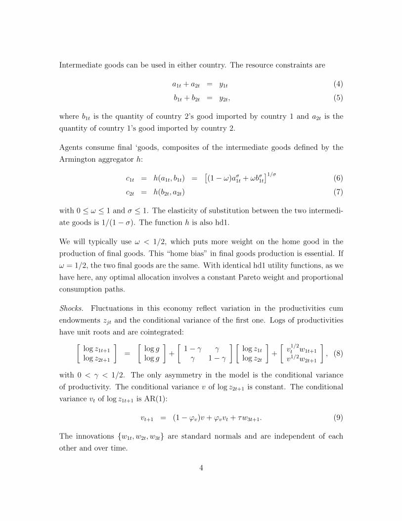
Intermediate goods can be used in either country. The resource constraints are
a1t + a2t = y1t (4)
b1t + b2t = y2t, (5)
where b1t is the quantity of country 2’s good imported by country 1 and a2t is the
quantity of country 1’s good imported by country 2.
Agents consume final ‘goods, composites of the intermediate goods defined by the
Armington aggregator h:
c1t = h(a1t, b1t) =[(1− ω)aσ1t + ωbσ1t
]1/σ(6)
c2t = h(b2t, a2t) (7)
with 0 ≤ ω ≤ 1 and σ ≤ 1. The elasticity of substitution between the two intermedi-
ate goods is 1/(1− σ). The function h is also hd1.
We will typically use ω < 1/2, which puts more weight on the home good in the
production of final goods. This “home bias” in final goods production is essential. If
ω = 1/2, the two final goods are the same. With identical hd1 utility functions, as we
have here, any optimal allocation involves a constant Pareto weight and proportional
consumption paths.
Shocks. Fluctuations in this economy reflect variation in the productivities cum
endowments zjt and the conditional variance of the first one. Logs of productivities
have unit roots and are cointegrated:[log z1t+1
log z2t+1
]=
[log glog g
]+
[1− γ γγ 1− γ
] [log z1tlog z2t
]+
[v1/2t w1t+1
v1/2w2t+1
], (8)
with 0 < γ < 1/2. The only asymmetry in the model is the conditional variance
of productivity. The conditional variance v of log z2t+1 is constant. The conditional
variance vt of log z1t+1 is AR(1):
vt+1 = (1− ϕv)v + ϕvvt + τw3t+1. (9)
The innovations {w1t, w2t, w3t} are standard normals and are independent of each
other and over time.
4

3 Features and parameter values
We describe some of the salient features of the model and the benchmark parameter
values we use later on.
Features
Consumption frontier. The resource constraints define a possibilities frontier for con-
sumption. We picture several examples in Figure 1, z1t = z2t = 1. In each case, we
compute the maximum quantity c1t consistent with a given quantity c2t, the resource
constraints (4,5), and the Armington aggregators (6,7). The shape depends on the
aggregator. When ω = 1/2, the two final goods are the same and the tradeoff is
linear. When ω 6= 1/2, the frontier is convex. The degree of convexity depends on
the elasticity of substitution 1/(1− σ) in the Armington aggregator.
In a competitive equilibrium, the slope of the consumption frontier is (minus) the
relative price of consumption in the two countries, p2t/p1t = et, the real exchange
rate. From the figure, we can imagine variation in this price produced either by
moving along the frontier or by changing the frontier through movements in the
quantities of intermediate goods.
Marginal rates of substitution. Competitive equilibria and Pareto optima equate
agents’ marginal rates of substitution (mrs for short). With recursive preferences, the
intertemporal mrs of agent j is
mjt+1 = β
(cjt+1
cjt
)ρ−1(Ujt+1
µt(Ujt+1)
)α−ρ. (10)
The last term summarizes the impact of recursive preferences. If α = ρ, preferences
are additive and the term disappears. Otherwise anything that affects future utility
can play a role in the marginal rate of substitution, hence in allocations. A change
in risk, for example, affects future utility, and through it consumption quantities
and prices. Persistence is critical here, because more persistent shocks have a larger
impact on future utility. The discount factor β is similar: the larger it is, the greater
the weight on future utility and the greater the impact on the mrs.
5

Note, too, the dynamics built into the recursive term. Its log is a risk adjustment
plus white noise. The log of the numerator is
logUjt+1 = Et(logUjt+1) +[
logUjt+1 − Et(logUjt+1)],
the mean plus a white noise innovation. The log of the denominator is
log µt(Ujt+1) = α−1 logEt(eα logUjt+1)
= Et(logUjt+1) + α−1[
logEt(eα logUjt+1)− Et(α logUjt+1)
].
The term in square brackets is the entropy of Uαjt+1 and is positive. We multiply by α
to get what we term the risk adjustment, which is negative if α is. The difference then
is the innovation minus the risk adjustment. The innovation increases the volatility
of the mrs, which is the primary source of success in asset pricing applications.
The mrs (10) is measured in units of agent j’s consumption good, whose price is pjt.
We refer to the relative price of the two consumption goods as the real exchange
rate: et = p2t/p1t. The two mrs’s are then connected by m2t+1 = (et+1/et)m1t+1.
We’ll derive this in the next section, but it should be evident here the dynamics of
the exchange rate reflect the mrs’s. If the two mrs’s are close to white noise, as we
suggested, then the depreciation rate et+1/et has the same property.
Productivity dynamics. One way to think about our log productivity process (8) is
that their average is a martingale and their difference is stable. Denote half the sum
and half the difference by
log z = (log z1 + log z2)/2
log z = (log z1 − log z2)/2.
Then we can express the underlying productivities by log z1 = log z + log z and
log z2 = log z − log z. Equation (8) implies that half the sum,
log zt+1 = log g + log zt + (v1/2t w1t+1 + v1/2w2t+1)/2,
is a martingale with drift. The difference,
log zt+1 = (1− 2γ) log zt + (v1/2t w1t+1 − v1/2w2t+1)/2, (11)
6

is stable, which tells us log z1t and log z2t are cointegrated. Given the linear homo-
geneity of the model, changes in z affect consumption quantities proportionately, with
no effect on their relative price, the exchange rate. Changes in relative productivity
z, however, affect consumption quantities differentially and therefore affect the real
exchange rate as well.
Pareto problems. We compute competitive equilibria in this environment by finding
Pareto optimal allocations and their supporting prices. In a two-agent Pareto prob-
lem, we maximize one agent’s utility subject to (i) the other agent getting at least
some promised level of utility (the promise-keeping constraint) and (ii) the productive
capacity of the economy (the resource constraints and shocks). The Lagrangian for
this problem is
L = U1t + λt(U2t − U) + resource constraints and shocks,
with λt the multiplier on the promise-keeping constraint. If utility functions are
strictly concave, this is equivalent to traditional Mantel-Negishi maximization of their
weighted average,
θ1tU1t + θ2tU2t,
with positive Pareto weights (θ1t, θ2t). Evidently λt in the previous problem plays the
same role as θ2t/θ1t. We refer to λt as the Pareto weight, although in terms of the
latter version we might call it the relative Pareto weight.
Transforming utility. We find it convenient to use an hd1 time aggregator, but with
additive preferences (the special case ρ = α) it’s more common to transform utility
to U∗jt = Uρjt/ρ. With this transformation, equation (1) becomes
U∗jt = (1− β)cρjt/ρ+ β[Et(U
∗α/ρjt+1 )
]ρ/α. (12)
When ρ = α this takes the familiar additive form.
The transformation also changes the look of derivatives. When we represent prefer-
ences with Ujt, marginal utility is
∂Ujt/∂cjt = U1−ρjt (1− β)cρ−1jt .
7

When we use U∗jt, marginal utility takes the simpler form
∂U∗jt/∂cjt = (1− β)cρ−1jt .
We’ll use this insight later on to simplify some of the expressions we get using the
hd1 form of the time aggregator. This includes the Pareto weight, which is defined
for a specific utility function.
Parameter values
We make only a modest effort to use realistic parameter values. The goal instead is to
highlight the effects of recursive preferences and stochastic volatility with parameter
values in the ballpark of those used elsewhere in the literature. We summarize these
choices in Table 1. The time interval is one quarter.
Preferences. We use ρ = −1 (implying an IES of one-half) and α = −9 (implying risk
aversion of 10). The former is a common value in business cycle modeling; Kydland
and Prescott (1982), for example. The latter is widely used in asset pricing; Bansal
and Yaron (2004) is the standard reference. The key feature of this configuration is
that α− ρ < 0. We set β = 0.98.
Technology. The Armington aggregator plays a central role here, specifically the
elasticity of substitution 1/(1−σ) between foreign and domestic intermediate goods.
A wide range of elasticities have been used in the literature. Some earlier work used
elasticities greater than one. Colacito and Croce (2013, 2014) and Kollman (2015)
use an elasticity of one. Heathcote and Perri (2002, Section 3.2) and Tretvoll (2013,
Table 1; 2015, Table 3) suggest smaller values. We start with an elasticity of one
(σ = 0), but consider other values, particularly when we explore the interaction of
the elasticity and the dynamics of the Pareto weight.
Given a choice of σ, we set the share parameter ω like this. First-order conditions
equate prices to marginal products:
p1t = c1−σ1t (1− ω)aσ−11t
p2t = c1−σ1t ωbσ−11t
8

In a symmetric steady state with import share sm = b1/(a1 + b1) and relative price
p2t/p1t = 1, the ratio of these two equations implies(1− ωω
)=
(1− smsm
)1−σ
. (13)
We set sm = 0.1. Given a value for σ, the import share nails down ω. One consequence
of this calculation is that the parameter ω approaches one-half as σ approaches one
(and the elasticity of substitution approaches infinity).
Shocks. The mean growth rate is log g = 0.004: 0.4% per quarter. The number comes
from Tallarini (2000, Table 4) and applies to the US. We set the persistence parameter
γ that governs productivity dynamics equal to 0.1, which implies an autocorrelation of
1− 2γ = 0.8 for log z. Rabanal, Rubio-Ramirez, and Tuesta (2011, Table 5) estimate
γ to be less than 0.01, which implies significantly greater persistence. The stochastic
volatility process (9) is based on Jurado, Ludvigson, and Ng (2014) as described in
Backus, Ferriere, and Zin (2014, Section 5.3).
4 Solving the recursive Pareto problem
We compute a competitive equilibrium indirectly as a Pareto optimum, a standard
approach in this literature. The competitive prices then show up as Lagrange multi-
pliers on the resource constraints. Similar models have been studied by Colacito and
Croce (2013), Kollman (2015), and Tretvoll (2011).
Pareto problem
We solve the Pareto problem recursively. We make a slight change in notation, and
represent utility of agent 1 by J , the value function, and the utility of agent 2 by
U , without the “2” subscript. The state at date t is then the exogenous variables
st = (z1t, z2t, vt) plus the utility promise Ut made to agent 2. The Bellman equation
is
J(Ut, st) = max{c1t,Ut+1}
V{c1t, µt[J(Ut+1, st+1)]
}s.t. V
{c2t, µt(Ut+1)
}≥ Ut
plus resource constraints and shocks.
9

The resource constraints include (4,5) for intermediate goods and (6,7) for final goods.
The shocks follow (8,9).
We use Lagrange multipliers λt on promised utility and (q1t, q2t, p1t, p2t) on the re-
source constraints. The first-order conditions are then
c1t : p1t = J1−ρt (1− β)cρ−11t (14)
c2t : p2t = λtU1−ρt (1− β)cρ−12t (15)
a1t : q1t = p1tc1−σ1t (1− ω)aσ−11t (16)
b1t : q2t = p1tc1−σ1t ωbσ−11t (17)
a2t : q1t = p2tc1−σ2t ωaσ−12t (18)
b2t : q2t = p2tc1−σ2t (1− ω)bσ−12t (19)
Ut+1 : J1−ρt βµt(Jt+1)
ρ−αJα−1t+1 JUt+1 = −λtU1−ρt βµt(Ut+1)
ρ−αUα−1t+1 . (20)
Note, in particular, that equation (20) applies to promises Ut+1 in every state at t+1.
It’s many equations, not just one.
The envelope condition for Ut is
JUt = −λt,
which we use to replace JUt+1 with λt+1 in (20).
Transforming the Pareto weight. We can simplify the solution by transforming the
Pareto weight λ. A Pareto weight is defined for specific a utility function; if we
transform the utility function, we transform the Pareto weight along with it. The
natural benchmark for the Pareto weight is the additive case, in which it’s constant.
Additive preferences are traditionally expressed using utility U∗t = Uρt /ρ and J∗t =
Jρt /ρ. The associated Pareto weight is
λ∗t = λtU1−ρt /J1−ρ
t .
We refer to λ∗t as the additive Pareto weight — or simply, when it’s clear, the Pareto
weight.
10
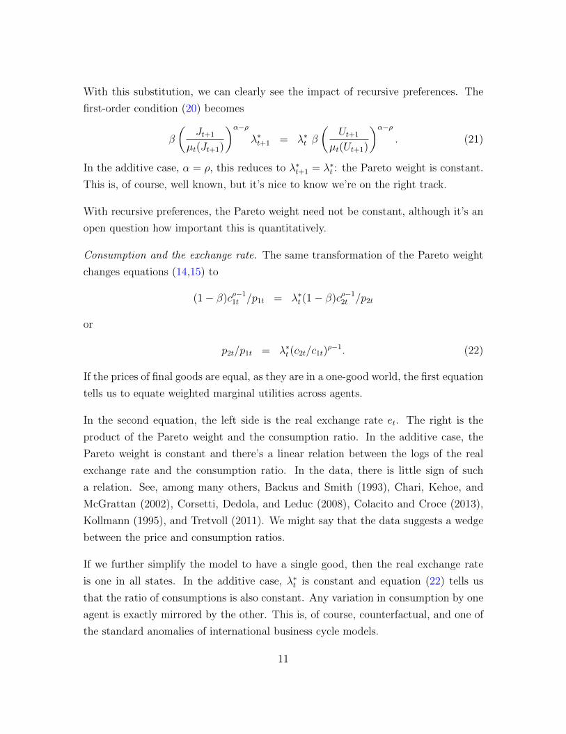
With this substitution, we can clearly see the impact of recursive preferences. The
first-order condition (20) becomes
β
(Jt+1
µt(Jt+1)
)α−ρλ∗t+1 = λ∗t β
(Ut+1
µt(Ut+1)
)α−ρ. (21)
In the additive case, α = ρ, this reduces to λ∗t+1 = λ∗t : the Pareto weight is constant.
This is, of course, well known, but it’s nice to know we’re on the right track.
With recursive preferences, the Pareto weight need not be constant, although it’s an
open question how important this is quantitatively.
Consumption and the exchange rate. The same transformation of the Pareto weight
changes equations (14,15) to
(1− β)cρ−11t /p1t = λ∗t (1− β)cρ−12t /p2t
or
p2t/p1t = λ∗t (c2t/c1t)ρ−1. (22)
If the prices of final goods are equal, as they are in a one-good world, the first equation
tells us to equate weighted marginal utilities across agents.
In the second equation, the left side is the real exchange rate et. The right is the
product of the Pareto weight and the consumption ratio. In the additive case, the
Pareto weight is constant and there’s a linear relation between the logs of the real
exchange rate and the consumption ratio. In the data, there is little sign of such
a relation. See, among many others, Backus and Smith (1993), Chari, Kehoe, and
McGrattan (2002), Corsetti, Dedola, and Leduc (2008), Colacito and Croce (2013),
Kollmann (1995), and Tretvoll (2011). We might say that the data suggests a wedge
between the price and consumption ratios.
If we further simplify the model to have a single good, then the real exchange rate
is one in all states. In the additive case, λ∗t is constant and equation (22) tells us
that the ratio of consumptions is also constant. Any variation in consumption by one
agent is exactly mirrored by the other. This is, of course, counterfactual, and one of
the standard anomalies of international business cycle models.
11
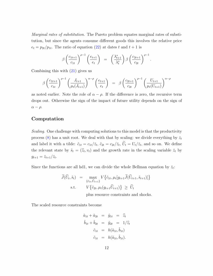
Marginal rates of substitution. The Pareto problem equates marginal rates of substi-
tution, but since the agents consume different goods this involves the relative price
et = p2t/p1t. The ratio of equation (22) at dates t and t+ 1 is
β
(c1t+1
c1t
)ρ−1(et+1
et
)=
(λ∗t+1
λ∗t
)β
(c2t+1
c2t
)ρ−1.
Combining this with (21) gives us
β
(c1t+1
c1t
)ρ−1(Jt+1
µt(Jt+1)
)α−ρ(et+1
et
)= β
(c2t+1
c2t
)ρ−1(Ut+1
µt(Ut+1)
)α−ρas noted earlier. Note the role of α − ρ. If the difference is zero, the recursive term
drops out. Otherwise the sign of the impact of future utility depends on the sign of
α− ρ.
Computation
Scaling. One challenge with computing solutions to this model is that the productivity
process (8) has a unit root. We deal with that by scaling: we divide everything by zt
and label it with a tilde: c1t = c1t/zt, c2t = c2t/zt, Ut = Ut/zt, and so on. We define
the relevant state by st = (zt, vt) and the growth rate in the scaling variable zt by
gt+1 = zt+1/zt.
Since the functions are all hd1, we can divide the whole Bellman equation by zt:
J(Ut, st) = max{c1t,Ut+1}
V{c1t, µt[gt+1J(Ut+1, st+1)]
}s.t. V
{c2t, µt(gt+1Ut+1)
}≥ Ut
plus resource constraints and shocks.
The scaled resource constraints become
a1t + a2t = y1t = zt
b1t + b2t = y2t = 1/zt
c1t = h(a1t, b1t)
c1t = h(a1t, b1t).
12

The laws of motion for the shocks are (11) for zt and (9) for vt (no scaling required).
zt drops out, leaving us with a lower-dimensional state.
Given a solution to the scaled problem, we can multiply by zt to produce a solution
to the original problem. The notation is horrendous. The point is simply that we can
convert our problem to one with stable shocks. And we do.
Algorithm. Another challenge in computing a solution is that at each date t, we
need to choose utility promises Ut+1 for every state the following period. We adapt
the algorithm of Collin-Dufresne, Johannes, and Lochstoer (2015) to a multi-good
setting. Their algorithm has three essential features. First, they make a clever choice
of state variable. Second, they use backward recursion, starting at a terminal date
and computing the value function recursively at earlier dates. Third, they use the
first-order conditions to solve for the optimal policies, rather than simply choosing
the best from a finite set of possibilities.
Consider the state variable. We characterized the problem using promised utility Ut
as the state. Collin-Dufresne, Johannes, and Lochstoer replace promised utility with
the consumption share. Given the consumption share, the conditions of the solution
give us promised utility as a byproduct. We use the (additive) Pareto weight the
same way, with consumption shares and promised utility as byproducts. The choice
of variable does not change the solution, but in our experience it can have a large
impact on the behavior of the algorithm.
Now consider backward recursion. We approximate an infinite-horizon dynamic pro-
gramming problem with a long finite-horizon problem. At the terminal date T , we
set utility equal to current consumption. This corresponds to a steady state in which
consumptions are constant at these values at all future dates. If we know the Pareto
weight λ∗T in all states at T , we can compute allocations of the two intermediate goods
and consumptions of the two agents in the same states. The consumptions then give
us value functions for each state at T that we can use the previous period.
In any previous period t, we need to choose both current consumptions and continu-
ation values for the Pareto weight in every succeeding state at t + 1. We choose the
Pareto weights λ∗t+1 and current consumptions cjt by solving the planner’s first-order
13
conditions. We speed this up by pre-solving the allocation problem on a fine grid for
the state variables. Given a solution for the Pareto weight, the time aggregators then
give us current utility and the value function.
We repeat this process until the value function and decision rules converge. We use
a sup norm criterion over both value functions and decision rules.
We use a discrete grid for the Pareto weight and other state variables. Our numerical
implementation has 451 points for the Pareto weight, 13 points each for the exogenous
state variables zt and vt, and 5 quadrature nodes for each of the three future innova-
tions — a total of 9.5 million points. We then use Hermite quadrature to compute
the expectations in the certainty equivalent functions. If the number of points seems
high, we have found that it’s essential to have a fine grid over the Pareto weight to
describe its dynamics adequately. We could probably work with a less fine grid than
we did, but this gives us some confidence that the solutions are accurate.
We do all of these calculations in Julia, a programming language that combines the
convenience of dynamic vector-based languages like Matlab with the speed of compiled
languages like C or Fortran.
5 Properties of the exchange economy
We compute an accurate global solution to the scaled Pareto problem and describe its
properties. We start with the Pareto weight, then go on to explore the dynamics of
the Pareto weight, the connection between consumption and the real exchange rate,
and the responses of consumption and other variables to changes in various state
variables.
The Pareto frontier. One of the outputs of the numerical solution is the value function
J , a function of promised utility U and the exogenous state variables. Given values for
the exogenous state variables, this gives us the Pareto frontier: the highest utility of
agent 1 (J) consistent with a given level of utility for agent 2 (U) and the productive
capacity of the economy.
We describe the Pareto frontier in Figure 2 with state variables z1t = z2t = zt = 1
and vt = v. The outer curve in the figure is the consumption frontier, which echoes
14

Figure 1. The inner curve is the Pareto frontier. We see that it has much the same
shape. It’s inside the consumption frontier largely because of risk: utility is below
consumption because risk reduces the level of utility. If we increase risk aversion to
50 (α = −49, not shown), it shifts in further.
Changes in the state variables lead to changes in the frontiers. Movements in pro-
ductivity and output shift the frontiers — both of them — in and out (zt, which
affects the two intermediate goods proportionately) or twist them (zt, which affects
the two goods differently). Changes in risk twist the Pareto frontier, since it affects
the two goods differently, but not the consumption frontier, since it has no effect on
quantities of intermediate goods.
Dynamics of the Pareto weight. We see the impact of recursive preferences in Figure
3, where we graph log λ∗t against time for a (very long) simulation of the model. The
flat horizontal line refers to the additive case (α = ρ = −1). As we know, the Pareto
weight doesn’t change in this case. The other line refers to the recursive case, and we
see clear variation in the Pareto weight. We also see that the variation is both large
and very persistent. Persistence is important, as we’ll see, in producing persistent
movements in the real exchange rate.
This touches on a question that’s been discussed extensively: Is the Pareto weight sta-
ble, or does one agent eventually consume everything? Anderson (2005) and Borovicka
(2015) document some of the difficulties of establishing stability in similar one-good
settings. Colacito and Croce (2014) prove stability in a two-good world with elastic-
ities of substitution between goods and over time equal to one. Colacito and Croce
(2013), Kollmann (2015), and Tretvoll (2011, 2013, 2015) solve similar models nu-
merically and report that the solutions are stable. We also find that they’re stable,
but extremely persistent.
We get a sense of how stability works in Figure 4, where we plot the expected change
in the log Pareto weight against its level. The exogenous state variables here have
been set equal to their means. In the additive case, the change is zero. The log
Pareto weight is a martingale with no variance. With greater risk aversion, mean
reversion becomes evident. If the Pareto weight is below its steady state value of one
(log λ∗ = 0), it’s expected to increase. If above, it’s expected to decrease. The effect
15

is stronger when we increase risk aversion to 50. There is also an evident nonlinearity
in the solution, as there is in Colacito and Croce (2014, Figure 5), but most of it
occurs in regions of the state space we rarely reach.
The elasticity of substitution between foreign and domestic intermediate goods also
plays a role in persistence. See Figure 5. With smaller values, mean reversion is
slower. And with larger values, it’s faster. As the elasticity increases, the line gets
flatter and we approach the one-good world with a constant Pareto weight.
The intertemporal elasticity of substitution also has an effect, but with the numbers
we’ve chosen the effect is smaller. See Figure 6. Evidently smaller values of ρ, and
larger values of the IES [1/(1− ρ)], lead to flatter lines.
Consumption and exchange rate. We noted earlier that the relation between the
log consumption ratio [log(c2t/c1t)] and the log of the real exchange rate [log et =
log(p2t/p1t)] is mediated by the log Pareto weight (log λ∗t ). See equation (22). In the
additive case, the Pareto weight is constant and we have a perfect linear relationship
between the two variables. We see exactly this in the line in Figure 7.
The scatter of points in the same figure represents the recursive case, where the
Pareto weight acts like a wedge from the perspective of the additive model. With our
numbers, the variation in the Pareto weight is enough to change a negative correlation
of minus one between the consumption ratio and exchange rate to a slight positive
correlation. Colacito and Croce (2013), Kollmann (2015), and Tretvoll (2011) show
the same. If we increase risk aversion 1 − α to 50, the correlation becomes strongly
positive. In the recursive model, we can produce almost any correlation we like by
varying the risk aversion parameter.
Recursive preferences also have an impact on exchange rate dynamics. Another well-
known feature of international data is the extreme persistence of the real exchange
rate. The mainstream view is that real exchange rates exhibit modest mean reversion,
with a half-life in the neighborhood of five years. We see in Figure 8 that the addi-
tive model is much less persistent: The half-life (where the autocorrelation function
equals one-half) is about a year. By five years, the autocorrelation is essentially zero.
16

Exchange rate dynamics reflect, in this case, the modest persistence of relative pro-
ductivity zt. With recursive preferences, the exchange rate is much more persistent.
In fact with these parameter values, it’s virtually a martingale. We can reproduce
any level of persistence we like by varying risk aversion between the two cases, but the
larger point is that recursive preferences are a device that can deliver a high degree
of persistence.
Responses to productivity and volatility shocks. We get another perspective on the
model’s dynamics from impulse responses. Starting at the steady state, we increase
one of the exogenous state variables by one standard deviation at date one and com-
pute the mean dynamics of the other variables in the model.
In Figure 9 we describe responses to an increase in (the log of) relative productivity
zt. The effect of the impulse declines geometrically over time as described by equation
(11). Volatility remains constant. Holding constant zt, this leads to an increase in
log z1t and an equal decrease in log z2t. The quantity of apples goes up, and the
quantity of bananas goes down. Because of home bias, consumption goes up in
country 1 (the apple eaters) and down in country 2 (banana eaters). The exchange
rate rises as scarce bananas become more expensive.
All of this would be true in the additive case as well. What’s different is the response
of the Pareto weight. It goes up as we compensate the agent in country 2 with
promises of higher future consumption. This effect eventually wears off, but it does
so very slowly.
In Figure 10 we describe the responses to an increase in volatility vt. Here there’s no
change in the quantities of intermediate goods. In the additive case, there would be
virtually no effect. In the recursive case, utility falls, but it falls more for country 1
because of its home bias in favor of the good whose supply is more risky. The social
planner responds by decreasing the Pareto weight on agent 2. Consumption therefore
rises in country 1 and falls in country 2. The real exchange rate falls. This is entirely
a demand-side effect. By increasing the weight on agent 1, the demand for apples
goes up and the demand for bananas goes down. The magnitudes are small, but it’s
an interesting effect that we would like to explore further in a production economy,
where supply can respond to changes in market conditions.
17

6 Open questions
We have documented the behavior of the Pareto weight in a relatively simple en-
vironment. We showed, as others have, that recursive preferences can change the
quantitative properties of the model in useful ways. The behavior of exchange rates,
in particular, is much different from the additive case.
Beyond this, we are left with a number of open questions:
• What parameters govern the persistence of the Pareto weight? Can we be more
precise about the impact of risk aversion and intertemporal substitution on the
dynamics of the Pareto weight? Of the substitutability of foreign and domestic
goods in the in the Armington aggregator?
• How would this change in a production economy? Production offers opportunities
to respond to changes in exogenous variables, particularly changes in risk. If pro-
duction in one country becomes more risky, do we shift production to the other
country? Does capital flow to the less risky country? Are the magnitudes plausible?
• How do changes in the Pareto weight generated by frictions and recursive prefer-
ences compare? Are they similar or different? Are the two mechanisms comple-
ments or substitutes?
18

References
Anderson, Evan, 2005, “The dynamics of risk-sensitive allocations,” Journal of Eco-nomic Theory 125, 93-150.
Backus, David, Axelle Ferriere, and Stanley Zin, 2015, “Risk and ambiguity in modelsof business cycles,” Journal of Monetary Economics 69, 42-63.
Backus, David, Patrick Kehoe, and Finn Kydland, 1994, “Dynamics of the tradebalance and the terms of trade: The J curve?” American Economic Review 84,84-103.
Backus, David, and Gregor Smith, 1993, “Consumption and real exchange rates in dy-namic economies with non-traded goods,” Journal of International Economics35, 297-316.
Bansal, Ravi, and Amir Yaron, 2004, “Risks for the long run: A potential resolutionof asset pricing puzzles,” Journal of Finance 59, 1481-1509.
Baxter, Marianne, and Mario Crucini, 1995, “Business cycles and the asset structureof foreign trade,” International Economic Review 36, 821-854.
Borovicka, Jaroslav, 2015, “Survival and long-run dynamics with heterogeneous be-liefs under recursive preferences,” manuscript, January.
Chari, V.V., Patrick Kehoe, and Ellen McGrattan, 2002, “Can sticky price modelsgenerate volatile and persistent real exchange rates?” Review of EconomicStudies 69, 533-563.
Chari, V.V., Patrick Kehoe, and Ellen McGrattan, 2007, “Business cycle accounting,” Econometrica 75, 781-836.
Colacito, Riccardo, and Mariano Croce, 2013, “International asset pricing with re-cursive preferences,” Journal of Finance 68, 2651-2686.
Colacito, Riccardo, and Mariano Croce, 2014, “Recursive allocations and wealth dis-tribution with multiple goods: Existence, survivorship, and dynamics,” manuscript,May.
Colacito, Riccardo, Mariano Croce, Steven Ho, and Philip Howard, 2014, “BKK theEZ way: International long-run growth news and capital flows,” manuscript,August.
Collin-Dufresne, Pierre, Michael Johannes, and Lars Lochstoer, 2015, “A robust nu-merical method for solving risk-sharing problems with recursive preferences,”
19

manuscript, July.
Corsetti, Giancarlo, Luca Dedola, and Sylvain Leduc, 2008, “International risk shar-ing and the transmission of productivity shocks,” Review of Economic Studies75, 443-473.
Epstein, Larry G., and Stanley E. Zin, 1989, “Substitution, risk aversion, and thetemporal behavior of consumption and asset returns: A theoretical framework,”Econometrica 57, 937-969.
Gourio, Francois, Michael Siemer, and Adrien Verdelhan, 2014, “Uncertainty andinternational capital flows,” manuscript.
Heathcote, Jonathan, and Fabrizio Perri, 2002, “Financial autarky and internationalbusiness cycles,” Journal of Monetary Economics 49, 601-627.
Heathcote, Jonathan, and Fabrizio Perri, 2013, “The international diversificationpuzzle is not as bad as you think,” Journal of Political Economy 121, 1108-1159.
Jurado, Kyle, Sydney Ludvigson, and Serena Ng, 2014, “Measuring uncertainty,”manuscript, September.
Kehoe, Patrick, and Fabrizio Perri, 2002, “International business cycles with endoge-nous incomplete markets,” Econometrica 70, 907-928.
Kollmann, Robert, 1995, “Consumption, real exchange rates, and the structure ofinternational asset markets,” Journal of International Money and Finance 14,191-211.
Kollmann, Robert, 2015, “Exchange rates dynamics with long-run risk and recursivepreferences,” Open Economies Review 26, 175-196.
Kose, M. Ayhan, and Kei-Mu Yi, 2003, “Can the standard international businesscycle model explain the relation between trade and comovement?” Journal ofInternational Economics 68, 267-295.
Kreps, David M., and Evan L. Porteus, 1978, “Temporal resolution of uncertaintyand dynamic choice theory,” Econometrica 46, 185-200.
Kydland, Finn, and Edward Prescott, 1982, “Time to build and aggregate fluctua-tions,” Econometrica 50, 1345-1370.
Rabanal, Pau, Juan Rubio-Ramirez, and Vecente Tuesta, 2011, “Cointegrated TFPprocesses and international business cycles,” Journal of Monetary Economics58, 156-171.
20

Tallarini, Thomas D., 2000, “Risk-sensitive real business cycles,” Journal of MonetaryEconomics 45, 507-532.
Tretvoll, Hakon, 2011, “Resolving the consumption-real exchange rate anomaly withrecursive preferences,” manuscript, August.
Tretvoll, Hakon, 2013, “Real exchange rate variability in a two-country business cyclemodel,” manuscript, February.
Tretvoll, Hakon, 2015, “International correlations and the composition of trade,”manuscript, August.
Weil, Philippe, 1989, “The equity premium puzzle and the risk-free rate puzzle,”Journal of Monetary Economics 24, 401-421.
21

Table 1. Benchmark parameter values.
Parameter Value Comment
Preferencesρ −1 IES = 1/(1− ρ) = 1/2α −9 RA = 1− α = 10β 0.98Armington aggregatorσ 0 Cobb-Douglasω 0.1 chosen to hit import share of 0.1Productivity growthlog g 0.004 Tallarini (2000, Table 4)v1/2 0.015 Tallarini (2000, Table 4), rounded offϕv 0.95 Backus, Ferriere, and Zin (2015, Table 1)τ 0.74× 10⁻⁵ makes v three standard deviations from zeroγ 0.1 persistence of productivity difference
22
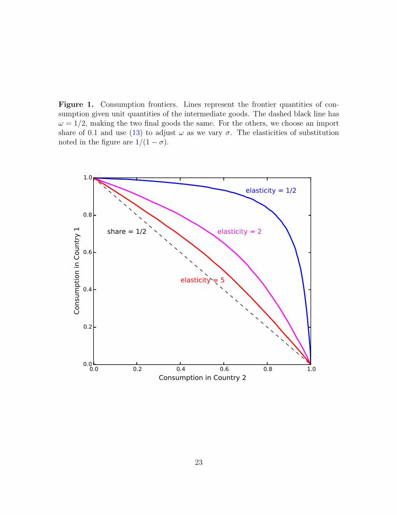
Figure 1. Consumption frontiers. Lines represent the frontier quantities of con-sumption given unit quantities of the intermediate goods. The dashed black line hasω = 1/2, making the two final goods the same. For the others, we choose an importshare of 0.1 and use (13) to adjust ω as we vary σ. The elasticities of substitutionnoted in the figure are 1/(1− σ).
0.0 0.2 0.4 0.6 0.8 1.0
Consumption in Country 2
0.0
0.2
0.4
0.6
0.8
1.0
Consu
mpti
on in C
ountr
y 1 share = 1/2
elasticity = 1/2
elasticity = 2
elasticity = 5
23
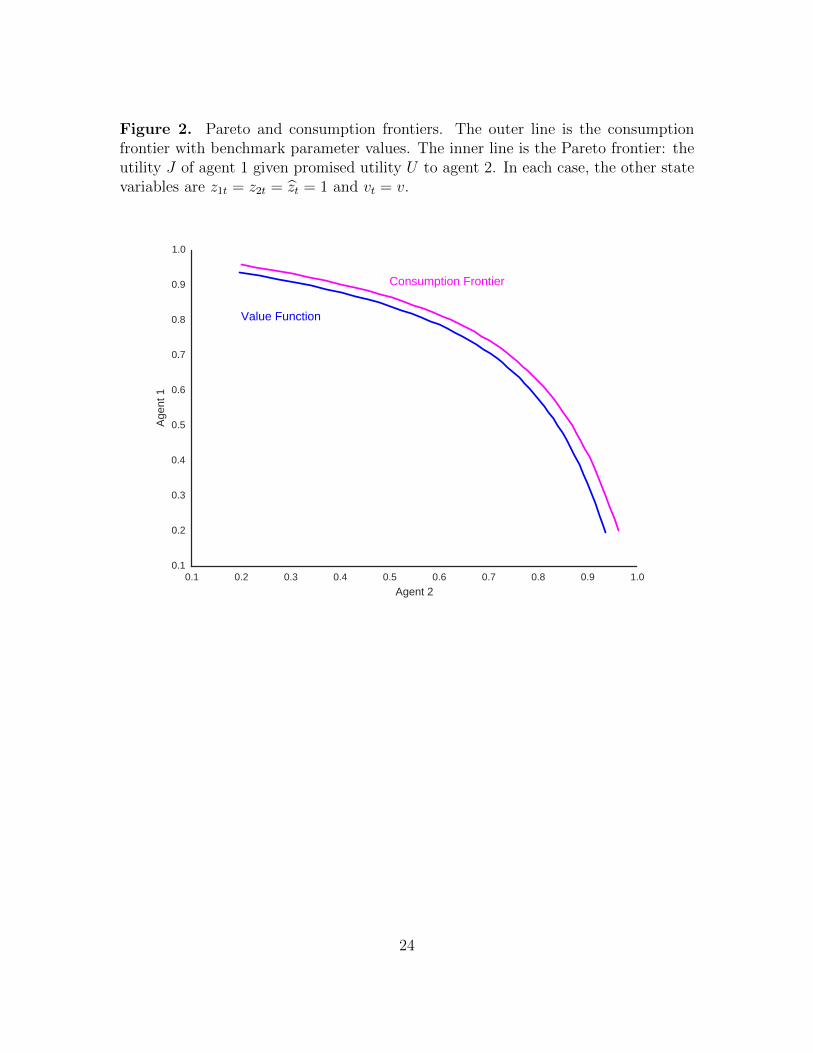
Figure 2. Pareto and consumption frontiers. The outer line is the consumptionfrontier with benchmark parameter values. The inner line is the Pareto frontier: theutility J of agent 1 given promised utility U to agent 2. In each case, the other statevariables are z1t = z2t = zt = 1 and vt = v.
0.1 0.2 0.3 0.4 0.5 0.6 0.7 0.8 0.9 1.0Agent 2
0.1
0.2
0.3
0.4
0.5
0.6
0.7
0.8
0.9
1.0
Age
nt 1
Value Function
Consumption Frontier
24

Figure 3. Dynamics of the additive and recursive Pareto weight. The two linesrepresent simulations of models with additive (α = ρ = −1) and recursive (α =−9, ρ = −1) preferences. The simulations use the same paths for exogenous statevariables. In each case, we plot log λ∗t against time.
0 1000000 2000000 3000000 4000000 5000000Time
3
2
1
0
1
2
3
Rat
io o
f Par
eto
Wei
ghts
Additive Model
Recursive Model
25

Figure 4. Risk aversion and expected changes in the Pareto weight. The lines rep-resent the expected change in log λ∗t [Et(∆ log λ∗t+1)] with three values of risk aversion1− α: 2 (additive), 10, and 50.
3 2 1 0 1 2 3
logλ ∗t
0.00006
0.00004
0.00002
0.00000
0.00002
0.00004
0.00006
E[logλ∗ t+
1]−
logλ
∗ t
Risk Aversion of 50
Risk Aversion of 10Risk Aversion of 2
26

Figure 5. Armington substitutability and expected changes in the Pareto weight.The lines represent the expected change in log λ∗t [Et(∆ log λ∗t+1)] with three valuesof the substitutability parameter σ in the Armington aggregator. The elasticities1/(1− σ) are 2/3, 1, and 2.
27

Figure 6. Intertemporal substitution and expected changes in the Pareto weight.The lines represent the expected change in log λ∗t [Et(∆ log λ∗t+1)] with three values ofthe substitutability parameter ρ in the time aggregator: −1, −0.01, and 1/3. Theycorrespond to intertemporal elasticities of substitution of 1/2, 0.99, and 3/2.
28
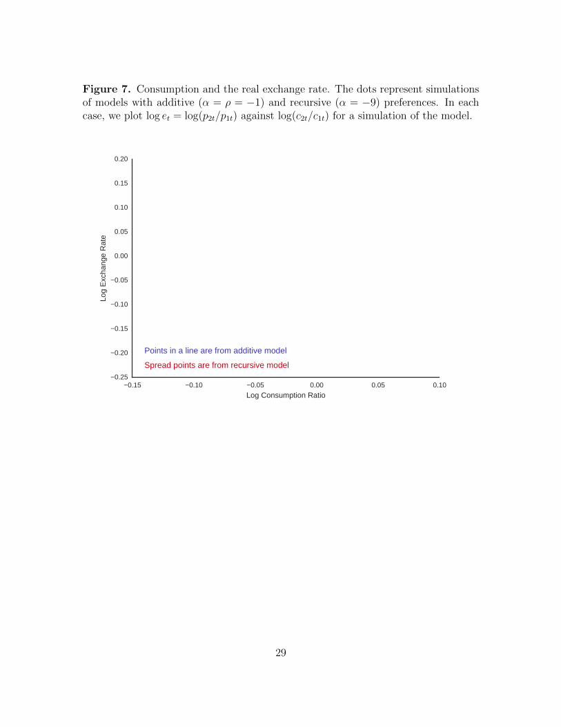
Figure 7. Consumption and the real exchange rate. The dots represent simulationsof models with additive (α = ρ = −1) and recursive (α = −9) preferences. In eachcase, we plot log et = log(p2t/p1t) against log(c2t/c1t) for a simulation of the model.
0.15 0.10 0.05 0.00 0.05 0.10Log Consumption Ratio
0.25
0.20
0.15
0.10
0.05
0.00
0.05
0.10
0.15
0.20
Log
Exc
hang
e R
ate
Points in a line are from additive model
Spread points are from recursive model
29

Figure 8. Dynamics of the real exchange rate. The lines represent autocorrelationfunctions for the real exchange rate (log et) in models with additive (α = ρ = −1)and recursive (α = −9) preferences.
0 5 10 15 20 25 30 35 40Lag (Quarters)
0.0
0.2
0.4
0.6
0.8
1.0
Aut
ocor
rela
tion
Additive
Recursive
30
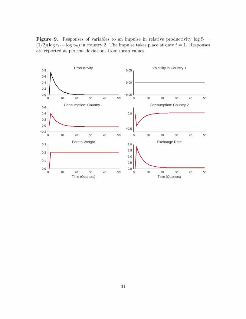
Figure 9. Responses of variables to an impulse in relative productivity log zt =(1/2)(log z1t− log z2t) in country 2. The impulse takes place at date t = 1. Responsesare reported as percent deviations from mean values.
0 10 20 30 40 500.0
0.2
0.4
0.6
0.8Productivity
0 10 20 30 40 500.05
0.00
0.05Volatility in Country 1
0 10 20 30 40 500.2
0.0
0.2
0.4
0.6Consumption: Country 1
0 10 20 30 40 50
0.5
0.0
Consumption: Country 2
0 10 20 30 40 50Time (Quarters)
0.0
0.1
0.2
0.3Pareto Weight
0 10 20 30 40 50Time (Quarters)
0.0
0.5
1.0
1.5
2.0Exchange Rate
31

Figure 10. Responses of variables to an impulse in volatility vt. The impulse takesplace at date t = 1. Responses are reported as percent deviations from mean values.
0 10 20 30 40 500.05
0.00
0.05Productivity
0 10 20 30 40 500
2
4
6
8Volatility in Country 1
0 10 20 30 40 500.0005
0.0000
0.0005
0.0010
0.0015Consumption: Country 1
0 10 20 30 40 500.0015
0.0010
0.0005
0.0000
0.0005Consumption: Country 2
0 10 20 30 40 50Time (Quarters)
0.010
0.005
0.000
0.005Pareto Weight
0 10 20 30 40 50Time (Quarters)
0.006
0.004
0.002
0.000
0.002Exchange Rate
32