SESUG 2014

1

Paper PO-147

ANALYSIS OF ZERO INFLATED LONGITUDINAL DATA USING PROC NLMIXED

Delia C Voronca, Leonard E Egede, Mulugeta Gebregziabher, Medical University of South Carolina, Charleston, SC; Ralph H. Johnson VAMC, Charleston, SC;

ABSTRACT

Commonly used parametric models may lead to erroneous inference when analyzing count or continuous data with excess of zeroes. For non-clustered data, the most commonly used models to address the issue of excess zeroes are zero inflated Poisson (ZIP), zero inflated negative binomial (ZINB), hurdle Poisson (HP) and hurdle negative binomial (HNB). Our goal is to expand these for modeling longitudinal data by developing a unified PROC NLMIXED based SAS® macro that allows for a grid search of parameter initial values to facilitate convergence. The motivating data set comes from a longitudinal study in an African American population with poorly controlled type 2 diabetes conducted at the Veterans Administration (VA) and Medical University of South Carolina (MUSC) medical centers between 2009 and 2012. A total of 256 subjects were followed for one year and measures were taken at baseline and at month 3, 6 and 12 post baseline after the subjects were randomly assigned to four treatment groups: Telephone-delivered diabetes knowledge/information, Telephone-delivered motivation/behavioral skills training intervention, Telephone-delivered diabetes knowledge/information and motivation/behavioral intervention and Usual Care. The main goal of the study was to determine the efficacy of the treatment groups in relation to the usual care group in reducing the levels of hemoglobin A1c at 12 months. We used these data to demonstrate the application of this unified SAS macro that has the capability to fit the above two part/mixture models for zero inflated and correlated count data. The macro facilitates model comparison based on fit statistics, parameter estimates with corresponding standard errors and graphs. Moreover, the proposed unified macro address the issue of convergence by finding good initial starting values for the parameters and performing a grid search for the best estimation of the standard errors corresponding to the random effects.

INTRODUCTION

Zero inflation describes data for which the number of observed zeroes is higher than what is expected from a standard Poisson distribution and often results in over-dispersion. The starting point when analyzing any count data is usually a Poisson distribution. However, this distribution cannot account for zero-inflation since its conditional mean cannot vary independently of its corresponding variance. When these issues are not properly addressed, the analysis may lead to biased estimates, underestimated standard errors and distorted test statistics of overall goodness of fit [1].To address these problems, other models have been proposed such as negative binomial [2],hurdle [3]and zero inflated models [4]. Negative binomial (NB) model accounts for over-dispersion due to heterogeneity among individuals, zero inflated Poisson (ZIP) and hurdle Poisson (HP) models account for zero inflation whereas zero inflated negative binomial (ZINB) and hurdle negative binomial (HNB) account for over-dispersion due to both heterogeneity and zero inflation. The latter two have been shown to produce more reliable inference and therefore may be the most appropriate tools when modelling count data with zero inflation [5, 6]

These models were extended to correlated data to account for correlations between repeated/clustered measures by including random effects [7-10].Different ways of extending these models with random effects were suggested. One way is to add the random effect only to the Poisson/NB part of the mixture models [7]. Another way is two add a pair of uncorrelated or correlated random effects to both parts of the mixture model [8, 10] which has proven to be more efficient. Another approach is to fit marginal versions of these models using a generalized estimating equations (GEE) approach [11].While the generalized linear mixed effects models (GLMM) is a subject/cluster specific model and inference is made at individual level, GEE is a marginal model and inference is made at population level by incorporating a dependence working correlation matrix. GLMM has less restrictive assumption for missingness and it is a more popular approach among researchers and scientists. We adopt a GLMM type of analysis for our study.

Currently, zero inflated models for cross sectional data are fitted in SAS using PROC TCOUNTREG. However, the procedure does not fit hurdle models and does not allow for random effects when dealing with longitudinal or clustered data. In order to get suggestive graphs of the predictive capability of the model the macro PROBCOUNT is used in conjunction with PROC TCOUNTREG.

The proposed unified macro uses different techniques to optimize convergence of the algorithm used for estimation, simplifies the programming syntax and provides key output that facilitates model comparison. In addition, the macro generates a graph of observed versus predicted count probabilities for simper models such as Poisson and NB but also for mixed hurdle or zero inflated models. SAS/STAT® is needed to run the proposed unified macro and all the above mentioned procedures: PROCs TCOUNTREG, GLMM and NLMIXED.

SESUG 2014

2

MODELS FOR ZERO INFLATED COUNT DATA

Multiple articles have shown that the most usual approach to model zero inflated count data assuming a Poisson distribution or using a transformation on the outcome to attain normality may lead to erroneous inference. To address the issue of zero inflation, different models have been proposed such as NB, ZIP, ZINB, HP, and HNB. However, there are no straightforward methods to fit these models in the current version of SAS 9.4. We provide a unified macro that can be used to fit these models with correlated data. The base models considered for our macro are described below and each of them can be extend by adding random effects.

The Poisson probability distribution function is given by:

With the expected mean and variance . Since the mean equals the variance, Poisson

distribution cannot account for over or under dispersion.

The NB probability distribution can be written as:

(

)

( ) ( )

(

)

Where is the over dispersion parameter. The expected mean of NB is with the corresponding

variance . As the dispersion parameter approaches zero the negative binomial reduces to a

Poison distribution.

The zero inflated models have the following general form:

( ) { ( ) ( )

( ) ( )

Where is the probability of being an excess zero and ( ) is the distribution function for a Poison or a NB. Using a

logit link to model , the first part of the zero inflated model can be interpreted as the odds of being in the

“susceptible” class versus “non-susceptible” class [Rose]. The second part models the expected number of events

condition that the individuals are in the “susceptible” class [Rose]. This is usually done using a log link.

The mean of ZIP s given by ( ) with the corresponding variance ( ) . The

mean of ZINB is given by ( ) with the corresponding variance ( ) ( ) .

Note that the variance of a zero inflated model can never exceed the mean and for this reason the ZIP and ZINB cannot accommodate under dispersion.

The hurdle models have the following general form:

( ) {

( ) ( )

Where is the probability of being a zero and ( ) is the truncated distribution function at zero i.e. ( )

with ( ) the distribution function for a Poison or a NB.

The general form of the mean of a hurdle is given by ( )

and its corresponding variance is

( ) ( )

where f is the base distribution, Poisson or NB, and are the mean and variance

of the base distribution.

Hurdle model can account for both over dispersion and under dispersion. When there is evidence of zero

inflation comparative to a standard Poisson distribution. Similarly, when there is evidence of under

dispersion. The zero inflated models can be written as a hurdle model with mixing probability

(Neelon, 2010). For this reason, zero inflated models can be considered special cases of the hurdle model.

An important issue is the conceptual framework for zero inflated and hurdle models which must be carefully considered. Even though both models assume that the data are generated by two different processes, they model the zeroes in two different ways. In this context, there can be two types of zeroes: sampling zeroes and structural zeroes. Sampling zeroes arise from subjects that are at risk but do not experience the event whereas structural zeroes arise from subjects that are not-at risk and therefore can’t experience the event [12].Hurdle models assume that all subjects are at risk and therefore all zeroes are generated by one process whereas the positive counts are part of a truncated distribution. The likelihoods corresponding to the two parts of the hurdle are separable in terms of

SESUG 2014

3

parameters being estimated and therefore it can be fit in two steps. For this reason hurdle is often considered a two part conditional model and it is easier to interpret and implement comparative to a zero inflated model. On the other hand, the zero inflated models assume the existence of both sampling and structural zeroes and the likelihoods are not separable with respect to the parameters being estimated. After separating the sampling zeroes from the structural zeroes by assuming the existence of an underlying latent class, the sampling zeroes together with the positive counts are modeled using a Poisson or a Negative Binomial distribution. Since the zeroes are thought to be generated by a mixture of two distributions corresponding to the population at risk and not at risk the zero inflated models are more naturally classified as mixture models.

ESTIMATION AND MODEL COMPARISON

When random effects are added to the fixed effects, the likelihood of the observed data becomes a marginal likelihood after integrating over the random effects. However, this marginal likelihood does not have a closed form most of the time and it needs to be approximated. The most commonly used methods for maximum likelihood (ML) integral approximation are marginal quasi likelihood (MQL), penalized maximum likelihood (PQL), linear mixed effects approximation ((LME), importance sampling, Markov Chain Monte Carlo (MCMC), Gaussian Quadrature (GQ) and adaptive Gaussian Quadrature (AGQ) center at the conditional mode of the random effect. The AGQ with one quadrature point is equivalent to Laplace approximation which is an exact approximation for liner mixed models. These methods have been compared when fitting GLMM methods and GQ and AGQ in general lead to reliable results and are better comparative to the other methods[13, 14]. The precision of the estimation increases with the number of quadrature but so does the computational time. The proposed macro uses PROC NLMIXED and therefore the estimates of the model parameters are likelihood-based. The second order derivative matrix of the likelihood function is used for estimation of parameters and standard errors [15]. PROC NLMIXED used AGQ as default method, and a first order Taylor series for integral approximation. The default maximization technique is quasi-Newton algorithm [15]. In PROC NLMIXED, the number of quadrature points can also be automatically set using the option “qpoints”. The optimal number of quadrature points suggested in the literature for the AGQ in order to increase the accuracy of the estimates is at least 5 with improved results for 10 up to 30 quadrature pints [16, 17]. Currently, the distribution of the random effects can only be normal [15].

The recommended ways to compare models for zero inflated count data is in terms of model fit are Akaike information criterion (AIC) and Bayesian information criterion (BIC) [18]. Also, a likelihood ratio test can be used for nested models such as Poisson and Hurdle or Poisson and ZIP. To determine how well a model predicts, a graph of the observed versus predictive probabilities can be very suggestive and often can help discriminate between models that appear to have the same fit.

THE UNIFIED SAS MACRO DESCRIPTION

The proposed unified SAS macro is based on PROC NLMIXED SAS 9.4 which is a procedure that fits models using a likelihood-based approach. Dummy variables need to be created for categorical covariates and data must be in long format for longitudinal data analysis. The macro comprises several positional parameters: the dependent count variable (outcome), the model type (“modeltype”), the variables included in the model (“vars”, “vars0”), a slope variable when a random slope is specified (“slope”), the input data set (“in”) and a unique identifier (“id”). Values for these parameters must be supplied otherwise the macro will generate an error. The “modeltype” can be set to Poisson, NB, ZIP, ZINB, HP or HNB. The covariates of interest supplied to “vars” or “vars0” should be separated by spaces. Also interaction is allowed by using the multiplication symbol (*). After each parameter value a comma is required. There are also a few key parameters such as the inclusion of random intercept for the count part (“c0”), random intercept for the zero part (“z0”), random slope for the count part (“c1”), correlation between the random intercepts or between the random intercept and random slope in the count part (“corr”) and plot (plot) which creates a graph of predicted versus observed probabilities. All these parameters have false default value. The title of the graph can also be changed by assigning a value to the “title” parameter and an additional parameter (“where”) allows for sub setting.

The ML approximation is done using the default method which is the adaptive Gaussian Quadrature (AGQ) [14] that has been shown to produce reliable estimates for GLMM [16] or by specifying the number of quadrature points to get a more precise estimation. When the quadrature points is fixed to one the resulting estimates are equivalent to Laplace approximation. Before any model is ran, the data is sorted on the repeated unique identifier to optimize convergence[19]. First, the macro runs the simple models with no random effects to get initial values to be used in subsequent models that include random effects. The ML for mixed /two part models with random effects is estimated on 15 quadrature points by default but it can also be changed in the macro syntax in order to increase the precision of the estimation (“qpoints”).

Since the variance of the random effects may be hard to approximate, the macro can perform a grid search on a range of values and chooses the optimal value based on the best combination. The default range was set from 0.1 to 10.1 by 1s but it can be changed in the macro syntax (the “grid” macro variable) if a different range of values is desired. The “grid” parameter can also take one value instead of a range of values. The initial values for the models with no random effects “parmsinit” and the dispersion parameter “alphainit” can be changed in the macro syntax. The default initial value for model parameters is 0 and for the dispersion parameter is 0.1.The maximum number of

SESUG 2014

4

iterations (“maxit”) to convergence is set to 500. Below are some examples on how to assign values to some of these parameters inside the macro in order to optimize convergence:

%let maxit=500; /*maximum number of allowed iterations until convergence*/

%let qpoints=%STR(qpoints=15); /*number of quadrature points for the Gaussian Quadrature algorithm is set to 15 for any type of model */

%let qpoints=%STR(); /* the default PROC NLMIXED Adaptive Gaussian Quadrature is used for any type of model*/

%let initparms=0; /*initial values for models with no random effects;*/

%let alphainit=0.1;/*dispersion parameter initial value for any type of model */

%let grid=0.1 to 10.1 by 1; /*a range of initial values for the variance of the random effects*/

%let grid=0.1; /*the initial value can be also be one number estimated from other random effects model;*/

The macro can fit simple Poisson and NB with or without random intercepts and slope that can be correlated or not, ZIP, ZINB, HP, and HNB with one or two random intercepts corresponding to the two parts that can be correlated or uncorrelated, or with both random intercept and slope in the count part only that can also be correlated or uncorrelated. Since PROC NLMIXED performance decreases with the number of random effects we have not yet extended the macro for more than three random effects [15]. The macro will select tables of interest from the usual PROC NLMIXED output such as Dimensions, Parameters (or Initial Parameters) Convergence Status, Fit Statistics and Parameter Estimates. In addition, the macro will output the total run time and a graph of predicted versus observed probability for counts.

REAL DATA EXAMPLE

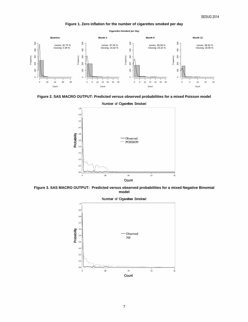
The motivating data set comes from a longitudinal study in an African American population with poorly controlled type 2 diabetes conducted at VA and MUSC centers in SC between 2008 and 2011. The study was funded by grant R01DK081121 (Egede PI) from the National Institute of Diabetes and Digestive and Kidney Diseases (NIDDK). A total of 256 subjects were followed for one year and measures were taken at baseline and at month 3, 6 and 12 post-baseline after the subjects were randomly assigned to four treatment groups: Telephone-delivered diabetes knowledge/information, Telephone-delivered motivation/behavioral skills training intervention, combined and Usual Care. The main goal of the study was to determine the efficacy of the treatment groups in relation to the usual care group in reducing the levels of hemoglobin A1C at 12 months. The average age of the sample is 57 years old with a mean BMI of 34.81. There are approximately 45% women and 55% males. We use these data to demonstrate the application of the unified SAS macro. The zero inflated count outcome used for these analyses are the number of cigarettes smoked per day. In terms of conceptual framework, both zero inflated and hurdle makes sense for the number of cigarettes smoked per day. A zero Inflated model is feasible since we can consider that some individuals are at risk (“susceptible”) of smoking but choose not to smoke for the study period and some are not at risk (“not susceptible”) because they never smoke. Also hurdle model makes sense since all people can be considered at risk for smoking. The overall mean for the number of cigarettes smoked per day is 4.57 and the corresponding variance is 20.88. The percentage of zeroes at each time point is presented in figure 1. The variance exceeds the overall mean and the percentage of zeroes is above 80% for any time point. These suggest that zero inflation is present.

In the final model we include covariates that were different between treatment groups at randomization: comorbidity, depression and foot care at baseline. We center and scale the continuous covariates, comorbidity, foot care and time, to reduce variability in the covariance matrix and optimize convergence. Also we suggest removing outliers in order to improve convergence. We create dummy variables for the categorical covariates, one for depression and three for the treatment group. The reference categories are being depressed and usual care treatment group. We assume a linear trend over time. We also introduce random effects to account for between individuals variability. We introduced random slope in the count part but the model did not improve significantly based on –2log and AIC. For simplicity and since no priory information is known about what is related to occurrence of a zero outcome we used the same set of covariates for both parts of the model. We introduce random intercepts in both parts of the model and these can be either correlated or uncorrelated.

For both the Poisson and NB for number of cigarettes smoked per day, the model is:

( )

Where is the Poisson or NB mean for subject i at time j, betas are the coefficients to be estimated and is the

random intercept such that . The same set of covariates and time treatment interactions with a random

intercept are used to model the probability for the zero part of the mixture models with a logit link:

SESUG 2014

5

( )

Where is either the probability of being a zero for a hurdle models, or the probability to be in the “non-

susceptible” class for a zero inflated model.

Below is the macro syntax for fitting a Hurdle Poisson with two uncorrelated random intercept:

%unifmacro(outcome=smokez,vars=t0_comorbsc_c depno t0_foot_c trt1 trt2 trt3 time_c

trt1*time_c trt2*time_c trt3*time_c,

vars0=t0_comorbsc_c depno t0_foot_c trt1 trt2 trt3 time_c trt1*time_c trt2*time_c

trt3*time_c , modeltype=hp, z0=true, c0=true, plot=true, title="Cigarettes smoked",

in=long, id=zsubjectcode)

RESULTS

For all models the default number of quadrature points (qpoints=15) for the SAS macro was initially used in order to get more precise estimates. The initial value for random effects variance was set to 0.1. However, when fixing the number of quadrature points the ZINB and HNB did not converge. We had to change to the default Gaussian adaptive quadrature for ZINB and HNB to reach convergence. Also, the ZIP model did not converge when the random effects variances were set to a fixed value of 0.1with adaptive Gaussian quadrature. Using the grid search with different values between 0.1 and 10.1 with an increment of 1, the convergence was reached in 58sec. After reaching convergence, we compared different models for the number of cigarettes smoked per day in terms -2log, AIC and BIC. The smallest AIC corresponds to HNB (AIC=1014.6) fallowed by ZIP and HP (AIC=1057.4, AIC=1057.8). Based on -2log or BIC we get similar results. There does not seem to be a difference between ZIP and HP in terms of model fit. The worst fit corresponds to the Poisson model with random intercept (AIC=1299.5), as expected. In terms of computational efficiency, most models take less than a minute to reach convergence after adjusting the grid search or changing the estimation method. The most computationally inefficient model was ZINB which took 3min57sec to reach convergence after using the grid search with adaptive Gaussian quadrature. Model fit results and run times are presented in Table 2. We also assess the predictive capability based on graphs of observed versus predicted probabilities. The plots suggest that the NB model predicts best the count probabilities for number of cigarettes smoked per day. The HNB model also has a good predictive capability based on the graph. We conclude that a HNB is the best model for the number of cigarettes smoked per day. The table of the beta and alpha coefficients estimates and corresponding p-values are presented in Table 3. Our analysis suggests that there is no difference over time between the trajectories associated with the four treatment groups for the hurdle part or the zero part.

CONCLUSIONS AND DISCUSSION

To sum up, correlated zero inflated count outcomes require different methods to address deviations from a standard Poisson distribution in order to get valid inference. However, current SAS procedures do not provide an easy implementation of models for zero inflated count data especially when the count outcomes are correlated and random effects are included. Convergence can become an issue especially when the initial values of the parameters are far from the truth or when too many random effects are included. The proposed unified macro addresses the issue of convergence by finding good initial starting values for the parameters and performing a grid search for the best estimation of the standard errors corresponding to the random effects. The programming syntax is greatly simplified which also avoids typing errors when programming different likelihood functions. Moreover, the macro simplifies the output by selecting important tables generated by PROC NLMIXED such as the fit statistics and parameter estimates and provides a graph of predictive versus observed probabilities that allows the user to assess the predictive capability of the model. The run time for each model is also recorded. Most models converged faster under the adaptive Gaussian Quadrature versus Gaussian quadrature with fixed number of quadrature points. Also, the grid search is a solution to reaching convergence or to improve convergence time. Using a real data example, we found that HNB is the best fit for the number of cigarettes smoked pre day based on the smallest AIC. This makes sense since HNB accounts for both over dispersion due to heterogeneity and for zero inflation which was suggested by preliminary analysis. Moreover, it is feasible to assume that all subjects are “susceptible” for smoking and hurdle model also fits well conceptually. We conclude that the proposed unified SAS macro is a useful tool for comparing models on a theoretical basis but the user should always take into account the conceptual framework when fitting two part/mixture models for zero inflated count outcomes.

SESUG 2014

6

Table 1. Model comparison for number of cigarettes smoked per day using AIC, BIC and -2log. NB=Negative Binomial, ZIP=Zero Inflate Poisson, ZINB=Zero Inflate Negative Binomial, HP=Hurdle Poisson, HNB=Hurdle

Negative Binomial

Poisson NB ZIP ZINB HP HNB

-2log 1275.5 1162.0 1009.4 1081.3 1009.8 964.6

AIC 1299.5 1188.0 1057.4 1131.3 1057.8 1014.6

BIC 1342.0 1234.1 1142.5 1220.0 1142.9 1103.2

Run time 8sec 42sec 58sec 3min57 20sec 1min1sec

Table 2. SAS MACRO OUTPUT: Beta and Alpha estimates for HNB with random intercepts in both parts of the model. Betas represent the coefficients for count part whereas alphas are coefficients for the zero part.

Parameter Estimates

Parameter Estimate Standard Error DF t Value Pr > |t| Alpha Lower Upper Gradient

b0 1.6347 0.3302 254 4.95 <.0001 0.05 0.9844 2.2849 0.000382

b1 0.1724 0.1930 254 0.89 0.3726 0.05 -0.2077 0.5524 -0.00111

b2 0.1609 0.3292 254 0.49 0.6254 0.05 -0.4875 0.8093 0.000454

b3 -0.1306 0.1506 254 -0.87 0.3868 0.05 -0.4273 0.1661 -0.00131

b4 -0.2684 0.3993 254 -0.67 0.5020 0.05 -1.0549 0.5180 0.000294

b5 -0.03492 0.4292 254 -0.08 0.9352 0.05 -0.8802 0.8103 0.000238

b6 0.07019 0.4347 254 0.16 0.8719 0.05 -0.7859 0.9263 -0.00016

b7 -0.01252 0.02168 254 -0.58 0.5641 0.05 -0.05521 0.03017 0.000488

b8 -0.04677 0.03302 254 -1.42 0.1579 0.05 -0.1118 0.01825 -0.00271

b9 -0.00482 0.04087 254 -0.12 0.9062 0.05 -0.08530 0.07566 -0.00038

b10 0.04858 0.03024 254 1.61 0.1094 0.05 -0.01098 0.1081 0.001307

a0 10.9643 1.9186 254 5.71 <.0001 0.05 7.1859 14.7428 0.000311

a1 -0.1328 0.6561 254 -0.20 0.8398 0.05 -1.4249 1.1593 0.000277

a2 0.1967 1.6001 254 0.12 0.9023 0.05 -2.9544 3.3478 0.000326

a3 0.2812 0.6855 254 0.41 0.6819 0.05 -1.0687 1.6312 -0.00039

a4 -0.2467 1.9032 254 -0.13 0.8969 0.05 -3.9947 3.5013 0.000062

a5 0.8894 2.1033 254 0.42 0.6728 0.05 -3.2528 5.0316 -0.00014

a6 1.4520 2.4221 254 0.60 0.5494 0.05 -3.3179 6.2220 0.000108

a7 -0.01802 0.1566 254 -0.12 0.9085 0.05 -0.3264 0.2904 0.002738

a8 -0.02641 0.1986 254 -0.13 0.8943 0.05 -0.4176 0.3648 0.00072

a9 0.1590 0.2019 254 0.79 0.4317 0.05 -0.2386 0.5565 0.000486

a10 0.3213 0.3052 254 1.05 0.2936 0.05 -0.2799 0.9224 0.001297

alpha 0.1110 0.03506 254 3.17 0.0017 0.05 0.04192 0.1800 -0.00234

sigma2b 0.6791 0.2035 254 3.34 0.0010 0.05 0.2783 1.0799 -0.00026

sigma2a 522.03 230.45 254 2.27 0.0243 0.05 68.1876 975.88 -2.86E-6

SESUG 2014

7

Figure 1. Zero inflation for the number of cigarettes smoked per day

Figure 2. SAS MACRO OUTPUT: Predicted versus observed probabilities for a mixed Poisson model

Figure 3. SAS MACRO OUTPUT: Predicted versus observed probabilities for a mixed Negative Binomial model

Baseline

Count

Fre

quency

0 20 40 60 80

0100

200

300

400

500

zeroes: 82.75 %missing: 0.39 %

Month 3

Count

Fre

quency

0 5 10 15 20 25 300

100

200

300

400

500

zeroes: 87.04 %missing: 15.62 %

Month 6

Count

Fre

quency

0 5 10 15 20 25 30

0100

200

300

400

500

zeroes: 86.08 %missing: 24.22 %

Month 12

Count

Fre

quency

0 5 10 15 20

0100

200

300

400

500

zeroes: 86.63 %missing: 26.95 %

Cigarettes Smoked per Day

SESUG 2014

8

Figure 4. SAS MACRO OUTPUT: Predicted versus observed probabilities for a mixed Hurdle Negative Binomial model

SESUG 2014

9

Source Code

*************************MACRO USING PROC NLMIXED FOR COUNT

DATA**************************;

***********MACRO TEMPLATE from Gary Bonin: best Practices and Advanced tips and

Techniques For SAS macro programming*********;

dm log 'clear';*clear the log before running the macro;

options mcompilenote=all;*display macro compile information;

* Refer: macros(xxxxxxxx)

* Function: GLMM for zero inflated counts

*

*

* Notes: must have dummy variables for all categorical variables;

* Notes: when using the macro make sure to include comes between the parameters

otherwise errors will be generated;

*

* (C) Copyright 2010 MUSC, Dept. Of Biostatistics

*

* Revision history:

*

* Date Name Description of Change in order to keep track of changes/reasons for

changes

* -------- -------------- --------------------------------------------------

* 06/24/2014 Delia Voronca Initial version.

* 06/24/2014 Delia Voronca modify macro to read initial parameter values from

complementary models.

* 07/14/2014 Delia Voronca modify macro to add random slopes in the count part

correated and uncorrelated;

* 07/15/2014 use the _est data set to red new parameters values;

* 08/17/2014 Delia Voronca add the graph options for predicted versus observed

probabilities;

************************************************************************* */

options symbolgen mlogic mprint ;

%macro unifmacro

( outcome= /* 1st positional parameter: the count outcome of interest*/

, modeltype= /* 2nd positional parameter: the type of the model Poisson, NB, ZIP,

ZINP, HP, HNB*/

, vars= /* 3rd positional parameter: variables included in the count model ,

default just intercept*/

, vars0= /* 4th positional parameter: variables included in the zero part model,

used only if 2 part model else error*/

, slope= /* 5th positional parameter: variables necessary if we want to include

random slope in the count model;*/

, title= /* 6th positional parameter: title for the plot */

, c0=FALSE /*1st keyword parameter: random intercept in the Poisson, NB or count

part*/

, c1=FALSE /*2nd keyword parameter: random slope in the Poisson, NB or count part*/

, z0=FALSE /*3rd keyword parameter: random intercept in the zero part, used only

for ZIP ZINB HP HNB*/

, corr=FALSE /*4th keyword parameter: correlation between two random intercepts or

correlation between random slope and random intercept*/

, plot=FALSE /*5th keyword parameter: plot predicted versus observed

probabilities*/

, in= /* input file name */

, id= /*unique identifier for independent observations, needed for sorting to

improve convergence*/

, where= /* limit on the input file */

);

*record the time it takes to run the macro;

%let ts_start = %sysfunc( datetime(), 16. ) ;

%let now = %sysfunc( putn( &ts_start, datetime16. ) ) ;

%put INFO: &sysmacroname: &now: Starting execution. ;

*make all input parameters uppercase to avoid errors;

%let c0=%UPCASE(&c0);

SESUG 2014

10

%let z0=%UPCASE(&z0);

%let c1=%UPCASE(&c1);

%let corr=%UPCASE(&corr);

%let plot=%UPCASE(&plot);

%let modeltype=%UPCASE(&modeltype);

*set some default values for PROC NLMIXED;

%let maxit=500; /*maximum number of allowed iterations until convergence*/

%let qpoints=%STR(qpoints=10); /*number of quadrature points for the adaptive

Gaussian Quadtrature algorithm*/

%let initparms=0.1; /*initial values for models with no random effects;*/

%let alphainit=0.1;

%let grid=0.1 to 10.1 by 1;

*get the variables included in the count/zero model and initialize default all are

0;

%let modelvars = b0; *count part: this denotes the intercept which is in the model

by default;

%let modelvars0 = a0; *zero part: this denotes the intercept which is in the model

by default;

%let parmsb = b0=&initparms; *count part: used for initial values of the model

parameters;

%let parmsa = a0=&initparms; *zero part: used for initial values of the model

parameters;

%let numvar=%numargs(&vars);

%let numvar0=%numargs(&vars0);

%let randompart=;

*initialize the NB parameters;

%let m = 1/alpha; *alpha is the dispersion parameter, as it goes to zero the NB

converges to Poisson;

%let p = 1/(1+mu*alpha);

*output error is some of the mandatory key input parameters are not supplied;

%if %length(&outcome)=0 %then %do;

%put ERROR: No outcome variable supplied;

%return;

%end;

%if %length(&modeltype)=0 %then %do;

%put ERROR: No model type supplied;

%return;

%end;

%if %length(&in)=0 %then %do;

%put ERROR: No dataset supplied;

%return;

%end;

%if %length(&id)=0 %then %do;

%put ERROR: No id variable supplied;

%return;

%end;

%if &z0=TRUE and (&modeltype=POISSON or &modeltype=NB) %then %do;

%put ERROR: The model you are fitting does not have a zero part;

%return;

%end;

%if %length(&slope)=0 and &c1=TRUE %then %do;

%put ERROR: No slope variable supplied;

%return;

%end;

/*check the where condition;*/

%if %length(&where) ne 0 %then

%let where=where &where ;

/*select none or specific output to be displayed;*/

%if &z0=TRUE or &c0=TRUE or &c1=TRUE %then

%let opt=ods exclude all;

%else

SESUG 2014

11

%let opt=ods select Dimensions Parameters ConvergenceStatus FitStatistics

ParameterEstimates;

/*sort data set by unique identifier in order to improve convergence;*/

proc sort data=&in; by &id; run;

/*record model parameters and initialize all with 0;

*count model, default just intercept;

*for any type of model we name coefficients for the covariates specified by vars;*/

%do i=1 %to &numvar;

%let thisvar = %scan(&vars, &i, %str( ));

%let modelvars = &modelvars + b&i*&thisvar;/*beta coefficients for counts;*/

%let parmsb = &parmsb b&i=&initparms;/*initial starting values;*/

%end;

%do j=1 %to &numvar0;

%let thisvar0 = %scan(&vars0, &j, %str( ));

%let modelvars0 = &modelvars0 + a&j*&thisvar0;/*alpha coefficients for

zeroes;*/

%let parmsa = &parmsa a&j=&initparms;/*initial starting values;*/

%end;

%if &modeltype=POISSON or &modeltype=NB %then %do;

%let parms = &parmsb;

%end;

%else %if &modeltype=ZIP or &modeltype=ZINB or &modeltype=HP or &modeltype=HNB

%then %do;

%let parms = &parmsb &parmsa;

%end;

/*MODELS WITH NO RANDOM EFFECTS;

*SIMPLE MODELS: POISSON AND NB;*/

%if &modeltype=POISSON or &modeltype=NB %then %do;

%if &modeltype=POISSON %then %do;

%let model= poisson(mu);

%end;

%else %if &modeltype=NB %then %do;

%let parms= &parms alpha=&alphainit; /*initialize dispersion parameter

with 1;*/

%let model= negbin(&m,&p);

%end;

&opt;

proc nlmixed data = &in maxit=&maxit;

&where;

parms &parms;

mu = exp(&modelvars);

model &outcome ~ &model;

predict mu out=means;

ods output "Parameter Estimates"=_est;

run;

%end;

/*TWO PART MODELS: ZIP ZINB HP HNB;

*we need to write the likelihood functions;*/

/*Introduction to SAS. UCLA: Statistical Consulting Group.

from http://www.ats.ucla.edu/stat/sas/notes2/ (accessed November 24, 2007).*/

%else %if &modeltype=ZIP or &modeltype=ZINB or &modeltype=HP or &modeltype=HNB

%then %do;

%if &modeltype=ZIP %then %do;

%let ll0 = log(prob0 + (1 - prob0)*exp(-mu));

%let ll1 = &outcome*log(mu) + log(1 - prob0) - mu - lgamma(&outcome + 1);

%end;

%else %if &modeltype=ZINB %then %do;

%let ll0 = log(prob0 + (1 - prob0)*((&p)**(&m)));

%let ll1 = log(1-prob0) + log(gamma(&m + &outcome)) - log(gamma(&outcome

+ 1))

SESUG 2014

12

- log(gamma(&m)) + &m*log(&p) + &outcome*log(1-&p);

%let parms= &parms alpha=&alphainit;

%end;

%else %if &modeltype=HP %then %do;

%let ll0=log(prob0);

%let ll1 = &outcome*log(mu) + log(1-prob0) - mu - lgamma(&outcome + 1) -

log(1-exp(-mu));

%end;

%else %if &modeltype=HNB %then %do;

%let ll0=log(prob0);

%let ll1 = log(1-prob0) + log(gamma(&m + &outcome)) - log(gamma(&outcome

+ 1))

- log(gamma(&m)) + &m*log(&p) + &outcome*log(1-&p) -

log(1-(&p)**(&m));

%let parms= &parms alpha=&alphainit;

%end;

&opt;

proc nlmixed data = &in maxit=&maxit ;

&where;

parms &parms;

logit0 = &modelvars0;

prob0 = 1 / (1 + exp(-logit0));

mu = exp(&modelvars);

if &outcome = 0 then

ll = &ll0;

else

ll = &ll1;

model &outcome ~ general(ll);

predict prob0 out=probs;

predict mu out=means;

ods output "Parameter Estimates"=_est ; /*store initial estimates;*/

run;

%end;

/*MODELS THAT HAVE RANDOM INTERCEPTS;*/

%if &z0=FALSE and &c0=FALSE and &c1=FALSE %then %goto exit;/*stop execution if

there are no random effects specified;*/

%else %do;

/*get initial values from the models with no random effects;*/

%let dsid=%sysfunc(open(_est));

%let num=%sysfunc(attrn(&dsid,nlobs));

%let rc=%sysfunc(close(&dsid));

%if &modeltype=NB or &modeltype=ZINB or &modeltype=HNB %then

%let num=%eval(&num-1);

%let parmsnew=;

%do i=1 %to %eval(&num);

data _NULL_;

set _est (firstobs=&i obs=&i);

call symput ('init_est', Estimate);

call symput ('label_est', Parameter);

run;

%let parmsnew=&parmsnew &label_est=&init_est ;

%end;

%if &modeltype=NB or &modeltype=ZINB or &modeltype=HNB %then

%let parmsnew=&parmsnew alpha=&alphainit ;/* if alpha too large from previous

estimation model may not converge;*/

%end;

/*no random slope;*/

%if &c1=FALSE %then %do;

/*just random intercept in the count part;*/

%if &c0=TRUE and &z0=FALSE %then %do;

SESUG 2014

13

%let parmsnew= &parmsnew sigma2b=&grid; /*we fix sigma2b because if too

large model may not converge;*/

%let modelvars=&modelvars + c0;

%let randompart= %str(random c0 ~ normal(0, sigma2b) subject=&id;);

%end;

/*just random intercept in the zero part;*/

%else %if &c0=FALSE and &z0=TRUE %then %do;

%let parmsnew= &parmsnew sigma2a=&grid; /*we fix sigma2a because if too

large model may not converge;*/

%let modelvars0=&modelvars0 + z0;

%let randompart= %str(random z0 ~ normal(0, sigma2a) subject=&id;);

%end;

/*uncorrelated random intercepts in the zero and count part;*/

%else %if &corr = FALSE and (&c0=TRUE and &z0=TRUE) %then %do;

%let parmsnew= &parmsnew sigma2b=&grid sigma2a=&grid; /*we fix sigma

because if too large model may not converge;*/

%let modelvars=&modelvars + c0;

%let modelvars0=&modelvars0 + z0;

%let randompart= %str(random z0 c0 ~ normal([0, 0], [sigma2a, 0,

sigma2b]) subject=&id;);

%end;

/*correlated random intercepts in the zero and count part;*/

%else %if &corr = TRUE and (&c0=TRUE and &z0=TRUE) %then %do;

%let parmsnew= &parmsnew sigma2b=&grid sigma2a=&grid cov=-0.2 to 0.2 by

0.1;

%let modelvars=&modelvars + c0;

%let modelvars0=&modelvars0 + z0;

%let randompart= %str(random z0 c0 ~ normal([0, 0], [sigma2a, cov,

sigma2b]) subject=&id;);

%end;

/*address typing errors;*/

%else %do;

%put ERROR: The random effects and correlation can take only "TRUE" or

"FALSE" value.;

%return;

%end;

%end;

/*random slope;

*currently allowed only for the count part and no random intercept in the zero

part;*/

%else %if &c1=TRUE %then %do;

/*just random slope;*/

%if &c0=FALSE %then %do;

%let modelvars=&modelvars + c1*&slope;

%let parmsnew= &parmsnew sigma2b1=&grid;

%let randompart=%str(random c1 ~ normal(0, sigma2b1) subject=&id;);

%end;

/*uncorrelated random slope and random intercept;*/

%else %if &c0=TRUE and &corr=FALSE %then %do;

%let modelvars=&modelvars +c0+ c1*&slope;

%let parmsnew= &parmsnew sigma2b=&grid sigma2b1=&grid;

%let randompart=%str(random c0 c1 ~ normal([0, 0], [sigma2b, 0,

sigma2b1]) subject=&id;);

%end;

/*correlated random slope and random intercept;*/

%else %if &c0=TRUE and &corr=TRUE %then %do;

%let modelvars=&modelvars +c0+ c1*&slope;

%let parmsnew= &parmsnew sigma2b=&grid sigma2b1=&grid cov1=-0.2 to 0.2 by

0.1;

%let randompart=%str(random c0 c1 ~ normal([0, 0], [sigma2b, cov1,

sigma2b1]) subject=&id;);

%end;

%end;

%else %do;

/*uncorrelated random slope and intercepts in both parts of the model*/

%if &c0=TRUE and &z0=TRUE and &corr=FALSE %then %do;

SESUG 2014

14

%let modelvars0=&modelvars0 + z0;

%let modelvars=&modelvars +c0+ c1*&slope;

%let parmsnew= &parmsnew sigma2a=&grid sigma2b=&grid sigma2b1=&grid;

%let randompart=%str(random c0 c1 z0~ normal([0, 0, 0], [sigma2b, 0,

sigma2b1, 0, 0, sigma2a]) subject=&id;);

%end;

%end;

/*run models with random effects;*/

%if &modeltype=POISSON or &modeltype=NB %then %do;

ods select Dimensions Parameters ConvergenceStatus FitStatistics

ParameterEstimates;

proc nlmixed data = &in &qpoints maxit=&maxit;

&where;

parms &parmsnew;

mu = exp(&modelvars);

model &outcome ~ &model;

&randompart

predict mu out=means;

ods output "Parameter Estimates"=_est ;

run;

%end;

%else %if &modeltype=ZIP or &modeltype=ZINB or &modeltype=HP or &modeltype=HNB

%then %do;

ods select Dimensions Parameters ConvergenceStatus FitStatistics

ParameterEstimates;

proc nlmixed data = &in &qpoints maxit=&maxit;

&where;

parms &parmsnew;

logit0 = &modelvars0;

prob0 = 1 / (1 + exp(-logit0));

mu = exp(&modelvars);

if &outcome = 0 then

ll = &ll0;

else

ll = &ll1;

model &outcome ~ general(ll);

&randompart

predict prob0 out=probs;

predict mu out=means;

ods output "Parameter Estimates"=_est ;

run;

%end;

%exit:

%let ts_stop = %sysfunc( datetime(), 16. ) ;

%let after = %sysfunc( putn( &ts_stop, datetime16. ) ) ;

%put INFO: &sysmacroname: &now: Starting execution. ;

%put INFO: &sysmacroname: &after: End execution. ;

/*record the run time;*/

data _time;

begin=input("&now", datetime16.);

end=input("&after",datetime16.) ;

time=end-begin;

format time time. begin datetime16. end datetime16.;

run;

proc print data=_time ; run;

/*plot predicted and observed probabilities;*/

%if &plot=TRUE %then %do;

title "&title";

%predprob(_est, means, probs);

title ;

%end;

%mend;

SESUG 2014

15

%* This macro was developed by Carrie Wager,Programmer,Channing Laboratory 1990;

%* Modified AMcD 1993, e hertzmark 1994 and L Chen 1996;

%* Use this macro to read the interraction terms;

%macro numargs(arg, delimit);

%if %quote(&arg)= %then %do;

0

%end;

%else %do;

%let n=1;

%do %until (%qscan(%quote(&arg), %eval(&n), %str( ))=%str());

%let n=%eval(&n+1);

%end;

%eval(&n-1)

%end;

%mend numargs;

%*macro to generate plot for predicted versus observed probabilities;

%*we extend the capabilities of PROBCOUNT macro to hurdle models and

to repeated measures by using predicted count generated by PROC NLMIXED;

%macro predprob(estdata, meansdata, probs);

*store the alpha estimate for NB models;

data _NULL;

set &estdata;

call symput('_alpha', Estimate);

where parameter="alpha";

run;

*get observed probabilities/proportions for each count category;

ods exclude all;

proc freq data=&in;

tables &outcome/out=_pobs;

run;

data _pobs;

set _pobs;

percent=percent/100;

run;

proc sql;

create table _maxcount as

select max(&outcome) as _maxcount from _pobs;

run;

data _NULL;

set _maxcount;

call symput('_maxcount', _maxcount);

run;

*get predicted probabilities for each subject;

data &meansdata;

set &meansdata;

keep &id &outcome pred;

run;

data &meansdata;

set &meansdata;

n=_N_;

if &outcome=. then indzero=.;

else if &outcome=0 then indzero=1;

else if &outcome ne 0 then indzero=0;

label pred="Predicted Mean";

run;

%if (&modeltype=ZIP or &modeltype=ZINB or &modeltype=HP or &modeltype=HNB) %then

%do;

data &probs;

set &probs;

keep &id &outcome pred;

rename pred=prob0;

run;

data &probs;

set &probs;

SESUG 2014

16

n=_N_;

label prob0="Probability of Zero";

run;

proc sort data=&meansdata; by n; run;

proc sort data=&probs; by n; run;

data predicted;

merge &meansdata &probs; by n;

drop n;

run;

%end;

%else %do;

data predicted;

set &meansdata;

drop n;

run;

%end;

data predicted;

set predicted;

%if (&modeltype=POISSON or &modeltype=ZIP) %then %do;

pcount=exp(-pred)*(pred**&outcome)/gamma(&outcome+1);*POISSON PDF;

%end;

%else %if (&modeltype=NB or &modeltype=ZINB) %then %do;

pcount=(gamma(&outcome+1/&_alpha)*(1/(1+&_alpha*pred))**(1/&_alpha)*(pred/(1/&_

alpha+pred))**&outcome)/(gamma(&outcome+1)*gamma(1/&_alpha));*NB PDF;

%end;

%else %if (&modeltype=HP) %then %do;

pcount=exp(-pred)*(pred**&outcome)/(gamma(&outcome+1)*(1-exp(-

pred)));*TRUNCATED POISSON PDF;

%end;

%else %if (&modeltype=HNB) %then %do;

pcount=(gamma(&outcome+1/&_alpha)*(1/(1+&_alpha*pred))**(1/&_alpha)*(pred/(1/&_

alpha+pred))**&outcome)/(gamma(&outcome+1)*gamma(1/&_alpha)*(1-

(1/(1+&_alpha*pred))**(1/&_alpha)));*TRUCATED NB PDF;

%end;

run;

data predicted;

set predicted;

%if (&modeltype=POISSON or &modeltype=NB) %then %do;

predprob=pcount;

%end;

%else %if (&modeltype=ZIP or &modeltype=ZINB) %then %do ;

predprob=indzero*prob0 +(1-prob0)*pcount;

%end;

%else %if (&modeltype=HP or &modeltype=HNB) %then %do;

predprob=prob0**indzero*((1-prob0)*pcount)**(1-indzero);

%end;

run;

*compute the average predicted probability for each count across all individuals;

proc sort data=predicted;by &outcome; run;

ods exclude all;

proc means data=predicted;

by &outcome;

var predprob;

output out=_ppred;

run;

data _ppred;

set _ppred;

where _STAT_="MEAN";

run;

proc sort data=_pobs; by &outcome;run;

proc sort data=_ppred; by &outcome;run;

data _mprob;

merge _pobs _ppred;

by &outcome;

run;

*graph;

*use PROBCOUNT SAS MACRO results section: http://support.sas.com/kb/26/161.html */

SESUG 2014

17

symbol1 v=none i=join c=black w=2; /* observed */

symbol2 v=none i=join c=green; /* model*/

axis1 label=(angle=90 font=swissb "Probability")

order=0 to 1 by .1 minor=none;

axis2 label=(font=swissb "Count") order=0 to &_maxcount minor=none;

legend1 position=(middle center inside) mode=protect across=1

label=("Models:") offset=(,8 pct) frame

value=("Observed" "&modeltype");

ods exclude none;

proc gplot data=_mprob;

plot percent*&outcome=1 predprob*&outcome=2 / overlay vaxis=axis1 haxis=axis2

legend=legend1;

run;

quit;

%mend predprob;

SESUG 2014

18

REFERENCES

1. Atkins, D.C. and R.J. Gallop, Rethinking how family researchers model infrequent outcomes: a tutorial on count regression and zero-inflated models. J Fam Psychol, 2007. 21(4): p. 726-35.

2. P.R., M., Essai d'analyses ur les jeux de hazards. 1714.

3. Mullahy, J., Specification and testing of some modified count data m. 1986.

4. Lambert, D., Zero-Inflated Poisson Regression, with an Application to Defects in Manufacturing. Technometrics, 1992. 34(1): p. 1-14.

5. Atkins, D.C., et al., A tutorial on count regression and zero-altered count models for longitudinal substance use data. Psychol Addict Behav, 2013. 27(1): p. 166-77.

6. Rose, C.E., On the Use of Zero-Inflated and Hurdle Models for Modeling Vaccine Adverse Event Count Data. Journal of Biopharmaceutical Statistics, 2006. . 16(4): p. p. 463-481.

7. Hall, D.B., Zero-inflated Poisson and binomial regression with random effects: a case study. Biometrics, 2000. 56(4): p. 1030-9.

8. Min, Y., & Agresti, A., Random effect models for repeated measures of zero-inflated count data. . Statistical Modelling, 2005. 5.

9. Molenberghs, G., & Verbeke, G. , Models for discrete longitudinal data. New York: Springer, 2005.

10. Yau, K.K., A.H. Lee, and P.J. Carrivick, Modeling zero-inflated count series with application to occupational health. Comput Methods Programs Biomed, 2004. 74(1): p. 47-52.

11. Dobbie , W., Modeling correlated zero-inflated count data; . Australian and New Zealand Journal of Statistics 2001.

12. Baughman, A.L., Mixture model framework facilitates understanding of zero-inflated and hurdle models for count data. J Biopharm Stat, 2007. 17(5): p. 943-6.

13. Aitkin, M., A General Maximum Likelihood Analysis of Variance Components in Generalized Linear Models. Biometrics, 1999. 55(1): p. 117-128.

14. Pinheiro, J.C. and D.M. Bates, Approximations to the log-likelihood function in the nonlinear mixed-effects model. Journal of computational and Graphical Statistics, 1995. 4(1): p. 12-35.

15. Wolfinger, R.D. Fitting nonlinear mixed models with the new NLMIXED procedure. in Proceedings of the 24th Annual SAS Users Group International Conference (SUGI 24). 1999.

16. Liu, Q. and D.A. Pierce, A Note on Gauss-Hermite Quadrature. Biometrika, 1994. 81(3): p. 624-629.

17. Rabe-Hesketh, S., A. Skrondal, and A. Pickles, Reliable estimation of generalized linear mixed models using adaptive quadrature. The Stata Journal, 2002. 2(1): p. 1-21.

18. Vonesh, E.F., Generalized linear and nonlinear models for correlated data: theory and applications using SAS. 2012: SAS Institute.

19. Kiernan, K., J. Tao, and P. Gibbs. Tips and strategies for mixed modeling with SAS/STAT® procedures. in SAS Global Forum. 2012.

CONTACT INFORMATION

Your comments and questions are valued and encouraged. Contact the author at:

Name: Delia Voronca Enterprise: MUSC Address: 135 Cannon Street City, State ZIP: Charleston, 29425 Work Phone: 8438761578 E-mail: voronca@musc.edu

SAS and all other SAS Institute Inc. product or service names are registered trademarks or trademarks of SAS Institute Inc. in the USA and other countries. ® indicates USA registration.

Other brand and product names are trademarks of their respective companies.