Package 'Luminescence' - The Comprehensive R Archive Network

Package ‘Luminescence’June 30, 2017

Type Package

Title Comprehensive Luminescence Dating Data Analysis

Version 0.7.5

Date 2017-06-30

Author Sebastian Kreutzer [aut, trl, cre, dtc],Michael Dietze [aut],Christoph Burow [aut, trl, dtc],Margret C. Fuchs [aut],Christoph Schmidt [aut],Manfred Fischer [aut, trl],Johannes Friedrich [aut],Norbert Mercier [ctb],Rachel K. Smedley [ctb],Claire Christophe [ctb],Antoine Zink [ctb],Julie Durcan [ctb],Georgina King [ctb, dtc],Anne Philippe [ctb],Guillaume Guerin [ctb],Markus Fuchs [ths]

Maintainer Sebastian Kreutzer <[email protected]>

Description A collection of various R functions for the purpose of Luminescencedating data analysis. This includes, amongst others, data import, export,application of age models, curve deconvolution, sequence analysis andplotting of equivalent dose distributions.

Contact Package Developers <[email protected]>

License GPL-3

BugReports https://github.com/R-Lum/Luminescence/issues

Depends R (>= 3.3.2), utils, magrittr (>= 1.5)

LinkingTo Rcpp (>= 0.12.9), RcppArmadillo (>= 0.7.600.1.0)

Imports bbmle (>= 1.0.18), data.table (>= 1.10.0), httr (>= 1.2.1),matrixStats (>= 0.51.0), methods, minpack.lm (>= 1.2-1), raster

1

https://github.com/R-Lum/Luminescence/issues

2

(>= 2.5-8), readxl (>= 0.1.1), shape (>= 1.4.2), parallel, XML(>= 3.98-1.5), zoo (>= 1.7-14)

Suggests RLumShiny (>= 0.1.1), RLumModel (>= 0.1.2), plotly (>=4.5.6), rmarkdown (>= 1.3), rjags (>= 4-6), coda (>= 0.19-1),pander (>= 0.6.0), rstudioapi (>= 0.6), testthat (>= 1.0.2),devtools (>= 1.12.0)

URL https://CRAN.R-project.org/package=Luminescence

Collate 'Analyse_SAR.OSLdata.R' 'CW2pHMi.R' 'CW2pLM.R' 'CW2pLMi.R''CW2pPMi.R' 'Luminescence-package.R' 'PSL2Risoe.BINfileData.R''RcppExports.R' 'replicate_RLum.R' 'RLum-class.R''smooth_RLum.R' 'names_RLum.R' 'structure_RLum.R''length_RLum.R' 'set_RLum.R' 'get_RLum.R''RLum.Analysis-class.R' 'RLum.Data-class.R' 'bin_RLum.Data.R''RLum.Data.Curve-class.R' 'RLum.Data.Image-class.R''RLum.Data.Spectrum-class.R' 'RLum.Results-class.R''Risoe.BINfileData2RLum.Analysis.R''Risoe.BINfileData2RLum.Data.Curve.R' 'set_Risoe.BINfileData.R''get_Risoe.BINfileData.R' 'RisoeBINfileData-class.R''Second2Gray.R' 'analyse_FadingMeasurement.R''analyse_IRSAR.RF.R' 'analyse_SAR.CWOSL.R' 'analyse_SAR.TL.R''analyse_baSAR.R' 'analyse_pIRIRSequence.R''analyse_portableOSL.R' 'app_RLum.R' 'apply_CosmicRayRemoval.R''apply_EfficiencyCorrection.R' 'calc_AliquotSize.R''calc_AverageDose.R' 'calc_CentralDose.R' 'calc_CommonDose.R''calc_CosmicDoseRate.R' 'calc_FadingCorr.R' 'calc_FastRatio.R''calc_FiniteMixture.R' 'calc_FuchsLang2001.R''calc_HomogeneityTest.R' 'calc_IEU.R' 'calc_Kars2008.R''calc_MaxDose.R' 'calc_MinDose.R' 'calc_OSLLxTxRatio.R''calc_SourceDoseRate.R' 'calc_Statistics.R''calc_TLLxTxRatio.R' 'calc_ThermalLifetime.R' 'calc_gSGC.R''convert_BIN2CSV.R' 'convert_Daybreak2CSV.R''convert_PSL2CSV.R' 'convert_XSYG2CSV.R''extract_IrradiationTimes.R' 'fit_CWCurve.R' 'fit_LMCurve.R''get_Layout.R' 'get_Quote.R' 'get_rightAnswer.R' 'github.R''install_DevelopmentVersion.R' 'internal_as.latex.table.R''internals_RLum.R' 'merge_RLum.Analysis.R''merge_RLum.Data.Curve.R' 'merge_RLum.R' 'merge_RLum.Results.R''merge_Risoe.BINfileData.R' 'methods_DRAC.R' 'methods_RLum.R''model_LuminescenceSignals.R' 'plot_AbanicoPlot.R''plot_DRTResults.R' 'plot_DetPlot.R''plot_FilterCombinations.R' 'plot_GrowthCurve.R''plot_Histogram.R' 'plot_KDE.R' 'plot_NRt.R''plot_RLum.Analysis.R' 'plot_RLum.Data.Curve.R''plot_RLum.Data.Image.R' 'plot_RLum.Data.Spectrum.R''plot_RLum.R' 'plot_RLum.Results.R' 'plot_RadialPlot.R''plot_Risoe.BINfileData.R' 'plot_ViolinPlot.R' 'read_BIN2R.R''read_Daybreak2R.R' 'read_PSL2R.R' 'read_SPE2R.R'

https://CRAN.R-project.org/package=Luminescence

R topics documented: 3

'read_XSYG2R.R' 'report_RLum.R' 'template_DRAC.R' 'tune_Data.R''use_DRAC.R' 'verify_SingleGrainData.R' 'write_R2BIN.R''write_RLum2CSV.R' 'zzz.R'

RoxygenNote 6.0.1

NeedsCompilation yes

Repository CRAN

Date/Publication 2017-06-29 22:46:57 UTC

R topics documented:Luminescence-package . . . . . . . . . . . . . . . . . . . . . . . . . . . . . . . . . . . 5analyse_baSAR . . . . . . . . . . . . . . . . . . . . . . . . . . . . . . . . . . . . . . . 8analyse_FadingMeasurement . . . . . . . . . . . . . . . . . . . . . . . . . . . . . . . . 16analyse_IRSAR.RF . . . . . . . . . . . . . . . . . . . . . . . . . . . . . . . . . . . . . 19analyse_pIRIRSequence . . . . . . . . . . . . . . . . . . . . . . . . . . . . . . . . . . 26analyse_portableOSL . . . . . . . . . . . . . . . . . . . . . . . . . . . . . . . . . . . . 30analyse_SAR.CWOSL . . . . . . . . . . . . . . . . . . . . . . . . . . . . . . . . . . . 31Analyse_SAR.OSLdata . . . . . . . . . . . . . . . . . . . . . . . . . . . . . . . . . . . 36analyse_SAR.TL . . . . . . . . . . . . . . . . . . . . . . . . . . . . . . . . . . . . . . 39apply_CosmicRayRemoval . . . . . . . . . . . . . . . . . . . . . . . . . . . . . . . . . 41apply_EfficiencyCorrection . . . . . . . . . . . . . . . . . . . . . . . . . . . . . . . . . 44app_RLum . . . . . . . . . . . . . . . . . . . . . . . . . . . . . . . . . . . . . . . . . 45as . . . . . . . . . . . . . . . . . . . . . . . . . . . . . . . . . . . . . . . . . . . . . . 46BaseDataSet.CosmicDoseRate . . . . . . . . . . . . . . . . . . . . . . . . . . . . . . . 47bin_RLum.Data . . . . . . . . . . . . . . . . . . . . . . . . . . . . . . . . . . . . . . . 49calc_AliquotSize . . . . . . . . . . . . . . . . . . . . . . . . . . . . . . . . . . . . . . 51calc_AverageDose . . . . . . . . . . . . . . . . . . . . . . . . . . . . . . . . . . . . . 54calc_CentralDose . . . . . . . . . . . . . . . . . . . . . . . . . . . . . . . . . . . . . . 57calc_CommonDose . . . . . . . . . . . . . . . . . . . . . . . . . . . . . . . . . . . . . 59calc_CosmicDoseRate . . . . . . . . . . . . . . . . . . . . . . . . . . . . . . . . . . . 61calc_FadingCorr . . . . . . . . . . . . . . . . . . . . . . . . . . . . . . . . . . . . . . 66calc_FastRatio . . . . . . . . . . . . . . . . . . . . . . . . . . . . . . . . . . . . . . . . 69calc_FiniteMixture . . . . . . . . . . . . . . . . . . . . . . . . . . . . . . . . . . . . . 72calc_FuchsLang2001 . . . . . . . . . . . . . . . . . . . . . . . . . . . . . . . . . . . . 76calc_gSGC . . . . . . . . . . . . . . . . . . . . . . . . . . . . . . . . . . . . . . . . . 78calc_HomogeneityTest . . . . . . . . . . . . . . . . . . . . . . . . . . . . . . . . . . . 80calc_IEU . . . . . . . . . . . . . . . . . . . . . . . . . . . . . . . . . . . . . . . . . . 81calc_Kars2008 . . . . . . . . . . . . . . . . . . . . . . . . . . . . . . . . . . . . . . . 83calc_MaxDose . . . . . . . . . . . . . . . . . . . . . . . . . . . . . . . . . . . . . . . 86calc_MinDose . . . . . . . . . . . . . . . . . . . . . . . . . . . . . . . . . . . . . . . . 90calc_OSLLxTxRatio . . . . . . . . . . . . . . . . . . . . . . . . . . . . . . . . . . . . 96calc_SourceDoseRate . . . . . . . . . . . . . . . . . . . . . . . . . . . . . . . . . . . . 100calc_Statistics . . . . . . . . . . . . . . . . . . . . . . . . . . . . . . . . . . . . . . . . 103calc_ThermalLifetime . . . . . . . . . . . . . . . . . . . . . . . . . . . . . . . . . . . . 105calc_TLLxTxRatio . . . . . . . . . . . . . . . . . . . . . . . . . . . . . . . . . . . . . 108convert_BIN2CSV . . . . . . . . . . . . . . . . . . . . . . . . . . . . . . . . . . . . . 110

4 R topics documented:

convert_Daybreak2CSV . . . . . . . . . . . . . . . . . . . . . . . . . . . . . . . . . . 111convert_PSL2CSV . . . . . . . . . . . . . . . . . . . . . . . . . . . . . . . . . . . . . 112convert_XSYG2CSV . . . . . . . . . . . . . . . . . . . . . . . . . . . . . . . . . . . . 114CW2pHMi . . . . . . . . . . . . . . . . . . . . . . . . . . . . . . . . . . . . . . . . . 115CW2pLM . . . . . . . . . . . . . . . . . . . . . . . . . . . . . . . . . . . . . . . . . . 119CW2pLMi . . . . . . . . . . . . . . . . . . . . . . . . . . . . . . . . . . . . . . . . . . 121CW2pPMi . . . . . . . . . . . . . . . . . . . . . . . . . . . . . . . . . . . . . . . . . . 124ExampleData.BINfileData . . . . . . . . . . . . . . . . . . . . . . . . . . . . . . . . . 128ExampleData.CW_OSL_Curve . . . . . . . . . . . . . . . . . . . . . . . . . . . . . . . 129ExampleData.DeValues . . . . . . . . . . . . . . . . . . . . . . . . . . . . . . . . . . . 130ExampleData.Fading . . . . . . . . . . . . . . . . . . . . . . . . . . . . . . . . . . . . 132ExampleData.FittingLM . . . . . . . . . . . . . . . . . . . . . . . . . . . . . . . . . . 133ExampleData.LxTxData . . . . . . . . . . . . . . . . . . . . . . . . . . . . . . . . . . 134ExampleData.LxTxOSLData . . . . . . . . . . . . . . . . . . . . . . . . . . . . . . . . 135ExampleData.portableOSL . . . . . . . . . . . . . . . . . . . . . . . . . . . . . . . . . 136ExampleData.RLum.Analysis . . . . . . . . . . . . . . . . . . . . . . . . . . . . . . . 136ExampleData.RLum.Data.Image . . . . . . . . . . . . . . . . . . . . . . . . . . . . . . 137ExampleData.XSYG . . . . . . . . . . . . . . . . . . . . . . . . . . . . . . . . . . . . 138extract_IrradiationTimes . . . . . . . . . . . . . . . . . . . . . . . . . . . . . . . . . . 140fit_CWCurve . . . . . . . . . . . . . . . . . . . . . . . . . . . . . . . . . . . . . . . . 143fit_LMCurve . . . . . . . . . . . . . . . . . . . . . . . . . . . . . . . . . . . . . . . . 147get_Layout . . . . . . . . . . . . . . . . . . . . . . . . . . . . . . . . . . . . . . . . . 151get_Quote . . . . . . . . . . . . . . . . . . . . . . . . . . . . . . . . . . . . . . . . . . 153get_rightAnswer . . . . . . . . . . . . . . . . . . . . . . . . . . . . . . . . . . . . . . 154get_Risoe.BINfileData . . . . . . . . . . . . . . . . . . . . . . . . . . . . . . . . . . . 155get_RLum . . . . . . . . . . . . . . . . . . . . . . . . . . . . . . . . . . . . . . . . . . 156GitHub-API . . . . . . . . . . . . . . . . . . . . . . . . . . . . . . . . . . . . . . . . . 157install_DevelopmentVersion . . . . . . . . . . . . . . . . . . . . . . . . . . . . . . . . 159length_RLum . . . . . . . . . . . . . . . . . . . . . . . . . . . . . . . . . . . . . . . . 160merge_Risoe.BINfileData . . . . . . . . . . . . . . . . . . . . . . . . . . . . . . . . . . 161merge_RLum . . . . . . . . . . . . . . . . . . . . . . . . . . . . . . . . . . . . . . . . 163merge_RLum.Analysis . . . . . . . . . . . . . . . . . . . . . . . . . . . . . . . . . . . 165merge_RLum.Data.Curve . . . . . . . . . . . . . . . . . . . . . . . . . . . . . . . . . . 166merge_RLum.Results . . . . . . . . . . . . . . . . . . . . . . . . . . . . . . . . . . . . 169methods_RLum . . . . . . . . . . . . . . . . . . . . . . . . . . . . . . . . . . . . . . . 170model_LuminescenceSignals . . . . . . . . . . . . . . . . . . . . . . . . . . . . . . . . 175names_RLum . . . . . . . . . . . . . . . . . . . . . . . . . . . . . . . . . . . . . . . . 177plot_AbanicoPlot . . . . . . . . . . . . . . . . . . . . . . . . . . . . . . . . . . . . . . 178plot_DetPlot . . . . . . . . . . . . . . . . . . . . . . . . . . . . . . . . . . . . . . . . . 185plot_DRTResults . . . . . . . . . . . . . . . . . . . . . . . . . . . . . . . . . . . . . . 188plot_FilterCombinations . . . . . . . . . . . . . . . . . . . . . . . . . . . . . . . . . . 191plot_GrowthCurve . . . . . . . . . . . . . . . . . . . . . . . . . . . . . . . . . . . . . 195plot_Histogram . . . . . . . . . . . . . . . . . . . . . . . . . . . . . . . . . . . . . . . 199plot_KDE . . . . . . . . . . . . . . . . . . . . . . . . . . . . . . . . . . . . . . . . . . 202plot_NRt . . . . . . . . . . . . . . . . . . . . . . . . . . . . . . . . . . . . . . . . . . 205plot_RadialPlot . . . . . . . . . . . . . . . . . . . . . . . . . . . . . . . . . . . . . . . 207plot_Risoe.BINfileData . . . . . . . . . . . . . . . . . . . . . . . . . . . . . . . . . . . 212plot_RLum . . . . . . . . . . . . . . . . . . . . . . . . . . . . . . . . . . . . . . . . . 215

Luminescence-package 5

plot_RLum.Analysis . . . . . . . . . . . . . . . . . . . . . . . . . . . . . . . . . . . . 216plot_RLum.Data.Curve . . . . . . . . . . . . . . . . . . . . . . . . . . . . . . . . . . . 219plot_RLum.Data.Image . . . . . . . . . . . . . . . . . . . . . . . . . . . . . . . . . . . 220plot_RLum.Data.Spectrum . . . . . . . . . . . . . . . . . . . . . . . . . . . . . . . . . 223plot_RLum.Results . . . . . . . . . . . . . . . . . . . . . . . . . . . . . . . . . . . . . 227plot_ViolinPlot . . . . . . . . . . . . . . . . . . . . . . . . . . . . . . . . . . . . . . . 229PSL2Risoe.BINfileData . . . . . . . . . . . . . . . . . . . . . . . . . . . . . . . . . . . 231read_BIN2R . . . . . . . . . . . . . . . . . . . . . . . . . . . . . . . . . . . . . . . . . 232read_Daybreak2R . . . . . . . . . . . . . . . . . . . . . . . . . . . . . . . . . . . . . . 235read_PSL2R . . . . . . . . . . . . . . . . . . . . . . . . . . . . . . . . . . . . . . . . . 236read_SPE2R . . . . . . . . . . . . . . . . . . . . . . . . . . . . . . . . . . . . . . . . . 238read_XSYG2R . . . . . . . . . . . . . . . . . . . . . . . . . . . . . . . . . . . . . . . 240replicate_RLum . . . . . . . . . . . . . . . . . . . . . . . . . . . . . . . . . . . . . . . 244report_RLum . . . . . . . . . . . . . . . . . . . . . . . . . . . . . . . . . . . . . . . . 245Risoe.BINfileData-class . . . . . . . . . . . . . . . . . . . . . . . . . . . . . . . . . . . 249Risoe.BINfileData2RLum.Analysis . . . . . . . . . . . . . . . . . . . . . . . . . . . . 253RLum-class . . . . . . . . . . . . . . . . . . . . . . . . . . . . . . . . . . . . . . . . . 255RLum.Analysis-class . . . . . . . . . . . . . . . . . . . . . . . . . . . . . . . . . . . . 257RLum.Data-class . . . . . . . . . . . . . . . . . . . . . . . . . . . . . . . . . . . . . . 260RLum.Data.Curve-class . . . . . . . . . . . . . . . . . . . . . . . . . . . . . . . . . . . 261RLum.Data.Image-class . . . . . . . . . . . . . . . . . . . . . . . . . . . . . . . . . . 264RLum.Data.Spectrum-class . . . . . . . . . . . . . . . . . . . . . . . . . . . . . . . . . 267RLum.Results-class . . . . . . . . . . . . . . . . . . . . . . . . . . . . . . . . . . . . . 269Second2Gray . . . . . . . . . . . . . . . . . . . . . . . . . . . . . . . . . . . . . . . . 272set_Risoe.BINfileData . . . . . . . . . . . . . . . . . . . . . . . . . . . . . . . . . . . 275set_RLum . . . . . . . . . . . . . . . . . . . . . . . . . . . . . . . . . . . . . . . . . . 276smooth_RLum . . . . . . . . . . . . . . . . . . . . . . . . . . . . . . . . . . . . . . . 277sTeve . . . . . . . . . . . . . . . . . . . . . . . . . . . . . . . . . . . . . . . . . . . . 279structure_RLum . . . . . . . . . . . . . . . . . . . . . . . . . . . . . . . . . . . . . . . 280template_DRAC . . . . . . . . . . . . . . . . . . . . . . . . . . . . . . . . . . . . . . . 281tune_Data . . . . . . . . . . . . . . . . . . . . . . . . . . . . . . . . . . . . . . . . . . 283use_DRAC . . . . . . . . . . . . . . . . . . . . . . . . . . . . . . . . . . . . . . . . . 284verify_SingleGrainData . . . . . . . . . . . . . . . . . . . . . . . . . . . . . . . . . . . 286write_R2BIN . . . . . . . . . . . . . . . . . . . . . . . . . . . . . . . . . . . . . . . . 289write_RLum2CSV . . . . . . . . . . . . . . . . . . . . . . . . . . . . . . . . . . . . . 292

Index 294

Luminescence-package Comprehensive Luminescence Dating Data Analysis

Description

A collection of various R functions for the purpose of Luminescence dating data analysis. Thisincludes, amongst others, data import, export, application of age models, curve deconvolution,sequence analysis and plotting of equivalent dose distributions.

6 Luminescence-package

Details

Luminescence-package 7

Package: LuminescenceType: PackageVersion: 0.7.5Date: 2017-06-30License: GPL-3

Author(s)

Full list of authors and contributors (alphabetic order)

Christoph Burow University of Cologne, GermanyClaire Christophe IRAMAT-CRP2A, Universite Bordeaux Montaigne, FranceMichael Dietze GFZ Helmholtz Centre Potsdam, GermanyJulie Durcan University of Oxford, United KingdomManfred Fischer University of Bayreuth, GermanyMargret C. Fuchs Helmholtz-Zentrum Dresden-Rossendorf, Helmholtz-Institute Freiberg for Resource Technology, Freiberg, GermanyJohannes Friedrich University of Bayreuth, GermanyGuillaume Guerin IRAMAT-CRP2A, Universite Bordeaux Montaigne, FranceGeorgina King Institute of Geological Sciences, University of Bern, SwitzerlandSebastian Kreutzer IRAMAT-CRP2A, Universite Bordeaux Montaigne, FranceNorbert Mercier IRAMAT-CRP2A, Universite Bordeaux Montaigne, FranceAnne Philippe Universite de Nantes and ANJA INRIA, Rennes, FranceChristoph Schmidt University of Bayreuth, GermanyRachel K. Smedley Aberystwyth University, United KingdomAntoine Zink C2RMF, Palais du Louvre, Paris, France

Supervisor of the initial version in 2012

Markus Fuchs, Justus-Liebig-University Giessen, Germany

Support contact

<[email protected]>

We may further encourage the usage of our support forum. For this please visit our project website(link below).

Bug reporting

<[email protected]> orhttps://github.com/R-Lum/Luminescence/issues

Project website

http://www.r-luminescence.org

https://github.com/R-Lum/Luminescence/issues

http://www.r-luminescence.org

8 analyse_baSAR

Project source code repositoryhttps://github.com/R-Lum/Luminescence

Related package projectshttps://cran.r-project.org/package=RLumShinyhttp://shiny.r-luminescence.orghttps://cran.r-project.org/package=RLumModelhttp://model.r-luminescence.org

Package maintainerSebastian Kreutzer, IRAMAT-CRP2A, Universite Bordeaux Montaigne, Pessac, France,<[email protected]>

AcknowledgementCooperation and personal exchange between the developers is gratefully funded by the DFG (SCHM3051/3-1) in the framework of the program "Scientific Networks". Project title: "RLum.Network:Ein Wissenschaftsnetzwerk zur Analyse von Lumineszenzdaten mit R" (2014-2017)

References

Dietze, M., Kreutzer, S., Fuchs, M.C., Burow, C., Fischer, M., Schmidt, C., 2013. A practical guideto the R package Luminescence. Ancient TL, 31, 11-18.

Dietze, M., Kreutzer, S., Burow, C., Fuchs, M.C., Fischer, M., Schmidt, C., 2016. The abanico plot:visualising chronometric data with individual standard errors. Quaternary Geochronology 31, 1-7.http://dx.doi.org/10.1016/j.quageo.2015.09.003

Fuchs, M.C., Kreutzer, S., Burow, C., Dietze, M., Fischer, M., Schmidt, C., Fuchs, M., 2015. Dataprocessing in luminescence dating analysis: An exemplary workflow using the R package ’Lumi-nescence’. Quaternary International, 362,8-13. http://dx.doi.org/10.1016/j.quaint.2014.06.034

Kreutzer, S., Schmidt, C., Fuchs, M.C., Dietze, M., Fischer, M., Fuchs, M., 2012. Introducing an Rpackage for luminescence dating analysis. Ancient TL, 30, 1-8.

Smedley, R.K., 2015. A new R function for the Internal External Uncertainty (IEU) model. AncientTL 33, 16-21.

analyse_baSAR Bayesian models (baSAR) applied on luminescence data

Description

This function allows the application of Bayesian models on luminescence data, measured with thesingle-aliquot regenerative-dose (SAR, Murray and Wintle, 2000) protocol. In particular, it followsthe idea proposed by Combes et al., 2015 of using an hierarchical model for estimating a centralequivalent dose from a set of luminescence measurements. This function is (I) the adaption of thisapproach for the R environment and (II) an extension and a technical refinement of the publishedcode.

https://github.com/R-Lum/Luminescence

https://cran.r-project.org/package=RLumShiny

http://shiny.r-luminescence.org

https://cran.r-project.org/package=RLumModel

http://model.r-luminescence.org

analyse_baSAR 9

Usage

analyse_baSAR(object, XLS_file = NULL, aliquot_range = NULL,source_doserate = NULL, signal.integral, signal.integral.Tx = NULL,background.integral, background.integral.Tx = NULL, sigmab = 0,sig0 = 0.025, distribution = "cauchy", baSAR_model = NULL,n.MCMC = 1e+05, fit.method = "EXP", fit.force_through_origin = TRUE,fit.includingRepeatedRegPoints = TRUE, method_control = list(),digits = 3L, plot = TRUE, plot_reduced = TRUE, plot.single = FALSE,verbose = TRUE, ...)

Arguments

object Risoe.BINfileData or RLum.Results or character or list (required): in-put object used for the Bayesian analysis. If a character is provided the func-tion assumes a file connection and tries to import a BIN-file using the providedpath. If a list is provided the list can only contain either Risoe.BINfileDataobjects or characters providing a file connection. Mixing of both types is notallowed. If an RLum.Results is provided the function directly starts with theBayesian Analysis (see details)

XLS_file character (optional): XLS_file with data for the analysis. This file must con-tain 3 columns: the name of the file, the disc position and the grain position(the last being 0 for multi-grain measurements). Alternatively a data.frame ofsimilar structure can be provided.

aliquot_range numeric (optional): allows to limit the range of the aliquots used for the anal-ysis. This argument has only an effect if the argument XLS_file is used orthe input is the previous output (i.e. is RLum.Results). In this case the newselection will add the aliquots to the removed aliquots table.

source_doserate

numeric (required): source dose rate of beta-source used for the measuremntand its uncertainty in Gy/s, e.g., source_doserate = c(0.12, 0.04). Para-mater can be provided as list, for the case that more than one BIN-file is pro-vided, e.g., source_doserate = list(c(0.04, 0.004), c(0.05, 0.004)).

signal.integral

vector (required): vector with the limits for the signal integral used for the cal-culation, e.g., signal.integral = c(1:5) Ignored if object is an RLum.Resultsobject. The parameter can be provided as list, source_doserate.

signal.integral.Tx

vector (optional): vector with the limits for the signal integral for the Tx curve.If nothing is provided the value from signal.integral is used and it is ignoredif object is an RLum.Results object. The parameter can be provided as list,see source_doserate.

background.integral

vector (required): vector with the bounds for the background integral. Ignoredif object is an RLum.Results object. The parameter can be provided as list,see source_doserate.

background.integral.Tx

vector (optional): vector with the limits for the background integral for the Txcurve. If nothing is provided the value from background.integral is used.

10 analyse_baSAR

Ignored if object is an RLum.Results object. The parameter can be providedas list, see source_doserate.

sigmab numeric (with default): option to set a manual value for the overdispersion(for LnTx and TnTx), used for the Lx/Tx error calculation. The value shouldbe provided as absolute squared count values, cf. calc_OSLLxTxRatio. Theparameter can be provided as list, see source_doserate.

sig0 numeric (with default): allow adding an extra component of error to the finalLx/Tx error value (e.g., instrumental errror, see details is calc_OSLLxTxRatio).The parameter can be provided as list, see source_doserate.

distribution character (with default): type of distribution that is used during Bayesian cal-culations for determining the Central dose and overdispersion values. Allowedinputs are "cauchy", "normal" and "log_normal".

baSAR_model character (optional): option to provide an own modified or new model for theBayesian calculation (see details). If an own model is provided the argumentdistribution is ignored and set to 'user_defined'

n.MCMC integer (with default): number of iterations for the Markov chain Monte Carlo(MCMC) simulations

fit.method character (with default): fit method used for fitting the growth curve using thefunction plot_GrowthCurve. Here supported methods: EXP, EXP+LIN and LIN

fit.force_through_origin

logical (with default): force fitting through originfit.includingRepeatedRegPoints

logical (with default): includes the recycling point (assumed to be measuredduring the last cycle)

method_control list (optional): named list of control parameters that can be directly passed tothe Bayesian analysis, e.g., method_control = list(n.chains = 4). Seedetails for further information

digits integer (with default): round output to the number of given digits

plot logical (with default): enables or disables plot output

plot_reduced logical (with default): enables or disables the advanced plot output

plot.single logical (with default): enables or disables single plots or plots arranged byanalyse_baSAR

verbose logical (with default): enables or disables verbose mode

... parameters that can be passed to the function calc_OSLLxTxRatio (almost fullsupport) read_excel (full support), read_BIN2R (n.records, position, duplicated.rm),see details.

Details

Internally the function consists of two parts: (I) The Bayesian core for the Bayesian calculationsand applying the hierchical model and (II) a data pre-processing part. The Bayesian core can berun independently, if the input data are sufficient (see below). The data pre-processing part wasimplemented to simplify the analysis for the user as all needed data pre-processing is done by thefunction, i.e. in theory it is enough to provide a BIN/BINX-file with the SAR measurement data.

analyse_baSAR 11

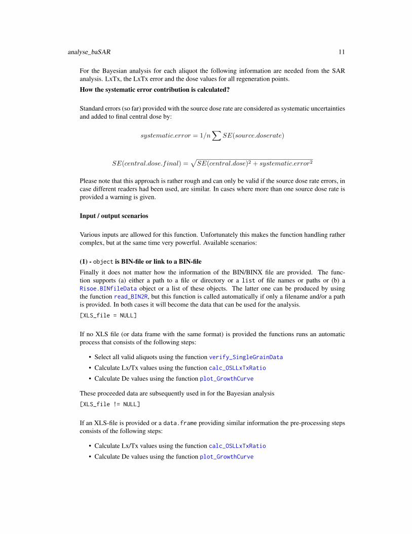
For the Bayesian analysis for each aliquot the following information are needed from the SARanalysis. LxTx, the LxTx error and the dose values for all regeneration points.

How the systematic error contribution is calculated?

Standard errors (so far) provided with the source dose rate are considered as systematic uncertaintiesand added to final central dose by:

systematic.error = 1/n∑

SE(source.doserate)

SE(central.dose.final) =√SE(central.dose)2 + systematic.error2

Please note that this approach is rather rough and can only be valid if the source dose rate errors, incase different readers had been used, are similar. In cases where more than one source dose rate isprovided a warning is given.

Input / output scenarios

Various inputs are allowed for this function. Unfortunately this makes the function handling rathercomplex, but at the same time very powerful. Available scenarios:

(1) - object is BIN-file or link to a BIN-fileFinally it does not matter how the information of the BIN/BINX file are provided. The func-tion supports (a) either a path to a file or directory or a list of file names or paths or (b) aRisoe.BINfileData object or a list of these objects. The latter one can be produced by usingthe function read_BIN2R, but this function is called automatically if only a filename and/or a pathis provided. In both cases it will become the data that can be used for the analysis.

[XLS_file = NULL]

If no XLS file (or data frame with the same format) is provided the functions runs an automaticprocess that consists of the following steps:

• Select all valid aliquots using the function verify_SingleGrainData

• Calculate Lx/Tx values using the function calc_OSLLxTxRatio

• Calculate De values using the function plot_GrowthCurve

These proceeded data are subsequently used in for the Bayesian analysis

[XLS_file != NULL]

If an XLS-file is provided or a data.frame providing similar information the pre-processing stepsconsists of the following steps:

• Calculate Lx/Tx values using the function calc_OSLLxTxRatio

• Calculate De values using the function plot_GrowthCurve

12 analyse_baSAR

Means, the XLS file should contain a selection of the BIN-file names and the aliquots selected forthe further analysis. This allows a manual selection of input data, as the automatic selection byverify_SingleGrainData might be not totally sufficient.

(2) - object RLum.Results object

If an RLum.Results object is provided as input and(!) this object was previously created by thefunction analyse_baSAR() itself, the pre-processing part is skipped and the function starts di-rectly the Bayesian analysis. This option is very powerful as it allows to change parameters for theBayesian analysis without the need to repeat the data pre-processing. If furthermore the argumentaliquot_range is set, aliquots can be manually excluded based on previous runs.

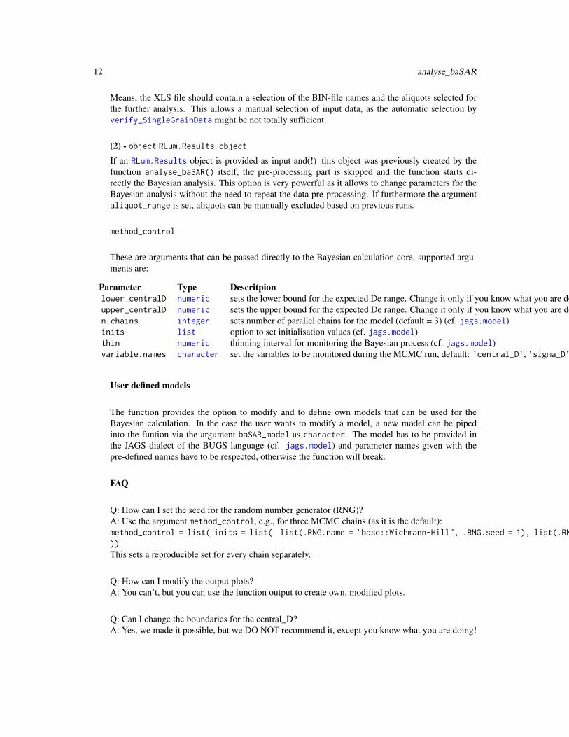
method_control

These are arguments that can be passed directly to the Bayesian calculation core, supported argu-ments are:

Parameter Type Descritpionlower_centralD numeric sets the lower bound for the expected De range. Change it only if you know what you are doing!upper_centralD numeric sets the upper bound for the expected De range. Change it only if you know what you are doing!n.chains integer sets number of parallel chains for the model (default = 3) (cf. jags.model)inits list option to set initialisation values (cf. jags.model)thin numeric thinning interval for monitoring the Bayesian process (cf. jags.model)variable.names character set the variables to be monitored during the MCMC run, default: ’central_D’, ’sigma_D’, ’D’, ’Q’, ’a’, ’b’, ’c’, ’g’. Note: only variables present in the model can be monitored.

User defined models

The function provides the option to modify and to define own models that can be used for theBayesian calculation. In the case the user wants to modify a model, a new model can be pipedinto the funtion via the argument baSAR_model as character. The model has to be provided inthe JAGS dialect of the BUGS language (cf. jags.model) and parameter names given with thepre-defined names have to be respected, otherwise the function will break.

FAQ

Q: How can I set the seed for the random number generator (RNG)?A: Use the argument method_control, e.g., for three MCMC chains (as it is the default):method_control = list( inits = list( list(.RNG.name = "base::Wichmann-Hill", .RNG.seed = 1), list(.RNG.name = "base::Wichmann-Hill", .RNG.seed = 2), list(.RNG.name = "base::Wichmann-Hill", .RNG.seed = 3)))This sets a reproducible set for every chain separately.

Q: How can I modify the output plots?A: You can’t, but you can use the function output to create own, modified plots.

Q: Can I change the boundaries for the central_D?A: Yes, we made it possible, but we DO NOT recommend it, except you know what you are doing!

analyse_baSAR 13

Example: method_control = list(lower_centralD = 10))

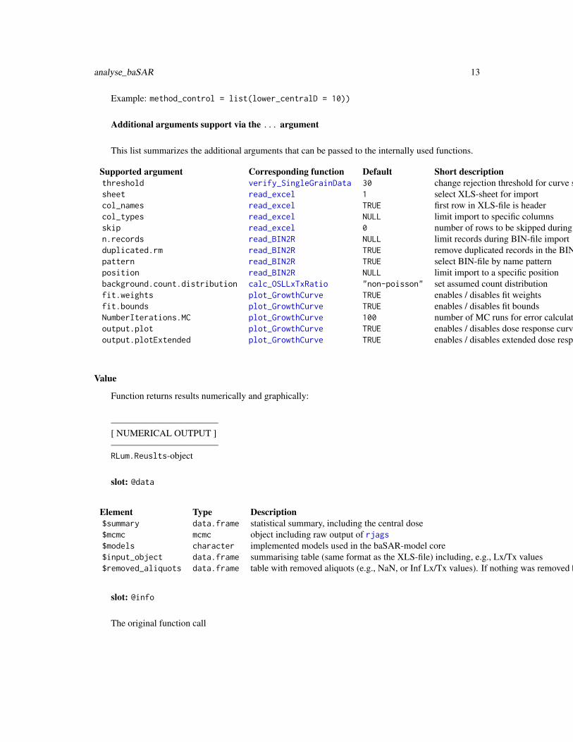
Additional arguments support via the ... argument

This list summarizes the additional arguments that can be passed to the internally used functions.

Supported argument Corresponding function Default Short descriptionthreshold verify_SingleGrainData 30 change rejection threshold for curve selectionsheet read_excel 1 select XLS-sheet for importcol_names read_excel TRUE first row in XLS-file is headercol_types read_excel NULL limit import to specific columnsskip read_excel 0 number of rows to be skipped during importn.records read_BIN2R NULL limit records during BIN-file importduplicated.rm read_BIN2R TRUE remove duplicated records in the BIN-filepattern read_BIN2R TRUE select BIN-file by name patternposition read_BIN2R NULL limit import to a specific positionbackground.count.distribution calc_OSLLxTxRatio "non-poisson" set assumed count distributionfit.weights plot_GrowthCurve TRUE enables / disables fit weightsfit.bounds plot_GrowthCurve TRUE enables / disables fit boundsNumberIterations.MC plot_GrowthCurve 100 number of MC runs for error calculationoutput.plot plot_GrowthCurve TRUE enables / disables dose response curve plotoutput.plotExtended plot_GrowthCurve TRUE enables / disables extended dose response curve plot

Value

Function returns results numerically and graphically:

———————————–[ NUMERICAL OUTPUT ]———————————–RLum.Reuslts-object

slot: @data

Element Type Description$summary data.frame statistical summary, including the central dose$mcmc mcmc object including raw output of rjags$models character implemented models used in the baSAR-model core$input_object data.frame summarising table (same format as the XLS-file) including, e.g., Lx/Tx values$removed_aliquots data.frame table with removed aliquots (e.g., NaN, or Inf Lx/Tx values). If nothing was removed NULL is returned

slot: @info

The original function call

14 analyse_baSAR

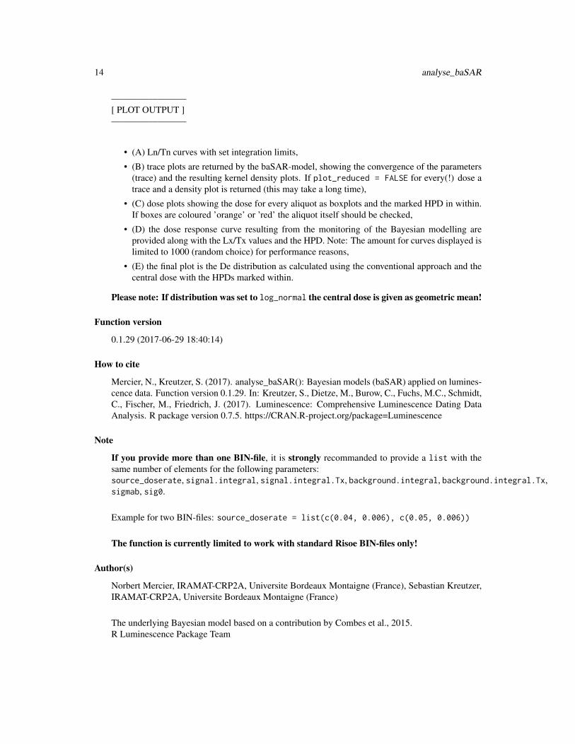
————————[ PLOT OUTPUT ]————————

• (A) Ln/Tn curves with set integration limits,

• (B) trace plots are returned by the baSAR-model, showing the convergence of the parameters(trace) and the resulting kernel density plots. If plot_reduced = FALSE for every(!) dose atrace and a density plot is returned (this may take a long time),

• (C) dose plots showing the dose for every aliquot as boxplots and the marked HPD in within.If boxes are coloured ’orange’ or ’red’ the aliquot itself should be checked,

• (D) the dose response curve resulting from the monitoring of the Bayesian modelling areprovided along with the Lx/Tx values and the HPD. Note: The amount for curves displayed islimited to 1000 (random choice) for performance reasons,

• (E) the final plot is the De distribution as calculated using the conventional approach and thecentral dose with the HPDs marked within.

Please note: If distribution was set to log_normal the central dose is given as geometric mean!

Function version

0.1.29 (2017-06-29 18:40:14)

How to cite

Mercier, N., Kreutzer, S. (2017). analyse_baSAR(): Bayesian models (baSAR) applied on lumines-cence data. Function version 0.1.29. In: Kreutzer, S., Dietze, M., Burow, C., Fuchs, M.C., Schmidt,C., Fischer, M., Friedrich, J. (2017). Luminescence: Comprehensive Luminescence Dating DataAnalysis. R package version 0.7.5. https://CRAN.R-project.org/package=Luminescence

Note

If you provide more than one BIN-file, it is strongly recommanded to provide a list with thesame number of elements for the following parameters:source_doserate, signal.integral, signal.integral.Tx, background.integral, background.integral.Tx,sigmab, sig0.

Example for two BIN-files: source_doserate = list(c(0.04, 0.006), c(0.05, 0.006))

The function is currently limited to work with standard Risoe BIN-files only!

Author(s)

Norbert Mercier, IRAMAT-CRP2A, Universite Bordeaux Montaigne (France), Sebastian Kreutzer,IRAMAT-CRP2A, Universite Bordeaux Montaigne (France)

The underlying Bayesian model based on a contribution by Combes et al., 2015.R Luminescence Package Team

analyse_baSAR 15

References

Combes, B., Philippe, A., Lanos, P., Mercier, N., Tribolo, C., Guerin, G., Guibert, P., Lahaye,C., 2015. A Bayesian central equivalent dose model for optically stimulated luminescence dating.Quaternary Geochronology 28, 62-70. doi:10.1016/j.quageo.2015.04.001

Mercier, N., Kreutzer, S., Christophe, C., Guerin, G., Guibert, P., Lahaye, C., Lanos, P., Philippe,A., Tribolo, C., 2016. Bayesian statistics in luminescence dating: The ’baSAR’-model and itsimplementation in the R package ’Luminescence’. Ancient TL 34, 14-21.

Further reading

Gelman, A., Carlin, J.B., Stern, H.S., Dunson, D.B., Vehtari, A., Rubin, D.B., 2013. Bayesian DataAnalysis, Third Edition. CRC Press.

Murray, A.S., Wintle, A.G., 2000. Luminescence dating of quartz using an improved single-aliquotregenerative-dose protocol. Radiation Measurements 32, 57-73. doi:10.1016/S1350-4487(99)00253-X

See Also

read_BIN2R, calc_OSLLxTxRatio, plot_GrowthCurve, read_excel, verify_SingleGrainData,jags.model, coda.samples, boxplot.default

Examples

##(1) load package test data setdata(ExampleData.BINfileData, envir = environment())

##(2) selecting relevant curves, and limit datasetCWOSL.SAR.Data <- subset(CWOSL.SAR.Data,subset = POSITION%in%c(1:3) & LTYPE == "OSL")

## Not run:##(3) run analysis##please not that the here selected parameters are##choosen for performance, not for reliabilityresults <- analyse_baSAR(object = CWOSL.SAR.Data,source_doserate = c(0.04, 0.001),signal.integral = c(1:2),background.integral = c(80:100),fit.method = "LIN",plot = FALSE,n.MCMC = 200

)

print(results)

##XLS_file template

16 analyse_FadingMeasurement

##copy and paste this the code below in the terminal##you can further use the function write.csv() to export the example

XLS_file <-structure(list(BIN_FILE = NA_character_,DISC = NA_real_,GRAIN = NA_real_),.Names = c("BIN_FILE", "DISC", "GRAIN"),class = "data.frame",row.names = 1L

)

## End(Not run)

analyse_FadingMeasurement

Analyse fading measurements and returns the fading rate per decade(g-value)

Description

The function analysis fading measurements and returns a fading rate including an error estimation.The function is not limited to standard fading measurements, as can be seen, e.g., Huntley andLamothe 2001. Additionally, the density of recombination centres (rho’) is estimated after Kars etal. 2008.

Usage

analyse_FadingMeasurement(object, structure = c("Lx", "Tx"), signal.integral,background.integral, t_star = "half", n.MC = 100, verbose = TRUE,plot = TRUE, plot.single = FALSE, ...)

Arguments

object RLum.Analysis (required): input object with the measurement data. Alterna-tively, a list containing RLum.Analysis objects or a data.frame with threecolumns (x = LxTx, y = LxTx error, z = time since irradiation) can be provided.Can also be a wide table, i.e. a data.frame with a number of colums divisibleby 3 and where each triplet has the before mentioned column structure.

structure character (with default): sets the structure of the measurement data. Allowedare 'Lx' or c('Lx','Tx'). Other input is ignored

signal.integral

vector (required): vector with the limits for the signal integral. Not requiredif a data.frame with LxTx values are provided.

analyse_FadingMeasurement 17

background.integral

vector (required): vector with the bounds for the background integral. Notrequired if a data.frame with LxTx values are provided.

t_star character (with default): method for calculating the time elasped since irradi-aton. Options are: 'half', which is tstar := t1 + (t2 − t1)/2 (Auclair et al.,2003) and 'end', which takes the time between irradiation and the measurementstep. Default is 'half'

n.MC integer (with default): number for Monte Carlo runs for the error estimation

verbose logical (with default): enables/disables verbose mode

plot logical (with default): enables/disables plot output

plot.single logical (with default): enables/disables single plot mode, i.e. one plot win-dow per plot. Alternatively a vector specifying the plot to be drawn, e.g.,plot.single = c(3,4) draws only the last two plots

... (optional) further arguments that can be passed to internally used functions (seedetails)

Details

All provided output corresponds to the tc value obtained by this analysis. Additionally in the outputobject the g-value normalised to 2-days is provided. The output of this function can be passed tothe function calc_FadingCorr.

Fitting and error estimation

For the fitting the function lm is used without applying weights. For the error estimation all inputvalues, except tc, as the precision can be consdiered as sufficiently high enough with regard to theunderlying problem, are sampled assuming a normal distribution for each value with the value asthe mean and the provided uncertainty as standard deviation.

Density of recombination centresThe density of recombination centres, expressed by the dimensionless variable rho’, is estimated byfitting equation 5 in Kars et al. 2008 to the data. For the fitting the function nls is used withoutapplying weights. For the error estimation the same procedure as for the g-value is applied (seeabove).

Value

An RLum.Results object is returned:

Slot: @data

OBJECT TYPE COMMENTfading_results data.frame results of the fading measurement in a tablefit lm object returned by the used linear fitting function lmrho_prime data.frame results of rho’ estimation after Kars et al. 2008LxTx_table data.frame Lx/Tx table, if curve data had been providedirr.times integer vector with the irradiation times in seconds

18 analyse_FadingMeasurement

Slot: @info

OBJECT TYPE COMMENTcall call the original function call

Function version

0.1.5 (2017-06-29 18:40:14)

How to cite

Kreutzer, S., Burow, C. (2017). analyse_FadingMeasurement(): Analyse fading measurementsand returns the fading rate per decade (g-value). Function version 0.1.5. In: Kreutzer, S., Di-etze, M., Burow, C., Fuchs, M.C., Schmidt, C., Fischer, M., Friedrich, J. (2017). Luminescence:Comprehensive Luminescence Dating Data Analysis. R package version 0.7.5. https://CRAN.R-project.org/package=Luminescence

Note

This function has BETA status and should not be used for publication work!

Author(s)

Sebastian Kreutzer, IRAMAT-CRP2A, Universite Bordeaux Montaigne (France)Christoph Burow, University of Cologne (Germany)R Luminescence Package Team

References

Auclair, M., Lamothe, M., Huot, S., 2003. Measurement of anomalous fading for feldpsar IRSLusing SAR. Radiation Measurements 37, 487-492. doi:10.1016/S1350-4487(03)00018-0

Huntley, D.J., Lamothe, M., 2001. Ubiquity of anomalous fading in K-feldspars and the measure-ment and correction for it in optical dating. Canadian Journal of Earth Sciences 38, 1093-1106.doi:10.1139/cjes-38-7-1093

Kars, R.H., Wallinga, J., Cohen, K.M., 2008. A new approach towards anomalous fading correctionfor feldspar IRSL dating-tests on samples in field saturation. Radiation Measurements 43, 786-790.doi:10.1016/j.radmeas.2008.01.021

See Also

calc_OSLLxTxRatio, read_BIN2R, read_XSYG2R, extract_IrradiationTimes

Examples

## load example data (sample UNIL/NB123, see ?ExampleData.Fading)data("ExampleData.Fading", envir = environment())

analyse_IRSAR.RF 19

##(1) get fading measurement data (here a three column data.frame)fading_data <- ExampleData.Fading$fading.data$IR50

##(2) run analysisg_value <- analyse_FadingMeasurement(fading_data,plot = TRUE,verbose = TRUE,n.MC = 10)

##(3) this can be further used in the function## to correct the age according to Huntley & Lamothe, 2001results <- calc_FadingCorr(age.faded = c(100,2),g_value = g_value,n.MC = 10)

analyse_IRSAR.RF Analyse IRSAR RF measurements

Description

Function to analyse IRSAR RF measurements on K-feldspar samples, performed using the protocolaccording to Erfurt et al. (2003) and beyond.

Usage

analyse_IRSAR.RF(object, sequence_structure = c("NATURAL", "REGENERATED"),RF_nat.lim = NULL, RF_reg.lim = NULL, method = "FIT",method.control = NULL, test_parameters = NULL, n.MC = 10,txtProgressBar = TRUE, plot = TRUE, plot_reduced = FALSE, ...)

Arguments

object RLum.Analysis or a list of RLum.Analysis objects (required): input objectcontaining data for protocol analysis. The function expects to find at least twocurves in the RLum.Analysis object: (1) RF_nat, (2) RF_reg. If a list is pro-vided as input all other parameters can be provided as list as well to gain fullcontrol.

sequence_structure

vector character (with default): specifies the general sequence structure. Al-lowed steps are NATURAL, REGENERATED. In addition any other character is al-lowed in the sequence structure; such curves will be ignored during the analysis.

RF_nat.lim vector (with default): set minimum and maximum channel range for naturalsignal fitting and sliding. If only one value is provided this will be treated asminimum value and the maximum limit will be added automatically.

20 analyse_IRSAR.RF

RF_reg.lim vector (with default): set minimum and maximum channel range for regener-ated signal fitting and sliding. If only one value is provided this will be treatedas minimum value and the maximum limit will be added automatically.

method character (with default): setting method applied for the data analysis. Possibleoptions are "FIT" or "SLIDE".

method.control list (optional): parameters to control the method, that can be passed to the cho-sen method. These are for (1) method = "FIT": ’trace’, ’maxiter’, ’warnOnly’,’minFactor’ and for (2) method = "SLIDE": ’correct_onset’, ’show_density’,’show_fit’, ’trace’. See details.

test_parameters

list (with default): set test parameters. Supported parameters are: curves_ratio,residuals_slope (only for method = "SLIDE"), curves_bounds, dynamic_ratio,lambda, beta and delta.phi. All input: numeric values, NA and NULL (s. De-tails)(see Details for further information)

n.MC numeric (with default): set number of Monte Carlo runs for start parameter esti-mation (method = "FIT") or error estimation (method = "SLIDE"). This valuecan be set to NULL to skip the MC runs. Note: Large values will significantlyincrease the computation time

txtProgressBar logical (with default): enables TRUE or disables FALSE the progression barduring MC runs

plot logical (with default): plot output (TRUE or FALSE)

plot_reduced logical (optional): provides a reduced plot output if enabled to allow com-mon R plot combinations, e.g., par(mfrow(...)). If TRUE no residual plot isreturned; it has no effect if plot = FALSE

... further arguments that will be passed to the plot output. Currently supported ar-guments are main, xlab, ylab, xlim, ylim, log, legend (TRUE/FALSE), legend.pos,legend.text (passes argument to x,y in legend), xaxt

Details

The function performs an IRSAR analysis described for K-feldspar samples by Erfurt et al. (2003)assuming a negligible sensitivity change of the RF signal.

General Sequence Structure (according to Erfurt et al. (2003))

1. Measuring IR-RF intensity of the natural dose for a few seconds (RFnat)

2. Bleach the samples under solar conditions for at least 30 min without changing the geometry

3. Waiting for at least one hour

4. Regeneration of the IR-RF signal to at least the natural level (measuring (RFreg)

5. Fitting data with a stretched exponential function

6. Calculate the the palaeodose De using the parameters from the fitting

Actually two methods are supported to obtain the De: method = "FIT" and method = "SLIDE":

analyse_IRSAR.RF 21

method = "FIT"

The principle is described above and follows the original suggestions by Erfurt et al., 2003. For thefitting the mean count value of the RF_nat curve is used.

Function used for the fitting (according to Erfurt et al. (2003)):

φ(D) = φ0 −∆φ(1− exp(−λ ∗D))β

with φ(D) the dose dependent IR-RF flux, φ0 the initial IR-RF flux, ∆φ the dose dependent changeof the IR-RF flux, λ the exponential parameter, D the dose and β the dispersive factor.

To obtain the palaeodose De the function is changed to:

De = ln(−(φ(D)− φ0)/(−λ ∗ φ)1/β + 1)/− λ

The fitting is done using the port algorithm of the nls function.

method = "SLIDE"

For this method the natural curve is slided along the x-axis until congruence with the regeneratedcurve is reached. Instead of fitting this allows to work with the original data without the need of anyphysical model. This approach was introduced for RF curves by Buylaert et al., 2012 and Lapp etal., 2012.

Here the sliding is done by searching for the minimum of the squared residuals. For the mathemat-ical details of the implementation see Frouin et al., 2017

method.control

To keep the generic argument list as clear as possible, arguments to control the methods for Deestimation are all preset with meaningful default parameters and can be handled using the argumentmethod.control only, e.g., method.control = list(trace = TRUE). Supported arguments are:

ARGUMENT METHOD DESCRIPTIONtrace FIT, SLIDE as in nls; shows sum of squared residualstrace_vslide SLIDE logical argument to enable or disable the tracing of the vertical slidingmaxiter FIT as in nlswarnOnly FIT as in nlsminFactor FIT as in nlscorrect_onset SLIDE The logical argument shifts the curves along the x-axis by the first channel, as light is expected in the first channel. The default value is TRUE.show_density SLIDE logical (with default) enables or disables KDE plots for MC run results. If the distribution is too narrow nothing is shown.show_fit SLIDE logical (with default) enables or disables the plot of the fitted curve routinely obtained during the evaluation.n.MC SLIDE integer (with default): This controls the number of MC runs within the sliding (assessing the possible minimum values). The default n.MC = 1000. Note: This parameter is not the same as controlled by the function argument n.MC.vslide_range SLDE logical or numeric or character (with default): This argument sets the boundaries for a vertical curve sliding. The argument expects a vector with an absolute minimum and a maximum (e.g., c(-1000,1000)). Alternatively the values NULL and ’auto’ are allowed. The automatic mode detects the reasonable vertical sliding range (recommended). NULL applies no vertical sliding. The default is NULL.cores SLIDE number or character (with default): set number of cores to be allocated for a parallel processing of the Monte-Carlo runs. The default value is NULL (single thread), the recommended values is ’auto’. An optional number (e.g., cores = 8) assigns a value manually.

22 analyse_IRSAR.RF

Error estimation

For method = "FIT" the asymmetric error range is obtained by using the 2.5 % (lower) and the97.5 % (upper) quantiles of the RFnat curve for calculating the De error range.

For method = "SLIDE" the error is obtained by bootstrapping the residuals of the slided curve toconstruct new natural curves for a Monte Carlo simulation. The error is returned in two ways: (a)the standard deviation of the herewith obtainedDe from the MC runs and (b) the confidence intervalusing the 2.5 % (lower) and the 97.5 % (upper) quantiles. The results of the MC runs are returnedwith the function output.

Test parameters

The argument test_parameters allows to pass some thresholds for several test parameters, whichwill be evaluated during the function run. If a threshold is set and it will be exceeded the testparameter status will be set to "FAILED". Intentionally this parameter is not termed ’rejectioncriteria’ as not all test parameters are evaluated for both methods and some parameters are calculatedby not evaluated by default. Common for all parameters are the allowed argument options NA andNULL. If the parameter is set to NA the value is calculated but the result will not be evaluated, meansit has no effect on the status ("OK" or "FAILED") of the parameter. Setting the parameter toNULL disables the parameter entirely and the parameter will be also removed from the functionoutput. This might be useful in cases where a particular parameter asks for long computation times.Currently supported parameters are:

curves_ratio numeric (default: 1.001):

The ratio of RFnat over RFreg in the range ofRFnat of is calculated and should not exceed thethreshold value.

intersection_ratio numeric (default: NA):

Calculated as absolute difference from 1 of the ratio of the integral of the normalised RF-curves,This value indicates intersection of the RF-curves and should be close to 0 if the curves have a sim-ilar shape. For this calculation first the corresponding time-count pair value on the RF_reg curve isobtained using the maximum count value of the RF_nat curve and only this segment (fitting to theRF_nat curve) on the RF_reg curve is taken for further calculating this ratio. If nothing is found atall, Inf is returned.

residuals_slope numeric (default: NA; only for method = "SLIDE"):

A linear function is fitted on the residuals after sliding. The corresponding slope can be used todiscard values as a high (positive, negative) slope may indicate that both curves are fundamentallydifferent and the method cannot be applied at all. Per default the value of this parameter is calcu-lated but not evaluated.

curves_bounds numeric (default: max(RFregcounts):

analyse_IRSAR.RF 23

This measure uses the maximum time (x) value of the regenerated curve. The maximum time (x)value of the natural curve cannot be larger than this value. However, although this is not recom-mended the value can be changed or disabled.

dynamic_ratio numeric (default: NA):

The dynamic ratio of the regenerated curve is calculated as ratio of the minimum and maximumcount values.

lambda, beta and delta.phi numeric (default: NA; method = "SLIDE"):

The stretched exponential function suggested by Erfurt et al. (2003) describing the decay of theRF signal, comprises several parameters that might be useful to evaluate the shape of the curves.For method = "FIT" this parameter is obtained during the fitting, for method = "SLIDE" a ratherrough estimation is made using the function nlsLM and the equation given above. Note: As thisprocedure requests more computation time, setting of one of these three parameters to NULL alsoprevents a calculation of the remaining two.

Value

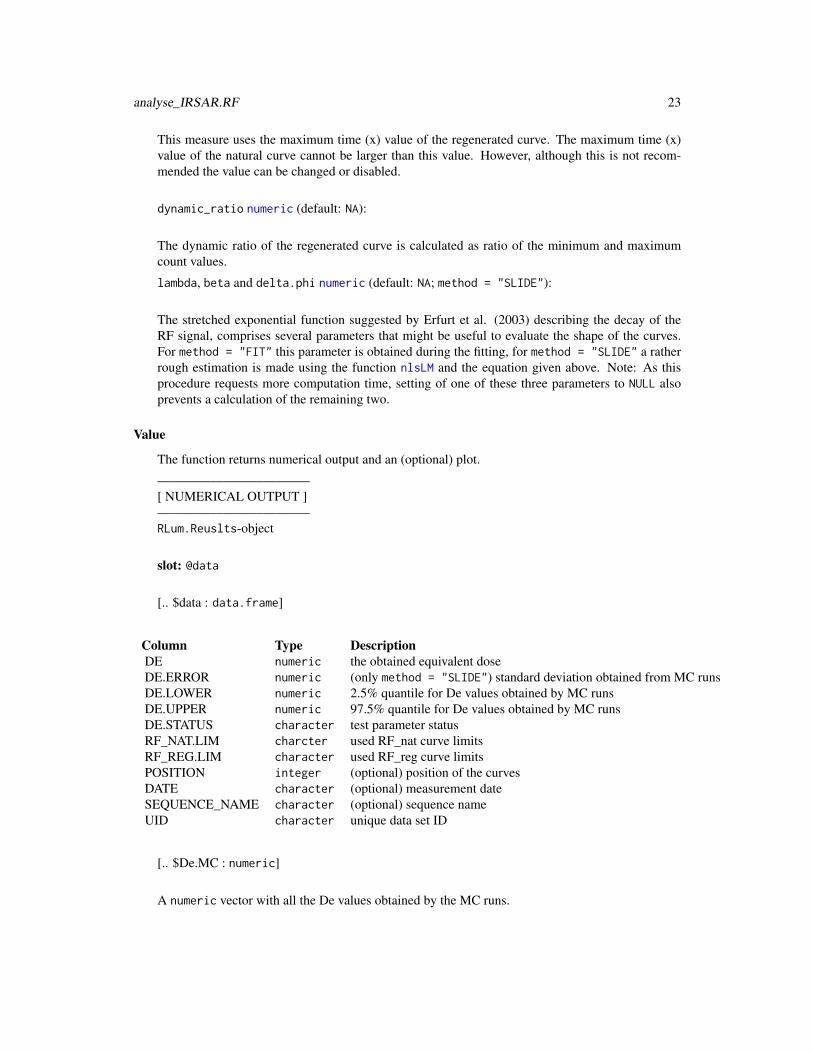
The function returns numerical output and an (optional) plot.


slot: @data

[.. $data : data.frame]

Column Type DescriptionDE numeric the obtained equivalent doseDE.ERROR numeric (only method = "SLIDE") standard deviation obtained from MC runsDE.LOWER numeric 2.5% quantile for De values obtained by MC runsDE.UPPER numeric 97.5% quantile for De values obtained by MC runsDE.STATUS character test parameter statusRF_NAT.LIM charcter used RF_nat curve limitsRF_REG.LIM character used RF_reg curve limitsPOSITION integer (optional) position of the curvesDATE character (optional) measurement dateSEQUENCE_NAME character (optional) sequence nameUID character unique data set ID

[.. $De.MC : numeric]

A numeric vector with all the De values obtained by the MC runs.

24 analyse_IRSAR.RF

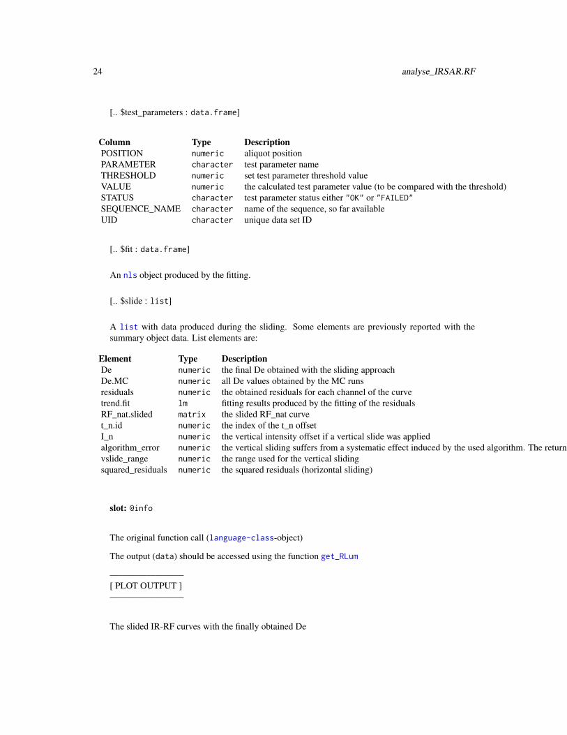
[.. $test_parameters : data.frame]

Column Type DescriptionPOSITION numeric aliquot positionPARAMETER character test parameter nameTHRESHOLD numeric set test parameter threshold valueVALUE numeric the calculated test parameter value (to be compared with the threshold)STATUS character test parameter status either "OK" or "FAILED"SEQUENCE_NAME character name of the sequence, so far availableUID character unique data set ID

[.. $fit : data.frame]

An nls object produced by the fitting.

[.. $slide : list]

A list with data produced during the sliding. Some elements are previously reported with thesummary object data. List elements are:

Element Type DescriptionDe numeric the final De obtained with the sliding approachDe.MC numeric all De values obtained by the MC runsresiduals numeric the obtained residuals for each channel of the curvetrend.fit lm fitting results produced by the fitting of the residualsRF_nat.slided matrix the slided RF_nat curvet_n.id numeric the index of the t_n offsetI_n numeric the vertical intensity offset if a vertical slide was appliedalgorithm_error numeric the vertical sliding suffers from a systematic effect induced by the used algorithm. The returned value is the standard deviation of all obtained De values while expanding the vertical sliding range. I can be added as systematic error to the final De error; so far wanted.vslide_range numeric the range used for the vertical slidingsquared_residuals numeric the squared residuals (horizontal sliding)

slot: @info

The original function call (language-class-object)

The output (data) should be accessed using the function get_RLum

————————[ PLOT OUTPUT ]————————

The slided IR-RF curves with the finally obtained De

analyse_IRSAR.RF 25

Function version

0.7.2 (2017-06-29 18:40:14)

How to cite

Kreutzer, S. (2017). analyse_IRSAR.RF(): Analyse IRSAR RF measurements. Function version0.7.2. In: Kreutzer, S., Dietze, M., Burow, C., Fuchs, M.C., Schmidt, C., Fischer, M., Friedrich, J.(2017). Luminescence: Comprehensive Luminescence Dating Data Analysis. R package version0.7.5. https://CRAN.R-project.org/package=Luminescence

Note

This function assumes that there is no sensitivity change during the measurements (natural vs. re-generated signal), which is in contrast to the findings by Buylaert et al. (2012). Furthermore:In course of ongoing research this function has been almost fully re-written, but further thought-ful tests are still pending! However, as a lot new package functionality was introduced with thechanges made for this function and to allow a part of such tests the re-newed code was made part ofthe current package.

Author(s)

Sebastian Kreutzer, IRAMAT-CRP2A, Universite Bordeaux Montaigne (France)R Luminescence Package Team

References

Buylaert, J.P., Jain, M., Murray, A.S., Thomsen, K.J., Lapp, T., 2012. IR-RF dating of sand-sized K-feldspar extracts: A test of accuracy. Radiation Measurements 44 (5-6), 560-565. doi:10.1016/j.radmeas.2012.06.021

Erfurt, G., Krbetschek, M.R., 2003. IRSAR - A single-aliquot regenerative-dose dating protocolapplied to the infrared radiofluorescence (IR-RF) of coarse- grain K-feldspar. Ancient TL 21, 35-42.

Erfurt, G., 2003. Infrared luminescence of Pb+ centres in potassium-rich feldspars. physica statussolidi (a) 200, 429-438.

Erfurt, G., Krbetschek, M.R., 2003. Studies on the physics of the infrared radioluminescence ofpotassium feldspar and on the methodology of its application to sediment dating. Radiation Mea-surements 37, 505-510.

Erfurt, G., Krbetschek, M.R., Bortolot, V.J., Preusser, F., 2003. A fully automated multi-spectralradioluminescence reading system for geochronometry and dosimetry. Nuclear Instruments andMethods in Physics Research Section B: Beam Interactions with Materials and Atoms 207, 487-499.

Frouin, M., Huot, S., Kreutzer, S., Lahaye, C., Lamothe, M., Philippe, A., Mercier, N., 2017. Animproved radiofluorescence single-aliquot regenerative dose protocol for K-feldspars. QuaternaryGeochronology 38, 13-24. doi:10.1016/j.quageo.2016.11.004

Lapp, T., Jain, M., Thomsen, K.J., Murray, A.S., Buylaert, J.P., 2012. New luminescence measure-ment facilities in retrospective dosimetry. Radiation Measurements 47, 803-808. doi:10.1016/j.radmeas.2012.02.006

26 analyse_pIRIRSequence

Trautmann, T., 2000. A study of radioluminescence kinetics of natural feldspar dosimeters: experi-ments and simulations. Journal of Physics D: Applied Physics 33, 2304-2310.

Trautmann, T., Krbetschek, M.R., Dietrich, A., Stolz, W., 1998. Investigations of feldspar radiolu-minescence: potential for a new dating technique. Radiation Measurements 29, 421-425.

Trautmann, T., Krbetschek, M.R., Dietrich, A., Stolz, W., 1999. Feldspar radioluminescence: a newdating method and its physical background. Journal of Luminescence 85, 45-58.

Trautmann, T., Krbetschek, M.R., Stolz, W., 2000. A systematic study of the radioluminescenceproperties of single feldspar grains. Radiation Measurements 32, 685-690.

See Also

RLum.Analysis, RLum.Results, get_RLum, nls, nlsLM, mclapply

Examples

##load datadata(ExampleData.RLum.Analysis, envir = environment())

##(1) perform analysis using the method 'FIT'results <- analyse_IRSAR.RF(object = IRSAR.RF.Data)

##show De results and test paramter resultsget_RLum(results, data.object = "data")get_RLum(results, data.object = "test_parameters")

##(2) perform analysis using the method 'SLIDE'results <- analyse_IRSAR.RF(object = IRSAR.RF.Data, method = "SLIDE", n.MC = 1)

## Not run:##(3) perform analysis using the method 'SLIDE' and method control option## 'traceresults <- analyse_IRSAR.RF(object = IRSAR.RF.Data,method = "SLIDE",method.control = list(trace = TRUE))

## End(Not run)

analyse_pIRIRSequence Analyse post-IR IRSL sequences

Description

The function performs an analysis of post-IR IRSL sequences including curve fitting on RLum.Analysisobjects.

analyse_pIRIRSequence 27

Usage

analyse_pIRIRSequence(object, signal.integral.min, signal.integral.max,background.integral.min, background.integral.max, dose.points = NULL,sequence.structure = c("TL", "IR50", "pIRIR225"), plot = TRUE,plot.single = FALSE, ...)

Arguments

object RLum.Analysis (required) or list of RLum.Analysis objects: input objectcontaining data for analysis. If a list is provided the functions tries to iteratreover the list.

signal.integral.min

integer (required): lower bound of the signal integral. Provide this value asvector for different integration limits for the different IRSL curves.

signal.integral.max

integer (required): upper bound of the signal integral. Provide this value asvector for different integration limits for the different IRSL curves.

background.integral.min

integer (required): lower bound of the background integral. Provide this valueas vector for different integration limits for the different IRSL curves.

background.integral.max

integer (required): upper bound of the background integral. Provide this valueas vector for different integration limits for the different IRSL curves.

dose.points numeric (optional): a numeric vector containing the dose points values. Usingthis argument overwrites dose point values in the signal curves.

sequence.structure

vector character (with default): specifies the general sequence structure. Al-lowed values are "TL" and any "IR" combination (e.g., "IR50","pIRIR225").Additionally a parameter "EXCLUDE" is allowed to exclude curves from the anal-ysis (Note: If a preheat without PMT measurement is used, i.e. preheat as nonTL, remove the TL step.)

plot logical (with default): enables or disables plot output.

plot.single logical (with default): single plot output (TRUE/FALSE) to allow for plottingthe results in single plot windows. Requires plot = TRUE.

... further arguments that will be passed to the function analyse_SAR.CWOSL andplot_GrowthCurve

Details

To allow post-IR IRSL protocol (Thomsen et al., 2008) measurement analyses this function hasbeen written as extended wrapper function for the function analyse_SAR.CWOSL, facilitating an en-tire sequence analysis in one run. With this, its functionality is strictly limited by the functionalityof the function analyse_SAR.CWOSL.

If the input is a list

28 analyse_pIRIRSequence

If the input is a list of RLum.Analysis-objects, every argument can be provided as list to al-low for different sets of parameters for every single input element. For further information seeanalyse_SAR.CWOSL.

Value

Plots (optional) and an RLum.Results object is returned containing the following elements:

DATA.OBJECT TYPE DESCRIPTION..$data : data.frame Table with De values..$LnLxTnTx.table : data.frame with the LnLxTnTx values..$rejection.criteria : data.frame rejection criteria..$Formula : list Function used for fitting of the dose response curve..$call : call the original function call

The output should be accessed using the function get_RLum.

Function version

0.2.2 (2017-06-29 18:40:14)

How to cite

Kreutzer, S. (2017). analyse_pIRIRSequence(): Analyse post-IR IRSL sequences. Function version0.2.2. In: Kreutzer, S., Dietze, M., Burow, C., Fuchs, M.C., Schmidt, C., Fischer, M., Friedrich, J.(2017). Luminescence: Comprehensive Luminescence Dating Data Analysis. R package version0.7.5. https://CRAN.R-project.org/package=Luminescence

Note

Best graphical output can be achieved by using the function pdf with the following options:pdf(file = "...", height = 15, width = 15)

Author(s)


References

Murray, A.S., Wintle, A.G., 2000. Luminescence dating of quartz using an improved single-aliquotregenerative-dose protocol. Radiation Measurements 32, 57-73. doi:10.1016/S1350-4487(99)00253-X

Thomsen, K.J., Murray, A.S., Jain, M., Boetter-Jensen, L., 2008. Laboratory fading rates of vari-ous luminescence signals from feldspar-rich sediment extracts. Radiation Measurements 43, 1474-1486. doi:10.1016/j.radmeas.2008.06.002

analyse_pIRIRSequence 29

See Also

analyse_SAR.CWOSL, calc_OSLLxTxRatio, plot_GrowthCurve, RLum.Analysis, RLum.Resultsget_RLum

Examples

### NOTE: For this example existing example data are used. These data are non pIRIR data.#####(1) Compile example data set based on existing example data (SAR quartz measurement)##(a) Load example datadata(ExampleData.BINfileData, envir = environment())

##(b) Transform the values from the first position in a RLum.Analysis objectobject <- Risoe.BINfileData2RLum.Analysis(CWOSL.SAR.Data, pos=1)

##(c) Grep curves and exclude the last two (one TL and one IRSL)object <- get_RLum(object, record.id = c(-29,-30))

##(d) Define new sequence structure and set new RLum.Analysis objectsequence.structure <- c(1,2,2,3,4,4)sequence.structure <- as.vector(sapply(seq(0,length(object)-1,by = 4),

function(x){sequence.structure + x}))

object <- sapply(1:length(sequence.structure), function(x){

object[[sequence.structure[x]]]

})

object <- set_RLum(class = "RLum.Analysis", records = object, protocol = "pIRIR")

##(2) Perform pIRIR analysis (for this example with quartz OSL data!)## Note: output as single plots to avoid problems with this exampleresults <- analyse_pIRIRSequence(object,

signal.integral.min = 1,signal.integral.max = 2,background.integral.min = 900,background.integral.max = 1000,fit.method = "EXP",sequence.structure = c("TL", "pseudoIRSL1", "pseudoIRSL2"),main = "Pseudo pIRIR data set based on quartz OSL",plot.single = TRUE)

##(3) Perform pIRIR analysis (for this example with quartz OSL data!)## Alternative for PDF output, uncomment and complete for usage## Not run:pdf(file = "...", height = 15, width = 15)

results <- analyse_pIRIRSequence(object,signal.integral.min = 1,

30 analyse_portableOSL

signal.integral.max = 2,background.integral.min = 900,background.integral.max = 1000,fit.method = "EXP",main = "Pseudo pIRIR data set based on quartz OSL")

dev.off()

## End(Not run)

analyse_portableOSL Analyse portable CW-OSL measurements

Description

The function analyses CW-OSL curve data produced by a SUERC portable OSL reader and pro-duces a combined plot of OSL/IRSL signal intensities, OSL/IRSL depletion ratios and the IRSL/OSLratio.

Usage

analyse_portableOSL(object, signal.integral, invert = FALSE,normalise = FALSE, plot = TRUE, ...)

Arguments

object RLum.Analysis (required): RLum.Analysis object produced by read_PSL2R.signal.integral

vector (required): A vector of two values specifying the lower and upper chan-nel used to calculate the OSL/IRSL signal. Can be provided in form of c(1, 5)or 1:5.

invert logical (with default): TRUE to calculate and plot the data in reverse order.

normalise logical (with default): TRUE to normalise the OSL/IRSL signals by the meanof all corresponding data curves.

plot logical (with default): enable/disable plot output

... currently not used.

Details

This function only works with RLum.Analysis objects produced by read_PSL2R. It further assumes(or rather requires) an equal amount of OSL and IRSL curves that are pairwise combined for cal-culating the IRSL/OSL ratio. For calculating the depletion ratios the cumulative signal of the lastn channels (same number of channels as specified by signal.integral) is divided by cumulativesignal of the first n channels (signal.integral).

analyse_SAR.CWOSL 31

Value

Returns an S4 RLum.Results object containing the following elements:

Function version

0.0.3 (2017-06-29 18:40:14)

How to cite

Burow, C. (2017). analyse_portableOSL(): Analyse portable CW-OSL measurements. Functionversion 0.0.3. In: Kreutzer, S., Dietze, M., Burow, C., Fuchs, M.C., Schmidt, C., Fischer, M.,Friedrich, J. (2017). Luminescence: Comprehensive Luminescence Dating Data Analysis. R pack-age version 0.7.5. https://CRAN.R-project.org/package=Luminescence

Author(s)

Christoph Burow, University of Cologne (Germany)R Luminescence Package Team

See Also

RLum.Analysis, RLum.Data.Curve

Examples

# (1) load example data setdata("ExampleData.portableOSL", envir = environment())

# (2) merge and plot all RLum.Analysis objectsmerged <- merge_RLum(ExampleData.portableOSL)plot_RLum(merged, combine = TRUE)merged

# (3) analyse and plotresults <- analyse_portableOSL(merged, signal.integral = 1:5, invert = FALSE, normalise = TRUE)get_RLum(results)

analyse_SAR.CWOSL Analyse SAR CW-OSL measurements

Description

The function performs a SAR CW-OSL analysis on an RLum.Analysis object including growthcurve fitting.

32 analyse_SAR.CWOSL

Usage

analyse_SAR.CWOSL(object, signal.integral.min, signal.integral.max,background.integral.min, background.integral.max, rejection.criteria = NULL,dose.points = NULL, mtext.outer, plot = TRUE, plot.single = FALSE, ...)

Arguments

object RLum.Analysis (required): input object containing data for analysis, alterna-tively a list of RLum.Analysis objects can be provided.

signal.integral.min

integer (required): lower bound of the signal integral. Can be a list ofintegers, if object is of type list. If the input is vector (e.g., c(1,2)) the2nd value will be interpreted as the minimum signal integral for the Tx curve.

signal.integral.max

integer (required): upper bound of the signal integral. Can be a list ofintegers, if object is of type list. If the input is vector (e.g., c(1,2)) the2nd value will be interpreted as the maximum signal integral for the Tx curve.

background.integral.min

integer (required): lower bound of the background integral. Can be a list ofintegers, if object is of type list. If the input is vector (e.g., c(1,2)) the 2ndvalue will be interpreted as the minimum background integral for the Tx curve.

background.integral.max

integer (required): upper bound of the background integral. Can be a listof integers, if object is of type list. If the input is vector (e.g., c(1,2)) the2nd value will be interpreted as the maximum background integral for the Txcurve.

rejection.criteria

list (with default): provide a named list and set rejection criteria in percentagefor further calculation. Can be a list in a list, if object is of type list

Allowed arguments are recycling.ratio, recuperation.rate, palaeodose.error,testdose.error and exceed.max.regpoint = TRUE/FALSE. Example: rejection.criteria = list(recycling.ratio = 10).Per default all numerical values are set to 10, exceed.max.regpoint = TRUE.Every criterium can be set to NA. In this value are calculated, but not considered,i.e. the RC.Status becomes always 'OK'

dose.points numeric (optional): a numeric vector containg the dose points values Using thisargument overwrites dose point values in the signal curves. Can be a list ofnumeric vectors, if object is of type list

mtext.outer character (optional): option to provide an outer margin mtext. Can be a listof characters, if object is of type list

plot logical (with default): enables or disables plot output.

plot.single logical (with default) or numeric (optional): single plot output (TRUE/FALSE)to allow for plotting the results in single plot windows. If a numerice vec-tor is provided the plots can be selected individually, i.e. plot.single =c(1,2,3,4) will plot the TL and Lx, Tx curves but not the legend (5) or thegrowth curve (6), (7) and (8) belong to rejection criteria plots. Requires plot = TRUE.


... further arguments that will be passed to the function plot_GrowthCurve orcalc_OSLLxTxRatio (supported: background.count.distribution, sigmab,sig0). Please note that if you consider to use the early light subtraction methodyou should provide your own sigmab value!

Details

The function performs an analysis for a standard SAR protocol measurements introduced by Mur-ray and Wintle (2000) with CW-OSL curves. For the calculation of the Lx/Tx value the func-tion calc_OSLLxTxRatio is used. For changing the way the Lx/Tx error is calculated use theargument background.count.distribution and sigmab, which will be passed to the functioncalc_OSLLxTxRatio.

Argument object is of type list

If the argument object is of type list containing only RLum.Analysis objects, the function re-calls itself as often as elements are in the list. This is usefull if an entire measurement wantedto be analysed without writing separate for-loops. To gain in full control of the parameters (e.g.,dose.points) for every aliquot (corresponding to one RLum.Analysis object in the list), in thiscase the arguments can be provided as list. This list should be of similar length as the listprovided with the argument object, otherwise the function will create an own list of the requestedlenght. Function output will be just one single RLum.Results object.

Please be careful when using this option. It may allow a fast an efficient data analysis, but thefunction may also break with an unclear error message, due to wrong input data.

Working with IRSL data

The function was originally designed to work just for ’OSL’ curves, following the principles of theSAR protocol. An IRSL measurement protocol may follow this procedure, e.g., post-IR IRSL pro-tocol (Thomsen et al., 2008). Therefore this functions has been enhanced to work with IRSL data,however, the function is only capable of analysing curves that follow the SAR protocol structure,i.e., to analyse a post-IR IRSL protocol, curve data have to be pre-selected by the user to fit thestandards of the SAR protocol, i.e., Lx,Tx,Lx,Tx and so on.

Example: Imagine the measurement contains pIRIR50 and pIRIR225 IRSL curves. Only one curvetype can be analysed at the same time: The pIRIR50 curves or the pIRIR225 curves.

Supported rejection criteria

‘recycling.ratio’: calculated for every repeated regeneration dose point.

34 analyse_SAR.CWOSL

‘recuperation.rate’: recuperation rate calculated by comparing the Lx/Tx values of the zero regen-eration point with the Ln/Tn value (the Lx/Tx ratio of the natural signal). For methodologicalbackground see Aitken and Smith (1988).

‘testdose.error’: set the allowed error for the testdose, which per default should not exceed 10%.The testdose error is calculated as Tx_net.error/Tx_net.

‘palaeodose.error’: set the allowed error for the De value, which per default should not exceed 10%.

Value

A plot (optional) and an RLum.Results object is returned containing the following elements:

data data.frame containing De-values, De-error and further parametersLnLxTnTx.values

data.frame of all calculated Lx/Tx values including signal, background countsand the dose points

rejection.criteria

data.frame with values that might by used as rejection criteria. NA is producedif no R0 dose point exists.

Formula formula formula that have been used for the growth curve fitting


Function version

0.7.10 (2017-06-29 18:40:14)

How to cite

Kreutzer, S. (2017). analyse_SAR.CWOSL(): Analyse SAR CW-OSL measurements. Functionversion 0.7.10. In: Kreutzer, S., Dietze, M., Burow, C., Fuchs, M.C., Schmidt, C., Fischer, M.,Friedrich, J. (2017). Luminescence: Comprehensive Luminescence Dating Data Analysis. R pack-age version 0.7.5. https://CRAN.R-project.org/package=Luminescence

Note

This function must not be mixed up with the function Analyse_SAR.OSLdata, which works withRisoe.BINfileData-class objects.

The function currently does only support ’OSL’ or ’IRSL’ data!

Author(s)



References

Aitken, M.J. and Smith, B.W., 1988. Optical dating: recuperation after bleaching. QuaternaryScience Reviews 7, 387-393.

Duller, G., 2003. Distinguishing quartz and feldspar in single grain luminescence measurements.Radiation Measurements, 37 (2), 161-165.

Murray, A.S. and Wintle, A.G., 2000. Luminescence dating of quartz using an improved single-aliquot regenerative-dose protocol. Radiation Measurements 32, 57-73.

Thomsen, K.J., Murray, A.S., Jain, M., Boetter-Jensen, L., 2008. Laboratory fading rates of vari-ous luminescence signals from feldspar-rich sediment extracts. Radiation Measurements 43, 1474-1486. doi:10.1016/j.radmeas.2008.06.002

See Also

calc_OSLLxTxRatio, plot_GrowthCurve, RLum.Analysis, RLum.Results get_RLum

Examples

##load data##ExampleData.BINfileData contains two BINfileData objects##CWOSL.SAR.Data and TL.SAR.Datadata(ExampleData.BINfileData, envir = environment())

##transform the values from the first position in a RLum.Analysis objectobject <- Risoe.BINfileData2RLum.Analysis(CWOSL.SAR.Data, pos=1)

##perform SAR analysis and set rejection criteriaresults <- analyse_SAR.CWOSL(object = object,signal.integral.min = 1,signal.integral.max = 2,background.integral.min = 900,background.integral.max = 1000,log = "x",fit.method = "EXP",rejection.criteria = list(

recycling.ratio = 10,recuperation.rate = 10,testdose.error = 10,palaeodose.error = 10,exceed.max.regpoint = TRUE)

)

##show De resultsget_RLum(results)

##show LnTnLxTx tableget_RLum(results, data.object = "LnLxTnTx.table")

36 Analyse_SAR.OSLdata

Analyse_SAR.OSLdata Analyse SAR CW-OSL measurements.

Description

The function analyses SAR CW-OSL curve data and provides a summary of the measured data forevery position. The output of the function is optimised for SAR OSL measurements on quartz.

Usage

Analyse_SAR.OSLdata(input.data, signal.integral, background.integral, position,run, set, dtype, keep.SEL = FALSE,info.measurement = "unkown measurement", output.plot = FALSE,output.plot.single = FALSE, cex.global = 1, ...)

Arguments

input.data Risoe.BINfileData-class (required): input data from a Risoe BIN file, producedby the function read_BIN2R.

signal.integral

vector (required): channels used for the signal integral, e.g. signal.integral=c(1:2)background.integral

vector (required): channels used for the background integral, e.g. background.integral=c(85:100)

position vector (optional): reader positions that want to be analysed (e.g. position=c(1:48).Empty positions are automatically omitted. If no value is given all positions areanalysed by default.

run vector (optional): range of runs used for the analysis. If no value is given therange of the runs in the sequence is deduced from the Risoe.BINfileData object.

set vector (optional): range of sets used for the analysis. If no value is given therange of the sets in the sequence is deduced from the Risoe.BINfileData ob-ject.

dtype character (optional): allows to further limit the curves by their data type(DTYPE), e.g., dtype = c("Natural","Dose") limits the curves to this twodata types. By default all values are allowed. See Risoe.BINfileData-class forallowed data types.

keep.SEL logical (default): option allowing to use the SEL element of the Risoe.BINfileData-class manually. NOTE: In this case any limitation provided by run, set anddtype are ignored!

info.measurement

character (with default): option to provide information about the measurementon the plot output (e.g. name of the BIN or BINX file).

output.plot logical (with default): plot output (TRUE/FALSE)output.plot.single

logical (with default): single plot output (TRUE/FALSE) to allow for plotting theresults in single plot windows. Requires output.plot = TRUE.

Analyse_SAR.OSLdata 37

cex.global numeric (with default): global scaling factor.

... further arguments that will be passed to the function calc_OSLLxTxRatio (sup-ported: background.count.distribution, sigmab, sig0; e.g., for instrumen-tal error) and can be used to adjust the plot. Supported" mtext, log

Details

The function works only for standard SAR protocol measurements introduced by Murray and Win-tle (2000) with CW-OSL curves. For the calculation of the Lx/Tx value the function calc_OSLLxTxRatiois used.

Provided rejection criteria

‘recyling ratio’: calculated for every repeated regeneration dose point.‘recuperation’: recuperation rate calculated by comparing the Lx/Tx values of the zero regenerationpoint with the Ln/Tn value (the Lx/Tx ratio of the natural signal). For methodological backgroundsee Aitken and Smith (1988)

‘IRSL/BOSL’: the integrated counts (signal.integral) of an IRSL curve are compared to theintegrated counts of the first regenerated dose point. It is assumed that IRSL curves got the samedose as the first regenerated dose point. Note: This is not the IR depletation ratio described byDuller (2003).

Value

A plot (optional) and list is returned containing the following elements:

LnLxTnTx data.frame of all calculated Lx/Tx values including signal, background countsand the dose points.

RejectionCriteria


SARParameters data.frame of additional measurement parameters obtained from the BIN file,e.g. preheat or read temperature (not valid for all types of measurements).

Function version

0.2.17 (2017-06-29 18:40:14)

How to cite

Kreutzer, S., Fuchs, M.C., Fuchs, M. (2017). Analyse_SAR.OSLdata(): Analyse SAR CW-OSLmeasurements.. Function version 0.2.17. In: Kreutzer, S., Dietze, M., Burow, C., Fuchs, M.C.,Schmidt, C., Fischer, M., Friedrich, J. (2017). Luminescence: Comprehensive Luminescence Dat-ing Data Analysis. R package version 0.7.5. https://CRAN.R-project.org/package=Luminescence

38 Analyse_SAR.OSLdata

Note

Rejection criteria are calculated but not considered during the analysis to discard values.

The analysis of IRSL data is not directly supported. You may want to consider using the func-tions analyse_SAR.CWOSL or analyse_pIRIRSequence instead.

The development of this function will not be continued. We recommend to use the functionanalyse_SAR.CWOSL or instead.

Author(s)

Sebastian Kreutzer, IRAMAT-CRP2A, Universite Bordeaux Montaigne (France), Margret C. Fuchs,HZDR, Freiberg (Germany)R Luminescence Package Team

References


Duller, G., 2003. Distinguishing quartz and feldspar in single grain luminescence measurements.Radiation Measurements, 37 (2), 161-165.


See Also

calc_OSLLxTxRatio, Risoe.BINfileData-class, read_BIN2R

and for further analysis plot_GrowthCurve

Examples

##load datadata(ExampleData.BINfileData, envir = environment())

##analyse dataoutput <- Analyse_SAR.OSLdata(input.data = CWOSL.SAR.Data,

signal.integral = c(1:5),background.integral = c(900:1000),position = c(1:1),output.plot = TRUE)

##combine results relevant for further analysisoutput.SAR <- data.frame(Dose = output$LnLxTnTx[[1]]$Dose,

LxTx = output$LnLxTnTx[[1]]$LxTx,LxTx.Error = output$LnLxTnTx[[1]]$LxTx.Error)

output.SAR

analyse_SAR.TL 39

analyse_SAR.TL Analyse SAR TL measurements

Description

The function performs a SAR TL analysis on a RLum.Analysis object including growth curvefitting.

Usage

analyse_SAR.TL(object, object.background, signal.integral.min,signal.integral.max, integral_input = "channel",sequence.structure = c("PREHEAT", "SIGNAL", "BACKGROUND"),rejection.criteria = list(recycling.ratio = 10, recuperation.rate = 10),dose.points, log = "", ...)

Arguments

object RLum.Analysis(required): input object containing data for analysisobject.background

currently not usedsignal.integral.min

integer (required): requires the channel number for the lower signal integralbound (e.g. signal.integral.min = 100)

signal.integral.max

integer (required): requires the channel number for the upper signal integralbound (e.g. signal.integral.max = 200)

integral_input character (with default): defines the input for the the arguments signal.integral.minand signal.integral.max. These limits can be either provided 'channel'number (the default) or 'temperature'. If 'temperature' is chosen the bestmatching channel is selected.

sequence.structure

vector character (with default): specifies the general sequence structure. Threesteps are allowed ( "PREHEAT", "SIGNAL", "BACKGROUND"), in addition a param-eter "EXCLUDE". This allows excluding TL curves which are not relevant for theprotocol analysis. (Note: None TL are removed by default)

rejection.criteria

list (with default): list containing rejection criteria in percentage for the calcula-tion.

dose.points numeric (optional): option set dose points manually

log character (with default): a character string which contains "x" if the x axis is tobe logarithmic, "y" if the y axis is to be logarithmic and "xy" or "yx" if both axesare to be logarithmic. See plot.default).

... further arguments that will be passed to the function plot_GrowthCurve

40 analyse_SAR.TL

Details

This function performs a SAR TL analysis on a set of curves. The SAR procedure in general is givenby Murray and Wintle (2000). For the calculation of the Lx/Tx value the function calc_TLLxTxRatiois used.

Provided rejection criteria

‘recyling.ratio’: calculated for every repeated regeneration dose point.‘recuperation.rate’: recuperation rate calculated by comparing the Lx/Tx values of the zero regen-eration point with the Ln/Tn value (the Lx/Tx ratio of the natural signal). For methodologicalbackground see Aitken and Smith (1988)

Value

A plot (optional) and an RLum.Results object is returned containing the following elements:

De.values data.frame containing De-values and further parametersLnLxTnTx.values

data.frame of all calculated Lx/Tx values including signal, background countsand the dose points.

rejection.criteria


note: the output should be accessed using the function get_RLum

Function version

0.2.0 (2017-06-29 18:40:14)

How to cite

Kreutzer, S. (2017). analyse_SAR.TL(): Analyse SAR TL measurements. Function version 0.2.0.In: Kreutzer, S., Dietze, M., Burow, C., Fuchs, M.C., Schmidt, C., Fischer, M., Friedrich, J. (2017).Luminescence: Comprehensive Luminescence Dating Data Analysis. R package version 0.7.5.https://CRAN.R-project.org/package=Luminescence

Note

THIS IS A BETA VERSION

None TL curves will be removed from the input object without further warning.

Author(s)


apply_CosmicRayRemoval 41

References



See Also

calc_TLLxTxRatio, plot_GrowthCurve, RLum.Analysis, RLum.Results get_RLum

Examples


##transform the values from the first position in a RLum.Analysis objectobject <- Risoe.BINfileData2RLum.Analysis(TL.SAR.Data, pos=3)

##perform analysisanalyse_SAR.TL(object,

signal.integral.min = 210,signal.integral.max = 220,log = "y",fit.method = "EXP OR LIN",sequence.structure = c("SIGNAL", "BACKGROUND"))

apply_CosmicRayRemoval

Function to remove cosmic rays from an RLum.Data.Spectrum S4class object

Description

The function provides several methods for cosmic ray removal and spectrum smoothing for anRLum.Data.Spectrum S4 class object

Usage

apply_CosmicRayRemoval(object, method = "smooth", method.Pych.smoothing = 2,method.Pych.threshold_factor = 3, MARGIN = 2, verbose = FALSE,plot = FALSE, ...)

42 apply_CosmicRayRemoval

Arguments

object RLum.Data.Spectrum (required): S4 object of class RLum.Data.Spectrum

method character (with default): Defines method that is applied for cosmic ray re-moval. Allowed methods are smooth, the default, (smooth), smooth.spline(smooth.spline) and Pych. See details for further information.

method.Pych.smoothing

integer (with default): Smoothing parameter for cosmic ray removal accordingto Pych (2003). The value defines how many neighboring values in each frameare used for smoothing (e.g., 2 means that the two previous and two followingvalues are used).

method.Pych.threshold_factor

numeric (with default): Threshold for zero-bins in the histogram. Small valuesmean that more peaks are removed, but signal might be also affected by thisremoval.

MARGIN integer (with default): on which part the function cosmic ray removal shouldbe applied on: 1 = along the time axis (line by line), 2 = along the wavelengthaxis (column by column). Note: This argument currently only affects the meth-ods smooth and smooth.spline

verbose logical (with default): Option to suppress terminal output.,

plot logical (with default): If TRUE the histograms used for the cosmic-ray removalare returned as plot including the used threshold. Note: A separat plot is returnedfor each frame! Currently only for method = "Pych" a graphical output isprovided.

... further arguments and graphical parameters that will be passed to the smoothfunction.

Details

method = "Pych"

This method applies the cosmic-ray removal algorithm described by Pych (2003). Some aspectsthat are different to the publication:

• For interpolation between neighbouring values the median and not the mean is used.

• The number of breaks to construct the histogram is set to: length(number.of.input.values)/2

For further details see references below.

method = "smooth"

Method uses the function smooth to remove cosmic rays.

Arguments that can be passed are: kind, twiceit

method = "smooth.spline"Method uses the function smooth.spline to remove cosmic rays.

apply_CosmicRayRemoval 43

Arguments that can be passed are: spar

How to combine methods?

Different methods can be combined by applying the method repeatedly to the dataset (see example).

Value

Returns same object as input (RLum.Data.Spectrum)

Function version

0.2.1 (2017-06-29 18:40:14)

How to cite

Kreutzer, S. (2017). apply_CosmicRayRemoval(): Function to remove cosmic rays from an RLum.Data.SpectrumS4 class object. Function version 0.2.1. In: Kreutzer, S., Dietze, M., Burow, C., Fuchs, M.C.,Schmidt, C., Fischer, M., Friedrich, J. (2017). Luminescence: Comprehensive Luminescence Dat-ing Data Analysis. R package version 0.7.5. https://CRAN.R-project.org/package=Luminescence

Note

-

Author(s)


References

Pych, W., 2003. A Fast Algorithm for Cosmic-Ray Removal from Single Images. Astrophysics116, 148-153. http://arxiv.org/pdf/astro-ph/0311290.pdf?origin=publication_detail

See Also

RLum.Data.Spectrum, smooth, smooth.spline, apply_CosmicRayRemoval

Examples

##(1) - use with your own data and combine (uncomment for usage)## run two times the default method and smooth with another method## your.spectrum <- apply_CosmicRayRemoval(your.spectrum, method = "Pych")## your.spectrum <- apply_CosmicRayRemoval(your.spectrum, method = "Pych")## your.spectrum <- apply_CosmicRayRemoval(your.spectrum, method = "smooth")

http://arxiv.org/pdf/astro-ph/0311290.pdf?origin=publication_detail

44 apply_EfficiencyCorrection

apply_EfficiencyCorrection

Function to apply spectral efficiency correction toRLum.Data.Spectrum S4 class objects

Description

The function allows spectral efficiency corrections for RLum.Data.Spectrum S4 class objects

Usage

apply_EfficiencyCorrection(object, spectral.efficiency)

Arguments

object RLum.Data.Spectrum (required): S4 object of class RLum.Data.Spectrumspectral.efficiency

data.frame (required): Data set containing wavelengths (x-column) and rela-tive spectral response values (y-column) in percentage

Details

The efficiency correction is based on a spectral response dataset provided by the user. Usually thedata set for the quantum efficiency is of lower resolution and values are interpolated for the requiredspectral resolution using the function approx

If the energy calibration differes for both data set NA values are produces that will be removed fromthe matrix.

Value

Returns same object as input (RLum.Data.Spectrum)

Function version

0.1.1 (2017-06-29 18:40:14)

How to cite

Kreutzer, S., Friedrich, J. (2017). apply_EfficiencyCorrection(): Function to apply spectral effi-ciency correction to RLum.Data.Spectrum S4 class objects. Function version 0.1.1. In: Kreutzer, S.,Dietze, M., Burow, C., Fuchs, M.C., Schmidt, C., Fischer, M., Friedrich, J. (2017). Luminescence:Comprehensive Luminescence Dating Data Analysis. R package version 0.7.5. https://CRAN.R-project.org/package=Luminescence

Note

Please note that the spectral efficiency data from the camera alone may not sufficiently correct forspectral efficiency of the entire optical system (e.g., spectrometer, camera ...).

app_RLum 45

Author(s)

Sebastian Kreutzer, IRAMAT-CRP2A, Universite Bordeaux Montaigne (France),Johannes Friedrich, University of Bayreuth (Germany)R Luminescence Package Team

References

-

See Also

RLum.Data.Spectrum

Examples

##(1) - use with your own data (uncomment for usage)## spectral.efficiency <- read.csv("your data")#### your.spectrum <- apply_EfficiencyCorrection(your.spectrum, )

app_RLum Run Luminescence shiny apps (wrapper)

Description

Wrapper for the function app_RLum from the package RLumShiny-package. For further details andexamples please see the manual of this package.

Usage

app_RLum(app = NULL, ...)

Arguments

app character (required): name of the application to start. See details for a list ofavailable apps.

... further arguments to pass to runApp

Function version

0.1.1 (2017-06-29 18:40:14)

46 as

How to cite

Burow, C. (2017). app_RLum(): Run Luminescence shiny apps (wrapper). Function version 0.1.1.In: Kreutzer, S., Dietze, M., Burow, C., Fuchs, M.C., Schmidt, C., Fischer, M., Friedrich, J. (2017).Luminescence: Comprehensive Luminescence Dating Data Analysis. R package version 0.7.5.https://CRAN.R-project.org/package=Luminescence

Author(s)


as as() - RLum-object coercion

Description

for [RLum.Analysis]

for [RLum.Data.Curve]

for [RLum.Data.Image]

for [RLum.Data.Spectrum]

for [RLum.Results]

Arguments

from RLum or list, data.frame, matrix (required): object to be coerced from

to character (required): class name to be coerced to

Details

[RLum.Analysis]

from tolist list

Given that the list consits of RLum.Analysis objects.

[RLum.Data.Curve]

from tolist listdata.frame data.framematrix matrix

BaseDataSet.CosmicDoseRate 47

[RLum.Data.Image]

from todata.frame data.framematrix matrix

[RLum.Data.Spectrum]

from todata.frame data.framematrix matrix

[RLum.Results]

from tolist list

Given that the list consits of RLum.Results objects.

Note

Due to the complex structure of the RLum objects itself a coercing to standard R data structures willbe always loosely!

See Also

as

BaseDataSet.CosmicDoseRate

Base data set for cosmic dose rate calculation

Description

Collection of data from various sources needed for cosmic dose rate calculation

Format

values.cosmic.Softcomp: data frame containing cosmic dose rates for shallow depths (< 167 g cm^-2) obtained using the "AGE" program by Rainer Gruen (cf. Gruen 2009). These data essentially reproduce the graph shown in Fig. 1 of Prescott & Hutton (1988).values.factor.Altitude: data frame containing altitude factors for adjusting geomagnetic field-change factors. Values were read from Fig. 1 in Prescott & Hutton (1994).values.par.FJH: data frame containing values for parameters F, J and H (read from Fig. 2 in Prescott & Hutton 1994) used in the expression

48 BaseDataSet.CosmicDoseRate

Dc = D0 ∗ (F + J ∗ exp((altitude/1000)/H))

Version

0.1

Source

The following data were carefully read from figures in mentioned sources and used for fitting pro-cedures. The derived expressions are used in the function calc_CosmicDoseRate.

values.cosmic.Softcomp

Program: "AGE"Reference: Gruen (2009)Fit: Polynomials in the form of

For depths between 40-167 g cm^-2:

y = 2 ∗ 10−6 ∗ x2 − 0.0008 ∗ x+ 0.2535

(For depths <40 g cm^-2)

y = −6 ∗ 10−8 ∗ x3 + 2 ∗ 10−5 ∗ x2 − 0.0025 ∗ x+ 0.2969

values.factor.Altitude

Reference: Prescott & Hutton (1994)Page: 499Figure: 1Fit: 2-degree polynomial in the form of

y = −0.026 ∗ x2 + 0.6628 ∗ x+ 1.0435

values.par.FJH

Reference: Prescott & Hutton (1994)Page: 500Figure: 2Fits: 3-degree polynomials and linear fits

F (non-linear part, λ < 36.5 deg.):

y = −7 ∗ 10−7 ∗ x3 − 8 ∗ 10−5 ∗ x2 − 0.0009 ∗ x+ 0.3988

bin_RLum.Data 49

F (linear part, λ > 36.5 deg.):

y = −0.0001 ∗ x+ 0.2347

J (non-linear part, λ < 34 deg.):

y = 5 ∗ 10−6 ∗ x3 − 5 ∗ 10−5 ∗ x2 + 0.0026 ∗ x+ 0.5177

J (linear part, λ > 34 deg.):

y = 0.0005 ∗ x+ 0.7388

H (non-linear part, λ < 36 deg.):

y = −3 ∗ 10−6 ∗ x3 − 5 ∗ 10−5 ∗ x2 − 0.0031 ∗ x+ 4.398

H (linear part, λ > 36 deg.):

y = 0.0002 ∗ x+ 4.0914

References

Gruen, R., 2009. The "AGE" program for the calculation of luminescence age estimates. AncientTL, 27, pp. 45-46.

Prescott, J.R., Hutton, J.T., 1988. Cosmic ray and gamma ray dosimetry for TL and ESR. NuclearTracks and Radiation Measurements, 14, pp. 223-227.

Prescott, J.R., Hutton, J.T., 1994. Cosmic ray contributions to dose rates for luminescence and ESRdating: large depths and long-term time variations. Radiation Measurements, 23, pp. 497-500.

Examples

##load datadata(BaseDataSet.CosmicDoseRate)

bin_RLum.Data Channel binning - method dispatchter

Description

Function calls the object-specific bin functions for RLum.Data S4 class objects.

Usage

bin_RLum.Data(object, ...)

50 bin_RLum.Data

Arguments

object RLum.Data (required): S4 object of class RLum.Data

... further arguments passed to the specifc class method

Details

The function provides a generalised access point for specific RLum.Data objects.Depending on the input object, the corresponding function will be selected. Allowed arguments canbe found in the documentations of the corresponding RLum.Data class.

Value

An object of the same type as the input object is provided

Function version

0.1.0 (2017-06-29 18:40:14)

How to cite

Kreutzer, S. (2017). bin_RLum.Data(): Channel binning - method dispatchter. Function version0.1.0. In: Kreutzer, S., Dietze, M., Burow, C., Fuchs, M.C., Schmidt, C., Fischer, M., Friedrich, J.(2017). Luminescence: Comprehensive Luminescence Dating Data Analysis. R package version0.7.5. https://CRAN.R-project.org/package=Luminescence

Note

Currenlty only RLum.Data objects of class RLum.Data.Curve are supported!

Author(s)


See Also

RLum.Data.Curve

Examples

##load example datadata(ExampleData.CW_OSL_Curve, envir = environment())

##create RLum.Data.Curve object from this examplecurve <-

set_RLum(class = "RLum.Data.Curve",recordType = "OSL",data = as.matrix(ExampleData.CW_OSL_Curve)

calc_AliquotSize 51

)

##plot data without and with 2 and 4 channel binningplot_RLum(curve)plot_RLum(bin_RLum.Data(curve, bin_size = 2))plot_RLum(bin_RLum.Data(curve, bin_size = 4))

calc_AliquotSize Estimate the amount of grains on an aliquot

Description

Estimate the number of grains on an aliquot. Alternatively, the packing density of an aliquot iscomputed.

Usage

calc_AliquotSize(grain.size, sample.diameter, packing.density = 0.65,MC = TRUE, grains.counted, plot = TRUE, ...)

Arguments

grain.size numeric (required): mean grain size (microns) or a range of grain sizes fromwhich the mean grain size is computed (e.g. c(100,200)).

sample.diameter

numeric (required): diameter (mm) of the targeted area on the sample carrier.

packing.density

numeric (with default) empirical value for mean packing density.If packing.density = "inf" a hexagonal structure on an infinite plane with apacking density of 0.906 . . . is assumed.

MC logical (optional): if TRUE the function performs a monte carlo simulationfor estimating the amount of grains on the sample carrier and assumes randomerrors in grain size distribution and packing density. Requires a vector with minand max grain size for grain.size. For more information see details.

grains.counted numeric (optional) grains counted on a sample carrier. If a non-zero positiveinteger is provided this function will calculate the packing density of the aliquot.If more than one value is provided the mean packing density and its standarddeviation is calculated. Note that this overrides packing.density.

plot logical (with default): plot output (TRUE/FALSE)

... further arguments to pass (main, xlab, MC.iter).

52 calc_AliquotSize

Details

This function can be used to either estimate the number of grains on an aliquot or to compute thepacking density depending on the the arguments provided.The following function is used to estimate the number of grains n:

n = (π ∗ x2)/(π ∗ y2) ∗ d

where x is the radius of the aliquot size (microns), y is the mean radius of the mineral grains (mm)and d is the packing density (value between 0 and 1).

Packing density

The default value for packing.density is 0.65, which is the mean of empirical values deter-mined by Heer et al. (2012) and unpublished data from the Cologne luminescence laboratory.If packing.density = "inf" a maximum density of π/

√12 = 0.9068 . . . is used. However, note

that this value is not appropriate as the standard preparation procedure of aliquots resembles a PECC("Packing Equal Circles in a Circle") problem where the maximum packing density is asymptoticto about 0.87.

Monte Carlo simulation

The number of grains on an aliquot can be estimated by Monte Carlo simulation when settingMC = TRUE. Each of the parameters necessary to calculate n (x, y, d) are assumed to be normallydistributed with means µx, µy, µd and standard deviations σx, σy, σd.

For the mean grain size random samples are taken first fromN(µy, σy), where µy = mean.grain.sizeand σy = (max.grain.size−min.grain.size)/4 so that 95% of all grains are within the providedthe grain size range. This effectively takes into account that after sieving the sample there is still asmall chance of having grains smaller or larger than the used mesh sizes. For each random samplethe mean grain size is calculated, from which random subsamples are drawn for the Monte Carlosimulation.

The packing density is assumed to be normally distributed with an empirically determined µ = 0.65(or provided value) and σ = 0.18. The normal distribution is truncated at d = 0.87 as this is ap-proximately the maximum packing density that can be achieved in PECC problem.

The sample diameter has µ = sample.diameter and σ = 0.2 to take into account variations insample disc preparation (i.e. applying silicon spray to the disc). A lower truncation point at x = 0.5is used, which assumes that aliqouts with smaller sample diameters of 0.5 mm are discarded. Like-wise, the normal distribution is truncated at 9.8 mm, which is the diameter of the sample disc.

For each random sample drawn from the normal distributions the amount of grains on the aliquotis calculated. By default, 10^5 iterations are used, but can be reduced/increased with MC.iter (see...). The results are visualised in a bar- and boxplot together with a statistical summary.

calc_AliquotSize 53

Value

Returns a terminal output. In addition an RLum.Results object is returned containing the followingelement:

summary data.frame summary of all relevant calculation results.

args list used arguments

call call the function call

MC list results of the Monte Carlo simulation

The output should be accessed using the function get_RLum

Function version

0.31 (2017-06-29 18:40:14)

How to cite

Burow, C. (2017). calc_AliquotSize(): Estimate the amount of grains on an aliquot. Function ver-sion 0.31. In: Kreutzer, S., Dietze, M., Burow, C., Fuchs, M.C., Schmidt, C., Fischer, M., Friedrich,J. (2017). Luminescence: Comprehensive Luminescence Dating Data Analysis. R package version0.7.5. https://CRAN.R-project.org/package=Luminescence

Author(s)


References

Duller, G.A.T., 2008. Single-grain optical dating of Quaternary sediments: why aliquot size mattersin luminescence dating. Boreas 37, 589-612.

Heer, A.J., Adamiec, G., Moska, P., 2012. How many grains are there on a single aliquot?. AncientTL 30, 9-16.

Further reading

Chang, H.-C., Wang, L.-C., 2010. A simple proof of Thue’s Theorem on Circle Packing. http://arxiv.org/pdf/1009.4322v1.pdf, 2013-09-13.

Graham, R.L., Lubachevsky, B.D., Nurmela, K.J., Oestergard, P.R.J., 1998. Dense packings ofcongruent circles in a circle. Discrete Mathematics 181, 139-154.

Huang, W., Ye, T., 2011. Global optimization method for finding dense packings of equal circles ina circle. European Journal of Operational Research 210, 474-481.

http://arxiv.org/pdf/1009.4322v1.pdf

http://arxiv.org/pdf/1009.4322v1.pdf

54 calc_AverageDose

Examples

## Estimate the amount of grains on a small aliquotcalc_AliquotSize(grain.size = c(100,150), sample.diameter = 1, MC.iter = 100)

## Calculate the mean packing density of large aliquotscalc_AliquotSize(grain.size = c(100,200), sample.diameter = 8,

grains.counted = c(2525,2312,2880), MC.iter = 100)

calc_AverageDose Calculate the Average Dose and the dose rate dispersion

Description

This functions calculates the Average Dose and their extrinsic dispersion and estimates the standarderrors by bootstrapping based on the Average Dose Model by Guerin et al., 2017

Usage

calc_AverageDose(data, sigma_m = NULL, Nb_BE = 500, na.rm = TRUE,plot = TRUE, verbose = TRUE, ...)

Arguments

data RLum.Results or data.frame (required): for data.frame: two columns withDe (data[,1]) and De error (values[,2])

sigma_m numeric (required): the overdispersion resulting from a dose recovery experi-ment, i.e. when all grains have received the same dose. Indeed in such a case,any overdispersion (i.e. dispersion on top of analytical uncertainties) is, by def-inition, an unrecognised measurement uncertainty.

Nb_BE integer (with default): sample size used for the bootstrapping

na.rm logical (with default): exclude NA values from the data set prior to any furtheroperation.

plot logical (with default): enables/disables plot output

verbose logical (with default): enables/disables terminal output

... further arguments that can be passed to hist. As three plots are returned all ar-guments need to be provided as list, e.g., main = list("Plot 1", "Plot 2", "Plot 3").Note: not all arguments of hist are supported, but the output of hist is returnedand can be used of own plots.

Further supported arguments: mtext (character), rug (TRUE/FALSE).

calc_AverageDose 55

Details

sigma_m

The program requires the input of a known value of sigma_m, which corresponds to the intrin-sic overdispersion, as determined by a dose recovery experiment. Then the dispersion in doses(sigma_d) will be that over and above sigma_m (and individual uncertainties sigma_wi).

Value

The function returns numerical output and an (optional) plot.


slot: @data

[.. $summary : data.frame]

Column Type DescriptionAVERAGE_DOSE numeric the obtained averge doseAVERAGE_DOSE.SE numeric the average dose errorSIGMA_D numeric sigmaSIGMA_D.SE numeric standard error of the sigmaIC_AVERAGE_DOSE.LEVEL character confidence level average doseIC_AVERAGE_DOSE.LOWER charcter lower quantile of average doseIC_AVERAGE_DOSE.UPPER character upper quantile of average doseIC_SIGMA_D.LEVEL integer confidence level sigmaIC_SIGMA_D.LOWER character lower sigma quantileIC_SIGMA_D.UPPER character upper sigma quantileL_MAX character maximum likelihood value

[.. $dstar : matrix]

Matrix with bootstrap values

[.. $hist : list]

Object as produced by the function histogram

————————[ PLOT OUTPUT ]————————

The function returns two different plot panels.

56 calc_AverageDose

(1) An abanico plot with the dose values

(2) A histogram panel comprising 3 histograms with the equivalent dose and the bootstrapped aver-age dose and the sigma values.

Function version

0.1.4 (2017-06-29 18:40:14)

How to cite

Christophe, C., Philippe, A., Guerin, G., Kreutzer, S. (2017). calc_AverageDose(): Calculatethe Average Dose and the dose rate dispersion. Function version 0.1.4. In: Kreutzer, S., Di-etze, M., Burow, C., Fuchs, M.C., Schmidt, C., Fischer, M., Friedrich, J. (2017). Luminescence:Comprehensive Luminescence Dating Data Analysis. R package version 0.7.5. https://CRAN.R-project.org/package=Luminescence

Note

This function has beta status!

Author(s)

Claire Christophe, IRAMAT-CRP2A, Universite de Nantes (France), Anne Philippe, Universite deNantes, (France), Guillaume Guerin, IRAMAT-CRP2A, Universite Bordeaux Montaigne, (France),Sebastian Kreutzer, IRAMAT-CRP2A, Universite Bordeaux Montaigne, (France)R Luminescence Package Team

References

Guerin, G., Christophe, C., Philippe, A., Murray, A.S., Thomsen, K.J., Tribolo, C., Urbanova, P.,Jain, M., Guibert, P., Mercier, N., Kreutzer, S., Lahaye, C., 2017. Absorbed dose, equivalent dose,measured dose rates, and implications for OSL age estimates: Introducing the Average Dose Model.Quaternary Geochronology 1-32. doi:10.1016/j.quageo.2017.04.002

Further reading

Efron, B., Tibshirani, R., 1986. Bootstrap Methods for Standard Errors, Confidence Intervals, andOther Measures of Statistical Accuracy. Statistical Science 1, 54-75.

See Also

read.table, hist

Examples

##Example 01 using package example data##load example datadata(ExampleData.DeValues, envir = environment())

##calculate Average dose

calc_CentralDose 57

##(use only the first 56 values here)AD <- calc_AverageDose(ExampleData.DeValues$CA1[1:56,],sigma_m = 0.1)

##plot De and set Average dose as central valueplot_AbanicoPlot(data = ExampleData.DeValues$CA1[1:56,],z.0 = AD$summary$AVERAGE_DOSE)

calc_CentralDose Apply the central age model (CAM) after Galbraith et al. (1999) to agiven De distribution

Description

This function calculates the central dose and dispersion of the De distribution, their standard errorsand the profile log likelihood function for sigma.

Usage

calc_CentralDose(data, sigmab, log = TRUE, plot = TRUE, ...)

Arguments

data RLum.Results or data.frame (required): for data.frame: two columns withDe (data[,1]) and De error (data[,2])

sigmab numeric (with default): additional spread in De values. This value representsthe expected overdispersion in the data should the sample be well-bleached(Cunningham & Walling 2012, p. 100). NOTE: For the logged model (log = TRUE)this value must be a fraction, e.g. 0.2 (= 20 %). If the un-logged model is used(log = FALSE), sigmab must be provided in the same absolute units of the Devalues (seconds or Gray).

log logical (with default): fit the (un-)logged central age model to De data

plot logical (with default): plot output

... further arguments (trace, verbose).

Details

This function uses the equations of Galbraith & Roberts (2012). The parameters delta and sigmaare estimated by numerically solving eq. 15 and 16. Their standard errors are approximated usingeq. 17. In addition, the profile log-likelihood function for sigma is calculated using eq. 18 andpresented as a plot. Numerical values of the maximum likelihood approach are only presented inthe plot and not in the console. A detailed explanation on maximum likelihood estimation can befound in the appendix of Galbraith & Laslett (1993, 468-470) and Galbraith & Roberts (2012, 15)

58 calc_CentralDose

Value

Returns a plot (optional) and terminal output. In addition an RLum.Results object is returnedcontaining the following element:

summary data.frame summary of all relevant model results.

data data.frame original input data



profile data.frame the log likelihood profile for sigma


Function version

1.3.2 (2017-06-29 18:40:14)

How to cite

Burow, C. (2017). calc_CentralDose(): Apply the central age model (CAM) after Galbraith et al.(1999) to a given De distribution. Function version 1.3.2. In: Kreutzer, S., Dietze, M., Burow, C.,Fuchs, M.C., Schmidt, C., Fischer, M., Friedrich, J. (2017). Luminescence: Comprehensive Lumi-nescence Dating Data Analysis. R package version 0.7.5. https://CRAN.R-project.org/package=Luminescence

Author(s)

Christoph Burow, University of Cologne (Germany)Based on a rewritten S script of Rex Galbraith, 2010

R Luminescence Package Team

References

Galbraith, R.F. & Laslett, G.M., 1993. Statistical models for mixed fission track ages. NuclearTracks Radiation Measurements 4, 459-470.

Galbraith, R.F., Roberts, R.G., Laslett, G.M., Yoshida, H. & Olley, J.M., 1999. Optical datingof single grains of quartz from Jinmium rock shelter, northern Australia. Part I: experimental de-sign and statistical models. Archaeometry 41, 339-364.

Galbraith, R.F. & Roberts, R.G., 2012. Statistical aspects of equivalent dose and error calculationand display in OSL dating: An overview and some recommendations. Quaternary Geochronology11, 1-27.

Further reading

Arnold, L.J. & Roberts, R.G., 2009. Stochastic modelling of multi-grain equivalent dose (De) distri-butions: Implications for OSL dating of sediment mixtures. Quaternary Geochronology 4, 204-230.

calc_CommonDose 59

Bailey, R.M. & Arnold, L.J., 2006. Statistical modelling of single grain quartz De distributionsand an assessment of procedures for estimating burial dose. Quaternary Science Reviews 25, 2475-2502.

Cunningham, A.C. & Wallinga, J., 2012. Realizing the potential of fluvial archives using robustOSL chronologies. Quaternary Geochronology 12, 98-106.

Rodnight, H., Duller, G.A.T., Wintle, A.G. & Tooth, S., 2006. Assessing the reproducibility andaccuracy of optical dating of fluvial deposits. Quaternary Geochronology, 1 109-120.

Rodnight, H., 2008. How many equivalent dose values are needed to obtain a reproducible dis-tribution?. Ancient TL 26, 3-10.

See Also

plot, calc_CommonDose, calc_FiniteMixture, calc_FuchsLang2001, calc_MinDose

Examples

##load example datadata(ExampleData.DeValues, envir = environment())

##apply the central dose modelcalc_CentralDose(ExampleData.DeValues$CA1)

calc_CommonDose Apply the (un-)logged common age model after Galbraith et al. (1999)to a given De distribution

Description

Function to calculate the common dose of a De distribution.

Usage

calc_CommonDose(data, sigmab, log = TRUE, ...)

Arguments


sigmab numeric (with default): additional spread in De values. This value representsthe expected overdispersion in the data should the sample be well-bleached(Cunningham & Walling 2012, p. 100). NOTE: For the logged model (log = TRUE)this value must be a fraction, e.g. 0.2 (= 20 %). If the un-logged model is used(log = FALSE), sigmab must be provided in the same absolute units of the Devalues (seconds or Gray).

60 calc_CommonDose

log logical (with default): fit the (un-)logged common age model to De data


Details

(Un-)logged model

When log = TRUE this function calculates the weighted mean of logarithmic De values. Eachof the estimates is weighted by the inverse square of its relative standard error. The weighted meanis then transformed back to the dose scale (Galbraith & Roberts 2012, p. 14).

The log transformation is not applicable if the De estimates are close to zero or negative. In this casethe un-logged model can be applied instead (log = FALSE). The weighted mean is then calculatedusing the un-logged estimates of De and their absolute standard error (Galbraith & Roberts 2012,p. 14).

Value







Function version

0.1.1 (2017-06-29 18:40:14)

How to cite

Burow, C. (2017). calc_CommonDose(): Apply the (un-)logged common age model after Gal-braith et al. (1999) to a given De distribution. Function version 0.1.1. In: Kreutzer, S., Di-etze, M., Burow, C., Fuchs, M.C., Schmidt, C., Fischer, M., Friedrich, J. (2017). Luminescence:Comprehensive Luminescence Dating Data Analysis. R package version 0.7.5. https://CRAN.R-project.org/package=Luminescence

Author(s)


calc_CosmicDoseRate 61

References


Galbraith, R.F., Roberts, R.G., Laslett, G.M., Yoshida, H. & Olley, J.M., 1999. Optical datingof single grains of quartz from Jinmium rock shelter, northern Australia. Part I: experimental de-sign and statistical models. Archaeometry 41, 339-364.


Further reading




Rodnight, H., Duller, G.A.T., Wintle, A.G. & Tooth, S., 2006. Assessing the reproducibility andaccuracy of optical dating of fluvial deposits. Quaternary Geochronology 1, 109-120.


See Also

calc_CentralDose, calc_FiniteMixture, calc_FuchsLang2001, calc_MinDose

Examples

## load example datadata(ExampleData.DeValues, envir = environment())

## apply the common dose modelcalc_CommonDose(ExampleData.DeValues$CA1)

calc_CosmicDoseRate Calculate the cosmic dose rate

62 calc_CosmicDoseRate

Description

This function calculates the cosmic dose rate taking into account the soft- and hard-component ofthe cosmic ray flux and allows corrections for geomagnetic latitude, altitude above sea-level andgeomagnetic field changes.

Usage

calc_CosmicDoseRate(depth, density, latitude, longitude, altitude,corr.fieldChanges = FALSE, est.age = NA, half.depth = FALSE,error = 10, ...)

Arguments

depth numeric (required): depth of overburden (m). For more than one absorber usec(depth_1, depth_2, ...,depth_n)

density numeric (required): average overburden density (g/cm^3). For more than oneabsorber usec(density_1,density_2, ..., density_n)

latitude numeric (required): latitude (decimal degree), N positive

longitude numeric (required): longitude (decimal degree), E positive

altitude numeric (required): altitude (m above sea-level)corr.fieldChanges

logical (with default): correct for geomagnetic field changes after Prescott &Hutton (1994). Apply only when justified by the data.

est.age numeric (with default): estimated age range (ka) for geomagnetic field changecorrection (0-80 ka allowed)

half.depth logical (with default): How to overcome with varying overburden thickness.If TRUE only half the depth is used for calculation. Apply only when justified,i.e. when a constant sedimentation rate can safely be assumed.

error numeric (with default): general error (percentage) to be implemented on cor-rected cosmic dose rate estimate

... further arguments (verbose to disable/enable console output).

Details

This function calculates the total cosmic dose rate considering both the soft- and hard-componentof the cosmic ray flux.

Internal calculation steps

(1) Calculate total depth of all absorber in hg/cm^2 (1 hg/cm^2 = 100 g/cm^2)

absorber = depth1 ∗ density1 + depth2 ∗ density2 + ...+ depthn ∗ densityn

(2) If half.depth = TRUE


absorber = absorber/2

(3) Calculate cosmic dose rate at sea-level and 55 deg. latitudea) If absorber is > 167 g/cm^2 (only hard-component; Allkofer et al. 1975): apply equation givenby Prescott & Hutton (1994) (c.f. Barbouti & Rastin 1983)

D0 = C/(((absorber + d)α + a) ∗ (absober +H)) ∗ exp(−B ∗ absorber)

b) If absorber is < 167 g/cm^2 (soft- and hard-component): derive D0 from Fig. 1 in Prescott &Hutton (1988).(4) Calculate geomagnetic latitude (Prescott & Stephan 1982, Prescott & Hutton 1994)

λ = arcsin(0.203 ∗ cos(latitude) ∗ cos(longitude− 291) + 0.979 ∗ sin(latitude))

(5) Apply correction for geomagnetic latitude and altitude above sea-level. Values for F, J and Hwere read from Fig. 3 shown in Prescott & Stephan (1982) and fitted with 3-degree polynomials forlambda < 35 degree and a linear fit for lambda > 35 degree.

Dc = D0 ∗ (F + J ∗ exp((altitude/1000)/H))

(6) Optional: Apply correction for geomagnetic field changes in the last 0-80 ka (Prescott & Hutton1994). Correction and altitude factors are given in Table 1 and Fig. 1 in Prescott & Hutton (1994).Values for altitude factor were fitted with a 2-degree polynomial. The altitude factor is operated onthe decimal part of the correction factor.

Dc′ = Dc ∗ correctionFactor

Usage of depth and density

(1) If only one value for depth and density is provided, the cosmic dose rate is calculated for exactlyone sample and one absorber as overburden (i.e. depth*density).(2) In some cases it might be useful to calculate the cosmic dose rate for a sample that is overlainby more than one absorber, e.g. in a profile with soil layers of different thickness and a distinctdifference in density. This can be calculated by providing a matching number of values for depthand density (e.g. depth = c(1, 2), density = c(1.7, 2.4))(3) Another possibility is to calculate the cosmic dose rate for more than one sample of the sameprofile. This is done by providing more than one values for depth and only one for density. Forexample, depth = c(1, 2, 3), density = 1.7 will calculate the cosmic dose rate for threesamples in 1, 2 and 3 m depth in a sediment of density 1.7 g/cm^3.

Value


summary data.frame summary of all relevant calculation results.args list used argumentscall call the function call


64 calc_CosmicDoseRate

Function version

0.5.2 (2017-06-29 18:40:14)

How to cite

Burow, C. (2017). calc_CosmicDoseRate(): Calculate the cosmic dose rate. Function version 0.5.2.In: Kreutzer, S., Dietze, M., Burow, C., Fuchs, M.C., Schmidt, C., Fischer, M., Friedrich, J. (2017).Luminescence: Comprehensive Luminescence Dating Data Analysis. R package version 0.7.5.https://CRAN.R-project.org/package=Luminescence

Note

Despite its universal use the equation to calculate the cosmic dose rate provided by Prescott &Hutton (1994) is falsely stated to be valid from the surface to 10^4 hg/cm^2 of standard rock. Theoriginal expression by Barbouti & Rastin (1983) only considers the muon flux (i.e. hard-component)and is by their own definition only valid for depths between 10-10^4 hg/cm^2.

Thus, for near-surface samples (i.e. for depths < 167 g/cm^2) the equation of Prescott & Hutton(1994) underestimates the total cosmic dose rate, as it neglects the influence of the soft-componentof the cosmic ray flux. For samples at zero depth and at sea-level the underestimation can be aslarge as ~0.1 Gy/ka. In a previous article, Prescott & Hutton (1988) give another approximation ofBarbouti & Rastins equation in the form of

D = 0.21 ∗ exp(−0.070 ∗ absorber + 0.0005 ∗ absorber2)

which is valid for depths between 150-5000 g/cm^2. For shallower depths (< 150 g/cm^2) theyprovided a graph (Fig. 1) from which the dose rate can be read.

As a result, this function employs the equation of Prescott & Hutton (1994) only for depths > 167g/cm^2, i.e. only for the hard-component of the cosmic ray flux. Cosmic dose rate values for depths< 167 g/cm^2 were obtained from the "AGE" programm (Gruen 2009) and fitted with a 6-degreepolynomial curve (and hence reproduces the graph shown in Prescott & Hutton 1988). However,these values assume an average overburden density of 2 g/cm^3.

It is currently not possible to obtain more precise cosmic dose rate values for near-surface samplesas there is no equation known to the author of this function at the time of writing.

Author(s)


References

Allkofer, O.C., Carstensen, K., Dau, W.D., Jokisch, H., 1975. Letter to the editor. The absolutecosmic ray flux at sea level. Journal of Physics G: Nuclear and Particle Physics 1, L51-L52.

Barbouti, A.I., Rastin, B.C., 1983. A study of the absolute intensity of muons at sea level andunder various thicknesses of absorber. Journal of Physics G: Nuclear and Particle Physics 9, 1577-1595.


Crookes, J.N., Rastin, B.C., 1972. An investigation of the absolute intensity of muons at sea-level.Nuclear Physics B 39, 493-508.

Gruen, R., 2009. The "AGE" program for the calculation of luminescence age estimates. An-cient TL 27, 45-46.

Prescott, J.R., Hutton, J.T., 1988. Cosmic ray and gamma ray dosimetry for TL and ESR. Nu-clear Tracks and Radiation Measurements 14,

223-227. Prescott, J.R., Hutton, J.T., 1994. Cosmic ray contributions to dose rates for lumines-cence and ESR dating: large depths and long-term time variations. Radiation Measurements 23,497-500.

Prescott, J.R., Stephan, L.G., 1982. The contribution of cosmic radiation to the environmentaldose for thermoluminescence dating. Latitude, altitude and depth dependences. PACT 6, 17-25.

See Also

BaseDataSet.CosmicDoseRate

Examples

##(1) calculate cosmic dose rate (one absorber)calc_CosmicDoseRate(depth = 2.78, density = 1.7,

latitude = 38.06451, longitude = 1.49646,altitude = 364, error = 10)

##(2a) calculate cosmic dose rate (two absorber)calc_CosmicDoseRate(depth = c(5.0, 2.78), density = c(2.65, 1.7),


##(2b) calculate cosmic dose rate (two absorber) and##correct for geomagnetic field changescalc_CosmicDoseRate(depth = c(5.0, 2.78), density = c(2.65, 1.7),

latitude = 12.04332, longitude = 4.43243,altitude = 364, corr.fieldChanges = TRUE,est.age = 67, error = 15)

##(3) calculate cosmic dose rate and export results to .csv file#calculate cosmic dose rate and save to variableresults<- calc_CosmicDoseRate(depth = 2.78, density = 1.7,


# the results can be accessed byget_RLum(results, "summary")

66 calc_FadingCorr

#export results to .csv file - uncomment for usage#write.csv(results, file = "c:/users/public/results.csv")

##(4) calculate cosmic dose rate for 6 samples from the same profile## and save to .csv file#calculate cosmic dose rate and save to variableresults<- calc_CosmicDoseRate(depth = c(0.1, 0.5 , 2.1, 2.7, 4.2, 6.3),

density = 1.7, latitude = 38.06451,longitude = 1.49646, altitude = 364,error = 10)

#export results to .csv file - uncomment for usage#write.csv(results, file = "c:/users/public/results_profile.csv")

calc_FadingCorr Apply a fading correction according to Huntley & Lamothe (2001) fora given g-value and a given tc

Description

This function solves the equation used for correcting the fading affected age including the error fora given g-value according to Huntley & Lamothe (2001).

Usage

calc_FadingCorr(age.faded, g_value, tc = NULL, tc.g_value = tc,n.MC = 10000, seed = NULL, interval = c(0.01, 500),txtProgressBar = TRUE, verbose = TRUE)

Arguments

age.faded numeric vector (required): uncorrected age with error in ka (see example)

g_value vector (required): g-value and error obtained from separate fading measure-ments (see example). Alternatively an RLum.Results object can be providedproduced by the function analyse_FadingMeasurement, in this case tc is setautomatically

tc numeric (required): time in seconds between irradiation and the prompt mea-surement (cf. Huntley & Lamothe 2001). Argument will be ignored if g_valuewas an RLum.Results object

tc.g_value numeric (with default): the time in seconds between irradiation and the promptmeasurement used for estimating the g-value. If the g-value was normalised to,e.g., 2 days, this time in seconds (i.e., 172800) should be given here. If nothingis provided the time is set to tc, which is usual case for g-values obtained usingthe SAR method and g-values that had been not normalised to 2 days.

n.MC integer (with default): number of Monte Carlo simulation runs for error esti-mation. If n.MC = 'auto' is used the function tries to find a ’stable’ error forthe age. Note: This may take a while!

calc_FadingCorr 67

seed integer (optional): sets the seed for the random number generator in R usingset.seed

interval numeric (with default): a vector containing the end-points (age interval) of theinterval to be searched for the root in ’ka’. This argument is passed to the func-tion uniroot used for solving the equation.

txtProgressBar logical (with default): enables or disables txtProgressBar

verbose logical (with default): enables or disables terminal output

Details

As the g-value sligthly depends on the time between irradiation and the prompt measurement, thisis tc, always a tc value needs to be provided. If the g-value was normalised to a distinct time orevaluated with a different tc value (e.g., external irradiation), also the tc value for the g-value needsto be provided (argument tc.g_value and then the g-value is recalcualted to tc of the measurementused for estimating the age applying the following equation:

κtc = κtc.g/(1− κtc.g ∗ log(tc/tc.g))

where

κtc.g = g/100/log(10)

with log the natural logarithm.

The error of the fading-corrected age is determined using a Monte Carlo simulation approach. Solv-ing of the equation is realised using uniroot. Large values for n.MC will significantly increase thecomputation time.

n.MC = ’auto’

The error estimation based on a stochastic process, i.e. for a small number of MC runs the calculatederror varies considerably every time the function is called, even with the same input values. Theargument option n.MC = 'auto' tries to find a stable value for the standard error, i.e. the standarddeviation of values calculated during the MC runs (age.corr.MC), within a given precision (2digits) by increasing the number of MC runs stepwise and calculating the corresponding error.

If the determined error does not differ from the 9 values calculated previously within a precision of(here) 3 digits the calculation is stopped as it is assumed that the error is stable. Please note that (a)the duration depends on the input values as well as on the provided computation ressources and itmay take a while, (b) the length (size) of the output vector age.corr.MC, where all the single valuesproduced during the MC runs are stored, equals the number of MC runs (here termed observations).

To avoid an endless loop the calculation is stopped if the number of observations exceeds 10^7. Thislimitation can be overwritten by setting the number of MC runs manually, e.g. n.MC = 10000001.Note: For this case the function is not checking whether the calculated error is stable.

seed

This option allows to recreate previously calculated results by setting the seed for the R randomnumber generator (see set.seed for details). This option should not be mixed up with the option

68 calc_FadingCorr

n.MC = ’auto’. The results may appear similar, but they are not comparable!

FAQQ: Which tc value is expected?A: tc is the time in seconds between irradiation and the prompt measurement applied during yourDe measurement. However, this tc might differ from the tc used for estimating the g-value. In thecase of an SAR measurement tc should be similar, however, if it differs, you have to provide this tcvalue (the one used for estimating the g-value) using the argument tc.g_value.

Value

Returns an S4 object of type RLum.Results.

Slot: @data

Object Type Commentage.corr data.frame Corrected ageage.corr.MC numeric MC simulation results with all possible ages from that simulation

Slot: @info

Object Type Commentinfo character the original function call

Function version

0.4.2 (2017-06-29 18:40:14)

How to cite

Kreutzer, S. (2017). calc_FadingCorr(): Apply a fading correction according to Huntley & Lamothe(2001) for a given g-value and a given tc. Function version 0.4.2. In: Kreutzer, S., Dietze, M.,Burow, C., Fuchs, M.C., Schmidt, C., Fischer, M., Friedrich, J. (2017). Luminescence: Comprehen-sive Luminescence Dating Data Analysis. R package version 0.7.5. https://CRAN.R-project.org/package=Luminescence

Note

Special thanks to Sebastien Huot for his support and clarification via e-mail.

Author(s)


calc_FastRatio 69

References

Huntley, D.J., Lamothe, M., 2001. Ubiquity of anomalous fading in K-feldspars and the measure-ment and correction for it in optical dating. Canadian Journal of Earth Sciences, 38, 1093-1106.

See Also

RLum.Results, get_RLum, uniroot

Examples

##run the examples given in the appendix of Huntley and Lamothe, 2001

##(1) faded age: 100 aresults <- calc_FadingCorr(

age.faded = c(0.1,0),g_value = c(5.0, 1.0),tc = 2592000,tc.g_value = 172800,n.MC = 100)

##(2) faded age: 1 karesults <- calc_FadingCorr(

age.faded = c(1,0),g_value = c(5.0, 1.0),tc = 2592000,tc.g_value = 172800,n.MC = 100)

##(3) faded age: 10.0 karesults <- calc_FadingCorr(

age.faded = c(10,0),g_value = c(5.0, 1.0),tc = 2592000,tc.g_value = 172800,n.MC = 100)

##access the last outputget_RLum(results)

calc_FastRatio Calculate the Fast Ratio for CW-OSL curves

Description

Function to calculate the fast ratio of quartz CW-OSL single grain or single aliquot curves afterDurcan & Duller (2011).

70 calc_FastRatio

Usage

calc_FastRatio(object, stimulation.power = 30.6, wavelength = 470,sigmaF = 2.6e-17, sigmaM = 4.28e-18, Ch_L1 = 1, Ch_L2 = NULL,Ch_L3 = NULL, x = 1, x2 = 0.1, dead.channels = c(0, 0),fitCW.sigma = FALSE, fitCW.curve = FALSE, plot = TRUE, ...)

Arguments

object RLum.Analysis, RLum.Data.Curve or data.frame (required): x, y data ofmeasured values (time and counts).

stimulation.power

numeric (with default): Stimulation power in mW/cm^2

wavelength numeric (with default): Stimulation wavelength in nm

sigmaF numeric (with default): Photoionisation cross-section (cm^2) of the fast com-ponent. Default value after Durcan & Duller (2011).

sigmaM numeric (with default): Photoionisation cross-section (cm^2) of the mediumcomponent. Default value after Durcan & Duller (2011).

Ch_L1 numeric (with default): An integer specifying the channel for L1.

Ch_L2 numeric (optional): An integer specifying the channel for L2.

Ch_L3 numeric (optional): A vector of length 2 with integer values specifying the startand end channels for L3 (e.g., c(40, 50)).

x numeric (with default): % of signal remaining from the fast component. Usedto define the location of L2 and L3 (start).

x2 numeric (with default): % of signal remaining from the medium component.Used to define the location of L3 (end).

dead.channels numeric (with default): Vector of length 2 in the form of c(x, y). Channelsthat do not contain OSL data, i.e. at the start or end of measurement.

fitCW.sigma logical (optional): fit CW-OSL curve using fit_CWCurve to calculate sigmaFand sigmaM (experimental).

fitCW.curve logical (optional): fit CW-OSL curve using fit_CWCurve and derive the countsof L2 and L3 from the fitted OSL curve (experimental).


... available options: verbose (logical). Further arguments passed to fit_CWCurve.

Details

This function follows the equations of Durcan & Duller (2011). The energy required to reducethe fast and medium quartz OSL components to x and x2 % respectively using eq. 3 to determinechannels L2 and L3 (start and end). The fast ratio is then calculated from: (L1− L3)/(L2− L3).

calc_FastRatio 71

Value

Returns a plot (optional) and an S4 object of type RLum.Results. The slot data contains a listwith the following elements:

summary data.frame summary of all relevant results

data the original input data

fit RLum.Results object if either fitCW.sigma or fitCW.curve is TRUE

args list of used arguments


Function version

0.1.1 (2017-06-29 18:40:14)

How to cite

King, G., Durcan, J., Burow, C. (2017). calc_FastRatio(): Calculate the Fast Ratio for CW-OSLcurves. Function version 0.1.1. In: Kreutzer, S., Dietze, M., Burow, C., Fuchs, M.C., Schmidt,C., Fischer, M., Friedrich, J. (2017). Luminescence: Comprehensive Luminescence Dating DataAnalysis. R package version 0.7.5. https://CRAN.R-project.org/package=Luminescence

Author(s)

Georgina King, University of Cologne (Germany)Julie A. Durcan, University of Oxford (United Kingdom)Christoph Burow, University of Cologne (Germany)


References

Durcan, J.A. & Duller, G.A.T., 2011. The fast ratio: A rapid measure for testing the dominance ofthe fast component in the initial OSL signal from quartz. Radiation Measurements 46, 1065-1072.

Madsen, A.T., Duller, G.A.T., Donnelly, J.P., Roberts, H.M. & Wintle, A.G., 2009. A chronologyof hurricane landfalls at Little Sippewissett Marsh, Massachusetts, USA, using optical dating. Ge-omorphology 109, 36-45.

Further reading

Steffen, D., Preusser, F. & Schlunegger, 2009. OSL quartz age underestimation due to unstablesignal components. Quaternary Geochronology 4, 353-362.

72 calc_FiniteMixture

See Also

fit_CWCurve, get_RLum, RLum.Analysis, RLum.Results, RLum.Data.Curve

Examples

# load example CW-OSL curvedata("ExampleData.CW_OSL_Curve")

# calculate the fast ratio w/o further adjustmentsres <- calc_FastRatio(ExampleData.CW_OSL_Curve)

# show the summary tableget_RLum(res)

calc_FiniteMixture Apply the finite mixture model (FMM) after Galbraith (2005) to agiven De distribution

Description

This function fits a k-component mixture to a De distribution with differing known standard errors.Parameters (doses and mixing proportions) are estimated by maximum likelihood assuming that thelog dose estimates are from a mixture of normal distributions.

Usage

calc_FiniteMixture(data, sigmab, n.components, grain.probability = FALSE,dose.scale, pdf.weight = TRUE, pdf.sigma = "sigmab",pdf.colors = "gray", pdf.scale, plot.proportions = TRUE, plot = TRUE,...)

Arguments


sigmab numeric (required): spread in De values given as a fraction (e.g. 0.2). Thisvalue represents the expected overdispersion in the data should the sample bewell-bleached (Cunningham & Wallinga 2012, p. 100).

n.components numeric (required): number of components to be fitted. If a vector is pro-vided (e.g. c(2:8)) the finite mixtures for 2, 3 ... 8 components are calculatedand a plot and a statistical evaluation of the model performance (BIC score andmaximum log-likelihood) is provided.

grain.probability

logical (with default): prints the estimated probabilities of which componenteach grain is in

calc_FiniteMixture 73

dose.scale numeric: manually set the scaling of the y-axis of the first plot with a vector inthe form of c(min,max)

pdf.weight logical (with default): weight the probability density functions by the compo-nents proportion (applies only when a vector is provided for n.components)

pdf.sigma character (with default): if "sigmab" the components normal distributionsare plotted with a common standard deviation (i.e. sigmab) as assumed by theFFM. Alternatively, "se" takes the standard error of each component for thesigma parameter of the normal distribution

pdf.colors character (with default): color coding of the components in the the plot. Pos-sible options are "gray", "colors" and "none"

pdf.scale numeric: manually set the max density value for proper scaling of the x-axis ofthe first plot

plot.proportions

logical (with default): plot barplot showing the proportions of components


... further arguments to pass. See details for their usage.

Details

This model uses the maximum likelihood and Bayesian Information Criterion (BIC) approaches.

Indications of overfitting are:

- increasing BIC- repeated dose estimates- covariance matrix not positive definite- covariance matrix produces NaNs- convergence problems

Plot

If a vector (c(k.min:k.max)) is provided for n.components a plot is generated showing the the kcomponents equivalent doses as normal distributions. By default pdf.weight is set to FALSE, sothat the area under each normal distribution is always 1. If TRUE, the probability density functionsare weighted by the components proportion for each iteration of k components, so the sum of areasof each component equals 1. While the density values are on the same scale when no weights areused, the y-axis are individually scaled if the probability density are weighted by the componentsproportion.The standard deviation (sigma) of the normal distributions is by default determined by a commonsigmab (see pdf.sigma). For pdf.sigma = "se" the standard error of each component is takeninstead.The stacked barplot shows the proportion of each component (in per cent) calculated by the FFM.The last plot shows the achieved BIC scores and maximum log-likelihood estimates for each itera-tion of k.

74 calc_FiniteMixture

Value

Returns a plot (optional) and terminal output. In addition an RLum.Results object is returnedcontaining the following elements:





mle covariance matrices of the log likelhoods

BIC BIC score

llik maximum log likelihoodgrain.probability

probabilities of a grain belonging to a component

components matrix estimates of the de, de error and proportion for each component

single.comp data.frame single componente FFM estimate

If a vector for n.components is provided (e.g. c(2:8)), mle and grain.probability are listscontaining matrices of the results for each iteration of the model.


Function version

0.4 (2017-06-29 18:40:14)

How to cite

Burow, C. (2017). calc_FiniteMixture(): Apply the finite mixture model (FMM) after Galbraith(2005) to a given De distribution. Function version 0.4. In: Kreutzer, S., Dietze, M., Burow, C.,Fuchs, M.C., Schmidt, C., Fischer, M., Friedrich, J. (2017). Luminescence: Comprehensive Lumi-nescence Dating Data Analysis. R package version 0.7.5. https://CRAN.R-project.org/package=Luminescence

Author(s)

Christoph Burow, University of Cologne (Germany)Based on a rewritten S script of Rex Galbraith, 2006.


References

Galbraith, R.F. & Green, P.F., 1990. Estimating the component ages in a finite mixture. NuclearTracks and Radiation Measurements 17, 197-206.


calc_FiniteMixture 75


Roberts, R.G., Galbraith, R.F., Yoshida, H., Laslett, G.M. & Olley, J.M., 2000. Distinguishingdose populations in sediment mixtures: a test of single-grain optical dating procedures using mix-tures of laboratory-dosed quartz. Radiation Measurements 32, 459-465.

Galbraith, R.F., 2005. Statistics for Fission Track Analysis, Chapman & Hall/CRC, Boca Raton.

Further reading




Rodnight, H. 2008. How many equivalent dose values are needed to obtain a reproducible dis-tribution?. Ancient TL 26, 3-10.

See Also

calc_CentralDose, calc_CommonDose, calc_FuchsLang2001, calc_MinDose

Examples


## (1) apply the finite mixture model## NOTE: the data set is not suitable for the finite mixture model,## which is why a very small sigmab is necessarycalc_FiniteMixture(ExampleData.DeValues$CA1,

sigmab = 0.2, n.components = 2,grain.probability = TRUE)

## (2) repeat the finite mixture model for 2, 3 and 4 maximum number of fitted## components and save results## NOTE: The following example is computationally intensive. Please un-comment## the following lines to make the example work.FMM<- calc_FiniteMixture(ExampleData.DeValues$CA1,

sigmab = 0.2, n.components = c(2:4),pdf.weight = TRUE, dose.scale = c(0, 100))

## show structure of the resultsFMM

76 calc_FuchsLang2001

## show the results on equivalent dose, standard error and proportion of## fitted componentsget_RLum(object = FMM, data.object = "components")

calc_FuchsLang2001 Apply the model after Fuchs & Lang (2001) to a given De distribution.

Description

This function applies the method according to Fuchs & Lang (2001) for heterogeneously bleachedsamples with a given coefficient of variation threshold.

Usage

calc_FuchsLang2001(data, cvThreshold = 5, startDeValue = 1, plot = TRUE,...)

Arguments


cvThreshold numeric (with default): coefficient of variation in percent, as threshold for themethod, e.g. cvThreshold = 3. See details.

startDeValue numeric (with default): number of the first aliquot that is used for the calcula-tions

plot logical (with default): plot output TRUE/FALSE

... further arguments and graphical parameters passed to plot

Details

Used valuesIf the coefficient of variation (c[v]) of the first two values is larger than the threshold c[v_threshold],the first value is skipped. Use the startDeValue argument to define a start value for calculation(e.g. 2nd or 3rd value).

Basic steps of the approach

(1) Estimate natural relative variation of the sample using a dose recovery test(2) Sort the input values ascendingly(3) Calculate a running mean, starting with the lowermost two values and add values iteratively.(4) Stop if the calculated c[v] exceeds the specified cvThreshold

calc_FuchsLang2001 77

Value






usedDeValues data.frame containing the used values for the calculation

Function version

0.4.1 (2017-06-29 18:40:14)

How to cite

Kreutzer, S., Burow, C. (2017). calc_FuchsLang2001(): Apply the model after Fuchs & Lang(2001) to a given De distribution.. Function version 0.4.1. In: Kreutzer, S., Dietze, M., Burow, C.,Fuchs, M.C., Schmidt, C., Fischer, M., Friedrich, J. (2017). Luminescence: Comprehensive Lumi-nescence Dating Data Analysis. R package version 0.7.5. https://CRAN.R-project.org/package=Luminescence

Note

Please consider the requirements and the constraints of this method (see Fuchs & Lang, 2001)

Author(s)

Sebastian Kreutzer, IRAMAT-CRP2A, Universite Bordeaux Montaigne (France) Christoph Burow,University of Cologne (Germany)R Luminescence Package Team

References

Fuchs, M. & Lang, A., 2001. OSL dating of coarse-grain fluvial quartz using single-aliqout proto-cols on sediments from NE Peloponnese, Greece. In: Quaternary Science Reviews 20, 783-787.

Fuchs, M. & Wagner, G.A., 2003. Recognition of insufficient bleaching by small aliquots of quartzfor reconstructing soil erosion in Greece. Quaternary Science Reviews 22, 1161-1167.

See Also

plot, calc_MinDose, calc_FiniteMixture, calc_CentralDose, calc_CommonDose, RLum.Results

78 calc_gSGC

Examples


##calculate De according to Fuchs & Lang (2001)temp<- calc_FuchsLang2001(ExampleData.DeValues$BT998, cvThreshold = 5)

calc_gSGC Calculate De value based on the gSGC by Li et al., 2015

Description

Function returns De value and De value error using the global standardised growth curve (gSGC)assumption proposed by Li et al., 2015 for OSL dating of sedimentary quartz

Usage

calc_gSGC(data, gSGC.type = "0-250", gSGC.parameters, n.MC = 100,verbose = TRUE, plot = TRUE, ...)

Arguments

data data.frame (required): input data of providing the following columns: ’LnTn’,’LnTn.error’, Lr1Tr1’, ’Lr1Tr1.error’, ’Dr1’ Note: column names are not re-quired. The function expect the input data in the given order

gSGC.type character (with default): define the function parameters that should be used forthe iteration procedure: Li et al., 2015 (Table 2) presented function parametersfor two dose ranges: "0-450" and "0-250"

gSGC.parameters

list (optional): option to provide own function parameters used for #’ fitting asnamed list. Nomenclature follows Li et al., 2015, i.e. list(A,A.error,D0,D0.error,c,c.error,Y0,Y0.error,range),range requires a vector for the range the function is considered as valid, e.g.range = c(0,250)Using this option overwrites the default parameter list of the gSGC, meaning theargument gSGC.type will be without effect

n.MC integer (with default): number of Monte Carlo simulation runs for error esti-mation, s. details.

verbose logical: enable or disable terminal output

plot logical: enable or disable graphical feedback as plot

... parameters will be passed to the plot output

calc_gSGC 79

Details

The error of the De value is determined using a Monte Carlo simulation approach. Solving of theequation is realised using uniroot. Large values for n.MC will significantly increase the computa-tion time.

Value


@data$ De.value (data.frame).. $ De.. $ De.error.. $ Eta$ De.MC (list) contains the matricies from the error estimation.$ uniroot (list) contains the uniroot outputs of the De estimations

@info$ call (call) the original function call

Function version

0.1.1 (2017-06-29 18:40:14)

How to cite

Kreutzer, S. (2017). calc_gSGC(): Calculate De value based on the gSGC by Li et al., 2015.Function version 0.1.1. In: Kreutzer, S., Dietze, M., Burow, C., Fuchs, M.C., Schmidt, C., Fischer,M., Friedrich, J. (2017). Luminescence: Comprehensive Luminescence Dating Data Analysis. Rpackage version 0.7.5. https://CRAN.R-project.org/package=Luminescence

Author(s)

Sebastian Kreutzer, IRAMAT-CRP2A, Universite Bordeaux Montagine (France)


References

Li, B., Roberts, R.G., Jacobs, Z., Li, S.-H., 2015. Potential of establishing a ’global standardisedgrowth curve’ (gSGC) for optical dating of quartz from sediments. Quaternary Geochronology 27,94-104. doi:10.1016/j.quageo.2015.02.011

See Also

RLum.Results, get_RLum, uniroot

80 calc_HomogeneityTest

Examples

results <- calc_gSGC(data = data.frame(LnTn = 2.361, LnTn.error = 0.087,Lr1Tr1 = 2.744, Lr1Tr1.error = 0.091,Dr1 = 34.4))

get_RLum(results, data.object = "De")

calc_HomogeneityTest Apply a simple homogeneity test after Galbraith (2003)

Description

A simple homogeneity test for De estimates

Usage

calc_HomogeneityTest(data, log = TRUE, ...)

Arguments


log logical (with default): peform the homogeniety test with (un-)logged data

... further arguments (for internal compatibility only).

Details

For details see Galbraith (2003).

Value







Function version

0.2 (2017-06-29 18:40:14)

calc_IEU 81

How to cite

Burow, C. (2017). calc_HomogeneityTest(): Apply a simple homogeneity test after Galbraith(2003). Function version 0.2. In: Kreutzer, S., Dietze, M., Burow, C., Fuchs, M.C., Schmidt,C., Fischer, M., Friedrich, J. (2017). Luminescence: Comprehensive Luminescence Dating DataAnalysis. R package version 0.7.5. https://CRAN.R-project.org/package=Luminescence

Author(s)


References

Galbraith, R.F., 2003. A simple homogeneity test for estimates of dose obtained using OSL. AncientTL 21, 75-77.

See Also

pchisq

Examples


## apply the homogeneity testcalc_HomogeneityTest(ExampleData.DeValues$BT998)

calc_IEU Apply the internal-external-uncertainty (IEU) model after Thomsen etal. (2007) to a given De distribution

Description

Function to calculate the IEU De for a De data set.

Usage

calc_IEU(data, a, b, interval, decimal.point = 2, plot = TRUE, ...)

82 calc_IEU

Arguments


a numeric: slope

b numeric: intercept

interval numeric: fixed interval (e.g. 5 Gy) used for iteration of Dbar, from the mean toLowest.De used to create Graph.IEU [Dbar.Fixed vs Z]

decimal.point numeric (with default): number of decimal points for rounding calculations(e.g. 2)


... further arguments (trace, verbose).

Details

This function uses the equations of Thomsen et al. (2007). The parameters a and b are estimatedfrom dose-recovery experiments.

Value

Returns a plot (optional) and terminal output. In addition an RLum.Results object is returnedcontaining the following element:





tables list a list of data frames containing all calculation tables


Function version

0.1.0 (2017-06-29 18:40:14)

How to cite

Smedley, R.K. (2017). calc_IEU(): Apply the internal-external-uncertainty (IEU) model afterThomsen et al. (2007) to a given De distribution. Function version 0.1.0. In: Kreutzer, S., Di-etze, M., Burow, C., Fuchs, M.C., Schmidt, C., Fischer, M., Friedrich, J. (2017). Luminescence:Comprehensive Luminescence Dating Data Analysis. R package version 0.7.5. https://CRAN.R-project.org/package=Luminescence

Author(s)

Rachel Smedley, Geography & Earth Sciences, Aberystwyth University (United Kingdom)Based on an excel spreadsheet and accompanying macro written by Kristina Thomsen.R Luminescence Package Team

calc_Kars2008 83

References

Smedley, R.K., 2015. A new R function for the Internal External Uncertainty (IEU) model. AncientTL 33, 16-21.

Thomsen, K.J., Murray, A.S., Boetter-Jensen, L. & Kinahan, J., 2007. Determination of burial dosein incompletely bleached fluvial samples using single grains of quartz. Radiation Measurements42, 370-379.

See Also

plot, calc_CommonDose, calc_CentralDose, calc_FiniteMixture, calc_FuchsLang2001, calc_MinDose

Examples

## load datadata(ExampleData.DeValues, envir = environment())

## apply the IEU modelieu <- calc_IEU(ExampleData.DeValues$CA1, a = 0.2, b = 1.9, interval = 1)

calc_Kars2008 Apply the Kars et al. (2008) model

Description

A function to calculate the expected sample specific fraction of saturation following Kars et al.(2008) and Huntley (2006).

Usage

calc_Kars2008(data, rhop, ddot, readerDdot, normalise = TRUE,summary = TRUE, plot = TRUE, ...)

Arguments

data data.frame (required): A three column data frame with numeric values on a)dose (s), b) LxTx and and c) LxTx error. If a two column data frame is providedit is automatically assumed that errors on LxTx are missing. A third column willbe attached with an arbitrary 5 % error on the provided LxTx values.Can also be a wide table, i.e. a data.frame with a number of colums divisibleby 3 and where each triplet has the aforementioned column structure.

rhop numeric (required): The density of recombination centres (ρ’) and its error (seeHuntley 2006), given as numeric vector of length two. Note that ρ’ must not beprovided as the common logarithm. Example: rhop = c(2.92e-06, 4.93e-07).

ddot numeric (required): Environmental dose rate and its error, given as a numericvector of length two. Expected unit: Gy/ka. Example: ddot = c(3.7, 0.4).

84 calc_Kars2008

readerDdot RLum.Analysis (required): Dose rate of the irradiation source of the OSLreader and its error, given as a numeric vector of length two. Expected unit:Gy/s. Example: readerDdot = c(0.08, 0.01).

normalise logical (with default): If TRUE (the default) all measured and computed LxTxvalues are normalised by the pre-exponential factor A (see details).

summary logical (with default): If TRUE (the default) various parameters provided by theuser and calculated by the model are added as text on the right-hand side of theplot.

plot logical (with default): enables/disables plot output.

... further arguments passed to plot and plot_GrowthCurve.

Details

This function applies the approach described in Kars et al. (2008), developed from the model ofHuntley (2006) to calculate the expected sample specific fraction of saturation of a feldspar and alsoto calculate fading corrected age using this model. ρ’ (rhop), the density of recombination centres,is a crucial parameter of this model and must be determined separately from a fading measurement.The function analyse_FadingMeasurement can be used to calculate the sample specific ρ’ value.

Firstly the unfaded D0 value is determined through applying equation 5 of Kars et al. (2008) to themeasured LxTx data as a function of irradiation time, and fitting the data with a single saturatingexponential of the form:

LxTx(t∗) = Axφ(t∗)x(1− exp(−(t ∗ /D0)))

where

φ(t∗) = exp(−ρ′xln(1.8xstildext∗)3)

after King et al. (2016) where A is a pre-exponential factor, t* (s) is the irradiation time, startingat the mid-point of irradiation (Auclair et al. 2003) and s_tilde (3x10^15 s^-1) is the athermalfrequency factor after Huntley (2006).

Using fit parameters A and D0, the function then computes a natural dose response curve using theenvironmental dose rate, D_dot (Gy/s) and equations [1] and [2]. Computed LxTx values are thenfitted using the plot_GrowthCurve function and the laboratory measured LnTn can then be inter-polated onto this curve to determine the fading corrected De value, from which the fading correctedage is calculated.

The calc_Kars2008 function also calculates the level of saturation (n/N) and the field saturation(i.e. athermal steady state, (n/N)_SS) value for the sample under investigation using the samplespecific ρ’, unfaded D0 and D_dot values, following the approach of Kars et al. (2008).

Uncertainties are reported at 1 sigma and are assumed to be normally distributed and are estimatedusing monte-carlo resamples (n.MC = 1000) of ρ’ and LxTx during dose response curve fitting, andof ρ’ in the derivation of (n/N) and (n/N)_SS.

calc_Kars2008 85

Value

An RLum.Results object is returned:

Slot: @data

OBJECT TYPE COMMENTresults data.frame results of the of Kars et al. 2008 modeldata data.frame original input dataLn numeric Ln and its errorLxTx_tables list A list of data.frames containing data on dose, LxTx and LxTx error for each of the dose response curves. Note that these do not contain the natural Ln signal, which is provided separately.fits list A list of nls objects produced by nlsLM when fitting the dose response curves

Slot: @info

OBJECT TYPE COMMENTcall call the original function callargs list arguments of the original function call

Function version

0.1.0 (2017-06-29 18:40:14)

How to cite

King, G., Burow, C. (2017). calc_Kars2008(): Apply the Kars et al. (2008) model. Function version0.1.0. In: Kreutzer, S., Dietze, M., Burow, C., Fuchs, M.C., Schmidt, C., Fischer, M., Friedrich, J.(2017). Luminescence: Comprehensive Luminescence Dating Data Analysis. R package version0.7.5. https://CRAN.R-project.org/package=Luminescence

Note

This function has BETA status and should not be used for publication work!

Author(s)

Georgina King, University of Cologne (Germany),Christoph Burow, University of Cologne (Germany)R Luminescence Package Team

References

Kars, R.H., Wallinga, J., Cohen, K.M., 2008. A new approach towards anomalous fading correctionfor feldspar IRSL dating-tests on samples in field saturation. Radiation Measurements 43, 786-790.doi:10.1016/j.radmeas.2008.01.021

86 calc_MaxDose

Huntley, D.J., 2006. An explanation of the power-law decay of luminescence. Journal of Physics:Condensed Matter 18, 1359-1365. doi:10.1088/0953-8984/18/4/020

King, G.E., Herman, F., Lambert, R., Valla, P.G., Guralnik, B., 2016. Multi-OSL-thermochronometryof feldspar. Quaternary Geochronology 33, 76-87. doi:10.1016/j.quageo.2016.01.004

Further readingMorthekai, P., Jain, M., Cunha, P.P., Azevedo, J.M., Singhvi, A.K., 2011. An attempt to correct forthe fading in million year old basaltic rocks. Geochronometria 38(3), 223-230.

Examples

## Load example data (sample UNIL/NB123, see ?ExampleData.Fading)data("ExampleData.Fading", envir = environment())

## (1) Set all relevant parameters# a. fading measurement data (IR50)fading_data <- ExampleData.Fading$fading.data$IR50

# b. Dose response curve datadata <- ExampleData.Fading$equivalentDose.data$IR50

## (2) Define required function parametersddot <- c(7.00, 0.004)readerDdot <- c(0.134, 0.0067)

# Analyse fading measurement and get an estimate of rho'.# Note that the RLum.Results object can be directly used for further processing.# The number of MC runs is reduced for this examplerhop <- analyse_FadingMeasurement(fading_data, plot = TRUE, verbose = FALSE, n.MC = 10)

## (3) Apply the Kars et al. (2008) model to the datakars <- calc_Kars2008(data = data,

rhop = rhop,ddot = ddot,readerDdot = readerDdot,n.MC = 50)

calc_MaxDose Apply the maximum age model to a given De distribution

Description

Function to fit the maximum age model to De data. This is a wrapper function that calls calc_MinDose()and applies a similiar approach as described in Olley et al. (2006).

Usage

calc_MaxDose(data, sigmab, log = TRUE, par = 3, bootstrap = FALSE,init.values, plot = TRUE, ...)

calc_MaxDose 87

Arguments

data RLum.Results or data.frame (required): for data.frame: two columns withDe (data[ ,1]) and De error (data[ ,2]).

sigmab numeric (required): additional spread in De values. This value represents theexpected overdispersion in the data should the sample be well-bleached (Cun-ningham & Walling 2012, p. 100). NOTE: For the logged model (log = TRUE)this value must be a fraction, e.g. 0.2 (= 20 %). If the un-logged model is used(log = FALSE), sigmab must be provided in the same absolute units of the Devalues (seconds or Gray). See details (calc_MinDose.

log logical (with default): fit the (un-)logged three parameter minimum dose modelto De data

par numeric (with default): apply the 3- or 4-parametric minimum age model (par=3or par=4).

bootstrap logical (with default): apply the recycled bootstrap approach of Cunningham& Wallinga (2012).

init.values numeric (with default): starting values for gamma, sigma, p0 and mu. Customvalues need to be provided in a vector of length three in the form of c(gamma, sigma, p0).


... further arguments for bootstrapping (bs.M, bs.N, bs.h,sigmab.sd). Seedetails for their usage.

Details

Data transformation

To estimate the maximum dose population and its standard error, the three parameter minimumage model of Galbraith et al. (1999) is adapted. The measured De values are transformed as fol-lows:

1. convert De values to natural logs2. multiply the logged data to creat a mirror image of the De distribution3. shift De values along x-axis by the smallest x-value found to obtain only positive values4. combine in quadrature the measurement error associated with each De value with a relative errorspecified by sigmab5. apply the MAM to these data

When all calculations are done the results are then converted as follows

1. subtract the x-offset2. multiply the natural logs by -13. take the exponent to obtain the maximum dose estimate in Gy

88 calc_MaxDose

Further documentation

Please see calc_MinDose.

Value

Please see calc_MinDose.

Function version

0.3.1 (2017-06-29 18:40:14)

How to cite

Burow, C. (2017). calc_MaxDose(): Apply the maximum age model to a given De distribution.Function version 0.3.1. In: Kreutzer, S., Dietze, M., Burow, C., Fuchs, M.C., Schmidt, C., Fischer,M., Friedrich, J. (2017). Luminescence: Comprehensive Luminescence Dating Data Analysis. Rpackage version 0.7.5. https://CRAN.R-project.org/package=Luminescence

Author(s)

Christoph Burow, University of Cologne (Germany)Based on a rewritten S script of Rex Galbraith, 2010


References

Arnold, L.J., Roberts, R.G., Galbraith, R.F. & DeLong, S.B., 2009. A revised burial dose estima-tion procedure for optical dating of young and modern-age sediments. Quaternary Geochronology4, 306-325.


Galbraith, R.F., Roberts, R.G., Laslett, G.M., Yoshida, H. & Olley, J.M., 1999. Optical dating ofsingle grains of quartz from Jinmium rock shelter, northern Australia. Part I: experimental designand statistical models. Archaeometry 41, 339-364.



calc_MaxDose 89

Olley, J.M., Roberts, R.G., Yoshida, H., Bowler, J.M., 2006. Single-grain optical dating of grave-infill associated with human burials at Lake Mungo, Australia. Quaternary Science Reviews 25,2469-2474.

Further reading






See Also

calc_CentralDose, calc_CommonDose, calc_FiniteMixture, calc_FuchsLang2001, calc_MinDose

Examples


# apply the maximum dose modelcalc_MaxDose(ExampleData.DeValues$CA1, sigmab = 0.2, par = 3)

90 calc_MinDose

calc_MinDose Apply the (un-)logged minimum age model (MAM) after Galbraith etal. (1999) to a given De distribution

Description

Function to fit the (un-)logged three or four parameter minimum dose model (MAM-3/4) to Dedata.

Usage

calc_MinDose(data, sigmab, log = TRUE, par = 3, bootstrap = FALSE,init.values, level = 0.95, plot = TRUE, multicore = FALSE, ...)

Arguments

data RLum.Results or data.frame (required): for data.frame: two columns withDe (data[ ,1]) and De error (data[ ,2]).

sigmab numeric (required): additional spread in De values. This value represents theexpected overdispersion in the data should the sample be well-bleached (Cun-ningham & Walling 2012, p. 100). NOTE: For the logged model (log = TRUE)this value must be a fraction, e.g. 0.2 (= 20 %). If the un-logged model is used(log = FALSE), sigmab must be provided in the same absolute units of the Devalues (seconds or Gray). See details.

log logical (with default): fit the (un-)logged minimum dose model to De data.

par numeric (with default): apply the 3- or 4-parametric minimum age model (par=3or par=4). The MAM-3 is used by default.

bootstrap logical (with default): apply the recycled bootstrap approach of Cunningham& Wallinga (2012).

init.values numeric (optional): a named list with starting values for gamma, sigma, p0 andmu (e.g. list(gamma=100 sigma=1.5, p0=0.1, mu=100)). If no values areprovided reasonable values are tried to be estimated from the data.

level logical (with default): the confidence level required (defaults to 0.95).


multicore logical (with default): enable parallel computation of the bootstrap by creatinga multicore SNOW cluster. Depending on the number of available logical CPUcores this may drastically reduce the computation time. Note that this option ishighly experimental and may not work on all machines. (TRUE/FALSE)

... (optional) further arguments for bootstrapping (bs.M,bs.N, bs.h, sigmab.sd).See details for their usage. Further arguments are verbose to de-/activate con-sole output (logical), debug for extended console output (logical) and cores (in-teger) to manually specify the number of cores to be used when multicore=TRUE.

calc_MinDose 91

Details

Parameters

This model has four parameters:

gamma: minimum dose on the log scalemu: mean of the non-truncated normal distribution

sigma: spread in ages above the minimump0: proportion of grains at gamma

If par=3 (default) the 3-parametric minimum age model is applied, where gamma=mu. For par=4the 4-parametric model is applied instead.

(Un-)logged model

In the original version of the minimum dose model, the basic data are the natural logarithms ofthe De estimates and relative standard errors of the De estimates. The value for sigmab must beprovided as a ratio (e.g, 0.2 for 20 %). This model will be applied if log=TRUE.

If log=FALSE, the modified un-logged model will be applied instead. This has essentially the sameform as the original version. gamma and sigma are in Gy and gamma becomes the minimum truedose in the population. Note that the un-logged model requires sigmab to be in the same absoluteunit as the provided De values (seconds or Gray).

While the original (logged) version of the mimimum dose model may be appropriate for most sam-ples (i.e. De distributions), the modified (un-logged) version is specially designed for modern-ageand young samples containing negative, zero or near-zero De estimates (Arnold et al. 2009, p. 323).

Initial values & boundaries

The log likelihood calculations use the nlminb function for box-constrained optimisation usingPORT routines. Accordingly, initial values for the four parameters can be specified via init.values.If no values are provided for init.values reasonable starting values are estimated from the inputdata. If the final estimates of gamma, mu, sigma and p0 are totally off target, consider providingcustom starting values via init.values.In contrast to previous versions of this function the boundaries for the individual model parame-ters are no longer required to be explicitly specified. If you want to override the default boundaryvalues use the arguments gamma.lower, gamma.upper, sigma.lower, sigma.upper, p0.lower,p0.upper, mu.lower and mu.upper.

92 calc_MinDose

Bootstrap

When bootstrap=TRUE the function applies the bootstrapping method as described in Wallinga& Cunningham (2012). By default, the minimum age model produces 1000 first level and 3000second level bootstrap replicates (actually, the number of second level bootstrap replicates is threetimes the number of first level replicates unless specified otherwise). The uncertainty on sigmab is0.04 by default. These values can be changed by using the arguments bs.M (first level replicates),bs.N (second level replicates) and sigmab.sd (error on sigmab). With bs.h the bandwidth of thekernel density estimate can be specified. By default, h is calculated as

h = (2 ∗ σDE)/√n

Multicore support

This function supports parallel computing and can be activated by multicore=TRUE. By default,the number of available logical CPU cores is determined automatically, but can be changed withcores. The multicore support is only available when bootstrap=TRUE and spawns n R instancesfor each core to get MAM estimates for each of the N and M boostrap replicates. Note that thisoption is highly experimental and may or may not work for your machine. Also the performancegain increases for larger number of bootstrap replicates. Also note that with each additional coreand hence R instance and depending on the number of bootstrap replicates the memory usage cansignificantly increase. Make sure that memory is always availabe, otherwise there will be a massiveperfomance hit.

Likelihood profilesThe likelihood profiles are generated and plotted by the bbmle package. The profile likelihood plotslook different to ordinary profile likelihood as

"[...] the plot method for likelihood profiles displays the square root of the the deviance differ-ence (twice the difference in negative log-likelihood from the best fit), so it will be V-shaped forcases where the quadratic approximation works well [...]." (Bolker 2016).

For more details on the profile likelihood calculations and plots please see the vignettes of thebbmle package (also available here: https://CRAN.R-project.org/package=bbmle).

Value





https://CRAN.R-project.org/package=bbmle

calc_MinDose 93


mle mle2 object containing the maximum log likelhood functions for all parameters

BIC numeric BIC score

confint data.frame confidence intervals for all parameters

profile profile.mle2 the log likelihood profiles

bootstrap list bootstrap results


Function version

0.4.4 (2017-06-29 18:40:14)

How to cite

Burow, C. (2017). calc_MinDose(): Apply the (un-)logged minimum age model (MAM) afterGalbraith et al. (1999) to a given De distribution. Function version 0.4.4. In: Kreutzer, S., Di-etze, M., Burow, C., Fuchs, M.C., Schmidt, C., Fischer, M., Friedrich, J. (2017). Luminescence:Comprehensive Luminescence Dating Data Analysis. R package version 0.7.5. https://CRAN.R-project.org/package=Luminescence

Note

The default starting values for gamma, mu, sigma and p0 may only be appropriate for some De datasets and may need to be changed for other data. This is especially true when the un-logged versionis applied.Also note that all R warning messages are suppressed when running this function. If the resultsseem odd consider re-running the model with debug=TRUE which provides extended console outputand forwards all internal warning messages.

Author(s)

Christoph Burow, University of Cologne (Germany)Based on a rewritten S script of Rex Galbraith, 2010The bootstrap approach is based on a rewritten MATLAB script of Alastair Cunningham.Alastair Cunningham is thanked for his help in implementing and cross-checking the code.R Luminescence Package Team

References

Arnold, L.J., Roberts, R.G., Galbraith, R.F. & DeLong, S.B., 2009. A revised burial dose estima-tion procedure for optical dating of young and modern-age sediments. Quaternary Geochronology4, 306-325.


94 calc_MinDose

Galbraith, R.F., Roberts, R.G., Laslett, G.M., Yoshida, H. & Olley, J.M., 1999. Optical dating ofsingle grains of quartz from Jinmium rock shelter, northern Australia. Part I: experimental designand statistical models. Archaeometry 41, 339-364.



Olley, J.M., Roberts, R.G., Yoshida, H., Bowler, J.M., 2006. Single-grain optical dating of grave-infill associated with human burials at Lake Mungo, Australia. Quaternary Science Reviews 25,2469-2474.

Further reading


Bolker, B., 2016. Maximum likelihood estimation analysis with the bbmle package. In: Bolker, B.,R Development Core Team, 2016. bbmle: Tools for General Maximum Likelihood Estimation. Rpackage version 1.0.18. https://CRAN.R-project.org/package=bbmle





calc_MinDose 95

See Also

calc_CentralDose, calc_CommonDose, calc_FiniteMixture, calc_FuchsLang2001, calc_MaxDose

Examples

## Load example datadata(ExampleData.DeValues, envir = environment())

# (1) Apply the minimum age model with minimum required parameters.# By default, this will apply the un-logged 3-parametric MAM.calc_MinDose(data = ExampleData.DeValues$CA1, sigmab = 0.1)

## Not run:# (2) Re-run the model, but save results to a variable and turn# plotting of the log-likelihood profiles off.mam <- calc_MinDose(data = ExampleData.DeValues$CA1,

sigmab = 0.1,plot = FALSE)

# Show structure of the RLum.Results objectmam

# Show summary table that contains the most relevant resultsres <- get_RLum(mam, "summary")res

# Plot the log likelihood profiles retroactively, because before# we set plot = FALSEplot_RLum(mam)

# Plot the dose distribution in an abanico plot and draw a line# at the minimum dose estimateplot_AbanicoPlot(data = ExampleData.DeValues$CA1,

main = "3-parameter Minimum Age Model",line = mam,polygon.col = "none",hist = TRUE,rug = TRUE,summary = c("n", "mean", "mean.weighted", "median", "in.ci"),centrality = res$de,line.col = "red",grid.col = "none",line.label = paste0(round(res$de, 1), "\U00B1",

round(res$de_err, 1), " Gy"),bw = 0.1,ylim = c(-25, 18),summary.pos = "topleft",mtext = bquote("Parameters: " ~

sigma[b] == .(get_RLum(mam, "args")$sigmab) ~ ", " ~

96 calc_OSLLxTxRatio

gamma == .(round(log(res$de), 1)) ~ ", " ~sigma == .(round(res$sig, 1)) ~ ", " ~rho == .(round(res$p0, 2))))

# (3) Run the minimum age model with bootstrap# NOTE: Bootstrapping is computationally intensive# (3.1) run the minimum age model with default values for bootstrappingcalc_MinDose(data = ExampleData.DeValues$CA1,

sigmab = 0.15,bootstrap = TRUE)

# (3.2) Bootstrap control parametersmam <- calc_MinDose(data = ExampleData.DeValues$CA1,

sigmab = 0.15,bootstrap = TRUE,bs.M = 300,bs.N = 500,bs.h = 4,sigmab.sd = 0.06,plot = FALSE)

# Plot the resultsplot_RLum(mam)

# save bootstrap results in a separate variablebs <- get_RLum(mam, "bootstrap")

# show structure of the bootstrap resultsstr(bs, max.level = 2, give.attr = FALSE)

# print summary of minimum dose and likelihood pairssummary(bs$pairs$gamma)

# Show polynomial fits of the bootstrap pairsbs$poly.fits$poly.three

# Plot various statistics of the fit using the generic plot() functionpar(mfcol=c(2,2))plot(bs$poly.fits$poly.three, ask = FALSE)

# Show the fitted values of the polynomialssummary(bs$poly.fits$poly.three$fitted.values)

## End(Not run)

calc_OSLLxTxRatio Calculate Lx/Tx ratio for CW-OSL curves

calc_OSLLxTxRatio 97

Description

Calculate Lx/Tx ratios from a given set of CW-OSL curves assuming late light background subtrac-tion.

Usage

calc_OSLLxTxRatio(Lx.data, Tx.data = NULL, signal.integral,signal.integral.Tx = NULL, background.integral,background.integral.Tx = NULL,background.count.distribution = "non-poisson", use_previousBG = FALSE,sigmab = NULL, sig0 = 0, digits = NULL)

Arguments

Lx.data RLum.Data.Curve or data.frame (required): requires a CW-OSL shine downcurve (x = time, y = counts)

Tx.data RLum.Data.Curve or data.frame (optional): requires a CW-OSL shine downcurve (x = time, y = counts). If no input is given the Tx.data will be treated asNA and no Lx/Tx ratio is calculated.

signal.integral

vector (required): vector with the limits for the signal integral.signal.integral.Tx

vector (optional): vector with the limits for the signal integral for the Tx curve.If nothing is provided the value from signal.integral is used.

background.integral

vector (required): vector with the bounds for the background integral.background.integral.Tx

vector (optional): vector with the limits for the background integral for the Txcurve. If nothing is provided the value from background.integral is used.

background.count.distribution

character (with default): sets the count distribution assumed for the error cal-culation. Possible arguments poisson or non-poisson. See details for furtherinformation

use_previousBG logical (with default): If set to TRUE the background of the Lx-signal is sub-stracted also from the Tx-signal. Please note that in this case separat signalintegral limits for the Tx signal are not allowed and will be reset.

sigmab numeric (optional): option to set a manual value for the overdispersion (forLnTx and TnTx), used for the Lx/Tx error calculation. The value should beprovided as absolute squared count values, e.g. sigmab = c(300,300). Note: Ifonly one value is provided this value is taken for both (LnTx and TnTx) signals.

sig0 numeric (with default): allow adding an extra component of error to the finalLx/Tx error value (e.g., instrumental errror, see details).

digits integer (with default): round numbers to the specified digits. If digits is set toNULL nothing is rounded.

98 calc_OSLLxTxRatio

Details

The integrity of the chosen values for the signal and background integral is checked by the function;the signal integral limits have to be lower than the background integral limits. If a vector is givenas input instead of a data.frame, an artificial data.frame is produced. The error calculation is doneaccording to Galbraith (2002).

Please note: In cases where the calculation results in NaN values (for example due to zero-signal,and therefore a division of 0 by 0), these NaN values are replaced by 0.

sigmab

The default value of sigmab is calculated assuming the background is constant and would not ap-plicable when the background varies as, e.g., as observed for the early light substraction method.

sig0

This argument allows to add an extra component of error to the final Lx/Tx error value. The inputwill be treated as factor that is multiplied with the already calculated LxTx and the result is add upby:

se(LxTx) =√

(se(LxTx)2 + (LxTx ∗ sig0)2)

background.count.distribution

This argument allows selecting the distribution assumption that is used for the error calculation. Ac-cording to Galbraith (2002, 2014) the background counts may be overdispersed (i.e. do not followa poisson distribution, which is assumed for the photomultiplier counts). In that case (might be thenormal case) it has to be accounted for the overdispersion by estimating σ2 (i.e. the overdispersionvalue). Therefore the relative standard error is calculated as:

(a) poisson

rse(µS) ≈√

(Y0 + Y1/k2)/Y0 − Y1/k

(b) non-poisson

rse(µS) ≈√

(Y0 + Y1/k2 + σ2(1 + 1/k))/Y0 − Y1/k

Please note that when using the early background subtraction method in combination with the ’non-poisson’ distribution argument, the corresponding Lx/Tx error may considerably increase due to ahigh sigmab value. Please check whether this is valid for your data set and if necessary consider toprovide an own sigmab value using the corresponding argument sigmab.

Value


Slot data contains a list with the following structure:

calc_OSLLxTxRatio 99

@data$LxTx.table (data.frame).. $ LnLx.. $ LnLx.BG.. $ TnTx.. $ TnTx.BG.. $ Net_LnLx.. $ Net_LnLx.Error.. $ Net_TnTx.Error.. $ LxTx.. $ LxTx.Error$ calc.parameters (list).. $ sigmab.LnTx.. $ sigmab.TnTx.. $ k

@info$ call (original function call)

Function version

0.7.0 (2017-06-29 18:40:14)

How to cite

Kreutzer, S. (2017). calc_OSLLxTxRatio(): Calculate Lx/Tx ratio for CW-OSL curves. Func-tion version 0.7.0. In: Kreutzer, S., Dietze, M., Burow, C., Fuchs, M.C., Schmidt, C., Fischer,M., Friedrich, J. (2017). Luminescence: Comprehensive Luminescence Dating Data Analysis. Rpackage version 0.7.5. https://CRAN.R-project.org/package=Luminescence

Note

The results of this function have been cross-checked with the Analyst (vers. 3.24b). Access to theresults object via get_RLum.

Caution: If you are using early light subtraction (EBG), please either provide your own sigmabvalue or use background.count.distribution = "poisson".

Author(s)


References

Duller, G., 2007. Analyst. http://www.nutech.dtu.dk/english/~/media/Andre_Universitetsenheder/Nutech/Produkter%20og%20services/Dosimetri/radiation_measurement_instruments/tl_

http://www.nutech.dtu.dk/english/~/media/Andre_Universitetsenheder/Nutech/Produkter%20og%20services/Dosimetri/radiation_measurement_instruments/tl_osl_reader/Manuals/analyst_manual_v3_22b.ashx


100 calc_SourceDoseRate

osl_reader/Manuals/analyst_manual_v3_22b.ashx

Galbraith, R.F., 2002. A note on the variance of a background-corrected OSL count. Ancient TL,20 (2), 49-51.

Galbraith, R.F., 2014. A further note on the variance of a background-corrected OSL count. AncientTL, 31 (2), 1-3.

See Also

RLum.Data.Curve, Analyse_SAR.OSLdata, plot_GrowthCurve, analyse_SAR.CWOSL

Examples

##load datadata(ExampleData.LxTxOSLData, envir = environment())

##calculate Lx/Tx ratioresults <- calc_OSLLxTxRatio(Lx.data, Tx.data, signal.integral = c(1:2),

background.integral = c(85:100))

##get results objectget_RLum(results)

calc_SourceDoseRate Calculation of the source dose rate via the date of measurement

Description

Calculating the dose rate of the irradiation source via the date of measurement based on: sourcecalibration date, source dose rate, dose rate error. The function returns a data.frame that providesthe input argument dose_rate for the function Second2Gray.

Usage

calc_SourceDoseRate(measurement.date, calib.date, calib.dose.rate, calib.error,source.type = "Sr-90", dose.rate.unit = "Gy/s", predict = NULL)

Arguments

measurement.date

character or Date (required): date of measurement in "YYYY-MM-DD". Ex-ceptionally, if no value is provided, the date will be set to today. The argumentcan be provided as vector.

calib.date character or Date (required): date of source calibration in "YYYY-MM-DD"calib.dose.rate

numeric (required): dose rate at date of calibration in Gy/s or Gy/min



calc_SourceDoseRate 101

calib.error numeric (required): error of dose rate at date of calibration Gy/s or Gy/min

source.type character (with default): specify irrdiation source (Sr-90 or Co-60 or Am-214),see details for further information

dose.rate.unit character (with default): specify dose rate unit for input (Gy/min or Gy/s), theoutput is given in Gy/s as valid for the function Second2Gray

predict integer (with default): option allowing to predicit the dose rate of the sourceover time in days set by the provided value. Starting date is the value set withmeasurement.date, e.g., calc_SourceDoseRate(...,predict = 100) cal-culates the source dose rate for the next 100 days.

Details

Calculation of the source dose rate based on the time elapsed since the last calibration of the irradi-ation source. Decay parameters assume a Sr-90 beta source.

dose.rate = D0 ∗ exp(−log(2)/T.1/2 ∗ t)

with: D0 <- calibration dose rate T.1/2 <- half-life of the source nuclide (here in days) t <- timesince source calibration (in days) log(2) / T.1/2 equals the decay constant lambda

Information on the date of measurements may be taken from the data’s original .BIN file (using e.g.,BINfile <- readBIN2R() and the slot BINfile@METADATA$DATE)

Allowed source types and related values

# Source type T.1/2 Reference[1] Sr-90 28.90 y NNDC, Brookhaven National Laboratory[2] Am-214 432.6 y NNDC, Brookhaven National Laboratory[3] Co-60 5.274 y NNDC, Brookhaven National Laboratory

Value

Returns an S4 object of type RLum.Results. Slot data contains a list with the following struc-ture:$ dose.rate (data.frame).. $ dose.rate.. $ dose.rate.error.. $ date (corresponding measurement date)$ parameters (list).. $ source.type.. $ halflife.. $ dose.rate.unit$ call (the original function call)

The output should be accessed using the function get_RLum.A plot method of the output is provided via plot_RLum

102 calc_SourceDoseRate

Function version

0.3.0 (2017-06-29 18:40:14)

How to cite

Fuchs, M.C., Fuchs, M., Kreutzer, S. (2017). calc_SourceDoseRate(): Calculation of the sourcedose rate via the date of measurement. Function version 0.3.0. In: Kreutzer, S., Dietze, M., Burow,C., Fuchs, M.C., Schmidt, C., Fischer, M., Friedrich, J. (2017). Luminescence: Comprehensive Lu-minescence Dating Data Analysis. R package version 0.7.5. https://CRAN.R-project.org/package=Luminescence

Note

Please be careful when using the option predict, especially when a multiple set for measurement.dateand calib.date is provided. For the source dose rate prediction the function takes the last valuemeasurement.date and predicts from that the the source source dose rate for the number of days re-quested, means: the (multiple) orignal input will be replaced. However, the function do not changeentries for the calibration dates, but mix them up. Therefore, it is not recommended to use thisoption when multiple calibration dates (calib.date) are provided.

Author(s)

Margret C. Fuchs, HZDR, Helmholtz-Institute Freiberg for Resource Technology (Germany),Sebastian Kreutzer, IRAMAT-CRP2A, Universite Bordeaux Montaigne (France)R Luminescence Package Team

References

NNDC, Brookhaven National Laboratory (http://www.nndc.bnl.gov/)

See Also

Second2Gray, get_RLum, plot_RLum

Examples

##(1) Simple function usage##Basic calculation of the dose rate for a specific datedose.rate <- calc_SourceDoseRate(measurement.date = "2012-01-27",

calib.date = "2014-12-19",calib.dose.rate = 0.0438,calib.error = 0.0019)

##show resultsget_RLum(dose.rate)

##(2) Usage in combination with another function (e.g., Second2Gray() )## load example datadata(ExampleData.DeValues, envir = environment())

calc_Statistics 103

## use the calculated variable dose.rate as input argument## to convert De(s) to De(Gy)Second2Gray(ExampleData.DeValues$BT998, dose.rate)

##(3) source rate prediction and plottingdose.rate <- calc_SourceDoseRate(measurement.date = "2012-01-27",

calib.date = "2014-12-19",calib.dose.rate = 0.0438,calib.error = 0.0019,predict = 1000)

plot_RLum(dose.rate)

##(4) export output to a LaTeX table (example using the package 'xtable')## Not run:xtable::xtable(get_RLum(dose.rate))

## End(Not run)

calc_Statistics Function to calculate statistic measures

Description

This function calculates a number of descriptive statistics for estimates with a given standard error(SE), most fundamentally using error-weighted approaches.

Usage

calc_Statistics(data, weight.calc = "square", digits = NULL, n.MCM = NULL,na.rm = TRUE)

Arguments

data data.frame or RLum.Results object (required): for data.frame two columns:De (data[,1]) and De error (data[,2]). To plot several data sets in one plotthe data sets must be provided as list, e.g. list(data.1, data.2).

weight.calc character: type of weight calculation. One out of "reciprocal" (weight is1/error), "square" (weight is 1/error^2). Default is "square".

digits integer (with default): round numbers to the specified digits. If digits is set toNULL nothing is rounded.

n.MCM numeric (with default): number of samples drawn for Monte Carlo-based statis-tics. NULL (the default) disables MC runs.

na.rm logical (with default): indicating whether NA values should be stripped beforethe computation proceeds.

104 calc_Statistics

Details

The option to use Monte Carlo Methods (n.MCM) allows calculating all descriptive statistics basedon random values. The distribution of these random values is based on the Normal distributionwith De values as means and De_error values as one standard deviation. Increasing the numberof MCM-samples linearly increases computation time. On a Lenovo X230 machine evaluation of25 Aliquots with n.MCM = 1000 takes 0.01 s, with n = 100000, ca. 1.65 s. It might be useful towork with logarithms of these values. See Dietze et al. (2016, Quaternary Geochronology) and thefunction plot_AbanicoPlot for details.

Value

Returns a list with weighted and unweighted statistic measures.

Function version

0.1.7 (2017-06-29 18:40:14)

How to cite

Dietze, M. (2017). calc_Statistics(): Function to calculate statistic measures. Function version0.1.7. In: Kreutzer, S., Dietze, M., Burow, C., Fuchs, M.C., Schmidt, C., Fischer, M., Friedrich, J.(2017). Luminescence: Comprehensive Luminescence Dating Data Analysis. R package version0.7.5. https://CRAN.R-project.org/package=Luminescence

Author(s)

Michael Dietze, GFZ Potsdam (Germany)R Luminescence Package Team

Examples


## show a rough plot of the data to illustrate the non-normal distributionplot_KDE(ExampleData.DeValues$BT998)

## calculate statistics and show outputstr(calc_Statistics(ExampleData.DeValues$BT998))

## Not run:## now the same for 10000 normal distributed random numbers with equal errorsx <- as.data.frame(cbind(rnorm(n = 10^5, mean = 0, sd = 1),

rep(0.001, 10^5)))

## note the congruent results for weighted and unweighted measuresstr(calc_Statistics(x))

## End(Not run)

calc_ThermalLifetime 105

calc_ThermalLifetime Calculates the Thermal Lifetime using the Arrhenius equation

Description

The function calculates the thermal lifetime of charges for given E (in eV), s (in 1/s) and T (in deg.C.) parameters. The function can be used in two operational modes:

Usage

calc_ThermalLifetime(E, s, T = 20, output_unit = "Ma", profiling = FALSE,profiling_config = NULL, verbose = TRUE, plot = TRUE, ...)

Arguments

E numeric (required): vector of trap depths in eV, if profiling = TRUE only thefirst two elements are considered

s numeric (required): vector of frequency factor in 1/s, if profiling = TRUEonly the first two elements are considered

T numeric (with default): temperature in deg. C for which the lifetime(s) will becalculted. A vector can be provided.

output_unit character (with default): output unit of the calculated lifetimes, accepted en-tries are: "Ma", "ka", "a", "d", "h", "min", "s"

profiling logical (with default): this option allows to estimate uncertainties based ongiven E and s parameters and their corresponding standard error (cf. details andexamples section)

profiling_config

list (optional): allows to set configurate parameters used for the profiling (andonly have an effect here). Supported parameters are: n (number of MC runs),E.distribution (distribution used for the resampling for E) and s.distribution(distribution used for the resampling for s). Currently only the normal distribu-tion is supported (e.g., profiling_config = list(E.distribution = "norm")

verbose logical: enables/disables verbose mode

plot logical: enables/disables output plot, currenlty only in combination with profiling = TRUE.

... further arguments that can be passed in combination with the plot output. Stan-dard plot parameters are supported (plot.default)

Details

Mode 1 (profiling = FALSE)

An arbitrary set of input parameters (E, s, T) can be provided and the function calculates the thermallifetimes using the Arrhenius equation for all possible combinations of these input parameters. Anarray with 3-dimensions is returned that can be used for further analyses or graphical output (seeexample 1)

106 calc_ThermalLifetime

Mode 2 (profiling = TRUE)

This mode tries to profile the variation of the thermal lifetime for a chosen temperature by account-ing for the provided E and s parameters and their corresponding standard errors, e.g., E = c(1.600, 0.001)The calculation based on a Monte Carlo simulation, where values are sampled from a normal dis-tribution (for E and s).

Used equation (Arrhenius equation)

τ = 1/sexp(E/kT )

where: τ in s as the mean time an electron spends in the trap for a given T , E trap depth in eV, s thefrequency factor in 1/s, T the temperature in K and k the Boltzmann constant in eV/K (cf. Furetta,2010).

Value

A RLum.Results object is returned a along with a plot (for profiling = TRUE). The output objectcontain the following slots:

@data

Object Type Descriptionlifetimes array or numeric calculated lifetimesprofiling_matrix matrix profiling matrix used for the MC runs

@info

Object Type Descriptioncall call the original function call

Function version

0.1.0 (2017-06-29 18:40:14)

How to cite

Kreutzer, S. (2017). calc_ThermalLifetime(): Calculates the Thermal Lifetime using the Arrheniusequation. Function version 0.1.0. In: Kreutzer, S., Dietze, M., Burow, C., Fuchs, M.C., Schmidt,C., Fischer, M., Friedrich, J. (2017). Luminescence: Comprehensive Luminescence Dating DataAnalysis. R package version 0.7.5. https://CRAN.R-project.org/package=Luminescence

Note

The profiling is currently based on resampling from a normal distribution, this distribution assump-tion might be, however, not valid for given E and s paramters.

calc_ThermalLifetime 107

Author(s)


References

Furetta, C., 2010. Handbook of Thermoluminescence, Second Edition. ed. World Scientific.

See Also

matplot, rnorm, get_RLum,

Examples

##EXAMPLE 1##calculation for two trap-depths with similar frequency factor for different temperaturesE <- c(1.66, 1.70)s <- 1e+13T <- 10:20temp <- calc_ThermalLifetime(

E = E,s = s,T = T,output_unit = "Ma"

)contour(x = E, y = T, z = temp$lifetimes[1,,],

ylab = "Temperature [\u00B0C]",xlab = "Trap depth [eV]",main = "Thermal Lifetime Contour Plot"

)mtext(side = 3, "(values quoted in Ma)")

##EXAMPLE 2##profiling of thermal life time for E and s and their standard errorE <- c(1.600, 0.003)s <- c(1e+13,1e+011)T <- 20calc_ThermalLifetime(

E = E,s = s,T = T,profiling = TRUE,output_unit = "Ma"

)

108 calc_TLLxTxRatio

calc_TLLxTxRatio Calculate the Lx/Tx ratio for a given set of TL curves [beta version]

Description

Calculate Lx/Tx ratio for a given set of TL curves.

Usage

calc_TLLxTxRatio(Lx.data.signal, Lx.data.background = NULL, Tx.data.signal,Tx.data.background = NULL, signal.integral.min, signal.integral.max)

Arguments

Lx.data.signal RLum.Data.Curve or data.frame (required): TL data (x = temperature, y =counts) (TL signal)

Lx.data.background

RLum.Data.Curve or data.frame (optional): TL data (x = temperature, y =counts). If no data are provided no background subtraction is performed.

Tx.data.signal RLum.Data.Curve or data.frame (required): TL data (x = temperature, y =counts) (TL test signal)

Tx.data.background

RLum.Data.Curve or data.frame (optional): TL data (x = temperature, y =counts). If no data are provided no background subtraction is performed.

signal.integral.min

integer (required): channel number for the lower signal integral bound (e.g.signal.integral.min = 100)

signal.integral.max

integer (required): channel number for the upper signal integral bound (e.g.signal.integral.max = 200)

Details

Uncertainty estimation

The standard errors are calculated using the following generalised equation:

SEsignal < −abs(Signalnet ∗BGf/BGsignal

where BGf is a term estimated by calculating the standard deviation of the sum of the Lx back-ground counts and the sum of the Tx background counts. However, if both signals are similar theerror becomes zero.

calc_TLLxTxRatio 109

Value

Returns an S4 object of type RLum.Results. Slot data contains a list with the following structure:

$ LxTx.table.. $ LnLx.. $ LnLx.BG.. $ TnTx.. $ TnTx.BG.. $ Net_LnLx.. $ Net_LnLx.Error

Function version

0.3.2 (2017-06-29 18:40:14)

How to cite

Kreutzer, S., Schmidt, C. (2017). calc_TLLxTxRatio(): Calculate the Lx/Tx ratio for a given set ofTL curves [beta version]. Function version 0.3.2. In: Kreutzer, S., Dietze, M., Burow, C., Fuchs,M.C., Schmidt, C., Fischer, M., Friedrich, J. (2017). Luminescence: Comprehensive LuminescenceDating Data Analysis. R package version 0.7.5. https://CRAN.R-project.org/package=Luminescence

Note

This function has still BETA status! Please further note that a similar background for both curvesresults in a zero error and is therefore set to NA.

Author(s)

Sebastian Kreutzer, IRAMAT-CRP2A, Universite Bordeaux Montaigne (France), Christoph Schmidt,University of Bayreuth (Germany)R Luminescence Package Team

References

-

See Also

RLum.Results, analyse_SAR.TL

Examples

##load package example datadata(ExampleData.BINfileData, envir = environment())

##convert Risoe.BINfileData into a curve object

110 convert_BIN2CSV

temp <- Risoe.BINfileData2RLum.Analysis(TL.SAR.Data, pos = 3)

Lx.data.signal <- get_RLum(temp, record.id=1)Lx.data.background <- get_RLum(temp, record.id=2)Tx.data.signal <- get_RLum(temp, record.id=3)Tx.data.background <- get_RLum(temp, record.id=4)signal.integral.min <- 210signal.integral.max <- 230

output <- calc_TLLxTxRatio(Lx.data.signal,Lx.data.background,Tx.data.signal, Tx.data.background,signal.integral.min, signal.integral.max)

get_RLum(output)

convert_BIN2CSV Export Risoe BIN-file(s) to CSV-files

Description

This function is a wrapper function around the functions read_BIN2R and write_RLum2CSV andit imports a Risoe BIN-file and directly exports its content to CSV-files. If nothing is set for theargument path (write_RLum2CSV) the input folder will become the output folder.

Usage

convert_BIN2CSV(file, ...)

Arguments

file character (required): name of the BIN-file to be converted to CSV-files... further arguments that will be passed to the function read_BIN2R and write_RLum2CSV

Value

The function returns either a CSV-file (or many of them) or for the option export == FALSE a listcomprising objects of type link{data.frame} and matrix

Function version

0.1.0 (2017-06-29 18:40:14)

How to cite

Kreutzer, S. (2017). convert_BIN2CSV(): Export Risoe BIN-file(s) to CSV-files. Function version0.1.0. In: Kreutzer, S., Dietze, M., Burow, C., Fuchs, M.C., Schmidt, C., Fischer, M., Friedrich, J.(2017). Luminescence: Comprehensive Luminescence Dating Data Analysis. R package version0.7.5. https://CRAN.R-project.org/package=Luminescence

convert_Daybreak2CSV 111

Author(s)


See Also

RLum.Analysis, RLum.Data, RLum.Results, write.table, write_RLum2CSV, read_BIN2R

Examples

##transform Risoe.BINfileData values to a listdata(ExampleData.BINfileData, envir = environment())convert_BIN2CSV(subset(CWOSL.SAR.Data, POSITION == 1), export = FALSE)

## Not run:##select your BIN-filefile <- file.choose()

##convertconvert_BIN2CSV(file)

## End(Not run)

convert_Daybreak2CSV Export measurement data produced by a Daybreak luminescencereader to CSV-files

Description

This function is a wrapper function around the functions read_Daybreak2R and write_RLum2CSVand it imports an Daybreak-file (TXT-file, DAT-file) and directly exports its content to CSV-files.If nothing is set for the argument path (write_RLum2CSV) the input folder will become the outputfolder.

Usage

convert_Daybreak2CSV(file, ...)

Arguments

file character (required): name of the Daybreak-file (TXT-file, DAT-file) to beconverted to CSV-files

... further arguments that will be passed to the function read_Daybreak2R andwrite_RLum2CSV

112 convert_PSL2CSV

Value

The function returns either a CSV-file (or many of them) or for the option export = FALSE a listcomprising objects of type link{data.frame} and matrix

Function version

0.1.0 (2017-06-29 18:40:14)

How to cite

Kreutzer, S. (2017). convert_Daybreak2CSV(): Export measurement data produced by a Daybreakluminescence reader to CSV-files. Function version 0.1.0. In: Kreutzer, S., Dietze, M., Burow, C.,Fuchs, M.C., Schmidt, C., Fischer, M., Friedrich, J. (2017). Luminescence: Comprehensive Lumi-nescence Dating Data Analysis. R package version 0.7.5. https://CRAN.R-project.org/package=Luminescence

Author(s)


See Also

RLum.Analysis, RLum.Data, RLum.Results, write.table, write_RLum2CSV, read_Daybreak2R

Examples


##convertconvert_Daybreak2CSV(file)

## End(Not run)

convert_PSL2CSV Export PSL-file(s) to CSV-files

Description

This function is a wrapper function around the functions read_PSL2R and write_RLum2CSV and itimports an PSL-file (SUERC portable OSL reader file format) and directly exports its content toCSV-files. If nothing is set for the argument path (write_RLum2CSV) the input folder will becomethe output folder.

convert_PSL2CSV 113

Usage

convert_PSL2CSV(file, ...)

Arguments

file character (required): name of the PSL-file to be converted to CSV-files

... further arguments that will be passed to the function read_PSL2R and write_RLum2CSV

Value


Function version

0.1.0 (2017-06-29 18:40:14)

How to cite

Kreutzer, S. (2017). convert_PSL2CSV(): Export PSL-file(s) to CSV-files. Function version 0.1.0.In: Kreutzer, S., Dietze, M., Burow, C., Fuchs, M.C., Schmidt, C., Fischer, M., Friedrich, J. (2017).Luminescence: Comprehensive Luminescence Dating Data Analysis. R package version 0.7.5.https://CRAN.R-project.org/package=Luminescence

Author(s)


See Also

RLum.Analysis, RLum.Data, RLum.Results, write.table, write_RLum2CSV, read_PSL2R

Examples


##convertconvert_PSL2CSV(file)

## End(Not run)

114 convert_XSYG2CSV

convert_XSYG2CSV Export XSYG-file(s) to CSV-files

Description

This function is a wrapper function around the functions read_XSYG2R and write_RLum2CSV and itimports an XSYG-file and directly exports its content to CSV-files. If nothing is set for the argumentpath (write_RLum2CSV) the input folder will become the output folder.

Usage

convert_XSYG2CSV(file, ...)

Arguments

file character (required): name of the XSYG-file to be converted to CSV-files

... further arguments that will be passed to the function read_XSYG2R and write_RLum2CSV

Value


Function version

0.1.0 (2017-06-29 18:40:14)

How to cite

Kreutzer, S. (2017). convert_XSYG2CSV(): Export XSYG-file(s) to CSV-files. Function version0.1.0. In: Kreutzer, S., Dietze, M., Burow, C., Fuchs, M.C., Schmidt, C., Fischer, M., Friedrich, J.(2017). Luminescence: Comprehensive Luminescence Dating Data Analysis. R package version0.7.5. https://CRAN.R-project.org/package=Luminescence

Author(s)


See Also

RLum.Analysis, RLum.Data, RLum.Results, write.table, write_RLum2CSV, read_XSYG2R

CW2pHMi 115

Examples

##transform XSYG-file values to a listdata(ExampleData.XSYG, envir = environment())convert_XSYG2CSV(OSL.SARMeasurement$Sequence.Object[1:10], export = FALSE)


##convertconvert_XSYG2CSV(file)

## End(Not run)

CW2pHMi Transform a CW-OSL curve into a pHM-OSL curve via interpolationunder hyperbolic modulation conditions

Description

This function transforms a conventionally measured continuous-wave (CW) OSL-curve to a pseudohyperbolic modulated (pHM) curve under hyperbolic modulation conditions using the interpolationprocedure described by Bos & Wallinga (2012).

Usage

CW2pHMi(values, delta)

Arguments

values RLum.Data.Curve or data.frame (required): RLum.Data.Curve or data.framewith measured curve data of type stimulation time (t) (values[,1]) and mea-sured counts (cts) (values[,2]).

delta vector (optional): stimulation rate parameter, if no value is given, the optimalvalue is estimated automatically (see details). Smaller values of delta producemore points in the rising tail of the curve.

Details

The complete procedure of the transformation is described in Bos & Wallinga (2012). The inputdata.frame consists of two columns: time (t) and count values (CW(t))

Internal transformation steps

116 CW2pHMi

(1) log(CW-OSL) values

(2) Calculate t’ which is the transformed time:

t′ = t− (1/δ) ∗ log(1 + δ ∗ t)

(3) Interpolate CW(t’), i.e. use the log(CW(t)) to obtain the count values for the transformed time(t’). Values beyond min(t) and max(t) produce NA values.

(4) Select all values for t’ < min(t), i.e. values beyond the time resolution of t. Select the firsttwo values of the transformed data set which contain no NA values and use these values for a linearfit using lm.

(5) Extrapolate values for t’ < min(t) based on the previously obtained fit parameters.

(6) Transform values using

pHM(t) = (δ ∗ t/(1 + δ ∗ t)) ∗ c ∗ CW (t′)

c = (1 + δ ∗ P )/δ ∗ P

P = length(stimulation period)

(7) Combine all values and truncate all values for t’ > max(t)

The number of values for t’ < min(t) depends on the stimulation rate parameter delta. To avoidthe production of too many artificial data at the raising tail of the determined pHM curve, it isrecommended to use the automatic estimation routine for delta, i.e. provide no value for delta.

Value

The function returns the same data type as the input data type with the transformed curve values.

list(list("RLum.Data.Curve"))

package RLum object with two additional info elements:

$CW2pHMi.x.t : transformed time values$CW2pHMi.method : used method for the production of the new data points

list(list("data.frame"))

with four columns:

$x : time$y.t : transformed count values$x.t : transformed time values

$method : used method for the production of the new data points

Function version

0.2.2 (2017-06-29 18:40:14)

CW2pHMi 117

How to cite

Kreutzer, S. (2017). CW2pHMi(): Transform a CW-OSL curve into a pHM-OSL curve via in-terpolation under hyperbolic modulation conditions. Function version 0.2.2. In: Kreutzer, S., Di-etze, M., Burow, C., Fuchs, M.C., Schmidt, C., Fischer, M., Friedrich, J. (2017). Luminescence:Comprehensive Luminescence Dating Data Analysis. R package version 0.7.5. https://CRAN.R-project.org/package=Luminescence

Note

According to Bos & Wallinga (2012), the number of extrapolated points should be limited to avoidartificial intensity data. If delta is provided manually and more than two points are extrapolated, awarning message is returned.

The function approx may produce some Inf and NaN data. The function tries to manually in-terpolate these values by calculating the mean using the adjacent channels. If two invalid values aresucceeding, the values are removed and no further interpolation is attempted.In every case a warning message is shown.

Author(s)

Sebastian Kreutzer, IRAMAT-CRP2A, Universite Bordeaux Montaigne (France)

Based on comments and suggestions from:Adrie J.J. Bos, Delft University of Technology, The Netherlands


References

Bos, A.J.J. & Wallinga, J., 2012. How to visualize quartz OSL signal components. Radiation Mea-surements, 47, 752-758.

Further Reading

Bulur, E., 1996. An Alternative Technique For Optically Stimulated Luminescence (OSL) Ex-periment. Radiation Measurements, 26, 701-709.

Bulur, E., 2000. A simple transformation for converting CW-OSL curves to LM-OSL curves. Ra-diation Measurements, 32, 141-145.

See Also

CW2pLM, CW2pLMi, CW2pPMi, fit_LMCurve, lm, RLum.Data.Curve

Examples

##(1) - simple transformation

118 CW2pHMi

##load CW-OSL curve datadata(ExampleData.CW_OSL_Curve, envir = environment())

##transform valuesvalues.transformed<-CW2pHMi(ExampleData.CW_OSL_Curve)

##plotplot(values.transformed$x, values.transformed$y.t, log = "x")

##(2) - load CW-OSL curve from BIN-file and plot transformed values

##load BINfile#BINfileData<-readBIN2R("[path to BIN-file]")data(ExampleData.BINfileData, envir = environment())

##grep first CW-OSL curve from ALQ 1curve.ID<-CWOSL.SAR.Data@METADATA[CWOSL.SAR.Data@METADATA[,"LTYPE"]=="OSL" &

CWOSL.SAR.Data@METADATA[,"POSITION"]==1,"ID"]

curve.HIGH<-CWOSL.SAR.Data@METADATA[CWOSL.SAR.Data@METADATA[,"ID"]==curve.ID[1],"HIGH"]

curve.NPOINTS<-CWOSL.SAR.Data@METADATA[CWOSL.SAR.Data@METADATA[,"ID"]==curve.ID[1],"NPOINTS"]

##combine curve to data set

curve<-data.frame(x = seq(curve.HIGH/curve.NPOINTS,curve.HIGH,by = curve.HIGH/curve.NPOINTS),

y=unlist(CWOSL.SAR.Data@DATA[curve.ID[1]]))

##transform values

curve.transformed <- CW2pHMi(curve)

##plot curveplot(curve.transformed$x, curve.transformed$y.t, log = "x")

##(3) - produce Fig. 4 from Bos & Wallinga (2012)

##load datadata(ExampleData.CW_OSL_Curve, envir = environment())values <- CW_Curve.BosWallinga2012

##open plot areaplot(NA, NA,

xlim=c(0.001,10),ylim=c(0,8000),ylab="pseudo OSL (cts/0.01 s)",xlab="t [s]",

CW2pLM 119

log="x",main="Fig. 4 - Bos & Wallinga (2012)")

values.t<-CW2pLMi(values, P=1/20)lines(values[1:length(values.t[,1]),1],CW2pLMi(values, P=1/20)[,2],

col="red" ,lwd=1.3)text(0.03,4500,"LM", col="red" ,cex=.8)

values.t<-CW2pHMi(values, delta=40)lines(values[1:length(values.t[,1]),1],CW2pHMi(values, delta=40)[,2],

col="black", lwd=1.3)text(0.005,3000,"HM", cex=.8)

values.t<-CW2pPMi(values, P=1/10)lines(values[1:length(values.t[,1]),1],CW2pPMi(values, P=1/10)[,2],

col="blue", lwd=1.3)text(0.5,6500,"PM", col="blue" ,cex=.8)

CW2pLM Transform a CW-OSL curve into a pLM-OSL curve

Description

Transforms a conventionally measured continuous-wave (CW) curve into a pseudo linearly modu-lated (pLM) curve using the equations given in Bulur (2000).

Usage

CW2pLM(values)

Arguments

values RLum.Data.Curve or data.frame (required): RLum.Data.Curve data object.Alternatively, a data.frame of the measured curve data of type stimulation time(t) (values[,1]) and measured counts (cts) (values[,2]) can be provided.

Details

According to Bulur (2000) the curve data are transformed by introducing two new parameters P(stimulation period) and u (transformed time):

P = 2 ∗max(t)

u =√

(2 ∗ t ∗ P )

The new count values are then calculated by

ctsNEW = cts(u/P )

and the returned data.frame is produced by: data.frame(u,ctsNEW)

120 CW2pLM

Value



generic R data structure


package RLum object

Function version

0.4.1 (2017-06-29 18:40:14)

How to cite

Kreutzer, S. (2017). CW2pLM(): Transform a CW-OSL curve into a pLM-OSL curve. Func-tion version 0.4.1. In: Kreutzer, S., Dietze, M., Burow, C., Fuchs, M.C., Schmidt, C., Fischer,M., Friedrich, J. (2017). Luminescence: Comprehensive Luminescence Dating Data Analysis. Rpackage version 0.7.5. https://CRAN.R-project.org/package=Luminescence

Note

The transformation is recommended for curves recorded with a channel resolution of at least 0.05s/channel.

Author(s)


References


Further Reading


See Also

CW2pHMi, CW2pLMi, CW2pPMi, fit_LMCurve, lm, RLum.Data.Curve

The output of the function can be further used for LM-OSL fitting: CW2pLMi, CW2pHMi, CW2pPMi,fit_LMCurve, RLum.Data.Curve, plot_RLum

CW2pLMi 121

Examples

##read curve from CWOSL.SAR.Data transform curve and plot valuesdata(ExampleData.BINfileData, envir = environment())

##read id for the 1st OSL curveid.OSL <- CWOSL.SAR.Data@METADATA[CWOSL.SAR.Data@METADATA[,"LTYPE"] == "OSL","ID"]

##produce x and y (time and count data for the data set)x<-seq(CWOSL.SAR.Data@METADATA[id.OSL[1],"HIGH"]/CWOSL.SAR.Data@METADATA[id.OSL[1],"NPOINTS"],

CWOSL.SAR.Data@METADATA[id.OSL[1],"HIGH"],by = CWOSL.SAR.Data@METADATA[id.OSL[1],"HIGH"]/CWOSL.SAR.Data@METADATA[id.OSL[1],"NPOINTS"])

y <- unlist(CWOSL.SAR.Data@DATA[id.OSL[1]])values <- data.frame(x,y)

##transform valuesvalues.transformed <- CW2pLM(values)

##plotplot(values.transformed)

CW2pLMi Transform a CW-OSL curve into a pLM-OSL curve via interpolationunder linear modulation conditions

Description

Transforms a conventionally measured continuous-wave (CW) OSL-curve into a pseudo linearlymodulated (pLM) curve under linear modulation conditions using the interpolation procedure de-scribed by Bos & Wallinga (2012).

Usage

CW2pLMi(values, P)

Arguments

values RLum.Data.Curve or data.frame (required): RLum.Data.Curve or data.framewith measured curve data of type stimulation time (t) (values[,1]) and mea-sured counts (cts) (values[,2])

P vector (optional): stimulation time in seconds. If no value is given the optimalvalue is estimated automatically (see details). Greater values of P produce morepoints in the rising tail of the curve.

122 CW2pLMi

Details

The complete procedure of the transformation is given in Bos & Wallinga (2012). The inputdata.frame consists of two columns: time (t) and count values (CW(t))

Nomenclature

P = stimulation time (s)1/P = stimulation rate (1/s)


(1) log(CW-OSL) values(2) Calculate t’ which is the transformed time:

t′ = 1/2 ∗ 1/P ∗ t2



(5) Extrapolate values for t’ < min(t) based on the previously obtained fit parameters.

(6) Transform values usingpLM(t) = t/P ∗ CW (t′)

(7) Combine values and truncate all values for t’ > max(t)

The number of values for t’ < min(t) depends on the stimulation period (P) and therefore onthe stimulation rate 1/P. To avoid the production of too many artificial data at the raising tail ofthe determined pLM curves it is recommended to use the automatic estimation routine for P, i.e.provide no own value for P.

Value




$CW2pLMi.x.t : transformed time values$CW2pLMi.method : used method for the production of the new data points

CW2pLMi 123

Function version

0.3.1 (2017-06-29 18:40:14)

How to cite

Kreutzer, S. (2017). CW2pLMi(): Transform a CW-OSL curve into a pLM-OSL curve via in-terpolation under linear modulation conditions. Function version 0.3.1. In: Kreutzer, S., Di-etze, M., Burow, C., Fuchs, M.C., Schmidt, C., Fischer, M., Friedrich, J. (2017). Luminescence:Comprehensive Luminescence Dating Data Analysis. R package version 0.7.5. https://CRAN.R-project.org/package=Luminescence

Note

According to Bos & Wallinga (2012) the number of extrapolated points should be limited to avoidartificial intensity data. If P is provided manually and more than two points are extrapolated, awarning message is returned.

Author(s)

Sebastian Kreutzer, IRAMAT-CRP2A, Universite Bordeaux Montaigne



References


Further Reading



See Also

CW2pLM, CW2pHMi, CW2pPMi, fit_LMCurve, RLum.Data.Curve

Examples

##(1)##load CW-OSL curve datadata(ExampleData.CW_OSL_Curve, envir = environment())

124 CW2pPMi

##transform valuesvalues.transformed <- CW2pLMi(ExampleData.CW_OSL_Curve)

##plotplot(values.transformed$x, values.transformed$y.t, log = "x")

##(2) - produce Fig. 4 from Bos & Wallinga (2012)##load datadata(ExampleData.CW_OSL_Curve, envir = environment())values <- CW_Curve.BosWallinga2012


xlim = c(0.001,10),ylim = c(0,8000),ylab = "pseudo OSL (cts/0.01 s)",xlab = "t [s]",log = "x",main = "Fig. 4 - Bos & Wallinga (2012)")

values.t <- CW2pLMi(values, P = 1/20)lines(values[1:length(values.t[,1]),1],CW2pLMi(values, P = 1/20)[,2],

col = "red", lwd = 1.3)text(0.03,4500,"LM", col = "red", cex = .8)

values.t <- CW2pHMi(values, delta = 40)lines(values[1:length(values.t[,1]),1],CW2pHMi(values, delta = 40)[,2],

col = "black", lwd = 1.3)text(0.005,3000,"HM", cex =.8)

values.t <- CW2pPMi(values, P = 1/10)lines(values[1:length(values.t[,1]),1], CW2pPMi(values, P = 1/10)[,2],

col = "blue", lwd = 1.3)text(0.5,6500,"PM", col = "blue", cex = .8)

CW2pPMi Transform a CW-OSL curve into a pPM-OSL curve via interpolationunder parabolic modulation conditions

Description

Transforms a conventionally measured continuous-wave (CW) OSL-curve into a pseudo parabolicmodulated (pPM) curve under parabolic modulation conditions using the interpolation proceduredescribed by Bos & Wallinga (2012).

CW2pPMi 125

Usage

CW2pPMi(values, P)

Arguments

values RLum.Data.Curve or data.frame (required): RLum.Data.Curve or data.framewith measured curve data of type stimulation time (t) (values[,1]) and mea-sured counts (cts) (values[,2])

P vector (optional): stimulation period in seconds. If no value is given, the opti-mal value is estimated automatically (see details). Greater values of P producemore points in the rising tail of the curve.

Details

The complete procedure of the transformation is given in Bos & Wallinga (2012). The inputdata.frame consists of two columns: time (t) and count values (CW(t))

Nomenclature

P = stimulation time (s)1/P = stimulation rate (1/s)


(1) log(CW-OSL) values

(2) Calculate t’ which is the transformed time:

t′ = (1/3) ∗ (1/P 2)t3



(5) Extrapolate values for t’ < min(t) based on the previously obtained fit parameters. The ex-trapolation is limited to two values. Other values at the beginning of the transformed curve are setto 0.

(6) Transform values usingpLM(t) = t2/P 2 ∗ CW (t′)

(7) Combine all values and truncate all values for t’ > max(t)

126 CW2pPMi

The number of values for t’ < min(t) depends on the stimulation period P. To avoid the productionof too many artificial data at the raising tail of the determined pPM curve, it is recommended to usethe automatic estimation routine for P, i.e. provide no value for P.

Value




$CW2pPMi.x.t : transformed time values$CW2pPMi.method : used method for the production of the new data points


with four columns:

$x : time$y.t : transformed count values$x.t : transformed time values

$method : used method for the production of the new data points

Function version

0.2.1 (2017-06-29 18:40:14)

How to cite

Kreutzer, S. (2017). CW2pPMi(): Transform a CW-OSL curve into a pPM-OSL curve via in-terpolation under parabolic modulation conditions. Function version 0.2.1. In: Kreutzer, S., Di-etze, M., Burow, C., Fuchs, M.C., Schmidt, C., Fischer, M., Friedrich, J. (2017). Luminescence:Comprehensive Luminescence Dating Data Analysis. R package version 0.7.5. https://CRAN.R-project.org/package=Luminescence

Note

According to Bos & Wallinga (2012), the number of extrapolated points should be limited to avoidartificial intensity data. If P is provided manually, not more than two points are extrapolated.

Author(s)




CW2pPMi 127

References


Further Reading



See Also

CW2pLM, CW2pLMi, CW2pHMi, fit_LMCurve, RLum.Data.Curve

Examples

##(1)##load CW-OSL curve datadata(ExampleData.CW_OSL_Curve, envir = environment())

##transform valuesvalues.transformed <- CW2pPMi(ExampleData.CW_OSL_Curve)

##plotplot(values.transformed$x,values.transformed$y.t, log = "x")

##(2) - produce Fig. 4 from Bos & Wallinga (2012)

##load datadata(ExampleData.CW_OSL_Curve, envir = environment())values <- CW_Curve.BosWallinga2012


xlim = c(0.001,10),ylim = c(0,8000),ylab = "pseudo OSL (cts/0.01 s)",xlab = "t [s]",log = "x",main = "Fig. 4 - Bos & Wallinga (2012)")

values.t <- CW2pLMi(values, P = 1/20)lines(values[1:length(values.t[,1]),1],CW2pLMi(values, P = 1/20)[,2],

col = "red",lwd = 1.3)text(0.03,4500,"LM", col = "red", cex = .8)

values.t <- CW2pHMi(values, delta = 40)lines(values[1:length(values.t[,1]),1], CW2pHMi(values, delta = 40)[,2],

128 ExampleData.BINfileData

col = "black", lwd = 1.3)text(0.005,3000,"HM", cex = .8)

values.t <- CW2pPMi(values, P = 1/10)lines(values[1:length(values.t[,1]),1], CW2pPMi(values, P = 1/10)[,2],

col = "blue", lwd = 1.3)text(0.5,6500,"PM", col = "blue", cex = .8)

ExampleData.BINfileData

Example data from a SAR OSL and SAR TL measurement for the pack-age Luminescence

Description

Example data from a SAR OSL and TL measurement for package Luminescence directly extractedfrom a Risoe BIN-file and provided in an object of type Risoe.BINfileData-class

Format

CWOSL.SAR.Data: SAR OSL measurement data

TL.SAR.Data: SAR TL measurement data

Each class object contains two slots: (a) METADATA is a data.frame with all metadata stored in theBIN file of the measurements and (b) DATA contains a list of vectors of the measured data (usuallycount values).

Version

0.1

Note

Please note that this example data cannot be exported to a BIN-file using the function writeR2BINas it was generated and implemented in the package long time ago. In the meantime the BIN-fileformat changed.

Source

CWOSL.SAR.Data

Lab: Luminescence Laboratory BayreuthLab-Code: BT607Location: Saxony/GermanyMaterial: Middle grain quartz measured

on aluminum cups on a Risoe TL/OSL DA-15 readerReference: unpublished

ExampleData.CW_OSL_Curve 129

TL.SAR.Data

Lab: Luminescence Laboratory of CologneLab-Code: LP1_5Location: SpainMaterial: FlintSetup: Risoe TL/OSL DA-20 reader

(Filter: Semrock Brightline,HC475/50, N2, unpolished steel discs)

Reference: unpublishedRemarks: dataset limited to one position

References

CWOSL.SAR.Data: unpublished data

TL.SAR.Data: unpublished data

Examples

##show first 5 elements of the METADATA and DATA elements in the terminaldata(ExampleData.BINfileData, envir = environment())CWOSL.SAR.Data@METADATA[1:5,]CWOSL.SAR.Data@DATA[1:5]

ExampleData.CW_OSL_Curve

Example CW-OSL curve data for the package Luminescence

Description

data.frame containing CW-OSL curve data (time, counts)

Format

Data frame with 1000 observations on the following 2 variables:

list("x") a numeric vector, time

list("y") a numeric vector, counts

130 ExampleData.DeValues

Source

ExampleData.CW_OSL_Curve

Lab: Luminescence Laboratory BayreuthLab-Code: BT607Location: Saxony/GermanyMaterial: Middle grain quartz measured on aluminum cups on a Risoe TL/OSL DA-15 reader.Reference: unpublished data

CW_Curve.BosWallinga2012

Lab: Netherlands Centre for Luminescence Dating (NCL)Lab-Code: NCL-2108077Location: Guadalentin Basin, SpainMaterial: Coarse grain quartzReference: Bos & Wallinga (2012) and Baartman et al. (2011)

References

Baartman, J.E.M., Veldkamp, A., Schoorl, J.M., Wallinga, J., Cammeraat, L.H., 2011. Unravel-ling Late Pleistocene and Holocene landscape dynamics: The Upper Guadalentin Basin, SE Spain.Geomorphology, 125, 172-185.

Bos, A.J.J. & Wallinga, J., 2012. How to visualize quartz OSL signal components. RadiationMeasurements, 47, 752-758.

Examples

data(ExampleData.CW_OSL_Curve, envir = environment())plot(ExampleData.CW_OSL_Curve)

ExampleData.DeValues Example De data sets for the package Luminescence

Description

Equivalent dose (De) values measured for a fine grain quartz sample from a loess section in Rot-tewitz (Saxony/Germany) and for a coarse grain quartz sample from a fluvial deposit in the rockshelter of Cueva Anton (Murcia/Spain).

Format

A list with two elements, each containing a two column data.frame:$BT998: De and De error values for a fine grain quartz sample from a loess section in Rotte-witz.

ExampleData.DeValues 131

$CA1: Single grain De and De error values for a coarse grain quartz sample from a fluvialdeposit in the rock shelter of Cueva Anton

References

BT998

Unpublished data

CA1

Burow, C., Kehl, M., Hilgers, A., Weniger, G.-C., Angelucci, D., Villaverde, V., Zapata, J. andZilhao, J. (2015). Luminescence dating of fluvial deposits in the rock shelter of Cueva Anton,Spain. Geochronometria 52, 107-125.

BT998

Lab: Luminescence Laboratory BayreuthLab-Code: BT998Location: Rottewitz (Saxony/Germany)Material: Fine grain quartz measured on aluminum discs on a Risoe TL/OSL DA-15 readerUnits: Values are given in secondsDose Rate: Dose rate of the beta-source at measurement ca. 0.0438 Gy/s +/- 0.0019 Gy/sMeasurement Date: 2012-01-27

CA1

Lab: Cologne Luminescence Laboratory (CLL)Lab-Code: C-L2941Location: Cueva Anton (Murcia/Spain)Material: Coarse grain quartz (200-250 microns) measured on single grain discs on a Risoe TL/OSL DA-20 readerUnits: Values are given in GrayMeasurement Date: 2012

Examples

##(1) plot values as histogramdata(ExampleData.DeValues, envir = environment())plot_Histogram(ExampleData.DeValues$BT998, xlab = "De [s]")

##(2) plot values as histogram (with second to gray conversion)data(ExampleData.DeValues, envir = environment())

De.values <- Second2Gray(ExampleData.DeValues$BT998,dose.rate = c(0.0438, 0.0019))

132 ExampleData.Fading

plot_Histogram(De.values, xlab = "De [Gy]")

ExampleData.Fading Example data for feldspar fading measurements

Description

Example data set for fading measurements of the IR50, IR100, IR150 and IR225 feldspar signalsof sample UNIL/NB123. It further contains regular equivalent dose measurement data of the samesample, which can be used to apply a fading correction to.

Format

A list with two elements, each containing a further list of data.frames containing the data onthe fading and equivalent dose measurements:

$fading.data: A named list of data.frames, each having three named columns (LxTx, LxTx.error, timeSinceIrradiation)...$IR50: Fading data of the IR50 signal...$IR100: Fading data of the IR100 signal...$IR150: Fading data of the IR150 signal...$IR225: Fading data of the IR225 signal.

$equivalentDose.data: A named of data.frames, each having three named columns (dose, LxTx, LxTx.error)...$IR50: Equivalent dose measurement data of the IR50 signal...$IR100: Equivalent dose measurement data of the IR100 signal...$IR150: Equivalent dose measurement data of the IR150 signal...$IR225: Equivalent dose measurement data of the IR225 signal.

Source

These data were kindly provided by Georgina King. Detailed information on the sample UNIL/NB123can be found in the reference given below. The raw data can be found in the accompanying supple-mentary information.

References

King, G.E., Herman, F., Lambert, R., Valla, P.G., Guralnik, B., 2016. Multi-OSL-thermochronometryof feldspar. Quaternary Geochronology 33, 76-87. doi:10.1016/j.quageo.2016.01.004

Details

ExampleData.FittingLM 133

Lab: University of LausanneLab-Code: UNIL/NB123Location: Namche Barwa (eastern Himalaya)Material: Coarse grained (180-212 microns) potassium feldsparUnits: Values are given in secondsLab Dose Rate: Dose rate of the beta-source at measurement ca. 0.1335 +/- 0.004 Gy/sEnvironmental Dose Rate: 7.00 +/- 0.92 Gy/ka (includes internal dose rate)

Examples

## Load example datadata("ExampleData.Fading", envir = environment())

## Get fading measurement data of the IR50 signalIR50_fading <- ExampleData.Fading$fading.data$IR50head(IR50_fading)

## Determine g-value and rho' for the IR50 signalIR50_fading.res <- analyse_FadingMeasurement(IR50_fading)

## Show g-value and rho' resultsgval <- get_RLum(IR50_fading.res)rhop <- get_RLum(IR50_fading.res, "rho_prime")

gvalrhop

## Get LxTx values of the IR50 DE measurementIR50_De.LxTx <- ExampleData.Fading$equivalentDose.data$IR50

## Calculate the De of the IR50 signalIR50_De <- plot_GrowthCurve(IR50_De.LxTx,

mode = "interpolation",fit.method = "EXP")

## Extract the calculated De and its errorIR50_De.res <- get_RLum(IR50_De)De <- c(IR50_De.res$De, IR50_De.res$De.Error)

## Apply fading correction (age conversion greatly simplified)IR50_Age <- De / 7.00IR50_Age.corr <- calc_FadingCorr(IR50_Age, g_value = IR50_fading.res)

ExampleData.FittingLM Example data for fit_LMCurve() in the package Luminescence

134 ExampleData.LxTxData

Description

Lineraly modulated (LM) measurement data from a quartz sample from Norway including back-ground measurement. Measurements carried out in the luminescence laboratory at the Universityof Bayreuth.

Format

Two objects (data.frames) with two columns (time and counts).

Source

Lab: Luminescence Laboratory BayreuthLab-Code: BT900Location: NorwayMaterial: Beach deposit, coarse grain quartz measured on aluminum discs on a Risoe TL/OSL DA-15 reader

References

Fuchs, M., Kreutzer, S., Fischer, M., Sauer, D., Soerensen, R., 2012. OSL and IRSL dating ofraised beach sand deposits along the southeastern coast of Norway. Quaternary Geochronology, 10,195-200.

Examples

##show LM datadata(ExampleData.FittingLM, envir = environment())plot(values.curve,log="x")

ExampleData.LxTxData Example Lx/Tx data from CW-OSL SAR measurement

Description

LxTx data from a SAR measurement for the package Luminescence.

Format

A data.frame with 4 columns (Dose, LxTx, LxTx.Error, TnTx).

ExampleData.LxTxOSLData 135

Source

Lab: Luminescence Laboratory BayreuthLab-Code: BT607Location: Ostrau (Saxony-Anhalt/Germany)Material: Middle grain (38-63 µm) quartz measured on a Risoe TL/OSL DA-15 reader.

References

unpublished data

Examples

##plot Lx/Tx data vs dose [s]data(ExampleData.LxTxData, envir = environment())plot(LxTxData$Dose,LxTxData$LxTx)

ExampleData.LxTxOSLData

Example Lx and Tx curve data from an artificial OSL measurement

Description

Lx and Tx data of continous wave (CW-) OSL signal curves.

Format

Two data.frames containing time and count values.

Source

Arbitrary OSL measurement.

References

unpublished data

136 ExampleData.RLum.Analysis

Examples

##load datadata(ExampleData.LxTxOSLData, envir = environment())

##plot dataplot(Lx.data)plot(Tx.data)

ExampleData.portableOSL

Example portable OSL curve data for the package Luminescence

Description

A list of RLum.Analysis objects, each containing the same number of RLum.Data.Curve objectsrepresenting individual OSL, IRSL and dark count measurements of a sample.

Source

ExampleData.portableOSL

Lab: Cologne Luminescence LaboratoryLab-Code: -Location: Nievenheim/GermanyMaterial: Fine grain quartzReference: unpublished data

Examples

data(ExampleData.portableOSL, envir = environment())plot_RLum(ExampleData.portableOSL)

ExampleData.RLum.Analysis

Example data as RLum.Analysis objects

Description

Collection of different RLum.Analysis objects for protocol analysis.

ExampleData.RLum.Data.Image 137

Format

IRSAR.RF.Data: IRSAR.RF.Data on coarse grain feldspar

Each object contains data needed for the given protocol analysis.

Version

0.1

Source

IRSAR.RF.DataThese data were kindly provided by Tobias Lauer and Matthias Krbetschek.

Lab: Luminescence Laboratory TU Bergakademie FreibergLab-Code: ZEU/SA1Location: Zeuchfeld (Zeuchfeld Sandur; Saxony-Anhalt/Germany)Material: K-feldspar (130-200 µm)Reference: Kreutzer et al. (2014)

References

IRSAR.RF.Data

Kreutzer, S., Lauer, T., Meszner, S., Krbetschek, M.R., Faust, D., Fuchs, M., 2014. Chronology ofthe Quaternary profile Zeuchfeld in Saxony-Anhalt / Germany - a preliminary luminescence datingstudy. Zeitschrift fuer Geomorphologie 58, 5-26. doi: 10.1127/0372-8854/2012/S-00112

Examples

##load datadata(ExampleData.RLum.Analysis, envir = environment())

##plot dataplot_RLum(IRSAR.RF.Data)

ExampleData.RLum.Data.Image

Example data as RLum.Data.Image objects

Description

Measurement of Princton Instruments camera imported with the function read_SPE2R to R to pro-duce an RLum.Data.Image object.

138 ExampleData.XSYG

Format

Object of class RLum.Data.Image

Version

0.1

Source

ExampleData.RLum.Data.ImageThese data were kindly provided by Regina DeWitt.

Lab.: Department of Physics, East-Carolina University, NC, USALab-Code: -Location: -Material: -Reference: -

Image data is a measurement of fluorescent ceiling lights with a cooled Princeton Instruments (TM)camera fitted on Risoe DA-20 TL/OSL reader.

Examples

##load datadata(ExampleData.RLum.Data.Image, envir = environment())

##plot dataplot_RLum(ExampleData.RLum.Data.Image)

ExampleData.XSYG Example data for a SAR OSL measurement and a TL spectrum usinga lexsyg reader

Description

Example data from a SAR OSL measurement and a TL spectrum for package Luminescence im-ported from a Freiberg Instruments XSYG file using the function read_XSYG2R.

Format

OSL.SARMeasurement: SAR OSL measurement data

The data contain two elements: (a) $Sequence.Header is a data.frame with metadata from themeasurement,(b) Sequence.Object contains an RLum.Analysis object for further analysis.

ExampleData.XSYG 139

TL.Spectrum: TL spectrum data

RLum.Data.Spectrum object for further analysis. The spectrum was cleaned from cosmic-raysusing the function apply_CosmicRayRemoval. Note that no quantum efficiency calibration wasperformed.

Version

0.1

Source

OSL.SARMeasurement

Lab: Luminescence Laboratory GiessenLab-Code: no codeLocation: not specifiedMaterial: Coarse grain quartz

on steel cups on lexsyg research readerReference: unpublished

TL.Spectrum

Lab: Luminescence Laboratory GiessenLab-Code: BT753Location: Dolni Vestonice/Czech RepublicMaterial: Fine grain polymineral

on steel cups on lexsyg rearch readerReference: Fuchs et al., 2013Spectrum: Integration time 19 s, channel time 20 sHeating: 1 K/s, up to 500 deg. C

References

Unpublished data measured to serve as example data for that package. Location origin of sampleBT753 is given here:

Fuchs, M., Kreutzer, S., Rousseau, D.D., Antoine, P., Hatte, C., Lagroix, F., Moine, O., Gauthier,C., Svoboda, J., Lisa, L., 2013. The loess sequence of Dolni Vestonice, Czech Republic: A newOSL-based chronology of the Last Climatic Cycle. Boreas, 42, 664–677.

See Also

read_XSYG2R, RLum.Analysis,RLum.Data.Spectrum, plot_RLum,plot_RLum.Analysis, plot_RLum.Data.Spectrum

Examples

##show data

140 extract_IrradiationTimes

data(ExampleData.XSYG, envir = environment())

## =========================================##(1) OSL.SARMeasurementOSL.SARMeasurement

##show $Sequence.ObjectOSL.SARMeasurement$Sequence.Object

##grep OSL curves and plot the first curveOSLcurve <- get_RLum(OSL.SARMeasurement$Sequence.Object,recordType="OSL")[[1]]plot_RLum(OSLcurve)

## =========================================##(2) TL.SpectrumTL.Spectrum

##plot simple spectrum (2D)plot_RLum.Data.Spectrum(TL.Spectrum,

plot.type="contour",xlim = c(310,750),ylim = c(0,300),bin.rows=10,bin.cols = 1)

##plot 3d spectrum (uncomment for usage)# plot_RLum.Data.Spectrum(TL.Spectrum, plot.type="persp",# xlim = c(310,750), ylim = c(0,300), bin.rows=10,# bin.cols = 1)

extract_IrradiationTimes

Extract Irradiation Times from an XSYG-file

Description

Extracts irradiation times, dose and times since last irradiation, from a Freiberg Instruments XSYG-file. These information can be further used to update an existing BINX-file.

Usage

extract_IrradiationTimes(object, file.BINX, recordType = c("irradiation (NA)","IRSL (UVVIS)", "OSL (UVVIS)", "TL (UVVIS)"), compatibility.mode = TRUE,txtProgressBar = TRUE)

extract_IrradiationTimes 141

Arguments

object character (required) or RLum.Analysis object or list: path and file name ofthe XSYG file or an RLum.Analysis produced by the function read_XSYG2R;alternatively a list of RLum.Analysis can be provided.

Note: If an RLum.Analysis is used, any input for the arguments file.BINX andrecordType will be ignored!

file.BINX character (optional): path and file name of an existing BINX-file. If a filename is provided the file will be updated with the information from the XSYGfile in the same folder as the original BINX-file.Note: The XSYG and the BINX-file have to be originate from the same mea-surement!

recordType character (with default): select relevant curves types from the XSYG file orRLum.Analysis object. As the XSYG-file format comprises much more infor-mation than usually needed for routine data analysis and allowed in the BINX-file format, only the relevant curves are selected by using the function get_RLum.The argument recordType works as described for this function.

Note: A wrong selection will causes a function error. Please change this argu-ment only if you have reasons to do so.

compatibility.mode

logical (with default): this option is parsed only if a BIN/BINX file is producedand it will reset all position values to a max. value of 48, cf.write_R2BIN

txtProgressBar logical (with default): enables TRUE or disables FALSE the progression barsduring import and export

Details

The function was written to compensate missing information in the BINX-file output of FreibergInstruments lexsyg readers. As all information are available within the XSYG-file anyway, these in-formation can be extracted and used for further analysis or/and to stored in a new BINX-file, whichcan be further used by other software, e.g., Analyst (Geoff Duller).

Typical application example: g-value estimation from fading measurements using the Analyst orany other self written script.

Beside the some simple data transformation steps the function applies the functions read_XSYG2R,read_BIN2R, write_R2BIN for data import and export.

Value

An RLum.Results object is returned with the following structure:.. $irr.times (data.frame)

If a BINX-file path and name is set, the output will be additionally transferred into a new BINX-filewith the function name as suffix. For the output the path of the input BINX-file itself is used. Note

142 extract_IrradiationTimes

that this will not work if the input object is a file path to an XSYG-file, instead of a link to only onefile. In this case the argument input for file.BINX is ignored.

In the self call mode (input is a list of RLum.Analysis objects a list of RLum.Results is returned.

Function version

0.3.1 (2017-06-29 18:40:14)

How to cite

Kreutzer, S. (2017). extract_IrradiationTimes(): Extract Irradiation Times from an XSYG-file.Function version 0.3.1. In: Kreutzer, S., Dietze, M., Burow, C., Fuchs, M.C., Schmidt, C., Fischer,M., Friedrich, J. (2017). Luminescence: Comprehensive Luminescence Dating Data Analysis. Rpackage version 0.7.5. https://CRAN.R-project.org/package=Luminescence

Note

The produced output object contains still the irradiation steps to keep the output transparent. How-ever, for the BINX-file export this steps are removed as the BINX-file format description does notallow irradiations as separat sequences steps.

BINX-file ’Time Since Irradiation’ value differs from the table output?

The way the value ’Time Since Irradiation’ is defined differs. In the BINX-file the ’Time SinceIrradiation’ is calculated as the ’Time Since Irradiation’ plus the ’Irradiation Time’. The tableoutput returns only the real ’Time Since Irradiation’, i.e. time between the end of the irradiationand the next step.

Negative values for TIMESINCELAS.STEP?

Yes, this is possible and no bug, as in the XSYG-file multiple curves are stored for one step. Exam-ple: TL step may comprise three curves: (a) counts vs. time, (b) measured temperature vs. time and(c) predefined temperature vs. time. Three curves, but they are all belonging to one TL measure-ment step, but with regard to the time stamps this could produce negative values as the importantfunction (read_XSYG2R) do not change the order of entries for one step towards a correct time order.

Author(s)


References

Duller, G.A.T., 2015. The Analyst software package for luminescence data: overview and recentimprovements. Ancient TL 33, 35-42.

See Also

RLum.Analysis, RLum.Results, Risoe.BINfileData, read_XSYG2R, read_BIN2R, write_R2BIN

fit_CWCurve 143

Examples

## (1) - example for your own data#### set files and run function## file.XSYG <- file.choose()# file.BINX <- file.choose()## output <- extract_IrradiationTimes(file.XSYG = file.XSYG, file.BINX = file.BINX)# get_RLum(output)### export results additionally to a CSV.file in the same directory as the XSYG-file# write.table(x = get_RLum(output),# file = paste0(file.BINX,"_extract_IrradiationTimes.csv"),# sep = ";",# row.names = FALSE)

fit_CWCurve Nonlinear Least Squares Fit for CW-OSL curves [beta version]

Description

The function determines the weighted least-squares estimates of the component parameters of aCW-OSL signal for a given maximum number of components and returns various component pa-rameters. The fitting procedure uses the nls function with the port algorithm.

Usage

fit_CWCurve(values, n.components.max, fit.failure_threshold = 5,fit.method = "port", fit.trace = FALSE, fit.calcError = FALSE,LED.power = 36, LED.wavelength = 470, cex.global = 0.6,sample_code = "Default", output.path, output.terminal = TRUE,output.terminalAdvanced = TRUE, plot = TRUE, ...)

Arguments

values RLum.Data.Curve or data.frame (required): x, y data of measured values (timeand counts). See examples.

n.components.max

vector (optional): maximum number of components that are to be used for fit-ting. The upper limit is 7.

fit.failure_threshold

vector (with default): limits the failed fitting attempts.

144 fit_CWCurve

fit.method character (with default): select fit method, allowed values: 'port' and 'LM'.'port' uses the ’port’ routine usint the funtion nls 'LM' utilises the functionnlsLM from the package minpack.lm and with that the Levenberg-Marquardtalgorithm.

fit.trace logical (with default): traces the fitting process on the terminal.

fit.calcError logical (with default): calculate 1-sigma error range of components using confint

LED.power numeric (with default): LED power (max.) used for intensity ramping in mW/cm^2.Note: The value is used for the calculation of the absolute photoionisation crosssection.

LED.wavelength numeric (with default): LED wavelength used for stimulation in nm. Note: Thevalue is used for the calculation of the absolute photoionisation cross section.


sample_code character (optional): sample code used for the plot and the optional output table(mtext).

output.path character (optional): output path for table output containing the results of the fit.The file name is set automatically. If the file already exists in the directory, thevalues are appended.

output.terminal

logical (with default): terminal ouput with fitting results.output.terminalAdvanced

logical (with default): enhanced terminal output. Requires output.terminal = TRUE.If output.terminal = FALSE no advanced output is possible.

plot logical (with default): returns a plot of the fitted curves.

... further arguments and graphical parameters passed to plot.

Details

Fitting function

The function for the CW-OSL fitting has the general form:

y = I01 ∗ λ1 ∗ exp(−λ1 ∗ x)+, . . . ,+I0i ∗ λi ∗ exp(−λi ∗ x)

where 0 < i < 8

and λ is the decay constant and I0 the intial number of trapped electrons.(for the used equation cf. Boetter-Jensen et al., 2003, Eq. 2.31)

Start values

Start values are estimated automatically by fitting a linear function to the logarithmized input dataset. Currently, there is no option to manually provide start parameters.

Goodness of fit

fit_CWCurve 145

The goodness of the fit is given as pseudoR^2 value (pseudo coefficient of determination). Ac-cording to Lave (1970), the value is calculated as:

pseudoR2 = 1−RSS/TSS

where RSS = Residual Sum of Squaresand TSS = Total Sum of Squares

Error of fitted component parameters

The 1-sigma error for the components is calculated using the function confint. Due to consid-erable calculation time, this option is deactived by default. In addition, the error for the componentscan be estimated by using internal R functions like summary. See the nls help page for more infor-mation.

For details on the nonlinear regression in R, see Ritz & Streibig (2008).

Value

plot (optional) the fitted CW-OSL curves are returned as plot.

table (optional) an output table (*.csv) with parameters of the fitted components isprovided if the output.path is set.

list(list("RLum.Results"))

beside the plot and table output options, an RLum.Results object is returned.

fit: an nls object ($fit) for which generic R functions are provided, e.g. sum-mary, confint, profile. For more details, see nls.

output.table: a data.frame containing the summarised parameters includingthe errorcomponent.contribution.matrix: matrix containing the values for the com-ponent to sum contribution plot ($component.contribution.matrix).

Matrix structure:Column 1 and 2: time and rev(time) valuesAdditional columns are used for the components, two for each component, con-taining I0 and n0. The last columns cont. provide information on the relativecomponent contribution for each time interval including the row sum for thisvalues.

object beside the plot and table output options, an RLum.Results object is returned.

fit: an nls object ($fit) for which generic R functions are provided, e.g. sum-mary, confint, profile. For more details, see nls.

output.table: a data.frame containing the summarised parameters includingthe error

146 fit_CWCurve

component.contribution.matrix: matrix containing the values for the com-ponent to sum contribution plot ($component.contribution.matrix).

Matrix structure:Column 1 and 2: time and rev(time) valuesAdditional columns are used for the components, two for each component, con-taining I0 and n0. The last columns cont. provide information on the relativecomponent contribution for each time interval including the row sum for thisvalues.

Function version

0.5.2 (2017-06-29 18:40:14)

How to cite

Kreutzer, S. (2017). fit_CWCurve(): Nonlinear Least Squares Fit for CW-OSL curves [beta ver-sion]. Function version 0.5.2. In: Kreutzer, S., Dietze, M., Burow, C., Fuchs, M.C., Schmidt,C., Fischer, M., Friedrich, J. (2017). Luminescence: Comprehensive Luminescence Dating DataAnalysis. R package version 0.7.5. https://CRAN.R-project.org/package=Luminescence

Note

Beta version - This function has not been properly tested yet and should therefore not be usedfor publication purposes!

The pseudo-R^2 may not be the best parameter to describe the goodness of the fit. The tradeoff between the n.components and the pseudo-R^2 value is currently not considered.

The function does not ensure that the fitting procedure has reached a global minimum rather than alocal minimum!

Author(s)


References

Boetter-Jensen, L., McKeever, S.W.S., Wintle, A.G., 2003. Optically Stimulated LuminescenceDosimetry. Elsevier Science B.V.

Lave, C.A.T., 1970. The Demand for Urban Mass Transportation. The Review of Economics andStatistics, 52 (3), 320-323.

Ritz, C. & Streibig, J.C., 2008. Nonlinear Regression with R. In: R. Gentleman, K. Hornik, G.Parmigiani, eds., Springer, p. 150.

See Also

fit_LMCurve, plot,nls, RLum.Data.Curve, RLum.Results, get_RLum, nlsLM

fit_LMCurve 147

Examples

##load datadata(ExampleData.CW_OSL_Curve, envir = environment())

##fit datafit <- fit_CWCurve(values = ExampleData.CW_OSL_Curve,

main = "CW Curve Fit",n.components.max = 4,log = "x")

fit_LMCurve Nonlinear Least Squares Fit for LM-OSL curves

Description

The function determines weighted nonlinear least-squares estimates of the component parameters ofan LM-OSL curve (Bulur 1996) for a given number of components and returns various componentparameters. The fitting procedure uses the function nls with the port algorithm.

Usage

fit_LMCurve(values, values.bg, n.components = 3, start_values,input.dataType = "LM", fit.method = "port", sample_code = "",sample_ID = "", LED.power = 36, LED.wavelength = 470,fit.trace = FALSE, fit.advanced = FALSE, fit.calcError = FALSE,bg.subtraction = "polynomial", verbose = TRUE, plot = TRUE,plot.BG = FALSE, ...)

Arguments

values RLum.Data.Curve or data.frame (required): x,y data of measured values (timeand counts). See examples.

values.bg RLum.Data.Curve or data.frame (optional): x,y data of measured values (timeand counts) for background subtraction.

n.components integer (with default): fixed number of components that are to be recognisedduring fitting (min = 1, max = 7).

start_values data.frame (optional): start parameters for lm and xm data for the fit. If no startvalues are given, an automatic start value estimation is attempted (see details).

input.dataType character (with default): alter the plot output depending on the input data: "LM"or "pLM" (pseudo-LM). See: CW2pLM

fit.method character (with default): select fit method, allowed values: 'port' and 'LM'.'port' uses the ’port’ routine usint the funtion nls 'LM' utilises the functionnlsLM from the package minpack.lm and with that the Levenberg-Marquardtalgorithm.

148 fit_LMCurve

sample_code character (optional): sample code used for the plot and the optional output table(mtext).

sample_ID character (optional): additional identifier used as column header for the tableoutput.

LED.power numeric (with default): LED power (max.) used for intensity ramping in mW/cm^2.Note: This value is used for the calculation of the absolute photoionisation crosssection.

LED.wavelength numeric (with default): LED wavelength in nm used for stimulation. Note: Thisvalue is used for the calculation of the absolute photoionisation cross section.

fit.trace logical (with default): traces the fitting process on the terminal.

fit.advanced logical (with default): enables advanced fitting attempt for automatic start pa-rameter recognition. Works only if no start parameters are provided. Note: Itmay take a while and it is not compatible with fit.method = "LM".

fit.calcError logical (with default): calculate 1-sigma error range of components using con-fint.

bg.subtraction character (with default): specifies method for background subtraction (polynomial,linear, channel, see Details). Note: requires input for values.bg.

verbose logical (with default): terminal output with fitting results.

plot logical (with default): returns a plot of the fitted curves.

plot.BG logical (with default): returns a plot of the background values with the fit usedfor the background subtraction.

... Further arguments that may be passed to the plot output, e.g. xlab, xlab, main,log.

Details

Fitting function

The function for the fitting has the general form:

y = (exp(0.5)∗Im1∗x/xm1)∗exp(−x2/(2∗xm21))+, . . . ,+exp(0.5)∗Imi∗x/xmi)∗exp(−x2/(2∗xm2

i ))

where 1 < i < 8This function and the equations for the conversion to b (detrapping probability) and n0 (proportionalto initially trapped charge) have been taken from Kitis et al. (2008):

xmi =√max(t)/bi

Imi = exp(−0.5)n0/xmi

Background subtraction

Three methods for background subtraction are provided for a given background signal (values.bg).polynomial: default method. A polynomial function is fitted using glm and the resulting functionis used for background subtraction:

y = a ∗ x4 + b ∗ x3 + c ∗ x2 + d ∗ x+ e

fit_LMCurve 149

linear: a linear function is fitted using glm and the resulting function is used for backgroundsubtraction:

y = a ∗ x+ b

channel: the measured background signal is subtracted channelwise from the measured signal.

Start values

The choice of the initial parameters for the nls-fitting is a crucial point and the fitting proceduremay mainly fail due to ill chosen start parameters. Here, three options are provided:

(a) If no start values (start_values) are provided by the user, a cheap guess is made by usingthe detrapping values found by Jain et al. (2003) for quartz for a maximum of 7 components. Basedon these values, the pseudo start parameters xm and Im are recalculated for the given data set. Inall cases, the fitting starts with the ultra-fast component and (depending on n.components) stepsthrough the following values. If no fit could be achieved, an error plot (for plot = TRUE) with thepseudo curve (based on the pseudo start parameters) is provided. This may give the opportunity toidentify appropriate start parameters visually.

(b) If start values are provided, the function works like a simple nls fitting approach.

(c) If no start parameters are provided and the option fit.advanced = TRUE is chosen, an ad-vanced start paramter estimation is applied using a stochastical attempt. Therefore, the recalculatedstart parameters (a) are used to construct a normal distribution. The start parameters are then sam-pled randomly from this distribution. A maximum of 100 attempts will be made. Note: Thisprocess may be time consuming.

Goodness of fit

The goodness of the fit is given by a pseudoR^2 value (pseudo coefficient of determination). Ac-cording to Lave (1970), the value is calculated as:

pseudoR2 = 1−RSS/TSS

where RSS = Residual Sum of Squaresand TSS = Total Sum of Squares

Error of fitted component parameters

The 1-sigma error for the components is calculated using the function confint. Due to consider-able calculation time, this option is deactived by default. In addition, the error for the componentscan be estimated by using internal R functions like summary. See the nls help page for more infor-mation.For more details on the nonlinear regression in R, see Ritz & Streibig (2008).

150 fit_LMCurve

Value

Various types of plots are returned. For details see above.Furthermore an RLum.Results object is returned with the following structure:

data:.. $data : data.frame with fitting results.. $fit : nls (nls object).. $component.contribution.matrix : list component distribution matrix

info:.. $call : call the original function call

Matrix structure for the distribution matrix:

Column 1 and 2: time and rev(time) valuesAdditional columns are used for the components, two for each component, containing I0 and n0.The last columns cont. provide information on the relative component contribution for each timeinterval including the row sum for this values.

Function version

0.3.2 (2017-06-29 18:40:14)

How to cite

Kreutzer, S. (2017). fit_LMCurve(): Nonlinear Least Squares Fit for LM-OSL curves. Functionversion 0.3.2. In: Kreutzer, S., Dietze, M., Burow, C., Fuchs, M.C., Schmidt, C., Fischer, M.,Friedrich, J. (2017). Luminescence: Comprehensive Luminescence Dating Data Analysis. R pack-age version 0.7.5. https://CRAN.R-project.org/package=Luminescence

Note

The pseudo-R^2 may not be the best parameter to describe the goodness of the fit. The trade offbetween the n.components and the pseudo-R^2 value currently remains unconsidered.

The function does not ensure that the fitting procedure has reached a global minimum rather than alocal minimum! In any case of doubt, the use of manual start values is highly recommended.

Author(s)


References

Bulur, E., 1996. An Alternative Technique For Optically Stimulated Luminescence (OSL) Experi-ment. Radiation Measurements, 26, 5, 701-709.

get_Layout 151

Jain, M., Murray, A.S., Boetter-Jensen, L., 2003. Characterisation of blue-light stimulated lumi-nescence components in different quartz samples: implications for dose measurement. RadiationMeasurements, 37 (4-5), 441-449.

Kitis, G. & Pagonis, V., 2008. Computerized curve deconvolution analysis for LM-OSL. RadiationMeasurements, 43, 737-741.

Lave, C.A.T., 1970. The Demand for Urban Mass Transportation. The Review of Economics andStatistics, 52 (3), 320-323.

Ritz, C. & Streibig, J.C., 2008. Nonlinear Regression with R. R. Gentleman, K. Hornik, & G.Parmigiani, eds., Springer, p. 150.

See Also

fit_CWCurve, plot, nls, nlsLM, get_RLum

Examples

##(1) fit LM data without background subtractiondata(ExampleData.FittingLM, envir = environment())fit_LMCurve(values = values.curve, n.components = 3, log = "x")

##(2) fit LM data with background subtraction and export as JPEG## -alter file path for your preferred system##jpeg(file = "~/Desktop/Fit_Output\%03d.jpg", quality = 100,## height = 3000, width = 3000, res = 300)data(ExampleData.FittingLM, envir = environment())fit_LMCurve(values = values.curve, values.bg = values.curveBG,

n.components = 2, log = "x", plot.BG = TRUE)##dev.off()

##(3) fit LM data with manual start parametersdata(ExampleData.FittingLM, envir = environment())fit_LMCurve(values = values.curve,

values.bg = values.curveBG,n.components = 3,log = "x",start_values = data.frame(Im = c(170,25,400), xm = c(56,200,1500)))

get_Layout Collection of layout definitions

Description

This helper function returns a list with layout definitions for homogeneous plotting.

152 get_Layout

Usage

get_Layout(layout)

Arguments

layout character or list object (required): name of the layout definition to be re-turned. If name is provided the respective definition is returned. One of thefollowing supported layout definitions is possible: "default", "journal.1","small", "empty". User-specific layout definitions must be provided as a listobject of predefined structure, see details.

Details

The easiest way to create a user-specific layout definition is perhaps to create either an empty or a de-fault layout object and fill/modify the definitions (user.layout <- get_Layout(data = "empty")).

Value

A list object with layout definitions for plot functions.

Function version

0.1 (2017-06-29 18:40:14)

How to cite

Dietze, M. (2017). get_Layout(): Collection of layout definitions. Function version 0.1. In:Kreutzer, S., Dietze, M., Burow, C., Fuchs, M.C., Schmidt, C., Fischer, M., Friedrich, J. (2017).Luminescence: Comprehensive Luminescence Dating Data Analysis. R package version 0.7.5.https://CRAN.R-project.org/package=Luminescence

Author(s)


Examples

## read example data setdata(ExampleData.DeValues, envir = environment())

## show structure of the default layout definitionlayout.default <- get_Layout(layout = "default")str(layout.default)

## show colour definitions for Abanico plot, onlylayout.default$abanico$colour

## set Abanico plot title colour to orangelayout.default$abanico$colour$main <- "orange"

get_Quote 153

## create Abanico plot with modofied layout definitionplot_AbanicoPlot(data = ExampleData.DeValues,

layout = layout.default)

## create Abanico plot with predefined layout "journal"plot_AbanicoPlot(data = ExampleData.DeValues,

layout = "journal")

get_Quote Function to return essential quotes

Description

This function returns one of the collected essential quotes in the growing library. If called withoutany parameters, a random quote is returned.

Usage

get_Quote(ID, author, separated = FALSE)

Arguments

ID character, qoute ID to be returned.

author character, all quotes by specified author.

separated logical, return result in separated form.

Value

Returns a character with quote and respective (false) author.

Function version

0.1.1 (2017-06-29 18:40:14)

How to cite

Dietze, M. (2017). get_Quote(): Function to return essential quotes. Function version 0.1.1. In:Kreutzer, S., Dietze, M., Burow, C., Fuchs, M.C., Schmidt, C., Fischer, M., Friedrich, J. (2017).Luminescence: Comprehensive Luminescence Dating Data Analysis. R package version 0.7.5.https://CRAN.R-project.org/package=Luminescence

Author(s)


154 get_rightAnswer

Examples

## ask for an arbitrary qouteget_Quote()

get_rightAnswer Function to get the right answer

Description

This function returns just the right answer

Usage

get_rightAnswer(...)

Arguments

... you can pass an infinite number of further arguments

Value

Returns the right answer

Function version

0.1.0 (2017-06-29 18:40:14)

How to cite

NA, NA, , (2017). get_rightAnswer(): Function to get the right answer. Function version 0.1.0. In:Kreutzer, S., Dietze, M., Burow, C., Fuchs, M.C., Schmidt, C., Fischer, M., Friedrich, J. (2017).Luminescence: Comprehensive Luminescence Dating Data Analysis. R package version 0.7.5.https://CRAN.R-project.org/package=Luminescence

Author(s)

inspired by R.G.R Luminescence Package Team

Examples

## you really want to know?get_rightAnswer()

get_Risoe.BINfileData 155

get_Risoe.BINfileData General accessor function for RLum S4 class objects

Description

Function calls object-specific get functions for RisoeBINfileData S4 class objects.

Usage

get_Risoe.BINfileData(object, ...)

Arguments

object Risoe.BINfileData (required): S4 object of class RLum

... further arguments that one might want to pass to the specific get function

Details

The function provides a generalised access point for specific Risoe.BINfileData objects.Depending on the input object, the corresponding get function will be selected. Allowed argumentscan be found in the documentations of the corresponding Risoe.BINfileData class.

Value

Return is the same as input objects as provided in the list.

Function version

0.1.0 (2017-06-29 18:40:14)

How to cite

Kreutzer, S. (2017). get_Risoe.BINfileData(): General accessor function for RLum S4 class objects.Function version 0.1.0. In: Kreutzer, S., Dietze, M., Burow, C., Fuchs, M.C., Schmidt, C., Fischer,M., Friedrich, J. (2017). Luminescence: Comprehensive Luminescence Dating Data Analysis. Rpackage version 0.7.5. https://CRAN.R-project.org/package=Luminescence

Author(s)


See Also

Risoe.BINfileData

156 get_RLum

get_RLum General accessor function for RLum S4 class objects

Description

Function calls object-specific get functions for RLum S4 class objects.

Usage

get_RLum(object, ...)

## S4 method for signature 'list'get_RLum(object, null.rm = FALSE, ...)

Arguments

object RLum (required): S4 object of class RLum or an object of type list containingonly objects of type RLum

... further arguments that will be passed to the object specific methods. For furterdetails on the supported arguments please see the class documentation: RLum.Data.Curve,RLum.Data.Spectrum, RLum.Data.Image, RLum.Analysis and RLum.Results

null.rm logical (with default): option to get rid of empty and NULL objects

Details

The function provides a generalised access point for specific RLum objects.Depending on the input object, the corresponding get function will be selected. Allowed argumentscan be found in the documentations of the corresponding RLum class.

Value


Methods (by class)

• list: Returns a list of RLum objects that had been passed to get_RLum

Function version

0.3.0 (2017-06-29 18:40:14)

How to cite

Kreutzer, S. (2017). get_RLum(): General accessor function for RLum S4 class objects. Func-tion version 0.3.0. In: Kreutzer, S., Dietze, M., Burow, C., Fuchs, M.C., Schmidt, C., Fischer,M., Friedrich, J. (2017). Luminescence: Comprehensive Luminescence Dating Data Analysis. Rpackage version 0.7.5. https://CRAN.R-project.org/package=Luminescence

GitHub-API 157

Author(s)


See Also

RLum.Data.Curve, RLum.Data.Image, RLum.Data.Spectrum, RLum.Analysis, RLum.Results

Examples

##Example based using data and from the calc_CentralDose() function


##apply the central dose model 1st timetemp1 <- calc_CentralDose(ExampleData.DeValues$CA1)

##get results and store them in a new objecttemp.get <- get_RLum(object = temp1)

GitHub-API GitHub API

Description

R Interface to the GitHub API v3.

Usage

github_commits(user = "r-lum", repo = "luminescence", branch = "master",n = 5)

github_branches(user = "r-lum", repo = "luminescence")

github_issues(user = "r-lum", repo = "luminescence", verbose = TRUE)

Arguments

user character: GitHub user name (defaults to ’r-lum’).

repo character: name of a GitHub repository (defaults to ’luminescence’).

branch character: branch of a GitHub repository (defaults to ’master’).

n integer: number of commits returned (defaults to 5).

verbose logical: print the output to the console (defaults to TRUE).

158 GitHub-API

Details

These functions can be used to query a specific repository hosted on GitHub.

github_commits lists the most recent n commits of a specific branch of a repository.

github_branches can be used to list all current branches of a repository and returns the corre-sponding SHA hash as well as an installation command to install the branch in R via the ’devtools’package.

github_issues lists all open issues for a repository in valid YAML.

Value

github_commits: data.frame with columns:

[ ,1] SHA[ ,2] AUTHOR[ ,3] DATE[ ,4] MESSAGE

github_branches: data.frame with columns:

[ ,1] BRANCH[ ,2] SHA[ ,3] INSTALL

github_commits: Nested list with n elements. Each commit element is a list with elements:

[[1]] NUMBER[[2]] TITLE[[3]] BODY[[4]] CREATED[[5]] UPDATED[[6]] CREATOR[[7]] URL[[8]] STATUS

Function version

0.1.0

How to cite

Burow, C. (2017). GitHub-API(): GitHub API. Function version 0.1.0. In: Kreutzer, S., Di-etze, M., Burow, C., Fuchs, M.C., Schmidt, C., Fischer, M., Friedrich, J. (2017). Luminescence:

install_DevelopmentVersion 159

Comprehensive Luminescence Dating Data Analysis. R package version 0.7.5. https://CRAN.R-project.org/package=Luminescence

Author(s)


References

GitHub Developer API v3. https://developer.github.com/v3/, last accessed: 10/01/2017.

Examples

## Not run:github_branches(user = "r-lum", repo = "luminescence")github_issues(user = "r-lum", repo = "luminescence")github_commits(user = "r-lum", repo = "luminescence", branch = "master", n = 10)

## End(Not run)

install_DevelopmentVersion

Attempts to install the development version of the ’Luminescence’package

Description

This function is a convenient method for installing the development version of the R package ’Lu-minescence’ directly from GitHub.

Usage

install_DevelopmentVersion(force_install = FALSE)

Arguments

force_install logical (optional): If FALSE (the default) the function produces and prints therequired code to the console for the user to run manually afterwards. When TRUEand all requirements are fulfilled (see details) this function attempts to install thepackage itself.

https://developer.github.com/v3/

160 length_RLum

Details

This function uses github_branches to check which development branches of the R package ’Lu-minescence’ are currently available on GitHub. The user is then prompted to choose one of thebranches to be installed. It further checks whether the R package ’devtools’ is currently installedand available on the system. Finally, it prints R code to the console that the user can copy and pasteto the R console in order to install the desired development version of the package.

If force_install=TRUE the functions checks if ’devtools’ is available and then attempts to installthe chosen development branch via install_github.

Value

This function requires user input at the command prompt to choose the desired development branchto be installed. The required R code to install the package is then printed to the console.

Examples

## Not run:install_DevelopmentVersion()

## End(Not run)

length_RLum General accessor function for RLum S4 class objects

Description


Usage

length_RLum(object)

Arguments

object RLum (required): S4 object of class RLum

Details

The function provides a generalised access point for specific RLum objects.Depending on the input object, the corresponding get function will be selected. Allowed argumentscan be found in the documentations of the corresponding RLum class.

merge_Risoe.BINfileData 161

Value


Function version

0.1.0 (2017-06-29 18:40:14)

How to cite

Kreutzer, S. (2017). length_RLum(): General accessor function for RLum S4 class objects. Func-tion version 0.1.0. In: Kreutzer, S., Dietze, M., Burow, C., Fuchs, M.C., Schmidt, C., Fischer,M., Friedrich, J. (2017). Luminescence: Comprehensive Luminescence Dating Data Analysis. Rpackage version 0.7.5. https://CRAN.R-project.org/package=Luminescence

Author(s)


See Also


merge_Risoe.BINfileData

Merge Risoe.BINfileData objects or Risoe BIN-files

Description

Function allows merging Risoe BIN/BINX files or Risoe.BINfileData objects.

Usage

merge_Risoe.BINfileData(input.objects, output.file,keep.position.number = FALSE, position.number.append.gap = 0)

Arguments

input.objects character with Risoe.BINfileData objects (required): Character vector withpath and files names (e.g. input.objects = c("path/file1.bin","path/file2.bin")or Risoe.BINfileData objects (e.g. input.objects = c(object1, object2)).Alternatively a list is supported.

output.file character (optional): File output path and name.If no value is given, a Risoe.BINfileData is returned instead of a file.

keep.position.number

logical (with default): Allows keeping the original position numbers of theinput objects. Otherwise the position numbers are recalculated.

162 merge_Risoe.BINfileData

position.number.append.gap

integer (with default): Set the position number gap between merged BIN-filesets, if the option keep.position.number = FALSE is used. See details forfurther information.

Details

The function allows merging different measurements to one file or one object.The record IDs are recalculated for the new object. Other values are kept for each object. Thenumber of input objects is not limited.

position.number.append.gap option

If the option keep.position.number = FALSE is used, the position numbers of the new data setare recalculated by adding the highest position number of the previous data set to the each positionnumber of the next data set. For example: The highest position number is 48, then this number willbe added to all other position numbers of the next data set (e.g. 1 + 48 = 49)

However, there might be cases where an additional addend (summand) is needed before the nextposition starts. Example:

Position number set (A): 1,3,5,7Position number set (B): 1,3,5,7

With no additional summand the new position numbers would be: 1,3,5,7,8,9,10,11. Thatmight be unwanted. Using the argument position.number.append.gap = 1 it will become:1,3,5,7,9,11,13,15,17.

Value

Returns a file or a Risoe.BINfileData object.

Function version

0.2.7 (2017-06-29 18:40:14)

How to cite

Kreutzer, S. (2017). merge_Risoe.BINfileData(): Merge Risoe.BINfileData objects or Risoe BIN-files. Function version 0.2.7. In: Kreutzer, S., Dietze, M., Burow, C., Fuchs, M.C., Schmidt,C., Fischer, M., Friedrich, J. (2017). Luminescence: Comprehensive Luminescence Dating DataAnalysis. R package version 0.7.5. https://CRAN.R-project.org/package=Luminescence

Note

The validity of the output objects is not further checked.

merge_RLum 163

Author(s)


References

Duller, G., 2007. Analyst.

See Also

Risoe.BINfileData, read_BIN2R, write_R2BIN

Examples

##merge two objectsdata(ExampleData.BINfileData, envir = environment())

object1 <- CWOSL.SAR.Dataobject2 <- CWOSL.SAR.Data

object.new <- merge_Risoe.BINfileData(c(object1, object2))

merge_RLum General merge function for RLum S4 class objects

Description

Function calls object-specific merge functions for RLum S4 class objects.

Usage

merge_RLum(objects, ...)

Arguments

objects list of RLum (required): list of S4 object of class RLum

... further arguments that one might want to pass to the specific merge function

Details

The function provides a generalised access point for merge specific RLum objects.Depending on the input object, the corresponding merge function will be selected. Allowed argu-ments can be found in the documentations of each merge function. Empty list elements (NULL) areautomatically removed from the input list.

164 merge_RLum

object corresponding merge functionRLum.Data.Curve : merge_RLum.Data.CurveRLum.Analysis : merge_RLum.AnalysisRLum.Results : merge_RLum.Results

Value


Function version

0.1.2 (2017-06-29 18:40:14)

How to cite

Kreutzer, S. (2017). merge_RLum(): General merge function for RLum S4 class objects. Func-tion version 0.1.2. In: Kreutzer, S., Dietze, M., Burow, C., Fuchs, M.C., Schmidt, C., Fischer,M., Friedrich, J. (2017). Luminescence: Comprehensive Luminescence Dating Data Analysis. Rpackage version 0.7.5. https://CRAN.R-project.org/package=Luminescence

Note

So far not for every RLum object a merging function exists.

Author(s)


References

#

See Also


Examples

##Example based using data and from the calc_CentralDose() function


##apply the central dose model 1st timetemp1 <- calc_CentralDose(ExampleData.DeValues$CA1)

##apply the central dose model 2nd timetemp2 <- calc_CentralDose(ExampleData.DeValues$CA1)

merge_RLum.Analysis 165

##merge the results and store them in a new objecttemp.merged <- get_RLum(merge_RLum(objects = list(temp1, temp2)))

merge_RLum.Analysis Merge function for RLum.Analysis S4 class objects

Description

Function allows merging of RLum.Analysis objects and adding of allowed objects to an RLum.Analysis.

Usage

merge_RLum.Analysis(objects)

Arguments

objects list of RLum.Analysis (required): list of S4 objects of class RLum.Analysis.Furthermore other objects of class RLum can be added, see details.

Details

This function simply allowing to merge RLum.Analysis objects. Additionally other RLum ob-jects can be added to an existing RLum.Analysis object. Supported objects to be added are:RLum.Data.Curve, RLum.Data.Spectrum and RLum.Data.Image.

The order in the new RLum.Analysis object is the object order provided with the input list.

Value

Return an RLum.Analysis object.

Function version

0.2.0 (2017-06-29 18:40:14)

How to cite

Kreutzer, S. (2017). merge_RLum.Analysis(): Merge function for RLum.Analysis S4 class objects.Function version 0.2.0. In: Kreutzer, S., Dietze, M., Burow, C., Fuchs, M.C., Schmidt, C., Fischer,M., Friedrich, J. (2017). Luminescence: Comprehensive Luminescence Dating Data Analysis. Rpackage version 0.7.5. https://CRAN.R-project.org/package=Luminescence

Note

The information for the slot ’protocol’ is taken from the first RLum.Analysis object in the inputlist. Therefore at least one object of type RLum.Analysis has to be provided.

166 merge_RLum.Data.Curve

Author(s)


References

-

See Also

merge_RLum, RLum.Analysis, RLum.Data.Curve, RLum.Data.Spectrum, RLum.Data.Image, RLum

Examples

##merge different RLum objects from the example datadata(ExampleData.RLum.Analysis, envir = environment())data(ExampleData.BINfileData, envir = environment())

object <- Risoe.BINfileData2RLum.Analysis(CWOSL.SAR.Data, pos=1)curve <- get_RLum(object)[[2]]

temp.merged <- merge_RLum.Analysis(list(curve, IRSAR.RF.Data, IRSAR.RF.Data))

merge_RLum.Data.Curve Merge function for RLum.Data.Curve S4 class objects

Description

Function allows merging of RLum.Data.Curve objects in different ways

Usage

merge_RLum.Data.Curve(object, merge.method = "mean", method.info)

Arguments

object list of RLum.Data.Curve (required): list of S4 objects of class RLum.Curve.

merge.method character (required): method for combining of the objects, e.g. 'mean','sum', see details for further information and allowed methods. Note: Elementsin slot info will be taken from the first curve in the list.

method.info numeric (optional): allows to specify how info elements of the input objects arecombined, e.g. 1 means that just the elements from the first object are kept, 2keeps only the info elements from the 2 object etc. If nothing is provided allelements are combined.

merge_RLum.Data.Curve 167

Details

This function simply allowing to merge RLum.Data.Curve objects without touching the objects it-self. Merging is always applied on the 2nd colum of the data matrix of the object.

Supported merge operations are RLum.Data.Curve

"sum"

All count values will be summed up using the function rowSums.

"mean"

The mean over the count values is calculated using the function rowMeans.

"median"

The median over the count values is calculated using the function rowMedians.

"sd"

The standard deviation over the count values is calculated using the function rowSds.

"var"

The variance over the count values is calculated using the function rowVars.

"min"

The min values from the count values is chosen using the function rowMins.

"max"

The max values from the count values is chosen using the function rowMins.

"append"

Appends count values of all curves to one combined data curve. The channel width is automaticallyre-calculated, but requires a constant channel width of the original data.

"-"

The row sums of the last objects are subtracted from the first object.

"*"

The row sums of the last objects are mutliplied with the first object.

"/"

Values of the first object are divided by row sums of the last objects.

168 merge_RLum.Data.Curve

Value

Returns an RLum.Data.Curve object.

S3-generic support

This function is fully operational via S3-generics: `+`, `-`, `/`, `*`, merge

Function version

0.2.0 (2017-06-29 18:40:14)

How to cite

Kreutzer, S. (2017). merge_RLum.Data.Curve(): Merge function for RLum.Data.Curve S4 classobjects. Function version 0.2.0. In: Kreutzer, S., Dietze, M., Burow, C., Fuchs, M.C., Schmidt,C., Fischer, M., Friedrich, J. (2017). Luminescence: Comprehensive Luminescence Dating DataAnalysis. R package version 0.7.5. https://CRAN.R-project.org/package=Luminescence

Note

The information from the slot ’recordType’ is taken from the first RLum.Data.Curve object in theinput list. The slot ’curveType’ is filled with the name merged.

Author(s)


References

-

See Also

merge_RLum, RLum.Data.Curve

Examples

##load example datadata(ExampleData.XSYG, envir = environment())

##grep first and 3d TL curvesTL.curves <- get_RLum(OSL.SARMeasurement$Sequence.Object, recordType = "TL (UVVIS)")TL.curve.1 <- TL.curves[[1]]TL.curve.3 <- TL.curves[[3]]

##plot single curvesplot_RLum(TL.curve.1)plot_RLum(TL.curve.3)

merge_RLum.Results 169

##subtract the 1st curve from the 2nd and plotTL.curve.merged <- merge_RLum.Data.Curve(list(TL.curve.3, TL.curve.1), merge.method = "/")plot_RLum(TL.curve.merged)

merge_RLum.Results Merge function for RLum.Results S4-class objects

Description

Function merges objects of class RLum.Results. The slots in the objects are combined dependingon the object type, e.g., for data.frame and matrix rows are appended.

Usage

merge_RLum.Results(objects)

Arguments

objects list (required): a list of RLum.Results objects

Function version

0.2.0 (2017-06-29 18:40:14)

How to cite

Kreutzer, S. (2017). merge_RLum.Results(): Merge function for RLum.Results S4-class objects.Function version 0.2.0. In: Kreutzer, S., Dietze, M., Burow, C., Fuchs, M.C., Schmidt, C., Fischer,M., Friedrich, J. (2017). Luminescence: Comprehensive Luminescence Dating Data Analysis. Rpackage version 0.7.5. https://CRAN.R-project.org/package=Luminescence

Note

The originator is taken from the first element and not reset to merge_RLum

Author(s)


170 methods_RLum

methods_RLum methods_RLum

Description

Methods for S3-generics implemented for the package ’Luminescence’. This document summarisesall implemented S3-generics. The name of the function is given before the first dot, after the dot thename of the object that is supported by this method is given, e.g. plot.RLum.Data.Curve can becalled by plot(object, ...), where object is the RLum.Data.Curve object.

Usage

## S3 method for class 'list'plot(x, y, ...)

## S3 method for class 'RLum.Results'plot(x, y, ...)

## S3 method for class 'RLum.Analysis'plot(x, y, ...)

## S3 method for class 'RLum.Data.Curve'plot(x, y, ...)

## S3 method for class 'RLum.Data.Spectrum'plot(x, y, ...)

## S3 method for class 'RLum.Data.Image'plot(x, y, ...)

## S3 method for class 'Risoe.BINfileData'plot(x, y, ...)

## S3 method for class 'RLum.Results'hist(x, ...)

## S3 method for class 'RLum.Data.Image'hist(x, ...)

## S3 method for class 'RLum.Data.Curve'hist(x, ...)

## S3 method for class 'RLum.Analysis'hist(x, ...)

## S3 method for class 'RLum.Results'summary(object, ...)

methods_RLum 171

## S3 method for class 'RLum.Analysis'summary(object, ...)

## S3 method for class 'RLum.Data.Image'summary(object, ...)

## S3 method for class 'RLum.Data.Curve'summary(object, ...)

## S3 method for class 'Risoe.BINfileData'subset(x, subset, records.rm = TRUE, ...)

## S3 method for class 'RLum.Analysis'subset(x, subset, ...)

bin.RLum.Data.Curve(x, ...)

## S3 method for class 'RLum.Results'length(x, ...)

## S3 method for class 'RLum.Analysis'length(x, ...)

## S3 method for class 'RLum.Data.Curve'length(x, ...)

## S3 method for class 'Risoe.BINfileData'length(x, ...)

## S3 method for class 'RLum.Data.Curve'dim(x)

## S3 method for class 'RLum.Data.Spectrum'dim(x)

## S3 method for class 'RLum'rep(x, ...)

## S3 method for class 'RLum.Data.Curve'names(x, ...)

## S3 method for class 'RLum.Data.Spectrum'names(x, ...)

## S3 method for class 'RLum.Data.Image'names(x, ...)

172 methods_RLum

## S3 method for class 'RLum.Analysis'names(x, ...)

## S3 method for class 'RLum.Results'names(x, ...)

## S3 method for class 'Risoe.BINfileData'names(x)

## S3 method for class 'RLum.Data.Spectrum'row.names(x, ...)

## S3 method for class 'RLum.Data.Curve'as.data.frame(x, row.names = NULL,optional = FALSE, ...)

## S3 method for class 'RLum.Data.Spectrum'as.data.frame(x, row.names = NULL,optional = FALSE, ...)

## S3 method for class 'RLum.Results'as.list(x, ...)

## S3 method for class 'RLum.Data.Curve'as.list(x, ...)

## S3 method for class 'RLum.Analysis'as.list(x, ...)

## S3 method for class 'RLum.Data.Curve'as.matrix(x, ...)

## S3 method for class 'RLum.Data.Spectrum'as.matrix(x, ...)

is.RLum(x, ...)

is.RLum.Data(x, ...)

is.RLum.Data.Curve(x, ...)

is.RLum.Data.Spectrum(x, ...)

is.RLum.Data.Image(x, ...)

is.RLum.Analysis(x, ...)

is.RLum.Results(x, ...)

methods_RLum 173

## S3 method for class 'RLum'merge(x, y, ...)

## S3 method for class 'RLum.Analysis'unlist(x, recursive = TRUE, ...)

## S3 method for class 'RLum.Data.Curve'x + y

## S3 method for class 'RLum.Data.Curve'x - y

## S3 method for class 'RLum.Data.Curve'x * y

## S3 method for class 'RLum.Data.Curve'x / y

## S3 method for class 'RLum.Data.Curve'x[y, z, drop = TRUE]

## S3 method for class 'RLum.Data.Spectrum'x[y, z, drop = TRUE]

## S3 method for class 'RLum.Data.Image'x[y, z, drop = TRUE]

## S3 method for class 'RLum.Analysis'x[i, drop = FALSE]

## S3 method for class 'RLum.Results'x[i, drop = TRUE]

## S3 replacement method for class 'RLum.Data.Curve'x[i, j] <- value

## S3 method for class 'RLum.Analysis'x[[i]]

## S3 method for class 'RLum.Results'x[[i]]

## S3 method for class 'RLum.Data.Curve'x$i

## S3 method for class 'RLum.Analysis'x$i

174 methods_RLum

## S3 method for class 'RLum.Results'x$i

Arguments

x RLum or Risoe.BINfileData (required): input opject

y integer (optional): the row index of the matrix, data.frame

... further arguments that can be passed to the method

object RLum (required): input opject

subset [subset] expression (required): logical expression indicating elements orrows to keep, this function works in Risoe.BINfileData objects like subset.data.frame,but takes care of the object structure

records.rm [subset] logical (with default): remove records from data set, can be disabled,to just set the column SET to TRUE or FALSE

row.names logical (with default): enables or disables row names (as.data.frame)

optional logical (with default): logical. If TRUE, setting row names and converting col-umn names (to syntactic names: see make.names) is optional (see as.data.frame)

recursive logical (with default): enables or disables further subsetting (unlist)

z integer (optional): the column index of the matrix, data.frame

drop logical (with default): keep object structure or drop it

i character (optional): name of the wanted record type or data object or row inthe RLum.Data.Curve object

j integer (optional): column of the data matrix in the RLum.Data.Curve object

value numeric (required): numeric value which replace the value in the RLum.Data.Curveobject

Details

The term S3-generics sounds complicated, however, it just means that something has been imple-mented in the package to increase the usability for users new in R and who are not familiar withthe underlying RLum-object structure of the package. The practical outcome is that operations andfunctions presented in standard books on R can be used without knowing the specifica of the Rpackage ’Luminescence’. For examples see the example section.

Note

methods_RLum are not really new functions, everything given here are mostly just surrogates forexisting functions in the package.

Examples

##load example datadata(ExampleData.RLum.Analysis, envir = environment())

model_LuminescenceSignals 175

##combine curve is various wayscurve1 <- IRSAR.RF.Data[[1]]curve2 <- IRSAR.RF.Data[[1]]curve1 + curve2curve1 - curve2curve1 / curve2curve1 * curve2

##`$` access curvesIRSAR.RF.Data$RF

model_LuminescenceSignals

Model Luminescence Signals (wrapper)

Description

Wrapper for the function model_LuminescenceSignals from the package RLumModel-package.For the further details and examples please see the manual of this package.

Usage

model_LuminescenceSignals(model, sequence, lab.dose_rate = 1,simulate_sample_history = FALSE, plot = TRUE, verbose = TRUE,show_structure = FALSE, own_parameters = NULL,own_state_parameters = NULL, own_start_temperature = NULL, ...)

Arguments

model character (required): set model to be used. Available models are: "Bai-ley2001", "Bailey2002", "Bailey2004", "Pagonis2007", "Pagonis2008" and "Friedrich2017".

sequence list (required): set sequence to model as list or as *.seq file from the Risosequence editor. To simulate SAR measurements there is an extra option to setthe sequence list (cf. details).

lab.dose_rate numeric (with default): laboratory dose rate in XXX Gy/s for calculating sec-onds into Gray in the *.seq file.

simulate_sample_history

logical (with default): FALSE (with default): simulation begins at laboratoryconditions, TRUE: simulations begins at crystallization (all levels 0) process

plot logical (with default): Enables or disables plot output

verbose logical (with default): Verbose mode on/off

show_structure logical (with default): Shows the structure of the result. Recommended toshow record.id to analyse concentrations.

176 model_LuminescenceSignals

own_parameters list (with default): This argument allows the user to submit own parametersets. The list has to contain the following items:

• N: Concentration of electron- and hole traps [cm^(-3)]• E: Electron/Hole trap depth [eV• s: Frequency factor [s^(-1)]• A: Conduction band to electron trap and valence band to hole trap transition

probability [s^(-1) * cm^(3)]. CAUTION: Not every publication uses thesame definition of parameter A and B! See vignette "RLumModel -Usage with own parameter sets" for further details

• B: Conduction band to hole centre transition probability [s^(-1) * cm^(3)].• Th: Photo-eviction constant or photoionisation cross section, respectively• E_th: Thermal assistence energy [eV]• k_B: Boltzman constant 8.617e-05 [eV/K]• W: activation energy 0.64 [eV] (for UV)• K: 2.8e7 (dimensionless constant)• model: "customized"• R (optional): Ionisation rate (pair production rate) equivalent to 1 Gy/s [s^(-

1) * cm^(-3)]

For further details see Bailey 2001, Wintle 1975, vignette "RLumModel - Usingown parameter sets" and example 3.

own_state_parameters

numeric (with default): Some publications (e.g. Pagonis 2009) offer state pa-rameters. With this argument the user can submit this state parameters. Note:You have to submit the state parameters for the conduction band and the valenceband, too. For further details see vignette ""RLumModel - Using own parametersets" and example 3.

own_start_temperature

numeric (with default): Parameter to control the start temperature (in deg. C)of a simulation. This parameter takes effect only when ’model = "customized"’is choosen.

... further arguments and graphical parameters passed to plot.default. See de-tails for further information.

Function version

0.1.3 (2017-06-29 18:40:14)

How to cite

Friedrich, J., Kreutzer, S. (2017). model_LuminescenceSignals(): Model Luminescence Signals(wrapper). Function version 0.1.3. In: Kreutzer, S., Dietze, M., Burow, C., Fuchs, M.C., Schmidt,C., Fischer, M., Friedrich, J. (2017). Luminescence: Comprehensive Luminescence Dating DataAnalysis. R package version 0.7.5. https://CRAN.R-project.org/package=Luminescence

names_RLum 177

Author(s)

Johannes Friedrich, University of Bayreuth (Germany),Sebastian Kreutzer, IRAMAT-CRP2A, Universite Bordeaux Montaige (France),


names_RLum S4-names function for RLum S4 class objects

Description

Function calls object-specific names functions for RLum S4 class objects.

Usage

names_RLum(object)

Arguments


Details

The function provides a generalised access point for specific RLum objects.Depending on the input object, the corresponding ’names’ function will be selected. Allowed argu-ments can be found in the documentations of the corresponding RLum class.

Value

Returns a character

Function version

0.1.0 (2017-06-29 18:40:14)

How to cite

Kreutzer, S. (2017). names_RLum(): S4-names function for RLum S4 class objects. Function ver-sion 0.1.0. In: Kreutzer, S., Dietze, M., Burow, C., Fuchs, M.C., Schmidt, C., Fischer, M., Friedrich,J. (2017). Luminescence: Comprehensive Luminescence Dating Data Analysis. R package version0.7.5. https://CRAN.R-project.org/package=Luminescence

Author(s)


178 plot_AbanicoPlot

See Also


plot_AbanicoPlot Function to create an Abanico Plot.

Description

A plot is produced which allows comprehensive presentation of data precision and its dispersionaround a central value as well as illustration of a kernel density estimate, histogram and/or dot plotof the dose values.

Usage

plot_AbanicoPlot(data, na.rm = TRUE, log.z = TRUE, z.0 = "mean.weighted",dispersion = "qr", plot.ratio = 0.75, rotate = FALSE, mtext, summary,summary.pos, summary.method = "MCM", legend, legend.pos, stats,rug = FALSE, kde = TRUE, hist = FALSE, dots = FALSE,boxplot = FALSE, y.axis = TRUE, error.bars = FALSE, bar, bar.col,polygon.col, line, line.col, line.lty, line.label, grid.col, frame = 1,bw = "SJ", output = TRUE, interactive = FALSE, ...)

Arguments

data data.frame or RLum.Results object (required): for data.frame two columns:De (data[,1]) and De error (data[,2]). To plot several data sets in one plotthe data sets must be provided as list, e.g. list(data.1, data.2).

na.rm logical (with default): exclude NA values from the data set prior to any furtheroperations.

log.z logical (with default): Option to display the z-axis in logarithmic scale. De-fault is TRUE.

z.0 character or numeric: User-defined central value, used for centering of data.One out of "mean", "mean.weighted" and "median" or a numeric value (notits logarithm). Default is "mean.weighted".

dispersion character (with default): measure of dispersion, used for drawing the scat-ter polygon. One out of "qr" (quartile range), "pnn" (symmetric percentilerange with nn the lower percentile, e.g. "p05" depicting the range between5 and 95 "sd" (standard deviation) and "2sd" (2 standard deviations), defaultis "qr". Note that "sd" and "2sd" are only meaningful in combination with"z.0 = 'mean'" because the unweighted mean is used to center the polygon.

plot.ratio numeric: Relative space, given to the radial versus the cartesian plot part, deaultis 0.75.

rotate logical: Option to turn the plot by 90 degrees.

mtext character: additional text below the plot title.

plot_AbanicoPlot 179

summary character (optional): add statistic measures of centrality and dispersion to theplot. Can be one or more of several keywords. See details for available key-words. Results differ depending on the log-option for the z-scale (see details).

summary.pos numeric or character (with default): optional position coordinates or keyword(e.g. "topright") for the statistical summary. Alternatively, the keyword "sub"may be specified to place the summary below the plot header. However, thislatter option in only possible if mtext is not used.

summary.method character (with default): keyword indicating the method used to calculate thestatistic summary. One out of "unweighted", "weighted" and "MCM". Seecalc_Statistics for details.

legend character vector (optional): legend content to be added to the plot.

legend.pos numeric or character (with default): optional position coordinates or keyword(e.g. "topright") for the legend to be plotted.

stats character: additional labels of statistically important values in the plot. Oneor more out of the following: "min", "max", "median".

rug logical: Option to add a rug to the KDE part, to indicate the location of indi-vidual values.

kde logical: Option to add a KDE plot to the dispersion part, default is TRUE.

hist logical: Option to add a histogram to the dispersion part. Only meaningfulwhen not more than one data set is plotted.

dots logical: Option to add a dot plot to the dispersion part. If number of dotsexceeds space in the dispersion part, a square indicates this.

boxplot logical: Option to add a boxplot to the dispersion part, default is FALSE.

y.axis logical: Option to hide y-axis labels. Useful for data with small scatter.

error.bars logical: Option to show De-errors as error bars on De-points. Useful in com-bination with y.axis = FALSE, bar.col = "none".

bar numeric (with default): option to add one or more dispersion bars (i.e., barshowing the 2-sigma range) centered at the defined values. By default a bar isdrawn according to "z.0". To omit the bar set "bar = FALSE".

bar.col character or numeric (with default): colour of the dispersion bar. Default is"grey60".

polygon.col character or numeric (with default): colour of the polygon showing the datascatter. Sometimes this polygon may be omitted for clarity. To disable it useFALSE or polygon = FALSE. Default is "grey80".

line numeric: numeric values of the additional lines to be added.

line.col character or numeric: colour of the additional lines.

line.lty integer: line type of additional lines

line.label character: labels for the additional lines.

grid.col character or numeric (with default): colour of the grid lines (originating at[0,0] and strechting to the z-scale). To disable grid lines use FALSE. Default is"grey".


frame numeric (with default): option to modify the plot frame type. Can be one outof 0 (no frame), 1 (frame originates at 0,0 and runs along min/max isochrons),2 (frame embraces the 2-sigma bar), 3 (frame embraces the entire plot as a rect-angle).Default is 1.

bw character (with default): bin-width for KDE, choose a numeric value for man-ual setting.

output logical: Optional output of numerical plot parameters. These can be useful toreproduce similar plots. Default is TRUE.

interactive logical (with default): create an interactive abanico plot (requires the ’plotly’package)

... Further plot arguments to pass. xlab must be a vector of length 2, specifyingthe upper and lower x-axes labels.

Details

The Abanico Plot is a combination of the classic Radial Plot (plot_RadialPlot) and a kerneldensity estimate plot (e.g plot_KDE). It allows straightforward visualisation of data precision, errorscatter around a user-defined central value and the combined distribution of the values, on the actualscale of the measured data (e.g. seconds, equivalent dose, years). The principle of the plot is shownin Galbraith & Green (1990). The function authors are thankful for the thoughtprovocing figure inthis article.The semi circle (z-axis) of the classic Radial Plot is bent to a straight line here, which actually is thebasis for combining this polar (radial) part of the plot with any other cartesian visualisation method(KDE, histogram, PDF and so on). Note that the plot allows dispaying two measures of distribution.One is the 2-sigma bar, which illustrates the spread in value errors, and the other is the polygon,which stretches over both parts of the Abanico Plot (polar and cartesian) and illustrates the actualspread in the values themselfes.Since the 2-sigma-bar is a polygon, it can be (and is) filled with shaded lines. To change density(lines per inch, default is 15) and angle (default is 45 degrees) of the shading lines, specify theseparameters. See ?polygon() for further help.The Abanico Plot supports other than the weighted mean as measure of centrality. When it is obvi-ous that the data is not (log-)normally distributed, the mean (weighted or not) cannot be a valid mea-sure of centrality and hence central dose. Accordingly, the median and the weighted median can bechosen as well to represent a proper measure of centrality (e.g. centrality = "median.weighted").Also user-defined numeric values (e.g. from the central age model) can be used if this appears ap-propriate.The proportion of the polar part and the cartesian part of the Abanico Plot can be modfied for dis-play reasons (plot.ratio = 0.75). By default, the polar part spreads over 75 % and leaves 25 %for the part that shows the KDE graph.

A statistic summary, i.e. a collection of statistic measures of centrality and dispersion (and fur-ther measures) can be added by specifying one or more of the following keywords:

• "n" (number of samples)

• "mean" (mean De value)

• "median" (median of the De values)

• "sd.rel" (relative standard deviation in percent)


• "sd.abs" (absolute standard deviation)

• "se.rel" (relative standard error)

• "se.abs" (absolute standard error)

• "in.2s" (percent of samples in 2-sigma range)

• "kurtosis" (kurtosis)

• "skewness" (skewness)

Note that the input data for the statistic summary is sent to the function calc_Statistics() de-pending on the log-option for the z-scale. If "log.z = TRUE", the summary is based on thelogarithms of the input data. If "log.z = FALSE" the linearly scaled data is used.Note as well, that "calc_Statistics()" calculates these statistic measures in three different ways:unweighted, weighted and MCM-based (i.e., based on Monte Carlo Methods). By default, theMCM-based version is used. If you wish to use another method, indicate this with the appropriatekeyword using the argument summary.method.

The optional parameter layout allows to modify the entire plot more sophisticated. Each elementof the plot can be addressed and its properties can be defined. This includes font type, size anddecoration, colours and sizes of all plot items. To infer the definition of a specific layout style cf.get_Layout() or type eg. for the layout type "journal" get_Layout("journal"). A layout typecan be modified by the user by assigning new values to the list object.

It is possible for the z-scale to specify where ticks are to be drawn by using the parameter at,e.g. at = seq(80, 200, 20), cf. function documentation of axis. Specifying tick positionsmanually overrides a zlim-definition.

Value

returns a plot object and, optionally, a list with plot calculus data.

Function version

0.1.10 (2017-06-29 18:40:14)

How to cite

Dietze, M., Kreutzer, S. (2017). plot_AbanicoPlot(): Function to create an Abanico Plot.. Func-tion version 0.1.10. In: Kreutzer, S., Dietze, M., Burow, C., Fuchs, M.C., Schmidt, C., Fischer,M., Friedrich, J. (2017). Luminescence: Comprehensive Luminescence Dating Data Analysis. Rpackage version 0.7.5. https://CRAN.R-project.org/package=Luminescence

Author(s)

Michael Dietze, GFZ Potsdam (Germany),Sebastian Kreutzer, IRAMAT-CRP2A, Universite Bordeaux Montaigne (France)Inspired by a plot introduced by Galbraith & Green (1990)R Luminescence Package Team


References

Galbraith, R. & Green, P., 1990. Estimating the component ages in a finite mixture. InternationalJournal of Radiation Applications and Instrumentation. Part D. Nuclear Tracks and Radiation Mea-surements, 17 (3), 197-206.

Dietze, M., Kreutzer, S., Burow, C., Fuchs, M.C., Fischer, M., Schmidt, C., 2015. The abanicoplot: visualising chronometric data with individual standard errors. Quaternary Geochronology.doi:10.1016/j.quageo.2015.09.003

See Also

plot_RadialPlot, plot_KDE, plot_Histogram

Examples

## load example data and recalculate to Graydata(ExampleData.DeValues, envir = environment())ExampleData.DeValues <- ExampleData.DeValues$CA1

## plot the example data straightforwardplot_AbanicoPlot(data = ExampleData.DeValues)

## now with linear z-scaleplot_AbanicoPlot(data = ExampleData.DeValues,

log.z = FALSE)

## now with output of the plot parametersplot1 <- plot_AbanicoPlot(data = ExampleData.DeValues,

output = TRUE)str(plot1)plot1$zlim

## now with adjusted z-scale limitsplot_AbanicoPlot(data = ExampleData.DeValues,

zlim = c(10, 200))

## now with adjusted x-scale limitsplot_AbanicoPlot(data = ExampleData.DeValues,

xlim = c(0, 20))

## now with rug to indicate individual values in KDE partplot_AbanicoPlot(data = ExampleData.DeValues,

rug = TRUE)

## now with a smaller bandwidth for the KDE plotplot_AbanicoPlot(data = ExampleData.DeValues,

bw = 0.04)

## now with a histogram instead of the KDE plotplot_AbanicoPlot(data = ExampleData.DeValues,

hist = TRUE,


kde = FALSE)

## now with a KDE plot and histogram with manual number of binsplot_AbanicoPlot(data = ExampleData.DeValues,

hist = TRUE,breaks = 20)

## now with a KDE plot and a dot plotplot_AbanicoPlot(data = ExampleData.DeValues,

dots = TRUE)

## now with user-defined plot ratioplot_AbanicoPlot(data = ExampleData.DeValues,

plot.ratio = 0.5)## now with user-defined central valueplot_AbanicoPlot(data = ExampleData.DeValues,

z.0 = 70)

## now with median as central valueplot_AbanicoPlot(data = ExampleData.DeValues,

z.0 = "median")

## now with the 17-83 percentile range as definition of scatterplot_AbanicoPlot(data = ExampleData.DeValues,

z.0 = "median",dispersion = "p17")

## now with user-defined green line for minimum age modelCAM <- calc_CentralDose(ExampleData.DeValues,

plot = FALSE)

plot_AbanicoPlot(data = ExampleData.DeValues,line = CAM,line.col = "darkgreen",line.label = "CAM")

## now create plot with legend, colour, different points and smaller scaleplot_AbanicoPlot(data = ExampleData.DeValues,

legend = "Sample 1",col = "tomato4",bar.col = "peachpuff",pch = "R",cex = 0.8)

## now without 2-sigma bar, polygon, grid lines and central value lineplot_AbanicoPlot(data = ExampleData.DeValues,

bar.col = FALSE,polygon.col = FALSE,grid.col = FALSE,y.axis = FALSE,lwd = 0)

## now with direct display of De errors, without 2-sigma bar


plot_AbanicoPlot(data = ExampleData.DeValues,bar.col = FALSE,ylab = "",y.axis = FALSE,error.bars = TRUE)

## now with user-defined axes labelsplot_AbanicoPlot(data = ExampleData.DeValues,

xlab = c("Data error (%)","Data precision"),

ylab = "Scatter",zlab = "Equivalent dose [Gy]")

## now with minimum, maximum and median value indicatedplot_AbanicoPlot(data = ExampleData.DeValues,

stats = c("min", "max", "median"))

## now with a brief statistical summary as subheaderplot_AbanicoPlot(data = ExampleData.DeValues,

summary = c("n", "in.2s"))

## now with another statistical summaryplot_AbanicoPlot(data = ExampleData.DeValues,

summary = c("mean.weighted", "median"),summary.pos = "topleft")

## now a plot with two 2-sigma bars for one data setplot_AbanicoPlot(data = ExampleData.DeValues,

bar = c(30, 100))

## now the data set is split into sub-groups, one is manipulateddata.1 <- ExampleData.DeValues[1:30,]data.2 <- ExampleData.DeValues[31:62,] * 1.3

## now a common dataset is created from the two subgroupsdata.3 <- list(data.1, data.2)

## now the two data sets are plotted in one plotplot_AbanicoPlot(data = data.3)

## now with some graphical modificationplot_AbanicoPlot(data = data.3,

z.0 = "median",col = c("steelblue4", "orange4"),bar.col = c("steelblue3", "orange3"),polygon.col = c("steelblue1", "orange1"),pch = c(2, 6),angle = c(30, 50),summary = c("n", "in.2s", "median"))

## create Abanico plot with predefined layout definitionplot_AbanicoPlot(data = ExampleData.DeValues,

layout = "journal")

plot_DetPlot 185

## now with predefined layout definition and further modificationsplot_AbanicoPlot(data = data.3,

z.0 = "median",layout = "journal",col = c("steelblue4", "orange4"),bar.col = adjustcolor(c("steelblue3", "orange3"),

alpha.f = 0.5),polygon.col = c("steelblue3", "orange3"))

## for further information on layout definitions see documentation## of function get_Layout()

## now with manually added plot content## create empty plot with numeric outputAP <- plot_AbanicoPlot(data = ExampleData.DeValues,

pch = NA,output = TRUE)

## identify data in 2 sigma rangein_2sigma <- AP$data[[1]]$data.in.2s

## restore function-internal plot parameterspar(AP$par)

## add points inside 2-sigma rangepoints(x = AP$data[[1]]$precision[in_2sigma],

y = AP$data[[1]]$std.estimate.plot[in_2sigma],pch = 16)

## add points outside 2-sigma rangepoints(x = AP$data[[1]]$precision[!in_2sigma],

y = AP$data[[1]]$std.estimate.plot[!in_2sigma],pch = 1)

plot_DetPlot Create De(t) plot

Description

Plots the equivalent dose (De) in dependency of the chosen signal integral (cf. Bailey et al., 2003).The function is simply passing several arguments to the function plot and the used analysis func-tions and runs it in a loop. Example: legend.pos for legend position, legend for legend text.

Usage

plot_DetPlot(object, signal.integral.min, signal.integral.max,background.integral.min, background.integral.max, method = "shift",

186 plot_DetPlot

signal_integral.seq = NULL, analyse_function = "analyse_SAR.CWOSL",analyse_function.control = list(), n.channels = NULL,show_ShineDownCurve = TRUE, respect_RC.Status = FALSE, verbose = TRUE,...)

Arguments

object RLum.Analysis (required): input object containing data for analysissignal.integral.min

integer (required): lower bound of the signal integral.signal.integral.max

integer (required): upper bound of the signal integral.background.integral.min

integer (required): lower bound of the background integral.background.integral.max

integer (required): upper bound of the background integral.

method character (with default): method applied for constructing the De(t) plot. shift(the default): the chosen signal integral is shifted the shine down curve, expansion:the chosen signal integral is expanded each time by its length

signal_integral.seq

numeric (optional): argument to provide an own signal integral sequence forconstructing the De(t) plot

analyse_function

character (with default): name of the analyse function to be called. Supportedfunctions are: 'analyse_SAR.CWOSL', 'analyse_pIRIRSequence'

analyse_function.control

list (optional): arguments to be passed to the supported analyse functions('analyse_SAR.CWOSL', 'analyse_pIRIRSequence')

n.channels integer (optional): number of channels used for the De(t) plot. If nothingis provided all De-values are calculated and plotted until the start of the back-ground integral.

show_ShineDownCurve

logical (with default): enables or disables shine down curve in the plot outputrespect_RC.Status

logical (with default): remove De-values with ’FAILED’ RC.Status fromthe plot (cf. analyse_SAR.CWOSL and analyse_pIRIRSequence)

verbose logical (with default): enables or disables terminal feedback

... further arguments and graphical parameters passed to plot.default, analyse_SAR.CWOSLand analyse_pIRIRSequence. See details for further information.

Details

method

The original method presented by Baiely et al., 2003 shifted the signal integrals and slightly ex-tended them accounting for changes in the counting statistics. Example: c(1:3, 3:5, 5:7).

plot_DetPlot 187

However, here also another method is provided allowing to expand the signal integral by consectu-tively expaning the integral by its chosen length. Example: c(1:3, 1:5, 1:7)

Note that in both cases the integral limits are overlap. The finally applied limits are part of thefunction output.

Value

A plot and an RLum.Results object with the produced De values

@data:

Object Type DescriptionDe.values data.frame table with De valuessignal_integral.seq numeric integral sequence used for the calculation

@info:


Function version

0.1.1 (2017-06-29 18:40:14)

How to cite

Kreutzer, S. (2017). plot_DetPlot(): Create De(t) plot. Function version 0.1.1. In: Kreutzer, S.,Dietze, M., Burow, C., Fuchs, M.C., Schmidt, C., Fischer, M., Friedrich, J. (2017). Luminescence:Comprehensive Luminescence Dating Data Analysis. R package version 0.7.5. https://CRAN.R-project.org/package=Luminescence

Note

The entire analysis is based on the used analysis functions, namely analyse_SAR.CWOSL and analyse_pIRIRSequence.However, the integrity checks of this function are not that thoughtful as in these functions itself. Itmeans, that every sequence should be checked carefully before running long calculations usingserveral hundreds of channels.

Author(s)


References

Bailey, R.M., Singarayer, J.S., Ward, S., Stokes, S., 2003. Identification of partial resetting usingDe as a function of illumination time. Radiation Measurements 37, 511-518. doi:10.1016/S1350-4487(03)00063-5

188 plot_DRTResults

See Also

plot, analyse_SAR.CWOSL, analyse_pIRIRSequence

Examples

## Not run:##load data##ExampleData.BINfileData contains two BINfileData objects##CWOSL.SAR.Data and TL.SAR.Datadata(ExampleData.BINfileData, envir = environment())

##transform the values from the first position in a RLum.Analysis objectobject <- Risoe.BINfileData2RLum.Analysis(CWOSL.SAR.Data, pos=1)

plot_DetPlot(object,signal.integral.min = 1,signal.integral.max = 3,background.integral.min = 900,background.integral.max = 1000,n.channels = 5,

)

## End(Not run)

plot_DRTResults Visualise dose recovery test results

Description

The function provides a standardised plot output for dose recovery test measurements.

Usage

plot_DRTResults(values, given.dose = NULL, error.range = 10, preheat,boxplot = FALSE, mtext, summary, summary.pos, legend, legend.pos,par.local = TRUE, na.rm = FALSE, ...)

Arguments

values RLum.Results or data.frame, (required): input values containing at least Deand De error. To plot more than one data set in one figure, a list of the individ-ual data sets must be provided (e.g. list(dataset.1, dataset.2)).

given.dose numeric (optional): given dose used for the dose recovery test to normalise data.If only one given dose is provided this given dose is valid for all input data sets(i.e., values is a list). Otherwise a given dose for each input data set has tobe provided (e.g., given.dose = c(100,200)). If no given.dose values are

plot_DRTResults 189

plotted without normalisation (might be useful for preheat plateau tests). Note:Unit has to be the same as from the input values (e.g., Seconds or Gray).

error.range numeric: symmetric error range in percent will be shown as dashed lines in theplot. Set error.range to 0 to void plotting of error ranges.

preheat numeric: optional vector of preheat temperatures to be used for grouping theDe values. If specified, the temperatures are assigned to the x-axis.

boxplot logical: optionally plot values, that are grouped by preheat temperature asboxplots. Only possible when preheat vector is specified.


summary character (optional): adds numerical output to the plot. Can be one or moreout of: "n" (number of samples), "mean" (mean De value), "mean.weighted"(error-weighted mean), "median" (median of the De values), "sdrel" (relativestandard deviation in percent), "sdabs" (absolute standard deviation), "serel"(relative standard error) and "seabs" (absolute standard error).

summary.pos numeric or character (with default): optional position coordinates or keyword(e.g. "topright") for the statistical summary. Alternatively, the keyword "sub"may be specified to place the summary below the plot header. However, thislatter option in only possible if mtext is not used.



par.local logical (with default): use local graphical parameters for plotting, e.g. the plotis shown in one column and one row. If par.local = FALSE, global parametersare inherited, i.e. parameters provided via par() work

na.rm logical: indicating wether NA values are removed before plotting from the inputdata set

... further arguments and graphical parameters passed to plot.

Details

Procedure to test the accuracy of a measurement protocol to reliably determine the dose of a specificsample. Here, the natural signal is erased and a known laboratory dose administered which istreated as unknown. Then the De measurement is carried out and the degree of congruence betweenadministered and recovered dose is a measure of the protocol’s accuracy for this sample.In the plot the normalised De is shown on the y-axis, i.e. obtained De/Given Dose.

Value

A plot is returned.

Function version

0.1.10 (2017-06-29 18:40:14)

190 plot_DRTResults

How to cite

Kreutzer, S., Dietze, M. (2017). plot_DRTResults(): Visualise dose recovery test results. Func-tion version 0.1.10. In: Kreutzer, S., Dietze, M., Burow, C., Fuchs, M.C., Schmidt, C., Fischer,M., Friedrich, J. (2017). Luminescence: Comprehensive Luminescence Dating Data Analysis. Rpackage version 0.7.5. https://CRAN.R-project.org/package=Luminescence

Note

Further data and plot arguments can be added by using the appropiate R commands.

Author(s)

Sebastian Kreutzer, IRAMAT-CRP2A, Universite Bordeaux Montaigne (France), Michael Dietze,GFZ Potsdam (Germany)R Luminescence Package Team

References

Wintle, A.G., Murray, A.S., 2006. A review of quartz optically stimulated luminescence character-istics and their relevance in single-aliquot regeneration dating protocols. Radiation Measurements,41, 369-391.

See Also

plot

Examples

## read example data set and misapply them for this plot typedata(ExampleData.DeValues, envir = environment())

## plot valuesplot_DRTResults(values = ExampleData.DeValues$BT998[7:11,],given.dose = 2800, mtext = "Example data")

## plot values with legendplot_DRTResults(values = ExampleData.DeValues$BT998[7:11,],

given.dose = 2800,legend = "Test data set")

## create and plot two subsets with randomised valuesx.1 <- ExampleData.DeValues$BT998[7:11,]x.2 <- ExampleData.DeValues$BT998[7:11,] * c(runif(5, 0.9, 1.1), 1)

plot_DRTResults(values = list(x.1, x.2),given.dose = 2800)

## some more user-defined plot parametersplot_DRTResults(values = list(x.1, x.2),

plot_FilterCombinations 191

given.dose = 2800,pch = c(2, 5),col = c("orange", "blue"),xlim = c(0, 8),ylim = c(0.85, 1.15),xlab = "Sample aliquot")

## plot the data with user-defined statistical measures as legendplot_DRTResults(values = list(x.1, x.2),

given.dose = 2800,summary = c("n", "mean.weighted", "sd"))

## plot the data with user-defined statistical measures as sub-headerplot_DRTResults(values = list(x.1, x.2),

given.dose = 2800,summary = c("n", "mean.weighted", "sd"),summary.pos = "sub")

## plot the data grouped by preheat temperaturesplot_DRTResults(values = ExampleData.DeValues$BT998[7:11,],

given.dose = 2800,preheat = c(200, 200, 200, 240, 240))

## read example data set and misapply them for this plot typedata(ExampleData.DeValues, envir = environment())

## plot valuesplot_DRTResults(values = ExampleData.DeValues$BT998[7:11,],

given.dose = 2800, mtext = "Example data")## plot two data sets grouped by preheat temperaturesplot_DRTResults(values = list(x.1, x.2),

given.dose = 2800,preheat = c(200, 200, 200, 240, 240))

## plot the data grouped by preheat temperatures as boxplotsplot_DRTResults(values = ExampleData.DeValues$BT998[7:11,],

given.dose = 2800,preheat = c(200, 200, 200, 240, 240),boxplot = TRUE)

plot_FilterCombinations

Plot filter combinations along with the (optional) net transmissionwindow

Description

The function allows to plot transmission windows for different filters. Missing data for specificwavelenghts are automatically interpolated for the given filter data using the function approx. Withthat a standardised output is reached and a net transmission window can be shown.

192 plot_FilterCombinations

Usage

plot_FilterCombinations(filters, wavelength_range = 200:1000,show_net_transmission = TRUE, interactive = FALSE, plot = TRUE, ...)

Arguments

filters list (required): a named list of filter data for each filter to be shown. Thefilter data itself should be either provided as data.frame or matrix. (for moreoptions s. Details)

wavelength_range

numeric (with default): wavelength range used for the interpolationshow_net_transmission

logical (with default): show net transmission window as polygon.

interactive logical (with default): enable/disable interactive plot

plot logical (with default): enables or disables the plot output

... further arguments that can be passed to control the plot output. Suppored aremain, xlab, ylab, xlim, ylim, type, lty, lwd. For non common plotting pa-rameters see the details section.

Details

Calculations

Net transmission windowThe net transmission window of two filters is approximated by

Tfinal = T1 ∗ T2

Optical density

OD = −log(T )

Total optical density

ODtotal = OD1 +OD2

Please consider using own calculations for more precise values.

How to provide input data?

CASE 1

The function expects that all filter values are either of type matrix or data.frame with twocolumns. The first columens contains the wavelength, the second the relative transmission (butnot in percentage, i.e. the maximum transmission can be only become 1).

plot_FilterCombinations 193

In this case only the transmission window is show as provided. Changes in filter thickness andrelection factor are not considered.

CASE 2

The filter data itself are provided as list element containing a matrix or data.frame and additionalinformation on the thickness of the filter, e.g., list(filter1 = list(filter_matrix, d = 2)).The given filter data are always considered as standard input and the filter thickness value is takeninto account by

Transmission = Transmission(d)

with d given in the same dimension as the original filter data.

CASE 3

Same as CASE 2 but additionally a reflection factor P is provided, e.g., list(filter1 = list(filter_matrix, d = 2, P = 0.9)).The final transmission becomes:

Transmission = Transmission(d) ∗ P

Advanced plotting parameters

The following further non-common plotting parameters can be passed to the function:

Argument Datatype Descriptionlegend logical enable/disable legendlegend.pos character change legend position (legend)legend.text character same as the argument legend in (legend)net_transmission.col col colour of net transmission window polygonnet_transmission.col_lines col colour of net transmission window polygon linesnet_transmission.density numeric specify line density in the transmission polygongrid list full list of arguments that can be passd to the function grid

For further modifications standard additional R plot functions are recommend, e.g., the legend canbe fully customised by disabling the standard legend and use the function legend instead.

Value


@data

Object Type Description

194 plot_FilterCombinations

net_transmission_window matrix the resulting net transmission windowOD_total matrix the total optical densityfilter_matrix matrix the filter matrix used for plotting

@info


Function version

0.3.0 (2017-06-29 18:40:14)

How to cite

Kreutzer, S. (2017). plot_FilterCombinations(): Plot filter combinations along with the (optional)net transmission window. Function version 0.3.0. In: Kreutzer, S., Dietze, M., Burow, C., Fuchs,M.C., Schmidt, C., Fischer, M., Friedrich, J. (2017). Luminescence: Comprehensive LuminescenceDating Data Analysis. R package version 0.7.5. https://CRAN.R-project.org/package=Luminescence

Author(s)

Sebastian Kreutzer, IRAMAT-CRP2A, Universite Bordeaux Montagine (France)


See Also

RLum.Results, approx

Examples

## (For legal reasons no real filter data are provided)

## Create filter setsfilter1 <- density(rnorm(100, mean = 450, sd = 20))filter1 <- matrix(c(filter1$x, filter1$y/max(filter1$y)), ncol = 2)filter2 <- matrix(c(200:799,rep(c(0,0.8,0),each = 200)), ncol = 2)

## Example 1 (standard)plot_FilterCombinations(filters = list(filter1, filter2))

## Example 2 (with d and P value and name for filter 2)results <- plot_FilterCombinations(filters = list(filter_1 = filter1, Rectangle = list(filter2, d = 2, P = 0.6)))results

## Example 3 show optical densityplot(results$OD_total)

plot_GrowthCurve 195

## Not run:##Example 4##show the filters using the interative modeplot_FilterCombinations(filters = list(filter1, filter2), interative = TRUE)

## End(Not run)

plot_GrowthCurve Fit and plot a growth curve for luminescence data (Lx/Tx against dose)

Description

A dose response curve is produced for luminescence measurements using a regenerative or additiveprotocol. The function supports interpolation and extraxpolation to calculate the equivalent dose.

Usage

plot_GrowthCurve(sample, na.rm = TRUE, mode = "interpolation",fit.method = "EXP", fit.force_through_origin = FALSE,fit.weights = TRUE, fit.includingRepeatedRegPoints = TRUE,fit.NumberRegPoints = NULL, fit.NumberRegPointsReal = NULL,fit.bounds = TRUE, NumberIterations.MC = 100, output.plot = TRUE,output.plotExtended = TRUE, output.plotExtended.single = FALSE,cex.global = 1, txtProgressBar = TRUE, verbose = TRUE, ...)

Arguments

sample data.frame (required): data frame with three columns for x=Dose,y=LxTx,z=LxTx.Error,y1=TnTx. The column for the test dose response is optional, but requires ’TnTx’as column name if used. For exponential fits at least three dose points (includingthe natural) should be provided.

na.rm logical (with default): excludes NA values from the data set prior to any furtheroperations.

mode character (with default): selects calculation mode of the function. (A) "interpolation"(default) calculates the De by interpolation, (B) "extrapolation" calculatesthe De by extrapolation and (C) "alternate" calculates no De and just fits thedata points. Please note that for option "regenrative" the first point is consid-ered as natural dose

fit.method character (with default): function used for fitting. Possible options are: LIN,QDR, EXP, EXP OR LIN, EXP+LIN or EXP+EXP. See details.

fit.force_through_origin

logical (with default) allow to force the fitted function through the origin. Formethod = "EXP+EXP" the function will go to the origin in either case, so thisoption will have no effect.

196 plot_GrowthCurve

fit.weights logical (with default): option whether the fitting is done with or without weights.See details.

fit.includingRepeatedRegPoints

logical (with default): includes repeated points for fitting (TRUE/FALSE).

fit.NumberRegPoints

integer (optional): set number of regeneration points manually. By default thenumber of all (!) regeneration points is used automatically.

fit.NumberRegPointsReal

integer (optional): if the number of regeneration points is provided manually,the value of the real, regeneration points = all points (repeated points) includingreg 0, has to be inserted.

fit.bounds logical (with default): set lower fit bounds for all fitting parameters to 0. Lim-ited for the use with the fit methods EXP, EXP+LIN and EXP OR LIN. Argumentto be inserted for experimental application only!

NumberIterations.MC

integer (with default): number of Monte Carlo simulations for error estima-tion. See details.

output.plot logical (with default): plot output (TRUE/FALSE).output.plotExtended

logical (with default): If TRUE, 3 plots on one plot area are provided: (1)growth curve, (2) histogram from Monte Carlo error simulation and (3) a testdose response plot. If FALSE, just the growth curve will be plotted. Requires:output.plot = TRUE.

output.plotExtended.single

logical (with default): single plot output (TRUE/FALSE) to allow for plot-ting the results in single plot windows. Requires output.plot = TRUE andoutput.plotExtended = TRUE.


txtProgressBar logical (with default): enables or disables txtProgressBar. If verbose = FALSEalso no txtProgressBar is shown.

verbose logical (with default): enables or disables terminal feedback.

... Further arguments and graphical parameters to be passed. Note: Standard ar-guments will only be passed to the growth curve plot. Supported: xlim, ylim,main, xlab, ylab

Details

Fitting methods

For all options (except for the LIN, QDR and the EXP OR LIN), the nlsLM function with the LM(Levenberg-Marquardt algorithm) algorithm is used. Note: For historical reasons for the MonteCarlo simulations partly the function nls using the port algorithm.

The solution is found by transforming the function or using uniroot.

plot_GrowthCurve 197

LIN: fits a linear function to the data using lm:

y = m ∗ x+ n

QDR: fits a linear function to the data using lm:

y = a+ b ∗ x+ c ∗ x2

EXP: try to fit a function of the form

y = a ∗ (1− exp(−(x+ c)/b))

Parameters b and c are approximated by a linear fit using lm. Note: b = D0

EXP OR LIN: works for some cases where an EXP fit fails. If the EXP fit fails, a LIN fit is done instead.

EXP+LIN: tries to fit an exponential plus linear function of the form:

y = a ∗ (1− exp(−(x+ c)/b) + (g ∗ x))

The De is calculated by iteration.Note: In the context of luminescence dating, this function has no physical meaning. Therefore, noD0 value is returned.

EXP+EXP: tries to fit a double exponential function of the form

y = (a1 ∗ (1− exp(−(x)/b1))) + (a2 ∗ (1− exp(−(x)/b2)))

This fitting procedure is not robust against wrong start parameters and should be further improved.

Fit weighting

If the option fit.weights = TRUE is chosen, weights are calculated using provided signal errors(Lx/Tx error):

fit.weights = 1/error/(sum(1/error))

Error estimation using Monte Carlo simulation

Error estimation is done using a Monte Carlo (MC) simulation approach. A set of Lx/Tx values isconstructed by randomly drawing curve data from samled from normal distributions. The normaldistribution is defined by the input values (mean = value, sd = value.error). Then, a growth curvefit is attempted for each dataset resulting in a new distribution of single De values. The sd of thisdistribution is becomes then the error of the De. With increasing iterations, the error value becomesmore stable. Note: It may take some calculation time with increasing MC runs, especially for thecomposed functions (EXP+LIN and EXP+EXP).

198 plot_GrowthCurve

Each error estimation is done with the function of the chosen fitting method.

Subtitle information

To avoid plotting the subtitle information, provide an empty user mtext mtext = "". To plot anyother subtitle text, use mtext.

Value

Along with a plot (so far wanted) an RLum.Results object is returned containing, the slot datacontains the following elements:

DATA.OBJECT TYPE DESCRIPTION..$De : data.frame Table with De values..$De.MC : numeric Table with De values from MC runs..$Fit : nls or lm object from the fitting for EXP, EXP+LIN and EXP+EXP. In case of a resulting linear fit when using LIN, QDR or EXP OR LIN..$Formula : expression Fitting formula as R expression..$call : call The original function call

Function version

1.9.5 (2017-06-29 18:40:14)

How to cite

Kreutzer, S., Dietze, M. (2017). plot_GrowthCurve(): Fit and plot a growth curve for luminescencedata (Lx/Tx against dose). Function version 1.9.5. In: Kreutzer, S., Dietze, M., Burow, C., Fuchs,M.C., Schmidt, C., Fischer, M., Friedrich, J. (2017). Luminescence: Comprehensive LuminescenceDating Data Analysis. R package version 0.7.5. https://CRAN.R-project.org/package=Luminescence

Author(s)

Sebastian Kreutzer, IRAMAT-CRP2A, Universite Bordeaux Montaigne (France),Michael Dietze, GFZ Potsdam (Germany)R Luminescence Package Team

See Also

nls, RLum.Results, get_RLum, nlsLM, lm, uniroot

Examples

##(1) plot growth curve for a dummy data.set and show De valuedata(ExampleData.LxTxData, envir = environment())temp <- plot_GrowthCurve(LxTxData)get_RLum(temp)

plot_Histogram 199

##(1a) to access the fitting value tryget_RLum(temp, data.object = "Fit")

##(2) plot the growth curve only - uncomment to use##pdf(file = "~/Desktop/Growth_Curve_Dummy.pdf", paper = "special")plot_GrowthCurve(LxTxData)##dev.off()

##(3) plot growth curve with pdf output - uncomment to use, single output##pdf(file = "~/Desktop/Growth_Curve_Dummy.pdf", paper = "special")plot_GrowthCurve(LxTxData, output.plotExtended.single = TRUE)##dev.off()

##(4) plot resulting function for given intervall xx <- seq(1,10000, by = 100)plot(x = x,y = eval(temp$Formula),type = "l"

)

##(5) plot using the 'extrapolation' modeLxTxData[1,2:3] <- c(0.5, 0.001)print(plot_GrowthCurve(LxTxData,mode = "extrapolation"))

##(6) plot using the 'alternate' modeLxTxData[1,2:3] <- c(0.5, 0.001)print(plot_GrowthCurve(LxTxData,mode = "alternate"))

plot_Histogram Plot a histogram with separate error plot

Description

Function plots a predefined histogram with an accompanying error plot as suggested by Rex Gal-braith at the UK LED in Oxford 2010.

Usage

plot_Histogram(data, na.rm = TRUE, mtext, cex.global, se, rug, normal_curve,summary, summary.pos, colour, interactive = FALSE, ...)

Arguments

data data.frame or RLum.Results object (required): for data.frame: two columns:De (data[,1]) and De error (data[,2])


200 plot_Histogram

mtext character (optional): further sample information (mtext).


se logical (optional): plots standard error points over the histogram, default isFALSE.

rug logical (optional): adds rugs to the histogram, default is TRUE.

normal_curve logical (with default): adds a normal curve to the histogram. Mean and sd arecalculated from the input data. More see details section.

summary character (optional): add statistic measures of centrality and dispersion to theplot. Can be one or more of several keywords. See details for available key-words.

summary.pos numeric or character (with default): optional position coordinates or key-word (e.g. "topright") for the statistical summary. Alternatively, the keyword"sub" may be specified to place the summary below the plot header. However,this latter option in only possible if mtext is not used. In case of coordinatespecification, y-coordinate refers to the right y-axis.

colour numeric or character (with default): optional vector of length 4 which specifiesthe colours of the following plot items in exactly this order: histogram bars, ruglines, normal distribution curve and standard error points(e.g., c("grey","black", "red", "grey")).

interactive logical (with default): create an interactive histogram plot (requires the ’plotly’package)

... further arguments and graphical parameters passed to plot or hist. If y-axislabels are provided, these must be specified as a vector of length 2 since the plotfeatures two axes (e.g. ylab = c("axis label 1", "axis label 2")).Y-axes limits (ylim) must be provided as vector of length four, with the first twoelements specifying the left axes limits and the latter two elements giving theright axis limits.

Details

If the normal curve is added, the y-axis in the histogram will show the probability density.

A statistic summary, i.e. a collection of statistic measures of centrality and dispersion (and fur-ther measures) can be added by specifying one or more of the following keywords: "n" (numberof samples), "mean" (mean De value), "mean.weighted" (error-weighted mean), "median" (me-dian of the De values), "sdrel" (relative standard deviation in percent), "sdrel.weighted" (error-weighted relative standard deviation in percent), "sdabs" (absolute standard deviation), "sdabs.weighted"(error-weighted absolute standard deviation), "serel" (relative standard error), "serel.weighted"( error-weighted relative standard error), "seabs" (absolute standard error), "seabs.weighted"(error-weighted absolute standard error), "kurtosis" (kurtosis) and "skewness" (skewness).

Function version

0.4.4 (2017-06-29 18:40:14)

plot_Histogram 201

How to cite

Dietze, M., Kreutzer, S. (2017). plot_Histogram(): Plot a histogram with separate error plot. Func-tion version 0.4.4. In: Kreutzer, S., Dietze, M., Burow, C., Fuchs, M.C., Schmidt, C., Fischer,M., Friedrich, J. (2017). Luminescence: Comprehensive Luminescence Dating Data Analysis. Rpackage version 0.7.5. https://CRAN.R-project.org/package=Luminescence

Note

The input data is not restricted to a special type.

Author(s)

Michael Dietze, GFZ Potsdam (Germany),Sebastian Kreutzer, IRAMAT-CRP2A, Universite Bordeaux Montaigne (France)R Luminescence Package Team

See Also

hist, plot

Examples

## load datadata(ExampleData.DeValues, envir = environment())ExampleData.DeValues <-

Second2Gray(ExampleData.DeValues$BT998, dose.rate = c(0.0438,0.0019))

## plot histogram the easiest wayplot_Histogram(ExampleData.DeValues)

## plot histogram with some more modificationsplot_Histogram(ExampleData.DeValues,

rug = TRUE,normal_curve = TRUE,cex.global = 0.9,pch = 2,colour = c("grey", "black", "blue", "green"),summary = c("n", "mean", "sdrel"),summary.pos = "topleft",main = "Histogram of De-values",mtext = "Example data set",ylab = c(expression(paste(D[e], " distribution")),

"Standard error"),xlim = c(100, 250),ylim = c(0, 0.1, 5, 20))

202 plot_KDE

plot_KDE Plot kernel density estimate with statistics

Description

Plot a kernel density estimate of measurement values in combination with the actual values andassociated error bars in ascending order. If enabled, the boxplot will show the usual distributionparameters (median as bold line, box delimited by the first and third quartile, whiskers defined bythe extremes and outliers shown as points) and also the mean and standard deviation as pale boldline and pale polygon, respectively.

Usage

plot_KDE(data, na.rm = TRUE, values.cumulative = TRUE, order = TRUE,boxplot = TRUE, rug = TRUE, summary, summary.pos,summary.method = "MCM", bw = "nrd0", output = TRUE, ...)

Arguments

data data.frame or RLum.Results object (required): for data.frame: two columns:De (values[,1]) and De error (values[,2]). For plotting multiple data sets,these must be provided as list (e.g. list(dataset1,dataset2)).

na.rm logical (with default): exclude NA values from the data set prior to any furtheroperation.

values.cumulative

logical (with default): show cumulative individual data.order logical: Order data in ascending order.boxplot logical (with default): optionally show a boxplot (depicting median as thick

central line, first and third quartile as box limits, whiskers denoting +/- 1.5 in-terquartile ranges and dots further outliers).

rug logical (with default): optionally add rug.summary character (optional): add statistic measures of centrality and dispersion to the

plot. Can be one or more of several keywords. See details for available key-words.

summary.pos numeric or character (with default): optional position coordinates or key-word (e.g. "topright") for the statistical summary. Alternatively, the keyword"sub" may be specified to place the summary below the plot header. However,this latter option in only possible if mtext is not used. In case of coordinatespecification, y-coordinate refers to the right y-axis.

summary.method character (with default): keyword indicating the method used to calculate thestatistic summary. One out of "unweighted", "weighted" and "MCM". Seecalc_Statistics for details.

bw character (with default): bin-width, chose a numeric value for manual setting.output logical: Optional output of numerical plot parameters. These can be useful to

reproduce similar plots. Default is TRUE.... further arguments and graphical parameters passed to plot.

plot_KDE 203

Details

The function allows passing several plot arguments, such as main, xlab, cex. However, as the figureis an overlay of two separate plots, ylim must be specified in the order: c(ymin_axis1, ymax_axis1,ymin_axis2, ymax_axis2) when using the cumulative values plot option. See examples for somefurther explanations. For details on the calculation of the bin-width (parameter bw) see density.

A statistic summary, i.e. a collection of statistic measures of centrality and dispersion (and fur-ther measures) can be added by specifying one or more of the following keywords:

• "n" (number of samples)

• "mean" (mean De value)

• "median" (median of the De values)

• "sd.rel" (relative standard deviation in percent)

• "sd.abs" (absolute standard deviation)

• "se.rel" (relative standard error)

• "se.abs" (absolute standard error)

• "in.2s" (percent of samples in 2-sigma range)

• "kurtosis" (kurtosis)

• "skewness" (skewness)

Note that the input data for the statistic summary is sent to the function calc_Statistics() de-pending on the log-option for the z-scale. If "log.z = TRUE", the summary is based on thelogarithms of the input data. If "log.z = FALSE" the linearly scaled data is used.Note as well, that "calc_Statistics()" calculates these statistic measures in three different ways:unweighted, weighted and MCM-based (i.e., based on Monte Carlo Methods). By default, theMCM-based version is used. If you wish to use another method, indicate this with the appropriatekeyword using the argument summary.method.

Function version

3.5.5 (2017-06-29 18:40:14)

How to cite

Dietze, M., Kreutzer, S. (2017). plot_KDE(): Plot kernel density estimate with statistics. Func-tion version 3.5.5. In: Kreutzer, S., Dietze, M., Burow, C., Fuchs, M.C., Schmidt, C., Fischer,M., Friedrich, J. (2017). Luminescence: Comprehensive Luminescence Dating Data Analysis. Rpackage version 0.7.5. https://CRAN.R-project.org/package=Luminescence

Note

The plot output is no ’probability density’ plot (cf. the discussion of Berger and Galbraith in AncientTL; see references)!

204 plot_KDE

Author(s)

Michael Dietze, GFZ Potsdam (Germany),Sebastian Kreutzer, IRAMAT-CRP2A, Universite Bordeaux MontaigneR Luminescence Package Team

See Also

density, plot

Examples

## read example data setdata(ExampleData.DeValues, envir = environment())ExampleData.DeValues <-

Second2Gray(ExampleData.DeValues$BT998, c(0.0438,0.0019))

## create plot straightforwardplot_KDE(data = ExampleData.DeValues)

## create plot with logarithmic x-axisplot_KDE(data = ExampleData.DeValues,

log = "x")

## create plot with user-defined labels and axes limitsplot_KDE(data = ExampleData.DeValues,

main = "Dose distribution",xlab = "Dose (s)",ylab = c("KDE estimate", "Cumulative dose value"),xlim = c(100, 250),ylim = c(0, 0.08, 0, 30))

## create plot with boxplot optionplot_KDE(data = ExampleData.DeValues,

boxplot = TRUE)

## create plot with statistical summary below headerplot_KDE(data = ExampleData.DeValues,

summary = c("n", "median", "skewness", "in.2s"))

## create plot with statistical summary as legendplot_KDE(data = ExampleData.DeValues,

summary = c("n", "mean", "sd.rel", "se.abs"),summary.pos = "topleft")

## split data set into sub-groups, one is manipulated, and merge againdata.1 <- ExampleData.DeValues[1:15,]data.2 <- ExampleData.DeValues[16:25,] * 1.3data.3 <- list(data.1, data.2)

## create plot with two subsets straightforwardplot_KDE(data = data.3)

plot_NRt 205

## create plot with two subsets and summary legend at user coordinatesplot_KDE(data = data.3,

summary = c("n", "median", "skewness"),summary.pos = c(110, 0.07),col = c("blue", "orange"))

## example of how to use the numerical output of the function## return plot output to draw a thicker KDE lineKDE_out <- plot_KDE(data = ExampleData.DeValues,output = TRUE)

plot_NRt Visualise natural/regenerated signal ratios

Description

This function creates a Natural/Regenerated signal vs. time (NR(t)) plot as shown in Steffen et al.2009

Usage

plot_NRt(data, log = FALSE, smooth = c("none", "spline", "rmean"), k = 3,legend = TRUE, legend.pos = "topright", ...)

Arguments

data a list, data.frame, matrix or RLum.Analysis object (required). X,Y dataof measured values (time and counts). See details on individual data structure.

log character (optional): logarithmic axes (c("x", "y", "xy")).

smooth character (optional): apply data smoothing. Use "rmean" to calculate therolling where k determines the width of the rolling window (see rollmean)."spline" applies a smoothing spline to each curve (see smooth.spline)

k integer (with default): integer width of the rolling window.

legend logical (with default): show or hide the plot legend.

legend.pos character (with default): keyword specifying the position of the legend (seelegend).

... further parameters passed to plot (also see par).

Details

This function accepts the individual curve data in many different formats. If data is a list, eachelement of the list must contain a two column data.frame or matrix containing the XY data ofthe curves (time and counts). Alternatively, the elements can be objects of class RLum.Data.Curve.Input values can also be provided as a data.frame or matrix where the first column contains thetime values and each following column contains the counts of each curve.

206 plot_NRt

Value

Returns a plot and RLum.Analysis object.

How to cite

Burow, C. (2017). plot_NRt(): Visualise natural/regenerated signal ratios. In: Kreutzer, S., Di-etze, M., Burow, C., Fuchs, M.C., Schmidt, C., Fischer, M., Friedrich, J. (2017). Luminescence:Comprehensive Luminescence Dating Data Analysis. R package version 0.7.5. https://CRAN.R-project.org/package=Luminescence

Author(s)

Christoph Burow, University of Cologne (Germany)

References

Steffen, D., Preusser, F., Schlunegger, F., 2009. OSL quartz underestimation due to unstable signalcomponents. Quaternary Geochronology, 4, 353-362.

See Also

plot

Examples

## load example datadata("ExampleData.BINfileData", envir = environment())

## EXAMPLE 1

## convert Risoe.BINfileData object to RLum.Analysis objectdata <- Risoe.BINfileData2RLum.Analysis(object = CWOSL.SAR.Data, pos = 8, ltype = "OSL")

## extract all OSL curvesallCurves <- get_RLum(data)

## keep only the natural and regenerated signal curvespos <- seq(1, 9, 2)curves <- allCurves[pos]

## plot a standard NR(t) plotplot_NRt(curves)

## re-plot with rolling mean data smoothingplot_NRt(curves, smooth = "rmean", k = 10)

## re-plot with a logarithmic x-axisplot_NRt(curves, log = "x", smooth = "rmean", k = 5)

## re-plot with custom axes ranges

plot_RadialPlot 207

plot_NRt(curves, smooth = "rmean", k = 5,xlim = c(0.1, 5), ylim = c(0.4, 1.6),legend.pos = "bottomleft")

## re-plot with smoothing spline on log scaleplot_NRt(curves, smooth = "spline", log = "x",

legend.pos = "top")

## EXAMPLE 2

# you may also use this function to check whether all# TD curves follow the same shape (making it a TnTx(t) plot).posTD <- seq(2, 14, 2)curves <- allCurves[posTD]

plot_NRt(curves, main = "TnTx(t) Plot",smooth = "rmean", k = 20,ylab = "TD natural / TD regenerated",xlim = c(0, 20), legend = FALSE)

## EXAMPLE 3

# extract data from all positionsdata <- lapply(1:24, FUN = function(pos) {

Risoe.BINfileData2RLum.Analysis(CWOSL.SAR.Data, pos = pos, ltype = "OSL")})

# get individual curve data from each aliquotaliquot <- lapply(data, get_RLum)

# set graphical parameterspar(mfrow = c(2, 2))

# create NR(t) plots for all aliquotsfor (i in 1:length(aliquot)) {

plot_NRt(aliquot[[i]][pos],main = paste0("Aliquot #", i),smooth = "rmean", k = 20,xlim = c(0, 10),cex = 0.6, legend.pos = "bottomleft")

}

# reset graphical parameterspar(mfrow = c(1, 1))

plot_RadialPlot Function to create a Radial Plot

208 plot_RadialPlot

Description

A Galbraith’s radial plot is produced on a logarithmic or a linear scale.

Usage

plot_RadialPlot(data, na.rm = TRUE, log.z = TRUE, central.value,centrality = "mean.weighted", mtext, summary, summary.pos, legend,legend.pos, stats, rug = FALSE, plot.ratio, bar.col, y.ticks = TRUE,grid.col, line, line.col, line.label, output = FALSE, ...)

Arguments

data data.frame or RLum.Results object (required): for data.frame two columns:De (data[,1]) and De error (data[,2]). To plot several data sets in one plot,the data sets must be provided as list, e.g. list(data.1, data.2).


log.z logical (with default): Option to display the z-axis in logarithmic scale. De-fault is TRUE.

central.value numeric: User-defined central value, primarily used for horizontal centering ofthe z-axis.

centrality character or numeric (with default): measure of centrality, used for automat-ically centering the plot and drawing the central line. Can either be one out of"mean", "median", "mean.weighted" and "median.weighted" or a numericvalue used for the standardisation.


summary character (optional): add statistic measures of centrality and dispersion to theplot. Can be one or more of several keywords. See details for available key-words.

summary.pos numeric or character (with default): optional position coordinates or keyword(e.g. "topright") for the statistical summary. Alternatively, the keyword "sub"may be specified to place the summary below the plot header. However, thislatter option is only possible if mtext is not used.



stats character: additional labels of statistically important values in the plot. Oneor more out of the following: "min", "max", "median".

rug logical: Option to add a rug to the z-scale, to indicate the location of individualvalues

plot.ratio numeric: User-defined plot area ratio (i.e. curvature of the z-axis). If omitted,the default value (4.5/5.5) is used and modified automatically to optimise the z-axis curvature. The parameter should be decreased when data points are plottedoutside the z-axis or when the z-axis gets too elliptic.

plot_RadialPlot 209

bar.col character or numeric (with default): colour of the bar showing the 2-sigmarange around the central value. To disable the bar, use "none". Default is"grey".

y.ticks logical: Option to hide y-axis labels. Useful for data with small scatter.

grid.col character or numeric (with default): colour of the grid lines (originating at[0,0] and stretching to the z-scale). To disable grid lines, use "none". Default is"grey".

line numeric: numeric values of the additional lines to be added.

line.col character or numeric: colour of the additional lines.

line.label character: labels for the additional lines.

output logical: Optional output of numerical plot parameters. These can be useful toreproduce similar plots. Default is FALSE.

... Further plot arguments to pass. xlab must be a vector of length 2, specifyingthe upper and lower x-axes labels.

Details

Details and the theoretical background of the radial plot are given in the cited literature. This func-tion is based on an S script of Rex Galbraith. To reduce the manual adjustments, the function hasbeen rewritten. Thanks to Rex Galbraith for useful comments on this function.Plotting can be disabled by adding the argument plot = "FALSE", e.g. to return only numeric plotoutput.

Earlier versions of the Radial Plot in this package had the 2-sigma-bar drawn onto the z-axis. How-ever, this might have caused misunderstanding in that the 2-sigma range may also refer to thez-scale, which it does not! Rather it applies only to the x-y-coordinate system (standardised errorvs. precision). A spread in doses or ages must be drawn as lines originating at zero precision (x0)and zero standardised estimate (y0). Such a range may be drawn by adding lines to the radial plot (line, line.col, line.label, cf. examples).

A statistic summary, i.e. a collection of statistic measures of centrality and dispersion (and fur-ther measures) can be added by specifying one or more of the following keywords: "n" (numberof samples), "mean" (mean De value), "mean.weighted" (error-weighted mean), "median" (me-dian of the De values), "sdrel" (relative standard deviation in percent), "sdrel.weighted" (error-weighted relative standard deviation in percent), "sdabs" (absolute standard deviation), "sdabs.weighted"(error-weighted absolute standard deviation), "serel" (relative standard error), "serel.weighted"( error-weighted relative standard error), "seabs" (absolute standard error), "seabs.weighted"(error-weighted absolute standard error), "in.2s" (percent of samples in 2-sigma range), "kurtosis"(kurtosis) and "skewness" (skewness).

Value

Returns a plot object.

210 plot_RadialPlot

Function version

0.5.4 (2017-06-29 18:40:14)

How to cite

Dietze, M., Kreutzer, S. (2017). plot_RadialPlot(): Function to create a Radial Plot. Function ver-sion 0.5.4. In: Kreutzer, S., Dietze, M., Burow, C., Fuchs, M.C., Schmidt, C., Fischer, M., Friedrich,J. (2017). Luminescence: Comprehensive Luminescence Dating Data Analysis. R package version0.7.5. https://CRAN.R-project.org/package=Luminescence

Author(s)

Michael Dietze, GFZ Potsdam (Germany),Sebastian Kreutzer, IRAMAT-CRP2A, Universite Bordeaux Montaigne (France)Based on a rewritten S script of Rex Galbraith, 2010R Luminescence Package Team

References

Galbraith, R.F., 1988. Graphical Display of Estimates Having Differing Standard Errors. Techno-metrics, 30 (3), 271-281.

Galbraith, R.F., 1990. The radial plot: Graphical assessment of spread in ages. International Jour-nal of Radiation Applications and Instrumentation. Part D. Nuclear Tracks and Radiation Measure-ments, 17 (3), 207-214.

Galbraith, R. & Green, P., 1990. Estimating the component ages in a finite mixture. InternationalJournal of Radiation Applications and Instrumentation. Part D. Nuclear Tracks and Radiation Mea-surements, 17 (3) 197-206.

Galbraith, R.F. & Laslett, G.M., 1993. Statistical models for mixed fission track ages. NuclearTracks And Radiation Measurements, 21 (4), 459-470.

Galbraith, R.F., 1994. Some Applications of Radial Plots. Journal of the American StatisticalAssociation, 89 (428), 1232-1242.

Galbraith, R.F., 2010. On plotting OSL equivalent doses. Ancient TL, 28 (1), 1-10.

Galbraith, R.F. & Roberts, R.G., 2012. Statistical aspects of equivalent dose and error calculationand display in OSL dating: An overview and some recommendations. Quaternary Geochronology,11, 1-27.

See Also

plot, plot_KDE, plot_Histogram

Examples

## load example datadata(ExampleData.DeValues, envir = environment())ExampleData.DeValues <- Second2Gray(ExampleData.DeValues$BT998, c(0.0438,0.0019))

## plot the example data straightforward

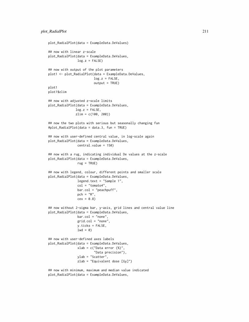
plot_RadialPlot 211

plot_RadialPlot(data = ExampleData.DeValues)

## now with linear z-scaleplot_RadialPlot(data = ExampleData.DeValues,

log.z = FALSE)

## now with output of the plot parametersplot1 <- plot_RadialPlot(data = ExampleData.DeValues,

log.z = FALSE,output = TRUE)

plot1plot1$zlim

## now with adjusted z-scale limitsplot_RadialPlot(data = ExampleData.DeValues,

log.z = FALSE,zlim = c(100, 200))

## now the two plots with serious but seasonally changing fun#plot_RadialPlot(data = data.3, fun = TRUE)

## now with user-defined central value, in log-scale againplot_RadialPlot(data = ExampleData.DeValues,

central.value = 150)

## now with a rug, indicating individual De values at the z-scaleplot_RadialPlot(data = ExampleData.DeValues,

rug = TRUE)

## now with legend, colour, different points and smaller scaleplot_RadialPlot(data = ExampleData.DeValues,

legend.text = "Sample 1",col = "tomato4",bar.col = "peachpuff",pch = "R",cex = 0.8)

## now without 2-sigma bar, y-axis, grid lines and central value lineplot_RadialPlot(data = ExampleData.DeValues,

bar.col = "none",grid.col = "none",y.ticks = FALSE,lwd = 0)

## now with user-defined axes labelsplot_RadialPlot(data = ExampleData.DeValues,

xlab = c("Data error (%)","Data precision"),

ylab = "Scatter",zlab = "Equivalent dose [Gy]")

## now with minimum, maximum and median value indicatedplot_RadialPlot(data = ExampleData.DeValues,

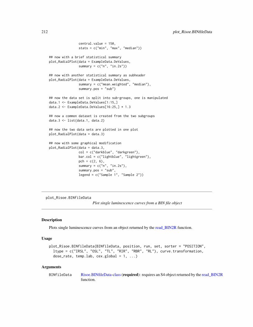
212 plot_Risoe.BINfileData

central.value = 150,stats = c("min", "max", "median"))

## now with a brief statistical summaryplot_RadialPlot(data = ExampleData.DeValues,

summary = c("n", "in.2s"))

## now with another statistical summary as subheaderplot_RadialPlot(data = ExampleData.DeValues,

summary = c("mean.weighted", "median"),summary.pos = "sub")

## now the data set is split into sub-groups, one is manipulateddata.1 <- ExampleData.DeValues[1:15,]data.2 <- ExampleData.DeValues[16:25,] * 1.3

## now a common dataset is created from the two subgroupsdata.3 <- list(data.1, data.2)

## now the two data sets are plotted in one plotplot_RadialPlot(data = data.3)

## now with some graphical modificationplot_RadialPlot(data = data.3,

col = c("darkblue", "darkgreen"),bar.col = c("lightblue", "lightgreen"),pch = c(2, 6),summary = c("n", "in.2s"),summary.pos = "sub",legend = c("Sample 1", "Sample 2"))

plot_Risoe.BINfileData

Plot single luminescence curves from a BIN file object

Description

Plots single luminescence curves from an object returned by the read_BIN2R function.

Usage

plot_Risoe.BINfileData(BINfileData, position, run, set, sorter = "POSITION",ltype = c("IRSL", "OSL", "TL", "RIR", "RBR", "RL"), curve.transformation,dose_rate, temp.lab, cex.global = 1, ...)

Arguments

BINfileData Risoe.BINfileData-class (required): requires an S4 object returned by the read_BIN2Rfunction.

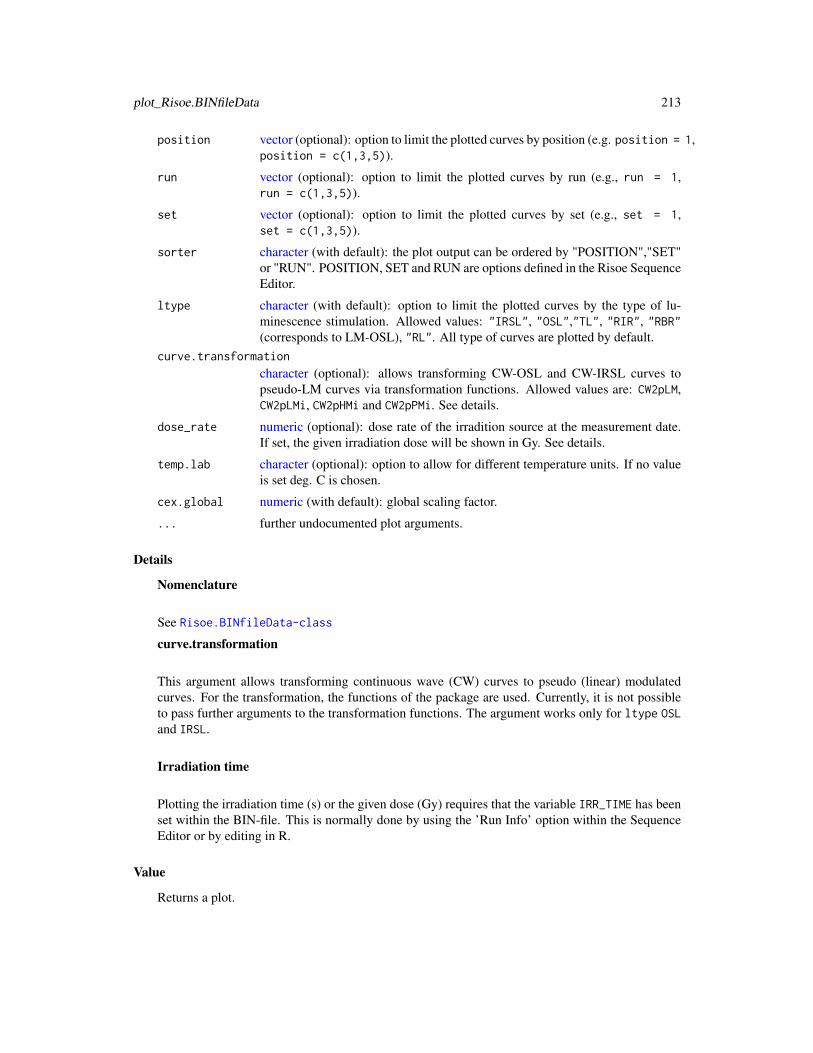
plot_Risoe.BINfileData 213

position vector (optional): option to limit the plotted curves by position (e.g. position = 1,position = c(1,3,5)).

run vector (optional): option to limit the plotted curves by run (e.g., run = 1,run = c(1,3,5)).

set vector (optional): option to limit the plotted curves by set (e.g., set = 1,set = c(1,3,5)).

sorter character (with default): the plot output can be ordered by "POSITION","SET"or "RUN". POSITION, SET and RUN are options defined in the Risoe SequenceEditor.

ltype character (with default): option to limit the plotted curves by the type of lu-minescence stimulation. Allowed values: "IRSL", "OSL","TL", "RIR", "RBR"(corresponds to LM-OSL), "RL". All type of curves are plotted by default.

curve.transformation

character (optional): allows transforming CW-OSL and CW-IRSL curves topseudo-LM curves via transformation functions. Allowed values are: CW2pLM,CW2pLMi, CW2pHMi and CW2pPMi. See details.

dose_rate numeric (optional): dose rate of the irradition source at the measurement date.If set, the given irradiation dose will be shown in Gy. See details.

temp.lab character (optional): option to allow for different temperature units. If no valueis set deg. C is chosen.


... further undocumented plot arguments.

Details

Nomenclature

See Risoe.BINfileData-class


This argument allows transforming continuous wave (CW) curves to pseudo (linear) modulatedcurves. For the transformation, the functions of the package are used. Currently, it is not possibleto pass further arguments to the transformation functions. The argument works only for ltype OSLand IRSL.

Irradiation time

Plotting the irradiation time (s) or the given dose (Gy) requires that the variable IRR_TIME has beenset within the BIN-file. This is normally done by using the ’Run Info’ option within the SequenceEditor or by editing in R.

Value

Returns a plot.

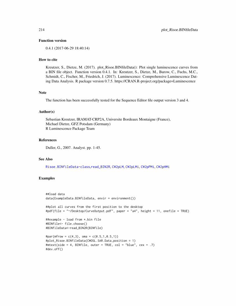
214 plot_Risoe.BINfileData

Function version

0.4.1 (2017-06-29 18:40:14)

How to cite

Kreutzer, S., Dietze, M. (2017). plot_Risoe.BINfileData(): Plot single luminescence curves froma BIN file object. Function version 0.4.1. In: Kreutzer, S., Dietze, M., Burow, C., Fuchs, M.C.,Schmidt, C., Fischer, M., Friedrich, J. (2017). Luminescence: Comprehensive Luminescence Dat-ing Data Analysis. R package version 0.7.5. https://CRAN.R-project.org/package=Luminescence

Note

The function has been successfully tested for the Sequence Editor file output version 3 and 4.

Author(s)

Sebastian Kreutzer, IRAMAT-CRP2A, Universite Bordeaux Montaigne (France),Michael Dietze, GFZ Potsdam (Germany)R Luminescence Package Team

References

Duller, G., 2007. Analyst. pp. 1-45.

See Also

Risoe.BINfileData-class,read_BIN2R, CW2pLM, CW2pLMi, CW2pPMi, CW2pHMi

Examples


##plot all curves from the first position to the desktop#pdf(file = "~/Desktop/CurveOutput.pdf", paper = "a4", height = 11, onefile = TRUE)

##example - load from *.bin file#BINfile<- file.choose()#BINfileData<-read_BIN2R(BINfile)

#par(mfrow = c(4,3), oma = c(0.5,1,0.5,1))#plot_Risoe.BINfileData(CWOSL.SAR.Data,position = 1)#mtext(side = 4, BINfile, outer = TRUE, col = "blue", cex = .7)#dev.off()

plot_RLum 215

plot_RLum General plot function for RLum S4 class objects

Description

Function calls object specific plot functions for RLum S4 class objects.

Usage

plot_RLum(object, ...)

Arguments

object RLum (required): S4 object of class RLum. Optional a list containing objectsof class RLum can be provided. In this case the function tries to plot every objectin this list according to its RLum class.

... further arguments and graphical parameters that will be passed to the specificplot functions. The only argument that is supported directly is main (setting theplot title). In contrast to the normal behaviour main can be here provided aslist and the arguments in the list will dispatched to the plots if the object isof type list as well.

Details

The function provides a generalised access point for plotting specific RLum objects.Depending on the input object, the corresponding plot function will be selected. Allowed argumentscan be found in the documentations of each plot function.

object corresponding plot functionRLum.Data.Curve : plot_RLum.Data.CurveRLum.Data.Spectrum : plot_RLum.Data.SpectrumRLum.Data.Image : plot_RLum.Data.ImageRLum.Analysis : plot_RLum.AnalysisRLum.Results : plot_RLum.Results

Value

Returns a plot.

Function version

0.4.3 (2017-06-29 18:40:14)

How to cite

Kreutzer, S. (2017). plot_RLum(): General plot function for RLum S4 class objects. Function ver-sion 0.4.3. In: Kreutzer, S., Dietze, M., Burow, C., Fuchs, M.C., Schmidt, C., Fischer, M., Friedrich,

216 plot_RLum.Analysis

J. (2017). Luminescence: Comprehensive Luminescence Dating Data Analysis. R package version0.7.5. https://CRAN.R-project.org/package=Luminescence

Note

The provided plot output depends on the input object.

Author(s)


References

#

See Also

plot_RLum.Data.Curve, RLum.Data.Curve, plot_RLum.Data.Spectrum, RLum.Data.Spectrum,plot_RLum.Data.Image, RLum.Data.Image, plot_RLum.Analysis, RLum.Analysis, plot_RLum.Results,RLum.Results

Examples

#load Example datadata(ExampleData.CW_OSL_Curve, envir = environment())

#transform data.frame to RLum.Data.Curve objecttemp <- as(ExampleData.CW_OSL_Curve, "RLum.Data.Curve")

#plot RLum objectplot_RLum(temp)

plot_RLum.Analysis Plot function for an RLum.Analysis S4 class object

Description

The function provides a standardised plot output for curve data of an RLum.Analysis S4 class object

Usage

plot_RLum.Analysis(object, subset = NULL, nrows, ncols, abline = NULL,combine = FALSE, curve.transformation, plot.single = FALSE, ...)

plot_RLum.Analysis 217

Arguments

object RLum.Analysis (required): S4 object of class RLum.Analysis

subset named list (optional): subsets elements for plotting. The arguments in thenamed list will be directly passed to the function get_RLum (e.g., subset = list(curveType = "measured"))

nrows integer (optional): sets number of rows for plot output, if nothing is set thefunction tries to find a value.

ncols integer (optional): sets number of columns for plot output, if nothing is set thefunction tries to find a value.

abline list (optional): allows to add ablines to the plot. Argument are provided in a listand will be forwared to the function abline, e.g., list(v = c(10, 100)) addstwo vertical lines add 10 and 100 to all plots. In contrast list(v = c(10), v = c(100)adds a vertical at 10 to the first and a vertical line at 100 to the 2nd plot.

combine logical (with default): allows to combine all RLum.Data.Curve objects in onesingle plot.


character (optional): allows transforming CW-OSL and CW-IRSL curves topseudo-LM curves via transformation functions. Allowed values are: CW2pLM,CW2pLMi, CW2pHMi and CW2pPMi. See details.

plot.single logical (with default): global par settings are considered, normally this shouldend in one plot per page

... further arguments and graphical parameters will be passed to the plot func-tion. Supported arguments: main, mtext, log, lwd, lty type, pch, col, norm,xlim,ylim, xlab, ylab... and for combine = TRUE also: sub, legend, legend.text,legend.pos (typical plus ’outside’), legend.col, smooth. All arguments canbe provided as vector or list to gain in full control of all plot settings.

Details

The function produces a multiple plot output. A file output is recommended (e.g., pdf).


This argument allows transforming continuous wave (CW) curves to pseudo (linear) modulatedcurves. For the transformation, the functions of the package are used. Currently, it is not possibleto pass further arguments to the transformation functions. The argument works only for ltype OSLand IRSL.

Please note: The curve transformation within this functions works roughly, i.e. every IRSL or OSLcurve is transformed, without considerung whether it is measured with the PMT or not! However,for a fast look it might be helpful.

Value

Returns multiple plots.

218 plot_RLum.Analysis

Function version

0.3.8 (2017-06-29 18:40:14)

How to cite

Kreutzer, S. (2017). plot_RLum.Analysis(): Plot function for an RLum.Analysis S4 class object.Function version 0.3.8. In: Kreutzer, S., Dietze, M., Burow, C., Fuchs, M.C., Schmidt, C., Fischer,M., Friedrich, J. (2017). Luminescence: Comprehensive Luminescence Dating Data Analysis. Rpackage version 0.7.5. https://CRAN.R-project.org/package=Luminescence

Note

Not all arguments available for plot will be passed! Only plotting of RLum.Data.Curve andRLum.Data.Spectrum objects are currently supported.

Author(s)


References

#

See Also

plot, plot_RLum, plot_RLum.Data.Curve

Examples


##convert values for position 1temp <- Risoe.BINfileData2RLum.Analysis(CWOSL.SAR.Data, pos=1)

##(1) plot (combine) TL curves in one plotplot_RLum.Analysis(temp,subset = list(recordType = "TL"),combine = TRUE,norm = TRUE,abline = list(v = c(110)))

##(2) same as example (1) but using## the argument smooth = TRUEplot_RLum.Analysis(temp,

plot_RLum.Data.Curve 219

subset = list(recordType = "TL"),combine = TRUE,norm = TRUE,smooth = TRUE,abline = list(v = c(110)))

plot_RLum.Data.Curve Plot function for an RLum.Data.Curve S4 class object

Description

The function provides a standardised plot output for curve data of an RLum.Data.Curve S4 classobject

Usage

plot_RLum.Data.Curve(object, par.local = TRUE, norm = FALSE,smooth = FALSE, ...)

Arguments

object RLum.Data.Curve (required): S4 object of class RLum.Data.Curve

par.local logical (with default): use local graphical parameters for plotting, e.g. the plotis shown in one column and one row. If par.local = FALSE, global parametersare inherited.

norm logical (with default): allows curve normalisation to the highest count value

smooth logical (with default): provides an automatic curve smoothing based on rollmean

... further arguments and graphical parameters that will be passed to the plot func-tion

Details

Only single curve data can be plotted with this function. Arguments according to plot.

Value

Returns a plot.

Function version

0.2.3 (2017-06-29 18:40:14)

220 plot_RLum.Data.Image

How to cite

Kreutzer, S. (2017). plot_RLum.Data.Curve(): Plot function for an RLum.Data.Curve S4 classobject. Function version 0.2.3. In: Kreutzer, S., Dietze, M., Burow, C., Fuchs, M.C., Schmidt,C., Fischer, M., Friedrich, J. (2017). Luminescence: Comprehensive Luminescence Dating DataAnalysis. R package version 0.7.5. https://CRAN.R-project.org/package=Luminescence

Note

Not all arguments of plot will be passed!

Author(s)


References

#

See Also

plot, plot_RLum

Examples

##plot curve data

#load Example datadata(ExampleData.CW_OSL_Curve, envir = environment())

#transform data.frame to RLum.Data.Curve objecttemp <- as(ExampleData.CW_OSL_Curve, "RLum.Data.Curve")

#plot RLum.Data.Curve objectplot_RLum.Data.Curve(temp)

plot_RLum.Data.Image Plot function for an RLum.Data.Image S4 class object

Description

The function provides a standardised plot output for image data of an RLum.Data.ImageS4 classobject, mainly using the plot functions provided by the raster package.

plot_RLum.Data.Image 221

Usage

plot_RLum.Data.Image(object, par.local = TRUE, plot.type = "plot.raster",...)

Arguments

object RLum.Data.Image (required): S4 object of class RLum.Data.Image

par.local logical (with default): use local graphical parameters for plotting, e.g. the plotis shown in one column and one row. If par.local = FALSE global parametersare inherited.

plot.type character (with default): plot types. Supported types are plot.raster, plotRGBor contour

... further arguments and graphical parameters that will be passed to the specificplot functions.

Details

Details on the plot functions

Image is visualised as 2D plot usinng generic plot types provided by other packages.

Supported plot types:

plot.type = "plot.raster"

Uses the standard plot function for raster data from the package raster: plot. For each raster layerin a raster brick one plot is produced.

Arguments that are passed through the function call:

main,axes, xlab, ylab, xlim, ylim, col

plot.type = "plotRGB"

Uses the function plotRGB from the raster package. Only one image plot is produced as all layersin a brick a combined. This plot type is useful to see whether any signal is recorded by the camera.Arguments that are passed through the function call:

main,axes, xlab, ylab, ext, interpolate, maxpixels, alpha, colNA, stretch

plot.type = "contour"

Uses the function contour plot function from the raster function (contour). For each raster layerone contour plot is produced. Arguments that are passed through the function call:

main,axes, xlab, ylab, xlim, ylim, col

222 plot_RLum.Data.Image

Value

Returns a plot.

Function version

0.1 (2017-06-29 18:40:14)

How to cite

Kreutzer, S. (2017). plot_RLum.Data.Image(): Plot function for an RLum.Data.Image S4 classobject. Function version 0.1. In: Kreutzer, S., Dietze, M., Burow, C., Fuchs, M.C., Schmidt,C., Fischer, M., Friedrich, J. (2017). Luminescence: Comprehensive Luminescence Dating DataAnalysis. R package version 0.7.5. https://CRAN.R-project.org/package=Luminescence

Note

This function has been created to faciliate the plotting of image data imported by the functionread_SPE2R. However, so far the function is not optimized to handle image data > ca. 200 MByteand thus plotting of such data is extremely slow.

Author(s)


References

-

See Also

RLum.Data.Image, plot, plot_RLum, raster,

Examples

##load datadata(ExampleData.RLum.Data.Image, envir = environment())

##plot dataplot_RLum.Data.Image(ExampleData.RLum.Data.Image)

plot_RLum.Data.Spectrum 223

plot_RLum.Data.Spectrum

Plot function for an RLum.Data.Spectrum S4 class object

Description

The function provides a standardised plot output for spectrum data of an RLum.Data.Spectrum S4class object

Usage

plot_RLum.Data.Spectrum(object, par.local = TRUE, plot.type = "contour",optical.wavelength.colours = TRUE, bg.channels, bin.rows = 1,bin.cols = 1, rug = TRUE, limit_counts = NULL, xaxis.energy = FALSE,legend.text, ...)

Arguments

object RLum.Data.Spectrum or matrix (required): S4 object of class RLum.Data.Spectrumor a matrix containing count values of the spectrum.Please note that in case of a matrix rownames and colnames are set automaticallyif not provided.

par.local logical (with default): use local graphical parameters for plotting, e.g. the plotis shown in one column and one row. If par.local = FALSE global parametersare inherited.

plot.type character (with default): plot type, for 3D-plot use persp, or interactive,for a 2D-plot contour, single or multiple.lines (along the time or temper-ature axis) or transect (along the wavelength axis)

optical.wavelength.colours

logical (with default): use optical wavelength colour palette. Note: For this,the spectrum range is limited: c(350,750). Own colours can be set with theargument col.

bg.channels vector (optional): defines channel for background subtraction If a vector isprovided the mean of the channels is used for subtraction. Note: Backgroundsubtraction is applied prior to channel binning

bin.rows integer (with defaul): allow summing-up wavelength channels (horizontal bin-ning), e.g. bin.rows = 2 two channels are summed up

bin.cols integer (with default): allow summing-up channel counts (vertical binning) forplotting, e.g. bin.cols = 2 two channels are summed up

rug logical (with default): enables or disables colour rug. Currently only imple-mented for plot type multiple.lines and single

limit_counts numeric (optional): value to limit all count values to this value, i.e. all countvalues above this threshold will be replaced by this threshold. This is helpfullespecially in case of TL-spectra.

224 plot_RLum.Data.Spectrum

xaxis.energy logical (with default): enables or disables energy instead of wavelength axis.Note: This option means not only simnply redrawing the axis, insteadly thespectrum in terms of intensity is recalculated, s. details.

legend.text character (with default): possiblity to provide own legend text. This argumentis only considered for plot types providing a legend, e.g. plot.type="transect"

... further arguments and graphical parameters that will be passed to the plot func-tion.

Details

Matrix structure(cf. RLum.Data.Spectrum)

• rows (x-values): wavelengths/channels (xlim, xlab)

• columns (y-values): time/temperature (ylim, ylab)

• cells (z-values): count values (zlim, zlab)

Note: This nomenclature is valid for all plot types of this function!

Nomenclature for value limitingxlim: Limits values along the wavelength axisylim: Limits values along the time/temperature axiszlim: Limits values along the count value axis

Energy axis re-calculationIf the argument xaxis.energy = TRUE is chosen, instead intensity vs. wavelength the spectrum isplotted as intensiyt vs. energy. Therefore the entire spectrum is re-recaluated (e.g., Appendix 4 inBlasse and Grabmeier, 1994):

The intensity of the spectrum (z-values) is re-calcualted using the following equation:

φE = φλ ∗ λ2/(hc)

with φE the intensity per interval of energy E (eV), φλ the intensity per interval of wavelength λ(nm) and h (eV/s) the Planck constant and c (m/s) the velocity of light.

For transforming the wavelength axis (x-values) the equation

E = hc/λ

is used. For further details please see the cited the literature.

Details on the plot functionsSpectrum is visualised as 3D or 2D plot. Both plot types are based on internal R plot functions.

plot.type = "persp"

Arguments that will be passed to persp:

plot_RLum.Data.Spectrum 225

• shade: default is 0.4

• phi: default is 15

• theta: default is -30

• expand: default is 1

• ticktype: default is detailed, r: default is 10

Note: Further parameters can be adjusted via par. For example to set the background transparentand reduce the thickness of the lines use: par(bg = NA, lwd = 0.7) previous the function call.

plot.type = "single"

Per frame a single curve is returned. Frames are time or temperature steps.

plot.type = "multiple.lines"

All frames plotted in one frame.

plot.type = "transect"

Depending on the selected wavelength/channel range a transect over the time/temperature (y-axis)will be plotted along the wavelength/channels (x-axis). If the range contains more than one channel,values (z-values) are summed up. To select a transect use the xlim argument, e.g. xlim = c(300,310)plot along the summed up count values of channel 300 to 310.

Further arguments that will be passed (depending on the plot type)xlab, ylab, zlab, xlim, ylim, zlim, main, mtext, pch, type ("single", "multiple.lines", "interac-tive"), col, border, box lwd, bty, showscale ("interactive")

Value

Returns a plot.

Function version

0.5.3 (2017-06-29 18:40:14)

How to cite

Kreutzer, S. (2017). plot_RLum.Data.Spectrum(): Plot function for an RLum.Data.Spectrum S4class object. Function version 0.5.3. In: Kreutzer, S., Dietze, M., Burow, C., Fuchs, M.C., Schmidt,C., Fischer, M., Friedrich, J. (2017). Luminescence: Comprehensive Luminescence Dating DataAnalysis. R package version 0.7.5. https://CRAN.R-project.org/package=Luminescence

Note

Not all additional arguments (...) will be passed similarly!

226 plot_RLum.Data.Spectrum

Author(s)


References

Blasse, G., Grabmaier, B.C., 1994. Luminescent Materials. Springer.

See Also

RLum.Data.Spectrum, plot, plot_RLum, persp, plot_ly, contour

Examples


##(1)plot simple spectrum (2D) - contourplot_RLum.Data.Spectrum(TL.Spectrum,

plot.type="contour",xlim = c(310,750),ylim = c(0,300),bin.rows=10,bin.cols = 1)

##(2) plot spectrum (3D)plot_RLum.Data.Spectrum(TL.Spectrum,

plot.type="persp",xlim = c(310,750),ylim = c(0,100),bin.rows=10,bin.cols = 1)

##(3) plot multiple lines (2D) - multiple.lines (with ylim)plot_RLum.Data.Spectrum(TL.Spectrum,

plot.type="multiple.lines",xlim = c(310,750),ylim = c(0,100),bin.rows=10,bin.cols = 1)

## Not run:##(4) interactive plot using the package plotly ("surface")plot_RLum.Data.Spectrum(TL.Spectrum, plot.type="interactive",xlim = c(310,750), ylim = c(0,300), bin.rows=10,bin.cols = 1)

##(5) interactive plot using the package plotly ("contour")plot_RLum.Data.Spectrum(TL.Spectrum, plot.type="interactive",xlim = c(310,750), ylim = c(0,300), bin.rows=10,

plot_RLum.Results 227

bin.cols = 1,type = "contour",showscale = TRUE)

##(6) interactive plot using the package plotly ("heatmap")plot_RLum.Data.Spectrum(TL.Spectrum, plot.type="interactive",xlim = c(310,750), ylim = c(0,300), bin.rows=10,bin.cols = 1,type = "heatmap",showscale = TRUE)

##(7) alternative using the package fieldsfields::image.plot(get_RLum(TL.Spectrum))contour(get_RLum(TL.Spectrum), add = TRUE)

## End(Not run)

plot_RLum.Results Plot function for an RLum.Results S4 class object

Description

The function provides a standardised plot output for data of an RLum.Results S4 class object

Usage

plot_RLum.Results(object, single = TRUE, ...)

Arguments

object RLum.Results (required): S4 object of class RLum.Results

single logical (with default): single plot output (TRUE/FALSE) to allow for plottingthe results in as few plot windows as possible.

... further arguments and graphical parameters will be passed to the plot function.

Details

The function produces a multiple plot output. A file output is recommended (e.g., pdf).

Value

Returns multiple plots.

Function version

0.2.1 (2017-06-29 18:40:14)

228 plot_RLum.Results

How to cite

Burow, C., Kreutzer, S. (2017). plot_RLum.Results(): Plot function for an RLum.Results S4 classobject. Function version 0.2.1. In: Kreutzer, S., Dietze, M., Burow, C., Fuchs, M.C., Schmidt,C., Fischer, M., Friedrich, J. (2017). Luminescence: Comprehensive Luminescence Dating DataAnalysis. R package version 0.7.5. https://CRAN.R-project.org/package=Luminescence

Note

Not all arguments available for plot will be passed! Only plotting of RLum.Results objects aresupported.

Author(s)

Christoph Burow, University of Cologne (Germany), Sebastian Kreutzer, IRAMAT-CRP2A, Uni-versite Bordeaux Montaigne (France)R Luminescence Package Team

References

#

See Also

plot, plot_RLum,

Examples

###load datadata(ExampleData.DeValues, envir = environment())

# apply the un-logged minimum age modelmam <- calc_MinDose(data = ExampleData.DeValues$CA1, sigmab = 0.2, log = TRUE, plot = FALSE)

##plotplot_RLum.Results(mam)

# estimate the number of grains on an aliquotgrains<- calc_AliquotSize(grain.size = c(100,150), sample.diameter = 1, plot = FALSE, MC.iter = 100)

##plotplot_RLum.Results(grains)

plot_ViolinPlot 229

plot_ViolinPlot Create a violin plot

Description

Draws a kernal densiy plot in combination with a boxplot in its middle. The shape of the violinis constructed using a mirrored density curve. This plot is especially designed for cases where theindividual errors are zero or to small to be visualised. The idea for this plot is based on the the’volcano plot’ in the ggplot2 package by Hadely Wickham and Winston Chang. The general ideafor the Violin Plot seems to be introduced by Hintze and Nelson (1998).

Usage

plot_ViolinPlot(data, boxplot = TRUE, rug = TRUE, summary = NULL,summary.pos = "sub", na.rm = TRUE, ...)

Arguments

data numeric or RLum.Results object (required): input data for plotting. Alterna-tively a data.frame or a matrix can be provided, but only the first column willbe considered by the function

boxplot logical (with default): enable or disable boxplotrug logical (with default): enable or disable rugsummary character (optional): add statistic measures of centrality and dispersion to the

plot. Can be one or more of several keywords. See details for available key-words.

summary.pos numeric or character (with default): optional position keywords (cf., legend)for the statistical summary. Alternatively, the keyword "sub" may be specifiedto place the summary below the plot header. However, this latter option in onlypossible if mtext is not used.

na.rm logical (with default): exclude NA values from the data set prior to any furtheroperations.

... further arguments and graphical parameters passed to plot.default, densityand boxplot. See details for further information

Details

The function is passing several arguments to the function plot, density, boxplot: Supportedarguments are: xlim, main, xlab, ylab, col.violin, col.boxplot, mtext, cex, mtext

Valid summary keywords

’n’, ’mean’, ’median’, ’sd.abs’, ’sd.rel’, ’se.abs’, ’se.rel’, ’skewness’, ’kurtosis’

Function version

0.1.3 (2017-06-29 18:40:14)

230 plot_ViolinPlot

How to cite

Kreutzer, S. (2017). plot_ViolinPlot(): Create a violin plot. Function version 0.1.3. In: Kreutzer, S.,Dietze, M., Burow, C., Fuchs, M.C., Schmidt, C., Fischer, M., Friedrich, J. (2017). Luminescence:Comprehensive Luminescence Dating Data Analysis. R package version 0.7.5. https://CRAN.R-project.org/package=Luminescence

Note

Although the code for this function was developed independently and just the idea for the plot wasbased on the ’ggplot2’ package plot type ’volcano’, it should be mentioned that, beyond this, twoother R packages exist providing a possibility to produces this kind of plot, namely: ’vioplot’ and’violinmplot’ (see References for details).

Author(s)


References

Daniel Adler (2005). vioplot: A violin plot is a combination of a box plot and a kernel density plot.R package version 0.2 http://CRAN.R-project.org/package=violplot

Hintze, J.L., Nelson, R.D., 1998. A Box Plot-Density Trace Synergism. The American Statistician52, 181-184.

Raphael W. Majeed (2012). violinmplot: Combination of violin plot with mean and standard devi-ation. R package version 0.2.1. http://CRAN.R-project.org/package=violinmplot

Wickham. H (2009). ggplot2: elegant graphics for data analysis. Springer New York.

See Also

density, plot, boxplot, rug, calc_Statistics

Examples

## read example data setdata(ExampleData.DeValues, envir = environment())ExampleData.DeValues <- Second2Gray(ExampleData.DeValues$BT998, c(0.0438,0.0019))

## create plot straightforwardplot_ViolinPlot(data = ExampleData.DeValues)

PSL2Risoe.BINfileData 231

PSL2Risoe.BINfileData Convert portable OSL data to an Risoe.BINfileData object

Description

Converts an RLum.Analysis object produced by the function read_PSL2R() to an Risoe.BINfileDataobject (BETA).

Usage

PSL2Risoe.BINfileData(object, ...)

Arguments

object RLum.Analysis (required): RLum.Analysis object produced by read_PSL2R


Details

This function converts an RLum.Analysis object that was produced by the read_PSL2R functionto an Risoe.BINfileData. The Risoe.BINfileData can be used to write a Risoe BIN file viawrite_R2BIN.

Value

Returns an S4 Risoe.BINfileData object that can be used to write a BIN file using write_R2BIN.

Function version

0.0.1 (2017-06-29 18:40:14)

How to cite

Burow, C. (2017). PSL2Risoe.BINfileData(): Convert portable OSL data to an Risoe.BINfileDataobject. Function version 0.0.1. In: Kreutzer, S., Dietze, M., Burow, C., Fuchs, M.C., Schmidt,C., Fischer, M., Friedrich, J. (2017). Luminescence: Comprehensive Luminescence Dating DataAnalysis. R package version 0.7.5. https://CRAN.R-project.org/package=Luminescence

Author(s)


See Also

RLum.Analysis, RLum.Data.Curve, Risoe.BINfileData

232 read_BIN2R

Examples

# (1) load and plot example data setdata("ExampleData.portableOSL", envir = environment())plot_RLum(ExampleData.portableOSL)

# (2) merge all RLum.Analysis objects into onemerged <- merge_RLum(ExampleData.portableOSL)merged

# (3) convert to RisoeBINfile objectbin <- PSL2Risoe.BINfileData(merged)bin

# (4) write Risoe BIN file## Not run:write_R2BIN(bin, "~/portableOSL.binx")

## End(Not run)

read_BIN2R Import Risoe BIN-file into R

Description

Import a *.bin or a *.binx file produced by a Risoe DA15 and DA20 TL/OSL reader into R.

Usage

read_BIN2R(file, show.raw.values = FALSE, position = NULL,n.records = NULL, zero_data.rm = TRUE, duplicated.rm = FALSE,fastForward = FALSE, show.record.number = FALSE, txtProgressBar = TRUE,forced.VersionNumber = NULL, ignore.RECTYPE = FALSE, pattern = NULL,verbose = TRUE, ...)

Arguments

file character or list (required): path and file name of the BIN/BINX file (URLsare supported). If input is a list it should comprise only characters represent-ing each valid path and BIN/BINX-file names. Alternatively the input charactercan be just a directory (path), in this case the the function tries to detect andimport all BIN/BINX files found in the directory.

show.raw.values

logical (with default): shows raw values from BIN file for LTYPE, DTYPE andLIGHTSOURCE without translation in characters. Can be provided as list if fileis a list.

read_BIN2R 233

position numeric (optional): imports only the selected position. Note: the import perfor-mance will not benefit by any selection made here. Can be provided as list iffile is a list.

n.records raw (optional): limits the number of imported records. Can be used in combina-tion with show.record.number for debugging purposes, e.g. corrupt BIN-files.Can be provided as list if file is a list.

zero_data.rm logical (with default): remove erroneous data with no count values. As suchdata are usally not needed for the subsequent data analysis they will be removedby default. Can be provided as list if file is a list.

duplicated.rm logical (with default): remove duplicated entries if TRUE. This may happendue to an erroneous produced BIN/BINX-file. This option compares only pre-deccessor and successor. Can be provided as list if file is a list.

fastForward logical (with default): if TRUE for a more efficient data processing only a list ofRLum.Analysis objects is returned instead of a Risoe.BINfileData-class object.Can be provided as list if file is a list.

show.record.number

logical (with default): shows record number of the imported record, for debug-ging usage only. Can be provided as list if file is a list.

txtProgressBar logical (with default): enables or disables txtProgressBar.forced.VersionNumber

integer (optional): allows to cheat the version number check in the functionby own values for cases where the BIN-file version is not supported. Can beprovided as list if file is a list.Note: The usage is at own risk, only supported BIN-file versions have beentested.

ignore.RECTYPE logical (with default): this argument allows to ignore values in the byte ’REG-TYPE’ (BIN-file version 08), in case there are not documented or faulty set. Ifset all records are treated like records of ’REGYPE’ 0 or 1.

pattern character (optional): argument that is used if only a path is provided. Theargument will than be passed to the function list.files used internally toconstruct a list of wanted files

verbose logical (with default): enables or disables verbose mode

... further arguments that will be passed to the function Risoe.BINfileData2RLum.Analysis.Please note that any matching argument automatically sets fastForward = TRUE

Details

The binary data file is parsed byte by byte following the data structure published in the Appendicesof the Analyst manual p. 42.

For the general BIN-file structure, the reader is referred to the Risoe website: http://www.nutech.dtu.dk/

Value

Returns an S4 Risoe.BINfileData-class object containing two slots:

234 read_BIN2R

METADATA A data.frame containing all variables stored in the bin-file.

DATA A list containing a numeric vector of the measured data. The ID corresponds tothe record ID in METADATA.

If fastForward = TRUE a list of RLum.Analysis object is returned. The internal coercing is doneusing the function Risoe.BINfileData2RLum.Analysis

Function version

0.15.6 (2017-06-29 18:40:14)

How to cite

Kreutzer, S., Fuchs, M.C., Fuchs, M. (2017). read_BIN2R(): Import Risoe BIN-file into R. Func-tion version 0.15.6. In: Kreutzer, S., Dietze, M., Burow, C., Fuchs, M.C., Schmidt, C., Fischer,M., Friedrich, J. (2017). Luminescence: Comprehensive Luminescence Dating Data Analysis. Rpackage version 0.7.5. https://CRAN.R-project.org/package=Luminescence

Note

The function works for BIN/BINX-format versions 03, 04, 06, 07 and 08. The version numberdepends on the used Sequence Editor.

ROI data sets introduced with BIN-file version 8 are not supported and skipped durint import.

Author(s)

Sebastian Kreutzer, IRAMAT-CRP2A, Universite Bordeaux Montaigne (France), Margret C. Fuchs,HZDR Freiberg, (Germany)R Luminescence Package Team

References

DTU Nutech, 2016. The Squence Editor, Users Manual, February, 2016. http://www.nutech.dtu.dk/english/products-and-services/radiation-instruments/tl_osl_reader/manuals

See Also

write_R2BIN, Risoe.BINfileData, readBin, merge_Risoe.BINfileData, RLum.Analysis txtProgressBar,list.files

Examples

##(1) import Risoe BIN-file to R (uncomment for usage)

#FILE <- file.choose()

http://www.nutech.dtu.dk/english/products-and-services/radiation-instruments/tl_osl_reader/manuals


read_Daybreak2R 235

#temp <- read_BIN2R(FILE)#temp

read_Daybreak2R Import measurement data produced by a Daybreak TL/OSL readerinto R

Description

Import a TXT-file (ASCII file) or a DAT-file (binary file) produced by a Daybreak reader into R.The import of the DAT-files is limited to the file format described for the software TLAPLLIC v.3.2used for a Daybreak, model 1100.

Usage

read_Daybreak2R(file, raw = FALSE, verbose = TRUE, txtProgressBar = TRUE)

Arguments

file character or list (required): path and file name of the file to be imported.Alternatively a list of file names can be provided or just the path a folder contain-ing measurement data. Please note that the specific, common, file extension (txt)is likely leading to function failures during import when just a path is provided.

raw logical (with default): if the input is a DAT-file (binary) a data.table insteadof the RLum.Analysis object can be returned for debugging purposes.

verbose logical (with default): enables or disables terminal feedback

txtProgressBar logical (with default): enables or disables txtProgressBar.

Value

A list of RLum.Analysis objects (each per position) is provided.

Function version

0.3.0 (2017-06-29 18:40:14)

How to cite

Kreutzer, S., Zink, A. (2017). read_Daybreak2R(): Import measurement data produced by a Day-break TL/OSL reader into R. Function version 0.3.0. In: Kreutzer, S., Dietze, M., Burow, C., Fuchs,M.C., Schmidt, C., Fischer, M., Friedrich, J. (2017). Luminescence: Comprehensive LuminescenceDating Data Analysis. R package version 0.7.5. https://CRAN.R-project.org/package=Luminescence

Note

[BETA VERSION] This function still needs to be tested properly. In particular the function hasunderwent only very rough rests using a few files.

236 read_PSL2R

Author(s)

Sebastian Kreutzer, IRAMAT-CRP2A, Universite Bordeaux Montaigne (France),Anotine Zink, C2RMF, Palais du Louvre, Paris (France)

The ASCII-file import is based on a suggestion by Willian Amidon and Andrew Louis GorinR Luminescence Package Team

References

-

See Also

RLum.Analysis, RLum.Data.Curve, data.table

Examples

## Not run:file <- file.choose()temp <- read_Daybreak2R(file)

## End(Not run)

read_PSL2R Import PSL files to R

Description

Imports PSL files produced by a SUERC portable OSL reader into R (BETA).

Usage

read_PSL2R(file, drop_bg = FALSE, as_decay_curve = TRUE, smooth = FALSE,merge = FALSE, ...)

Arguments

file character (required): path and file name of the PSL file. If input is a vector itshould comprise only characters representing valid paths and PSL file names.Alternatively the input character can be just a directory (path). In this case thethe function tries to detect and import all PSL files found in the directory.

drop_bg logical (with default): TRUE to automatically remove all non-OSL/IRSL curves.

as_decay_curve logical (with default): Portable OSL Reader curves are often given as cumula-tive light sum curves. Use TRUE (default) to convert the curves to the more usualdecay form.

read_PSL2R 237

smooth logical (with default): TRUE to apply Tukey’s Running Median Smoothing forOSL and IRSL decay curves. Smoothing is encouraged if you see random signaldrops within the decay curves related to hardware errors.

merge logical (with default): TRUE to merge all RLum.Analysis objects. Only appli-cable if multiple files are imported.


Details

This function provides an import routine for the SUERC portable OSL Reader PSL format. PSLfiles are just plain text and can be viewed with any text editor. Due to the formatting of PSL filesthis import function relies heavily on regular expression to find and extract all relevant information.See note.

Value

Returns an S4 RLum.Analysis object containing RLum.Data.Curve objects for each curve.

Function version

0.0.1 (2017-06-29 18:40:14)

How to cite

Burow, C. (2017). read_PSL2R(): Import PSL files to R. Function version 0.0.1. In: Kreutzer, S.,Dietze, M., Burow, C., Fuchs, M.C., Schmidt, C., Fischer, M., Friedrich, J. (2017). Luminescence:Comprehensive Luminescence Dating Data Analysis. R package version 0.7.5. https://CRAN.R-project.org/package=Luminescence

Note

Because this function relies heavily on regular expressions to parse PSL files it is currently only inbeta status. If the routine fails to import a specific PSL file please report to <[email protected]> so the function can be updated.

Author(s)


See Also

RLum.Analysis, RLum.Data.Curve, RLum.Data.Curve

238 read_SPE2R

Examples

# (1) Import PSL file to R

## Not run:FILE <- file.choose()temp <- read_PSL2R(FILE)temp

## End(Not run)

read_SPE2R Import Princeton Intruments (TM) SPE-file into R

Description

Function imports Princeton Instruments (TM) SPE-files into R environment and provides RLumobjects as output.

Usage

read_SPE2R(file, output.object = "RLum.Data.Image", frame.range,txtProgressBar = TRUE)

Arguments

file character (required): spe-file name (including path), e.g.[WIN]: read_SPE2R("C:/Desktop/test.spe"),[MAC/LINUX]: readSPER("/User/test/Desktop/test.spe")

output.object character (with default): set RLum output object. Allowed types are "RLum.Data.Spectrum","RLum.Data.Image" or "matrix"

frame.range vector (optional): limit frame range, e.g. select first 100 frames by frame.range = c(1,100)


Details

Function provides an import routine for the Princton Instruments SPE format. Import functionalityis based on the file format description provided by Princton Instruments and a MatLab script writtenby Carl Hall (s. references).

read_SPE2R 239

Value

Depending on the chosen option the functions returns three different type of objects:

output.object.

RLum.Data.Spectrum

An object of type RLum.Data.Spectrum is returned. Row sums are used to integrate all counts overone channel.

RLum.Data.Image

An object of type RLum.Data.Image is returned. Due to performace reasons the import is abortedfor files containing more than 100 frames. This limitation can be overwritten manually by using theargument frame.frange.

matrix

Returns a matrix of the form: Rows = Channels, columns = Frames. For the transformation thefunction get_RLum is used, meaning that the same results can be obtained by using the functionget_RLum on an RLum.Data.Spectrum or RLum.Data.Image object.

Function version

0.1.0 (2017-06-29 18:40:14)

How to cite

Kreutzer, S. (2017). read_SPE2R(): Import Princeton Intruments (TM) SPE-file into R. Functionversion 0.1.0. In: Kreutzer, S., Dietze, M., Burow, C., Fuchs, M.C., Schmidt, C., Fischer, M.,Friedrich, J. (2017). Luminescence: Comprehensive Luminescence Dating Data Analysis. R pack-age version 0.7.5. https://CRAN.R-project.org/package=Luminescence

Note

The function does not test whether the input data are spectra or pictures for spatial resolvedanalysis!

The function has been successfully tested for SPE format versions 2.x.

Currently not all information provided by the SPE format are supported.

Author(s)


240 read_XSYG2R

References

Princeton Instruments, 2014. Princeton Instruments SPE 3.0 File Format Specification, Version 1.A(for document URL please use an internet search machine)

Hall, C., 2012: readSPE.m. http://www.mathworks.com/matlabcentral/fileexchange/35940-readspe/content/readSPE.m

See Also

readBin, RLum.Data.Spectrum, raster

Examples

## to run examples uncomment lines and run the code

##(1) Import data as RLum.Data.Spectrum object#file <- file.choose()#temp <- read_SPE2R(file)#temp

##(2) Import data as RLum.Data.Image object#file <- file.choose()#temp <- read_SPE2R(file, output.object = "RLum.Data.Image")#temp

##(3) Import data as matrix object#file <- file.choose()#temp <- read_SPE2R(file, output.object = "matrix")#temp

##(4) Export raw data to csv, if temp is a RLum.Data.Spectrum object# write.table(x = get_RLum(temp),# file = "[your path and filename]",# sep = ";", row.names = FALSE)

read_XSYG2R Import XSYG files to R

Description

Imports XSYG files produced by a Freiberg Instrument lexsyg reader into R.

Usage

read_XSYG2R(file, recalculate.TL.curves = TRUE, fastForward = FALSE,import = TRUE, pattern = ".xsyg", txtProgressBar = TRUE)

http://www.mathworks.com/matlabcentral/fileexchange/35940-readspe/content/readSPE.m

http://www.mathworks.com/matlabcentral/fileexchange/35940-readspe/content/readSPE.m

read_XSYG2R 241

Arguments

file character or list (required): path and file name of the XSYG file. If inputis a list it should comprise only characters representing each valid path andxsyg-file names. Alternatively the input character can be just a directory (path),in this case the the function tries to detect and import all xsyg files found in thedirectory.

recalculate.TL.curves

logical (with default): if set to TRUE, TL curves are returned as temperatureagainst count values (see details for more information) Note: The option over-writes the time vs. count TL curve. Select FALSE to import the raw data deliveredby the lexsyg. Works for TL curves and spectra.

fastForward logical (with default): if TRUE for a more efficient data processing only a listof RLum.Analysis objects is returned.

import logical (with default): if set to FALSE, only the XSYG file structure is shown.

pattern regex (with default): optional regular expression if file is a link to a folder, toselect just specific XSYG-files

txtProgressBar logical (with default): enables TRUE or disables FALSE the progression bar duringimport

Details

How does the import function work?

The function uses the xml package to parse the file structure. Each sequence is subsequently trans-lated into an RLum.Analysis object.

General structure XSYG format

<?xml?<Sample><Sequence><Record><Curve name="first curve" /><Curve name="curve with data">x0 , y0 ; x1 , y1 ; x2 , y2 ; x3 , y3</Curve></Record></Sequence></Sample>

So far, each XSYG file can only contain one <Sample></Sample>, but multiple sequences.

Each record may comprise several curves.

242 read_XSYG2R

TL curve recalculation

On the FI lexsyg device TL curves are recorded as time against count values. Temperature valuesare monitored on the heating plate and stored in a separate curve (time vs. temperature). If theoption recalculate.TL.curves = TRUE is chosen, the time values for each TL curve are replacedby temperature values.

Practically, this means combining two matrices (Time vs. Counts and Time vs. Temperature) withdifferent row numbers by their time values. Three cases are considered:

HE: Heating elementPMT: Photomultiplier tubeInterpolation is done using the function approx

CASE (1): nrow(matrix(PMT)) > nrow(matrix(HE))

Missing temperature values from the heating element are calculated using time values from thePMT measurement.

CASE (2): nrow(matrix(PMT)) < nrow(matrix(HE))

Missing count values from the PMT are calculated using time values from the heating element mea-surement.

CASE (3): nrow(matrix(PMT)) == nrow(matrix(HE))

A new matrix is produced using temperature values from the heating element and count values fromthe PMT.

Note: Please note that due to the recalculation of the temperature values based on values deliveredby the heating element, it may happen that mutiple count values exists for each temperature valueand temperature values may also decrease during heating, not only increase.

Advanced file import

To allow for a more efficient usage of the function, instead of single path to a file just a directorycan be passed as input. In this particular case the function tries to extract all XSYG-files found inthe directory and import them all. Using this option internally the function constructs as list of theXSYG-files found in the directory. Please note no recursive detection is supported as this may leadto endless loops.

Value

Using the option import = FALSE

A list consisting of two elements is shown:

read_XSYG2R 243

Sample data.frame with information on file.

Sequences data.frame with information on the sequences stored in the XSYG file

.

Using the option import = TRUE (default)

A list is provided, the list elements contain:

Sequence.Header

data.frame with information on the sequence.Sequence.Object

RLum.Analysis containing the curves.

Function version

0.5.8 (2017-06-29 18:40:14)

How to cite

Kreutzer, S. (2017). read_XSYG2R(): Import XSYG files to R. Function version 0.5.8. In:Kreutzer, S., Dietze, M., Burow, C., Fuchs, M.C., Schmidt, C., Fischer, M., Friedrich, J. (2017).Luminescence: Comprehensive Luminescence Dating Data Analysis. R package version 0.7.5.https://CRAN.R-project.org/package=Luminescence

Note

This function is a beta version as the XSYG file format is not yet fully specified. Thus, further fileoperations (merge, export, write) should be done using the functions provided with the package xml.

So far, no image data import is provided!Corresponding values in the XSXG file are skipped.

Author(s)


References

Grehl, S., Kreutzer, S., Hoehne, M., 2013. Documentation of the XSYG file format. UnpublishedTechnical Note. Freiberg, Germany

Further reading

XML: http://en.wikipedia.org/wiki/XML

http://en.wikipedia.org/wiki/XML

244 replicate_RLum

See Also

xml, RLum.Analysis, RLum.Data.Curve, approx

Examples

##(1) import XSYG file to R (uncomment for usage)

#FILE <- file.choose()#temp <- read_XSYG2R(FILE)

##(2) additional examples for pure XML import using the package XML## (uncomment for usage)

##import entire XML file#FILE <- file.choose()#temp <- XML::xmlRoot(XML::xmlTreeParse(FILE))

##search for specific subnodes with curves containing 'OSL'#getNodeSet(temp, "//Sample/Sequence/Record[@recordType = 'OSL']/Curve")

##(2) How to extract single curves ... after importdata(ExampleData.XSYG, envir = environment())

##grep one OSL curves and plot the first curveOSLcurve <- get_RLum(OSL.SARMeasurement$Sequence.Object, recordType="OSL")[[1]]

##(3) How to see the structure of an object?structure_RLum(OSL.SARMeasurement$Sequence.Object)

replicate_RLum General replication function for RLum S4 class objects

Description

Function replicates RLum S4 class objects and returns a list for this objects

Usage

replicate_RLum(object, times = NULL)

Arguments

object an object of class RLum (required)

times integer (optional): number for times each element is repeated element

report_RLum 245

Value

Returns a list of the object to be repeated

Function version

0.1.0 (2017-06-29 18:40:14)

How to cite

Kreutzer, S. (2017). replicate_RLum(): General replication function for RLum S4 class objects.Function version 0.1.0. In: Kreutzer, S., Dietze, M., Burow, C., Fuchs, M.C., Schmidt, C., Fischer,M., Friedrich, J. (2017). Luminescence: Comprehensive Luminescence Dating Data Analysis. Rpackage version 0.7.5. https://CRAN.R-project.org/package=Luminescence

Author(s)


See Also

RLum,

report_RLum Create a HTML report for (RLum) objects

Description

This function creates a HTML report for a given object, listing its complete structure and content.The object itself is saved as a serialised .Rds file. The report file serves both as a convenient way ofbrowsing through objects with complex data structures as well as a mean of properly documentingand saving objects.

Usage

report_RLum(object, file = tempfile(), title = "RLum.Report",compact = TRUE, timestamp = TRUE, launch.browser = FALSE,css.file = NULL, quiet = TRUE, clean = TRUE, ...)

Arguments

object (required): The object to be reported on, preferably of any RLum-class.

file character (with default): A character string naming the output file. If no file-name is provided a temporary file is created.

title character (with default): A character string specifying the title of the docu-ment.

246 report_RLum

compact logical (with default): When TRUE the following report components are hid-den: @.pid, @.uid, 'Object structure', 'Session Info' and only the firstand last 5 rows of long matrices and data frames are shown. See details.

timestamp logical (with default): TRUE to add a timestamp to the filename (suffix).

launch.browser logical (with default): TRUE to open the HTML file in the system’s default webbrowser after it has been rendered.

css.file character (optional): Path to a CSS file to change the default styling of theHTML document.

quiet logical (with default): TRUE to supress printing of the pandoc command line.

clean logical (with default): TRUE to clean intermediate files created during render-ing.

... further arguments passed to or from other methods and to control the document’sstructure (see details).

Details

The HTML report is created with render and has the following structure:

Section DescriptionHeader A summary of general characteristics of the objectObject content A comprehensive list of the complete structure and content of the provided object.Object structure Summary of the objects structure given as a tableFile Information on the saved RDS fileSession Info Captured output from sessionInfo()Plots (optional) For RLum-class objects a variable number of plots

The structure of the report can be controlled individually by providing one or more of the followingarguments (all logical):

Argument Descriptionheader Hide or show general information on the objectmain Hide or show the object’s contentstructure Hide or show object’s structurerds Hide or show information on the saved RDS filesession Hide or show the session infoplot Hide or show the plots (depending on object)

Note that these arguments have higher precedence than compact.

Further options that can be provided via the ... argument:

Argument Descriptionshort_table If TRUE only show the first and last 5 rows of lang tables.theme Specifies the Bootstrap theme to use for the report. Valid themes include "default", "cerulean", "journal", "flatly", "readable", "spacelab", "united", "cosmo", "lumen", "paper", "sandstone", "simplex", and "yeti".highlight Specifies the syntax highlighting style. Supported styles include "default", "tango", "pygments", "kate", "monochrome", "espresso", "zenburn", "haddock", and "textmate".

report_RLum 247

css TRUE or FALSE to enable/disable custom CSS styling

The following arguments can be used to customise the report via CSS (Cascading Style Sheets):

Argument Descriptionfont_family Define the font family of the HTML document (default: arial)headings_size Size of the <h1> to <h6> tags used to define HTML headings (default: 166%).content_color Color of the object’s content (default: #a72925).

Note that these arguments must all be of class character and follow standard CSS syntax. Forexhaustive CSS styling you can provide a custom CSS file for argument css.file. CSS styling canbe turned of using css = FALSE.

Value

Writes a HTML and .Rds file.

Function version

0.1.0 (2017-06-29 18:40:14)

How to cite

Burow, C. (2017). report_RLum(): Create a HTML report for (RLum) objects. Function version0.1.0. In: Kreutzer, S., Dietze, M., Burow, C., Fuchs, M.C., Schmidt, C., Fischer, M., Friedrich, J.(2017). Luminescence: Comprehensive Luminescence Dating Data Analysis. R package version0.7.5. https://CRAN.R-project.org/package=Luminescence

Note

This function requires the R packages ’rmarkdown’, ’pander’ and ’rstudioapi’.

Author(s)



See Also

render, pander_return, openFileInOS, viewer, browseURL

Examples

## Not run:## Example: RLum.Results ----

248 report_RLum

# load example datadata("ExampleData.DeValues")

# apply the MAM-3 age model and save resultsmam <- calc_MinDose(ExampleData.DeValues$CA1, sigmab = 0.2)

# create the HTML reportreport_RLum(object = mam, file = "~/CA1_MAM.Rmd",

timestamp = FALSE,title = "MAM-3 for sample CA1")

# when creating a report the input file is automatically saved to a# .Rds file (see saveRDS()).mam_report <- readRDS("~/CA1_MAM.Rds")all.equal(mam, mam_report)

## Example: Temporary file & Viewer/Browser ----

# (a)# Specifying a filename is not necessarily required. If no filename is provided,# the report is rendered in a temporary file. If you use the RStudio IDE, the# temporary report is shown in the interactive Viewer pane.report_RLum(object = mam)

# (b)# Additionally, you can view the HTML report in your system's default web browser.report_RLum(object = mam, launch.browser = TRUE)

## Example: RLum.Analysis ----

data("ExampleData.RLum.Analysis")

# create the HTML report (note that specifying a file# extension is not necessary)report_RLum(object = IRSAR.RF.Data, file = "~/IRSAR_RF")

## Example: RLum.Data.Curve ----

data.curve <- get_RLum(IRSAR.RF.Data)[[1]]

# create the HTML reportreport_RLum(object = data.curve, file = "~/Data_Curve")

## Example: Any other object ----x <- list(x = 1:10,

y = runif(10, -5, 5),z = data.frame(a = LETTERS[1:20], b = dnorm(0:9)),NA)

report_RLum(object = x, file = "~/arbitray_list")

Risoe.BINfileData-class 249

## End(Not run)

Risoe.BINfileData-class

Class "Risoe.BINfileData"

Description

S4 class object for luminescence data in R. The object is produced as output of the functionread_BIN2R.

Usage

## S4 method for signature 'Risoe.BINfileData'show(object)

## S4 method for signature 'ANY'set_Risoe.BINfileData(METADATA = data.frame(),DATA = list(), .RESERVED = list())

## S4 method for signature 'Risoe.BINfileData'get_Risoe.BINfileData(object, ...)

Arguments

object an object of class Risoe.BINfileData

METADATA Object of class "data.frame" containing the meta information for each curve.

DATA Object of class "list" containing numeric vector with count data.

.RESERVED Object of class "list" containing list of undocumented raw values for internal useonly.

... other arguments that might be passed

Methods (by generic)

• show: Show structure of RLum and Risoe.BINfile class objects

• set_Risoe.BINfileData: The Risoe.BINfileData is normally produced as output of the func-tion read_BIN2R. This construction method is intended for internal usage only.

• get_Risoe.BINfileData: Formal get-method for Risoe.BINfileData object. It does not allowaccessing the object directly, it is just showing a terminal message.

Slots

METADATA Object of class "data.frame" containing the meta information for each curve.

DATA Object of class "list" containing numeric vector with count data.

.RESERVED Object of class "list" containing list of undocumented raw values for internal use only.

250 Risoe.BINfileData-class

Objects from the Class

Objects can be created by calls of the form new("Risoe.BINfileData", ...).

Function version

0.3.3

How to cite

Kreutzer, S. (2017). Risoe.BINfileData-class(): Class ’Risoe.BINfileData’. Function version 0.3.3.In: Kreutzer, S., Dietze, M., Burow, C., Fuchs, M.C., Schmidt, C., Fischer, M., Friedrich, J. (2017).Luminescence: Comprehensive Luminescence Dating Data Analysis. R package version 0.7.5.https://CRAN.R-project.org/package=Luminescence

Note

Internal METADATA - object structureThis structure is compatible with BIN-files version 03-08, however, it does not follow (in its se-quential arrangment) the manual provided by the manufacturer, but an own structure accounting forthe different versions.

# Name Data Type V Description[,1] ID numeric RLum Unique record ID (same ID as in slot DATA)[,2] SEL logic RLum Record selection, not part official BIN-format, triggered by TAG[,3] VERSION raw 03-08 BIN-file version number[,4] LENGTH integer 03-08 Length of this record[,5] PREVIOUS integer 03-08 Length of previous record[,6] NPOINTS integer 03-08 Number of data points in the record[,7] RECTYPE integer 08 Record type[,8] RUN integer 03-08 Run number[,9] SET integer 03-08 Set number

[,10] POSITION integer 03-08 Position number[,11] GRAIN integer 03-04 Grain number[,12] GRAINNUMBER integer 06-08 Grain number[,13] CURVENO integer 06-08 Curve number[,14] XCOORD integer 03-08 X position of a single grain[,15] YCOORD integer 03-08 Y position of a single grain[,16] SAMPLE factor 03-08 Sample name[,17] COMMENT factor 03-08 Comment name[,18] SYSTEMID integer 03-08 Risoe system id[,19] FNAME factor 06-08 File name (*.bin/*.binx)[,20] USER facotr 03-08 User name[,21] TIME character 03-08 Data collection time (hh-mm-ss)[,22] DATE factor 03-08 Data collection date (ddmmyy)[,23] DTYPE character 03-08 Data type[,24] BL_TIME numeric 03-08 Bleaching time[,25] BL_UNIT integer 03-08 Bleaching unit (mJ, J, secs, mins, hrs)[,26] NORM1 numeric 03-08 Normalisation factor (1)[,27] NORM2 numeric 03-08 Normalisation factor (2)

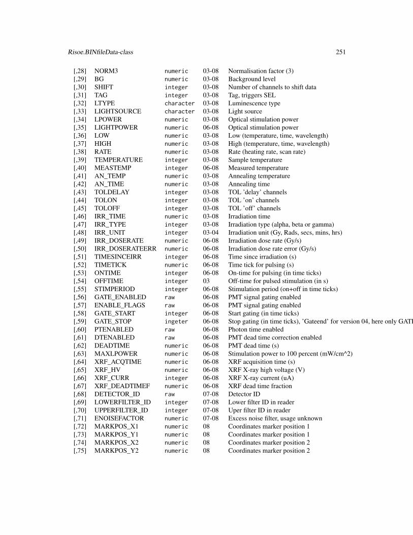
Risoe.BINfileData-class 251

[,28] NORM3 numeric 03-08 Normalisation factor (3)[,29] BG numeric 03-08 Background level[,30] SHIFT integer 03-08 Number of channels to shift data[,31] TAG integer 03-08 Tag, triggers SEL[,32] LTYPE character 03-08 Luminescence type[,33] LIGHTSOURCE character 03-08 Light source[,34] LPOWER numeric 03-08 Optical stimulation power[,35] LIGHTPOWER numeric 06-08 Optical stimulation power[,36] LOW numeric 03-08 Low (temperature, time, wavelength)[,37] HIGH numeric 03-08 High (temperature, time, wavelength)[,38] RATE numeric 03-08 Rate (heating rate, scan rate)[,39] TEMPERATURE integer 03-08 Sample temperature[,40] MEASTEMP integer 06-08 Measured temperature[,41] AN_TEMP numeric 03-08 Annealing temperature[,42] AN_TIME numeric 03-08 Annealing time[,43] TOLDELAY integer 03-08 TOL ’delay’ channels[,44] TOLON integer 03-08 TOL ’on’ channels[,45] TOLOFF integer 03-08 TOL ’off’ channels[,46] IRR_TIME numeric 03-08 Irradiation time[,47] IRR_TYPE integer 03-08 Irradiation type (alpha, beta or gamma)[,48] IRR_UNIT integer 03-04 Irradiation unit (Gy, Rads, secs, mins, hrs)[,49] IRR_DOSERATE numeric 06-08 Irradiation dose rate (Gy/s)[,50] IRR_DOSERATEERR numeric 06-08 Irradiation dose rate error (Gy/s)[,51] TIMESINCEIRR integer 06-08 Time since irradiation (s)[,52] TIMETICK numeric 06-08 Time tick for pulsing (s)[,53] ONTIME integer 06-08 On-time for pulsing (in time ticks)[,54] OFFTIME integer 03 Off-time for pulsed stimulation (in s)[,55] STIMPERIOD integer 06-08 Stimulation period (on+off in time ticks)[,56] GATE_ENABLED raw 06-08 PMT signal gating enabled[,57] ENABLE_FLAGS raw 06-08 PMT signal gating enabled[,58] GATE_START integer 06-08 Start gating (in time ticks)[,59] GATE_STOP ingeter 06-08 Stop gating (in time ticks), ’Gateend’ for version 04, here only GATE_STOP is used[,60] PTENABLED raw 06-08 Photon time enabled[,61] DTENABLED raw 06-08 PMT dead time correction enabled[,62] DEADTIME numeric 06-08 PMT dead time (s)[,63] MAXLPOWER numeric 06-08 Stimulation power to 100 percent (mW/cm^2)[,64] XRF_ACQTIME numeric 06-08 XRF acquisition time (s)[,65] XRF_HV numeric 06-08 XRF X-ray high voltage (V)[,66] XRF_CURR integer 06-08 XRF X-ray current (uA)[,67] XRF_DEADTIMEF numeric 06-08 XRF dead time fraction[,68] DETECTOR_ID raw 07-08 Detector ID[,69] LOWERFILTER_ID integer 07-08 Lower filter ID in reader[,70] UPPERFILTER_ID integer 07-08 Uper filter ID in reader[,71] ENOISEFACTOR numeric 07-08 Excess noise filter, usage unknown[,72] MARKPOS_X1 numeric 08 Coordinates marker position 1[,73] MARKPOS_Y1 numeric 08 Coordinates marker position 1[,74] MARKPOS_X2 numeric 08 Coordinates marker position 2[,75] MARKPOS_Y2 numeric 08 Coordinates marker position 2

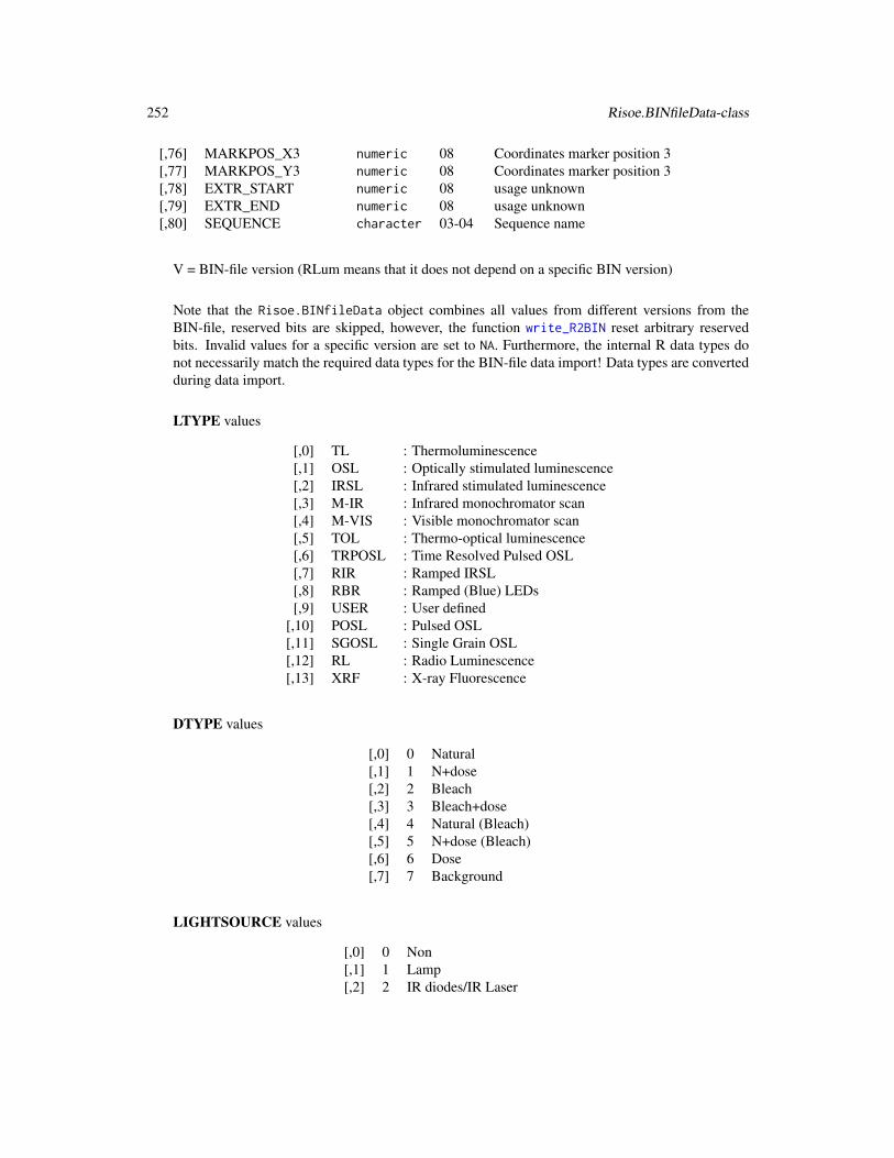
252 Risoe.BINfileData-class

[,76] MARKPOS_X3 numeric 08 Coordinates marker position 3[,77] MARKPOS_Y3 numeric 08 Coordinates marker position 3[,78] EXTR_START numeric 08 usage unknown[,79] EXTR_END numeric 08 usage unknown[,80] SEQUENCE character 03-04 Sequence name

V = BIN-file version (RLum means that it does not depend on a specific BIN version)

Note that the Risoe.BINfileData object combines all values from different versions from theBIN-file, reserved bits are skipped, however, the function write_R2BIN reset arbitrary reservedbits. Invalid values for a specific version are set to NA. Furthermore, the internal R data types donot necessarily match the required data types for the BIN-file data import! Data types are convertedduring data import.

LTYPE values

[,0] TL : Thermoluminescence[,1] OSL : Optically stimulated luminescence[,2] IRSL : Infrared stimulated luminescence[,3] M-IR : Infrared monochromator scan[,4] M-VIS : Visible monochromator scan[,5] TOL : Thermo-optical luminescence[,6] TRPOSL : Time Resolved Pulsed OSL[,7] RIR : Ramped IRSL[,8] RBR : Ramped (Blue) LEDs[,9] USER : User defined

[,10] POSL : Pulsed OSL[,11] SGOSL : Single Grain OSL[,12] RL : Radio Luminescence[,13] XRF : X-ray Fluorescence

DTYPE values

[,0] 0 Natural[,1] 1 N+dose[,2] 2 Bleach[,3] 3 Bleach+dose[,4] 4 Natural (Bleach)[,5] 5 N+dose (Bleach)[,6] 6 Dose[,7] 7 Background

LIGHTSOURCE values

[,0] 0 Non[,1] 1 Lamp[,2] 2 IR diodes/IR Laser

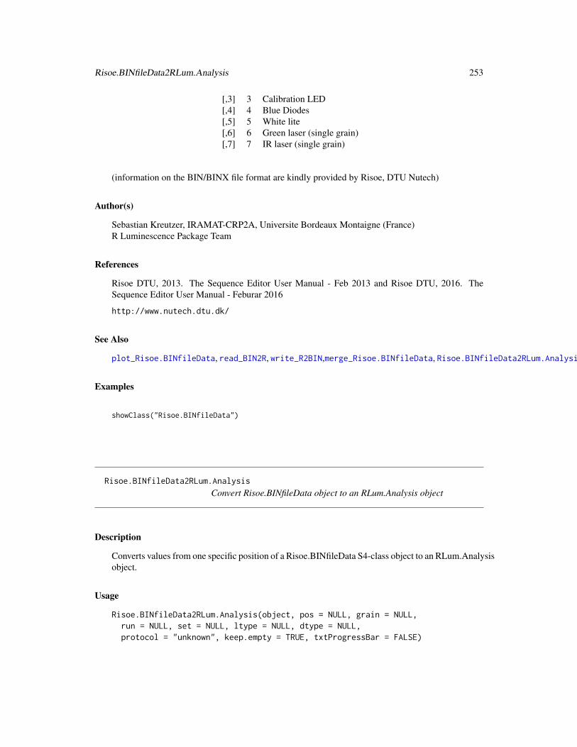
Risoe.BINfileData2RLum.Analysis 253

[,3] 3 Calibration LED[,4] 4 Blue Diodes[,5] 5 White lite[,6] 6 Green laser (single grain)[,7] 7 IR laser (single grain)

(information on the BIN/BINX file format are kindly provided by Risoe, DTU Nutech)

Author(s)


References

Risoe DTU, 2013. The Sequence Editor User Manual - Feb 2013 and Risoe DTU, 2016. TheSequence Editor User Manual - Feburar 2016

http://www.nutech.dtu.dk/

See Also

plot_Risoe.BINfileData, read_BIN2R, write_R2BIN,merge_Risoe.BINfileData, Risoe.BINfileData2RLum.Analysis,

Examples

showClass("Risoe.BINfileData")

Risoe.BINfileData2RLum.Analysis

Convert Risoe.BINfileData object to an RLum.Analysis object

Description

Converts values from one specific position of a Risoe.BINfileData S4-class object to an RLum.Analysisobject.

Usage

Risoe.BINfileData2RLum.Analysis(object, pos = NULL, grain = NULL,run = NULL, set = NULL, ltype = NULL, dtype = NULL,protocol = "unknown", keep.empty = TRUE, txtProgressBar = FALSE)

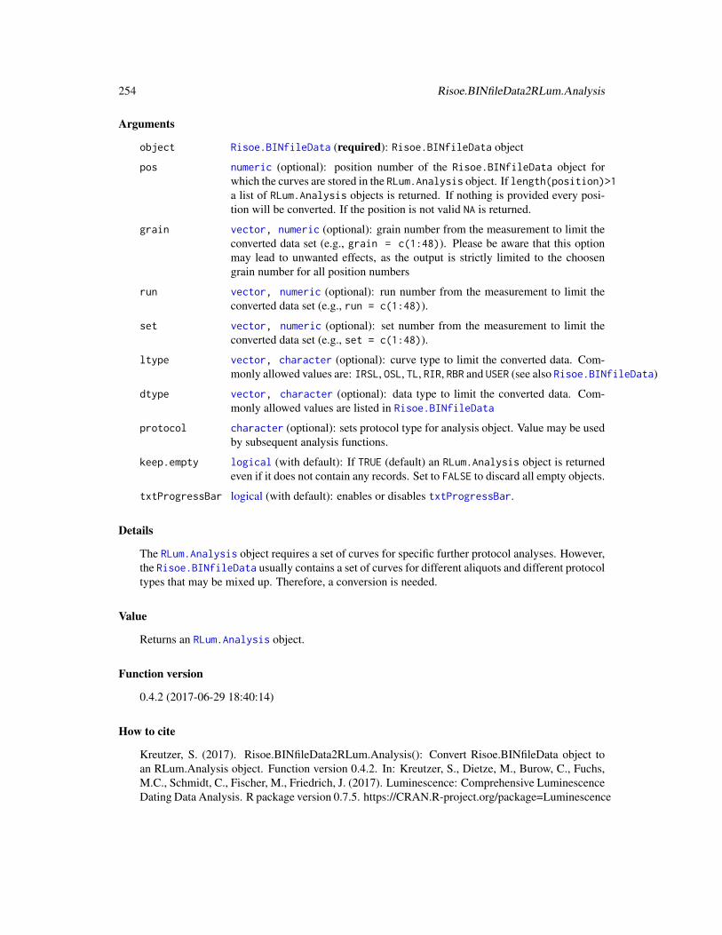
254 Risoe.BINfileData2RLum.Analysis

Arguments

object Risoe.BINfileData (required): Risoe.BINfileData object

pos numeric (optional): position number of the Risoe.BINfileData object forwhich the curves are stored in the RLum.Analysis object. If length(position)>1a list of RLum.Analysis objects is returned. If nothing is provided every posi-tion will be converted. If the position is not valid NA is returned.

grain vector, numeric (optional): grain number from the measurement to limit theconverted data set (e.g., grain = c(1:48)). Please be aware that this optionmay lead to unwanted effects, as the output is strictly limited to the choosengrain number for all position numbers

run vector, numeric (optional): run number from the measurement to limit theconverted data set (e.g., run = c(1:48)).

set vector, numeric (optional): set number from the measurement to limit theconverted data set (e.g., set = c(1:48)).

ltype vector, character (optional): curve type to limit the converted data. Com-monly allowed values are: IRSL, OSL, TL, RIR, RBR and USER (see also Risoe.BINfileData)

dtype vector, character (optional): data type to limit the converted data. Com-monly allowed values are listed in Risoe.BINfileData

protocol character (optional): sets protocol type for analysis object. Value may be usedby subsequent analysis functions.

keep.empty logical (with default): If TRUE (default) an RLum.Analysis object is returnedeven if it does not contain any records. Set to FALSE to discard all empty objects.


Details

The RLum.Analysis object requires a set of curves for specific further protocol analyses. However,the Risoe.BINfileData usually contains a set of curves for different aliquots and different protocoltypes that may be mixed up. Therefore, a conversion is needed.

Value

Returns an RLum.Analysis object.

Function version

0.4.2 (2017-06-29 18:40:14)

How to cite

Kreutzer, S. (2017). Risoe.BINfileData2RLum.Analysis(): Convert Risoe.BINfileData object toan RLum.Analysis object. Function version 0.4.2. In: Kreutzer, S., Dietze, M., Burow, C., Fuchs,M.C., Schmidt, C., Fischer, M., Friedrich, J. (2017). Luminescence: Comprehensive LuminescenceDating Data Analysis. R package version 0.7.5. https://CRAN.R-project.org/package=Luminescence

RLum-class 255

Note

The protocol argument of the RLum.Analysis object is set to ’unknown’ if not stated otherwise.

Author(s)


References

#

See Also

Risoe.BINfileData, RLum.Analysis, read_BIN2R

Examples


##convert values for position 1Risoe.BINfileData2RLum.Analysis(CWOSL.SAR.Data, pos = 1)

RLum-class Class "RLum"

Description

Abstract class for data in the package Luminescence

Usage

## S4 method for signature 'RLum'replicate_RLum(object, times = NULL)

Arguments

object an object of class RLum (required)

times integer (optional): number for times each element is repeated element


• replicate_RLum: Replication method RLum-objects

256 RLum-class

Slots

originator Object of class character containing the name of the producing function for theobject. Set automatically by using the function set_RLum.

info Object of class list for additional information on the object itself

.uid Object of class character for a unique object identifier. This id is usually calculated usingthe internal function .create_UID() if the funtion set_RLum is called.

.pid Object of class character for a parent id. This allows nesting RLum-objects at will. Theparent id can be the uid of another object.


A virtual Class: No objects can be created from it.

Class version

0.4.0

How to cite

Kreutzer, S. (2017). RLum-class(): Class ’RLum’. In: Kreutzer, S., Dietze, M., Burow, C., Fuchs,M.C., Schmidt, C., Fischer, M., Friedrich, J. (2017). Luminescence: Comprehensive LuminescenceDating Data Analysis. R package version 0.7.5. https://CRAN.R-project.org/package=Luminescence

Note

RLum is a virtual class.

Author(s)


See Also

RLum.Data, RLum.Analysis

Examples

showClass("RLum")

RLum.Analysis-class 257

RLum.Analysis-class Class "RLum.Analysis"

Description

Object class to represent analysis data for protocol analysis, i.e. all curves, spectra etc. from onemeasurements. Objects from this class are produced, by e.g. read_XSYG2R, read_Daybreak2R

Usage

## S4 method for signature 'RLum.Analysis'show(object)

## S4 method for signature 'RLum.Analysis'set_RLum(class, originator, .uid, .pid,protocol = NA_character_, records = list(), info = list())

## S4 method for signature 'RLum.Analysis'get_RLum(object, record.id = NULL,recordType = NULL, curveType = NULL, RLum.type = NULL,protocol = "UNKNOWN", get.index = NULL, drop = TRUE, recursive = TRUE,info.object = NULL, subset = NULL)

## S4 method for signature 'RLum.Analysis'structure_RLum(object, fullExtent = FALSE)

## S4 method for signature 'RLum.Analysis'length_RLum(object)

## S4 method for signature 'RLum.Analysis'names_RLum(object)

## S4 method for signature 'RLum.Analysis'smooth_RLum(object, ...)

Arguments

object [show_RLum][get_RLum][names_RLum][length_RLum] [structure_RLum]] anobject of class RLum.Analysis (required)

class [set_RLum] character (required): name of the RLum class to be created

originator [set_RLum] character (automatic): contains the name of the calling function(the function that produces this object); can be set manually.

.uid [set_RLum] character (automatic): sets an unique ID for this object using theinternal C++ function .create_UID.

.pid [set_RLum] character (with default): option to provide a parent id for nestingat will.

258 RLum.Analysis-class

protocol [set_RLum] character (optional): sets protocol type for analysis object. Valuemay be used by subsequent analysis functions.

records [set_RLum] list (required): list of RLum.Analysis objects

info [set_RLum] list (optional): a list containing additional info data for the objectset_RLum:

Returns an RLum.Analysis object.

record.id [get_RLum] numeric or logical (optional): IDs of specific records. If of typelogical the entire id range is assuemd and TRUE and FALSE indicates the selec-tion.

recordType [get_RLum] character (optional): record type (e.g., "OSL"). Can be also avector, for multiple matching, e.g., recordType = c("OSL", "IRSL")

curveType [get_RLum] character (optional): curve type (e.g. "predefined" or "measured")

RLum.type [get_RLum] character (optional): RLum object type. Defaults to "RLum.Data.Curve"and "RLum.Data.Spectrum".

get.index [get_RLum] logical (optional): return a numeric vector with the index of eachelement in the RLum.Analysis object.

drop [get_RLum] logical (with default): coerce to the next possible layer (which areRLum.Data-objects), drop = FALSE keeps the original RLum.Analysis

recursive [get_RLum] logical (with default): if TRUE (the default) and the result of the’get_RLum’ request is a single object this object will be unlisted, means onlythe object itself and no list containing exactly one object is returned. Mostlythis makes things easier, however, if this method is used within a loop this mightundesired.

info.object [get_RLum] character (optional): name of the wanted info element

subset expression (optional): logical expression indicating elements or rows to keep:missing values are taken as false. This argument takes precedence over all otherarguments, meaning they are not considered when subsetting the object.

fullExtent [structure_RLum] logical (with default): extents the returned data.frame toits full extent, i.e. all info elements are part of the return as well. The defaultvalule is FALSE as the data frame might become rather big.

... further arguments passed to underlying methods

Value

get_RLum:

Returns:(1) list of RLum.Data objects or(2) Single RLum.Data object, if only one object is contained and recursive = FALSE or(3) RLum.Analysis ojects for drop = FALSE

structure_RLum:

RLum.Analysis-class 259

Returns data.frame showing the structure.

length_RLum

Returns the number records in this object.

names_RLum

Returns the names of the record types (recordType) in this object.

smooth_RLum

Same object as input, after smoothing


• show: Show structure of RLum.Analysis object

• set_RLum: Construction method for RLum.Analysis objects.

• get_RLum: Accessor method for RLum.Analysis object.The slots record.id, recordType, curveType and RLum.type are optional to allow for recordslimited by their id (list index number), their record type (e.g. recordType = "OSL") or objecttype.Example: curve type (e.g. curveType = "predefined" or curveType ="measured")The selection of a specific RLum.type object superimposes the default selection. Currentlysupported objects are: RLum.Data.Curve and RLum.Data.Spectrum

• structure_RLum: Method to show the structure of an RLum.Analysis object.

• length_RLum: Returns the length of the object, i.e., number of stored records.

• names_RLum: Returns the names of the RLum.Data objects objects (same as shown with theshow method)

• smooth_RLum: Smoothing of RLum.Data objects contained in this RLum.Analysis objectrollmean or rollmedian. In particular the internal function .smoothing is used.

Slots

protocol Object of class character describing the applied measurement protocol

records Object of class list containing objects of class RLum.Data


Objects can be created by calls of the form set_RLum("RLum.Analysis", ...).

Class version

0.4.8

260 RLum.Data-class

How to cite

Kreutzer, S. (2017). RLum.Analysis-class(): Class ’RLum.Analysis’. In: Kreutzer, S., Dietze, M.,Burow, C., Fuchs, M.C., Schmidt, C., Fischer, M., Friedrich, J. (2017). Luminescence: Comprehen-sive Luminescence Dating Data Analysis. R package version 0.7.5. https://CRAN.R-project.org/package=Luminescence

Note

The method structure_RLum is currently just avaiblable for objects containing RLum.Data.Curve.

Author(s)


See Also

Risoe.BINfileData2RLum.Analysis, Risoe.BINfileData, RLum

Examples

showClass("RLum.Analysis")

##set empty objectset_RLum(class = "RLum.Analysis")

###use example data##load datadata(ExampleData.RLum.Analysis, envir = environment())

##show curves in objectget_RLum(IRSAR.RF.Data)

##show only the first object, but by keeping the objectget_RLum(IRSAR.RF.Data, record.id = 1, drop = FALSE)

RLum.Data-class Class "RLum.Data"

Description

Generalized virtual data class for luminescence data.


A virtual Class: No objects can be created from it.

Class version

0.2.1

RLum.Data.Curve-class 261

Note

Just a virtual class.

Author(s)


See Also

RLum, RLum.Data.Curve, RLum.Data.Spectrum

Examples

showClass("RLum.Data")

RLum.Data.Curve-class Class "RLum.Data.Curve"

Description

Class for representing luminescence curve data.

Usage

## S4 method for signature 'RLum.Data.Curve'show(object)

## S4 method for signature 'RLum.Data.Curve'set_RLum(class, originator, .uid, .pid,recordType = NA_character_, curveType = NA_character_, data = matrix(0,ncol = 2), info = list())

## S4 method for signature 'RLum.Data.Curve'get_RLum(object, info.object = NULL)

## S4 method for signature 'RLum.Data.Curve'length_RLum(object)

## S4 method for signature 'RLum.Data.Curve'names_RLum(object)

## S4 method for signature 'RLum.Data.Curve'bin_RLum.Data(object, bin_size = 2)

## S4 method for signature 'RLum.Data.Curve'smooth_RLum(object, k = NULL, fill = NA,align = "right", method = "mean")

262 RLum.Data.Curve-class

Arguments

object [show_RLum][get_RLum][length_RLum][names_RLum] an object of class RLum.Data.Curve(required)

class [set_RLum] character (required): name of the RLum class to create

originator [set_RLum] character (automatic): contains the name of the calling function(the function that produces this object); can be set manually.



recordType [set_RLum] character (optional): record type (e.g., "OSL")

curveType [set_RLum] character (optional): curve type (e.g., "predefined" or "measured")

data [set_RLum] matrix (required): raw curve data. If data itself is a RLum.Data.Curve-object this can be used to re-construct the object (s. Details)

info [set_RLum] list (optional): info elements

info.object [get_RLum] character (optional): name of the wanted info element

bin_size [bin_RLum] integer (with default): set number of channels used for each bin,e.g. bin_size = 2 means that two channels are binned.

k [smooth_RLum] integer (with default): window for the rolling mean; must beodd for rollmedian. If nothing is set k is set automatically

fill [smooth_RLum] numeric (with default): a vector defining the left and the righthand data

align [smooth_RLum] character (with default): specifying whether the index of theresult should be left- or right-aligned or centered (default) compared to therolling window of observations, allowed "right", "center" and left

method [smooth_RLum] character (with default): defines which method should be ap-plied for the smoothing: "mean" or "median"

Value

set_RLum

Returns an RLum.Data.Curve object.

get_RLum

(1) A matrix with the curve values or(2) only the info object if info.object was set.

length_RLum

Number of channels in the curve (row number of the matrix)

RLum.Data.Curve-class 263

names_RLum

Names of the info elements (slot info)

bin_RLum.Data

Same object as input, after applying the binning.

smooth_RLum

Same object as input, after smoothing


• show: Show structure of RLum.Data.Curve object

• set_RLum: Construction method for RLum.Data.Curve object. The slot info is optional andpredefined as empty list by default.

• get_RLum: Accessor method for RLum.Data.Curve object. The argument info.object is op-tional to directly access the info elements. If no info element name is provided, the raw curvedata (matrix) will be returned.

• length_RLum: Returns the length of the curve object, which is the maximum of the valuetime/temperature of the curve (corresponding to the stimulation length)

• names_RLum: Returns the names info elements coming along with this curve object

• bin_RLum.Data: Allows binning of specific objects

• smooth_RLum: Smoothing of RLum.Data.Curve objects using the function rollmean or rollmedian.In particular the internal function .smoothing is used.

Slots

recordType Object of class "character" containing the type of the curve (e.g. "TL" or "OSL")

curveType Object of class "character" containing curve type, allowed values are measured or pre-defined

data Object of class matrix containing curve x and y data. ’data’ can also be of type RLum.Data.Curveto change object values without deconstructing the object. For example: set_RLum(class = 'RLum.Data.Curve',data = Your.RLum.Data.Curve, recordType = 'never seen before')would just change the recordType. Missing arguements the value is taken from the input objectin ’data’ (which is already an RLum.Data.Curve object in this example)

Create objects from this Class

Objects can be created by calls of the form set_RLum(class = "RLum.Data.Curve", ...).

Class version

0.5.0

264 RLum.Data.Image-class

How to cite

Kreutzer, S. (2017). RLum.Data.Curve-class(): Class ’RLum.Data.Curve’. In: Kreutzer, S., Di-etze, M., Burow, C., Fuchs, M.C., Schmidt, C., Fischer, M., Friedrich, J. (2017). Luminescence:Comprehensive Luminescence Dating Data Analysis. R package version 0.7.5. https://CRAN.R-project.org/package=Luminescence

Note

The class should only contain data for a single curve. For additional elements the slot info can beused (e.g. providing additional heating ramp curve). Objects from the class RLum.Data.Curve areproduced by other functions (partyl within RLum.Analysis objects), namely: Risoe.BINfileData2RLum.Analysis,read_XSYG2R

Author(s)


See Also

RLum, RLum.Data, plot_RLum, merge_RLum

Examples

showClass("RLum.Data.Curve")

##set empty curve objectset_RLum(class = "RLum.Data.Curve")

RLum.Data.Image-class Class "RLum.Data.Image"

Description

Class for representing luminescence image data (TL/OSL/RF). Such data are for example producedby the function read_SPE2R

Usage

## S4 method for signature 'RLum.Data.Image'show(object)

## S4 method for signature 'RLum.Data.Image'set_RLum(class, originator, .uid, .pid,recordType = "Image", curveType = NA_character_,data = raster::brick(raster::raster(matrix())), info = list())

RLum.Data.Image-class 265

## S4 method for signature 'RLum.Data.Image'get_RLum(object, info.object)

## S4 method for signature 'RLum.Data.Image'names_RLum(object)

Arguments

object [show_RLum][get_RLum][names_RLum] an object of class RLum.Data.Imageclass [set_RLum]character: name of the RLum class to createoriginator [set_RLum] character (automatic): contains the name of the calling function

(the function that produces this object); can be set manually..uid [set_RLum] character (automatic): sets an unique ID for this object using the

internal C++ function .create_UID..pid [set_RLum] character (with default): option to provide a parent id for nesting

at will.recordType [set_RLum] character: record type (e.g. "OSL")curveType [set_RLum] character: curve type (e.g. "predefined" or "measured")data [set_RLum] matrix: raw curve data. If data is of type RLum.Data.Image this

can be used to re-construct the object.info [set_RLum] list: info elementsinfo.object [get_RLum] character name of the info object to returned

Value

set_RLum

Returns an object from class RLum.Data.Image

get_RLum

(1) Returns the data object (brick)(2) only the info object if info.object was set.

names_RLum

Returns the names of the info elements


• show: Show structure of RLum.Data.Image object• set_RLum: Construction method for RLum.Data.Image object. The slot info is optional and

predefined as empty list by default..• get_RLum: Accessor method for RLum.Data.Image object. The argument info.object is op-

tional to directly access the info elements. If no info element name is provided, the raw imagedata (RasterBrick) will be returned.


266 RLum.Data.Image-class

Slots

recordType Object of class character containing the type of the curve (e.g. "OSL image", "TLimage")

curveType Object of class character containing curve type, allowed values are measured or pre-defined

data Object of class brick containing images (raster data).

info Object of class list containing further meta information objects


Objects can be created by calls of the form set_RLum("RLum.Data.Image", ...).

Class version

0.4.0

How to cite

Kreutzer, S. (2017). RLum.Data.Image-class(): Class ’RLum.Data.Image’. In: Kreutzer, S., Di-etze, M., Burow, C., Fuchs, M.C., Schmidt, C., Fischer, M., Friedrich, J. (2017). Luminescence:Comprehensive Luminescence Dating Data Analysis. R package version 0.7.5. https://CRAN.R-project.org/package=Luminescence

Note

The class should only contain data for a set of images. For additional elements the slot info can beused.

Author(s)


See Also

RLum, RLum.Data, plot_RLum, read_SPE2R

Examples

showClass("RLum.Data.Image")

##create empty RLum.Data.Image objectset_RLum(class = "RLum.Data.Image")

RLum.Data.Spectrum-class 267

RLum.Data.Spectrum-class

Class "RLum.Data.Spectrum"

Description

Class for representing luminescence spectra data (TL/OSL/RF).

Usage

## S4 method for signature 'RLum.Data.Spectrum'show(object)

## S4 method for signature 'RLum.Data.Spectrum'set_RLum(class, originator, .uid, .pid,recordType = "Spectrum", curveType = NA_character_, data = matrix(),info = list())

## S4 method for signature 'RLum.Data.Spectrum'get_RLum(object, info.object)

## S4 method for signature 'RLum.Data.Spectrum'names_RLum(object)

Arguments

object [show_RLum][get_RLum][names_RLum] an object of class RLum.Data.Spectrum

class [set_RLum] character (automatic): name of the RLum class to create.

originator character (automatic): contains the name of the calling function (the functionthat produces this object); can be set manually.



recordType [set_RLum] character: record type (e.g. "OSL")

curveType [set_RLum] character: curve type (e.g. "predefined" or "measured")

data [set_RLum] matrix: raw curve data. If data is of type RLum.Data.Spectrum,this can be used to re-construct the object.

info [set_RLum] list: info elements

info.object [get_RLum] character (optional): the name of the info object to be called

268 RLum.Data.Spectrum-class

Value

[set_RLum]

An object from the class RLum.Data.Spectrum

get_RLum

(1) A matrix with the spectrum values or(2) only the info object if info.object was set.

names_RLum

The names of the info objects


• show: Show structure of RLum.Data.Spectrum object

• set_RLum: Construction method for RLum.Data.Spectrum object. The slot info is optionaland predefined as empty list by default

• get_RLum: Accessor method for RLum.Data.Spectrum object. The argument info.object isoptional to directly access the info elements. If no info element name is provided, the rawcurve data (matrix) will be returned


Slots

recordType Object of class character containing the type of the curve (e.g. "TL" or "OSL")

curveType Object of class character containing curve type, allowed values are measured or pre-defined

data Object of class matrix containing spectrum (count) values. Row labels indicate wave-length/pixel values, column labels are temperature or time values.

info Object of class list containing further meta information objects


Objects can be created by calls of the form set_RLum("RLum.Data.Spectrum", ...).

Class version

0.4.0

How to cite

Kreutzer, S. (2017). RLum.Data.Spectrum-class(): Class ’RLum.Data.Spectrum’. In: Kreutzer, S.,Dietze, M., Burow, C., Fuchs, M.C., Schmidt, C., Fischer, M., Friedrich, J. (2017). Luminescence:Comprehensive Luminescence Dating Data Analysis. R package version 0.7.5. https://CRAN.R-project.org/package=Luminescence

RLum.Results-class 269

Note

The class should only contain data for a single spectra data set. For additional elements the slotinfo can be used. Objects from this class are automatically created by, e.g., read_XSYG2R

Author(s)


See Also

RLum, RLum.Data, plot_RLum

Examples

showClass("RLum.Data.Spectrum")

##show example datadata(ExampleData.XSYG, envir = environment())TL.Spectrum

##show data matrixget_RLum(TL.Spectrum)

##plot spectrum## Not run:plot_RLum(TL.Spectrum)

## End(Not run)

RLum.Results-class Class "RLum.Results"

Description

Object class contains results data from functions (e.g., analyse_SAR.CWOSL).

Usage

## S4 method for signature 'RLum.Results'show(object)

## S4 method for signature 'RLum.Results'set_RLum(class, originator, .uid, .pid,data = list(), info = list())

## S4 method for signature 'RLum.Results'get_RLum(object, data.object, info.object = NULL,

270 RLum.Results-class

drop = TRUE)

## S4 method for signature 'RLum.Results'length_RLum(object)

## S4 method for signature 'RLum.Results'names_RLum(object)

Arguments

object [get_RLum] RLum.Results (required): an object of class RLum.Results to beevaluated

class [set_RLum] character (required): name of the RLum class to createoriginator [set_RLum] character (automatic): contains the name of the calling function

(the function that produces this object); can be set manually..uid [set_RLum] character (automatic): sets an unique ID for this object using the

internal C++ function .create_UID..pid [set_RLum] character (with default): option to provide a parent id for nesting

at will.data [set_RLum] list (optional): a list containing the data to be stored in the objectinfo [set_RLum] list (optional): a list containing additional info data for the objectdata.object [get_RLum] character or numeric: name or index of the data slot to be returnedinfo.object [get_RLum] character (optional): name of the wanted info elementdrop [get_RLum] logical (with default): coerce to the next possible layer (which are

data objects, drop = FALSE keeps the original RLum.Results

Value

set_RLum:

Returns an object from the class RLum.Results

get_RLum:

Returns:(1) Data object from the specified slot(2) list of data objects from the slots if ’data.object’ is vector or(3) an RLum.Results for drop = FALSE.

length_RLum

Returns the number of data elements in the RLum.Results object.

names_RLum

Returns the names of the data elements in the object.

RLum.Results-class 271


• show: Show structure of RLum.Results object

• set_RLum: Construction method for an RLum.Results object.

• get_RLum: Accessor method for RLum.Results object. The argument data.object allows di-rectly accessing objects delivered within the slot data. The default return object depends onthe object originator (e.g., fit_LMCurve). If nothing is specified always the first data.objectwill be returned.

Note: Detailed specification should be made in combination with the originator slot in thereceiving function if results are pipped.

• length_RLum: Returns the length of the object, i.e., number of stored data.objects

• names_RLum: Returns the names data.objects

Slots

data Object of class "list" containing output data


Objects can be created by calls of the form new("RLum.Results", ...).

Class version

0.5.1

How to cite

Kreutzer, S. (2017). RLum.Results-class(): Class ’RLum.Results’. In: Kreutzer, S., Dietze, M.,Burow, C., Fuchs, M.C., Schmidt, C., Fischer, M., Friedrich, J. (2017). Luminescence: Comprehen-sive Luminescence Dating Data Analysis. R package version 0.7.5. https://CRAN.R-project.org/package=Luminescence

Note

The class is intended to store results from functions to be used by other functions. The data in theobject should always be accessed by the method get_RLum.

Author(s)


See Also

RLum, plot_RLum, merge_RLum

272 Second2Gray

Examples

showClass("RLum.Results")

##create an empty object from this classset_RLum(class = "RLum.Results")

##use another function to show how it works

##Basic calculation of the dose rate for a specific datedose.rate <- calc_SourceDoseRate(measurement.date = "2012-01-27",calib.date = "2014-12-19",calib.dose.rate = 0.0438,calib.error = 0.0019)

##show objectdose.rate

##get resultsget_RLum(dose.rate)

##get parameters used for the calcualtion from the same objectget_RLum(dose.rate, data.object = "parameters")

##alternatively objects can be accessed using S3 generics, such asdose.rate$parameters

Second2Gray Converting equivalent dose values from seconds (s) to gray (Gy)

Description

Conversion of absorbed radiation dose in seconds (s) to the SI unit gray (Gy) including error prop-agation. Normally used for equivalent dose data.

Usage

Second2Gray(data, dose.rate, error.propagation = "omit")

Arguments

data data.frame (required): input values, structure: data (values[,1]) and dataerror (values [,2]) are required

dose.rate RLum.Results or data.frame or numeric (required): RLum.Results needs tobe orginated from the function calc_SourceDoseRate, for vector dose rate inGy/s and dose rate error in Gy/s

Second2Gray 273

error.propagation

character (with default): error propagation method used for error calculation(omit, gaussian or absolute), see details for further information

Details

Calculation of De values from seconds (s) to gray (Gy)

De[Gy] = De[s] ∗DoseRate[Gy/s])

Provided calculation error propagation methods for error calculation (with ’se’ as the standard errorand ’DR’ of the dose rate of the beta-source):

(1) omit (default)

se(De)[Gy] = se(De)[s] ∗DR[Gy/s]

In this case the standard error of the dose rate of the beta-source is treated as systematic (i.e. non-random), it error propagation is omitted. However, the error must be considered during calculationof the final age. (cf. Aitken, 1985, pp. 242). This approach can be seen as method (2) (gaussian) forthe case the (random) standard error of the beta-source calibration is 0. Which particular method isrequested depends on the situation and cannot be prescriptive.

(2) gaussian error propagation

se(De)[Gy] =√

((DR[Gy/s] ∗ se(De)[s])2 + (De[s] ∗ se(DR)[Gy/s])2)

Applicable under the assumption that errors of De and se are uncorrelated.

(3) absolute error propagation

se(De)[Gy] = abs(DR[Gy/s] ∗ se(De)[s]) + abs(De[s] ∗ se(DR)[Gy/s])

Applicable under the assumption that errors of De and se are not uncorrelated.

Value

Returns a data.frame with converted values.

Function version

0.6.0 (2017-06-29 18:40:14)

274 Second2Gray

How to cite

Kreutzer, S., Dietze, M., Fuchs, M.C., Fuchs, M. (2017). Second2Gray(): Converting equiva-lent dose values from seconds (s) to gray (Gy). Function version 0.6.0. In: Kreutzer, S., Di-etze, M., Burow, C., Fuchs, M.C., Schmidt, C., Fischer, M., Friedrich, J. (2017). Luminescence:Comprehensive Luminescence Dating Data Analysis. R package version 0.7.5. https://CRAN.R-project.org/package=Luminescence

Note

If no or a wrong error propagation method is given, the execution of the function is stopped. Fur-thermore, if a data.frame is provided for the dose rate values is has to be of the same length as thedata frame provided with the argument data

Author(s)

Sebastian Kreutzer, IRAMAT-CRP2A, Universite Bordeaux Montaigne (France),Michael Dietze, GFZ Potsdam (Germany),Margret C. Fuchs, HZDR, Helmholtz-Institute Freiberg for Resource Technology (Germany)R Luminescence Package Team

References

Aitken, M.J., 1985. Thermoluminescence dating. Academic Press.

See Also

calc_SourceDoseRate

Examples

##(A) for known source dose rate at date of measurement## - load De data from the example data help filedata(ExampleData.DeValues, envir = environment())## - convert De(s) to De(Gy)Second2Gray(ExampleData.DeValues$BT998, c(0.0438,0.0019))

##(B) for source dose rate calibration data## - calculate source dose rate firstdose.rate <- calc_SourceDoseRate(measurement.date = "2012-01-27",

calib.date = "2014-12-19",calib.dose.rate = 0.0438,calib.error = 0.0019)

# read example datadata(ExampleData.DeValues, envir = environment())

set_Risoe.BINfileData 275

# apply dose.rate to convert De(s) to De(Gy)Second2Gray(ExampleData.DeValues$BT998, dose.rate)

set_Risoe.BINfileData General accessor function for RLum S4 class objects

Description

Function calls object-specific get functions for RisoeBINfileData S4 class objects.

Usage

set_Risoe.BINfileData(METADATA = data.frame(), DATA = list(),.RESERVED = list())

Arguments

METADATA x

DATA x

.RESERVED x

Details

The function provides a generalised access point for specific Risoe.BINfileData objects.Depending on the input object, the corresponding get function will be selected. Allowed argumentscan be found in the documentations of the corresponding Risoe.BINfileData class.

Value


Function version

0.1 (2017-06-29 18:40:14)

How to cite

Kreutzer, S. (2017). set_Risoe.BINfileData(): General accessor function for RLum S4 class objects.Function version 0.1. In: Kreutzer, S., Dietze, M., Burow, C., Fuchs, M.C., Schmidt, C., Fischer,M., Friedrich, J. (2017). Luminescence: Comprehensive Luminescence Dating Data Analysis. Rpackage version 0.7.5. https://CRAN.R-project.org/package=Luminescence

Author(s)


276 set_RLum

See Also

Risoe.BINfileData

set_RLum General set function for RLum S4 class objects

Description

Function calls object-specific set functions for RLum S4 class objects.

Usage

set_RLum(class, originator, .uid = .create_UID(), .pid = NA_character_, ...)

Arguments

class RLum (required): name of the S4 class to create

originator character (automatic): contains the name of the calling function (the functionthat produces this object); can be set manually.

.uid character (automatic): sets an unique ID for this object using the internal C++function .create_UID.

.pid character (with default): option to provide a parent id for nesting at will.

... further arguments that one might want to pass to the specific set method

Details

The function provides a generalised access point for specific RLum objects.Depending on the given class, the corresponding method to create an object from this class will beselected. Allowed additional arguments can be found in the documentations of the correspondingRLum class: RLum.Data.Curve, RLum.Data.Image, RLum.Data.Spectrum, RLum.Analysis andRLum.Results

Value

Returns an object of the specified class.

Function version

0.3.0 (2017-06-29 18:40:14)

How to cite

Kreutzer, S. (2017). set_RLum(): General set function for RLum S4 class objects. Function version0.3.0. In: Kreutzer, S., Dietze, M., Burow, C., Fuchs, M.C., Schmidt, C., Fischer, M., Friedrich, J.(2017). Luminescence: Comprehensive Luminescence Dating Data Analysis. R package version0.7.5. https://CRAN.R-project.org/package=Luminescence

smooth_RLum 277

Author(s)


See Also


Examples

##produce empty objects from each classset_RLum(class = "RLum.Data.Curve")set_RLum(class = "RLum.Data.Spectrum")set_RLum(class = "RLum.Data.Spectrum")set_RLum(class = "RLum.Analysis")set_RLum(class = "RLum.Results")

##produce a curve object with arbitrary curve valuesobject <- set_RLum(class = "RLum.Data.Curve",curveType = "arbitrary",recordType = "OSL",data = matrix(c(1:100,exp(-c(1:100))),ncol = 2))

##plot this curve objectplot_RLum(object)

smooth_RLum Smoothing of data

Description

Function calls the object-specific smooth functions for provided RLum S4-class objects.

Usage

smooth_RLum(object, ...)

## S4 method for signature 'list'smooth_RLum(object, ...)

Arguments


... further arguments passed to the specifc class method

278 smooth_RLum

Details

The function provides a generalised access point for specific RLum objects.Depending on the input object, the corresponding function will be selected. Allowed argumentscan be found in the documentations of the corresponding RLum class. The smoothing is based on aninternal function called .smoothing.

Value

An object of the same type as the input object is provided

Methods (by class)

• list: Returns a list of RLum objects that had been passed to smooth_RLum

Function version

0.1.0 (2017-06-29 18:40:14)

How to cite

Kreutzer, S. (2017). smooth_RLum(): Smoothing of data. Function version 0.1.0. In: Kreutzer, S.,Dietze, M., Burow, C., Fuchs, M.C., Schmidt, C., Fischer, M., Friedrich, J. (2017). Luminescence:Comprehensive Luminescence Dating Data Analysis. R package version 0.7.5. https://CRAN.R-project.org/package=Luminescence

Note

Currenlty only RLum objects of class RLum.Data.Curve and RLum.Analysis (with curve data) aresupported!

Author(s)


See Also

RLum.Data.Curve, RLum.Analysis

Examples

##load example datadata(ExampleData.CW_OSL_Curve, envir = environment())

##create RLum.Data.Curve object from this examplecurve <-

set_RLum(class = "RLum.Data.Curve",recordType = "OSL",

sTeve 279

data = as.matrix(ExampleData.CW_OSL_Curve))

##plot data without and with smoothingplot_RLum(curve)plot_RLum(smooth_RLum(curve))

sTeve sTeve - sophisticated tool for efficient data validation and evaluation

Description

This function provides a sophisticated routine for comprehensive luminescence dating data analysis.

Usage

sTeve(n_frames = 10, t_animation = 2, n.tree = 7, type)

Arguments

n_frames integer (with default): n frames

t_animation integer (with default): t animation

n.tree integer (with default): How many trees do you want to cut?

type integer (optional): Make a decision: 1, 2 or 3

Details

This amazing sophisticated function validates your data seriously.

Value

Validates your data.

How to cite

NA, NA, , (2017). sTeve(): sTeve - sophisticated tool for efficient data validation and evaluation.In: Kreutzer, S., Dietze, M., Burow, C., Fuchs, M.C., Schmidt, C., Fischer, M., Friedrich, J. (2017).Luminescence: Comprehensive Luminescence Dating Data Analysis. R package version 0.7.5.https://CRAN.R-project.org/package=Luminescence

Note

This function should not be taken too seriously.

Author(s)

R Luminescence Team, 2012-2013

280 structure_RLum

References

#

See Also

plot_KDE

Examples

##no example available

structure_RLum General structure function for RLum S4 class objects

Description


Usage

structure_RLum(object, ...)

Arguments

object RLum (required): S4 object of class RLum... further arguments that one might want to pass to the specific structure method

Details

The function provides a generalised access point for specific RLum objects.Depending on the input object, the corresponding structure function will be selected. Allowedarguments can be found in the documentations of the corresponding RLum class.

Value

Returns a data.frame with structure of the object.

Function version

0.2.0 (2017-06-29 18:40:14)

How to cite

Kreutzer, S. (2017). structure_RLum(): General structure function for RLum S4 class objects.Function version 0.2.0. In: Kreutzer, S., Dietze, M., Burow, C., Fuchs, M.C., Schmidt, C., Fischer,M., Friedrich, J. (2017). Luminescence: Comprehensive Luminescence Dating Data Analysis. Rpackage version 0.7.5. https://CRAN.R-project.org/package=Luminescence

template_DRAC 281

Author(s)


See Also


Examples


##show structurestructure_RLum(OSL.SARMeasurement$Sequence.Object)

template_DRAC Create a DRAC input data template (v1.1)

Description

This function returns a DRAC input template (v1.1) to be used in conjunction with the use_DRAC()function

Usage

template_DRAC(nrow = 1, notification = TRUE)

Arguments

nrow integer (with default): specifies the number of rows of the template (i.e., thenumber of data sets you want to submit)

notification logical (with default): show or hide the notification

Value

A list.

How to cite

Burow, C. (2017). template_DRAC(): Create a DRAC input data template (v1.1). In: Kreutzer, S.,Dietze, M., Burow, C., Fuchs, M.C., Schmidt, C., Fischer, M., Friedrich, J. (2017). Luminescence:Comprehensive Luminescence Dating Data Analysis. R package version 0.7.5. https://CRAN.R-project.org/package=Luminescence

282 template_DRAC

Author(s)


References

Durcan, J.A., King, G.E., Duller, G.A.T., 2015. DRAC: Dose Rate and Age Calculator for trappedcharge dating. Quaternary Geochronology 28, 54-61. doi:10.1016/j.quageo.2015.03.012

See Also

as.data.frame list

Examples

# create a new DRAC input inputinput <- template_DRAC()

# show content of the inputprint(input)print(input$`Project ID`)print(input[[4]])

## Example: DRAC Quartz example# note that you only have to assign new values where they# are different to the default valuesinput$`Project ID` <- "DRAC-Example"input$`Sample ID` <- "Quartz"input$`Conversion factors` <- "AdamiecAitken1998"input$Èxternal U (ppm)` <- 3.4input$èrrExternal U (ppm)` <- 0.51input$Èxternal Th (ppm)` <- 14.47input$èrrExternal Th (ppm)` <- 1.69input$Èxternal K (%)` <- 1.2input$èrrExternal K (%)` <- 0.14input$`Calculate external Rb from K conc?` <- "N"input$`Calculate internal Rb from K conc?` <- "N"input$`Scale gammadoserate at shallow depths?` <- "N"input$`Grain size min (microns)` <- 90input$`Grain size max (microns)` <- 125input$`Water content ((wet weight - dry weight)/dry weight) %` <- 5input$èrrWater content %` <- 2input$`Depth (m)` <- 2.2input$èrrDepth (m)` <- 0.22input$Òverburden density (g cm-3)` <- 1.8input$èrrOverburden density (g cm-3)` <- 0.1input$`Latitude (decimal degrees)` <- 30.0000input$`Longitude (decimal degrees)` <- 70.0000input$Àltitude (m)` <- 150input$`De (Gy)` <- 20input$èrrDe (Gy)` <- 0.2

tune_Data 283

# use DRAC## Not run:output <- use_DRAC(input)

## End(Not run)

tune_Data Tune data for experimental purpose

Description

The error can be reduced and sample size increased for specific purpose.

Usage

tune_Data(data, decrease.error = 0, increase.data = 0)

Arguments

data data.frame (required): input values, structure: data (values[,1]) and dataerror (values [,2]) are required

decrease.error numeric: factor by which the error is decreased, ranges between 0 and 1.

increase.data numeric: factor by which the error is decreased, ranges between 0 and inf.

Value

Returns a data.frame with tuned values.

Function version

0.5.0 (2017-06-29 18:40:14)

How to cite

Dietze, M. (2017). tune_Data(): Tune data for experimental purpose. Function version 0.5.0. In:Kreutzer, S., Dietze, M., Burow, C., Fuchs, M.C., Schmidt, C., Fischer, M., Friedrich, J. (2017).Luminescence: Comprehensive Luminescence Dating Data Analysis. R package version 0.7.5.https://CRAN.R-project.org/package=Luminescence

Note

You should not use this function to improve your poor data set!

Author(s)


284 use_DRAC

References

#

See Also

#

Examples

## load example data setdata(ExampleData.DeValues, envir = environment())x <- ExampleData.DeValues$CA1

## plot original dataplot_AbanicoPlot(data = x,

summary = c("n", "mean"))

## decrease error by 10 %plot_AbanicoPlot(data = tune_Data(x, decrease.error = 0.1),

summary = c("n", "mean"))

## increase sample size by 200 %#plot_AbanicoPlot(data = tune_Data(x, increase.data = 2) ,# summary = c("n", "mean"))

use_DRAC Use DRAC to calculate dose rate data

Description

The function provides an interface from R to DRAC. An R-object or a pre-formatted XLS/XLSXfile is passed to the DRAC website and the results are re-imported into R.

Usage

use_DRAC(file, name, ...)

Arguments

file character: spreadsheet to be passed to the DRAC website for calculation. Canalso be a DRAC template object obtained from template_DRAC().

name character: Optional user name submitted to DRAC. If omitted, a random namewill be generated

... Further arguments.

use_DRAC 285

Value

Returns an RLum.Results object containing the following elements:

DRAC list: a named list containing the following elements in slot @data:

$highlights data.frame summary of 25 most important input/output fields$header character HTTP header from the DRAC server response$labels data.frame descriptive headers of all input/output fields$content data.frame complete DRAC input/output table$input data.frame DRAC input table$output data.frame DRAC output table

data character or list path to the input spreadsheet or a DRAC template




Function version

0.1.1 (2017-06-29 18:40:14)

How to cite

Kreutzer, S., Dietze, M., Burow, C. (2017). use_DRAC(): Use DRAC to calculate dose rate data.Function version 0.1.1. In: Kreutzer, S., Dietze, M., Burow, C., Fuchs, M.C., Schmidt, C., Fischer,M., Friedrich, J. (2017). Luminescence: Comprehensive Luminescence Dating Data Analysis. Rpackage version 0.7.5. https://CRAN.R-project.org/package=Luminescence

Author(s)

Sebastian Kreutzer, IRAMAT-CRP2A, Universite Bordeaux Montaigne (France), Michael Dietze,GFZ Potsdam (Germany), Christoph Burow, University of Cologne (Germany)


References

Durcan, J.A., King, G.E., Duller, G.A.T., 2015. DRAC: Dose Rate and Age Calculator for trappedcharge dating. Quaternary Geochronology 28, 54-61. doi:10.1016/j.quageo.2015.03.012

Examples

## (1) Method using the DRAC spreadsheet

file <- "/PATH/TO/DRAC_Input_Template.csv"

286 verify_SingleGrainData

# send the actual IO template spreadsheet to DRAC## Not run:use_DRAC(file = file)

## End(Not run)

## (2) Method using an R template object

# Create a templateinput <- template_DRAC()

# Fill the template with valuesinput$`Project ID` <- "DRAC-Example"input$`Sample ID` <- "Quartz"input$`Conversion factors` <- "AdamiecAitken1998"input$Èxternal U (ppm)` <- 3.4input$èrrExternal U (ppm)` <- 0.51input$Èxternal Th (ppm)` <- 14.47input$èrrExternal Th (ppm)` <- 1.69input$Èxternal K (%)` <- 1.2input$èrrExternal K (%)` <- 0.14input$`Calculate external Rb from K conc?` <- "N"input$`Calculate internal Rb from K conc?` <- "N"input$`Scale gammadoserate at shallow depths?` <- "N"input$`Grain size min (microns)` <- 90input$`Grain size max (microns)` <- 125input$`Water content ((wet weight - dry weight)/dry weight) %` <- 5input$èrrWater content %` <- 2input$`Depth (m)` <- 2.2input$èrrDepth (m)` <- 0.22input$Òverburden density (g cm-3)` <- 1.8input$èrrOverburden density (g cm-3)` <- 0.1input$`Latitude (decimal degrees)` <- 30.0000input$`Longitude (decimal degrees)` <- 70.0000input$Àltitude (m)` <- 150input$`De (Gy)` <- 20input$èrrDe (Gy)` <- 0.2

# use DRAC## Not run:output <- use_DRAC(input)

## End(Not run)

verify_SingleGrainData

Verify single grain data sets and check for invalid grains, i.e. zero-lightlevel grains

verify_SingleGrainData 287

Description

This function tries to identify automatically zero-light level curves (grains) from single grain datameasurements.

Usage

verify_SingleGrainData(object, threshold = 10, cleanup = FALSE,cleanup_level = "aliquot", verbose = TRUE, plot = FALSE)

Arguments

object Risoe.BINfileData or RLum.Analysis (required): input object. The functionalso accepts a list with objects of allowed type.

threshold numeric (with default): numeric threshold value for the allowed difference be-tween the mean and the var of the count values (see details)

cleanup logical (with default): if set to TRUE curves indentified as zero light levelcurves are automatically removed. Ouput is an object as same type as the in-put, i.e. either Risoe.BINfileData or RLum.Analysis

cleanup_level character (with default): selects the level for the cleanup of the input data sets.Two options are allowed: "curve" or "aliquot". If "curve" is selected everysingle curve marked as invalid is removed. If "aliquot" is selected, curves ofone aliquot (grain or disc) can be marked as invalid, but will not be removed. Analiquot will be only removed if all curves of this aliquot are marked as invalid.

verbose logical (with default): enables or disables the terminal feedback

plot logical (with default): enables or disables the graphical feedback

Details

How does the method work?

The function compares the expected values (E(X)) and the variance (V ar(X)) of the count valuesfor each curve. Assuming that the background roughly follows a poisson distribution the absolutedifference of both values should be zero or at least around zero as

E(x) = V ar(x) = λ

Thus the function checks for:

abs(E(x)− V ar(x)) >= Θ

With Θ an arbitray, user defined, threshold. Values above the threshold indicating curves compris-ing a signal.

Note: the absolute difference of E(X) and V ar(x) instead of the ratio was chosen as both termscan become 0 which would result in 0 or Inf, if the ratio is calculated.

288 verify_SingleGrainData

Value

The function returns


slot: @data

Element Type Description$unique_pairs data.frame the unique position and grain pairs$selection_id numeric the selection as record ID$selection_full data.frame implemented models used in the baSAR-model core

slot: @info

The original function call

Output variation

For cleanup = TRUE the same object as the input is returned, but cleaned up (invalid curves wereremoved). This means: Either an Risoe.BINfileData or an RLum.Analysis object is returned insuch cases. An Risoe.BINfileData object can be exported to a BIN-file by using the functionwrite_R2BIN.

Function version

0.2.0 (2017-06-29 18:40:14)

How to cite

Kreutzer, S. (2017). verify_SingleGrainData(): Verify single grain data sets and check for invalidgrains, i.e. zero-light level grains. Function version 0.2.0. In: Kreutzer, S., Dietze, M., Burow, C.,Fuchs, M.C., Schmidt, C., Fischer, M., Friedrich, J. (2017). Luminescence: Comprehensive Lumi-nescence Dating Data Analysis. R package version 0.7.5. https://CRAN.R-project.org/package=Luminescence

Note

This function can work with Risoe.BINfileData objects or RLum.Analysis objects (or a list ofit). However, the function is highly optimised for Risoe.BINfileData objects as it make sense toremove identify invalid grains before the conversion to an RLum.Analysis object.

The function checking for invalid curves works rather robust and it is likely that Reg0 curves withina SAR cycle are removed as well. Therefore it is strongly recommended to use the argumentcleanup = TRUE carefully.

write_R2BIN 289

Author(s)


References

-

See Also

Risoe.BINfileData, RLum.Analysis, write_R2BIN, read_BIN2R

Examples

##01 - basic example I##just show how to apply the functiondata(ExampleData.XSYG, envir = environment())

##verify and get data.frame out of itverify_SingleGrainData(OSL.SARMeasurement$Sequence.Object)$selection_full

##02 - basic example IIdata(ExampleData.BINfileData, envir = environment())id <- verify_SingleGrainData(object = CWOSL.SAR.Data,cleanup_level = "aliquot")$selection_id

## Not run:##03 - advanced example I##importing and exporting a BIN-file

##select and import filefile <- file.choose()object <- read_BIN2R(file)

##remove invalid aliquots(!)object <- verify_SingleGrainData(object, cleanup = TRUE)

##export to new BIN-filewrite_R2BIN(object, paste0(dirname(file),"/", basename(file), "_CLEANED.BIN"))

## End(Not run)

write_R2BIN Export Risoe.BINfileData into Risoe BIN-file

290 write_R2BIN

Description

Exports a Risoe.BINfileData object in a *.bin or *.binx file that can be opened by the Analystsoftware or other Risoe software.

Usage

write_R2BIN(object, file, version, compatibility.mode = FALSE,txtProgressBar = TRUE)

Arguments

object Risoe.BINfileData (required): input object to be stored in a bin file.file character (required): file name and path of the output file

[WIN]: write_R2BIN(object, "C:/Desktop/test.bin"),[MAC/LINUX]: write_R2BIN("/User/test/Desktop/test.bin")

version character (optional): version number for the output file. If no value is pro-vided the highest version number from the Risoe.BINfileData is taken auto-matically.

Note: This argument can be used to convert BIN-file versions.compatibility.mode

logical (with default): this option recalculates the position values if necessaryand set the max. value to 48. The old position number is appended as comment(e.g., ’OP: 70). This option accounts for potential compatibility problems withthe Analyst software.


Details

The structure of the exported binary data follows the data structure published in the Appendices ofthe Analyst manual p. 42.

If LTYPE, DTYPE and LIGHTSOURCE are not of type character, no transformation into numericvalues is done.

Value

Write a binary file.

Function version

0.4.2 (2017-06-29 18:40:14)

How to cite

Kreutzer, S. (2017). write_R2BIN(): Export Risoe.BINfileData into Risoe BIN-file. Function ver-sion 0.4.2. In: Kreutzer, S., Dietze, M., Burow, C., Fuchs, M.C., Schmidt, C., Fischer, M., Friedrich,J. (2017). Luminescence: Comprehensive Luminescence Dating Data Analysis. R package version0.7.5. https://CRAN.R-project.org/package=Luminescence

write_R2BIN 291

Note

The function just roughly checks the data structures. The validity of the output data depends on theuser.

The validity of the file path is not further checked.BIN-file conversions using the argument version may be a lossy conversion, depending on thechosen input and output data (e.g., conversion from version 08 to 07 to 06 to 04 or 03).

Warning

Although the coding was done carefully it seems that the BIN/BINX-files produced by Risoe DA15/20 TL/OSL readers slightly differ on the byte level. No obvious differences are observed in theMETADATA, however, the BIN/BINX-file may not fully compatible, at least not similar to the oncedirectly produced by the Risoe readers!

ROI definitions (introduced in BIN-file version 8) are not supported! There are furthermore ignoredby the function read_BIN2R.

Author(s)


References

DTU Nutech, 2016. The Squence Editor, Users Manual, February, 2016. http://www.nutech.dtu.dk/english/products-and-services/radiation-instruments/tl_osl_reader/manuals

See Also

read_BIN2R, Risoe.BINfileData, writeBin

Examples

##uncomment for usage

##data(ExampleData.BINfileData, envir = environment())##write_R2BIN(CWOSL.SAR.Data, file="[your path]/output.bin")



292 write_RLum2CSV

write_RLum2CSV Export RLum-objects to CSV

Description

This function exports RLum-objects to CSV-files using the R function write.table. All RLum-objects are supported, but the export is lossy, i.e. the pure numerical values are exported only.Information that cannot be coerced to a data.frame or a matrix are discarded as well as metadata.

Usage

write_RLum2CSV(object, path = NULL, prefix = "", export = TRUE, ...)

Arguments

object RLum or a list of RLum objects (required): objects to be written

path character (optional): character string naming folder for the output to be writ-ten. If nothing is provided path will be set to the working directory. Note: thisargument is ignored if the the argument export is set to FALSE.

prefix character (with default): optional prefix to name the files. This prefix is validfor all written files

export logical (with default): enable or disable the file export. If set to FALSE nothingis written to the file connection, but a list comprising objects of type link{data.frame}and matrix is returned instead

... further arguments that will be passed to the function write.table. All argu-ments except the argument file are supported

Details

However, in combination with the implemented import functions, nearly every supported importdata format can be exported to CSV-files, this gives a great deal of freedom in terms of compatibil-ity with other tools.

Input is a list of objects

If the input is a list of objects all explicit function arguments can be provided as list.

Value

The function returns either a CSV-file (or many of them) or for the option export == FALSE a listcomprising objects of type link{data.frame} and matrix

Function version

0.1.1 (2017-06-29 18:40:14)

write_RLum2CSV 293

How to cite

Kreutzer, S. (2017). write_RLum2CSV(): Export RLum-objects to CSV. Function version 0.1.1.In: Kreutzer, S., Dietze, M., Burow, C., Fuchs, M.C., Schmidt, C., Fischer, M., Friedrich, J. (2017).Luminescence: Comprehensive Luminescence Dating Data Analysis. R package version 0.7.5.https://CRAN.R-project.org/package=Luminescence

Author(s)


See Also

RLum.Analysis, RLum.Data, RLum.Results, write.table

Examples

##transform values to a listdata(ExampleData.BINfileData, envir = environment())object <- Risoe.BINfileData2RLum.Analysis(CWOSL.SAR.Data)[[1]]write_RLum2CSV(object, export = FALSE)

## Not run:

##export data to CSV-files in the working directory;##BE CAREFUL, this example creates many files on your file systemdata(ExampleData.BINfileData, envir = environment())object <- Risoe.BINfileData2RLum.Analysis(CWOSL.SAR.Data)[[1]]write_RLum2CSV(object, export = FALSE)

## End(Not run)

Index

∗Topic IOconvert_BIN2CSV, 110convert_Daybreak2CSV, 111convert_PSL2CSV, 112convert_XSYG2CSV, 114extract_IrradiationTimes, 140merge_Risoe.BINfileData, 161PSL2Risoe.BINfileData, 231read_BIN2R, 232read_Daybreak2R, 235read_PSL2R, 236read_SPE2R, 238read_XSYG2R, 240write_R2BIN, 289write_RLum2CSV, 292

∗Topic aplotplot_FilterCombinations, 191plot_RLum.Analysis, 216plot_RLum.Data.Curve, 219plot_RLum.Data.Image, 220plot_RLum.Data.Spectrum, 223plot_RLum.Results, 227

∗Topic classesRisoe.BINfileData-class, 249RLum-class, 255RLum.Analysis-class, 257RLum.Data-class, 260RLum.Data.Curve-class, 261RLum.Data.Image-class, 264RLum.Data.Spectrum-class, 267RLum.Results-class, 269

∗Topic datagenanalyse_baSAR, 8analyse_FadingMeasurement, 16analyse_IRSAR.RF, 19analyse_pIRIRSequence, 26analyse_portableOSL, 30analyse_SAR.CWOSL, 31Analyse_SAR.OSLdata, 36

analyse_SAR.TL, 39calc_AverageDose, 54calc_FadingCorr, 66calc_gSGC, 78calc_Kars2008, 83calc_OSLLxTxRatio, 96calc_Statistics, 103calc_ThermalLifetime, 105calc_TLLxTxRatio, 108plot_FilterCombinations, 191verify_SingleGrainData, 286

∗Topic datasetsBaseDataSet.CosmicDoseRate, 47ExampleData.BINfileData, 128ExampleData.CW_OSL_Curve, 129ExampleData.DeValues, 130ExampleData.Fading, 132ExampleData.portableOSL, 136ExampleData.RLum.Analysis, 136ExampleData.RLum.Data.Image, 137ExampleData.XSYG, 138

∗Topic dplotAnalyse_SAR.OSLdata, 36calc_FuchsLang2001, 76fit_CWCurve, 143fit_LMCurve, 147plot_DRTResults, 188plot_Risoe.BINfileData, 212plot_RLum, 215

∗Topic manipapply_CosmicRayRemoval, 41apply_EfficiencyCorrection, 44calc_SourceDoseRate, 100CW2pHMi, 115CW2pLM, 119CW2pLMi, 121CW2pPMi, 124extract_IrradiationTimes, 140merge_Risoe.BINfileData, 161

294

INDEX 295

Risoe.BINfileData2RLum.Analysis,253

Second2Gray, 272sTeve, 279tune_Data, 283verify_SingleGrainData, 286

∗Topic methodsRLum.Analysis-class, 257RLum.Results-class, 269

∗Topic modelsfit_CWCurve, 143fit_LMCurve, 147

∗Topic packageLuminescence-package, 5

∗Topic plotanalyse_pIRIRSequence, 26analyse_portableOSL, 30analyse_SAR.CWOSL, 31analyse_SAR.TL, 39

∗Topic utilitiesbin_RLum.Data, 49get_Risoe.BINfileData, 155get_RLum, 156length_RLum, 160merge_RLum, 163merge_RLum.Analysis, 165merge_RLum.Data.Curve, 166names_RLum, 177replicate_RLum, 244set_Risoe.BINfileData, 275set_RLum, 276smooth_RLum, 277structure_RLum, 280

*.RLum.Data.Curve (methods_RLum), 170+.RLum.Data.Curve (methods_RLum), 170-.RLum.Data.Curve (methods_RLum), 170/.RLum.Data.Curve (methods_RLum), 170[.RLum.Analysis (methods_RLum), 170[.RLum.Data.Curve (methods_RLum), 170[.RLum.Data.Image (methods_RLum), 170[.RLum.Data.Spectrum (methods_RLum), 170[.RLum.Results (methods_RLum), 170[<-.RLum.Data.Curve (methods_RLum), 170[[.RLum.Analysis (methods_RLum), 170[[.RLum.Results (methods_RLum), 170$.RLum.Analysis (methods_RLum), 170$.RLum.Data.Curve (methods_RLum), 170$.RLum.Results (methods_RLum), 170

abline, 217analyse_baSAR, 8analyse_FadingMeasurement, 16, 84analyse_IRSAR.RF, 19analyse_pIRIRSequence, 26, 38, 186–188analyse_portableOSL, 30analyse_SAR.CWOSL, 27–29, 31, 38, 100,

186–188, 269Analyse_SAR.OSLdata, 34, 36, 100analyse_SAR.TL, 39, 109app_RLum, 45, 45apply_CosmicRayRemoval, 41, 43apply_EfficiencyCorrection, 44approx, 44, 117, 191, 194, 242, 244array, 106as, 46, 47as.data.frame, 174, 282as.data.frame.RLum.Data.Curve

(methods_RLum), 170as.data.frame.RLum.Data.Spectrum

(methods_RLum), 170as.list.RLum.Analysis (methods_RLum),

170as.list.RLum.Data.Curve (methods_RLum),

170as.list.RLum.Results (methods_RLum), 170as.matrix.RLum.Data.Curve

(methods_RLum), 170as.matrix.RLum.Data.Spectrum

(methods_RLum), 170

BaseDataSet.CosmicDoseRate, 47, 65bin.RLum.Data.Curve (methods_RLum), 170bin_RLum.Data, 49bin_RLum.Data,RLum.Data.Curve-method

(RLum.Data.Curve-class), 261boxplot, 229, 230boxplot.default, 15brick, 265, 266browseURL, 247

calc_AliquotSize, 51calc_AverageDose, 54calc_CentralDose, 57, 61, 75, 77, 83, 89, 95calc_CommonDose, 59, 59, 75, 77, 83, 89, 95calc_CosmicDoseRate, 61calc_FadingCorr, 17, 66calc_FastRatio, 69

296 INDEX

calc_FiniteMixture, 59, 61, 72, 77, 83, 89,95

calc_FuchsLang2001, 59, 61, 75, 76, 83, 89,95

calc_gSGC, 78calc_HomogeneityTest, 80calc_IEU, 81calc_Kars2008, 83calc_MaxDose, 86, 95calc_MinDose, 59, 61, 75, 77, 83, 87–89, 90calc_OSLLxTxRatio, 10, 11, 13, 15, 18, 29,

33, 35, 37, 38, 96calc_SourceDoseRate, 100, 272, 274calc_Statistics, 103, 179, 202, 230calc_ThermalLifetime, 105calc_TLLxTxRatio, 40, 41, 108call, 28, 53, 58, 60, 63, 71, 74, 77, 80, 82, 93,

285character, 9, 10, 12, 16, 17, 19–21, 27, 32,

36, 39, 42, 45, 46, 73, 78, 97, 100,101, 103, 105, 110, 111, 113, 114,141, 144, 147, 148, 152, 153, 157,161, 166, 174, 175, 177–180, 186,189, 195, 200, 202, 205, 208, 209,213, 217, 221, 223, 224, 229, 232,233, 235, 236, 238, 241, 245–247,254, 256–259, 262, 265–268, 270,273, 276, 284, 285, 287, 290, 292

coda.samples, 15confint, 144, 145, 148, 149contour, 221, 226convert_BIN2CSV, 110convert_Daybreak2CSV, 111convert_PSL2CSV, 112convert_XSYG2CSV, 114CW2pHMi, 115, 120, 123, 127, 214CW2pLM, 117, 119, 123, 127, 147, 214CW2pLMi, 117, 120, 121, 127, 214CW2pPMi, 117, 120, 123, 124, 214

data.frame, 16, 28, 34, 37, 40, 44, 46, 53, 54,57–60, 63, 70–72, 74, 76–78, 80, 82,83, 87, 90, 92, 93, 97, 98, 103, 108,115, 119, 121, 125, 128, 130, 132,138, 143, 145, 147, 158, 169, 178,188, 192, 195, 199, 202, 205, 208,229, 234, 243, 259, 272, 273, 283,285, 292

data.table, 235, 236

Date, 100density, 203, 204, 229, 230dim.RLum.Data.Curve (methods_RLum), 170dim.RLum.Data.Spectrum (methods_RLum),

170

ExampleData.BINfileData, 128ExampleData.CW_OSL_Curve, 129ExampleData.DeValues, 130ExampleData.Fading, 132ExampleData.FittingLM, 133ExampleData.LxTxData, 134ExampleData.LxTxOSLData, 135ExampleData.portableOSL, 136ExampleData.RLum.Analysis, 136ExampleData.RLum.Data.Image, 137ExampleData.XSYG, 138expression, 174, 198, 258extract_IrradiationTimes, 18, 140

fit_CWCurve, 70, 72, 143, 151fit_LMCurve, 117, 120, 123, 127, 146, 147formula, 34

get_Layout, 151get_Quote, 153get_rightAnswer, 154get_Risoe.BINfileData, 155get_Risoe.BINfileData,Risoe.BINfileData-method

(Risoe.BINfileData-class), 249get_RLum, 24, 26, 28, 29, 34, 35, 40, 41, 53,

58, 60, 63, 69, 72, 74, 79, 80, 82, 93,99, 101, 102, 107, 141, 146, 151,156, 156, 198, 217, 239, 285

get_RLum,list-method (get_RLum), 156get_RLum,RLum.Analysis-method

(RLum.Analysis-class), 257get_RLum,RLum.Data.Curve-method

(RLum.Data.Curve-class), 261get_RLum,RLum.Data.Image-method

(RLum.Data.Image-class), 264get_RLum,RLum.Data.Spectrum-method

(RLum.Data.Spectrum-class), 267get_RLum,RLum.Results-method

(RLum.Results-class), 269GitHub-API, 157github_branches, 160github_branches (GitHub-API), 157github_commits (GitHub-API), 157

INDEX 297

github_issues (GitHub-API), 157glm, 148, 149grid, 193

hist, 54, 56, 200, 201hist.RLum.Analysis (methods_RLum), 170hist.RLum.Data.Curve (methods_RLum), 170hist.RLum.Data.Image (methods_RLum), 170hist.RLum.Results (methods_RLum), 170

install_DevelopmentVersion, 159install_github, 160integer, 10, 12, 17, 21, 27, 32, 39, 42, 54, 66,

67, 78, 97, 101, 103, 108, 147, 157,162, 174, 179, 186, 196, 205, 217,223, 233, 244, 255, 262, 279, 281

is.RLum (methods_RLum), 170

jags.model, 12, 15

legend, 20, 193, 205, 229length.Risoe.BINfileData

(methods_RLum), 170length.RLum.Analysis (methods_RLum), 170length.RLum.Data.Curve (methods_RLum),

170length.RLum.Results (methods_RLum), 170length_RLum, 160length_RLum,RLum.Analysis-method

(RLum.Analysis-class), 257length_RLum,RLum.Data.Curve-method

(RLum.Data.Curve-class), 261length_RLum,RLum.Results-method

(RLum.Results-class), 269list, 9, 10, 12, 16, 19, 20, 24, 27, 28, 32, 33,

37, 39, 46, 47, 53, 54, 58, 60, 63, 71,74, 77, 78, 80, 82, 92, 93, 98, 101,105, 109, 130, 132, 141, 152, 156,158, 163, 165, 166, 169, 175, 176,186, 192, 205, 215, 217, 232, 234,235, 241, 245, 256, 258, 259, 262,265–268, 270, 282, 285, 292

list.files, 233, 234lm, 17, 116, 117, 120, 122, 125, 197, 198logical, 10, 17, 20, 21, 27, 30, 32, 36, 42, 51,

54, 57, 60, 62, 67, 70, 72, 73, 76, 78,80, 82, 84, 87, 90, 97, 103, 105, 141,144, 148, 153, 156, 157, 159, 161,174, 175, 178–180, 186, 189, 192,

195, 196, 199, 200, 202, 205, 208,209, 217, 219, 221, 223, 224, 227,229, 232, 233, 235–238, 241, 246,254, 258, 270, 281, 287, 290, 292

Luminescence (Luminescence-package), 5Luminescence-package, 5

matplot, 107matrix, 46, 74, 106, 110, 112–114, 145, 146,

169, 192, 205, 223, 229, 262, 263,265, 267, 268, 292

mclapply, 26merge.RLum (methods_RLum), 170merge_Risoe.BINfileData, 161, 234, 253merge_RLum, 163, 166, 168, 264, 271merge_RLum.Analysis, 165merge_RLum.Data.Curve, 166merge_RLum.Results, 169methods_RLum, 170mle2, 93model_LuminescenceSignals, 175, 175mtext, 200

names.Risoe.BINfileData (methods_RLum),170

names.RLum.Analysis (methods_RLum), 170names.RLum.Data.Curve (methods_RLum),

170names.RLum.Data.Image (methods_RLum),

170names.RLum.Data.Spectrum

(methods_RLum), 170names.RLum.Results (methods_RLum), 170names_RLum, 177names_RLum,RLum.Analysis-method

(RLum.Analysis-class), 257names_RLum,RLum.Data.Curve-method

(RLum.Data.Curve-class), 261names_RLum,RLum.Data.Image-method

(RLum.Data.Image-class), 264names_RLum,RLum.Data.Spectrum-method

(RLum.Data.Spectrum-class), 267names_RLum,RLum.Results-method

(RLum.Results-class), 269nlminb, 91nls, 17, 21, 24, 26, 143–147, 149, 151, 196,

198nlsLM, 23, 26, 85, 146, 151, 196, 198

298 INDEX

numeric, 9, 10, 12, 20–23, 27, 32, 37, 39, 42,51, 54, 57, 59, 62, 66, 67, 70, 72, 73,76, 82, 83, 87, 90, 93, 97, 100, 101,103, 105, 106, 144, 148, 166,174–176, 178–180, 186, 188, 189,192, 196, 200, 202, 208, 209, 213,223, 229, 233, 254, 258, 262, 270,272, 283, 287

openFileInOS, 247

pander_return, 247par, 205pchisq, 81pdf, 217, 227persp, 224, 226plot, 59, 76, 77, 83, 84, 144, 146, 151, 185,

188–190, 200–202, 204–206, 210,218–222, 226, 228–230

plot.default, 39, 105, 176, 186, 229plot.list (methods_RLum), 170plot.Risoe.BINfileData (methods_RLum),

170plot.RLum.Analysis (methods_RLum), 170plot.RLum.Data.Curve (methods_RLum), 170plot.RLum.Data.Image (methods_RLum), 170plot.RLum.Data.Spectrum (methods_RLum),

170plot.RLum.Results (methods_RLum), 170plot_AbanicoPlot, 104, 178plot_DetPlot, 185plot_DRTResults, 188plot_FilterCombinations, 191plot_GrowthCurve, 10, 11, 13, 15, 27, 29, 33,

35, 38, 39, 41, 84, 100, 195plot_Histogram, 182, 199, 210plot_KDE, 182, 202, 210, 280plot_ly, 226plot_NRt, 205plot_RadialPlot, 182, 207plot_Risoe.BINfileData, 212, 253plot_RLum, 101, 102, 120, 139, 215, 218, 220,

222, 226, 228, 264, 266, 269, 271plot_RLum.Analysis, 139, 215, 216, 216plot_RLum.Data.Curve, 215, 216, 218, 219plot_RLum.Data.Image, 215, 216, 220plot_RLum.Data.Spectrum, 139, 215, 216,

223plot_RLum.Results, 215, 216, 227

plot_ViolinPlot, 229plotRGB, 221profile, 145profile.mle2, 93PSL2Risoe.BINfileData, 231

raster, 220–222, 240raw, 233read.table, 56read_BIN2R, 10, 11, 13, 15, 18, 36, 38, 110,

111, 141, 142, 163, 212, 214, 232,249, 253, 255, 289, 291

read_Daybreak2R, 111, 112, 235, 257read_excel, 10, 13, 15read_PSL2R, 30, 112, 113, 231, 236read_SPE2R, 137, 222, 238, 264, 266read_XSYG2R, 18, 114, 138, 139, 141, 142,

240, 257, 264, 269readBin, 234, 240regex, 241render, 246, 247rep.RLum (methods_RLum), 170replicate_RLum, 244replicate_RLum,RLum-method

(RLum-class), 255report_RLum, 245Risoe.BINfileData, 9, 11, 142, 155,

161–163, 174, 231, 234, 249, 254,255, 260, 275, 276, 287–291

Risoe.BINfileData-class, 34, 36, 38, 128,212, 233, 249

Risoe.BINfileData2RLum.Analysis, 233,234, 253, 253, 260, 264

rjags, 13RLum, 46, 116, 120, 122, 126, 156, 160, 163,

165, 166, 174, 177, 215, 244, 245,255, 260, 261, 264, 266, 269, 271,276–278, 280, 292

RLum-class, 255RLum.Analysis, 16, 19, 26, 27, 29–33, 35, 39,

41, 46, 70, 72, 84, 111–114, 136,138, 139, 141, 142, 156, 157, 161,164–166, 178, 186, 205, 206,215–217, 231, 234–237, 241, 243,244, 254–259, 264, 276–278, 281,287–289, 293

RLum.Analysis-class, 257RLum.Data, 50, 111–114, 256, 258, 259, 264,

266, 269, 293

INDEX 299

RLum.Data-class, 260RLum.Data.Curve, 31, 50, 70, 72, 97, 100,

108, 115, 117, 119–121, 123, 125,127, 136, 143, 146, 147, 156, 157,161, 164–168, 178, 205, 215–217,219, 231, 236, 237, 244, 260–262,276–278, 281

RLum.Data.Curve-class, 261RLum.Data.Image, 137, 138, 156, 157, 161,

164–166, 178, 215, 216, 221, 222,239, 265, 276, 277, 281

RLum.Data.Image-class, 264RLum.Data.Spectrum, 42–45, 139, 156, 157,

161, 164–166, 178, 215, 216, 223,224, 226, 239, 240, 261, 267, 276,277, 281

RLum.Data.Spectrum-class, 267RLum.Results, 9, 10, 12, 17, 26, 28, 29, 31,

33–35, 40, 41, 47, 53, 54, 57–60, 63,66, 68, 69, 71, 72, 74, 76, 77, 79, 80,82, 85, 87, 90, 92, 98, 101, 103, 106,109, 111–114, 141, 142, 145, 146,156, 157, 161, 164, 169, 178, 187,188, 193, 194, 198, 199, 202, 208,215, 216, 227, 229, 270, 272, 276,277, 281, 285, 293

RLum.Results-class, 269RLumModel-package, 175RLumShiny-package, 45rnorm, 107rollmean, 205, 219, 259, 263rollmedian, 259, 263row.names.RLum.Data.Spectrum

(methods_RLum), 170rowMeans, 167rowMedians, 167rowMins, 167rowSds, 167rowSums, 167rowVars, 167rug, 230runApp, 45

sd, 197Second2Gray, 100–102, 272set.seed, 67set_Risoe.BINfileData, 275set_Risoe.BINfileData,ANY-method

(Risoe.BINfileData-class), 249

set_RLum, 256, 276set_RLum,RLum.Analysis-method

(RLum.Analysis-class), 257set_RLum,RLum.Data.Curve-method

(RLum.Data.Curve-class), 261set_RLum,RLum.Data.Image-method

(RLum.Data.Image-class), 264set_RLum,RLum.Data.Spectrum-method

(RLum.Data.Spectrum-class), 267set_RLum,RLum.Results-method

(RLum.Results-class), 269show,Risoe.BINfileData-method

(Risoe.BINfileData-class), 249show,RLum.Analysis-method

(RLum.Analysis-class), 257show,RLum.Data.Curve-method

(RLum.Data.Curve-class), 261show,RLum.Data.Image-method

(RLum.Data.Image-class), 264show,RLum.Data.Spectrum-method

(RLum.Data.Spectrum-class), 267show,RLum.Results-method

(RLum.Results-class), 269smooth, 42, 43smooth.spline, 42, 43, 205smooth_RLum, 277, 278smooth_RLum,list-method (smooth_RLum),

277smooth_RLum,RLum.Analysis-method

(RLum.Analysis-class), 257smooth_RLum,RLum.Data.Curve-method

(RLum.Data.Curve-class), 261sTeve, 279structure_RLum, 260, 280structure_RLum,RLum.Analysis-method

(RLum.Analysis-class), 257subset.data.frame, 174subset.Risoe.BINfileData

(methods_RLum), 170subset.RLum.Analysis (methods_RLum), 170summary, 145, 149summary.RLum.Analysis (methods_RLum),

170summary.RLum.Data.Curve (methods_RLum),

170summary.RLum.Data.Image (methods_RLum),

170summary.RLum.Results (methods_RLum), 170

300 INDEX

template_DRAC, 281tune_Data, 283txtProgressBar, 67, 233–235, 238, 254, 290

uniroot, 67, 69, 79, 196unlist.RLum.Analysis (methods_RLum), 170use_DRAC, 284

vector, 9, 16, 17, 19, 20, 27, 30, 36, 39, 66,97, 98, 115, 121, 125, 143, 213, 223,234, 238, 254

verify_SingleGrainData, 11–13, 15, 286viewer, 247

write.table, 111–114, 292, 293write_R2BIN, 141, 142, 163, 231, 234, 252,

253, 288, 289, 289write_RLum2CSV, 110–114, 292writeBin, 291

xml, 241, 243, 244

Package 'Luminescence' - The Comprehensive R Archive Network

Documents

Transcript of Package 'Luminescence' - The Comprehensive R Archive Network