Package 'surveillance' - The Comprehensive R Archive Network

Package ‘surveillance’January 27, 2018

Title Temporal and Spatio-Temporal Modeling and Monitoring of EpidemicPhenomena

Version 1.16.0

Date 2018-01-24

Author Michael Höhle [aut, ths] (<https://orcid.org/0000-0002-0423-6702>),Sebastian Meyer [aut, cre] (<https://orcid.org/0000-0002-1791-9449>),Michaela Paul [aut],Leonhard Held [ctb, ths],Howard Burkom [ctb],Thais Correa [ctb],Mathias Hofmann [ctb],Christian Lang [ctb],Juliane Manitz [ctb],Andrea Riebler [ctb],Daniel Sabanés Bové [ctb],Maëlle Salmon [ctb],Dirk Schumacher [ctb],Stefan Steiner [ctb],Mikko Virtanen [ctb],Wei Wei [ctb],Valentin Wimmer [ctb],R Core Team [ctb] (A few code segments are modified versions of codefrom base R)

Maintainer Sebastian Meyer <[email protected]>

Depends R (>= 3.2.0), methods, grDevices, graphics, stats, utils, sp(>= 1.0-15), xtable (>= 1.7-0)

Imports Rcpp (>= 0.11.1), polyCub (>= 0.6.0), MASS, Matrix, nlme,spatstat (>= 1.36-0)

LinkingTo Rcpp, polyCub

Suggests parallel, grid, xts, gridExtra, lattice, colorspace, scales,animation, rmapshaper, msm, spc, quadprog, memoise, polyclip,rgeos, gpclib, maptools, intervals, spdep, numDeriv, maxLik,gsl, fanplot, hhh4contacts, testthat (>= 0.11.0), coda,splancs, gamlss, INLA (>= 0.0-1458166556), runjags, ggplot2,

1

2 R topics documented:

MGLM (>= 0.1.0), knitr

Description Statistical methods for the modeling and monitoring of time seriesof counts, proportions and categorical data, as well as for the modelingof continuous-time point processes of epidemic phenomena.The monitoring methods focus on aberration detection in count data timeseries from public health surveillance of communicable diseases, butapplications could just as well originate from environmetrics,reliability engineering, econometrics, or social sciences. The packageimplements many typical outbreak detection procedures such as the(improved) Farrington algorithm, or the negative binomial GLR-CUSUMmethod of Höhle and Paul (2008) <doi:10.1016/j.csda.2008.02.015>.A novel CUSUM approach combining logistic and multinomial logisticmodeling is also included. The package contains several real-world datasets, the ability to simulate outbreak data, and to visualize theresults of the monitoring in a temporal, spatial or spatio-temporalfashion. A recent overview of the available monitoring procedures isgiven by Salmon et al. (2016) <doi:10.18637/jss.v070.i10>.For the retrospective analysis of epidemic spread, the package providesthree endemic-epidemic modeling frameworks with tools for visualization,likelihood inference, and simulation. 'hhh4' estimates models for(multivariate) count time series following Paul and Held (2011)<doi:10.1002/sim.4177> and Meyer and Held (2014) <doi:10.1214/14-AOAS743>.'twinSIR' models the susceptible-infectious-recovered (SIR) eventhistory of a fixed population, e.g, epidemics across farms or networks,as a multivariate point process as proposed by Höhle (2009)<doi:10.1002/bimj.200900050>. 'twinstim' estimates self-exciting pointprocess models for a spatio-temporal point pattern of infective events,e.g., time-stamped geo-referenced surveillance data, as proposed byMeyer et al. (2012) <doi:10.1111/j.1541-0420.2011.01684.x>.A recent overview of the implemented space-time modeling frameworksfor epidemic phenomena is given by Meyer et al. (2017)<doi:10.18637/jss.v077.i11>.

License GPL-2

URL http://surveillance.R-Forge.R-project.org/

Additional_repositories https://www.math.ntnu.no/inla/R/stable

Encoding latin1

VignetteBuilder utils, knitr

RoxygenNote 6.0.1

NeedsCompilation yes

Repository CRAN

Date/Publication 2018-01-23 22:48:04

R topics documented:surveillance-package . . . . . . . . . . . . . . . . . . . . . . . . . . . . . . . . . . . . 7

http://surveillance.R-Forge.R-project.org/

R topics documented: 3

abattoir . . . . . . . . . . . . . . . . . . . . . . . . . . . . . . . . . . . . . . . . . . . 8addFormattedXAxis . . . . . . . . . . . . . . . . . . . . . . . . . . . . . . . . . . . . . 9addSeason2formula . . . . . . . . . . . . . . . . . . . . . . . . . . . . . . . . . . . . . 10aggregate-methods . . . . . . . . . . . . . . . . . . . . . . . . . . . . . . . . . . . . . 12aggregate.disProg . . . . . . . . . . . . . . . . . . . . . . . . . . . . . . . . . . . . . . 13algo.bayes . . . . . . . . . . . . . . . . . . . . . . . . . . . . . . . . . . . . . . . . . . 13algo.call . . . . . . . . . . . . . . . . . . . . . . . . . . . . . . . . . . . . . . . . . . . 15algo.cdc . . . . . . . . . . . . . . . . . . . . . . . . . . . . . . . . . . . . . . . . . . . 16algo.compare . . . . . . . . . . . . . . . . . . . . . . . . . . . . . . . . . . . . . . . . 18algo.cusum . . . . . . . . . . . . . . . . . . . . . . . . . . . . . . . . . . . . . . . . . 19algo.farrington . . . . . . . . . . . . . . . . . . . . . . . . . . . . . . . . . . . . . . . 21algo.farrington.assign.weights . . . . . . . . . . . . . . . . . . . . . . . . . . . . . . . 23algo.farrington.fitGLM . . . . . . . . . . . . . . . . . . . . . . . . . . . . . . . . . . . 24algo.farrington.threshold . . . . . . . . . . . . . . . . . . . . . . . . . . . . . . . . . . 25algo.glrnb . . . . . . . . . . . . . . . . . . . . . . . . . . . . . . . . . . . . . . . . . . 26algo.hhh . . . . . . . . . . . . . . . . . . . . . . . . . . . . . . . . . . . . . . . . . . . 29algo.hhh.grid . . . . . . . . . . . . . . . . . . . . . . . . . . . . . . . . . . . . . . . . 33algo.hmm . . . . . . . . . . . . . . . . . . . . . . . . . . . . . . . . . . . . . . . . . . 35algo.outbreakP . . . . . . . . . . . . . . . . . . . . . . . . . . . . . . . . . . . . . . . 38algo.quality . . . . . . . . . . . . . . . . . . . . . . . . . . . . . . . . . . . . . . . . . 40algo.rki . . . . . . . . . . . . . . . . . . . . . . . . . . . . . . . . . . . . . . . . . . . 42algo.rogerson . . . . . . . . . . . . . . . . . . . . . . . . . . . . . . . . . . . . . . . . 43algo.summary . . . . . . . . . . . . . . . . . . . . . . . . . . . . . . . . . . . . . . . . 45algo.twins . . . . . . . . . . . . . . . . . . . . . . . . . . . . . . . . . . . . . . . . . . 47all.equal . . . . . . . . . . . . . . . . . . . . . . . . . . . . . . . . . . . . . . . . . . . 49animate . . . . . . . . . . . . . . . . . . . . . . . . . . . . . . . . . . . . . . . . . . . 50anscombe.residuals . . . . . . . . . . . . . . . . . . . . . . . . . . . . . . . . . . . . . 50arlCusum . . . . . . . . . . . . . . . . . . . . . . . . . . . . . . . . . . . . . . . . . . 51backprojNP . . . . . . . . . . . . . . . . . . . . . . . . . . . . . . . . . . . . . . . . . 52bestCombination . . . . . . . . . . . . . . . . . . . . . . . . . . . . . . . . . . . . . . 56boda . . . . . . . . . . . . . . . . . . . . . . . . . . . . . . . . . . . . . . . . . . . . . 57bodaDelay . . . . . . . . . . . . . . . . . . . . . . . . . . . . . . . . . . . . . . . . . . 59calibrationTest . . . . . . . . . . . . . . . . . . . . . . . . . . . . . . . . . . . . . . . . 61campyDE . . . . . . . . . . . . . . . . . . . . . . . . . . . . . . . . . . . . . . . . . . 63categoricalCUSUM . . . . . . . . . . . . . . . . . . . . . . . . . . . . . . . . . . . . . 64checkResidualProcess . . . . . . . . . . . . . . . . . . . . . . . . . . . . . . . . . . . . 67clapply . . . . . . . . . . . . . . . . . . . . . . . . . . . . . . . . . . . . . . . . . . . . 69coeflist . . . . . . . . . . . . . . . . . . . . . . . . . . . . . . . . . . . . . . . . . . . . 69compMatrix.writeTable . . . . . . . . . . . . . . . . . . . . . . . . . . . . . . . . . . . 70correct53to52 . . . . . . . . . . . . . . . . . . . . . . . . . . . . . . . . . . . . . . . . 71create.disProg . . . . . . . . . . . . . . . . . . . . . . . . . . . . . . . . . . . . . . . . 72create.grid . . . . . . . . . . . . . . . . . . . . . . . . . . . . . . . . . . . . . . . . . . 73deleval . . . . . . . . . . . . . . . . . . . . . . . . . . . . . . . . . . . . . . . . . . . . 74discpoly . . . . . . . . . . . . . . . . . . . . . . . . . . . . . . . . . . . . . . . . . . . 75disProg2sts . . . . . . . . . . . . . . . . . . . . . . . . . . . . . . . . . . . . . . . . . 77earsC . . . . . . . . . . . . . . . . . . . . . . . . . . . . . . . . . . . . . . . . . . . . 77enlargeData . . . . . . . . . . . . . . . . . . . . . . . . . . . . . . . . . . . . . . . . . 81epidata . . . . . . . . . . . . . . . . . . . . . . . . . . . . . . . . . . . . . . . . . . . . 82


epidataCS . . . . . . . . . . . . . . . . . . . . . . . . . . . . . . . . . . . . . . . . . . 87epidataCS_aggregate . . . . . . . . . . . . . . . . . . . . . . . . . . . . . . . . . . . . 93epidataCS_animate . . . . . . . . . . . . . . . . . . . . . . . . . . . . . . . . . . . . . 95epidataCS_permute . . . . . . . . . . . . . . . . . . . . . . . . . . . . . . . . . . . . . 97epidataCS_plot . . . . . . . . . . . . . . . . . . . . . . . . . . . . . . . . . . . . . . . 98epidataCS_update . . . . . . . . . . . . . . . . . . . . . . . . . . . . . . . . . . . . . . 101epidata_animate . . . . . . . . . . . . . . . . . . . . . . . . . . . . . . . . . . . . . . . 102epidata_intersperse . . . . . . . . . . . . . . . . . . . . . . . . . . . . . . . . . . . . . 105epidata_plot . . . . . . . . . . . . . . . . . . . . . . . . . . . . . . . . . . . . . . . . . 106epidata_summary . . . . . . . . . . . . . . . . . . . . . . . . . . . . . . . . . . . . . . 108fanplot . . . . . . . . . . . . . . . . . . . . . . . . . . . . . . . . . . . . . . . . . . . . 110farringtonFlexible . . . . . . . . . . . . . . . . . . . . . . . . . . . . . . . . . . . . . . 111find.kh . . . . . . . . . . . . . . . . . . . . . . . . . . . . . . . . . . . . . . . . . . . . 115findH . . . . . . . . . . . . . . . . . . . . . . . . . . . . . . . . . . . . . . . . . . . . 116findK . . . . . . . . . . . . . . . . . . . . . . . . . . . . . . . . . . . . . . . . . . . . 118fluBYBW . . . . . . . . . . . . . . . . . . . . . . . . . . . . . . . . . . . . . . . . . . 118formatPval . . . . . . . . . . . . . . . . . . . . . . . . . . . . . . . . . . . . . . . . . . 120glm_epidataCS . . . . . . . . . . . . . . . . . . . . . . . . . . . . . . . . . . . . . . . 120ha . . . . . . . . . . . . . . . . . . . . . . . . . . . . . . . . . . . . . . . . . . . . . . 122hagelloch . . . . . . . . . . . . . . . . . . . . . . . . . . . . . . . . . . . . . . . . . . 123hcl.colors . . . . . . . . . . . . . . . . . . . . . . . . . . . . . . . . . . . . . . . . . . 126hepatitisA . . . . . . . . . . . . . . . . . . . . . . . . . . . . . . . . . . . . . . . . . . 127hhh4 . . . . . . . . . . . . . . . . . . . . . . . . . . . . . . . . . . . . . . . . . . . . . 127hhh4_formula . . . . . . . . . . . . . . . . . . . . . . . . . . . . . . . . . . . . . . . . 136hhh4_methods . . . . . . . . . . . . . . . . . . . . . . . . . . . . . . . . . . . . . . . . 137hhh4_predict . . . . . . . . . . . . . . . . . . . . . . . . . . . . . . . . . . . . . . . . 139hhh4_simulate . . . . . . . . . . . . . . . . . . . . . . . . . . . . . . . . . . . . . . . . 140hhh4_simulate_plot . . . . . . . . . . . . . . . . . . . . . . . . . . . . . . . . . . . . . 142hhh4_simulate_scores . . . . . . . . . . . . . . . . . . . . . . . . . . . . . . . . . . . . 146hhh4_update . . . . . . . . . . . . . . . . . . . . . . . . . . . . . . . . . . . . . . . . . 147hhh4_validation . . . . . . . . . . . . . . . . . . . . . . . . . . . . . . . . . . . . . . . 149hhh4_W . . . . . . . . . . . . . . . . . . . . . . . . . . . . . . . . . . . . . . . . . . . 154hhh4_W_utils . . . . . . . . . . . . . . . . . . . . . . . . . . . . . . . . . . . . . . . . 156husO104Hosp . . . . . . . . . . . . . . . . . . . . . . . . . . . . . . . . . . . . . . . . 157imdepi . . . . . . . . . . . . . . . . . . . . . . . . . . . . . . . . . . . . . . . . . . . . 158imdepifit . . . . . . . . . . . . . . . . . . . . . . . . . . . . . . . . . . . . . . . . . . . 161influMen . . . . . . . . . . . . . . . . . . . . . . . . . . . . . . . . . . . . . . . . . . . 162inside.gpc.poly . . . . . . . . . . . . . . . . . . . . . . . . . . . . . . . . . . . . . . . 162intensityplot . . . . . . . . . . . . . . . . . . . . . . . . . . . . . . . . . . . . . . . . . 163intersectPolyCircle . . . . . . . . . . . . . . . . . . . . . . . . . . . . . . . . . . . . . 164isoWeekYear . . . . . . . . . . . . . . . . . . . . . . . . . . . . . . . . . . . . . . . . 165knox . . . . . . . . . . . . . . . . . . . . . . . . . . . . . . . . . . . . . . . . . . . . . 166ks.plot.unif . . . . . . . . . . . . . . . . . . . . . . . . . . . . . . . . . . . . . . . . . 168layout.labels . . . . . . . . . . . . . . . . . . . . . . . . . . . . . . . . . . . . . . . . . 170linelist2sts . . . . . . . . . . . . . . . . . . . . . . . . . . . . . . . . . . . . . . . . . . 171LRCUSUM.runlength . . . . . . . . . . . . . . . . . . . . . . . . . . . . . . . . . . . . 173m1 . . . . . . . . . . . . . . . . . . . . . . . . . . . . . . . . . . . . . . . . . . . . . . 176magic.dim . . . . . . . . . . . . . . . . . . . . . . . . . . . . . . . . . . . . . . . . . . 178

R topics documented: 5

makeControl . . . . . . . . . . . . . . . . . . . . . . . . . . . . . . . . . . . . . . . . 178makePlot . . . . . . . . . . . . . . . . . . . . . . . . . . . . . . . . . . . . . . . . . . 179marks . . . . . . . . . . . . . . . . . . . . . . . . . . . . . . . . . . . . . . . . . . . . 180measles.weser . . . . . . . . . . . . . . . . . . . . . . . . . . . . . . . . . . . . . . . . 180measlesDE . . . . . . . . . . . . . . . . . . . . . . . . . . . . . . . . . . . . . . . . . 182meningo.age . . . . . . . . . . . . . . . . . . . . . . . . . . . . . . . . . . . . . . . . . 183MMRcoverageDE . . . . . . . . . . . . . . . . . . . . . . . . . . . . . . . . . . . . . . 183momo . . . . . . . . . . . . . . . . . . . . . . . . . . . . . . . . . . . . . . . . . . . . 184multiplicity . . . . . . . . . . . . . . . . . . . . . . . . . . . . . . . . . . . . . . . . . 185multiplicity.Spatial . . . . . . . . . . . . . . . . . . . . . . . . . . . . . . . . . . . . . 186nbOrder . . . . . . . . . . . . . . . . . . . . . . . . . . . . . . . . . . . . . . . . . . . 187nowcast . . . . . . . . . . . . . . . . . . . . . . . . . . . . . . . . . . . . . . . . . . . 188pairedbinCUSUM . . . . . . . . . . . . . . . . . . . . . . . . . . . . . . . . . . . . . . 192permutationTest . . . . . . . . . . . . . . . . . . . . . . . . . . . . . . . . . . . . . . . 195pit . . . . . . . . . . . . . . . . . . . . . . . . . . . . . . . . . . . . . . . . . . . . . . 197plapply . . . . . . . . . . . . . . . . . . . . . . . . . . . . . . . . . . . . . . . . . . . 198plot.atwins . . . . . . . . . . . . . . . . . . . . . . . . . . . . . . . . . . . . . . . . . . 200plot.disProg . . . . . . . . . . . . . . . . . . . . . . . . . . . . . . . . . . . . . . . . . 201plot.hhh4 . . . . . . . . . . . . . . . . . . . . . . . . . . . . . . . . . . . . . . . . . . 203plot.survRes . . . . . . . . . . . . . . . . . . . . . . . . . . . . . . . . . . . . . . . . . 209poly2adjmat . . . . . . . . . . . . . . . . . . . . . . . . . . . . . . . . . . . . . . . . . 211polyAtBorder . . . . . . . . . . . . . . . . . . . . . . . . . . . . . . . . . . . . . . . . 212predict.ah . . . . . . . . . . . . . . . . . . . . . . . . . . . . . . . . . . . . . . . . . . 213primeFactors . . . . . . . . . . . . . . . . . . . . . . . . . . . . . . . . . . . . . . . . 213print.algoQV . . . . . . . . . . . . . . . . . . . . . . . . . . . . . . . . . . . . . . . . 214qlomax . . . . . . . . . . . . . . . . . . . . . . . . . . . . . . . . . . . . . . . . . . . 214R0 . . . . . . . . . . . . . . . . . . . . . . . . . . . . . . . . . . . . . . . . . . . . . . 215ranef . . . . . . . . . . . . . . . . . . . . . . . . . . . . . . . . . . . . . . . . . . . . . 218readData . . . . . . . . . . . . . . . . . . . . . . . . . . . . . . . . . . . . . . . . . . . 218refvalIdxByDate . . . . . . . . . . . . . . . . . . . . . . . . . . . . . . . . . . . . . . . 219residuals.ah . . . . . . . . . . . . . . . . . . . . . . . . . . . . . . . . . . . . . . . . . 220residualsCT . . . . . . . . . . . . . . . . . . . . . . . . . . . . . . . . . . . . . . . . . 221rotaBB . . . . . . . . . . . . . . . . . . . . . . . . . . . . . . . . . . . . . . . . . . . . 222runifdisc . . . . . . . . . . . . . . . . . . . . . . . . . . . . . . . . . . . . . . . . . . . 223salmAllOnset . . . . . . . . . . . . . . . . . . . . . . . . . . . . . . . . . . . . . . . . 224salmHospitalized . . . . . . . . . . . . . . . . . . . . . . . . . . . . . . . . . . . . . . 224salmNewport . . . . . . . . . . . . . . . . . . . . . . . . . . . . . . . . . . . . . . . . 225salmonella.agona . . . . . . . . . . . . . . . . . . . . . . . . . . . . . . . . . . . . . . 225scale.gpc.poly . . . . . . . . . . . . . . . . . . . . . . . . . . . . . . . . . . . . . . . . 226scores . . . . . . . . . . . . . . . . . . . . . . . . . . . . . . . . . . . . . . . . . . . . 226shadar . . . . . . . . . . . . . . . . . . . . . . . . . . . . . . . . . . . . . . . . . . . . 228sim.pointSource . . . . . . . . . . . . . . . . . . . . . . . . . . . . . . . . . . . . . . . 229sim.seasonalNoise . . . . . . . . . . . . . . . . . . . . . . . . . . . . . . . . . . . . . . 230simHHH . . . . . . . . . . . . . . . . . . . . . . . . . . . . . . . . . . . . . . . . . . . 231stcd . . . . . . . . . . . . . . . . . . . . . . . . . . . . . . . . . . . . . . . . . . . . . 233stK . . . . . . . . . . . . . . . . . . . . . . . . . . . . . . . . . . . . . . . . . . . . . . 235sts-class . . . . . . . . . . . . . . . . . . . . . . . . . . . . . . . . . . . . . . . . . . . 237stsBP-class . . . . . . . . . . . . . . . . . . . . . . . . . . . . . . . . . . . . . . . . . 240


stsNC-class . . . . . . . . . . . . . . . . . . . . . . . . . . . . . . . . . . . . . . . . . 241stsNClist_animate . . . . . . . . . . . . . . . . . . . . . . . . . . . . . . . . . . . . . . 242stsNewport . . . . . . . . . . . . . . . . . . . . . . . . . . . . . . . . . . . . . . . . . 243stsplot . . . . . . . . . . . . . . . . . . . . . . . . . . . . . . . . . . . . . . . . . . . . 243stsplot_space . . . . . . . . . . . . . . . . . . . . . . . . . . . . . . . . . . . . . . . . 244stsplot_spacetime . . . . . . . . . . . . . . . . . . . . . . . . . . . . . . . . . . . . . . 247stsplot_time . . . . . . . . . . . . . . . . . . . . . . . . . . . . . . . . . . . . . . . . . 248stsSlot-generics . . . . . . . . . . . . . . . . . . . . . . . . . . . . . . . . . . . . . . . 252sts_animate . . . . . . . . . . . . . . . . . . . . . . . . . . . . . . . . . . . . . . . . . 252sts_creation . . . . . . . . . . . . . . . . . . . . . . . . . . . . . . . . . . . . . . . . . 254sts_ggplot . . . . . . . . . . . . . . . . . . . . . . . . . . . . . . . . . . . . . . . . . . 256sts_observation . . . . . . . . . . . . . . . . . . . . . . . . . . . . . . . . . . . . . . . 257surveillance.options . . . . . . . . . . . . . . . . . . . . . . . . . . . . . . . . . . . . . 258test . . . . . . . . . . . . . . . . . . . . . . . . . . . . . . . . . . . . . . . . . . . . . . 259testSim . . . . . . . . . . . . . . . . . . . . . . . . . . . . . . . . . . . . . . . . . . . 260tidy.sts . . . . . . . . . . . . . . . . . . . . . . . . . . . . . . . . . . . . . . . . . . . . 261toFileDisProg . . . . . . . . . . . . . . . . . . . . . . . . . . . . . . . . . . . . . . . . 262toLatex.sts . . . . . . . . . . . . . . . . . . . . . . . . . . . . . . . . . . . . . . . . . . 263twinSIR . . . . . . . . . . . . . . . . . . . . . . . . . . . . . . . . . . . . . . . . . . . 264twinSIR_intensityplot . . . . . . . . . . . . . . . . . . . . . . . . . . . . . . . . . . . . 269twinSIR_methods . . . . . . . . . . . . . . . . . . . . . . . . . . . . . . . . . . . . . . 272twinSIR_profile . . . . . . . . . . . . . . . . . . . . . . . . . . . . . . . . . . . . . . . 274twinSIR_simulation . . . . . . . . . . . . . . . . . . . . . . . . . . . . . . . . . . . . . 276twinstim . . . . . . . . . . . . . . . . . . . . . . . . . . . . . . . . . . . . . . . . . . . 281twinstim_epitest . . . . . . . . . . . . . . . . . . . . . . . . . . . . . . . . . . . . . . . 289twinstim_iaf . . . . . . . . . . . . . . . . . . . . . . . . . . . . . . . . . . . . . . . . . 292twinstim_iafplot . . . . . . . . . . . . . . . . . . . . . . . . . . . . . . . . . . . . . . . 296twinstim_intensity . . . . . . . . . . . . . . . . . . . . . . . . . . . . . . . . . . . . . . 299twinstim_methods . . . . . . . . . . . . . . . . . . . . . . . . . . . . . . . . . . . . . . 302twinstim_plot . . . . . . . . . . . . . . . . . . . . . . . . . . . . . . . . . . . . . . . . 305twinstim_profile . . . . . . . . . . . . . . . . . . . . . . . . . . . . . . . . . . . . . . . 306twinstim_siaf . . . . . . . . . . . . . . . . . . . . . . . . . . . . . . . . . . . . . . . . 308twinstim_simEndemicEvents . . . . . . . . . . . . . . . . . . . . . . . . . . . . . . . . 310twinstim_simulation . . . . . . . . . . . . . . . . . . . . . . . . . . . . . . . . . . . . 311twinstim_step . . . . . . . . . . . . . . . . . . . . . . . . . . . . . . . . . . . . . . . . 317twinstim_tiaf . . . . . . . . . . . . . . . . . . . . . . . . . . . . . . . . . . . . . . . . 318twinstim_update . . . . . . . . . . . . . . . . . . . . . . . . . . . . . . . . . . . . . . . 319unionSpatialPolygons . . . . . . . . . . . . . . . . . . . . . . . . . . . . . . . . . . . . 321untie . . . . . . . . . . . . . . . . . . . . . . . . . . . . . . . . . . . . . . . . . . . . . 322wrap.algo . . . . . . . . . . . . . . . . . . . . . . . . . . . . . . . . . . . . . . . . . . 324xtable.algoQV . . . . . . . . . . . . . . . . . . . . . . . . . . . . . . . . . . . . . . . . 325zetaweights . . . . . . . . . . . . . . . . . . . . . . . . . . . . . . . . . . . . . . . . . 326[,sts-methods . . . . . . . . . . . . . . . . . . . . . . . . . . . . . . . . . . . . . . . . 327

Index 328

surveillance-package 7

surveillance-package Temporal and Spatio-Temporal Modeling and Monitoring of EpidemicPhenomena

Description

The surveillance package implements statistical methods for the retrospective modeling and prospec-tive monitoring of epidemic phenomena in temporal and spatio-temporal contexts. Focus is on(routinely collected) public health surveillance data, but the methods just as well apply to data fromenvironmetrics, econometrics or the social sciences. As many of the monitoring methods rely onstatistical process control methodology, the package is also relevant to quality control and reliabilityengineering.

Details

Package: surveillanceVersion: 1.16.0License: GPL-2URL: http://surveillance.R-forge.R-project.org/

The package implements many typical outbreak detection procedures such as Stroup et al. (1989),Farrington et al., (1996), Rossi et al. (1999), Rogerson and Yamada (2001), a Bayesian approach(Höhle, 2007), negative binomial CUSUM methods (Höhle and Mazick, 2009), and a detector basedon generalized likelihood ratios (Höhle and Paul, 2008). However, also CUSUMs for the prospec-tive change-point detection in binomial, beta-binomial and multinomial time series is covered basedon generalized linear modeling. This includes, e.g., paired binary CUSUM described by Steiner etal. (1999) or paired comparison Bradley-Terry modeling described in Höhle (2010). The packagecontains several real-world datasets, the ability to simulate outbreak data, visualize the results ofthe monitoring in temporal, spatial or spatio-temporal fashion. In dealing with time series data, thefundamental data structure of the package is the S4 class sts wrapping observations, monitoringresults and date handling for multivariate time series. A recent overview of the available monitoringprocedures is given by Salmon et al. (2016).

For the retrospective analysis of epidemic spread, the package provides three endemic-epidemicmodeling frameworks with tools for visualization, likelihood inference, and simulation. The func-tion hhh4 offers inference methods for the (multivariate) count time series models of Held et al.(2005), Paul et al. (2008), Paul and Held (2011), Held and Paul (2012), and Meyer and Held(2014). See vignette("hhh4") for a general introduction and vignette("hhh4_spacetime") fora discussion and illustration of spatial hhh4 models. Furthermore, the fully Bayesian approach forunivariate time series of counts from Held et al. (2006) is implemented as function algo.twins.Self-exciting point processes are modeled through endemic-epidemic conditional intensity func-tions. twinSIR (Höhle, 2009) models the susceptible-infectious-recovered (SIR) event history of afixed population, e.g, epidemics across farms or networks; see vignette("twinSIR") for an illus-tration. twinstim (Meyer et al., 2012) fits spatio-temporal point process models to point patternsof infective events, e.g., time-stamped geo-referenced surveillance data on infectious disease oc-currence; see vignette("twinstim") for an illustration. A recent overview of the implemented

http://surveillance.R-forge.R-project.org/

8 abattoir

space-time modeling frameworks for epidemic phenomena is given by Meyer et al. (2017).

Acknowledgements

Substantial contributions of code by:

Howard Burkom, Thais Correa, Leonhard Held, Mathias Hofmann, Christian Lang, Juliane Manitz,Andrea Riebler, Daniel Sabanés Bové, Maëlle Salmon, Dirk Schumacher, Stefan Steiner, MikkoVirtanen, Wei Wei, Valentin Wimmer.

Furthermore, the authors would like to thank the following people for ideas, discussions, testingand feedback:

Doris Altmann, Johannes Bracher, Caterina De Bacco, Johannes Dreesman, Johannes Elias, MarcGeilhufe, Jim Hester, Kurt Hornik, Mayeul Kauffmann, Yann Le Strat, Marcos Prates, Brian D.Ripley, Barry Rowlingson, Christopher W. Ryan, Klaus Stark, André Michael Toschke, Wei Wei,George Wood, Achim Zeileis, Bing Zhang.

Author(s)

Michael Höhle, Sebastian Meyer, Michaela Paul

Maintainer: Sebastian Meyer <[email protected]>

References

Relevant references are listed in surveillance:::REFERENCES, and citation(package="surveillance")gives the two main software references for the modeling (Meyer et al., 2017) and the monitoring(Salmon et al., 2016) functionalities.

If you use the surveillance package in your own work, please do cite the corresponding publica-tions.

Examples

## Additional documentation and illustrations of the methods are## available in the form of package vignettes and demo scripts:vignette(package = "surveillance")demo(package = "surveillance")

abattoir Abattoir Data

Description

A synthetic dataset from the Danish meat inspection – useful for illustrating the beta-binomialCUSUM.

Usage

data(abattoir)

addFormattedXAxis 9

Details

The object of class "sts" contains an artificial data set inspired by meat inspection data used byDanish Pig Production, Denmark. For each week the number of pigs with positive audit reports isrecorded together with the total number of audits made that week.

References

Höhle, M. (2010): Online change-point detection in categorical time series. In: T. Kneib and G.Tutz (Eds.), Statistical Modelling and Regression Structures, Physica-Verlag.

See Also

categoricalCUSUM

Examples

data("abattoir")plot(abattoir)population(abattoir)

addFormattedXAxis Formatted Time Axis for "sts" Objects

Description

Add a nicely formatted x-axis to time series plots related to the "sts" class. This utility functionis, e.g., used by stsplot_time1 and plotHHH4_fitted1.

Usage

addFormattedXAxis(x, epochsAsDate = FALSE,xaxis.tickFreq = list("%Q"=atChange),xaxis.labelFreq = xaxis.tickFreq,xaxis.labelFormat = "%G\n\n%OQ",...)

Arguments

x an object of class "sts".

epochsAsDate a logical indicating if the old (FALSE) or the new (TRUE) and more flexible im-plementation should be used. The xaxis.* arguments are only relevant for thenew implementation epochsAsDate = TRUE.

xaxis.labelFormat,xaxis.tickFreq,xaxis.labelFreq

see the details below.

... further arguments passed to axis.

10 addSeason2formula

Details

The setting epochsAsDate = TRUE enables very flexible formatting of the x-axis and its annotationsusing the xaxis.tickFreq, xaxis.labelFreq and xaxis.labelFormat arguments. The first twoare named lists containing pairs with the name being a strftime single conversion specificationand the second part is a function which based on this conversion returns a subset of the rows inthe sts objects. The subsetting function has the following header: function(x,xm1), where x isa vector containing the result of applying the conversion in name to the epochs of the sts objectand xm1 is the scalar result when applying the conversion to the natural element just before the firstepoch. Please note that the input to the subsetting function is converted using as.numeric beforecalling the function. Hence, the conversion specification needs to result in a string convertible tointeger.

Three predefined subsetting functions exist: atChange, at2ndChange and atMedian, which areused to make a tick at each (each 2nd for at2ndChange) change and at the median index computedon all having the same value, respectively:

atChange <- function(x,xm1) which(diff(c(xm1,x)) != 0)at2ndChange <- function(x,xm1) which(diff(c(xm1,x) %/% 2) != 0)atMedian <- function(x,xm1) tapply(seq_along(x), INDEX=x, quantile, prob=0.5, type=3)

By defining own functions here, one can obtain an arbitrary degree of flexibility.

Finally, xaxis.labelFormat is a strftime compatible formatting string., e.g. the default value is"%G\n\n%OQ", which means ISO year and quarter (in roman letters) stacked on top of each other.

Value

NULL (invisibly). The function is called for its side effects.

Author(s)

Michael Höhle with contributions by Sebastian Meyer

See Also

the examples in stsplot_time1 and plotHHH4_fitted1

addSeason2formula Function that adds a sine-/cosine formula to an existing formula.

Description

This function helps to construct a formula object that can be used in a call to hhh4 to model seasonalvariation via a sum of sine and cosine terms.

Usage

addSeason2formula(f = ~1, S = 1, period = 52, timevar = "t")

addSeason2formula 11

Arguments

f formula that the seasonal terms should be added to, defaults to an intercept ~1.

S number of sine and cosine terms. If S is a vector, unit-specific seasonal termsare created.

period period of the season, defaults to 52 for weekly data.

timevar the time variable in the model. Defaults to "t".

Details

The function adds the seasonal terms

S∑s=1

γs sin(2πs

periodt) + δs cos(

2πs

periodt),

where γs and δs are the unknown parameters and t, t = 1, 2, . . . denotes the time variable timevar,to an existing formula f.

Note that the seasonal terms can also be expressed as

γs sin(2πs

periodt) + δs cos(

2πs

periodt) = As sin(

2πs

periodt+ εs)

with amplitude As =√γ2s + δ2s and phase shift tan(εs) = δs/γs. The amplitude and phase

shift can be obtained from a fitted hhh4 model via coef(..., amplitudeShift = TRUE), seecoef.hhh4.

Value

Returns a formula with the seasonal terms added and its environment set to .GlobalEnv. Note thatto use the resulting formula in hhh4, a time variable named as specified by the argument timevarmust be available.

Author(s)

M. Paul, with contributions by S. Meyer

See Also

hhh4, fe, ri

Examples

# add 2 sine/cosine terms to a model with intercept and linear trendaddSeason2formula(f = ~ 1 + t, S = 2)

# the same for monthly dataaddSeason2formula(f = ~ 1 + t, S = 2, period = 12)

# different number of seasons for a bivariate time seriesaddSeason2formula(f = ~ 1, S = c(3, 1), period = 52)

12 aggregate-methods

aggregate-methods Aggregate an "sts" Object Over Time or Across Units

Description

Method to aggregate the matrix slots of an sts object. Either the time series is aggregated so anew sampling frequency of nfreq units per time slot is obtained (i.e as in aggregate.ts) or theaggregation is over all ncol units.

Note: The function is not 100% consistent with what the generic function aggregate does.

Methods

x = "sts", by="time", nfreq="all",... x an object of class sts

by a string being either "time" or "unit"

nfreq new sampling frequency if by=="time". If nfreq=="all" then all time instances aresummed.

... not used

returns an object of class sts

Warning

Aggregation by unit sets the upperbound slot to NA and the map slot is left as-is, but the object cannotbe plotted by unit any longer. The populationFrac slot is aggregated just like the observed slot andpopulation fractions are recomputed. This might not be intended, especially for aggregation overtime.

See Also

aggregate

Examples

data("ha.sts")dim(ha.sts)dim(aggregate(ha.sts,by="unit"))dim(aggregate(ha.sts,nfreq=13))

aggregate.disProg 13

aggregate.disProg Aggregate the observed counts

Description

Aggregates the observed counts for a multivariate disProgObj over the units. Future versions ofsurveillance will also allow for time aggregations etc.

Usage

## S3 method for class 'disProg'aggregate(x,...)

Arguments

x Object of class disProg

... not used at the moment

Value

x univariate disProg object with aggregated counts and respective states for eachtime point.

Examples

data(ha)plot(aggregate(ha))

algo.bayes The Bayes System

Description

Evaluation of timepoints with the Bayes subsystem 1, 2, 3 or a self defined Bayes subsystem.

Usage

algo.bayesLatestTimepoint(disProgObj, timePoint = NULL,control = list(b = 0, w = 6, actY = TRUE,alpha=0.05))

algo.bayes(disProgObj, control = list(range = range,b = 0, w = 6, actY = TRUE,alpha=0.05))

algo.bayes1(disProgObj, control = list(range = range))algo.bayes2(disProgObj, control = list(range = range))algo.bayes3(disProgObj, control = list(range = range))

14 algo.bayes

Arguments

disProgObj object of class disProg (including the observed and the state chain)

timePoint time point which should be evaluated in algo.bayes LatestTimepoint. Thedefault is to use the latest timepoint

control control object: range determines the desired timepoints which should be evalu-ated, b describes the number of years to go back for the reference values, w is thehalf window width for the reference values around the appropriate timepoint andactY is a boolean to decide if the year of timePoint also contributes w referencevalues. The parameter alpha is the (1− α)-quantile to use in order to calculatethe upper threshold. As default b, w, actY are set for the Bayes 1 system withalpha=0.05.

Details

Using the reference values the (1 − α) · 100% quantile of the predictive posterior distribution iscalculated as a threshold. An alarm is given if the actual value is bigger or equal than this threshold.It is possible to show using analytical computations that the predictive posterior in this case is thenegative binomial distribution. Note: algo.rki or algo.farrington use two-sided predictionintervals – if one wants to compare with these procedures it is necessary to use an alpha, which ishalf the one used for these procedures.

Note also that algo.bayes calls algo.bayesLatestTimepoint for the values specified in rangeand for the system specified in control. algo.bayes1, algo.bayes2, algo.bayes3 call algo.bayesLatestTimepointfor the values specified in range for the Bayes 1 system, Bayes 2 system or Bayes 3 system.

• "Bayes 1" reference values from 6 weeks. Alpha is fixed a t 0.05.

• "Bayes 2" reference values from 6 weeks ago and 13 weeks of the previous year (symmetricalaround the same week as the current one in the previous year). Alpha is fixed at 0.05.

• "Bayes 3" 18 reference values. 9 from the year ago and 9 from two years ago (also symmet-rical around the comparable week). Alpha is fixed at 0.05.

The procedure is now able to handle NA’s in the reference values. In the summation and whencounting the number of observed reference values these are simply not counted.

Value

survRes algo.bayesLatestTimepoint returns a list of class survRes (surveillance re-sult), which includes the alarm value for recognizing an outbreak (1 for alarm, 0for no alarm), the threshold value for recognizing the alarm and the input objectof class disProg. algo.bayes gives a list of class survRes which includes thevector of alarm values for every timepoint in range and the vector of thresholdvalues for every timepoint in range for the system specified by b, w and actY,the range and the input object of class disProg. algo.bayes1 returns the samefor the Bayes 1 system, algo.bayes2 for the Bayes 2 system and algo.bayes3for the Bayes 3 system.

Author(s)

M. Höhle, A. Riebler, C. Lang

algo.call 15

Source

Riebler, A. (2004), Empirischer Vergleich von statistischen Methoden zur Ausbruchserkennung beiSurveillance Daten, Bachelor’s thesis.

See Also

algo.call, algo.rkiLatestTimepoint and algo.rki for the RKI system.

Examples

disProg <- sim.pointSource(p = 0.99, r = 0.5, length = 208, A = 1,alpha = 1, beta = 0, phi = 0,frequency = 1, state = NULL, K = 1.7)

# Test for bayes 1 the latest timepointalgo.bayesLatestTimepoint(disProg)

# Test week 200 to 208 for outbreaks with a selfdefined bayesalgo.bayes(disProg, control = list(range = 200:208, b = 1,

w = 5, actY = TRUE,alpha=0.05))# The same for bayes 1 to bayes 3algo.bayes1(disProg, control = list(range = 200:208,alpha=0.05))algo.bayes2(disProg, control = list(range = 200:208,alpha=0.05))algo.bayes3(disProg, control = list(range = 200:208,alpha=0.05))

algo.call Query Transmission to Specified Surveillance Algorithm

Description

Transmission of a object of class disProg to the specified surveillance algorithm.

Usage

algo.call(disProgObj, control = list(list(funcName = "rki1", range = range),list(funcName = "rki", range = range,

b = 2, w = 4, actY = TRUE),list(funcName = "rki", range = range,

b = 2, w = 5, actY = TRUE)))

Arguments

disProgObj object of class disProg, which includes the state chain and the observedcontrol specifies which surveillance algorithm should be used with their parameters.

The parameter funcName and range must be specified. Here, funcName is theappropriate method function (without ’algo.’) and range defines the time-points to be evaluated by the actual system. If control includes name this nameis used in the survRes Object as name.

16 algo.cdc

Value

a list of survRes objects generated by the specified surveillance algorithm

See Also

algo.rki, algo.bayes, algo.farrington

Examples

# Create a test objectdisProg <- sim.pointSource(p = 0.99, r = 0.5, length = 400, A = 1,

alpha = 1, beta = 0, phi = 0,frequency = 1, state = NULL, K = 1.7)

# Let this object be tested from any methods in range = 200:400range <- 200:400survRes <- algo.call(disProg,

control = list(list(funcName = "rki1", range = range),list(funcName = "rki2", range = range),list(funcName = "rki3", range = range),list(funcName = "rki", range = range,

b = 3, w = 2, actY = FALSE),list(funcName = "rki", range = range,

b = 2, w = 9, actY = TRUE),list(funcName = "bayes1", range = range),list(funcName = "bayes2", range = range),list(funcName = "bayes3", range = range),list(funcName = "bayes", name = "myBayes",

range = range, b = 1, w = 5, actY = TRUE,alpha=0.05)))

# this are some survResObjectsplot(survRes[["rki(6,6,0)"]])survRes[["bayes(5,5,1)"]]

algo.cdc The CDC Algorithm

Description

Surveillance using the CDC Algorithm

Usage

algo.cdcLatestTimepoint(disProgObj, timePoint = NULL,control = list(b = 5, m = 1, alpha=0.025))

algo.cdc(disProgObj, control = list(range = range, b= 5, m=1,alpha = 0.025))

algo.cdc 17

Arguments

disProgObj object of class disProg (including the observed and the state chain).

timePoint time point which should be evaluated in algo.cdcLatestTimepoint. The de-fault is to use the latest timepoint.

control control object: range determines the desired timepoints which should be eval-uated, b describes the number of years to go back for the reference values, m isthe half window width for the reference values around the appropriate timepoint(see details). The standard definition is b=5 and m=1.

Details

Using the reference values for calculating an upper limit, alarm is given if the actual value is biggerthan a computed threshold. algo.cdc calls algo.cdcLatestTimepoint for the values specifiedin range and for the system specified in control. The threshold is calculated from the predictivedistribution, i.e.

mean(x) + zα/2 ∗ sd(x) ∗√

(1 + 1/k),

which corresponds to Equation 8-1 in Farrington and Andrews (2003). Note that an aggregationinto 4-week blocks occurs in algo.cdcLatestTimepoint and m denotes number of 4-week blocks(months) to use as reference values. This function currently does the same for monthly data (notcorrect!)

Value

algo.cdcLatestTimepoint returns a list of class survRes (surveillance result), which includesthe alarm value (alarm = 1, no alarm = 0) for recognizing an outbreak, the threshold value forrecognizing the alarm and the input object of class disProg.

algo.cdc gives a list of class survRes which includes the vector of alarm values for every timepointin range, the vector of threshold values for every timepoint in range for the system specified by b,w, the range and the input object of class disProg.

Author(s)

M. Höhle

References

Stroup, D., G. Williamson, J. Herndon, and J. Karon (1989). Detection of aberrations in the oc-curence of notifiable diseases surveillance data. Statistics in Medicine 8, 323-329.

Farrington, C. and N. Andrews (2003). Monitoring the Health of Populations, Chapter OutbreakDetection: Application to Infectious Disease Surveillance, pp. 203-231. Oxford University Press.

See Also

algo.rkiLatestTimepoint,algo.bayesLatestTimepoint and algo.bayes for the Bayes sys-tem.

18 algo.compare

Examples

# Create a test objectdisProgObj <- sim.pointSource(p = 0.99, r = 0.5, length = 500,

A = 1,alpha = 1, beta = 0, phi = 0,frequency = 1, state = NULL, K = 1.7)

# Test week 200 to 208 for outbreaks with a selfdefined cdcalgo.cdc(disProgObj, control = list(range = 400:500,alpha=0.025))

algo.compare Comparison of Specified Surveillance Systems using Quality Values

Description

Comparison of specified surveillance algorithms using quality values.

Usage

algo.compare(survResList)

Arguments

survResList a list of survRes objects to compare via quality values.

Value

Matrix with values from algo.quality, i.e. quality values for every surveillance algorithm foundin survResults.

See Also

algo.quality

Examples

# Create a test objectdisProgObj <- sim.pointSource(p = 0.99, r = 0.5, length = 400,

A = 1, alpha = 1, beta = 0, phi = 0,frequency = 1, state = NULL, K = 1.7)

# Let this object be tested from any methods in range = 200:400range <- 200:400survRes <- algo.call(disProgObj,

control = list(list(funcName = "rki1", range = range),list(funcName = "rki2", range = range),list(funcName = "rki3", range = range),list(funcName = "rki", range = range,

b = 3, w = 2, actY = FALSE),

algo.cusum 19

list(funcName = "rki", range = range,b = 2, w = 9, actY = TRUE),

list(funcName = "bayes1", range = range),list(funcName = "bayes2", range = range),list(funcName = "bayes3", range = range),list(funcName = "bayes", name = "myBayes",

range = range, b = 1, w = 5, actY = TRUE,alpha=0.05)))

algo.compare(survRes)

algo.cusum CUSUM method

Description

Approximate one-side CUSUM method for a Poisson variate based on the cumulative sum of thedeviation between a reference value k and the transformed observed values. An alarm is raised ifthe cumulative sum equals or exceeds a prespecified decision boundary h. The function can handletime varying expectations.

Usage

algo.cusum(disProgObj, control = list(range = range, k = 1.04, h = 2.26,m = NULL, trans = "standard", alpha = NULL))

Arguments


control control object:

range determines the desired time points which should be evaluatedk is the reference valueh the decision boundarym how to determine the expected number of cases – the following arguments are

possiblenumeric a vector of values having the same length as range. If a single

numeric value is specified then this value is replicated length(range)times.

NULL A single value is estimated by taking the mean of all observationsprevious to the first range value.

"glm" A GLM of the form

log(mt) = α+ βt+

S∑s=1

(γs sin(ωst) + δs cos(ωst)),

where ωs = 2π52 s are the Fourier frequencies is fitted. Then this model

is used to predict the range values.

20 algo.cusum

trans one of the following transformations (warning: Anscombe and NegBintransformations are experimental)rossi standardized variables z3 as proposed by Rossistandard standardized variables z1 (based on asymptotic normality) - This

is the default.anscombe anscombe residuals – experimentalanscombe2nd anscombe residuals as in Pierce and Schafer (1986) based

on 2nd order approximation of E(X) – experimentalpearsonNegBin compute Pearson residuals for NegBin – experimentalanscombeNegBin anscombe residuals for NegBin – experimentalnone no transformation

alpha parameter of the negative binomial distribution, s.t. the variance is m+α ∗m2

Value

algo.cusum gives a list of class "survRes" which includes the vector of alarm values for everytimepoint in range and the vector of cumulative sums for every timepoint in range for the systemspecified by k and h, the range and the input object of class "disProg".

The upperbound entry shows for each time instance the number of diseased individuals it wouldhave taken the cusum to signal. Once the CUSUM signals no resetting is applied, i.e. signals occursuntil the CUSUM statistic again returns below the threshold.

In case control$m="glm" was used, the returned control$m.glm entry contains the fitted "glm"object.

Note

This implementation is experimental, but will not be developed further.

Author(s)

M. Paul and M. Höhle

References

G. Rossi, L. Lampugnani and M. Marchi (1999), An approximate CUSUM procedure for surveil-lance of health events, Statistics in Medicine, 18, 2111–2122

D. A. Pierce and D. W. Schafer (1986), Residuals in Generalized Linear Models, Journal of theAmerican Statistical Association, 81, 977–986

Examples

# Xi ~ Po(5), i=1,...,500disProgObj <- create.disProg(week=1:500, observed= rpois(500,lambda=5),

state=rep(0,500))# there should be no alarms as mean doesn't changeres <- algo.cusum(disProgObj, control = list(range = 100:500,trans="anscombe"))plot(res)

algo.farrington 21

# simulated datadisProgObj <- sim.pointSource(p = 1, r = 1, length = 250,

A = 0, alpha = log(5), beta = 0, phi = 10,frequency = 10, state = NULL, K = 0)

plot(disProgObj)

# Test week 200 to 250 for outbreakssurv <- algo.cusum(disProgObj, control = list(range = 200:250))plot(surv)

algo.farrington Surveillance for a count data time series using the Farrington method.

Description

The function takes range values of the surveillance time series disProgObj and for each time pointuses a GLM to predict the number of counts according to the procedure by Farrington et al. (1996).This is then compared to the observed number of counts. If the observation is above a specificquantile of the prediction interval, then an alarm is raised.

Usage

algo.farrington(disProgObj, control=list(range=NULL, b=3, w=3,reweight=TRUE,verbose=FALSE,alpha=0.01,trend=TRUE,limit54=c(5,4),powertrans="2/3",fitFun=c("algo.farrington.fitGLM.fast","algo.farrington.fitGLM",

"algo.farrington.fitGLM.populationOffset")))

Arguments

disProgObj object of class disProgObj (including the observed and the state time series.)

control list of control parameters

range Specifies the index of all timepoints which should be tested. If range isNULL the maximum number of possible weeks is used (i.e. as many weeksas possible while still having enough reference values).

b how many years back in time to include when forming the base counts.w windows size, i.e. number of weeks to include before and after the current

weekreweight Boolean specifying whether to perform reweight steptrend If true a trend is included and kept in case the conditions documented

in Farrington et al. (1996) are met (see the results). If false then NO trendis fit.

verbose Boolean indicating whether to show extra debugging information.plot Boolean specifying whether to show the final GLM model fit graphically

(use History|Recording to see all pictures).

22 algo.farrington

powertrans Power transformation to apply to the data. Use either "2/3" forskewness correction (Default), "1/2" for variance stabilizing transformationor "none" for no transformation.

alpha An approximate (two-sided) (1− α) prediction interval is calculated.limit54 To avoid alarms in cases where the time series only has about 0-2

cases the algorithm uses the following heuristic criterion (see Section 3.8of the Farrington paper) to protect against low counts: no alarm is soundedif fewer than cases = 5 reports were received in the past period = 4weeks. limit54=c(cases,period) is a vector allowing the user to changethese numbers. Note: As of version 0.9-7 the term "last" period of weeksincludes the current week - otherwise no alarm is sounded for horrible largenumbers if the four weeks before that are too low.

fitFun String containing the name of the fit function to be used for fittingthe GLM. The options are algo.farrington.fitGLM.fast (default) andalgo.farrington.fitGLM or algo.farrington.fitGLM.populationOffset.See details of algo.farrington.fitGLM for more information.

Details

The following steps are performed according to the Farrington et al. (1996) paper.

1. fit of the initial model and initial estimation of mean and overdispersion.

2. calculation of the weights omega (correction for past outbreaks)

3. refitting of the model

4. revised estimation of overdispersion

5. rescaled model

6. omission of the trend, if it is not significant

7. repetition of the whole procedure

8. calculation of the threshold value

9. computation of exceedance score

Value

An object of class SurvRes.

Author(s)

M. Höhle

References

A statistical algorithm for the early detection of outbreaks of infectious disease, Farrington, C.P.,Andrews, N.J, Beale A.D. and Catchpole, M.A. (1996), J. R. Statist. Soc. A, 159, 547-563.

See Also

algo.farrington.fitGLM,algo.farrington.threshold

algo.farrington.assign.weights 23

Examples

#Read Salmonella Agona datadata("salmonella.agona")

#Do surveillance for the last 100 weeks.n <- length(salmonella.agona$observed)#Set control parameters.control <- list(b=4,w=3,range=(n-100):n,reweight=TRUE, verbose=FALSE,alpha=0.01)res <- algo.farrington(salmonella.agona,control=control)#Plot the result.plot(res,disease="Salmonella Agona",method="Farrington")

## Not run:#Generate Poisson counts and convert into an "sts" objectset.seed(123)x <- rpois(520,lambda=1)sts <- sts(observed=x, state=x*0, freq=52)

#Compare timing of the two possible fitters for algo.farrington (here using S4)system.time( sts1 <- farrington(sts, control=list(range=312:520,

fitFun="algo.farrington.fitGLM.fast")))system.time( sts2 <- farrington(sts, control=list(range=312:520,

fitFun="algo.farrington.fitGLM")))

#Check if results are the samestopifnot(upperbound(sts1) == upperbound(sts2))

## End(Not run)

algo.farrington.assign.weights

Assign weights to base counts

Description

Weights are assigned according to the Anscombe residuals

Usage

algo.farrington.assign.weights(s, weightsThreshold=1)

Arguments

s Vector of standardized Anscombe residualsweightsThreshold

A scalar indicating when observations are seen as outlier. In the original Far-rington proposal the value was 1 (default value), in the improved version thisvalue is suggested to be 2.58.

24 algo.farrington.fitGLM

Value

Weights according to the residuals

See Also

anscombe.residuals

algo.farrington.fitGLM

Fit Poisson GLM of the Farrington procedure for a single time point

Description

The function fits a Poisson regression model (GLM) with mean predictor

logµt = α+ βt

as specified by the Farrington procedure. If requested, Anscombe residuals are computed based onan initial fit and a 2nd fit is made using weights, where base counts suspected to be caused by earlieroutbreaks are downweighted.

Usage

algo.farrington.fitGLM(response, wtime, timeTrend = TRUE,reweight = TRUE, ...)

algo.farrington.fitGLM.fast(response, wtime, timeTrend = TRUE,reweight = TRUE, ...)

algo.farrington.fitGLM.populationOffset(response, wtime, population,timeTrend=TRUE,reweight=TRUE, ...)

Arguments

response The vector of observed base counts

wtime Vector of week numbers corresponding to response

timeTrend Boolean whether to fit the βt or not

reweight Fit twice – 2nd time with Anscombe residuals

population Population size. Possibly used as offset, i.e. in algo.farrington.fitGLM.populationOffsetthe value log(population) is used as offset in the linear predictor of the GLM:

logµt = log(population) + α+ βt

This provides a way to adjust the Farrington procedure to the case of greatlyvarying populations. Note: This is an experimental implementation with method-ology not covered by the original paper.

... Used to catch additional arguments, currently not used.

algo.farrington.threshold 25

Details

Compute weights from an initial fit and rescale using Anscombe based residuals as described in theanscombe.residuals function.

Note that algo.farrington.fitGLM uses the glm routine for fitting. A faster alternative is providedby algo.farrington.fitGLM.fast which uses the glm.fit function directly (thanks to MikkoVirtanen). This saves computational overhead and increases speed for 500 monitored time pointsby a factor of approximately two. However, some of the routine glm functions might not work onthe output of this function. Which function is used for algo.farrington can be controlled by thecontrol$fitFun argument.

Value

an object of class GLM with additional fields wtime, response and phi. If the glm returns withoutconvergence NULL is returned.

See Also

anscombe.residuals,algo.farrington

algo.farrington.threshold

Compute prediction interval for a new observation

Description

Depending on the current transformation h(y) = {y,√y, y2/3},

V (h(y0)− h(µ0)) = V (h(y0)) + V (h(µ0))

is used to compute a prediction interval. The prediction variance consists of a component due to thevariance of having a single observation and a prediction variance.

Usage

algo.farrington.threshold(pred,phi,alpha=0.01,skewness.transform="none",y)

Arguments

pred A GLM prediction object

phi Current overdispersion parameter (superflous?)

alpha Quantile level in Gaussian based CI, i.e. an (1− α) · 100% confidence intervalis computed.

skewness.transform

Skewness correction, i.e. one of "none", "1/2", or "2/3".

y Observed number

26 algo.glrnb

Value

Vector of length four with lower and upper bounds of an (1−α)·100% confidence interval (first twoarguments) and corresponding quantile of observation y together with the median of the predictivedistribution.

algo.glrnb Count Data Regression Charts

Description

Count data regression charts for the monitoring of surveillance time series as proposed by Höhleand Paul (2008). The implementation is described in Salmon et al. (2016).

Usage

algo.glrnb(disProgObj, control = list(range=range, c.ARL=5,mu0=NULL, alpha=0, Mtilde=1, M=-1, change="intercept",theta=NULL, dir=c("inc","dec"),ret=c("cases","value"), xMax=1e4))

algo.glrpois(disProgObj, control = list(range=range, c.ARL=5,mu0=NULL, Mtilde=1, M=-1, change="intercept",theta=NULL, dir=c("inc","dec"),ret=c("cases","value"), xMax=1e4))

Arguments

disProgObj object of class disProg to do surveillance for

control A list controlling the behaviour of the algorithm

range vector of indices in the observed vector to monitor (should be consecu-tive)

mu0 A vector of in-control values of the mean of the Poisson / negative binomialdistribution with the same length as range. If NULL the observed values in1:(min(range)-1) are used to estimate the beta vector through a general-ized linear model. To fine-tune the model one can instead specify mu0 as alist with two components:S integer number of harmonics to include (typically 1 or 2)trend A Boolean indicating whether to include a term t in the GLM modelThe fitting is controlled by the estimateGLRNbHook function. The in-control mean model is re-fitted after every alarm. The fitted models canbe found as a list mod in the control slot after the call.Note: If a value for alpha is given, then the inverse of this value is usedas fixed theta in a negative.binomial glm. If is.null(alpha) then theparameter is estimated as well (using glm.nb) – see the description of thisparameter for details.

algo.glrnb 27

alpha The (known) dispersion parameter of the negative binomial distribution,i.e. the parametrization of the negative binomial is such that the varianceis mean + alpha ∗ mean2. Note: This parametrization is the inverse ofthe shape parametrization used in R – for example in dnbinom and glr.nb.Hence, if alpha=0 then the negative binomial distribution boils down tothe Poisson distribution and a call of algo.glrnb is equivalent to a call toalgo.glrpois. If alpha=NULL the parameter is calculated as part of thein-control estimation. However, the parameter is estimated only once fromthe first fit. Subsequent fittings are only for the parameters of the linearpredictor with alpha fixed.

c.ARL threshold in the GLR test, i.e. cγMtilde number of observations needed before we have a full rank the typical

setup for the "intercept" and "epi" charts is Mtilde=1M number of time instances back in time in the window-limited approach, i.e.

the last value considered is max 1, n−M . To always look back until thefirst observation use M=-1.

change a string specifying the type of the alternative. Currently the two choicesare intercept and epi. See the SFB Discussion Paper 500 for details.

theta if NULL then the GLR scheme is used. If not NULL the prespecified valuefor κ or λ is used in a recursive LR scheme, which is faster.

dir a string specifying the direction of testing in GLR scheme. With "inc"only increases in x are considered in the GLR-statistic, with "dec" de-creases are regarded.

ret a string specifying the type of upperbound-statistic that is returned. With"cases" the number of cases that would have been necessary to produce analarm or with "value" the GLR-statistic is computed (see below).

xMax Maximum value to try for x to see if this is the upperbound number ofcases before sounding an alarm (Default: 1e4). This only applies for theGLR using the NegBin when ret="cases" – see details.

Details

This function implements the seasonal count data chart based on generalized likelihood ratio (GLR)as described in the Höhle and Paul (2008) paper. A moving-window generalized likelihood ratiodetector is used, i.e. the detector has the form

N = inf

{n : max

1≤k≤n

[n∑t=k

log

{fθ1(xt|zt)fθ0(xt|zt)

}]≥ cγ

}

where instead of 1 ≤ k ≤ n the GLR statistic is computed for all k ∈ {n −M, . . . , n − M + 1}.To achieve the typical behaviour from 1 ≤ k ≤ n use Mtilde=1 and M=-1.

So N is the time point where the GLR statistic is above the threshold the first time: An alarm isgiven and the surveillance is reset starting from time N + 1. Note that the same c.ARL as before isused, but if mu0 is different at N + 1, N + 2, . . . compared to time 1, 2, . . . the run length propertiesdiffer. Because c.ARL to obtain a specific ARL can only be obtained my Monte Carlo simulationthere is no good way to update c.ARL automatically at the moment. Also, FIR GLR-detectors mightbe worth considering.

28 algo.glrnb

In case is.null(theta) and alpha>0 as well as ret="cases" then a brute-force search is con-ducted for each time point in range in order to determine the number of cases necessary before analarm is sounded. In case no alarm was sounded so far by time t, the function increases x[t] untilan alarm is sounded any time before time point t. If no alarm is sounded by xMax, a return value of1e99 is given. Similarly, if an alarm was sounded by time t the function counts down instead. Note:This is slow experimental code!

At the moment, window limited “intercept” charts have not been extensively tested and are at themoment not supported. As speed is not an issue here this doesn’t bother too much. Therefore, avalue of M=-1 is always used in the intercept charts.

Value

algo.glrpois simply calls algo.glrnb with control$alpha set to 0.

algo.glrnb returns a list of class survRes (surveillance result), which includes the alarm value forrecognizing an outbreak (1 for alarm, 0 for no alarm), the threshold value for recognizing the alarmand the input object of class disProg. The upperbound slot of the object are filled with the currentGLR(n) value or with the number of cases that are necessary to produce an alarm at any time point<= n. Both lead to the same alarm timepoints, but "cases" has an obvious interpretation.

Author(s)

M. Höhle with contributions by V. Wimmer

References

Höhle, M. and Paul, M. (2008): Count data regression charts for the monitoring of surveillance timeseries. Computational Statistics and Data Analysis, 52 (9), 4357-4368.

Salmon, M., Schumacher, D. and Höhle, M. (2016): Monitoring count time series in R: Aberrationdetection in public health surveillance. Journal of Statistical Software, 70 (10), 1-35. doi: 10.18637/jss.v070.i10

Examples

##Simulate data and apply the algorithmS <- 1 ; t <- 1:120 ; m <- length(t)beta <- c(1.5,0.6,0.6)omega <- 2*pi/52#log mu_{0,t}base <- beta[1] + beta[2] * cos(omega*t) + beta[3] * sin(omega*t)#Generate example data with changepoint and tau=tautau <- 100kappa <- 0.4mu0 <- exp(base)mu1 <- exp(base + kappa)

## Poisson example#Generate dataset.seed(42)x <- rpois(length(t),mu0*(exp(kappa)^(t>=tau)))

http://doi.org/10.18637/jss.v070.i10


algo.hhh 29

s.ts <- create.disProg(week=1:length(t),observed=x,state=(t>=tau))#Plot the dataplot(s.ts,legend=NULL,xaxis.years=FALSE)#Runcntrl = list(range=t,c.ARL=5, Mtilde=1, mu0=mu0,

change="intercept",ret="value",dir="inc")glr.ts <- algo.glrpois(s.ts,control=cntrl)plot(glr.ts,xaxis.years=FALSE)lr.ts <- algo.glrpois(s.ts,control=c(cntrl,theta=0.4))plot(lr.ts,xaxis.years=FALSE)

## NegBin example#Generate dataset.seed(42)alpha <- 0.2x <- rnbinom(length(t),mu=mu0*(exp(kappa)^(t>=tau)),size=1/alpha)s.ts <- create.disProg(week=1:length(t),observed=x,state=(t>=tau))

#Plot the dataplot(s.ts,legend=NULL,xaxis.years=FALSE)

#Run GLR based detectioncntrl = list(range=t,c.ARL=5, Mtilde=1, mu0=mu0, alpha=alpha,

change="intercept",ret="value",dir="inc")glr.ts <- algo.glrnb(s.ts,control=c(cntrl))plot(glr.ts,xaxis.years=FALSE)

#CUSUM LR detection with backcalculated number of casescntrl2 = list(range=t,c.ARL=5, Mtilde=1, mu0=mu0, alpha=alpha,

change="intercept",ret="cases",dir="inc",theta=1.2)glr.ts2 <- algo.glrnb(s.ts,control=c(cntrl2))plot(glr.ts2,xaxis.years=FALSE)

algo.hhh Fit a Classical HHH Model (DEPRECATED)

Description

Fits a Poisson or negative binomial model to a (multivariate) time series of counts as described byHeld et al. (2005) and Paul et al. (2008).

Note that this implementation is deprecated and superseded by the function hhh4. We keepalgo.hhh in the package only for backwards compatibility with the original publications.

Usage

algo.hhh(disProgObj, control=list(lambda=TRUE, neighbours=FALSE,linear=FALSE, nseason = 0,

30 algo.hhh

negbin=c("none", "single", "multiple"),proportion=c("none", "single", "multiple"),lag.range=NULL),thetastart=NULL, verbose=TRUE)

Arguments

disProgObj object of class disProg


lambda If TRUE an autoregressive parameter λ is included, if lambda is a vectorof logicals, unit-specific parameters λi are included. By default, observa-tions yt−lag at the previous time points, i.e. lag = 1, are used for theautoregression. Other lags can be used by specifying lambda as a vector ofintegers, see Examples and Details.

neighbours If TRUE an autoregressive parameter for adjacent units φ is in-cluded, if neighbours is a vector of logicals, unit-specific parameters φiare included. By default, observations yt−lag at the previous time points,i.e. lag = 1, are used for the autoregression. Other lags can be used byspecifying neighbours as a vector of integers.

linear a logical (or a vector of logicals) indicating wether a linear trend β(or a linear trend βi for each unit) is included

nseason Integer number of Fourier frequencies; if nseason is a vector of inte-gers, each unit i gets its own seasonal parameters

negbin if "single" negative binomial rather than poisson is used, if "multiple"unit-specific overdispersion parameters are used.

proportion see Detailslag.range determines which observations are used to fit the model

thetastart vector with starting values for all parameters specified in the control object (foroptim). See algo.hhh.grid.

verbose if true information about convergence is printed

Details

This functions fits a model as specified in equations (1.2) and (1.1) in Held et al. (2005) to univariatetime series, and as specified in equations (3.3) and (3.2) (with extensions given in equations (2) and(4) in Paul et al., 2008) to multivariate time series.

For univariate time series, the mean structure of a Poisson or a negative binomial model is

µt = λyt−lag + νt

where

log(νt) = α+ βt+

S∑j=1

(γ2j−1 sin(ωjt) + γ2j cos(ωjt))

and ωj = 2πj/period are Fourier frequencies with known period, e.g. period=52 for weekly data.

Per default, the number of cases at time point t− 1, i.e. lag = 1, enter as autoregressive covariatesinto the model. Other lags can also be considered.

algo.hhh 31

For multivariate time series the mean structure is

µit = λiyi,t−lag + φi∑j∼i

wjiyj,t−lag + nitνit

where

log(νit) = αi + βit+

Si∑j=1

(γi,2j−1 sin(ωjt) + γi,2j cos(ωjt))

and nit are standardized population counts. The weights wji are specified in the columns of theneighbourhood matrix disProgObj$neighbourhood.

Alternatively, the mean can be specified as

µit = λiπiyi,t−1 +∑j∼i

λj(1− πj)/|k ∼ j|yj,t−1 + nitνit

if proportion="single" ("multiple") in the control argument. Note that this model specificationis still experimental.

Value

Returns an object of class ah with elements

coefficients estimated parameters

se estimated standard errors

cov covariance matrix

loglikelihood loglikelihood

convergence logical indicating whether optim converged or not

fitted.values fitted mean values µi,tcontrol specified control object

disProgObj specified disProg-object

lag which lag was used for the autoregressive parameters lambda and phi

nObs number of observations used for fitting the model

Note

For the time being this function is not a surveillance algorithm, but only a modelling approach asdescribed in the papers by Held et. al (2005) and Paul et. al (2008).

Author(s)

M. Paul, L. Held, M. Höhle

References

Held, L., Höhle, M., Hofmann, M. (2005) A statistical framework for the analysis of multivariateinfectious disease surveillance counts, Statistical Modelling, 5, 187–199.

Paul, M., Held, L. and Toschke, A. M. (2008) Multivariate modelling of infectious disease surveil-lance data, Statistics in Medicine, 27, 6250–6267.

32 algo.hhh

See Also

algo.hhh.grid, hhh4

Examples

# univariate time series: salmonella agona casesdata(salmonella.agona)

model1 <- list(lambda=TRUE, linear=TRUE,nseason=1, negbin="single")

algo.hhh(salmonella.agona, control=model1)

# multivariate time series:# measles cases in Lower Saxony, Germanydata(measles.weser)

# same model as abovealgo.hhh(measles.weser, control=model1)

# include autoregressive parameter phi for adjacent "Kreise"# specifiy start values for thetamodel2 <- list(lambda = TRUE, neighbours = TRUE,

linear = FALSE, nseason = 1,negbin = "single")

algo.hhh(measles.weser, control = model2, thetastart = rep(0, 20) )

## weekly counts of influenza and meningococcal infections## in Germany, 2001-2006data(influMen)

# specify model with two autoregressive parameters lambda_i, overdispersion# parameters psi_i, an autoregressive parameter phi for meningococcal infections# (i.e. nu_flu,t = lambda_flu * y_flu,t-1# and nu_men,t = lambda_men * y_men,t-1 + phi_men*y_flu,t-1 )# and S=(3,1) Fourier frequenciesmodel <- list(lambda=c(TRUE,TRUE), neighbours=c(FALSE,TRUE),

linear=FALSE,nseason=c(3,1),negbin="multiple")

# run algo.hhhalgo.hhh(influMen, control=model)

# now meningococcal infections in the same week should enter as covariates# (i.e. nu_flu,t = lambda_flu * y_flu,t-1# and nu_men,t = lambda_men * y_men,t-1 + phi_men*y_flu,t )model2 <- list(lambda=c(1,1), neighbours=c(NA,0),


algo.hhh(influMen, control=model2)

algo.hhh.grid 33

algo.hhh.grid Fit a Classical HHH Model (DEPRECATED) with Varying Start Val-ues

Description

algo.hhh.grid tries multiple starting values in algo.hhh. Starting values are provided in a matrixwith gridSize rows (usually created by create.grid). The grid search is conducted until either allstarting values are used or a time limit maxTime is exceeded. The result with the highest likelihoodis returned.

Note that the algo.hhh implementation of HHH models is deprecated and superseded by the func-tion hhh4.

Usage

algo.hhh.grid(disProgObj, control=list(lambda=TRUE, neighbours=FALSE,linear=FALSE, nseason=0,negbin=c("none", "single", "multiple"),proportion=c("none", "single", "multiple"),lag.range=NULL),thetastartMatrix, maxTime=1800, verbose=FALSE)

Arguments

disProgObj object of class disProg


lambda If TRUE an autoregressive parameter λ is included, if lambda is a vectorof logicals, unit-specific parameters λi are included. By default, observa-tions yt−lag at the previous time points, i.e. lag = 1, are used for theautoregression. Other lags can be used by specifying lambda as a vector ofintegers, see Examples and algo.hhh for details.

neighbours If TRUE an autoregressive parameter for adjacent units φ is in-cluded, if neighbours is a vector of logicals, unit-specific parameters φiare included. By default, observations yt−lag at the previous time points,i.e. lag = 1, are used for the autoregression. Other lags can be used byspecifying neighbours as a vector of integers.

linear a logical (or a vector of logicals) indicating wether a linear trend β(or a linear trend βi for each unit) is included

nseason integer number of Fourier frequencies; if nseason is a vector of inte-gers, each unit i gets its own seasonal parameters

negbin if "single" negative binomial rather than poisson is used, if "multiple"unit-specific overdispersion parameters are used.

proportion see details in algo.hhh

lag.range determines which observations are used to fit the modelthetastartMatrix

matrix with initial values for all parameters specified in the control object asrows.

34 algo.hhh.grid

verbose if true progress information is printed

maxTime maximum of time (in seconds) to elapse until algorithm stops.

Value

Returns an object of class ahg with elements

best result of a call to algo.hhh with highest likelihood

allLoglik values of loglikelihood for all starting values used

gridSize number of different starting values in thetastartMatrix

gridUsed number of used starting values

time elapsed time

convergence if false algo.hhh did not converge for all (used) starting values

Author(s)

M. Paul, L. Held

References

Held, L., Höhle, M., Hofmann, M. (2005) A statistical framework for the analysis of multivariateinfectious disease surveillance counts, Statistical Modelling, 5, 187–199.

Paul, M., Held, L. and Toschke, A. M. (2008) Multivariate modelling of infectious disease surveil-lance data, Statistics in Medicine, 27, 6250–6267.

See Also

algo.hhh, create.grid

Examples

## monthly counts of menigococcal infections in Francedata(meningo.age)

# specify model for algo.hhh.gridmodel1 <- list(lambda=TRUE)

# create grid of inital valuesgrid1 <- create.grid(meningo.age, model1,

params = list(epidemic=c(0.1,0.9,5)))

# try multiple starting values, print progress informationalgo.hhh.grid(meningo.age, control=model1, thetastartMatrix=grid1,

verbose=TRUE)

## more sophisticated models with a much longer runtime follow## Not run:# specify model

algo.hmm 35

model2 <- list(lambda=TRUE, neighbours=TRUE, negbin="single",nseason=1)

grid2 <- create.grid(meningo.age, model2,params = list(epidemic=c(0.1,0.9,3),

endemic=c(-0.5,0.5,3),negbin = c(0.3, 12, 10)))

# run algo.hhh.grid, search time is limited to 30 secalgo.hhh.grid(meningo.age, control=model2, thetastartMatrix=grid2,

maxTime=30)

## weekly counts of influenza and meningococcal infections in Germany, 2001-2006data(influMen)

# specify model with two autoregressive parameters lambda_i, overdispersion# parameters psi_i, an autoregressive parameter phi for meningococcal infections# (i.e. nu_flu,t = lambda_flu * y_flu,t-1# and nu_men,t = lambda_men * y_men,t-1 + phi_men*y_flu,t-1 )# and S=(3,1) Fourier frequenciesmodel <- list(lambda=c(TRUE,TRUE), neighbours=c(FALSE,TRUE),

linear=FALSE, nseason=c(3,1),negbin="multiple")

# create grid of initial valuesgrid <- create.grid(influMen,model, list(epidemic=c(.1,.9,3),

endemic=c(-.5,.5,3), negbin=c(.3,15,10)))# run algo.hhh.grid, search time is limited to 30 secalgo.hhh.grid(influMen, control=model, thetastartMatrix=grid, maxTime=30)

# now meningococcal infections in the same week should enter as covariates# (i.e. nu_flu,t = lambda_flu * y_flu,t-1# and nu_men,t = lambda_men * y_men,t-1 + phi_men*y_flu,t )model2 <- list(lambda=c(1,1), neighbours=c(NA,0),


algo.hhh.grid(influMen, control=model2, thetastartMatrix=grid, maxTime=30)

## End(Not run)

algo.hmm Hidden Markov Model (HMM) method

Description

This function implements on-line HMM detection of outbreaks based on the retrospective proceduredescribed in Le Strat and Carret (1999). Using the function msm (from package msm) a specifiedHMM is estimated, the decoding problem, i.e. the most probable state configuration, is found by theViterbi algorithm and the most probable state of the last observation is recorded. On-line detectionis performed by sequentially repeating this procedure.

Warning: This function can be very slow - a more efficient implementation would be nice!

36 algo.hmm

Usage

algo.hmm(disProgObj, control = list(range=range, Mtilde=-1,noStates=2, trend=TRUE, noHarmonics=1,covEffectEqual=FALSE, saveHMMs = FALSE, extraMSMargs=list()))

Arguments



range determines the desired time points which should be evaluated. Notethat opposite to other surveillance methods an initial parameter estimationoccurs in the HMM. Note that range should be high enough to allow forenough reference values for estimating the HMM

Mtilde number of observations back in time to use for fitting the HMM (includ-ing the current observation). Reasonable values are a multiple of disProgObj$freq,the default is Mtilde=-1, which means to use all possible values - for longseries this might take very long time!

noStates number of hidden states in the HMM – the typical choice is 2. Theinitial rates are set such that the noStates’th state is the one having thehighest rate. In other words: this state is considered the outbreak state.

trend Boolean stating whether a linear time trend exists, i.e. if TRUE (default)then βj 6= 0

noHarmonics number of harmonic waves to include in the linear predictor. De-fault is 1.

covEffectEqual see detailssaveHMMs Boolean, if TRUE then the result of the fitted HMMs is saved. With

this option the function can also be used to analyse data retrospectively.Default option is FALSE

extraMSMArgs A named list with additional arguments to send to the msm HMMfitting function. Note that the msm arguments formula, data, qmatrix,hmodel, hcovariates and hconstraint are automatically filled by algo.hmm,thus these should NOT be modified.

Details

For each time point t the reference values values are extracted. If the number of requested valuesis larger than the number of possible values the latter is used. Now the following happens on thesereference values:

A noState-State Hidden Markov Model (HMM) is used based on the Poisson distribution withlinear predictor on the log-link scale. I.e.

Yt|Xt = j ∼ Po(µjt ),

where

log(µjt ) = αj + βj · t+

nH∑i=1

γij cos(2iπ/freq · (t− 1)) + δij sin(2iπ/freq · (t− 1))

algo.hmm 37

and nH =noHarmonics and freq = 12, 52 depending on the sampling frequency of the surveil-lance data. In the above t− 1 is used, because the first week is always saved as t=1, i.e. we want toensure that the first observation corresponds to cos(0) and sin(0).

If covEffectEqual then all covariate effects parameters are equal for the states, i.e. βj = β, γij =

γi, δij = δi for all j = 1, ..., noState.

In case more complicated HMM models are to be fitted it is possible to modify the msm code usedin this function. Using e.g. AIC one can select between different models (see the msm package forfurther details).

Using the Viterbi algorithms the most probable state configuration is obtained for the referencevalues and if the most probable configuration for the last reference value (i.e. time t) equalscontrol$noOfStates then an alarm is given.

Note: The HMM is re-fitted from scratch every time, sequential updating schemes of the HMMwould increase speed considerably! A major advantage of the approach is that outbreaks in thereference values are handled automatically.

Value

algo.hmm gives a list of class survRes which includes the vector of alarm values for every timepointin range. No upperbound can be specified and is put equal to zero.

The resulting object contains a slot control$hmm, which contains the msm object with the fittedHMM.

Author(s)

M. Höhle

References

Y. Le Strat and F. Carrat, Monitoring Epidemiologic Surveillance Data using Hidden Markov Mod-els (1999), Statistics in Medicine, 18, 3463–3478

I.L. MacDonald and W. Zucchini, Hidden Markov and Other Models for Discrete-valued TimeSeries, (1997), Chapman & Hall, Monographs on Statistics and applied Probability 70

See Also

msm

Examples

#Simulate outbreak data from HMMset.seed(123)counts <- sim.pointSource(p = 0.98, r = 0.8, length = 3*52,


## Not run:#Do surveillance using a two state HMM without trend component and#the effect of the harmonics being the same in both states. A sliding

38 algo.outbreakP

#window of two years is used to fit the HMMsurv <- algo.hmm(counts, control=list(range=(2*52):length(counts$observed),

Mtilde=2*52,noStates=2,trend=FALSE,covEffectsEqual=TRUE,extraMSMargs=list()))

plot(surv,legend=list(x="topright"))

## End(Not run)

if (require("msm")) {#Retrospective use of the function, i.e. monitor only the last time point#but use option saveHMMs to store the output of the HMM fittingsurv <- algo.hmm(counts,control=list(range=length(counts$observed),Mtilde=-1,noStates=2,

trend=FALSE,covEffectsEqual=TRUE, saveHMMs=TRUE))

#Compute most probable state using the viterbi algorithm - 1 is "normal", 2 is "outbreak".viterbi.msm(surv$control$hmm[[1]])$fitted

#How often correct?tab <- cbind(truth=counts$state + 1 ,

hmm=viterbi.msm(surv$control$hmm[[1]])$fitted)table(tab[,1],tab[,2])}

algo.outbreakP Semiparametric surveillance of outbreaks

Description

Frisen and Andersson (2009) method for semiparametric surveillance of outbreaks

Usage

algo.outbreakP(disProgObj, control = list(range = range, k=100,ret=c("cases","value"),maxUpperboundCases=1e5))

Arguments


control A list controlling the behaviour of the algorithm

range determines the desired time-points which should be monitored. Notethat it is automatically assumed that ALL other values in disProgObj canbe used for the estimation, i.e. for a specific value i in range all valuesfrom 1 to i are used for estimation.

k The threshold value. Once the outbreak statistic is above this threshold k analarm is sounded.

ret a string specifying the type of upperbound-statistic that is returned. With"cases" the number of cases that would have been necessary to producean alarm (NNBA) or with "value" the outbreakP-statistic is computed (seebelow).

algo.outbreakP 39

maxUpperboundCases Upperbound when numerically searching for NNBA. De-fault is 1e5.

Details

A generalized likelihood ratio test based on the Poisson distribution is implemented where themeans of the in-control and out-of-control states are computed by isotonic regression.

OutbreakP (s) =

s∏t=1

(µC1(t)

µD(t)

)x(t)

where µC1(t) is the estimated mean obtained by uni-modal regression under the assumption of onechange-point and µD(t) is the estimated result when there is no change-point (i.e. this is just themean of all observations). Note that the contrasted hypothesis assume all means are equal untilthe change-point, i.e. this detection method is especially suited for detecting a shift from a relativeconstant mean. Hence, this is less suited for detection in diseases with strong seasonal endemiccomponent. Onset of influenza detection is an example where this method works particular well.

In case control$ret == "cases" then a brute force numerical search for the number needed beforealarm (NNBA) is performed. That is, given the past observations, whats the minimum numberwhich would have caused an alarm? Note: Computing this might take a while because the searchis done by sequentially increasing/decreasing the last observation by one for each time point incontrol$range and then calling the workhorse function of the algorithm again. The argumentcontrol$maxUpperboundCases controls the upper limit of this search (default is 1e5). Currently,even though the statistic has passed the threshold, the NNBA is still computed. After a few timeinstances what typically happens is that no matter the observed value we would have an alarm atthis time point. In this case the value of NNBA is set to NA. Furthermore, the first time point isalways NA, unless k<1.

Value

algo.outbreakP gives a list of class survRes which includes the vector of alarm values for everytime-point in range, the vector of threshold values for every time-point in range.

Author(s)

M. Höhle – based on Java code by M. Frisen and L. Schiöler

Source

The code is an extended R port of the Java code by Marianne Frisén and Linus Schiöler from theCASE project available under the GNU GPL License v3. See https://case.folkhalsomyndigheten.se/ for further details on the CASE project. A manual on how to use an Excel implementationof the method is available at http://economics.handels.gu.se/english/Units+and+Centra/statistical_research_unit/software.

An additional feature of the R code is that it contains a search for NNBA (see details).

https://case.folkhalsomyndigheten.se/

https://case.folkhalsomyndigheten.se/

http://economics.handels.gu.se/english/Units+and+Centra/statistical_research_unit/software

http://economics.handels.gu.se/english/Units+and+Centra/statistical_research_unit/software

40 algo.quality

References

Frisén, M., Andersson and Schiöler, L., (2009), Robust outbreak surveillance of epidemics in Swe-den, Statistics in Medicine, 28(3):476-493.

Frisén, M. and Andersson, E., (2009) Semiparametric Surveillance of Monotonic Changes, Sequen-tial Analysis 28(4):434-454.

Examples

#Use data from outbreakP manual (http://www.hgu.gu.se/item.aspx?id=16857)y <- matrix(c(1,0,3,1,2,3,5,4,7,3,5,8,16,23,33,34,48),ncol=1)

#Generate sts object with these observationsmysts <- sts(y, alarm=y*0)

#Run the algorithm and present results#Only the value of outbreakP statisticupperbound(outbreakP(mysts, control=list(range=1:length(y),k=100,

ret="value")))

#Graphical illustration with number-needed-before-alarm (NNBA) upperbound.res <- outbreakP(mysts, control=list(range=1:length(y),k=100,

ret="cases"))plot(res,dx.upperbound=0,lwd=c(1,1,3),legend.opts=list(legend=c("Infected",

"NNBA","Outbreak","Alarm"),horiz=TRUE))

algo.quality Computation of Quality Values for a Surveillance System Result

Description

Computation of the quality values for a surveillance system output.

Usage

algo.quality(sts, penalty = 20)

Arguments

sts object of class survRes or sts, which includes the state chain and the computedalarm chain

penalty the maximal penalty for the lag

algo.quality 41

Details

The lag is defined as follows: In the state chain just the beginnings of an outbreak chain (outbreaksdirectly following each other) are considered. In the alarm chain, the range from the beginning ofan outbreak until min(nextoutbreakbeginning, penalty) timepoints is considered. The penaltytimepoints were chosen, to provide an upper bound on the penalty for not discovering an outbreak.Now the difference between the first alarm by the system and the defined beginning is denoted “thelag” Additionally outbreaks found by the system are not punished. At the end, the mean of the lagsfor every outbreak chain is returned as summary lag.

Value

a list of quality values:

TP Number of correct found outbreaks.

FP Number of false found outbreaks.

TN Number of correct found non outbreaks.

FN Number of false found non outbreaks.

sens True positive rate, meaning TP/(FN + TP).

spec True negative rate, meaning TN/(TN + FP).

dist Euclidean distance between (1-spec, sens) to (0,1).

lag Lag of the outbreak recognizing by the system.

See Also

algo.compare

Examples

# Create a test objectdisProgObj <- sim.pointSource(p = 0.99, r = 0.5, length = 200, A = 1,


# Let this object be tested from rki1survResObj <- algo.rki1(disProgObj, control = list(range = 50:200))

# Compute the quality valuesalgo.quality(survResObj)

42 algo.rki

algo.rki The system used at the RKI

Description

Evaluation of timepoints with the detection algorithms used by the RKI

Usage

algo.rkiLatestTimepoint(disProgObj, timePoint = NULL,control = list(b = 2, w = 4, actY = FALSE))

algo.rki(disProgObj, control = list(range = range,b = 2, w = 4, actY = FALSE))

algo.rki1(disProgObj, control = list(range = range))algo.rki2(disProgObj, control = list(range = range))algo.rki3(disProgObj, control = list(range = range))

Arguments


timePoint time point which should be evaluated in algo.rkiLatestTimepoint. The de-fault is to use the latest timepoint.

control control object: range determines the desired timepoints which should be eval-uated, b describes the number of years to go back for the reference values, w isthe half window width for the reference values around the appropriate timepointand actY is a boolean to decide if the year of timePoint also spend w referencevalues of the past. As default b, w, actY are set for the RKI 3 system.

Details

Using the reference values for calculating an upper limit (threshold), alarm is given if the actualvalue is bigger than a computed threshold. algo.rki calls algo.rkiLatestTimepoint for the val-ues specified in range and for the system specified in control. algo.rki1 calls algo.rkiLatestTimepointfor the values specified in range for the RKI 1 system. algo.rki2 calls algo.rkiLatestTimepointfor the values specified in range for the RKI 2 system. algo.rki3 calls algo.rkiLatestTimepointfor the values specified in range for the RKI 3 system.

• "RKI 1" reference values from 6 weeks ago

• "RKI 2" reference values from 6 weeks ago and 13 weeks of the year ago (symmetrical aroundthe comparable week).

• "RKI 3" 18 reference values. 9 from the year ago and 9 from two years ago (also symmetricalaround the comparable week).

algo.rogerson 43

Value

algo.rkiLatestTimepoint returns a list of class survRes (surveillance result), which includesthe alarm value (alarm = 1, no alarm = 0) for recognizing an outbreak, the threshold value forrecognizing the alarm and the input object of class disProg.

algo.rki gives a list of class survRes which includes the vector of alarm values for every timepointin range, the vector of threshold values for every timepoint in range for the system specified byb, w and actY, the range and the input object of class disProg. algo.rki1 returns the same for theRKI 1 system, algo.rki2 for the RKI 2 system and algo.rki3 for the RKI 3 system.

Author(s)

M. Höhle, A. Riebler, Christian Lang

See Also

algo.bayesLatestTimepoint and algo.bayes for the Bayes system.

Examples



# Test week 200 to 208 for outbreaks with a selfdefined rkialgo.rki(disProgObj, control = list(range = 200:208, b = 1,

w = 5, actY = TRUE))# The same for rki 1 to rki 3algo.rki1(disProgObj, control = list(range = 200:208))algo.rki2(disProgObj, control = list(range = 200:208))algo.rki3(disProgObj, control = list(range = 200:208))

# Test for rki 1 the latest timepointalgo.rkiLatestTimepoint(disProgObj)

algo.rogerson Modified CUSUM method as proposed by Rogerson and Yamada(2004)

Description

Modified Poisson CUSUM method that allows for a time-varying in-control parameter θ0,t as pro-posed by Rogerson and Yamada (2004). The same approach can be applied to binomial data ifdistribution="binomial" is specified.

44 algo.rogerson

Usage

algo.rogerson(disProgObj, control = list(range = range,theta0t = NULL, ARL0 = NULL, s = NULL, hValues = NULL,distribution = c("poisson","binomial"), nt = NULL, FIR=FALSE,limit = NULL, digits = 1))

Arguments

disProgObj object of class disProg that includes a matrix with the observed number ofcounts

control list with elements

range vector of indices in the observed matrix of disProgObj to monitortheta0t matrix with in-control parameter, must be specifiedARL0 desired average run length γs change to detect, see findH for further detailshValues matrix with decision intervals h for a sequence of values θ0,t (in the

range of theta0t)distribution "poisson" or "binomial"nt optional matrix with varying sample sizes for the binomial CUSUM

FIR a FIR CUSUM with head start h2 is applied to the data if TRUE, otherwiseno head start is used; see details

limit numeric that determines the procedure after an alarm is given, see detailsdigits the reference value and decision interval are rounded to digits decimal

places. Defaults to 1 and should correspond to the number of digits used tocompute hValues

Details

The CUSUM for a sequence of Poisson or binomial variates xt is computed as

St = max{0, St−1 + ct(xt − kt)}, t = 1, 2, . . . ,

where S0 = 0 and ct = hht

; kt and ht are time-varying reference values and decision intervals. Analarm is given at time t if St ≥ h.

If FIR=TRUE, the CUSUM starts with a head start value S0 = h2 at time t = 0. After an alarm is

given, the FIR CUSUM starts again at this head start value.

The procedure after the CUSUM gives an alarm can be determined by limit. Suppose that theCUSUM signals at time t, i.e. St ≥ h. For numeric values of limit, the CUSUM is bounded aboveafter an alarm is given, i.e. St is set to min{limit · h, St}.

Using limit=0 corresponds to resetting St to zero after an alarm as proposed in the original formu-lation of the CUSUM. If FIR=TRUE, St is reset to h

2 (i.e. limit=h2 ). If limit=NULL, no resettingoccurs after an alarm is given.

algo.summary 45

Value

Returns an object of class survRes with elements

alarm indicates whether the CUSUM signaled at time t or not (1 = alarm, 0 = no alarm)

upperbound CUSUM values StdisProgObj disProg object

control list with the alarm threshold h and the specified control object

Note

algo.rogerson is a univariate CUSUM method. If the data are available in several regions (i.e.observed is a matrix), multiple univariate CUSUMs are applied to each region.

References

Rogerson, P. A. and Yamada, I. Approaches to Syndromic Surveillance When Data Consist of SmallRegional Counts. Morbidity and Mortality Weekly Report, 2004, 53/Supplement, 79-85

See Also

hValues

Examples

# simulate dataset.seed(123)data <- simHHH(control = list(coefs = list(alpha =-0.5, gamma = 0.4,

delta = 0.6)),length=300)

# extract mean used to generate the datalambda <- data$endemic

# determine a matrix with h valueshVals <- hValues(theta0 = 10:150/100, ARL0=500, s = 1, distr = "poisson")

# apply modified Poisson CUSUMres <- algo.rogerson(data$data,

control=c(hVals, list(theta0t=lambda,range=1:300)))plot(res)

algo.summary Summary Table Generation for Several Disease Chains

Description

Summary table generation for several disease chains.

46 algo.summary

Usage

algo.summary(compMatrices)

Arguments

compMatrices list of matrices constructed by algo.compare.

Details

As lag the mean of all single lags is returned. TP values, FN values, TN values and FP values aresummed up. dist, sens and spec are new computed on the basis of the new TP value, FN value,TN value and FP value.

Value

a matrix summing up the singular input matrices

See Also

algo.compare, algo.quality

Examples

# Create a test objectdisProgObj1 <- sim.pointSource(p = 0.99, r = 0.5, length = 400,


disProgObj2 <- sim.pointSource(p = 0.99, r = 0.5, length = 400,A = 1, alpha = 1, beta = 0, phi = 0,frequency = 1, state = NULL, K = 5)


# Let this object be tested from any methods in range = 200:400range <- 200:400control <- list(list(funcName = "rki1", range = range),

list(funcName = "rki2", range = range),list(funcName = "rki3", range = range))

compMatrix1 <- algo.compare(algo.call(disProgObj1, control=control))compMatrix2 <- algo.compare(algo.call(disProgObj2, control=control))compMatrix3 <- algo.compare(algo.call(disProgObj3, control=control))

algo.summary( list(a=compMatrix1, b=compMatrix2, c=compMatrix3) )

algo.twins 47

algo.twins Model fit based on a two-component epidemic model

Description

Fits a negative binomial model (as described in Held et al. (2006) to an univariate time series ofcounts.

Usage

algo.twins(disProgObj, control=list(burnin=1000, filter=10,sampleSize=2500, noOfHarmonics=1, alpha_xi=10, beta_xi=10,psiRWSigma=0.25,alpha_psi=1, beta_psi=0.1, nu_trend=FALSE,logFile="twins.log"))

Arguments

disProgObj object of class disProgcontrol control object:

burnin Number of burn in samples.filter Thinning parameter. If filter = 10 every 10th sample is after the

burn in is returned.sampleSize Number of returned samples. Total number of samples = burnin+filter*sampleSizenoOfHarmonics Number of harmonics to use in the modelling, i.e. L in (2.2)

of Held et al (2006).alpha_xi Parameter αξ of the hyperprior of the epidemic parameter λbeta_xi Parameter βξ of the hyperprior of the epidemic parameter λpsiRWSigma Starting value for the tuning of the variance of the random walk

proposal for the overdispersion parameter ψ.alpha_psi Parameter αψ of the prior of the overdispersion parameter ψbeta_psi Parameter βψ of the prior of the overdispersion parameter ψnu_trend Adjust for a linear trend in the endemic part? (default: FALSE)logFile Base file name for the output files. The function writes three output

files in the current working directory getwd(). If logfile = "twins.log"the results are stored in the three files ‘twins.log’, ‘twins.log2’ and‘twins.log.acc’.‘twins.log’ contains the returned samples of the parameters ψ, γ0, γ1, γ2,K, ξλ λ1, ..., λn, the predictive distribution of the number of cases at timen+ 1 and the deviance.‘twins.log2’ contains the sample means of the variables Xt, Yt, ωt andthe relative frequency of a changepoint at time t for t=1,...,n and the relativefrequency of a predicted changepoint at time n+1.‘twins.log.acc’ contains the acceptance rates of ψ, the changepoints andthe endemic parameters γ0, γ1, γ2 in the third column and the variance ofthe random walk proposal for the update of the parameter ψ in the secondcolumn.

48 algo.twins

Details

Note that for the time being this function is not a surveillance algorithm, but only a modellingapproach as described in the Held et. al (2006) paper.

Note also that the function writes three logfiles in the current working directory getwd(): ‘twins.log’,‘twins.log.acc’ and ‘twins.log2’. Thus you need to have write permissions in the current work-ing directory.

Finally, inspection of the C++ code using valgrind shows some memory leaks when running the oldunderlying C++ program. As we are unable to fix this impurity at the present time, we have insteadput the example code in a ’dontrun’ environment. The example code, however, works fine – themeasure is thus more aimed at reducing the number of CRAN problems with the package.

Value

Returns an object of class atwins with elements

control specified control object

disProgObj specified disProg-object

logFile contains the returned samples of the parameters ψ, γ0, γ1, γ2, K, ξλ λ1, ..., λn,the predictive distribution and the deviance.

logFile2 contains the sample means of the variables Xt, Yt, ωt and the relative frequencyof a changepoint at time t for t=1,...,n and the relative frequency of a predictedchangepoint at time n+1.

Author(s)

M. Hofmann and M. Höhle and D. Sabanés Bové

References

Held, L., Hofmann, M., Höhle, M. and Schmid V. (2006): A two-component model for counts ofinfectious diseases. Biostatistics, 7, pp. 422–437.

Examples

## Not run:# Load the data used in the Held et al. (2006) paperdata("hepatitisA")

# Fix seed - this is used for the MCMC samplers in twinsset.seed(123)

# Call algorithm and save result (use short chain without filtering for speed)otwins <- algo.twins(hepatitisA,

control=list(burnin=500, filter=1, sampleSize=1000))

# This shows the entire output (use ask=TRUE for pause between plots)plot(otwins, ask=FALSE)

# Direct access to MCMC output

all.equal 49

hist(otwins$logFile$psi,xlab=expression(psi),main="")if (require("coda")) {

print(summary(mcmc(otwins$logFile[,c("psi","xipsi","K")])))}

## End(Not run)

all.equal Test if Two Model Fits are (Nearly) Equal

Description

Two model fits are compared using standard all.equal-methods after discarding certain elementsconsidered irrelevant for the equality of the fits, e.g., the runtime and the call.

Usage

## S3 method for class 'twinstim'all.equal(target, current, ..., ignore = NULL)

## S3 method for class 'hhh4'all.equal(target, current, ..., ignore = NULL)

Arguments

target,current the model fits to be compared.

... further arguments for standard all.equal-methods, e.g., the numerical tolerance.

ignore an optional character vector of elements to ignore when comparing the two fittedobjects. The following elements are always ignored: "runtime" and "call".

Value

Either TRUE or a character vector describing differences between the target and the current modelfit.

Author(s)

Sebastian Meyer

50 anscombe.residuals

animate Generic animation of spatio-temporal objects

Description

Generic function for animation of R objects.

Usage

animate(object, ...)

Arguments

object The object to animate.

... Arguments to be passed to methods, such as graphical parameters or time inter-val options for the snapshots.

See Also

The methods animate.epidata, animate.epidataCS, and animate.sts for the animation ofsurveillance data.

anscombe.residuals Compute Anscombe Residuals

Description

Compute Anscombe residuals from a fitted glm, which makes them approximately standard normaldistributed.

Usage

anscombe.residuals(m, phi)

Arguments

m a fitted "glm"

phi the current estimated overdispersion

Value

The standardized Anscombe residuals of m

References

McCullagh & Nelder, Generalized Linear Models, 1989

arlCusum 51

arlCusum Calculation of Average Run Length for discrete CUSUM schemes

Description

Calculates the average run length (ARL) for an upward CUSUM scheme for discrete distributions(i.e. Poisson and binomial) using the Markov chain approach.

Usage

arlCusum(h=10, k=3, theta=2.4, distr=c("poisson","binomial"),W=NULL, digits=1, ...)

Arguments

h decision interval

k reference value

theta distribution parameter for the cumulative distribution function (cdf) F , i.e. rateλ for Poisson variates or probability p for binomial variates

distr "poisson" or "binomial"

W Winsorizing value W for a robust CUSUM, to get a nonrobust CUSUM set W >k+h. If NULL, a nonrobust CUSUM is used.

digits k and h are rounded to digits decimal places

... further arguments for the distribution function, i.e. number of trials n for bino-mial cdf

Value

Returns a list with the ARL of the regular (zero-start) and the fast initial response (FIR) CUSUMscheme with reference value k, decision interval h forX ∼ F (θ), where F is the Poisson or binomialCDF.

ARL one-sided ARL of the regular (zero-start) CUSUM scheme

FIR.ARL one-sided ARL of the FIR CUSUM scheme with head start h2

Source

Based on the FORTRAN code of

Hawkins, D. M. (1992). Evaluation of Average Run Lengths of Cumulative Sum Charts for anArbitrary Data Distribution. Communications in Statistics - Simulation and Computation, 21(4), p.1001-1020.

52 backprojNP

backprojNP Non-parametric back-projection of incidence cases to exposure casesusing a known incubation time as in Becker et al (1991)

Description

The function is an implementation of the non-parametric back-projection of incidence cases to ex-posure cases described in Becker et al. (1991). The method back-projects exposure times froma univariate time series containing the number of symptom onsets per time unit. Here, the delaybetween exposure and symptom onset for an individual is seen as a realization of a random vari-able governed by a known probability mass function. The back-projection function calculates theexpected number of exposures λt for each time unit under the assumption of a Poisson distribution,but without any parametric assumption on how the λt evolve in time.

Furthermore, the function contains a bootstrap based procedure, as given in Yip et al (2011), whichallows an indication of uncertainty in the estimated λt. The procedure is equivalent to the suggestionin Becker and Marschner (1993). However, the present implementation in backprojNP allows onlya univariate time series, i.e. simultaneous age groups as in Becker and Marschner (1993) are notpossible.

The method in Becker et al. (1991) was originally developed for the back-projection of AIDSincidence, but it is equally useful for analysing the epidemic curve in outbreak situations of a dis-ease with long incubation time, e.g. in order to qualitatively investigate the effect of interventionmeasures.

Usage

backprojNP(sts, incu.pmf,control = list(k = 2,

eps = rep(0.005,2),iter.max=rep(250,2),Tmark = nrow(sts),B = -1,alpha = 0.05,verbose = FALSE,lambda0 = NULL,eq3a.method = c("R","C"),hookFun = function(stsbp) {}),

...)

Arguments

sts an object of class "sts" (or one that can be coerced to that class): contains theobserved number of symptom onsets as a time series.

incu.pmf Probability mass function (PMF) of the incubation time. The PMF is specifiedas a vector or matrix with the value of the PMF evaluated at 0, ..., dmax, i.e. notethat the support includes zero. The value of dmax is automatically calculatedas length(incu.pmf)-1 or nrow(incu.pmf)-1. Note that if the sts object has

backprojNP 53

more than one column, then for the backprojection the incubation time is eitherrecycled for all components or, if it is a matrix with the same number of columnsas the sts object, the k’th column of incu.pmf is used for the backprojection ofthe k’th series.

control A list with named arguments controlling the functionality of the non-parametricback-projection.k An integer representing the smoothing parameter to use in the smoothing step

of the EMS algorithm. Needs to be an even number.eps A vector of length two representing the convergence threshold ε of the EMS

algorithm, see Details for further information. The first value is the thresh-old to use in the k = 0 loop, which forms the values for the parametricbootstrap. The second value is the threshold to use in the actual fit andbootstrap fitting using the specified k. If k is only of length one, then thisnumber is replicated twice.

Tmark Numeric with T ′ ≤ T . Upper time limit on which to base convergence,i.e. only the values λ1, . . . , λT ′ are monitored for convergence. See details.

iter.max The maximum number of EM iterations to do before stopping.B Number of parametric bootstrap samples to perform from an initial k=0 fit.

For each sample a back projection is performed. See Becker and Marschner(1993) for details.

alpha (1-α)*100% confidence intervals are computed based on the percentilemethod.

verbose (boolean). If true show extra progress and debug information.lambda0 Start values for lambda. Vector needs to be of the length nrow(sts).eq3a.method A single character being either "R" or "C" depending on whether

the three nested loops of equation 3a in Becker et al. (1991) are to be exe-cuted as safe R code (can be extremely slow, however the implementation isnot optimized for speed) or a C code (can be more than 200 times faster!).However, the C implementation is experimental and can hang R if, e.g., thetime series does not go far enough back.

hookFun Hook function called for each iteration of the EM algorithm. Thefunction should take a single argument stsbp of class "stsBP" class. Itwill be have the lambda set to the current value of lambda. If no actiondesired just leave the function body empty (default). Additional argumentsare possible.

... Additional arguments are sent to the hook function.

Details

Becker et al. (1991) specify a non-parametric back-projection algorithm based on the Expectation-Maximization-Smoothing (EMS) algorithm.

In the present implementation the algorithm iterates until

||λ(k+1) − λ(k)||||λ(k)||

< ε

This is a slight adaptation of the proposals in Becker et al. (1991). If T is the length of λ then onecan avoid instability of the algorithm near the end by considering only the λ’s with index 1, . . . , T ′.

54 backprojNP

See the references for further information.

Value

backprojNP returns an object of "stsBP".

Note

The method is still experimental. A proper plot routine for stsBP objects is currently missing.

Author(s)

Michael Höhle with help by Daniel Sabanés Bové for the Rcpp interface

References

Becker NG, Watson LF and Carlin JB (1991), A method for non-parametric back-projection and itsapplication to AIDS data, Statistics in Medicine, 10:1527-1542.

Becker NG and Marschner IC (1993), A method for estimating the age-specific relative risk of HIVinfection from AIDS incidence data, Biometrika, 80(1):165-178.

Yip PSF, Lam KF, Xu Y, Chau PH, Xu J, Chang W, Peng Y, Liu Z, Xie X and Lau HY (2011), Re-construction of the Infection Curve for SARS Epidemic in Beijing, China Using a Back-ProjectionMethod, Communications in Statistics - Simulation and Computation, 37(2):425-433.

Associations of Age and Sex on Clinical Outcome and Incubation Period of Shiga toxin-producingEscherichia coli O104:H4 Infections, 2011 (2013), Werber D, King LA, Müller L, Follin P, Buch-holz U, Bernard H, Rosner BM, Ethelberg S, de Valk H, Höhle M, American Journal of Epidemiol-ogy, 178(6):984-992.

Examples

#Generate an artificial outbreak of size n starting at time t0 and being of lengthn <- 1e3 ; t0 <- 23 ; l <- 10

#PMF of the incubation time is an interval censored gamma distribution#with mean 15 truncated at 25.dmax <- 25inc.pmf <- c(0,(pgamma(1:dmax,15,1.4) - pgamma(0:(dmax-1),15,1.4))/pgamma(dmax,15,1.4))#Function to sample from the incubation timerincu <- function(n) {

sample(0:dmax, size=n, replace=TRUE, prob=inc.pmf)}#Sample time of exposure and length of incubation timeset.seed(123)exposureTimes <- t0 + sample(x=0:(l-1),size=n,replace=TRUE)symptomTimes <- exposureTimes + rincu(n)

#Time series of exposure (truth) and symptom onset (observed)X <- table( factor(exposureTimes,levels=1:(max(symptomTimes)+dmax)))Y <- table( factor(symptomTimes,levels=1:(max(symptomTimes)+dmax)))#Convert Y to an sts object

backprojNP 55

Ysts <- sts(Y)

#Plot the outbreakplot(Ysts, xaxis.labelFormat=NULL, legend=NULL)#Add true number of exposures to the plotlines(1:length(Y)+0.2,X,col="red",type="h",lty=2)

#Helper function to show the EM stepplotIt <- function(cur.sts) {

plot(cur.sts,xaxis.labelFormat=NULL, legend=NULL,ylim=c(0,140))}

#Call non-parametric back-projection function with hook function but#without bootstrapped confidence intervalsbpnp.control <- list(k=0,eps=rep(0.005,2),iter.max=rep(250,2),B=-1,hookFun=plotIt,verbose=TRUE)

#Fast C version (use argument: eq3a.method="C")!system.time(sts.bp <- backprojNP(Ysts, incu.pmf=inc.pmf,

control=modifyList(bpnp.control,list(eq3a.method="C")), ylim=c(0,max(X,Y))))

#Show resultplot(sts.bp,xaxis.labelFormat=NULL,legend=NULL,lwd=c(1,1,2),lty=c(1,1,1),main="")lines(1:length(Y)+0.2,X,col="red",type="h",lty=2)

#Do the convolution for the expectationmu <- matrix(0,ncol=ncol(sts.bp),nrow=nrow(sts.bp))#Loop over all seriesfor (j in 1:ncol(sts.bp)) {

#Loop over all time pointsfor (t in 1:nrow(sts.bp)) {#Convolution, note support of inc.pmf starts at zero (move idx by 1)i <- seq_len(t)mu[t,j] <- sum(inc.pmf[t-i+1] * upperbound(sts.bp)[i,j],na.rm=TRUE)

}}#Show the fitlines(1:nrow(sts.bp)-0.5,mu[,1],col="green",type="s",lwd=3)

#Non-parametric back-projection including boostrap CIs. B=10 is only#used for illustration in the documentation example#In practice use a realistic value of B=1000 or more.bpnp.control2 <- modifyList(bpnp.control, list(hookFun=NULL,k=2,B=10,eq3a.method="C"))## Not run:bpnp.control2 <- modifyList(bpnp.control, list(hookFun=NULL,k=2,B=1000,eq3a.method="C"))

## End(Not run)sts.bp2 <- backprojNP(Ysts, incu.pmf=inc.pmf, control=bpnp.control2)

####################################################################### Plot the result. This is currently a manual routine.# ToDo: Need to specify a plot method for stsBP objects which also# shows the CI.

56 bestCombination

## Parameters:# stsBP - object of class stsBP which is to be plotted.######################################################################

plot.stsBP <- function(stsBP) {maxy <- max(observed(stsBP),upperbound(stsBP),stsBP@ci,na.rm=TRUE)plot(upperbound(stsBP),type="n",ylim=c(0,maxy), ylab="Cases",xlab="time")if (!all(is.na(stsBP@ci))) {polygon( c(1:nrow(stsBP),rev(1:nrow(stsBP))),

c(stsBP@ci[2,,1],rev(stsBP@ci[1,,1])),col="lightgray")}lines(upperbound(stsBP),type="l",lwd=2)legend(x="topright",c(expression(lambda[t])),lty=c(1),col=c(1),fill=c(NA),border=c(NA),lwd=c(2))

invisible()}

#Plot the result of k=0 and add truth for comparison. No CIs availableplot.stsBP(sts.bp)lines(1:length(Y),X,col=2,type="h")#Same for k=2plot.stsBP(sts.bp2)lines(1:length(Y),X,col=2,type="h")

bestCombination Partition of a number into two factors

Description

Given a prime number factorization x, bestCombination partitions x into two groups, such that theproduct of the numbers in group one is as similar as possible to the product of the numbers of grouptwo. This is useful in magic.dim.

Usage

bestCombination(x)

Arguments

x prime number factorization

Value

a vector c(prod(set1),prod(set2))

boda 57

boda Bayesian Outbreak Detection Algorithm (BODA)

Description

The function takes range values of a univariate surveillance time series sts and for each time pointuses a negative binomial regression model to compute the predictive posterior distribution for thecurrent observation. The (1−α)·100% quantile of this predictive distribution is then used as bound:If the actual observation is above the bound an alarm is raised. The Bayesian Outbreak DetectionAlgorithm (boda) is due to Manitz and Höhle (2013) and its implementation is illustrated in Salmonet al. (2016).

Usage

boda(sts, control = list(range=NULL, X=NULL, trend=FALSE, season=FALSE,prior=c('iid','rw1','rw2'), alpha=0.05, mc.munu=100,mc.y=10, verbose=FALSE,multicore=TRUE,samplingMethod=c('joint','marginals'),quantileMethod=c("MC","MM")

))

Arguments

sts object of class sts (including the observed and the state time series)

control Control object given as a list containing the following components:

range Specifies the index of all timepoints which should be tested. If range isNULL all possible timepoints are used.

X

trend Boolean indicating whether a linear trend term should be included in themodel for the expectation the log-scale

season Boolean to indicate whether a cyclic spline should be included.alpha The threshold for declaring an observed count as an aberration is the

(1− α) · 100% quantile of the predictive posterior.mc.munu

mc.y Number of samples of y to generate for each par of the mean and sizeparameter. A total of mc.munu×mc.y samples are generated.

verbose Argument sent to the inla call. When using ESS it might be necessaryto force verbose mode for INLA to work.

multicore Detect using parallel::detectCores how many logical cores areavailable and set INLA to use this number.

samplingMethod Should one sample from the parameters joint distribution (joint)or from their respective marginal posterior distribution (marginals)?

58 boda

quantileMethod Character, either MC or MM. Indicates how to compute the quan-tile based on the posterior distribution (no matter the inference method):either by sampling mc.munu values from the posterior distribution of theparameters and then for each sampled parameters vector sampling mc.y re-sponse values so that one gets a vector of response values based on whichone computes an empirical quantile (MC method, as explained in Manitzand Höhle 2013); or by sampling mc.munu from the posterior distributionof the parameters and then compute the quantile of the mixture distributionusing bisectionning, which is faster.

Warning

This function is currently experimental!! It also heavily depends on the INLA package so changesthere might affect the operational ability of this function. Since the computations for the BayesianGAM are quite involved do not expect this function to be particularly fast. Future work could focuson improving the speed, e.g., one issue would be to make the inference work in a sequential fashion.

Note

This function requires the R package INLA, which is currently not available from CRAN. It can beobtained from an additional repository as described at http://www.r-inla.org/download.

Author(s)

J. Manitz, M. Höhle, M. Salmon

References

Manitz, J. and Höhle, M. (2013): Bayesian outbreak detection algorithm for monitoring reportedcases of campylobacteriosis in Germany. Biometrical Journal, 55(4), 509-526.


Examples

## Not run:## running this example takes a couple of minutes

#Load the campylobacteriosis data for Germanydata("campyDE")#Make an sts object from the data.framecam.sts <- sts(epoch=as.numeric(campyDE$date), epochAsDate=TRUE,

observed=campyDE$case, state=campyDE$state)

#Define monitoring period# range <- which(epoch(cam.sts)>=as.Date("2007-01-01"))# range <- which(epoch(cam.sts)>=as.Date("2011-12-10"))

range <- tail(1:nrow(cam.sts),n=2)

http://www.r-inla.org/download



bodaDelay 59

control <- list(range=range, X=NULL, trend=TRUE, season=TRUE,prior='iid', alpha=0.025, mc.munu=100, mc.y=10,samplingMethod = "joint")

#Apply the boda algorithm in its simples form, i.e. spline is#described by iid random effects and no extra covariateslibrary("INLA") # needs to be attachedcam.boda1 <- boda(cam.sts, control=control)

plot(cam.boda1, xlab='time [weeks]', ylab='No. reported', dx.upperbound=0)

## End(Not run)

bodaDelay Bayesian Outbreak Detection in the Presence of Reporting Delays

Description

The function takes range values of the surveillance time series sts and for each time point uses aBayesian model of the negative binomial family with log link inspired by the work of Noufaily et al.(2012) and of Manitz and Höhle (2014). It allows delay-corrected aberration detection as explainedin Salmon et al. (2015). A reportingTriangle has to be provided in the control slot.

Usage

bodaDelay(sts, control = list(range = NULL, b = 3, w = 3, mc.munu = 100, mc.y = 10,pastAberrations = TRUE, verbose = FALSE,alpha = 0.01, trend = TRUE, limit54 = c(5,4),inferenceMethod = c("asym","INLA"), quantileMethod = c("MC","MM"),noPeriods = 1, pastWeeksNotIncluded = 26, delay = TRUE))

Arguments

sts sts-object to be analysed. Needs to have a reporting triangle.

control list of control arguments:

b How many years back in time to include when forming the base counts.w Window’s half-size, i.e. number of weeks to include before and after the

current week in each year.range Specifies the index of all timepoints which should be tested. If range is

NULL all possible timepoints are used.pastAberrations Boolean indicating whether to include an effect for past out-

breaks in a second fit of the model. This option only makes sense if inferenceMethodis INLA, as it is not supported by the other inference method.

verbose Boolean specifying whether to show extra debugging information.

60 bodaDelay

alpha An approximate (one-sided) (1 − α) · 100% prediction interval is cal-culated unlike the original method where it was a two-sided interval. Theupper limit of this interval i.e. the (1 − α) · 100% quantile serves as anupperbound.

trend Boolean indicating whether a trend should be includednoPeriods Number of levels in the factor allowing to use more baseline. If

equal to 1 no factor variable is created, the set of reference values is definedas in Farrington et al (1996).

inferenceMethod Which inference method used, as defined in Salmon et al.(2015). If one chooses INLA then inference is performed with INLA. If onechooses asym then the asymptotic normal approximation of the posterioriis used.

pastWeeksNotIncluded Number of past weeks to ignore in the calculation.delay Boolean indicating whether to take reporting delays into account.mc.munu Number of samples for the parameters of the negative binomial distri-

bution for calculating a thresholdmc.y Number of samples for observations when performing Monte Carlo to

calculate a thresholdlimit54 c(cases,period) is a vector allowing the user to change these numbers.quantileMethod Character, either MC or MM. Indicates how to compute the quan-

tile based on the posterior distribution (no matter the inference method):either by sampling mc.munu values from the posterior distribution of theparameters and then for each sampled parameters vector sampling mc.y re-sponse values so that one gets a vector of response values based on whichone computes an empirical quantile (MC method, as explained in Salmonet al. 2015); or by sampling mc.munu from the posterior distribution of theparameters and then compute the quantile of the mixture distribution usingbisectioning, which is faster.

References

Farrington, C.P., Andrews, N.J, Beale A.D. and Catchpole, M.A. (1996): A statistical algorithm forthe early detection of outbreaks of infectious disease. J. R. Statist. Soc. A, 159, 547-563.

Noufaily, A., Enki, D.G., Farrington, C.P., Garthwaite, P., Andrews, N.J., Charlett, A. (2012): Animproved algorithm for outbreak detection in multiple surveillance systems. Statistics in Medicine,32 (7), 1206-1222.

Salmon, M., Schumacher, D., Stark, K., Höhle, M. (2015): Bayesian outbreak detection in thepresence of reporting delays. Biometrical Journal, 57 (6), 1051-1067.

Examples

## Not run:data("stsNewport")salm.Normal <- list()salmDelayAsym <- list()for (week in 43:45){listWeeks <- as.Date(row.names(stsNewport@control$reportingTriangle$n), origin="1970-01-01")dateObs <- listWeeks[isoWeekYear(listWeeks)$ISOYear==2011 &

calibrationTest 61

isoWeekYear(listWeeks)$ISOWeek==week]stsC <- sts_observation(stsNewport,

dateObservation=dateObs,cut=TRUE)

inWeeks <- which(formatDate(epoch(stsC), "%G") == 2011 &isoWeekYear(as.Date(epoch(stsC)))$ISOWeek>=40 &isoWeekYear(as.Date(epoch(stsC)))$ISOWeek<=48)

rangeTest <- inWeeksalpha <- 0.07

# Control slot for Noufaily methodcontrolNoufaily <- list(range=rangeTest,noPeriods=10,

b=4,w=3,weightsThreshold=2.58,pastWeeksNotIncluded=26,pThresholdTrend=1,thresholdMethod="nbPlugin",alpha=alpha*2,limit54=c(0,50))

# Control slot for the Proposed algorithm with D=0 correctioncontrolNormal <- list(range = rangeTest, b = 4, w = 3,

reweight = TRUE, mc.munu=10000, mc.y=100,verbose = FALSE,alpha = alpha, trend = TRUE,limit54=c(0,50),noPeriods = 10, pastWeeksNotIncluded = 26,delay=FALSE)

# Control slot for the Proposed algorithm with D=10 correctioncontrolDelayNorm <- list(range = rangeTest, b = 4, w = 3,

reweight = FALSE, mc.munu=10000, mc.y=100,verbose = FALSE,alpha = alpha, trend = TRUE,limit54=c(0,50),noPeriods = 10, pastWeeksNotIncluded = 26,delay=TRUE,inferenceMethod="asym")

set.seed(1)salm.Normal[[week]] <- farringtonFlexible(stsC, controlNoufaily)salmDelayAsym[[week]] <- bodaDelay(stsC, controlDelayNorm)

}

opar <- par(mfrow=c(2,3))lapply(salmDelayAsym[c(43,44,45)],plot, legend=NULL, main="", ylim=c(0,35))lapply(salm.Normal[c(43,44,45)],plot, legend=NULL, main="", ylim=c(0,35))par(opar)

## End(Not run)

calibrationTest Calibration Tests for Poisson or Negative Binomial Predictions

62 calibrationTest

Description

The implemented calibration tests for Poisson or negative binomial predictions of count data arebased on proper scoring rules and described in detail in Wei and Held (2014). The following properscoring rules are available: Dawid-Sebastiani score ("dss"), logarithmic score ("logs"), rankedprobability score ("rps").

Usage

calibrationTest(x, ...)

## Default S3 method:calibrationTest(x, mu, size = NULL,

which = c("dss", "logs", "rps"),tolerance = 1e-4, method = 2, ...)

Arguments

x the observed counts. All involved functions are vectorized and also accept ma-trices or arrays.

mu the means of the predictive distributions for the observations x.size either NULL (default), indicating Poisson predictions with mean mu, or dispersion

parameters of negative binomial forecasts for the observations x, parametrizedas in dnbinom with variance mu*(1+mu/size).

which a character string indicating which proper scoring rule to apply.tolerance absolute tolerance for the null expectation and variance of "logs" and "rps".

For the latter, see the note below. Unused for which = "dss" (closed form).method selection of the z-statistic: method = 2 refers to the alternative test statistic

Z∗s of Wei and Held (2014, Discussion), which has been recommended for lowcounts. method = 1 corresponds to Equation 5 in Wei and Held (2014).

... unused (argument of the generic).

Value

an object of class "htest", which is a list with the following components:

method a character string indicating the type of test performed (including which scoringrule).

data.name a character string naming the supplied x argument.statistic the z-statistic of the test.parameter the number of predictions underlying the test, i.e., length(x).p.value the p-value for the test.

Note

If the gsl package is installed, its implementations of the Bessel and hypergeometric functions areused when calculating the null expectation and variance of the rps. These functions are faster andyield more accurate results (especially for larger mu).

https://CRAN.R-project.org/package=gsl

campyDE 63

Author(s)

Sebastian Meyer and Wei Wei

References

Wei, W. and Held, L. (2014): Calibration tests for count data. Test, 23, 787-805.

Examples

mu <- c(0.1, 1, 3, 6, pi, 100)size <- 0.1set.seed(1)y <- rnbinom(length(mu), mu = mu, size = size)calibrationTest(y, mu = mu, size = size) # p = 0.99calibrationTest(y, mu = mu, size = 1) # p = 4.3e-05calibrationTest(y, mu = 1, size = size) # p = 0.6959calibrationTest(y, mu = 1, size = size, which = "rps") # p = 0.1286

campyDE Campylobacteriosis and Absolute Humidity in Germany 2002-2011

Description

Weekly number of reported campylobacteriosis cases in Germany, 2002-2011, together with thecorresponding absolute humidity (in g/m^3) that week. The absolute humidity was computed ac-cording to the procedure by Dengler (1997) using the means of representative weather station datafrom the German Climate service.

Usage

data(campyDE)

Format

A data.frame containing the following columns

date Date instance containing the Monday of the reporting week.

case Number of reported cases that week.

state Boolean indicating whether there is external knowledge about an outbreak that week

hum Mean absolute humidity (in g/m^3) of that week as measured by a single representative weatherstation.

l1.hum-l5.hum Lagged version (lagged by 1-5) of the hum covariate.

newyears Boolean indicating whether the reporting week corresponds to the first two weeks ofthe year (TRUE) or not (FALSE). Note: The first week of a year is here defined as the firstreporting week, which has its corresponding Monday within new year.

64 categoricalCUSUM

christmas Boolean indicating whether the reporting week corresponds to the last two weeks of theyear (TRUE) or not (FALSE). Note: This are the first two weeks before the newyears weeks.

O104period Boolean indicating whether the reporting week corresponds to the W21-W30 periodof increased gastroenteritis awareness during the O104:H4 STEC outbreak.

Source

The data on campylobacteriosis cases have been queried from the Survstat@RKI database of theGerman Robert Koch Institute (https://survstat.rki.de/).

Data for the computation of absolute humidity were obtained from the German Climate Service(Deutscher Wetterdienst), Climate data of Germany, available at http://www.dwd.de.

A complete data description and an analysis of the data can be found in Manitz and Höhle (2013).

References

Manitz, J. and Höhle, M. (2013): Bayesian outbreak detection algorithm for monitoring reportedcases of campylobacteriosis in Germany. Biometrical Journal, 55(4), 509-526.

Examples

#Load the datadata("campyDE")

#O104 period is W21-W30 in 2011stopifnot(all(campyDE$O104period == (

(campyDE$date >= as.Date("2011-05-23")) &(campyDE$date < as.Date("2011-07-31"))

)))

#Make an sts object from the data.framecam.sts <- sts(epoch=as.numeric(campyDE$date), epochAsDate=TRUE,

observed=campyDE$case, state=campyDE$state)

#Plot the resultplot(cam.sts)

categoricalCUSUM CUSUM detector for time-varying categorical time series

Description

Function to process sts object by binomial, beta-binomial or multinomial CUSUM as described byHöhle (2010). Logistic, multinomial logistic, proportional odds or Bradley-Terry regression modelsare used to specify in-control and out-of-control parameters. The implementation is illustrated inSalmon et al. (2016).

https://survstat.rki.de/

http://www.dwd.de

categoricalCUSUM 65

Usage

categoricalCUSUM(stsObj,control = list(range=NULL,h=5,pi0=NULL,pi1=NULL, dfun=NULL, ret=c("cases","value")),...)

Arguments

stsObj Object of class sts containing the number of counts in each of the k categoriesof the response variable. Time varying number of counts nt is found in slotpopulationFrac.

control Control object containing several items

• rangeVector of length tmax with indices of the observed slot to monitor.• hThreshold to use for the monitoring. Once the CUSUM statistics is larger

or equal to h we have an alarm.• pi0(k−1)× tmax in-control probability vector for all categories except the

reference category.• mu1(k−1)×tmax out-of-control probability vector for all categories except

the reference category.• dfunThe probability mass function (PMF) or density used to compute the

likelihood ratios of the CUSUM. In a negative binomial CUSUM this isdnbinom, in a binomial CUSUM dbinom and in a multinomial CUSUMdmultinom. The function must be able to handle the arguments y, size,mu and log. As a consequence, one in the case of, e.g, the beta-binomialdistribution has to write a small wrapper function.

• retReturn the necessary proportion to sound an alarm in the slot upperboundor just the value of the CUSUM statistic. Thus, ret is one of the values inc("cases","value"). Note: For the binomial PMF it is possible to com-pute this value explicitly, which is much faster than the numeric searchotherwise conducted. In case dfun just corresponds to dbinom just set theattribute isBinomialPMF for the dfun object.

... Additional arguments to send to dfun.

Details

The function allows the monitoring of categorical time series as described by regression models forbinomial, beta-binomial or multinomial data. The later includes e.g. multinomial logistic regressionmodels, proportional odds models or Bradley-Terry models for paired comparisons. See the Höhle(2010) reference for further details about the methodology.

Once an alarm is found the CUSUM scheme is reset (to zero) and monitoring continues from there.

Value

An sts object with observed, alarm, etc. slots trimmed to the control$range indices.

Author(s)

M. Höhle

66 categoricalCUSUM

References

Höhle, M. (2010): Online Change-Point Detection in Categorical Time Series. In: T. Kneib and G.Tutz (Eds.), Statistical Modelling and Regression Structures, Physica-Verlag.


See Also

categoricalCUSUM

Examples

if (require("gamlss")) {############################################################################Beta-binomial CUSUM for a small example containing the time-varying#number of positive test out of a time-varying number of total#test.#######################################

#Load meat inspection datadata("abattoir")

#Use GAMLSS to fit beta-bin regression modelphase1 <- 1:(2*52)phase2 <- (max(phase1)+1) : nrow(abattoir)

#Fit beta-binomial model using GAMLSSabattoir.df <- as.data.frame(abattoir)

#Replace the observed and epoch column names to something more convenientdict <- c("observed"="y", "epoch"="t", "population"="n")replace <- dict[colnames(abattoir.df)]colnames(abattoir.df)[!is.na(replace)] <- replace[!is.na(replace)]

m.bbin <- gamlss( cbind(y,n-y) ~ 1 + t ++ sin(2*pi/52*t) + cos(2*pi/52*t) ++ sin(4*pi/52*t) + cos(4*pi/52*t), sigma.formula=~1,

family=BB(sigma.link="log"),data=abattoir.df[phase1,c("n","y","t")])

#CUSUM parametersR <- 2 #detect a doubling of the odds for a test being positiveh <- 4 #threshold of the cusum

#Compute in-control and out of control meanpi0 <- predict(m.bbin,newdata=abattoir.df[phase2,c("n","y","t")],type="response")pi1 <- plogis(qlogis(pi0)+log(R))#Create matrix with in control and out of control proportions.#Categories are D=1 and D=0, where the latter is the reference categorypi0m <- rbind(pi0, 1-pi0)



checkResidualProcess 67

pi1m <- rbind(pi1, 1-pi1)

####################################################################### Use the multinomial surveillance function. To this end it is necessary# to create a new abattoir object containing counts and proportion for# each of the k=2 categories. For binomial data this appears a bit# redundant, but generalizes easier to k>2 categories.######################################################################

abattoir2 <- sts(epoch=1:nrow(abattoir), start=c(2006,1), freq=52,observed=cbind(abattoir@observed, abattoir@populationFrac-abattoir@observed),populationFrac=cbind(abattoir@populationFrac,abattoir@populationFrac),state=matrix(0,nrow=nrow(abattoir),ncol=2),multinomialTS=TRUE)

#######################################################################Function to use as dfun in the categoricalCUSUM#(just a wrapper to the dBB function). Note that from v 3.0-1 the#first argument of dBB changed its name from "y" to "x"!######################################################################mydBB.cusum <- function(y, mu, sigma, size, log = FALSE) {

return(dBB(y[1,], mu = mu[1,], sigma = sigma, bd = size, log = log))}

#Create control object for multinom cusum and use the categoricalCUSUM#methodcontrol <- list(range=phase2,h=h,pi0=pi0m, pi1=pi1m, ret="cases",dfun=mydBB.cusum)surv <- categoricalCUSUM(abattoir2, control=control,sigma=exp(m.bbin$sigma.coef))

#Show resultsplot(surv[,1],dx.upperbound=0)lines(pi0,col="green")lines(pi1,col="red")

#Index of the alarmwhich.max(alarms(surv[,1]))

}

checkResidualProcess Check the residual process of a fitted twinSIR or twinstim

Description

Transform the residual process (cf. the residuals methods for classes "twinSIR" and "twinstim")such that the transformed residuals should be uniformly distributed if the fitted model well de-scribes the true conditional intensity function. Graphically check this using ks.plot.unif. The

68 checkResidualProcess

transformation for the residuals tau is 1 - exp(-diff(c(0,tau))) (cf. Ogata, 1988). Anotherplot inspects the serial correlation between the transformed residuals (scatterplot between u_i andu_i+1).

Usage

checkResidualProcess(object, plot = 1:2, mfrow = c(1,length(plot)), ...)

Arguments

object an object of class "twinSIR" or "twinstim".

plot logical (or integer index) vector indicating if (which) plots of the transformedresiduals should be produced. The plot index 1 corresponds to a ks.plot.unifto check for deviations of the transformed residuals from the uniform distribu-tion. The plot index 2 corresponds to a scatterplot of ui vs. ui+1. By default(plot = 1:2), both plots are produced.

mfrow see par.

... further arguments passed to ks.plot.unif.

Value

A list (returned invisibly, if plot = TRUE) with the following components:

tau the residual process obtained by residuals(object).

U the transformed residuals which should be distributed as U(0,1).

ks the result of the ks.test for the uniform distribution of U.

Author(s)

Sebastian Meyer

References

Ogata, Y. (1988) Statistical models for earthquake occurrences and residual analysis for point pro-cesses. Journal of the American Statistical Association, 83, 9-27

See Also

ks.plot.unif and the residuals-method for classes "twinSIR" and "twinstim".

Examples

## load the twinSIR() fitdata("foofit")checkResidualProcess(foofit)

clapply 69

clapply Conditional lapply

Description

Use lapply if the input is a list and otherwise apply the function directly to the input and wrap theresult in a list. The function is implemented as

if (is.list(X)) lapply(X, FUN, ...) else list(FUN(X, ...))

Usage

clapply(X, FUN, ...)

Arguments

X a list or a single R object on which to apply FUN.

FUN the function to be applied to (each element of) X.

... optional arguments to FUN.

Value

a list (of length 1 if X is not a list).

coeflist List Coefficients by Model Component

Description

S3-generic function to use with models which contain several groups of coefficients in their coef-ficient vector. The coeflist methods are intended to list the coefficients by group. The defaultmethod simply splits the coefficient vector given the number of coefficients by group.

Usage

coeflist(x, ...)

## Default S3 method:coeflist(x, npars, ...)

Arguments

x a model with groups of coefficients or, for the default method, a vector of coef-ficients.

npars a named vector specifying the number of coefficients per group.

... potential further arguments (currently ignored).

70 compMatrix.writeTable

Value

a list of coefficients

Author(s)

Sebastian Meyer

Examples

## the default method just 'split's the coefficient vectorcoefs <- c(a = 1, b = 3, dispersion = 0.5)npars <- c(regression = 2, variance = 1)coeflist(coefs, npars)

compMatrix.writeTable LaTeX Table Generation

Description

Generates a LaTeX table

Usage

compMatrix.writeTable(compMatrix)

Arguments

compMatrix Matrix which includes quality values for every surveillance system.

Value

LaTeX xtable of the entered matrix.

Author(s)


Examples

### First creates some tables ###

# Create a test objectdisProgObj1 <- sim.pointSource(p = 0.99, r = 0.5, length = 400,



disProgObj3 <- sim.pointSource(p = 0.99, r = 0.5, length = 400,

correct53to52 71

A = 1, alpha = 1, beta = 0, phi = 0,frequency = 1, state = NULL, K = 17)

# Let this object be tested from any methods in range = 200:400range <- 200:400control <- list(list(funcName = "rki1", range = range),

list(funcName = "rki2", range = range),list(funcName = "rki3", range = range))

### This are single compMatricescompMatrix1 <- algo.compare(algo.call(disProgObj1, control=control))compMatrix2 <- algo.compare(algo.call(disProgObj2, control=control))compMatrix3 <- algo.compare(algo.call(disProgObj3, control=control))

### This is a summary compMatrixsumCompMatrix <- algo.summary( list(a=compMatrix1,

b=compMatrix2, c=compMatrix3) )

### Now show the latextable from the single compMatrix compMatrix1compMatrix.writeTable(compMatrix1)

### Now show the latextable from the summary compMatrixcompMatrix.writeTable(sumCompMatrix)

correct53to52 Data Correction from 53 to 52 weeks

Description

Correction of data from 53 to 52 weeks a year

Usage

correct53to52(disProgObj, firstweek = 1)

Arguments

disProgObj object of class disProg (including the observed and the state chain).firstweek the number of the first week in a year, default = 1 (if it starts with the beginning

of a year). Necessary, because the infected of week 53 and the infected of week52 must be added.

Details

readData reads data with 53 weeks a year, but normally one year is said to have 52 weeks.

Value

a disProg (disease progress) object including a list of the observed and the state chain (correctedto 52 weeks instead of 53 weeks a year)

72 create.disProg

See Also

readData

Examples

#This calls correct53to52 automaticallyobj <- readData("k1",week53to52=TRUE)correct53to52(obj) # first entry is the first week of the year

obj <- readData("n1",week53to52=FALSE)correct53to52(obj, firstweek = 5) # now it's assumed that the fifth

# entry is the first week of the year

create.disProg Creating an object of class disProg

Description

Creates an object of class disProg from a vector with the weeknumber (week) and matrices withthe observed number of counts (observed) and the respective state chains (state), where each col-umn represents an individual time series. The matrices neighbourhood and populationFrac provideinformation about neighbouring units and population proportions.

Usage

create.disProg(week, observed, state, start=c(2001,1), freq=52,neighbourhood=NULL, populationFrac=NULL, epochAsDate=FALSE)

Arguments

week index in the matrix of observations, typically weeks

observed matrix with parallel time series of counts where rows are time points and columnsare the individual time series for unit/area i, i = 1, . . . ,m

state matrix with corresponding states

start vector of length two denoting the year and the sample number (week, month,etc.) of the first observation

freq sampling frequency per year, i.e. 52 for weekly data, 12 for monthly data, 13 if52 weeks are aggregated into 4 week blocks.

neighbourhood neighbourhood matrix N of dimension m×m with elements nij = 1 if units iand j are adjacent and 0 otherwise

populationFrac matrix with corresponding population proportions

epochAsDate interpret the integers in week as Dates. Default is FALSE

Value

object of class disProg

create.grid 73

Author(s)

M. Paul

Examples

# create an univariate disProg object# read in salmonella.agona datasalmonella <- read.table(system.file("extdata/salmonella.agona.txt",

package = "surveillance"), header = TRUE)# look at data.framestr(salmonella)

salmonellaDisProg <- create.disProg(week = 1:nrow(salmonella),observed = salmonella$observed,state = salmonella$state,start = c(1990, 1))

# look at disProg objectsalmonellaDisProg

create.grid Create a Matrix of Initial Values for algo.hhh.grid

Description

(An auxiliary function for the deprecated HHH estimation routine algo.hhh.grid; use hhh4 in-stead.)

For a given model and a list of parameters specified as param = c(lower,upper,length),create.grid creates a grid of initial values for algo.hhh.grid. The resulting matrix containsall combinations of the supplied parameters which each are a sequence of length length fromlower to upper. Note that the autoregressive parameters λ, φ and the overdispersion parameter ψmust be positive. Only one sequence of initial values is considered for the autoregressive, endemicand overdispersion parameters to create the grid, e.g. initial values are the same for each one of theseasonal and trend parameters.

Usage

create.grid(disProgObj, control, params = list(epidemic = c(0.1, 0.9, 5),endemic=c(-0.5,0.5,3), negbin = c(0.3, 12, 10)))

Arguments

disProgObj object of class disProgcontrol specified modelparams list of parameters: param=c(lower,upper,length)

• epidemic autoregressive parameters λ and φ.• endemic trend and seasonal parameters β, γj .• negbin overdispersion parameter for negative binomial model ψ.

74 deleval

Value

matrix matrix with gridSize starting values as rows

Author(s)

M. Paul

See Also

algo.hhh.grid

Examples

# simulate dataset.seed(123)disProgObj <- simHHH(control = list(coefs = list(alpha =-0.5, gamma = 0.4,

delta = 0.6)),length=300)$data

# consider the model specified in a control object for algo.hhh.gridcntrl1 <- list(lambda=TRUE, neighbours=TRUE,

linear=TRUE, nseason=1)cntrl2 <- list(lambda=TRUE, negbin="single")

# create a grid of initial values for respective parametersgrid1 <- create.grid(disProgObj, cntrl1,

params = list(epidemic=c(0.1,0.9,3),endemic=c(-1,1,3)))

grid2 <- create.grid(disProgObj, cntrl2,params = list(epidemic=c(0.1,0.9,5),

negbin=c(0.3,12,10)))

deleval Surgical Failures Data

Description

The dataset from Steiner et al. (1999) on A synthetic dataset from the Danish meat inspection –useful for illustrating the beta-binomial CUSUM.

Usage

data(abattoir)

discpoly 75

Details

Steiner et al. (1999) use data from de Leval et al. (1994) to illustrate monitoring of failure rates ofa surgical procedure for a bivariate outcome.

Over a period of six years an arterial switch operation was performed on 104 newborn babies. Sincethe death rate from this surgery was relatively low the idea of surgical "near miss" was introduced.It is defined as the need to reinstitute cardiopulmonary bypass after a trial period of weaning. Theobject of class sts contains the recordings of near misses and deaths from the surgery for the 104newborn babies of the study.

The data could also be handled by a multinomial CUSUM model.

References

Steiner, S. H., Cook, R. J., and Farewell, V. T. (1999), Monitoring paired binary surgical outcomesusing cumulative sum charts, Statistics in Medicine, 18, pp. 69–86.

De Leval, Marc R., Franiois, K., Bull, C., Brawn, W. B. and Spiegelhalter, D. (1994), Analysis of acluster of surgical failures, Journal of Thoracic and Cardiovascular Surgery, March, pp. 914–924.

See Also

pairedbinCUSUM

Examples

data("deleval")plot(deleval, xaxis.labelFormat=NULL,ylab="Response",xlab="Patient number")

discpoly Polygonal Approximation of a Disc/Circle

Description

Generates a polygon representing a disc/circle (in planar coordinates) as an object of one of threepossible classes: "Polygon", "owin", or – if rgeos (or gpclib) are available – "gpc.poly".

Usage

discpoly(center, radius, npoly = 64,class = c("Polygon", "owin", "gpc.poly"),hole = FALSE)

76 discpoly

Arguments

center numeric vector of length 2 (center coordinates of the circle).

radius single numeric value (radius of the circle).

npoly single integer. Number of edges of the polygonal approximation.

class class of the resulting polygon (partial name matching applies). For "owin", thisis just a wrapper around spatstat’s own disc function.

hole logical. Does the resulting polygon represent a hole?

Value

A polygon of class class representing a circle/disc with npoly edges accuracy.If class="gpc.poly" although this formal class is not currently defined (and rgeos is not available),only the pts slot of a "gpc.poly" is returned with a warning.

Author(s)

Sebastian MeyerThis function is inspired by the disc function from package spatstat authored by Adrian Baddeleyand Rolf Turner.

See Also

disc in package spatstat.

Examples

## Construct circles with increasing accuracy and of different spatial classesdisc1 <- discpoly(c(0,0), 5, npoly=4, class = "owin")disc2 <- discpoly(c(0,0), 5, npoly=16, class = "Polygon")

## Look at the resultsprint(disc1)plot(disc1, axes=TRUE, main="", border=2)

print(disc2)lines(disc2, col=3)

if (requireNamespace("rgeos")) { # for the "gpc.poly" class definitiondisc3 <- discpoly(c(0,0), 5, npoly=64, class = "gpc.poly")print(disc3)plot(disc3, add=TRUE, poly.args=list(border=4))

}

## if one only wants to _draw_ a circle without an object behindsymbols(0, 0, circles=5, inches=FALSE, add=TRUE, fg=5)

disProg2sts 77

disProg2sts Convert disProg object to sts and vice versa

Description

A small helper function to convert a disProg object to become an object of the S4 class sts andvice versa. In the future the sts should replace the disProg class, but for now this function allowsfor conversion between the two formats.

Usage

disProg2sts(disProgObj, map=NULL)sts2disProg(sts)

Arguments

disProgObj an object of class "disProg"

map an optional "SpatialPolygons" object

sts an object of class "sts" to convert

Value

an object of class "sts" or "disProg", respectively.

See Also

sts-class

Examples

data(ha)print(disProg2sts(ha))class(sts2disProg(disProg2sts(ha)))

earsC Surveillance for a count data time series using the EARS C1, C2 or C3method and its extensions

Description

The function takes range values of the surveillance time series sts and for each time point com-putes a threshold for the number of counts based on values from the recent past. This is thencompared to the observed number of counts. If the observation is above a specific quantile of theprediction interval, then an alarm is raised. This method is especially useful for data without manyhistoric values, since it only needs counts from the recent past.

78 earsC

Usage

earsC(sts, control = list(range = NULL, method = "C1",baseline = 7, minSigma = 0,alpha = 0.001))

Arguments

sts object of class sts (including the observed and the state time series) , which isto be monitored.

control Control object

range Specifies the index in the sts object of all the timepoints which should bemonitored. If range is NULL the maximum number of possible timepointsis used (this number depends on the method chosen):C1 all timepoints from the observation with index baseline + 1 can be

monitored,C2 timepoints from index baseline + 3 can be monitored,C3 timepoints starting from the index baseline + 5 can be monitored.

method String indicating which method to use:

"C1" for EARS C1-MILD method (Default),"C2" for EARS C2-MEDIUM method,"C3" for EARS C3-HIGH method.See Details for further information about the methods.

baseline how many time points to use for calculating the baseline, see detailsminSigma By default 0. If minSigma is higher than 0, for C1 and C2, the quan-

tity zAlpha * minSigma is then the alerting threshold if the baseline is zero.Howard Burkom suggests using a value of 0.5 or 1 for sparse data.

alpha An approximate (two-sided) (1− α) · 100% prediction interval is calcu-lated. By default if alpha is NULL the value 0.001 is assumed for C1 andC2 whereas 0.025 is assumed for C3. These different choices are the onemade at the CDC.

Details

The three methods are different in terms of baseline used for calculation of the expected value andin terms of method for calculating the expected value:

• in C1 and C2 the expected value is the moving average of counts over the sliding windowof the baseline and the prediction interval depends on the standard derivation of the observedcounts in this window. They can be considered as Shewhart control charts with a small sampleused for calculations.

• in C3 the expected value is based on the sum over 3 timepoints (assessed timepoints and thetwo previous timepoints) of the discrepancy between observations and predictions, predictionsbeing calculated with the C2 method. This method has similarities with a CUSUM methoddue to it adding discrepancies between predictions and observations over several timepoints,but is not a CUSUM (sum over 3 timepoints, not accumulation over a whole range), even if itsometimes is presented as such.

earsC 79

Here is what the function does for each method, see the literature sources for further details:

1. For C1 the baseline are the baseline (default 7) timepoints before the assessed timepoint t, t-baseline to t-1. The expected value is the mean of the baseline. An approximate (two-sided)(1−α) ·100% prediction interval is calculated based on the assumption that the difference be-tween the expected value and the observed value divided by the standard derivation of countsover the sliding window, called C1(t), follows a standard normal distribution in the absenceof outbreaks:

C1(t) =Y (t)− Y1(t)

S1(t),

where

Y1(t) =1

baseline

t−baseline∑i=t−1

Y (i)

and

S21(t) =

1

6

t−baseline∑i=t−1

[Y (i)− Y1(i)]2.

Then under the null hypothesis of no outbreak,

C1(t) ∼ N(0, 1)

An alarm is raised ifC1(t) ≥ z1−α

with z1−α the (1− α)th quantile of the standard normal distribution.

The upperbound U1(t) is then defined by:

U1(t) = Y1(t) + z1−αS1(t).

2. C2 is very similar to C1 apart from a 2-day lag in the baseline definition. In other words thebaseline for C2 is baseline (Default: 7) timepoints with a 2-day lag before the monitoredtimepoint t, i.e. (t− baseline− 2) to t− 3. The expected value is the mean of the baseline.An approximate (two-sided) (1 − α) · 100% prediction interval is calculated based on theassumption that the difference between the expected value and the observed value divided bythe standard derivation of counts over the sliding window, called C2(t), follows a standardnormal distribution in the absence of outbreaks:

C2(t) =Y (t)− Y2(t)

S2(t),

where

Y2(t) =1

baseline

t−baseline−2∑i=t−3

Y (i)

and

S22(t) =

1

baseline− 1

t−baseline−2∑i=t−3

[Y (i)− Y2(i)]2.

80 earsC


C2(t)∼N(0, 1)

An alarm is raised ifC2(t) ≥ z1−α,



U2(t) = Y2(t) + z1−αS2(t).

3. C3 is quite different from the two other methods, but it is based on C2. Indeed it uses C2(t)from timepoint t and the two previous timepoints. This means the baseline consists of thetimepoints t − (baseline + 4) to t − 3. The statistic C3(t) is the sum of discrepanciesbetween observations and predictions.

C3(t) =

t−2∑i=t

max(0, C2(i)− 1)


C3(t)∼N(0, 1)

An alarm is raised ifC3(t) ≥ z1−α,



U3(t) = Y2(t) + S2(t)

(z1−α −

t−2∑i=t−1

max(0, C2(i)− 1)

).

Value

An object of class sts with the slots upperbound and alarm filled by the chosen method.

Author(s)

M. Salmon, H. Burkom

Source

Fricker, R.D., Hegler, B.L, and Dunfee, D.A. (2008). Comparing syndromic surveillance detectionmethods: EARS versus a CUSUM-based methodology, 27:3407-3429, Statistics in medicine.




enlargeData 81

Examples

#Sim data and convert to sts objectdisProgObj <- sim.pointSource(p = 0.99, r = 0.5, length = 208, A = 1,


stsObj <- disProg2sts( disProgObj)

# Call earsC function and show resultres1 <- earsC(stsObj, control = list(range = 20:208, method="C1"))plot(res1, legend.opts=list(horiz=TRUE, x="topright"))

# Compare C3 upperbounds depending on alphares3 <- earsC(stsObj, control = list(range = 20:208,method="C3",alpha = 0.001))plot(upperbound(res3), type='l')res3 <- earsC(stsObj, control = list(range = 20:208,method="C3"))lines(upperbound(res3), col='red')

enlargeData Data Enlargement

Description

Enlargement of data which is too short for a surveillance method to evaluate.

Usage

enlargeData(disProgObj, range = 1:156, times = 1)

Arguments


range range of already existing data (state, observed) which should be used for en-largement.

times number of times to enlarge.

Details

observed and state are enlarged in the way that the part range of observed and state is repeatedtimes times in front of observed and state. Sometimes it’s useful to care for the cyclic propertyof the timeseries, so as default we enlarge observed and state once with the first three existing years,assuming a year has 52 weeks.

82 epidata

Value

a disProg (disease progress) object including a list of the observed and the state chain (extendedwith cyclic data generation)

See Also

readData

Examples

obj <- readData("k1")

enlargeData(obj) # enlarge once with part 1:156enlargeData(obj, 33:36, 10) # enlarge 10 times with part 33:36

epidata Continuous-Time SIR Event History of a Fixed Population

Description

The function as.epidata is used to generate objects of class "epidata". Objects of this classare specific data frames containing the event history of an epidemic together with some additionalattributes. These objects are the basis for fitting spatio-temporal epidemic intensity models withthe function twinSIR. Their implementation is illustrated in Meyer et al. (2017, Section 4), seevignette("twinSIR"). Note that the spatial information itself, i.e. the positions of the individuals,is assumed to be constant over time. Besides epidemics following the SIR compartmental model,also data from SI, SIRS and SIS epidemics may be supplied.

Usage

as.epidata(data, ...)

## S3 method for class 'data.frame'as.epidata(data, t0,

tE.col, tI.col, tR.col, id.col, coords.cols,f = list(), w = list(), D = dist,max.time = NULL, keep.cols = TRUE, ...)

## Default S3 method:as.epidata(data, id.col, start.col, stop.col,

atRiskY.col, event.col, Revent.col, coords.cols,f = list(), w = list(), D = dist, .latent = FALSE, ...)

## S3 method for class 'epidata'print(x, ...)## S3 method for class 'epidata'x[i, j, drop]## S3 method for class 'epidata'update(object, f = list(), w = list(), D = dist, ...)

epidata 83

Arguments

data For the data.frame-method, a data frame with as many rows as there are indi-viduals in the population and time columns indicating when each individual be-came exposed (optional), infectious (mandatory, but can be NA for non-affectedindividuals) and removed (optional). Note that this data format does not allowfor re-infection (SIRS) and time-varying covariates. The data.frame-methodconverts the individual-indexed data frame to the long event history start/stopformat and then feeds it into the default method. If calling the generic func-tion as.epidata on a data.frame and the t0 argument is missing, the defaultmethod is called directly.For the default method, data can be a matrix or a data.frame. It must con-tain the observed event history in a form similar to Surv(, type="counting")in package survival, with additional information (variables) along the process.Rows will be sorted automatically during conversion. The observation period issplit up into consecutive intervals of constant state - thus constant infection in-tensities. The data frame consists of a block of N (number of individuals) rowsfor each of those time intervals (all rows in a block have the same start and stopvalues. . . therefore the name “block”), where there is one row per individual inthe block. Each row describes the (fixed) state of the individual during the inter-val given by the start and stop columns start.col and stop.col.Note that there may not be more than one event (infection or removal) in a singleblock. Thus, in a single block, only one entry in the event.col and Revent.colmay be 1, all others are 0. This rule follows the point process characteristic thatthere are no concurrent events (infections or removals).

t0,max.time observation period. In the resulting "epidata", the time scale will be relativeto the start time t0. Individuals that have already been removed prior to t0,i.e., rows with tR <= t0, will be dropped. The end of the observation period(max.time) will by default (NULL, or if NA) coincide with the last observed event.

tE.col, tI.col, tR.col

single numeric or character indexes of the time columns in data, which spec-ify when the individuals became exposed, infectious and removed, respectively.tE.col and tR.col can be missing, corresponding to SIR, SEI, or SI data.NA entries mean that the respective event has not (yet) occurred. Note thatis.na(tE) implies is.na(tI) and is.na(tR), and is.na(tI) implies is.na(tR)(and this is checked for the provided data).CAVE: Support for latent periods (tE.col) is experimental!

id.col single numeric or character index of the id column in data. The id columnidentifies the individuals in the data frame. It is converted to a factor by callingfactor, i.e., unused levels are dropped if it already was a factor.

start.col single index of the start column in data. Can be numeric (by column number)or character (by column name). The start column contains the (numeric) timepoints of the beginnings of the consecutive time intervals of the event history.The minimum value in this column, i.e. the start of the observation period shouldbe 0.

stop.col single index of the stop column in data. Can be numeric (by column number)or character (by column name). The stop column contains the (numeric) time

84 epidata

points of the ends of the consecutive time intervals of the event history. The stopvalue must always be greater than the start value of a row.

atRiskY.col single index of the atRiskY column in data. Can be numeric (by column num-ber) or character (by column name). The atRiskY column indicates if the indi-vidual was “at-risk” of becoming infected during the time interval (start; stop].This variable must be logical or in 0/1-coding. Individuals with atRiskY == 0in the first time interval (normally the rows with start == 0) are taken asinitially infectious.

event.col single index of the event column in data. Can be numeric (by column number)or character (by column name). The event column indicates if the individualbecame infected at the stop time of the interval. This variable must be logicalor in 0/1-coding.

Revent.col single index of the Revent column in data. Can be numeric (by column num-ber) or character (by column name). The Revent column indicates if the indi-vidual was recovered at the stop time of the interval. This variable must belogical or in 0/1-coding.

coords.cols indexes of the coords columns in data. Can be numeric (by column number),character (by column name), or NULL (no coordinates, e.g., if D is a pre-specifieddistance matrix). These columns contain the individuals’ coordinates, whichdetermine the distance matrix for the distance-based components of the force ofinfection (see argument f). By default, Euclidean distance is used (see argumentD).Note that the functions related to twinSIR currently assume fixed positions ofthe individuals during the whole epidemic. Thus, an individual has the samecoordinates in every block. For simplicity, the coordinates are derived from thefirst time block only (normally the rows with start == 0).The animate-method requires coordinates.

f a named list of vectorized functions for a distance-based force of infection. Thefunctions must interact elementwise on a (distance) matrix D so that f[[m]](D)results in a matrix. A simple example is function(u) {u <= 1}, which indi-cates if the Euclidean distance between the individuals is smaller than or equalto 1. The names of the functions determine the names of the epidemic variablesin the resulting data frame. So, the names should not coincide with names ofother covariates. The distance-based weights are computed as follows: Let I(t)denote the set of infectious individuals just before time t. Then, for individual iat time t, the m’th covariate has the value

∑j∈I(t) fm(dij), where dij denotes

entries of the distance matrix (by default this is the Euclidean distance ||si−sj ||between the individuals’ coordinates, but see argument D).

w a named list of vectorized functions for extra covariate-based weights wij inthe epidemic component. Each function operates on a single time-constant co-variate in data, which is determined by the name of the first argument: Thetwo function arguments should be named varname.i and varname.j, wherevarname is one of names(data). Similar to the components in f, length(w)epidemic covariates will be generated in the resulting "epidata" named ac-cording to names(w). So, the names should not coincide with names of othercovariates. For individual i at time t, the m’th such covariate has the value

epidata 85

∑j∈I(t) wm(z

(m)i , z

(m)j ), where z(m) denotes the variable in data associated

with w[[m]].

D either a function to calculate the distances between the individuals with loca-tions taken from coord.cols (the default is Euclidean distance via the functiondist) and the result converted to a matrix via as.matrix, or a pre-computed dis-tance matrix with dimnames containing the individual ids (a classed "Matrix"is supported).

keep.cols logical indicating if all columns in data should be retained (and not only theobligatory "epidata" columns), in particular any additional columns with time-constant individual-specific covariates. Alternatively, keep.cols can be a nu-meric or character vector indexing columns of data to keep.

.latent (internal) logical indicating whether to allow for latent periods (EXPERIMEN-TAL). Otherwise (default), the function verifies that an event (i.e., switching tothe I state) only happens when the respective individual is at risk (i.e., in the Sstate).

x,object an object of class "epidata".

... arguments passed to print.data.frame. Currently unused in the as.epidata-methods.

i,j,drop arguments passed to [.data.frame.

Details

The print method for objects of class "epidata" simply prints the data frame with a small headercontaining the time range of the observed epidemic and the number of infected individuals. Usually,the data frames are quite long, so the summary method summary.epidata might be useful. Also,indexing/subsetting "epidata" works exactly as for data.frames, but there is an own method,which assures consistency of the resulting "epidata" or drops this class, if necessary. The update-method can be used to add or replace distance-based (f) or covariate-based (w) epidemic variablesin an existing "epidata" object.

SIS epidemics are implemented as SIRS epidemics where the length of the removal period equals0. This means that an individual, which has an R-event will be at risk immediately afterwards, i.e.in the following time block. Therefore, data of SIS epidemics have to be provided in that formcontaining “pseudo-R-events”.

Value

a data.frame with the columns "BLOCK", "id", "start", "stop", "atRiskY", "event", "Revent"and the coordinate columns (with the original names from data), which are all obligatory. Thesecolumns are followed by any remaining columns of the input data. Last but not least, the newlygenerated columns with epidemic variables corresponding to the functions in the list f are appended,if length(f) > 0.

The data.frame is given the additional attributes

"eventTimes" numeric vector of infection time points (sorted chronologically).

"timeRange" numeric vector of length 2: c(min(start), max(stop)).

"coords.cols" numeric vector containing the column indices of the coordinate columns in theresulting data frame.

86 epidata

"f" this equals the argument f.

"w" this equals the argument w.

Note

The column name "BLOCK" is a reserved name. This column will be added automatically at con-version and the resulting data frame will be sorted by this column and by id. Also the names "id","start", "stop", "atRiskY", "event" and "Revent" are reserved for the respective columns only.

Author(s)

Sebastian Meyer

References

Meyer, S., Held, L. and Höhle, M. (2017): Spatio-temporal analysis of epidemic phenomena us-ing the R package surveillance. Journal of Statistical Software, 77 (11), 1-55. doi: 10.18637/jss.v077.i11

See Also

The hagelloch data for a “real” "epidata" object. The code for the conversion from the simpledata frame to the SIR event history using as.epidata.data.frame is given in example(hagelloch).

The plot and the summary method for class "epidata". Furthermore, the function animate.epidatafor the animation of epidemics.

Function twinSIR for fitting spatio-temporal epidemic intensity models to epidemic data.

Function simEpidata for the simulation of epidemic data.

Examples

# see help("hagelloch") for an example with a real data set

# here is an artificial event historydata("foodata")str(foodata)

# convert the data to an object of class "epidata",# also generating some epidemic covariatesmyEpidata <- as.epidata(foodata,

id.col = 1, start.col = "start", stop.col = "stop",atRiskY.col = "atrisk", event.col = "infected", Revent.col = "removed",coords.cols = c("x","y"),f = list(B1 = function(u) u <= 1, B2 = function(u) u > 1))

# this is how data("fooepidata") has been generateddata("fooepidata")stopifnot(all.equal(myEpidata, fooepidata))

# add covariate-based weight for the force of infection, e.g.,# to model an increased force if i and j have the same value in z1



epidataCS 87

myEpidata2 <- update(fooepidata,w = list(samez1 = function(z1.i, z1.j) z1.i == z1.j))

str(fooepidata)subset(fooepidata, BLOCK == 1)

summary(fooepidata) # see 'summary.epidata'plot(fooepidata) # see 'plot.epidata' and also 'animate.epidata'stateplot(fooepidata, "15") # see 'stateplot'

epidataCS Continuous Space-Time Marked Point Patterns with Grid-Based Co-variates

Description

Data structure for continuous spatio-temporal event data, e.g. individual case reports of an infec-tious disease. Apart from the actual events, the class simultaneously holds a spatio-temporal gridof endemic covariates (similar to disease mapping) and a representation of the observation region.

The "epidataCS" class is the basis for fitting spatio-temporal endemic-epidemic intensity modelswith the function twinstim (Meyer et al., 2012). The implementation is described in Meyer et al.(2017, Section 3), see vignette("twinstim").

Usage

as.epidataCS(events, stgrid, W, qmatrix = diag(nTypes),nCircle2Poly = 32L, T = NULL,clipper = c("polyclip", "rgeos"), verbose = interactive())

## S3 method for class 'epidataCS'print(x, n = 6L, digits = getOption("digits"), ...)

## S3 method for class 'epidataCS'nobs(object, ...)## S3 method for class 'epidataCS'head(x, n = 6L, ...)## S3 method for class 'epidataCS'tail(x, n = 6L, ...)## S3 method for class 'epidataCS'x[i, j, ..., drop = TRUE]## S3 method for class 'epidataCS'subset(x, subset, select, drop = TRUE, ...)

## S3 method for class 'epidataCS'marks(x, coords = TRUE, ...)

## S3 method for class 'epidataCS'

88 epidataCS

summary(object, ...)## S3 method for class 'summary.epidataCS'print(x, ...)

## S3 method for class 'epidataCS'as.stepfun(x, ...)

getSourceDists(object, dimension = c("space", "time"))

Arguments

events a "SpatialPointsDataFrame" of cases with the following obligatory columns(in the events@data data.frame):

time time point of event. Will be converted to a numeric variable by as.numeric.There should be no concurrent events (but see untie for an ex post adjust-ment) and the event times must be covered by stgrid, i.e. belong to thetime interval (t0, T ], where t0 is min(stgrid$start) and T is describedbelow.

tile the spatial region (tile) where the event is located. This links to the tiles ofstgrid.

type optional type of event in a marked twinstim model. Will be convertedto a factor variable dropping unused levels. If missing, all events will beattribute the single type "1".

eps.t maximum temporal influence radius (e.g. length of infectious period, timeto culling, etc.); must be positive and may be Inf.

eps.s maximum spatial influence radius (e.g. 100 [km]); must be positive andmay be Inf. A compact influence region mainly has computational advan-tages, but might also be plausible for specific applications.

The data.frame may contain columns with further marks of the events, e.g. sex,age of infected individuals, which may be used as epidemic covariates influenc-ing infectiousness. Note that some auxiliary columns will be added at conver-sion whose names are reserved: ".obsInfLength", ".bdist", ".influenceRegion",and ".sources", as well as "start", "BLOCK", and all endemic covariates’names from stgrid.

stgrid a data.frame describing endemic covariates on a full spatio-temporal region xinterval grid (e.g., district x week), which is a decomposition of the observationregion W and period t0, T . This means that for every combination of spatialregion and time interval there must be exactly one row in this data.frame, thatthe union of the spatial tiles equals W, the union of the time intervals equals t0, T ,and that regions (and intervals) are non-overlapping. There are the followingobligatory columns:

tile ID of the spatial region (e.g., district ID). It will be converted to a factorvariable (dropping unused levels if it already was one).

start, stop columns describing the consecutive temporal intervals (converted tonumeric variables by as.numeric). The start time of an interval mustbe equal to the stop time of the previous interval. The stop column may

epidataCS 89

be missing, in which case it will be auto-generated from the set of startvalues and T.

area area of the spatial region (tile). Be aware that the unit of this area (e.g.,square km) must be consistent with the units of W and events (as specifiedin their proj4strings, if they have projected coordinates).

The remaining columns are endemic covariates. Note that the column name"BLOCK" is reserved (a column which will be added automatically for indexingthe time intervals of stgrid).

W an object of class "SpatialPolygons" representing the observation region. Itmust have the same proj4string as events and all events must be within W.Prior simplification of W may considerably reduce the computational burden oflikelihood evaluations in twinstim models with non-trivial spatial interactionfunctions (see the “Note” section below).

qmatrix a square indicator matrix (0/1 or FALSE/TRUE) for possible transmission betweenthe event types. The matrix will be internally converted to logical. Defaults toan independent spread of the event types, i.e. the identity matrix.

nCircle2Poly accuracy (number of edges) of the polygonal approximation of a circle, seediscpoly.

T end of observation period (i.e. last stop time of stgrid). Must be specified ifthe start but not the stop times are supplied in stgrid (=> auto-generation ofstop times).

clipper polygon clipping engine to use for calculating the .influenceRegions of events(see the Value section below). Default is the polyclip package (called via intersect.owinfrom package spatstat). In surveillance <= 1.6-0, package gpclib was used,which has a restrictive license. This is no longer supported.

verbose logical indicating if status messages should be printed during input checking and"epidataCS" generation. The default is to do so in interactive R sessions.

x an object of class "epidataCS" or "summary.epidataCS", respectively.

n a single integer. If positive, the first (head, print) / last (tail) n events areextracted. If negative, all but the n first/last events are extracted.

digits minimum number of significant digits to be printed in values.

i,j,drop arguments passed to the [-method for SpatialPointDataFrames for subsettingthe events while retaining stgrid and W.If drop=TRUE (the default), event types that completely disappear due to i-subsetting will be dropped, which reduces qmatrix and the factor levels of thetype column.By the j index, epidemic covariates can be removed from events.

... unused (arguments of the generics) with a few exceptions: The print methodfor "epidataCS" passes ... to the print.data.frame method, and the printmethod for "summary.epidataCS" passes additional arguments to print.table.

subset, select arguments used to subset the events from an "epidataCS" object like in subset.data.frame.

coords logical indicating if the data frame of event marks returned by marks(x) shouldhave the event coordinates appended as last columns. This defaults to TRUE.

object an object of class "epidataCS".

https://CRAN.R-project.org/package=polyclip

https://CRAN.R-project.org/package=spatstat

90 epidataCS

dimension the distances of all events to their potential source events can be computed ineither the "space" or "time" dimension.

Details

The function as.epidataCS is used to generate objects of class "epidataCS", which is the datastructure required for twinstim models.

The extraction method for class "epidataCS" ensures that the subsetted object will be valid, forinstance, it updates the auxiliary list of potential transmission paths stored in the object. This [-method is also the basis for the subset.epidataCS-method, which is implemented similar to thesubset.data.frame-method.

The print method for "epidataCS" prints some metadata of the epidemic, e.g., the observationperiod, the dimensions of the spatio-temporal grid, the types of events, and the total number ofevents. By default, it also prints the first n = 6 rows of the events.

Value

An object of class "epidataCS" is a list containing the following components:

events a "SpatialPointsDataFrame" (see the description of the argument). The inputevents are checked for requirements and sorted chronologically. The columnsare in the following order: obligatory event columns, event marks, the columnsBLOCK, start and endemic covariates copied from stgrid, and finally, hiddenauxiliary columns. The added auxiliary columns are:

.obsInfLength observed length of the infectious period (being part [0,T]), i.e.pmin(T-time, eps.t).

.sources a list of numeric vectors of potential sources of infection (wrt theinteraction ranges eps.s and eps.t) for each event. Row numbers are used asindex.

.bdist minimal distance of the event locations to the polygonal boundary W.

.influenceRegion a list of influence regions represented by objects of thespatstat class "owin". For each event, this is the intersection of W witha (polygonal) circle of radius eps.s centered at the event’s location, shiftedsuch that the event location becomes the origin. The list has nCircle2Polyset as an attribute.

stgrid a data.frame (see description of the argument). The spatio-temporal grid ofendemic covariates is sorted by time interval (indexed by the added variableBLOCK) and region (tile). It is a full BLOCK x tile grid.

W a "SpatialPolygons" object representing the observation region.

qmatrix see the above description of the argument. The storage.mode of the indicatormatrix is set to logical and the dimnames are set to the levels of the event types.

The nobs-method returns the number of events.

The head and tail methods subset the epidemic data using the extraction method ([), i.e. theyreturn an object of class "epidataCS", which only contains (all but) the first/last n events.

For the "epidataCS" class, the method of the generic function marks defined by the spatstat pack-age returns a data.frame of the event marks (actually also including time and location of the

epidataCS 91

events), disregarding endemic covariates and the auxiliary columns from the events component ofthe "epidataCS" object.

The summary method (which has again a print method) returns a list of metadata, event data, the ta-bles of tiles and types, a step function of the number of infectious individuals over time ($counter),i.e., the result of the as.stepfun-method for "epidataCS", and the number of potential sources oftransmission for each event ($nSources) which is based on the given maximum interaction rangeseps.t and eps.s.

Note

Since the observation region W defines the integration domain in the point process likelihood, themore detailed the polygons of W are the longer it will take to fit a twinstim. You are advisedto sacrifice some shape details for speed by reducing the polygon complexity, for example viams_simplify from the rmapshaper package. Alternative tools are provided by the packages map-tools (thinnedSpatialPoly) and spatstat (simplify.owin).

Author(s)

Sebastian Meyer

Contributions to this documentation by Michael Höhle and Mayeul Kauffmann.

References

Meyer, S., Elias, J. and Höhle, M. (2012): A space-time conditional intensity model for invasivemeningococcal disease occurrence. Biometrics, 68, 607-616. doi: 10.1111/j.15410420.2011.01684.x


See Also

vignette("twinstim").

plot.epidataCS for plotting, and animate.epidataCS for the animation of such an epidemic.There is also an update method for the "epidataCS" class.

Models for "epidataCS" can be fitted with twinstim. It is also possible to convert the data toepidata objects (discrete space) for analysis with twinSIR (see as.epidata.epidataCS).

Examples

## load "imdepi" example data (which is an object of class "epidataCS")data("imdepi")

## print and summaryprint(imdepi, n=5, digits=2)print(s <- summary(imdepi))plot(s$counter, # same as 'as.stepfun(imdepi)'

xlab = "Time [days]", ylab="Number of infectious individuals",main=paste("Time course of the number of infectious individuals",

"assuming an infectious period of 30 days", sep="\n"))

https://CRAN.R-project.org/package=rmapshaper

https://CRAN.R-project.org/package=maptools



http://doi.org/10.1111/j.1541-0420.2011.01684.x



92 epidataCS

plot(table(s$nSources), xlab="Number of \"close\" infective individuals",ylab="Number of events",main=paste("Distribution of the number of potential sources",

"assuming an interaction range of 200 km and 30 days",sep="\n"))

## the summary object contains further informationstr(s)

## a histogram of the spatial distances to potential source events## (i.e., to events of the previous eps.t=30 days within eps.s=200 km)sourceDists_space <- getSourceDists(imdepi, "space")hist(sourceDists_space); rug(sourceDists_space)

## internal structure of an "epidataCS"-objectstr(imdepi, max.level=4)## see help("imdepi") for more info on the data set

## extraction methods subset the 'events' component## (thereby taking care of the validity of the epidataCS object,## for instance the hidden auxiliary column .sources)imdepi[101:200,]tail(imdepi, n=4) # reduce the epidemic to the last 4 eventssubset(imdepi, type=="B") # only consider event type B

## see help("plot.epidataCS") for convenient plot-methods for "epidataCS"

###### reconstruct the "imdepi" object from its components###

## eventsevents <- marks(imdepi)coordinates(events) <- c("x", "y") # promote to a "SpatialPointsDataFrame"proj4string(events) <- proj4string(imdepi$events) # ETRS89 projectionsummary(events)

## endemic covariateshead(stgrid <- imdepi$stgrid[,-1])

## (Simplified) observation region (as "SpatialPolygons")load(system.file("shapes", "districtsD.RData", package="surveillance"),

verbose = TRUE)

## plot observation region with eventsplot(stateD, axes=TRUE); title(xlab="x [km]", ylab="y [km]")points(events, pch=unclass(events$type), cex=0.5, col=unclass(events$type))legend("topright", legend=levels(events$type), title="Type", pch=1:2, col=1:2)

## reconstruct the "imdepi" object from its componentsmyimdepi <- as.epidataCS(events = events, stgrid = stgrid,

W = stateD, qmatrix = diag(2), nCircle2Poly = 16)## -> equal to 'imdepi' as long as the internal structures of the embedded

epidataCS_aggregate 93

## classes ("owin", "SpatialPolygons", ...), and the calculation of the## influence regions by "polyclip" do not change:##all.equal(imdepi, myimdepi, tolerance=1E-6)

epidataCS_aggregate Conversion (aggregation) of "epidataCS" to "epidata" or "sts"

Description

Continuous-time continuous-space epidemic data stored in an object of class "epidataCS" can beaggregated in space or in space and time yielding an object of class "epidata" or "sts" for use oftwinSIR or hhh4 modelling, respectively.

Usage

## aggregation in space and time over 'stgrid' for use of 'hhh4' modelsepidataCS2sts(object, freq, start, neighbourhood,

tiles = NULL, popcol.stgrid = NULL, popdensity = TRUE)

## aggregation in space for use of 'twinSIR' models## S3 method for class 'epidataCS'as.epidata(data, tileCentroids, eps = 0.001, ...)

Arguments

object, data an object of class "epidataCS".

freq,start see the description of the "sts" class.

neighbourhood binary adjacency or neighbourhood-order matrix of the regions (tiles). If miss-ing but tiles is given, a binary adjacency matrix will be auto-generated fromtiles using functionality of the spdep package (see poly2adjmat). Since the"neighbourhood" slot in "sts" is actually optional, neighbourhood=NULL alsoworks.

tiles object inheriting from "SpatialPolygons" representing the regions in object$stgrid(column "tile"). It will become the "map" slot of the resulting "sts" object.Its row.names must match levels(object$stgrid$tile). If neighbourhoodis provided, tiles is optional (not required for hhh4, but for plots of the result-ing "sts" object).

popcol.stgrid single character or numeric value indexing the column in object$stgrid whichcontains the population data (counts or densities, depending on the popdensityargument). This will become the "populationFrac" slot (optional).

popdensity logical indicating if the column referenced by popcol.stgrid contains popula-tion densities or absolute counts.

tileCentroids a coordinate matrix of the region centroids (i.e., the result of coordinates(tiles)).Its row names must match levels(data$stgrid$tile). This will be the co-ordinates used for the “population” (i.e., the tiles from "epidataCS") in thediscrete-space twinSIR modelling.

94 epidataCS_aggregate

eps numeric scalar for breaking tied removal and infection times between differentindividuals (tiles), which might occur during conversion from "epidataCS" to"epidata". Rather dumb, this is simply done by subtracting eps from each tiedremoval time. One should consider other ways of breaking the tied event times.


Details

Some comments on the conversion from "epidataCS" to "epidata": the conversion results intoSIS epidemics only, i.e. the at-risk indicator is set to 1 immediately after recovery. A tile is consid-ered infective if at least one individual within the tile is infective, otherwise it is susceptible. Thelengths of the infectious periods are taken from data$events$eps.t. There will be no f columnsin the resulting "epidata". These must be generated by a subsequent call to as.epidata withdesired f.

Value

epidataCS2sts: an object of class "sts" representing the multivariate time-series of the numberof cases aggregated over stgrid.

as.epidata.epidataCS: an object of class "epidata" representing an SIS epidemic in form of amultivariate point process (one for each region/tile).

Author(s)

Sebastian Meyer

See Also

epidata and twinSIR

linkS4class{sts} and hhh4.

Examples

data("imdepi")load(system.file("shapes", "districtsD.RData", package="surveillance"))

## convert imdepi point pattern into multivariate time seriesimdsts <- epidataCS2sts(imdepi, freq = 12, start = c(2002, 1),

neighbourhood = NULL, # not needed heretiles = districtsD)

## compare plots of monthly number of casesopar <- par(mfrow = c(2, 1))plot(imdepi, "time")plot(imdsts, type = observed ~ time)par(opar)

## plot number of cases by districtplot(imdsts, type = observed ~ unit)

epidataCS_animate 95

## also test conversion to an SIS event history ("epidata") of the "tiles"if (requireNamespace("intervals")) {

imdepi_short <- subset(imdepi, time < 50)imdepi_short$stgrid <- subset(imdepi_short$stgrid, start < 50)imdepidata <- as.epidata(imdepi_short,

tileCentroids = coordinates(districtsD))summary(imdepidata)

}

epidataCS_animate Spatio-Temporal Animation of a Continuous-Time Continuous-SpaceEpidemic

Description

Function for the animation of continuous-time continuous-space epidemic data, i.e. objects inher-iting from class "epidataCS". There are three types of animation, see argument time.spacing.Besides the on-screen plotting in the interactive R session, it is possible and recommended to redi-rect the animation to an off-screen graphics device using the contributed R package animation.For instance, the animation can be watched and navigated in a web browser via saveHTML (seeExamples).

Usage

## S3 method for class 'epidataCS'animate(object, interval = c(0,Inf), time.spacing = NULL,

nmax = NULL, sleep = NULL, legend.opts = list(), timer.opts = list(),pch = 15:18, col.current = "red", col.I = "#C16E41",col.R = "#B3B3B3", col.influence = NULL,main = NULL, verbose = interactive(), ...)

Arguments

object an object inheriting from class "epidataCS".

interval time range of the animation.

time.spacing time interval for the animation steps.If NULL (the default), the events are plotted sequentially by producing a snapshotat every time point where an event occurred. Thus, it is just the ordering of theevents, which is shown.To plot the appearance of events proportionally to the exact time line, time.spacingcan be set to a numeric value indicating the period of time between consecutivesnapshots. Then, for each time point in seq(0, end, by = time.spacing)the current state of the epidemic can be seen and an additional timer indicatesthe current time (see timer.opts below).If time.spacing = NA, then the time spacing is automatically determined in

96 epidataCS_animate

such a way that nmax snapshots result. In this case, nmax must be given a finitevalue.

nmax maximum number of snapshots to generate. The default NULL means to take thevalue from ani.options("nmax") if the animation package is available, andno limitation (Inf) otherwise.

sleep numeric scalar specifying the artificial pause in seconds between two time points(using Sys.sleep), or NULL (default), when this is taken from ani.options("interval")if the animation package is available, and set to 0.1 otherwise. Note that sleepis ignored on non-interactive devices (see dev.interactive), e.g., if generatingan animation inside animation’s saveHTML.

pch, col vectors of length equal to the number of event types specifying the point symbolsand colors for events to plot (in this order). The vectors are recycled if necessary.

legend.opts either a list of arguments passed to the legend function or NULL (or NA), in whichcase no legend will be plotted. All necessary arguments have sensible defaultsand need not be specified.

timer.opts either a list of arguments passed to the legend function or NULL (or NA), in whichcase no timer will be plotted. All necessary arguments have sensible defaults andneed not be specified, i.e.x: "bottomright"

title: "time"

box.lty: 0

adj: c(0.5,0.5)

inset: 0.01

bg: "white"

Note that the argument legend, which is the current time of the animation, cannot be modified.

col.current color of events when occurring (new).col.I color once infectious.col.R color event has once “recovered”. If NA, then recovered events will not be shown.col.influence color with which the influence region is drawn. Use NULL (default) if no influ-

ence regions should be drawn.main optional main title placed above the map.verbose logical specifying if a (textual) progress bar should be shown during snapshot

generation. This is especially useful if the animation is produced within saveHTMLor similar.

... further graphical parameters passed to the plot-method of the SpatialPolygons-class.

Author(s)

Sebastian Meyer with documentation contributions by Michael Höhle

See Also

plot.epidataCS for plotting the numbers of events by time (aggregated over space) or the locationsof the events in the observation region W (aggregated over time).

The contributed R package animation.

epidataCS_permute 97

Examples

data("imdepi")imdepiB <- subset(imdepi, type == "B")

# Animate the first year of type B with a step size of 7 daysanimate(imdepiB, interval=c(0,365), time.spacing=7, nmax=Inf, sleep=0.1)

# Sequential animation of type B events during the first yearanimate(imdepiB, interval=c(0,365), time.spacing=NULL, sleep=0.1)

# Animate the whole time range but with nmax=20 snapshots onlyanimate(imdepiB, time.spacing=NA, nmax=20, sleep=0.1)

# Such an animation can be saved in various ways using the tools of# the animation package, e.g., saveHTML()if (require("animation")) {

oldwd <- setwd(tempdir()) # to not clutter up the current working dirsaveHTML(animate(imdepiB, interval = c(0,365), time.spacing = 7),

nmax = Inf, interval = 0.2, loop = FALSE,title = "Animation of the first year of type B events")

setwd(oldwd)}

epidataCS_permute Randomly Permute Time Points or Locations of "epidataCS"

Description

Monte Carlo tests for space-time interaction (epitest) use the distribution of some test statistic un-der the null hypothesis of no space-time interaction. For this purpose, the function permute.epidataCSrandomly permutes the time or space labels of the events.

Usage

permute.epidataCS(x, what = c("time", "space"), keep)

Arguments

x an object of class "epidataCS".

what character string determining what to permute: time points (default) or locations.

keep optional logical expression to be evaluated in the context of x$events@data,determining for which events the time and location should be kept as is. For in-stance, to keep some “pre-history” before time point 30 unchanged, use keep = time <= 30.

Value

the permuted "epidataCS" object.

98 epidataCS_plot

Author(s)

Sebastian Meyer

See Also

epitest

Examples

data("imdepi")

set.seed(3)permepi <- permute.epidataCS(imdepi, what = "time", keep = time <= 30)

print(imdepi, n = 8)print(permepi, n = 8)## the first 6 events are kept (as are all row.names),## the time labels of the remaining events are shuffled## (and events then again sorted by time),## the marginal temporal distribution is unchanged

epidataCS_plot Plotting the Events of an Epidemic over Time and Space

Description

The plot method for class "epidataCS" either plots the number of events along the time axis(epidataCSplot_time) as a hist(), or the locations of the events in the observation region W(epidataCSplot_space). The spatial plot can be enriched with tile-specific color levels to indicateattributes such as the population (using spplot).

Usage

## S3 method for class 'epidataCS'plot(x, aggregate = c("time", "space"), subset, by = type, ...)

epidataCSplot_time(x, subset, by = type,t0.Date = NULL, breaks = "stgrid", freq = TRUE,col = rainbow(nTypes), cumulative = list(),add = FALSE, mar = NULL, xlim = NULL, ylim = NULL,xlab = "Time", ylab = NULL, main = NULL,panel.first = abline(h=axTicks(2), lty=2, col="grey"),legend.types = list(), ...)

epidataCSplot_space(x, subset, by = type, tiles = x$W, pop = NULL,cex.fun = sqrt, points.args = list(), add = FALSE,legend.types = list(), legend.counts = list(),sp.layout = NULL, ...)

epidataCS_plot 99

Arguments

x an object of class "epidataCS".

aggregate character, one of "time" and "space", referring to the specific plot functionsepidataCSplot_time and epidataCSplot_time, respectively. For "time", thenumber of events over time is plotted as hist (or hist.Date). For "space", theobservation region x$W (or the tiles) and the locations of the events therein areplotted.

subset logical expression indicating a subset of events to consider for plotting: missingvalues are taken as false. Note that the expression is evaluated in the data frameof event marks (marks(x)), which means that column names can be referred toby name (like in subset.data.frame).

... in the basic plot-method further arguments are passed to the aggregate-specificplot function. In epidataCSplot_time, further graphical parameters are passedto hist or hist.Date, respectively. In epidataCSplot_space, further argu-ments are passed to the plot-method for "SpatialPolygons", which drawstiles.

by an expression evaluated in marks(x), defining how events should be stratifiedin the plot (the result is converted to a factor), or NULL to disregard event types.By default (by = type) the plot distinguishes between event types, i.e., the barsof the temporal plot are stacked by type, and the point colors in the spatial plotdiffer by type, respectively.Note: to select specific event types for plotting use the subset argument, e.g.,subset=(type=="B").

t0.Date the beginning of the observation period t0 = x$stgrid$start[1] as a "Date"(or anything coercible by as.Date without further arguments), enabling a nicex-axis using hist.Date and sensible breaks of the histogram, e.g., breaks="months".The event times then equal t0.Date + as.integer(x$events$time - t0),i.e. possible fractional parts of the event times are removed (which ensures thatusing breaks = "months" or other automatic types always works).

breaks a specification of the histogram break points, see hist (or hist.Date if t0.Dateis used). The default value "stgrid" is special and means to use the tempo-ral grid points with(x$stgrid, c(start[1L], unique.default(stop))) asbreaks (or their "Date" equivalents).

freq see hist, defaults to TRUE.

col fill colour for the bars of the histogram, defaults to the vector of rainbow colours.

cumulative if a list (of style options), lines for the cumulative number of events (per type)will be added to the plot. Possible options are axis (logical), lab (axis label),maxat (single integer affecting the axis range), lwd, col, and offset (a numericvector of length the number of types).

add logical (default: FALSE) indicating if the plot should be added to an existingwindow. Ignored if an spplot is created (if pop is non-NULL).

mar see par. The default (NULL) is mar <- par("mar"), with mar[4] <- mar[2]if an axis is requested for the cumulative numbers.

xlim,ylim NULL provides automatic axis limits.

100 epidataCS_plot

xlab,ylab axis labels (with sensible defaults).

main main title of the plot (defaults to no title).

panel.first expression that should be evaluated after the plotting window has been set upbut before the histogram is plotted. Defaults to adding horizontal grid lines.

legend.types if a list (of arguments for legend), a legend for the event types is added to theplot in case there is more than one type.

tiles the observation region x$W (default) or, alternatively, a "SpatialPolygons"representation of the tiles of x$stgrid.

pop if tiles is a "SpatialPolygonsDataFrame", pop can specify an attribute tobe displayed in a levelplot behind the point pattern, see spplot. By default(NULL), the conventional graphics system is used to display the tiles and eventlocations, otherwise the result is a trellis.object.

cex.fun function which takes a vector of counts of events at each unique location andreturns a (vector of) cex value(s) for the sizes of the corresponding points.Defaults to the sqrt() function, which for the default circular pch=1 meansthat the area of each point is proportional to the number of events at its location.

points.args a list of (type-specific) graphical parameters for points, specifically pch, lwd,and col, which are all recycled to give the length nlevels(x$events$type).In contrast, a possible cex element should be scalar (default: 0.5) and multipliesthe sizes obtained from cex.fun.

legend.counts if a list (of arguments for legend), a legend illustrating the effect of cex.fun isadded to the plot. This list may contain a special element counts, which is aninteger vector specifying the counts to illustrate.

sp.layout optional list of additional layout items in case pop is non-NULL, see spplot.

Value

For aggregate="time" (i.e., epidataCSplot_time) the data of the histogram (as returned byhist), and for aggregate="space" (i.e., epidataCSplot_space) NULL, invisibly, or the trellis.objectgenerated by spplot (if pop is non-NULL).

Author(s)

Sebastian Meyer

See Also

animate.epidataCS

Examples

data("imdepi")

## show the occurrence of events along timeplot(imdepi, "time", main = "Histogram of event time points")plot(imdepi, "time", by = NULL, main = "Aggregated over both event types")

epidataCS_update 101

## show the distribution in spaceplot(imdepi, "space", lwd = 2, col = "lavender")

## with the district-specific population density in the background,## a scale bar, and customized point styleload(system.file("shapes", "districtsD.RData", package = "surveillance"))districtsD$log10popdens <- log10(districtsD$POPULATION/districtsD$AREA)keylabels <- (c(1,2,5) * rep(10^(1:3), each=3))[-1]plot(imdepi, "space", tiles = districtsD, pop = "log10popdens", col = "white",

## modify point style for better visibility on gray backgroundpoints.args = list(pch=c(1,3), col=c("orangered","blue"), lwd=2),## metric scale bar due to projected coordinates, see proj4string(imdepi$W)sp.layout = layout.scalebar(imdepi$W, scale=100, labels=c("0","100 km")),## gray background levels for the population densitycol.regions = gray.colors(100, start=0.9, end=0.1),## color key is equidistant on log10(popdens) scaleat = seq(1.3, 3.7, by=0.05),colorkey = list(labels=list(at=log10(keylabels), labels=keylabels)))

grid::grid.text("Population density [per km2]", x=0.95, rot=90)

epidataCS_update Update method for "epidataCS"

Description

The update method for the "epidataCS" class may be used to modify the hyperparameters ε(eps.t) and δ (eps.s), the indicator matrix qmatrix of possible ways of transmission between theevent types, and the numerical accuracy nCircle2Poly of the polygonal representation of a circle.The update method will also update the auxiliary information contained in an "epidataCS" objectaccordingly, e.g., the vector of potential sources of each event, or the polygonal representation ofthe influence region.

Usage

## S3 method for class 'epidataCS'update(object, eps.t, eps.s, qmatrix, nCircle2Poly, ...)

Arguments

object an object of class "epidataCS".eps.t numeric vector of length the number of events in object$events. The event

data column eps.t specifies the maximum temporal influence radius (e.g., lengthof infectious period, time to culling, etc.) of the events.

eps.s numeric vector of length the number of events in object$events. The eventdata column eps.s specifies the maximum spatial influence radius of the events.

qmatrix square indicator matrix (0/1 or TRUE/FALSE) for possible transmission be-tween the event types.

nCircle2Poly accuracy (number of edges) of the polygonal approximation of a circle.... unused (argument of the generic).

102 epidata_animate

Value

The updated "epidataCS" object.

Author(s)

Sebastian Meyer

See Also

class "epidataCS".

Examples

data("imdepi")

## assume different interaction ranges and simplify polygonsimdepi2 <- update(imdepi, eps.t = 20, eps.s = Inf, nCircle2Poly = 16)

(s <- summary(imdepi))(s2 <- summary(imdepi2))## The update reduced the number of infectives (along time)## because the length of the infectious periods is reduced. It also## changed the set of potential sources of transmission for each## event, since the interaction is shorter in time but wider in space## (eps.s=Inf means interaction over the whole observation region).

epidata_animate Spatio-Temporal Animation of an Epidemic

Description

Function for the animation of epidemic data, i.e. objects inheriting from class "epidata". Thisonly works with 1- or 2-dimensional coordinates and is not useful if some individuals share thesame coordinates (overlapping). There are two types of animation, see argument time.spacing.Besides the direct plotting in the R session, it is also possible to generate a sequence of graphicsfiles to create animations outside R.

Usage

## S3 method for class 'summary.epidata'animate(object, main = "An animation of the epidemic",

pch = 19, col = c(3, 2, gray(0.6)), time.spacing = NULL,sleep = quote(5/.nTimes), legend.opts = list(), timer.opts = list(),end = NULL, generate.snapshots = NULL, ...)

## S3 method for class 'epidata'animate(object, ...)

epidata_animate 103

Arguments

object an object inheriting from class "epidata" or "summary.epidata". In the for-mer case, its summary is calculated and the function continues as in the lattercase, passing all ... arguments to the summary.epidata method.

main a main title for the plot, see also title.

pch, col vectors of length 3 specifying the point symbols and colors for susceptible, in-fectious and removed individuals (in this order). The vectors are recycled ifnecessary. By default, susceptible individuals are marked as filled green circles,infectious individuals as filled red circles and removed individuals as filled graycircles. Note that the symbols are iteratively drawn (overlayed) in the same plot-ting region as time proceeds. For information about the possible values of pchand col, see the help pages of points and par, respectively.

time.spacing time interval for the animation steps. If NULL (the default), the events are plot-ted one by one with pauses of sleep seconds. Thus, it is just the ordering ofthe events, which is shown. To plot the appearance of events proportionallyto the exact time line, time.spacing can be set to a numeric value indicat-ing the period of time between consecutive plots. Then, for each time point inseq(0, end, by = time.spacing) the current state of the epidemic can beseen and an additional timer indicates the current time (see timer.opts below).The argument sleep will be the artificial pause in seconds between two of thosetime points.

sleep time in seconds to Sys.sleep before the next plotting event. By default, eachartificial pause is of length 5/.nTimes seconds, where .nTimes is the numberof events (infections and removals) of the epidemic, which is evaluated in thefunction body. Thus, for time.spacing = NULL the animation has a duration ofapproximately 5 seconds. In the other case, sleep is the duration of the artificialpause between two time points. Note that sleep is ignored on non-interactivedevices (see dev.interactive)

legend.opts either a list of arguments passed to the legend function or NULL (or NA), in whichcase no legend will be plotted. All necessary arguments have sensible defaultsand need not be specified, i.e.

x: "topright"

legend: c("susceptible", "infectious", "removed")

pch: same as argument pch of the main functioncol: same as argument col of the main function

timer.opts either a list of arguments passed to the legend function or NULL (or NA), in whichcase no timer will be plotted. All necessary arguments have sensible defaults andneed not be specified, i.e.

x: "bottomright"

title: "time"

box.lty: 0

adj: c(0.5,0.5)

inset: 0.01

bg: "white"

104 epidata_animate

Note that the argument legend, which is the current time of the animation, cannot be modified.

end ending time of the animation in case of time.spacing not being NULL. By de-fault (NULL), time stops after the last event.

generate.snapshots

By default (NULL), the animation is not saved to image files but only shown onthe on-screen device. In order to print to files, time.spacing must not be NULL,a screen device must be available, and there are two options:If the framework of the animation package should be used, i.e. the animate-callis passed as the expr argument to one of the save* functions of the animationpackage, then set generate.snapshots = img.name, where img.name is thebase name for the generated images (the same as passed to the save* function).The path and format (type, width, height) for the generated images is derivedfrom ani.options. See the last example below.Alternatively, generate.snapshots may be a list of arguments passed to thefunction dev.print, which then is executed at each time point of the grid de-fined by time.spacing. Essentially, this is used for saving the produced snap-shots to files, e.g.generate.snapshots = list(device=pdf, file=quote(paste("epidemic_",sprintf(form,tp),".pdf", sep="")))

will store the animation steps in pdf-files in the current working directory, wherethe file names each end with the time point represented by the correspondingplot. Because the variables tp and form should only be evaluated inside thefunction the file argument is quoted. Alternatively, the file name could alsomake use of the internal plot index i, e.g., use file=quote(paste("epidemic",i,".pdf",sep="")).

... further graphical parameters passed to the basic call of plot, e.g. las, cex.axis(etc.) and mgp.

Author(s)

Sebastian Meyer

See Also

summary.epidata for the data, on which the plot is based. plot.epidata for plotting the evolutionof an epidemic by the numbers of susceptible, infectious and removed individuals.

The contributed R package animation.

Examples

data("fooepidata")(s <- summary(fooepidata))

# plot the ordering of the events onlyanimate(s, sleep=0.01) # or: animate(fooepidata)

# with timer (animate only up to t=10)animate(s, time.spacing=0.1, end=10, sleep=0.01)

# Such an animation can be saved in various ways using tools of

epidata_intersperse 105

# the animation package, e.g., saveHTML()if (interactive() && require("animation")) {

oldwd <- setwd(tempdir()) # to not clutter up the current working dirsaveHTML({par(bg="white") # default "transparent" is grey in some browsersanimate(s, time.spacing=1, sleep=0, generate.snapshots="epiani")

}, use.dev=FALSE, img.name="epiani", ani.width=600, interval=0.5)setwd(oldwd)

}

epidata_intersperse Impute Blocks for Extra Stops in "epidata" Objects

Description

This function modifies an object inheriting from class "epidata" such that it features the specifiedstop time points. For this purpose, the time interval in the event history into which the new stopfalls will be split up into two parts, one block for the time period until the new stop – where noinfection or removal occurs – and the other block for the time period from the new stop to the endof the original interval.Main application is to enable the use of knots in twinSIR, which are not existing stop time pointsin the "epidata" object.

Usage

intersperse(epidata, stoptimes, verbose = FALSE)

Arguments

epidata an object inheriting from class "epidata".

stoptimes a numeric vector of time points inside the observation period of the epidata.

verbose logical indicating if a txtProgressBar should be shown while inserting blocksfor extra stoptimes.

Value

an object of the same class as epidata with additional time blocks for any new stoptimes.

Author(s)

Sebastian Meyer

See Also

as.epidata.epidataCS where this function is used.

106 epidata_plot

Examples

data("fooepidata")subset(fooepidata, start < 25 & stop > 25, select = 1:7)nrow(fooepidata)moreStopsEpi <- intersperse(fooepidata, c(25,75))nrow(moreStopsEpi)subset(moreStopsEpi, stop == 25 | start == 25, select = 1:7)

epidata_plot Plotting the Evolution of an Epidemic

Description

Functions for plotting the evolution of epidemics. The plot methods for classes "epidata" and"summary.epidata" plots the numbers of susceptible, infectious and recovered (= removed) in-dividuals by step functions along the time axis. The function stateplot shows individual statechanges along the time axis.

Usage

## S3 method for class 'summary.epidata'plot(x,

lty = c(2, 1, 3), lwd = 2,col = c("#1B9E77", "#D95F02", "#7570B3"), col.hor = col, col.vert = col,xlab = "Time", ylab = "Number of individuals",xlim = NULL, ylim = NULL, legend.opts = list(), do.axis4 = NULL,panel.first = grid(), rug.opts = list(),which.rug = c("infections", "removals", "susceptibility", "all"), ...)

## S3 method for class 'epidata'plot(x, ...)

stateplot(x, id, ...)

Arguments

x an object inheriting from class "epidata" or "summary.epidata". In the for-mer case, its summary is calculated and the function continues as in the lattercase. The plot method for class "epidata" is a simple wrapper for plot.summary.epidataimplemented as plot(summary(x, ...)).

lty, lwd vectors of length 3 containing the line types and widths, respectively, for thenumbers of susceptible, infectious and removed individuals (in this order). Bydefault, all lines have width 1 and the line types are dashed (susceptible), solid(infectious) and dotted (removed), respectively. To omit the drawing of a spe-cific line, just set the corresponding entry in lty to 0. The vectors are recycledif necessary. For information about the different lty and lwd codes, see the helppages of par.

epidata_plot 107

col, col.hor, col.vert

vectors of length 3 containing the line colors for the numbers of susceptible,infectious and removed individuals (in this order). col.hor defines the colorfor the horizontal parts of the step function, whilst col.vert defines the colorfor its vertical parts. The argument col is just short for col.hor = col andcol.vert = col. The default col vector corresponds to brewer.pal("Dark2",n=3)from the RColorBrewer package. The vectors are recycled if necessary. For in-formation about the possible values of col, see the help pages of par.

xlab, ylab axis labels, default to "Time" and "Number of individuals", respectively.

xlim, ylim the x and y limits of the plot in the form c(xmin, xmax) and c(ymin, ymax),respectively. By default, these are chosen adequately to fit the time range of theepidemic and the number of individuals.

legend.opts if this is a list (of arguments for the legend function), a legend will be plotted.The defaults are as follows:

x: "topright"

inset: c(0,0.02)

legend: c("susceptible", "infectious", "removed")

lty,lwd,col: same as the arguments lty, lwd, and col.hor of the main func-tion

bty: "n"

do.axis4 logical indicating if the final numbers of susceptible and removed individualsshould be indicated on the right axis. The default NULL means TRUE, if x rep-resents a SIR epidemic and FALSE otherwise, i.e. if the epidemic is SI, SIS orSIRS.

panel.first an expression to be evaluated after the plot axes are set up but before any plottingtakes place. By default, a standard grid is drawn.

rug.opts either a list of arguments passed to the function rug or NULL (or NA), in whichcase no rug will be plotted. By default, the argument ticksize is set to 0.02,col is set to the color according to which.rug (black if this is "all"), andquiet is set to TRUE. Note that the argument x, which contains the locations forthe rug is fixed internally and can not be modified. The argument which.rug(see below) determines the locations to mark.

which.rug By default, tick marks are drawn at the time points of infections. Alternatively,one can choose to mark only "removals", "susceptibilities" (i.e. statechange from R to S) or "all" events.

id single character string or factor of length 1 specifying the individual for whichthe stateplot should be established.

... For plot.summary.epidata: further graphical parameters passed to plot, linesand axis, e.g. main, las, cex.axis (etc.) and mgp.For plot.epidata: arguments passed to plot.summary.epidata.For stateplot: arguments passed to plot.stepfun or plot.function (if idhad no events during the observation period). By default, xlab="time", ylab="state",xlim=attr(x,"timeRange"), xaxs="i" and do.points=FALSE.

108 epidata_summary

Value

plot.summary.epidata (and plot.epidata) invisibly returns the matrix used for plotting, whichcontains the evolution of the three counters.stateplot invisibly returns the function, which was plotted, typically of class "stepfun", butmaybe of class "function", if no events have been observed for the individual in question (thenthe function always returns the initial state). The vertical axis of stateplot can range from 1 to 3,where 1 corresponds to Susceptible, 2 to Infectious and 3 to Removed.

Author(s)

Sebastian Meyer

See Also

summary.epidata for the data, on which the plots are based. animate.epidata for the animationof epidemics.

Examples

data("fooepidata")s <- summary(fooepidata)

# evolution of the epidemicpar(las = 1)plot(s)

# stateplotstateplot(s, id = "15", main = "Some individual event paths")stateplot(s, id = "1", add = TRUE, col = 2)stateplot(s, id = "20", add = TRUE, col = 3)legend("topright", legend = c(15, 1, 20), title = "id", lty = 1, col = 1:3,

inset = 0.1)

epidata_summary Summarizing an Epidemic

Description

The summary method for class "epidata" gives an overview of the epidemic. Its print methodshows the type of the epidemic, the time range, the total number of individuals, the initially andnever infected individuals and the size of the epidemic. An excerpt of the returned counters dataframe is also printed (see the Value section below).

epidata_summary 109

Usage

## S3 method for class 'epidata'summary(object, ...)

## S3 method for class 'summary.epidata'print(x, ...)

Arguments

object an object inheriting from class "epidata".

x an object inheriting from class "summary.epidata", i.e. an object returned bythe function summary.epidata.


Value

A list with the following components:

type character string. Compartmental type of the epidemic, i.e. one of "SIR", "SI","SIS" or "SIRS".

size integer. Size of the epidemic, i.e. the number of initially susceptible individuals,which became infected during the course of the epidemic.

initiallyInfected

factor (with the same levels as the id column in the "epidata" object). Set ofinitially infected individuals.

neverInfected factor (with the same levels as the id column in the "epidata" object). Set ofnever infected individuals, i.e. individuals, which were neither initially infectednor infected during the course of the epidemic.

coordinates numeric matrix of individual coordinates with as many rows as there are individ-uals and one column for each spatial dimension. The row names of the matrixare the ids of the individuals.

byID data frame with time points of infection and optionally removal and re-susceptibility(depending on the type of the epidemic) ordered by id. If an event was not ob-served, the corresponding entry is missing.

counters data frame containing all events (S, I and R) ordered by time. The columns aretime, type (of event), corresponding id and the three counters nSusceptible,nInfectious and nRemoved. The first row additionally shows the counters atthe beginning of the epidemic, where the type and id column contain missingvalues.

Author(s)

Sebastian Meyer

See Also

as.epidata for generating objects of class "epidata".

110 fanplot

Examples

data("fooepidata")s <- summary(fooepidata)s # uses the print method for summary.epidatanames(s) # components of the list 's'

# positions of the individualsplot(s$coordinates)

# events by idhead(s$byID)

fanplot Fan Plot of Forecast Distributions

Description

The fanplot() function in surveillance wraps functionality of the dedicated fanplot package,employing a different default style and optionally adding point predictions and observed values.

Usage

fanplot(quantiles, probs, means = NULL, observed = NULL, start = 1,fan.args = list(), means.args = list(), observed.args = list(),key.args = NULL, xlim = NULL, ylim = NULL,xlab = "Time", ylab = "No. infected", add = FALSE, ...)

Arguments

quantiles a time x probs matrix of forecast quantiles at each time point.

probs numeric vector of probabilities with values between 0 and 1.

means (optional) numeric vector of point forecasts.

observed (optional) numeric vector of observed values.

start time index (x-coordinate) of the first prediction.

fan.args a list of graphical parameters for the fan, e.g., to employ a different colorRampPaletteas fan.col, or to enable contour lines via ln.

means.args a list of graphical parameters for lines to modify the plotting style of the means.The default is a white line within the fan.

observed.args a list of graphical parameters for lines to modify the plotting style of theobserved values.

key.args if a list, a color key (in fan()’s "boxfan"-style) is added to the fan chart. Thelist may include positioning parameters start (the x-position) and ylim (they-range of the color key), space to modify the width of the boxfan, and rlabto modify the labels. An alternative way of labeling the quantiles is via theargument ln in fan.args.

https://CRAN.R-project.org/package=fanplot

farringtonFlexible 111

xlim,ylim axis ranges.

xlab,ylab axis labels.

add logical indicating if the fan plot should be added to an existing plot.

... further arguments are passed to plot.default.

Value

NULL (invisibly), with the side effect of drawing a fan chart.

Author(s)

Sebastian Meyer

See Also

the underlying fan function in package fanplot. The function is used in plot.oneStepAhead andplot.hhh4sims.

Examples

## artificial data example to illustrate the graphical optionsif (requireNamespace("fanplot")) {

means <- c(18, 19, 20, 25, 26, 35, 34, 25, 19)y <- rlnorm(length(means), log(means), 0.5)quantiles <- sapply(1:99/100, qlnorm, log(means), seq(.5,.8,length.out=length(means)))

## default style with added point predictions and color keyfanplot(quantiles = quantiles, probs = 1:99/100, means = means,

observed = y, key.args = list(start = 1, space = .3))

## with contour lines instead of a key, and different colorspal <- colorRampPalette(c("darkgreen", "gray93"))fanplot(quantiles = quantiles, probs = 1:99/100, observed = y,

fan.args = list(fan.col = pal, ln = c(5,10,25,50,75,90,95)/100),observed.args = list(type = "b", pch = 19))

}

farringtonFlexible Surveillance for an univariate count data time series using the im-proved Farrington method described in Noufaily et al. (2012).

Description

The function takes range values of the surveillance time series sts and for each time point usesa Poisson GLM with overdispersion to predict an upper bound on the number of counts accordingto the procedure by Farrington et al. (1996) and by Noufaily et al. (2012). This bound is thencompared to the observed number of counts. If the observation is above the bound, then an alarm israised. The implementation is illustrated in Salmon et al. (2016).


112 farringtonFlexible

Usage

farringtonFlexible(sts, control = list(range = NULL, b = 3, w = 3,reweight = TRUE, weightsThreshold = 2.58,verbose = FALSE, glmWarnings = TRUE,alpha = 0.01, trend = TRUE, pThresholdTrend = 0.05,limit54 = c(5,4), powertrans = "2/3",fitFun = "algo.farrington.fitGLM.flexible",populationOffset = FALSE,noPeriods = 1, pastWeeksNotIncluded = 26,thresholdMethod = "delta"))

Arguments

sts object of class sts (including the observed and the state time series)

control Control object given as a list containing the following components:

range Specifies the index of all timepoints which should be tested. If range isNULL all possible timepoints are used.

b How many years back in time to include when forming the base counts.w Window’s half-size, i.e. number of weeks to include before and after the

current week in each year.reweight Boolean specifying whether to perform reweighting step.weightsThreshold Defines the threshold for reweighting past outbreaks using

the Anscombe residuals (1 in the original method, 2.58 advised in the im-proved method).

verbose Boolean specifying whether to show extra debugging information.glmWarnings Boolean specifying whether to print warnings from the call to

glm.alpha An approximate (one-sided) (1 − α) · 100% prediction interval is cal-

culated unlike the original method where it was a two-sided interval. Theupper limit of this interval i.e. the (1 − α) · 100% quantile serves as anupperbound.

trend Boolean indicating whether a trend should be included and kept in casethe conditions in the Farrington et. al. paper are met (see the results). Iffalse then NO trend is fit.

pThresholdTrend Threshold for deciding whether to keep trend in the model(0.05 in the original method, 1 advised in the improved method).

limit54 Vector containing two numbers: cases and period. To avoid alarmsin cases where the time series only has about almost no cases in the specificweek the algorithm uses the following heuristic criterion (see Section 3.8of the Farrington paper) to protect against low counts: no alarm is soundedif fewer than cases = 5 reports were received in the past period = 4weeks. limit54=c(cases,period) is a vector allowing the user to changethese numbers. Note: As of version 0.9-7 of the package the term "last"period of weeks includes the current week - otherwise no alarm is soundedfor horrible large numbers if the four weeks before that are too low.

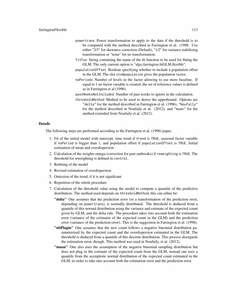
farringtonFlexible 113

powertrans Power transformation to apply to the data if the threshold is tobe computed with the method described in Farrington et al. (1996. Useeither "2/3" for skewness correction (Default), "1/2" for variance stabilizingtransformation or "none" for no transformation.

fitFun String containing the name of the fit function to be used for fitting theGLM. The only current option is "algo.farrington.fitGLM.flexible".

populationOffset Boolean specifying whether to include a population offsetin the GLM. The slot sts@population gives the population vector.

noPeriods Number of levels in the factor allowing to use more baseline. Ifequal to 1 no factor variable is created, the set of reference values is definedas in Farrington et al (1996).

pastWeeksNotIncluded Number of past weeks to ignore in the calculation.thresholdMethod Method to be used to derive the upperbound. Options are

"delta" for the method described in Farrington et al. (1996), "Noufaily"for the method described in Noufaily et al. (2012), and "muan" for themethod extended from Noufaily et al. (2012).

Details

The following steps are performed according to the Farrington et al. (1996) paper.

1. Fit of the initial model with intercept, time trend if trend is TRUE, seasonal factor variableif noPeriod is bigger than 1, and population offset if populationOffset is TRUE. Initialestimation of mean and overdispersion.

2. Calculation of the weights omega (correction for past outbreaks) if reweighting is TRUE. Thethreshold for reweighting is defined in control.

3. Refitting of the model

4. Revised estimation of overdispersion

5. Omission of the trend, if it is not significant

6. Repetition of the whole procedure

7. Calculation of the threshold value using the model to compute a quantile of the predictivedistribution. The method used depends on thresholdMethod, this can either be:

"delta" One assumes that the prediction error (or a transformation of the prediction error,depending on powertrans), is normally distributed. The threshold is deduced from aquantile of this normal distribution using the variance and estimate of the expected countgiven by GLM, and the delta rule. The procedure takes into account both the estimationerror (variance of the estimator of the expected count in the GLM) and the predictionerror (variance of the prediction error). This is the suggestion in Farrington et al. (1996).

"nbPlugin" One assumes that the new count follows a negative binomial distribution pa-rameterized by the expected count and the overdispersion estimated in the GLM. Thethreshold is deduced from a quantile of this discrete distribution. This process disregardsthe estimation error, though. This method was used in Noufaily, et al. (2012).

"muan" One also uses the assumption of the negative binomial sampling distribution butdoes not plug in the estimate of the expected count from the GLM, instead one uses aquantile from the asymptotic normal distribution of the expected count estimated in theGLM; in order to take into account both the estimation error and the prediction error.

114 farringtonFlexible

8. Computation of exceedance score

Warning: monthly data containing the last day of each month as date should be analysed withepochAsDate=FALSE in the sts object. Otherwise February makes it impossible to find some ref-erence time points.

Value

An object of class sts with the slots upperbound and alarm filled by appropriate output of thealgorithm. The slot control is the usual list but with more items all of length length(range):

trend is a vector of Booleans indicating whether a time trend was fitted for this time point.

trendVector is a vector giving the coefficient of the time trend in the GLM for this time point. Ifno trend was fitted it is equal to NA.

pvalue is a vector giving the probability of observing a value at least equal to the observation underthe null hypothesis .

expected is a vector giving the expectation of the predictive distribution for each timepoint. It isonly reported if the conditions for raising an alarm are met (enough cases).

mu0Vector is a vector giving what is inputed in the negative binomial distribution to get the upper-bound as a quantile (either a plug-in from the GLM or a quantile from the asymptotic normaldistribution of the estimator)

phiVector is a vector giving the overdispersion of the GLM at each timepoint.

Author(s)

M. Salmon, M. Höhle

References

Farrington, C.P., Andrews, N.J, Beale A.D. and Catchpole, M.A. (1996): A statistical algorithm forthe early detection of outbreaks of infectious disease. J. R. Statist. Soc. A, 159, 547-563.

Noufaily, A., Enki, D.G., Farrington, C.P., Garthwaite, P., Andrews, N.J., Charlett, A. (2012): Animproved algorithm for outbreak detection in multiple surveillance systems. Statistics in Medicine,32 (7), 1206-1222.


See Also

algo.farrington.fitGLM,algo.farrington.threshold

Examples

### DATA I/O ####Read Salmonella Agona datadata("salmonella.agona")



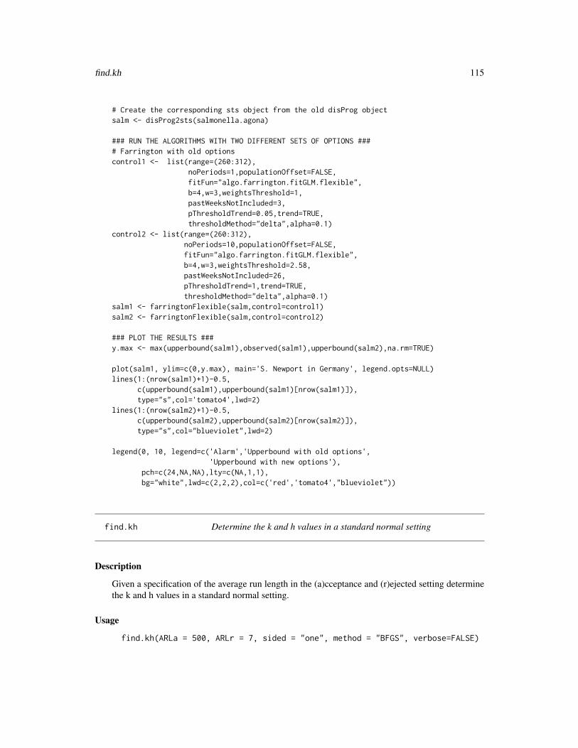
find.kh 115

# Create the corresponding sts object from the old disProg objectsalm <- disProg2sts(salmonella.agona)

### RUN THE ALGORITHMS WITH TWO DIFFERENT SETS OF OPTIONS #### Farrington with old optionscontrol1 <- list(range=(260:312),

noPeriods=1,populationOffset=FALSE,fitFun="algo.farrington.fitGLM.flexible",b=4,w=3,weightsThreshold=1,pastWeeksNotIncluded=3,pThresholdTrend=0.05,trend=TRUE,thresholdMethod="delta",alpha=0.1)

control2 <- list(range=(260:312),noPeriods=10,populationOffset=FALSE,fitFun="algo.farrington.fitGLM.flexible",b=4,w=3,weightsThreshold=2.58,pastWeeksNotIncluded=26,pThresholdTrend=1,trend=TRUE,thresholdMethod="delta",alpha=0.1)

salm1 <- farringtonFlexible(salm,control=control1)salm2 <- farringtonFlexible(salm,control=control2)

### PLOT THE RESULTS ###y.max <- max(upperbound(salm1),observed(salm1),upperbound(salm2),na.rm=TRUE)

plot(salm1, ylim=c(0,y.max), main='S. Newport in Germany', legend.opts=NULL)lines(1:(nrow(salm1)+1)-0.5,

c(upperbound(salm1),upperbound(salm1)[nrow(salm1)]),type="s",col='tomato4',lwd=2)

lines(1:(nrow(salm2)+1)-0.5,c(upperbound(salm2),upperbound(salm2)[nrow(salm2)]),type="s",col="blueviolet",lwd=2)

legend(0, 10, legend=c('Alarm','Upperbound with old options','Upperbound with new options'),

pch=c(24,NA,NA),lty=c(NA,1,1),bg="white",lwd=c(2,2,2),col=c('red','tomato4',"blueviolet"))

find.kh Determine the k and h values in a standard normal setting

Description

Given a specification of the average run length in the (a)cceptance and (r)ejected setting determinethe k and h values in a standard normal setting.

Usage

find.kh(ARLa = 500, ARLr = 7, sided = "one", method = "BFGS", verbose=FALSE)

116 findH

Arguments

ARLa average run length in acceptance setting, aka. in control state. Specifies thenumber of observations before false alarm.

ARLr average run length in rejection state, aka. out of control state. Specifies thenumber of observations before an increase is detected (i.e. detection delay)

sided one-sided cusum scheme

method Which method to use in the function optim. Standard choice is BFGS, but insome situation Nelder-Mead can be advantageous.

verbose gives extra information about the root finding process

Details

Functions from the spc package are used in a simple univariate root finding problem.

Value

Returns a list with reference value k and decision interval h.

Examples

if (requireNamespace("spc")) {find.kh(ARLa=500,ARLr=7,sided="one")find.kh(ARLa=500,ARLr=3,sided="one")

}

findH Find decision interval for given in-control ARL and reference value

Description

Function to find a decision interval h* for given reference value k and desired ARL γ so that theaverage run length for a Poisson or Binomial CUSUM with in-control parameter θ0, reference valuek and is approximately γ, i.e.

∣∣∣ARL(h∗)−γγ

∣∣∣ < ε, or larger, i.e. ARL(h∗) > γ.

Usage

findH(ARL0, theta0, s = 1, rel.tol = 0.03, roundK = TRUE,distr = c("poisson", "binomial"), digits = 1, FIR = FALSE, ...)

hValues(theta0, ARL0, rel.tol=0.02, s = 1, roundK = TRUE, digits = 1,distr = c("poisson", "binomial"), FIR = FALSE, ...)

findH 117

Arguments

ARL0 desired in-control ARL γ

theta0 in-control parameter θ0

s change to detect, see details


rel.tol relative tolerance, i.e. the search for h* is stopped if∣∣∣ARL(h∗)−γγ

∣∣∣ < rel.tol

digits the reference value k and the decision interval h are rounded to digits decimalplaces

roundK passed to findK

FIR if TRUE, the decision interval that leads to the desired ARL for a FIR CUSUMwith head start h2 is returned

... further arguments for the distribution function, i.e. number of trials n for bino-mial cdf

Details

The out-of-control parameter used to determine the reference value k is specified as:

θ1 = λ0 + s√λ0

for a Poisson variate X ∼ Po(λ)

θ1 =sπ0

1 + (s− 1)π0

for a Binomial variate X ∼ Bin(n, π)

Value

findH returns a vector and hValues returns a matrix with elements

theta0 in-control parameter

h decision interval

k reference value

ARL ARL for a CUSUM with parameters k and h

rel.tol corresponds to∣∣∣ARL(h)−γγ

∣∣∣

118 fluBYBW

findK Find Reference Value

Description

Calculates the reference value k for a Poisson or binomial CUSUM designed to detect a shift fromθ0 to θ1

Usage

findK(theta0, theta1, distr = c("poisson", "binomial"),roundK = FALSE, digits = 1, ...)

Arguments

theta0 in-control parameter

theta1 out-of-control parameter


digits the reference value k is rounded to digits decimal places

roundK For discrete data and rational reference value there is only a limited set of pos-sible values that the CUSUM can take (and therefore there is also only a limitedset of ARLs). If roundK=TRUE, integer multiples of 0.5 are avoided when round-ing the reference value k, i.e. the CUSUM can take more values.

... further arguments for the distribution function, i.e. number of trials n for thebinomial CDF.

Value

Returns reference value k.

fluBYBW Influenza in Southern Germany

Description

Weekly number of influenza A & B cases in the 140 districts of the two Southern German statesBavaria and Baden-Wuerttemberg, for the years 2001 to 2008. These surveillance data have beenanalyzed originally by Paul and Held (2011) and more recently by Meyer and Held (2014).

Usage

data(fluBYBW)

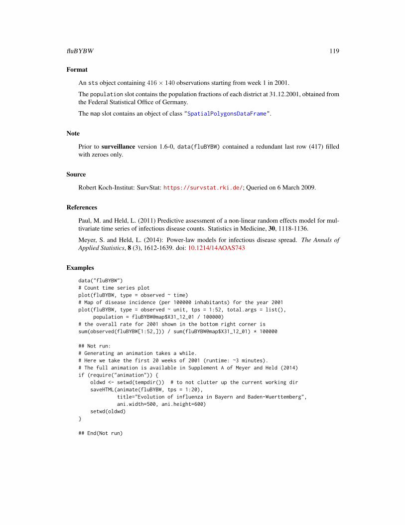
fluBYBW 119

Format

An sts object containing 416× 140 observations starting from week 1 in 2001.

The population slot contains the population fractions of each district at 31.12.2001, obtained fromthe Federal Statistical Office of Germany.

The map slot contains an object of class "SpatialPolygonsDataFrame".

Note

Prior to surveillance version 1.6-0, data(fluBYBW) contained a redundant last row (417) filledwith zeroes only.

Source

Robert Koch-Institut: SurvStat: https://survstat.rki.de/; Queried on 6 March 2009.

References

Paul, M. and Held, L. (2011) Predictive assessment of a non-linear random effects model for mul-tivariate time series of infectious disease counts. Statistics in Medicine, 30, 1118-1136.

Meyer, S. and Held, L. (2014): Power-law models for infectious disease spread. The Annals ofApplied Statistics, 8 (3), 1612-1639. doi: 10.1214/14AOAS743

Examples

data("fluBYBW")# Count time series plotplot(fluBYBW, type = observed ~ time)# Map of disease incidence (per 100000 inhabitants) for the year 2001plot(fluBYBW, type = observed ~ unit, tps = 1:52, total.args = list(),

population = fluBYBW@map$X31_12_01 / 100000)# the overall rate for 2001 shown in the bottom right corner issum(observed(fluBYBW[1:52,])) / sum(fluBYBW@map$X31_12_01) * 100000

## Not run:# Generating an animation takes a while.# Here we take the first 20 weeks of 2001 (runtime: ~3 minutes).# The full animation is available in Supplement A of Meyer and Held (2014)if (require("animation")) {

oldwd <- setwd(tempdir()) # to not clutter up the current working dirsaveHTML(animate(fluBYBW, tps = 1:20),

title="Evolution of influenza in Bayern and Baden-Wuerttemberg",ani.width=500, ani.height=600)

setwd(oldwd)}

## End(Not run)


http://doi.org/10.1214/14-AOAS743

120 glm_epidataCS

formatPval Pretty p-Value Formatting

Description

Just YAPF – yet another p-value formatter...

It is a wrapper around format.pval, such that by default eps = 1e-4, scientific = FALSE,digits = if (p<10*eps) 1 else 2, and nsmall = 2.

Usage

formatPval(pv, eps = 1e-4, scientific = FALSE, ...)

Arguments

pv a numeric vector (of p-values).

eps a numerical tolerance, see format.pval.

scientific see format.

... further arguments passed to format.pval (but digits and nsmall are hard-coded internally).

Value

The character vector of formatted p-values.

Examples

formatPval(c(0.9, 0.13567, 0.0432, 0.000546, 1e-8))

glm_epidataCS Fit an Endemic-Only twinstim as a Poisson-glm

Description

An endemic-only twinstim is equivalent to a Poisson regression model for the aggregated numberof events, Y[t][s],k, by time-space-type cell. The rate of the corresponding Poisson distribution ise[t][s] ·λ([t], [s], k), where e[t][s] = |[t]||[s]| is a multiplicative offset. Thus, the glm function can beused to fit an endemic-only twinstim. However, wrapping in glm is usually slower.

Usage

glm_epidataCS(formula, data, ...)

glm_epidataCS 121

Arguments

formula an endemic model formula without response, comprising variables of data$stgridand possibly the variable type for a type-specific model.

data an object of class "epidataCS".

... arguments passed to glm. Note that family and offset are fixed internally.

Value

a glm

Author(s)

Sebastian Meyer

Examples

data("imdepi", "imdepifit")

## Fit an endemic-only twinstim() and an equivalent model wrapped in glm()fit_twinstim <- update(imdepifit, epidemic = ~0, siaf = NULL, subset = NULL,

optim.args=list(control=list(trace=0)), verbose=FALSE)fit_glm <- glm_epidataCS(formula(fit_twinstim)$endemic, data = imdepi)

## Compare the coefficientscbind(twinstim = coef(fit_twinstim), glm = coef(fit_glm))

### also compare to an equivalent endemic-only hhh4() fit

## first need to aggregate imdepi into an "sts" objectload(system.file("shapes", "districtsD.RData", package="surveillance"))imdsts <- epidataCS2sts(imdepi, freq = 12, start = c(2002, 1),

neighbourhood = NULL, tiles = districtsD,popcol.stgrid = "popdensity")

## determine the correct offset to get an equivalent modeloffset <- 2 * rep(with(subset(imdepi$stgrid, !duplicated(BLOCK)),

stop - start), ncol(imdsts)) *sum(districtsD$POPULATION) * population(imdsts)

## fit the model using hhh4()fit_hhh4 <- hhh4(imdsts, control = list(

end = list(f = addSeason2formula(~I(start/365-3.5), period=365, timevar="start"),offset = offset

), family = "Poisson", subset = 1:nrow(imdsts),data = list(start=with(subset(imdepi$stgrid, !duplicated(BLOCK)), start))))

summary(fit_hhh4)stopifnot(all.equal(coef(fit_hhh4), coef(fit_glm), check.attributes=FALSE))

122 ha

ha Hepatitis A in Berlin

Description

Number of Hepatitis A cases among adult male (age>18) in Berlin 2001-2006. An increase is seenduring 2006

Usage

data("ha")data("ha.sts")

Format

ha is a disProg object containing 290 × 12 observations starting from week 1 in 2001 to week 30in 2006. ha.sts is generated from ha by the converter function disProg2sts using a shape file ofBerlin (see Examples).

Source

Robert Koch-Institut: SurvStat: https://survstat.rki.de/; Queried on 25 August 2006.

Robert Koch Institut, Epidemiologisches Bulletin 33/2006, p.290.

Examples

## deprecated "disProg" objectdata("ha")haplot(aggregate(ha))

## new-style "sts" objectdata("ha.sts")ha.stsplot(ha.sts, type = observed ~ unit, labels = TRUE)

## conversion of the old "disProg" object 'ha' to the new S4 class "sts"## Not run:shpfile <- system.file("shapes/berlin.shp", package="surveillance")ha.sts <- disProg2sts(ha, map = maptools::readShapePoly(shpfile,IDvar="SNAME"))## in data("ha.sts"), German umlauts in 'ha.sts@map@data$BEZIRK'## have been replaced for compatibility

## End(Not run)


hagelloch 123

hagelloch 1861 Measles Epidemic in the City of Hagelloch, Germany

Description

Data on the 188 cases in the measles outbreak among children in the German city of Hagelloch(near Tübingen) 1861. The data were originally collected by Dr. Albert Pfeilsticker (1863) andaugmented and re-analysed by Dr. Heike Oesterle (1992).

Usage

data("hagelloch")

Format

Loading data("hagelloch") gives two objects: hagelloch and hagelloch.df. The former is an"epidata" object for use with twinSIR containing the entire SIR event history of the outbreak inthe population of 188 children. The latter is the original data.frame of 188 rows with individualinformation for each infected child.

The covariate information in hagelloch.df is as follows:

PN: patient number

NAME: patient name (as a factor)

FN: family index

HN: house number

AGE: age in years

SEX: gender of the individual (factor: male, female)

PRO: Date of prodromes

ERU: Date of rash

CL: class (factor: preschool, 1st class, 2nd class)

DEAD: Date of death (with missings)

IFTO: number of patient who is the putative source of infection (0 = unknown)

SI: serial interval = number of days between dates of prodromes of infection source and infectedperson

C: complications (factor: no complications, bronchopneumonia, severe bronchitis, lobar pneumo-nia, pseudocroup, cerebral edema)

PR: duration of prodromes in days

CA: number of cases in family

NI: number of initial cases

GE: generation number of the case

TD: day of max. fever (days after rush)

124 hagelloch

TM: max. fever (degree Celsius)

x.loc: x coordinate of house (in meters). Scaling in metres is obtained by multiplying the originalcoordinates by 2.5 (see details in Neal and Roberts (2004))

y.loc: y coordinate of house (in meters). See also the above description of x.loc.

tPRO: Time of prodromes (first symptoms) in days after the start of the epidemic (30 Oct 1861).

tERU: Time upon which the rash first appears.

tDEAD: Time of death, if available.

tR: Time at which the infectious period of the individual is assumed to end. This unknown time iscalculated as

tRi = min tDEADi, tERUi + d0,

where – as in Section 3.1 of Neal and Roberts (2004) – we use d0 = 3.

tI: Time at which the individual is assumed to become infectious. Actually this time is unknown,but we use

tIi = tPROi − d1,

where d1 = 1 as in Neal and Roberts (2004).

The time variables describe the transitions of the individual in an Susceptible-Infectious-Recovered(SIR) model. Note that in order to avoid ties in the event times resulting from daily interval cen-soring, the times have been jittered uniformly within the respective day. The time point 0.5 wouldcorrespond to noon of 30 Oct 1861.

The hagelloch "epidata" object only retains some of the above covariates to save space. Apartfrom the usual "epidata" event columns, hagelloch contains a number of extra variables repre-senting distance- and covariate-based weights for the force of infection. These have been computedby specifying f and w arguments in as.epidata at conversion (see the Examples below):

household: the number of currently infectious children in the same household (including the childitself if it is currently infectious), corresponding to function(u) u == 0 in f.

nothousehold: the number of currently infectious children outside the household, correspondingto function(u) u > 0 in f.

c1, c2: the number of children infectious during the respective time block and being members ofclass 1 and 2, respectively; but the value is 0 if the individual of the row is not herself a memberof the respective class. See the Examples below for the corresponding function definitions inw.

Source

Thanks to Peter J. Neal, University of Manchester, for providing us with these data, which he againbecame from Niels Becker, Australian National University. To cite the data, the main references arePfeilsticker (1863) and Oesterle (1992).

References

Pfeilsticker, A. (1863). Beiträge zur Pathologie der Masern mit besonderer Berücksichtigung derstatistischen Verhältnisse, M.D. Thesis, Eberhard-Karls-Universität Tübingen. Available as http://www.archive.org/details/beitrgezurpatho00pfeigoog.

http://www.archive.org/details/beitrgezurpatho00pfeigoog

http://www.archive.org/details/beitrgezurpatho00pfeigoog

hagelloch 125

Oesterle, H. (1992). Statistische Reanalyse einer Masernepidemie 1861 in Hagelloch, M.D. Thesis,Eberhard-Karls-Universitäat Tübingen.

Neal, P. J. and Roberts, G. O (2004). Statistical inference and model selection for the 1861 Hagel-loch measles epidemic, Biostatistics 5(2):249-261

See Also

twinSIR, epidata

Examples

data("hagelloch")

head(hagelloch.df) # original data documented in Oesterle (1992)head(as.data.frame(hagelloch)) # derived "epidata" object

### How the "epidata" 'hagelloch' was created from 'hagelloch.df'

stopifnot(all.equal(hagelloch,as.epidata(hagelloch.df, t0 = 0, tI.col = "tI", tR.col = "tR",id.col = "PN", coords.cols = c("x.loc", "y.loc"),f = list(

household = function(u) u == 0,nothousehold = function(u) u > 0

),w = list(

c1 = function (CL.i, CL.j) CL.i == "1st class" & CL.j == CL.i,c2 = function (CL.i, CL.j) CL.i == "2nd class" & CL.j == CL.i

),keep.cols = c("SEX", "AGE", "CL"))

))

### Basic plots produced from hagelloch.df

# Show case locations as in Neal & Roberts (different scaling) using# the data.frame (promoted to a SpatialPointsDataFrame)coordinates(hagelloch.df) <- c("x.loc","y.loc")plot(hagelloch.df, xlab="x [m]", ylab="x [m]", pch=15, axes=TRUE,

cex=sqrt(multiplicity(hagelloch.df)))

# Epicurvehist(as.numeric(hagelloch.df$tI), xlab="Time (days)", ylab="Cases", main="")

### SIR model information for population & individuals

(s <- summary(hagelloch))plot(s, col=c("green","red","darkgray"))stateplot(s, id=c("187"))

126 hcl.colors

## Not run:# Show a dynamic illustration of the spread of the infectionanimate(hagelloch,time.spacing=0.1,legend.opts=list(x="topleft"),sleep=1/100)

## End(Not run)

hcl.colors HCL-based Heat Colors from the colorspace Package

Description

If package colorspace is available, its heat_hcl function is used to generate a color palette. Other-wise, the function simply calls heat.colors (or grey.colors if use.color=FALSE).

Usage

hcl.colors(ncolors = 100, use.color = TRUE)

Arguments

ncolors the number of colors (>= 1) to be in the palette.

use.color logical. Should the palette use colors? Otherwise grey levels are returned.

Value

A character vector of ncolors colors.

See Also

heat_hcl in package colorspace, or heat.colors in the base package grDevices.

Examples

barplot(rep(1,10), col = hcl.colors(10), axes = FALSE)

hepatitisA 127

hepatitisA Hepatitis A in Germany

Description

Weekly number of reported hepatitis A infections in Germany 2001-2004.

Usage

data(hepatitisA)

Format

A disProg object containing 208×1 observations starting from week 1 in 2001 to week 52 in 2004.

Source

Robert Koch-Institut: SurvStat: https://survstat.rki.de/; Queried on 11-01-2005.

Examples

data(hepatitisA)plot(hepatitisA)

hhh4 Fitting HHH Models with Random Effects and Neighbourhood Struc-ture

Description

Fits an autoregressive Poisson or negative binomial model to a univariate or multivariate time seriesof counts. The characteristic feature of hhh4 models is the additive decomposition of the conditionalmean into epidemic and endemic components (Held et al, 2005). Log-linear predictors of covariatesand random intercepts are allowed in all components; see the Details below. A general introductionto the hhh4 modelling approach and its implementation is given in the vignette("hhh4"). Meyeret al (2017, Section 5, available as vignette("hhh4_spacetime")) describe hhh4 models for arealtime series of infectious disease counts.

Usage

hhh4(stsObj,control = list(

ar = list(f = ~ -1, offset = 1, lag = 1),ne = list(f = ~ -1, offset = 1, lag = 1,

weights = neighbourhood(stsObj) == 1,scale = NULL, normalize = FALSE),


128 hhh4

end = list(f = ~ 1, offset = 1),family = c("Poisson", "NegBin1", "NegBinM"),subset = 2:nrow(stsObj),optimizer = list(stop = list(tol=1e-5, niter=100),

regression = list(method="nlminb"),variance = list(method="nlminb")),

verbose = FALSE,start = list(fixed=NULL, random=NULL, sd.corr=NULL),data = list(t = stsObj@epoch - min(stsObj@epoch)),keep.terms = FALSE

),check.analyticals = FALSE)

Arguments

stsObj object of class "sts" containing the (multivariate) count data time series.

control a list containing the model specification and control arguments:

ar Model for the autoregressive component given as list with the followingcomponents:f = ~ -1 a formula specifying log(λit)

offset = 1 optional multiplicative offset, either 1 or a matrix of the samedimension as observed(stsObj)

lag = 1 a positive integer meaning autoregression on yi,t−lagne Model for the neighbour-driven component given as list with the following

components:f = ~ -1 a formula specifying log(φit)

offset = 1 optional multiplicative offset, either 1 or a matrix of the samedimension as observed(stsObj)

lag = 1 a non-negative integer meaning dependency on yj,t−lagweights = neighbourhood(stsObj) == 1 neighbourhood weightswji. The

default corresponds to the original formulation by Held et al (2005),i.e., the spatio-temporal component incorporates an unweighted sumover the lagged cases of the first-order neighbours. See Paul et al(2008) and Meyer and Held (2014) for alternative specifications, e.g.,W_powerlaw. Time-varying weights are possible by specifying an arrayof dim() c(nUnits, nUnits, nTime), where nUnits=ncol(stsObj)and nTime=nrow(stsObj).

scale = NULL optional matrix of the same dimensions as weights (or avector of length ncol(stsObj)) to scale the weights to scale * weights.

normalize = FALSE logical indicating if the (scaled) weights should benormalized such that each row sums to 1.

end Model for the endemic component given as list with the following compo-nentsf = ~ 1 a formula specifying log(νit)

offset = 1 optional multiplicative offset eit, either 1 or a matrix of the samedimension as observed(stsObj)

hhh4 129

family Distributional family – either "Poisson", or the Negative Binomial dis-tribution. For the latter, the overdispersion parameter can be assumed to bethe same for all units ("NegBin1"), to vary freely over all units ("NegBinM"),or to be shared by some units (specified by a factor of length ncol(stsObj)such that its number of levels determines the number of overdispersion pa-rameters). Note that "NegBinM" is equivalent to factor(colnames(stsObj), levels = colnames(stsObj)).

subset Typically 2:nrow(obs) if model contains autoregressionoptimizer a list of three lists of control arguments.

The "stop" list specifies two criteria for the outer optimization of regres-sion and variance parameters: the relative tolerance for parameter changeusing the criterion max(abs(x[i+1]-x[i])) / max(abs(x[i])), and themaximum number niter of outer iterations.Control arguments for the single optimizers are specified in the lists named"regression" and "variance". method="nlminb" is the default opti-mizer for both (taking advantage of the analytical Fisher information ma-trices), however, the methods from optim may also be specified (as well as"nlm" but that one is not recommended here). Especially for the varianceupdates, Nelder-Mead optimization (method="Nelder-Mead") is an attrac-tive alternative. All other elements of these two lists are passed as controlarguments to the chosen method, e.g., if method="nlminb" adding iter.max=50increases the maximum number of inner iterations from 20 (default) to 50.

verbose non-negative integer (usually in the range 0:3) specifying the amountof tracing information to be output during optimization.

start a list of initial parameter values replacing initial values set via fe and ri.Since surveillance 1.8-2, named vectors are matched against the coefficientnames in the model (where unmatched start values are silently ignored), andneed not be complete, e.g., start = list(fixed = c("-log(overdisp)" = 0.5))(default: 2) for a family = "NegBin1" model. In contrast, an unnamedstart vector must specify the full set of parameters as used by the model.

data a named list of covariates that are to be included as fixed effects (see fe)in any of the 3 component formulae. By default, the time variable t isavailable and used for seasonal effects created by addSeason2formula. Ingeneral, covariates in this list can be either vectors of length nrow(stsObj)interpreted as time-varying but common across all units, or matrices of thesame dimension as the disease counts observed(stsObj).

keep.terms logical indicating if the terms object used in the fit is to be kept aspart of the returned object. This is usually not necessary, since the termsobject is reconstructed by the terms-method for class "hhh4" if necessary(based on stsObj and control, which are both part of the returned "hhh4"object).

The auxiliary function makeControl might be useful to create such a list ofcontrol parameters.

check.analyticals

logical (or a subset of c("numDeriv", "maxLik")), indicating if (how) theimplemented analytical score vector and Fisher information matrix should bechecked against numerical derivatives at the parameter starting values, using thepackages numDeriv and/or maxLik. If activated, hhh4 will return a list contain-ing the analytical and numerical derivatives for comparison (no ML estimation

130 hhh4

will be performed). This is mainly intended for internal use by the packagedevelopers.

Details

An endemic-epidemic multivariate time-series model for infectious disease counts Yit from unitsi = 1, . . . , I during periods t = 1, . . . , T was proposed by Held et al (2005) and was later extendedin a series of papers (Paul et al, 2008; Paul and Held, 2011; Held and Paul, 2012; Meyer and Held,2014). In its most general formulation, this so-called hhh4 (or HHH or H3 or triple-H) modelassumes that, conditional on past observations, Yit has a Poisson or negative binomial distributionwith mean

µit = λityi,t−1 + φit∑j 6=i

wjiyj,t−1 + eitνit

In the case of a negative binomial model, the conditional variance is µit(1+ψiµit) with overdisper-sion parameters ψi > 0 (possibly shared across different units, e.g., ψi ≡ ψ). Univariate time seriesof counts Yt are supported as well, in which case hhh4 can be regarded as an extension of glm.nbto account for autoregression. See the Examples below for a comparison of an endemic-only hhh4model with a corresponding glm.nb.

The three unknown quantities of the mean µit,

• λit in the autoregressive (ar) component,

• φit in the neighbour-driven (ne) component, and

• νit in the endemic (end) component,

are log-linear predictors incorporating time-/unit-specific covariates. They may also contain unit-specific random intercepts as proposed by Paul and Held (2011). The endemic mean is usuallymodelled proportional to a unit-specific offset eit (e.g., population numbers or fractions); it is pos-sible to include such multiplicative offsets in the epidemic components as well. The wji are trans-mission weights reflecting the flow of infections from unit j to unit i. In spatial hhh4 applications,the “units” refer to geographical regions and the weights could be derived from movement networkdata. Alternatively, the weights can be estimated parametrically as a function of adjacency order(Meyer and Held, 2014).

(Penalized) Likelihood inference for such hhh4 models has been established by Paul and Held(2011) with extensions for parametric neighbourhood weights by Meyer and Held (2014). Suppliedwith the analytical score function and Fisher information, the function hhh4 by default uses thequasi-Newton algorithm available through nlminb to maximize the log-likelihood. Convergenceis usually fast even for a large number of parameters. If the model contains random effects, thepenalized and marginal log-likelihoods are maximized alternately until convergence.

Value

hhh4 returns an object of class "hhh4", which is a list containing the following components:

coefficients named vector with estimated (regression) parameters of the model

se estimated standard errors (for regression parameters)

cov covariance matrix (for regression parameters)

Sigma estimated variance-covariance matrix of random effects

hhh4 131

Sigma.orig estimated variance parameters on internal scale used for optimization

Sigma.cov inverse of marginal Fisher information (on internal scale), i.e., the asymptoticcovariance matrix of Sigma.orig

call the matched call

dim vector with number of fixed and random effects in the model

loglikelihood (penalized) loglikelihood evaluated at the MLE

margll (approximate) log marginal likelihood should the model contain random effects

convergence logical. Did optimizer converge?

fitted.values fitted mean values µi,tcontrol control object of the fit

terms the terms object used in the fit if keep.terms = TRUE and NULL otherwise

stsObj the supplied stsObj

lags named integer vector of length two containing the lags used for the epidemiccomponents "ar" and "ne", respectively. The corresponding lag is NA if thecomponent was not included in the model.

nObs number of observations used for fitting the model

nTime number of time points used for fitting the model

nUnit number of units (e.g. areas) used for fitting the model

runtime the proc.time-queried time taken to fit the model, i.e., a named numeric vectorof length 5 of class "proc_time"

Author(s)

Michaela Paul, Sebastian Meyer, Leonhard Held

References

Held, L., Höhle, M. and Hofmann, M. (2005): A statistical framework for the analysis of multi-variate infectious disease surveillance counts. Statistical Modelling, 5 (3), 187-199. doi: 10.1191/1471082X05st098oa

Paul, M., Held, L. and Toschke, A. M. (2008): Multivariate modelling of infectious disease surveil-lance data. Statistics in Medicine, 27 (29), 6250-6267. doi: 10.1002/sim.4177

Paul, M. and Held, L. (2011): Predictive assessment of a non-linear random effects model formultivariate time series of infectious disease counts. Statistics in Medicine, 30 (10), 1118-1136.doi: 10.1002/sim.4177

Held, L. and Paul, M. (2012): Modeling seasonality in space-time infectious disease surveillancedata. Biometrical Journal, 54 (6), 824-843. doi: 10.1002/bimj.201200037



http://doi.org/10.1191/1471082X05st098oa

http://doi.org/10.1191/1471082X05st098oa

http://doi.org/10.1002/sim.4177


http://doi.org/10.1002/bimj.201200037




132 hhh4

See Also

See the special functions fe, ri and the examples below for how to specify unit-specific effects.

Further details on the modelling approach and illustrations of its implementation can be found invignette("hhh4") and vignette("hhh4_spacetime").

Examples

######################## Univariate examples######################

### weekly counts of salmonella agona cases, UK, 1990-1995

data("salmonella.agona")## convert old "disProg" to new "sts" data classsalmonella <- disProg2sts(salmonella.agona)salmonellaplot(salmonella)

## generate formula for an (endemic) time trend and seasonalityf.end <- addSeason2formula(f = ~1 + t, S = 1, period = 52)f.end## specify a simple autoregressive negative binomial modelmodel1 <- list(ar = list(f = ~1), end = list(f = f.end), family = "NegBin1")## fit this model to the datares <- hhh4(salmonella, model1)## summarize the model fitsummary(res, idx2Exp=1, amplitudeShift=TRUE, maxEV=TRUE)plot(res)plot(res, type = "season", components = "end")

### weekly counts of meningococcal infections, Germany, 2001-2006

data("influMen")fluMen <- disProg2sts(influMen)meningo <- fluMen[, "meningococcus"]meningoplot(meningo)

## again a simple autoregressive NegBin model with endemic seasonalitymeningoFit <- hhh4(stsObj = meningo, control = list(

ar = list(f = ~1),end = list(f = addSeason2formula(f = ~1, S = 1, period = 52)),family = "NegBin1"

))

summary(meningoFit, idx2Exp=TRUE, amplitudeShift=TRUE, maxEV=TRUE)plot(meningoFit)plot(meningoFit, type = "season", components = "end")

hhh4 133

########################## Multivariate examples########################

### bivariate analysis of influenza and meningococcal infections### (see Paul et al, 2008)

plot(fluMen, same.scale = FALSE)

## Fit a negative binomial model with## - autoregressive component: disease-specific intercepts## - neighbour-driven component: only transmission from flu to men## - endemic component: S=3 and S=1 sine/cosine pairs for flu and men, respectively## - disease-specific overdispersion

WfluMen <- neighbourhood(fluMen)WfluMen["meningococcus","influenza"] <- 0WfluMenf.end_fluMen <- addSeason2formula(f = ~ -1 + fe(1, which = c(TRUE, TRUE)),

S = c(3, 1), period = 52)f.end_fluMenfluMenFit <- hhh4(fluMen, control = list(

ar = list(f = ~ -1 + fe(1, unitSpecific = TRUE)),ne = list(f = ~ 1, weights = WfluMen),end = list(f = f.end_fluMen),family = "NegBinM"))

summary(fluMenFit, idx2Exp=1:3)plot(fluMenFit, type = "season", components = "end", unit = 1)plot(fluMenFit, type = "season", components = "end", unit = 2)

### weekly counts of measles, Weser-Ems region of Lower Saxony, Germany

data("measlesWeserEms")measlesWeserEmsplot(measlesWeserEms) # note the two districts with zero cases

## we could fit the same simple model as for the salmonella cases abovemodel1 <- list(

ar = list(f = ~1),end = list(f = addSeason2formula(~1 + t, period = 52)),family = "NegBin1"

)measlesFit <- hhh4(measlesWeserEms, model1)summary(measlesFit, idx2Exp=TRUE, amplitudeShift=TRUE, maxEV=TRUE)

## but we should probably at least use a population offset in the endemic## component to reflect heterogeneous incidence levels of the districts,## and account for spatial dependence (here just using first-order adjacency)measlesFit2 <- update(measlesFit,

end = list(offset = population(measlesWeserEms)),ne = list(f = ~1, weights = neighbourhood(measlesWeserEms) == 1))

summary(measlesFit2, idx2Exp=TRUE, amplitudeShift=TRUE, maxEV=TRUE)

134 hhh4

plot(measlesFit2, units = NULL, hide0s = TRUE)

## 'measlesFit2' corresponds to the 'measlesFit_basic' model in## vignette("hhh4_spacetime"). See there for further analyses,## including vaccination coverage as a covariate,## spatial power-law weights, and random intercepts.

## Not run:### last but not least, a more sophisticated (and time-consuming)### analysis of weekly counts of influenza from 140 districts in### Southern Germany (originally analysed by Paul and Held, 2011,### and revisited by Held and Paul, 2012, and Meyer and Held, 2014)

data("fluBYBW")plot(fluBYBW, type = observed ~ time)plot(fluBYBW, type = observed ~ unit,

## mean yearly incidence per 100.000 inhabitants (8 years)population = fluBYBW@map$X31_12_01 / 100000 * 8)

## For the full set of models for data("fluBYBW") as analysed by## Paul and Held (2011), including predictive model assessement## using proper scoring rules, see the (computer-intensive)## demo("fluBYBW") script:demoscript <- system.file(file.path("demo", "fluBYBW.R"),

package = "surveillance")demoscript#file.show(demoscript)

## Here we fit the improved power-law model of Meyer and Held (2014)## - autoregressive component: random intercepts + S = 1 sine/cosine pair## - neighbour-driven component: random intercepts + S = 1 sine/cosine pair## + population gravity with normalized power-law weights## - endemic component: random intercepts + trend + S = 3 sine/cosine pairs## - random intercepts are iid but correlated between componentsf.S1 <- addSeason2formula(

~-1 + ri(type="iid", corr="all"),S = 1, period = 52)

f.end.S3 <- addSeason2formula(~-1 + ri(type="iid", corr="all") + I((t-208)/100),S = 3, period = 52)

## for power-law weights, we need adjaceny orders, which can be## computed from the binary adjacency indicator matrixnbOrder1 <- neighbourhood(fluBYBW)neighbourhood(fluBYBW) <- nbOrder(nbOrder1, 15)

## full model specificationfluModel <- list(

ar = list(f = f.S1),ne = list(f = update.formula(f.S1, ~ . + log(pop)),

weights = W_powerlaw(maxlag=max(neighbourhood(fluBYBW)),normalize = TRUE, log = TRUE)),

hhh4 135

end = list(f = f.end.S3, offset = population(fluBYBW)),family = "NegBin1", data = list(pop = population(fluBYBW)),optimizer = list(variance = list(method = "Nelder-Mead")),verbose = TRUE)

## CAVE: random effects considerably increase the runtime of model estimation## (It is usually advantageous to first fit a model with simple intercepts## to obtain reasonable start values for the other parameters.)set.seed(1) # because random intercepts are initialized randomlyfluFit <- hhh4(fluBYBW, fluModel)

summary(fluFit, idx2Exp=TRUE, amplitudeShift=TRUE)

plot(fluFit, type = "season")

plot(fluFit, type = "neweights", xlab = "adjacency order")

gridExtra::grid.arrange(grobs = lapply(c("ar", "ne", "end"), function (comp)

plot(fluFit, type = "ri", component = comp, main = comp,at = seq(-2.6, 2.6, length.out = 15),col.regions = cm.colors(14))),

nrow = 1, ncol = 3)

range(plot(fluFit, type = "maxEV"))

## End(Not run)

########################################################################## An endemic-only "hhh4" model can also be estimated using MASS::glm.nb########################################################################

## weekly counts of measles, Weser-Ems region of Lower Saxony, Germanydata("measlesWeserEms")

## fit an endemic-only "hhh4" model## with time covariates and a district-specific offsethhh4fit <- hhh4(measlesWeserEms, control = list(

end = list(f = addSeason2formula(~1 + t, period = measlesWeserEms@freq),offset = population(measlesWeserEms)),

ar = list(f = ~-1), ne = list(f = ~-1), family = "NegBin1",subset = 1:nrow(measlesWeserEms)

))summary(hhh4fit)

## fit the same model using MASS::glm.nbmeaslesWeserEmsData <- as.data.frame(measlesWeserEms, tidy = TRUE)measlesWeserEmsData$t <- c(hhh4fit$control$data$t)glmnbfit <- MASS::glm.nb(

update(formula(hhh4fit)$end, observed ~ . + offset(log(population))),data = measlesWeserEmsData

)

136 hhh4_formula

summary(glmnbfit)

## Note that the overdispersion parameter is parametrized inversely.## The likelihood and point estimates are all the same.## However, the variance estimates are different: in glm.nb, the parameters## are estimated conditional on the overdispersion theta.

hhh4_formula Specify Formulae in a Random Effects HHH Model

Description

The special functions fe and ri are used to specify unit-specific effects of covariates and randomintercept terms, respectively, in the component formulae of hhh4.

Usage

fe(x, unitSpecific = FALSE, which = NULL, initial = NULL)

ri(type = c("iid","car"), corr = c("none", "all"),initial.fe = 0, initial.var = -.5, initial.re = NULL)

Arguments

x an expression like sin(2*pi*t/52) involving the time variable t, or just 1 for anintercept. In general this covariate expression might use any variables containedin the control$data argument of the parent hhh4 call.

unitSpecific logical indicating if the effect of x should be unit-specific. This is a convenientshortcut for which = rep(TRUE, nUnits), where nUnits is the number ofunits (i.e., columns of the "sts" object).

which vector of logicals indicating which unit(s) should get an unit-specific parameter.For units with a FALSE value, the effect term for x will be zero in the log-linearpredictor. Note especially that setting a FALSE value for the intercept term ofa unit, e.g., ar = list(f = ~-1 + fe(1, which=c(TRUE, FALSE))) in abivariate hhh4 model, does not mean that the (autoregressive) model componentis omitted for this unit, but that log(λ1) = α1 and log(λ2) = 0, which is usuallynot of interest. ATM, omitting an autoregressive effect for a specific unit is notpossible.If which=NULL, the parameter is assumed to be the same for all units.

initial initial values (on internal scale!) for the fixed effects used for optimization. Thedefault (NULL) means to use zeroes.

type random intercepts either follow an IID or a CAR model.

corr whether random effects in different components (such as ar and end) should becorrelated or not.

hhh4_methods 137

initial.fe initial value for the random intercept mean.

initial.var initial values (on internal scale!) for the variance components used for optimiza-tion.

initial.re initial values (on internal scale!) for the random effects used for optimization.The default NULL are random numbers from a normal distribution with zeromean and variance 0.001.

Note

These special functions are intended for use in component formulae of hhh4 models and are notexported from the package namespace.

If unit-specific fixed or random intercepts are specified, an overall intercept must be excluded (by-1) in the component formula.

See Also

addSeason2formula

hhh4 model specifications in vignette("hhh4"), vignette("hhh4_spacetime") or on the helppage of hhh4.

hhh4_methods Print, Summary and other Standard Methods for "hhh4" Objects

Description

Besides print and summary methods there are also some standard extraction methods defined forobjects of class "hhh4" resulting from a call to hhh4. The implementation is illustrated in Meyer etal. (2017, Section 5), see vignette("hhh4_spacetime").

Usage

## S3 method for class 'hhh4'print(x, digits = max(3, getOption("digits") - 3), ...)## S3 method for class 'hhh4'summary(object, maxEV = FALSE, ...)

## S3 method for class 'hhh4'coef(object, se = FALSE, reparamPsi = TRUE,

idx2Exp = NULL, amplitudeShift = FALSE, ...)## S3 method for class 'hhh4'fixef(object, ...)## S3 method for class 'hhh4'ranef(object, tomatrix = FALSE, ...)## S3 method for class 'hhh4'coeflist(x, ...)

138 hhh4_methods

## S3 method for class 'hhh4'formula(x, ...)## S3 method for class 'hhh4'nobs(object, ...)## S3 method for class 'hhh4'logLik(object, ...)

## S3 method for class 'hhh4'vcov(object, reparamPsi = TRUE,

idx2Exp = NULL, amplitudeShift = FALSE, ...)## S3 method for class 'hhh4'confint(object, parm, level = 0.95,

reparamPsi = TRUE, idx2Exp = NULL, amplitudeShift = FALSE, ...)

Arguments

x, object an object of class "hhh4".

digits the number of significant digits to use when printing

maxEV logical indicating if the summary should contain the (range of the) dominanteigenvalue as a measure of the importance of the epidemic components. Bydefault, the value is not calculated as this may take some seconds depending onthe number of time points and units in object$stsObj.

... For the print, summary, fixef, ranef, and coeflist methods: argumentspassed to coef.For the remaining methods: unused (argument of the generic).

reparamPsi logical. If TRUE (default), the overdispersion parameter from the negative bi-nomial distribution is transformed from internal scale (-log) to standard scale,where zero corresponds to a Poisson distribution.

se logical switch indicating if standard errors are required

idx2Exp integer vector selecting the parameters which should be returned on exp-scale.Alternatively, idx2Exp = TRUE will exp-transform all parameters except forthose associated with log() covariates or already affected by reparamPsi oramplitudeShift.

amplitudeShift logical switch indicating whether the parameters for sine/cosine terms modellingseasonal patterns (see addSeason2formula) should be transformed to an ampli-tude/shift formulation.

tomatrix logical. If FALSE (default), the vector of all random effects is returned (as usedinternally). However, for random intercepts of type="car", the number of pa-rameters is one less than the number of regions and the individual parametersare not obviously linked to specific regions. Setting tomatrix to TRUE returns amore useful representation of random effects in a matrix with as many rows asthere are regions and as many columns as there are random effects. Here, anyCAR-effects are transformed to region-specific effects.

parm a vector of numbers or names, specifying which parameters are to be givenconfidence intervals. If missing, all parameters are considered.

level the confidence level required.

hhh4_predict 139

Value

The coef-method returns all estimated (regression) parameters from a hhh4 model. If the modelincludes random effects, those can be extracted with ranef, whereas fixef returns the fixed pa-rameters. The coeflist-method extracts the model coefficients in a list (by parameter group).

The formula-method returns the formulae used for the three log-linear predictors in a list withelements "ar", "ne", and "end". The nobs-method returns the number of observations used formodel fitting. The logLik-method returns an object of class "logLik" with "df" and "nobs"attributes. For a random effects model, the value of the penalized log-likelihood at the MLE isreturned, but degrees of freedom are not available (NA_real_). As a consequence, AIC and BIC areonly well defined for models without random effects; otherwise these functions return NA_real_.

The vcov-method returns the estimated variance-covariance matrix of the regression parameters.The estimated variance-covariance matrix of random effects is available as object$Sigma. Theconfint-method returns Wald-type confidence intervals (assuming asymptotic normality).

Author(s)

Michaela Paul and Sebastian Meyer

References


See Also

the plot and update methods for fitted "hhh4" models.

hhh4_predict Predictions from a hhh4 Model

Description

Get fitted (component) means from a hhh4 model.

Usage

## S3 method for class 'hhh4'predict(object, newSubset=object$control$subset,

type="response", ...)



140 hhh4_simulate

Arguments

object fitted hhh4 model (class "hhh4").

newSubset subset of time points for which to return the predictions. Defaults to the subsetused for fitting the model, and must be a subset of 1:nrow(object$stsObj).

type the type of prediction required. The default ("response" or, equivalently, "mean")is on the scale of the response variable (mean = endemic plus epidemic com-ponents). The alternatives are: "endemic", "epidemic", "epi.own" (i.e. theautoregresssive part), and "epi.neighbours" (i.e. the spatio-temporal part).


Value

matrix of fitted means for each time point (of newSubset) and region.

Author(s)


hhh4_simulate Simulate "hhh4" Count Time Series

Description

Simulates a multivariate time series of counts based on the Poisson/Negative Binomial model asdescribed in Paul and Held (2011).

Usage

## S3 method for class 'hhh4'simulate(object, nsim = 1, seed = NULL, y.start = NULL,

subset = 1:nrow(object$stsObj), coefs = coef(object),components = c("ar","ne","end"), simplify = nsim>1, ...)

Arguments

object an object of class "hhh4".

nsim number of time series to simulate. Defaults to 1.

seed an object specifying how the random number generator should be initialized forsimulation (via set.seed). The initial state will also be stored as an attribute"seed" of the result. The original state of the .Random.seed will be restored atthe end of the simulation. By default (NULL), neither initialization nor recoverywill be done. This behaviour is copied from the simulate.lm method.

y.start vector or matrix (with ncol(object$stsObj) columns) with starting counts forthe epidemic components. If NULL, the observed means in the respective unitsof the data in object during subset are used.

hhh4_simulate 141

subset time period in which to simulate data. Defaults to the whole period.

coefs coefficients used for simulation from the model in object. Default is to usethe fitted parameters. Note that the coefs-vector must be in the same orderand scaling as coef(object), which especially means reparamPsi = TRUE(as per default when using the coef-method to extract the parameters). Theoverdispersion parameter in coefs is the inverse of the dispersion parametersize in rnbinom.

components character vector indicating which components of the fitted model object shouldbe active during simulation. For instance, a simulation with components="end"is solely based on the fitted endemic mean.

simplify logical indicating if only the simulated counts (TRUE) or the full "sts" object(FALSE) should be returned for every replicate. By default a full "sts" object isreturned iff nsim=1.


Details

Simulates data from a Poisson or a Negative Binomial model with mean

µit = λityi,t−1 + φit∑j 6=i

wjiyj,t−1 + νit

where λit > 0, φit > 0, and νit > 0 are parameters which are modelled parametrically. Thefunction uses the model and parameter estimates of the fitted object to simulate the time series.

With the argument coefs it is possible to simulate from the model as specified in object, but withdifferent parameter values.

Value

If simplify=FALSE: an object of class "sts" (nsim = 1) or a list of those (nsim > 1).

If simplify=TRUE: an object of class "hhh4sims", which is an array of dimension c(length(subset), ncol(object$stsObj), nsim),where the third dimension is dropped if nsim=1 (yielding a matrix). The originally observedcounts during the simulation period, object$stsObj[subset,], are attached for reference (usedby the plot-methods) as an attribute "stsObserved", and the initial condition y.start as attribute"initial".

Author(s)


References

Paul, M. and Held, L. (2011) Predictive assessment of a non-linear random effects model for mul-tivariate time series of infectious disease counts. Statistics in Medicine, 30, 1118–1136

See Also

plot.hhh4sims and scores.hhh4sims

142 hhh4_simulate_plot

Examples

data(influMen)# convert to sts class and extract meningococcal disease time seriesmeningo <- disProg2sts(influMen)[,2]

# fit modelfit <- hhh4(meningo, control = list(ar = list(f = ~ 1),

end = list(f = addSeason2formula(S = 1, period = 52)),family = "NegBin1"))

plot(fit)

# simulate from modelsimData <- simulate(fit, seed=1234)

# plot simulated dataplot(simData, main = "simulated data", xaxis.labelFormat=NULL)

# consider a Poisson instead of a NegBin modelcoefs <- coef(fit)coefs["overdisp"] <- 0

simData2 <- simulate(fit, seed=123, coefs = coefs)plot(simData2, main = "simulated data: Poisson model", xaxis.labelFormat = NULL)

# consider a model with higher autoregressive parametercoefs <- coef(fit)coefs[1] <- log(0.5)

simData3 <- simulate(fit, seed=321, coefs = coefs)plot(simData3, main = "simulated data: lambda = 0.5", xaxis.labelFormat = NULL)

hhh4_simulate_plot Plot Simulations from "hhh4" Models

Description

Arrays of simulated counts from simulate.hhh4 can be visualized as final size boxplots, individualor average time series, or fan charts (using the fanplot package). An aggregate-method is alsoavailable.

Usage

## S3 method for class 'hhh4sims'plot(x, ...)## S3 method for class 'hhh4sims'aggregate(x, units = TRUE, time = FALSE, ..., drop = FALSE)

as.hhh4simslist(x, ...)## S3 method for class 'hhh4simslist'


hhh4_simulate_plot 143

plot(x, type = c("size", "time", "fan"), ...,groups = NULL, par.settings = list())

## S3 method for class 'hhh4simslist'aggregate(x, units = TRUE, time = FALSE, ..., drop = FALSE)

plotHHH4sims_size(x, horizontal = TRUE, trafo = NULL, observed = TRUE,names = base::names(x), ...)

plotHHH4sims_time(x, average = mean, individual = length(x) == 1,conf.level = if (individual) 0.95 else NULL,matplot.args = list(), initial.args = list(), legend = length(x) > 1,xlim = NULL, ylim = NULL, add = FALSE, ...)

plotHHH4sims_fan(x, which = 1,fan.args = list(), observed.args = list(), initial.args = list(),means.args = NULL, key.args = NULL, xlim = NULL, ylim = NULL,add = FALSE, xaxis = list(), ...)

Arguments

x an object of class "hhh4sims" (as resulting from the simulate-method for"hhh4" models if simplify = TRUE was set), or an "hhh4simslist", i.e., alist of such simulations potentially obtained from different model fits (using thesame simulation period).

type a character string indicating the summary plot to produce.

... further arguments passed to methods.

groups an optional factor to produce stratified plots by groups of units. The specialsetting groups = TRUE is a convenient shortcut for one plot by unit.

par.settings a list of graphical parameters for par. Sensible defaults for mfrow, mar and laswill be applied unless overridden or !is.list(par.settings).

horizontal a logical indicating if the boxplots of the final size distributions should be hori-zontal (the default).

trafo an optional transformation function from the scales package, e.g., sqrt_trans.

observed a logical indicating if a line and axis value for the observed size of the epidemicshould be added to the plot. Alternatively, a list with graphical parameters canbe specified to modify the default values.

names a character vector of names for x.

average scalar-valued function to apply to the simulated counts at each time point.

individual a logical indicating if the individual simulations should be shown as well.

conf.level a scalar in (0,1), which determines the level of the pointwise quantiles obtainedfrom the simulated counts at each time point. A value of NULL disables theconfidence interval.

matplot.args a list of graphical parameters for matlines.

initial.args if a list (of graphical parameters for lines), a bar for the initial number of casesis added to the plot.

144 hhh4_simulate_plot

legend a logical, a character vector (providing names for x), or a list of parameters forlegend.

xlim,ylim vectors of length 2 determining the axis limits.

add a logical indicating if the (mean) simulated time series or the fan chart, respec-tively, should be added to an existing plot.

which a single integer or a character string selecting the model in x for which to pro-duce the fan chart. This is only relevant if x is a "hhh4simslist" of simulationsfrom multiple models. Defaults to the first model.

fan.args a list of graphical parameters for the fan, e.g., to employ a different colorRampPaletteas fan.col, or to enable contour lines via ln.

observed.args if a list (of graphical parameters for lines), the originally observed counts areadded to the plot.

means.args if a list (of graphical parameters for lines), the point forecasts are added to theplot (by default as a white line within the fan).

key.args if a list, a color key (in fan’s "boxfan"-style) is added to the fan chart. Thelist may include positioning parameters start (the x-position) and ylim (they-range of the color key), space to modify the width of the boxfan, and rlab tomodify the labels. The color key is disabled by default. An alternative way oflabeling the quantiles is via the argument ln in fan.args, see the Examples.

xaxis if a list of arguments for addFormattedXAxis, that function is used to draw thetime axis, otherwise a default x-axis is drawn.

units a logical indicating aggregation over units. Can also be a factor (or somethingconvertible to a factor using as.factor) to aggregate groups of units.

time a logical indicating if the counts should be summed over the whole simulationperiod.

drop a logical indicating if the unit dimension and the "hhh4sims" (or "hhh4simslist")class should be dropped after aggregating over (groups of) units.

Author(s)

Sebastian Meyer

Examples

### univariate exampledata("salmAllOnset")

## fit a hhh4 model to the first 13 yearssalmModel <- list(end = list(f = addSeason2formula(~1 + t)),

ar = list(f = ~1), family = "NegBin1", subset = 2:678)salmFit <- hhh4(salmAllOnset, salmModel)

## simulate the next 20 weeks aheadsalmSims <- simulate(salmFit, nsim = 300, seed = 3, subset = 678 + seq_len(20),

y.start = observed(salmAllOnset)[678,])

## compare final size distribution to observed value

hhh4_simulate_plot 145

summary(aggregate(salmSims, time = TRUE)) # summary of simulated valuesplot(salmSims, type = "size")

## individual and average simulated time series with a confidence intervalplot(salmSims, type = "time", main = "20-weeks-ahead simulation")

## fan chart based on the quantiles of the simulated counts at each time point## point forecasts are represented by a white line within the fanif (requireNamespace("fanplot")) {

plot(salmSims, type = "fan", main = "20-weeks-ahead simulation",fan.args = list(ln = 1:9/10), means.args = list())

}

### multivariate exampledata("measlesWeserEms")

## fit a hhh4 model to the first yearmeaslesModel <- list(

end = list(f = addSeason2formula(~1), offset = population(measlesWeserEms)),ar = list(f = ~1),ne = list(f = ~1 + log(pop),

weights = W_powerlaw(maxlag = 5, normalize = TRUE)),family = "NegBin1", subset = 2:52,data = list(pop = population(measlesWeserEms)))

measlesFit1 <- hhh4(measlesWeserEms, control = measlesModel)

## use a Poisson distribution instead (just for comparison)measlesFit2 <- update(measlesFit1, family = "Poisson")

## simulate realizations from these models during the second yearmeaslesSims <- lapply(X = list(NegBin = measlesFit1, Poisson = measlesFit2),

FUN = simulate, nsim = 50, seed = 1, subset = 53:104,y.start = observed(measlesWeserEms)[52,])

## final size of the first modelplot(measlesSims[[1]])

## stratified by groups of districtsmygroups <- factor(substr(colnames(measlesWeserEms), 4, 4))apply(aggregate(measlesSims[[1]], time = TRUE, units = mygroups), 1, summary)plot(measlesSims[[1]], groups = mygroups)

## a class and plot-method for a list of simulations from different modelsmeaslesSims <- as.hhh4simslist(measlesSims)plot(measlesSims)

## simulated time seriesplot(measlesSims, type = "time", individual = TRUE, ylim = c(0, 80))

## fan chartsif (requireNamespace("fanplot")) {

opar <- par(mfrow = c(2,1))

146 hhh4_simulate_scores

plot(measlesSims, type = "fan", which = 1, ylim = c(0, 80), main = "NegBin",key.args = list())

plot(measlesSims, type = "fan", which = 2, ylim = c(0, 80), main = "Poisson")par(opar)

}

hhh4_simulate_scores Proper Scoring Rules for Simulations from hhh4 Models

Description

Calculate proper scoring rules based on simulated predictive distributions.

Usage

## S3 method for class 'hhh4sims'scores(x, which = "rps", units = NULL, ..., drop = TRUE)## S3 method for class 'hhh4simslist'scores(x, ...)

Arguments

x an object of class "hhh4sims" (as resulting from the simulate-method for"hhh4" models if simplify = TRUE was set), or an "hhh4simslist", i.e., alist of such simulations potentially obtained from different model fits (using thesame simulation period).

which a character vector indicating which proper scoring rules to compute. By default,only the ranked probability score ("rps") is calculated. Other options include"logs" and "dss".

units if non-NULL, an integer or character vector indexing the columns of x for whichto compute the scores.

drop a logical indicating if univariate dimensions should be dropped (the default).


Details

This implementation can only compute univariate scores, i.e., independently for each time point.

The logarithmic score is badly estimated if the domain is large and there are not enough samplesto cover the underlying distribution in enough detail (the score becomes infinite when an observedvalue does not occur in the samples). An alternative is to use kernel density estimation as imple-mented in logs_sample in the R package scoringRules.

Author(s)

Sebastian Meyer

https://CRAN.R-project.org/package=scoringRules

hhh4_update 147

Examples

data("salmAllOnset")

## fit a hhh4 model to the first 13 yearssalmModel <- list(end = list(f = addSeason2formula(~1 + t)),

ar = list(f = ~1), family = "NegBin1", subset = 2:678)salmFit <- hhh4(salmAllOnset, salmModel)

## simulate the next 20 weeks aheadsalmSims <- simulate(salmFit, nsim = 500, seed = 3, subset = 678 + seq_len(20),

y.start = observed(salmAllOnset)[678,])

## calculate the RPS at each time pointscores(salmSims, which = "rps")

## produce a PIT histogram based on the empirical distribution function## of the simulated counts as the forecast distribution at each time pointpit(x = observed(attr(salmSims, "stsObserved")),

pdistr = apply(salmSims, 1:2, ecdf))

hhh4_update update a fitted "hhh4" model

Description

Re-fit a "hhh4" model with a modified control list.

Usage

## S3 method for class 'hhh4'update(object, ..., S = NULL, subset.upper = NULL,

use.estimates = object$convergence, evaluate = TRUE)

Arguments

object a fitted "hhh4" model. Non-convergent fits can be updated as well.

... components modifying the original control list for hhh4. Modifications are per-formed by modifyList(object$control, list(...)).

S a named list of numeric vectors serving as argument for addSeason2formula,or NULL (meaning no modification of seasonal terms). This argument providesa convenient way of changing the number of harmonics in the formulae of themodel components "ar", "ne" and "end" (to be used as names of the list).Non-specified components are not touched. Updating the i’th component’sformula works by first dropping all sine and cosine terms and then applyingaddSeason2formula with arguments S = S[[i]] and period = [email protected] that this step of updating seasonality is processed after modification of thecontrol list by the ... arguments.

148 hhh4_update

subset.upper if a scalar value, refit the model to the data up to the time index given bysubset.upper. The lower time index remains unchanged, i.e., control$subset[1]:subset.upperis used as the new subset. This argument is used by oneStepAhead.

use.estimates logical specifying if coef(object) should be used as starting values for thenew fit (which is the new default since surveillance 1.8-2, in case the originalfit has converged). This works by matching names against the coefficients of thenew model. Extra coefficients no longer in the model are silently ignored. Set-ting use.estimates = FALSE means to re-use the previous start specificationobject$control$start.Note that coefficients can also receive initial values from an extra start argu-ment in the update call (as in hhh4), which then takes precedence over coef(object).

evaluate logical indicating if the updated model should be fitted directly (defaults toTRUE). Otherwise, the updated control list is returned.

Value

If evaluate = TRUE the re-fitted object, otherwise the updated control list for hhh4.

Author(s)

Sebastian Meyer

See Also

hhh4

Examples

data("salmonella.agona")## convert to sts classsalmonella <- disProg2sts(salmonella.agona)

## fit a basic modelfit0 <- hhh4(salmonella,

list(ar = list(f = ~1), end = list(f = addSeason2formula(~t))))

## update: Poisson -> NegBin1, component seasonalityfit1 <- update(fit0, family = "NegBin1", S = list(end=2, ar=2))

## compare fitsAIC(fit0, fit1)opar <- par(mfrow=c(2,2))plot(fit0, type="fitted", names="fit0", par.settings=NULL)plot(fit1, type="fitted", names="fit1", par.settings=NULL)plot(fit0, fit1, type="season", components=c("end", "ar"), par.settings=NULL)par(opar)

hhh4_validation 149

hhh4_validation Predictive Model Assessment for hhh4 Models

Description

The function oneStepAhead computes successive one-step-ahead predictions for a (random effects)HHH model fitted by hhh4. These can be inspected using the quantile, confint or plot methods.The associated scores-method computes a number of (strictly) proper scoring rules based on suchone-step-ahead predictions; see Paul and Held (2011) for details. There are also calibrationTestand pit methods for oneStepAhead predictions.

Scores, calibration tests and PIT histograms can also be computed for the fitted values of an hhh4model (i.e., in-sample/training data evaluation).

Usage

oneStepAhead(result, tp, type = c("rolling", "first", "final"),which.start = c("current", "final"),keep.estimates = FALSE, verbose = TRUE, cores = 1)

## S3 method for class 'oneStepAhead'quantile(x, probs = c(2.5, 10, 50, 90, 97.5)/100, ...)## S3 method for class 'oneStepAhead'confint(object, parm, level = 0.95, ...)## S3 method for class 'oneStepAhead'plot(x, unit = 1, probs = 1:99/100,

start = NULL, means.args = NULL, ...)

## assessment of "oneStepAhead" predictions## S3 method for class 'oneStepAhead'scores(x, which = c("logs", "rps", "dss", "ses"),

units = NULL, sign = FALSE, individual = FALSE, reverse = FALSE, ...)## S3 method for class 'oneStepAhead'calibrationTest(x, units = NULL, ...)## S3 method for class 'oneStepAhead'pit(x, units = NULL, ...)

## assessment of the "hhh4" model fit (in-sample predictions)## S3 method for class 'hhh4'scores(x, which = c("logs", "rps", "dss", "ses"),

subset = x$control$subset, units = seq_len(x$nUnit), sign = FALSE, ...)## S3 method for class 'hhh4'calibrationTest(x,

subset = x$control$subset, units = seq_len(x$nUnit), ...)## S3 method for class 'hhh4'pit(x, subset = x$control$subset, units = seq_len(x$nUnit), ...)

150 hhh4_validation

Arguments

result fitted hhh4 model (class "hhh4").

tp numeric vector of length 2 specifying the time range in which to compute one-step-ahead predictions (for the time points tp[1]+1, . . . , tp[2]+1). If a singletime index is specified, it is interpreted as tp[1], and tp[2] is set to the penul-timate time point of result$control$subset.

type The default "rolling" procedure sequentially refits the model up to each timepoint in tp and computes the one-step-ahead predictions for the respective nexttime point. The alternative types are no true one-step-ahead predictions butmuch faster: "first" will refit the model for the first time point tp[1] onlyand use this specific fit to calculate all subsequent predictions, whereas "final"will just use result to calculate these. The latter case thus gives nothing elsethan a subset of result$fitted.values if the tp’s are part of the fitted subsetresult$control$subset.

which.start Which initial parameter values should be used when successively refitting themodel to subsets of the data (up to time point tp[1], up to tp[1]+1, ...) iftype="rolling"? Default ("current") is to use the parameter estimates fromthe previous time point, and "final" means to always use the estimates fromresult as initial values. Alternatively, which.start can be a list of startvalues as expected by hhh4, which then replace the corresponding estimatesfrom result as initial values. This argument is ignored for “non-rolling” types.

keep.estimates logical indicating if parameter estimates and log-likelihoods from the successivefits should be returned.

verbose non-negative integer (usually in the range 0:3) specifying the amount of tracinginformation to output. During hhh4 model updates, the following verbosity isused: 0 if cores > 1, otherwise verbose-1 if there is more than one time pointto predict, otherwise verbose.

cores the number of cores to use when computing the predictions for the set of timepoints tp in parallel (with mclapply). Note that parallelization is not possi-ble in the default setting type="rolling" and which.start="current" (usewhich.start="final" for this to work).

object an object of class "oneStepAhead".

parm unused (argument of the generic).

level required confidence level of the prediction interval.

probs numeric vector of probabilities with values in [0,1].

unit single integer or character selecting a unit for which to produce the plot.

start x-coordinate of the first prediction. If start=NULL (default), this is derived fromx.

means.args if a list (of graphical parameters for lines), the point predictions (from x$pred)are added to the plot.

x an object of class "oneStepAhead" or "hhh4".

which character vector determining which scores to compute. The package surveil-lance implements the following proper scoring rules: logarithmic score ("logs"),

hhh4_validation 151

ranked probability score ("rps"), Dawid-Sebastiani score ("dss"), and squarederror score ("ses"). The normalized SES ("nses") is also available but it isimproper and hence not computed by default.It is possible to name own scoring rules in which. These must be functions of(x, mu, size), vectorized in all arguments (time x unit matrices) except thatsize is NULL in case of a Poisson model. See the available scoring rules forguidance, e.g., dss.

subset subset of time points for which to calculate the scores (or test calibration, orproduce the PIT histogram, respectively). Defaults to the subset used for fittingthe model.

units integer or character vector indexing the units for which to compute the scores(or the calibration test or the PIT histogram, respectively). By default, all unitsare considered.

sign logical indicating if the function should also return sign(x-mu), i.e., the sign ofthe difference between the observed counts and corresponding predictions. Thisdoes not really make sense when averaging over multiple units with individual=FALSE.

individual logical indicating if the individual scores of the units should be returned. Bydefault (FALSE), the individual scores are averaged over all units.

reverse logical indicating if the rows (time points) should be reversed in the result. Thelong-standing but awkward default was to do so for the oneStepAhead-method.This has changed in version 1.16.0, so time points are no longer reversed bydefault.

... Unused by the quantile, confint and scores methods.The plot-method passes further arguments to the fanplot function, e.g., fan.args,observed.args, and key.args can be used to modify the plotting style.For the calibrationTest-method, further arguments are passed to calibrationTest.default,e.g., which to select a scoring rule.For the pit-methods, further arguments are passed to pit.default.

Value

oneStepAhead returns a list (of class "oneStepAhead") with the following components:

pred one-step-ahead predictions in a matrix, where each row corresponds to one of thetime points requested via the argument tp, and which has ncol(result$stsObj)unit-specific columns. The rownames indicate the predicted time points and thecolumn names are identical to colnames(result$stsObj).

observed matrix with observed counts at the predicted time points. It has the same dimen-sions and names as pred.

psi in case of a negative-binomial model, a matrix of the estimated overdisper-sion parameter(s) at each time point on the internal -log-scale (1 column if"NegBin1", ncol(observed) columns if "NegBinM" or shared overdispersion).For a "Poisson" model, this component is NULL.

allConverged logical indicating if all successive fits converged.

If keep.estimates=TRUE, there are the following additional elements:

152 hhh4_validation

coefficients matrix of estimated regression parameters from the successive fits.

Sigma.orig matrix of estimated variance parameters from the successive fits.

logliks matrix with columns "loglikelihood" and "margll" with their obvious mean-ings.

The quantile-method computes quantiles of the one-step-ahead forecasts. If there is only one unit,it returns a tp x prob matrix, otherwise a tp x unit x prob array. The confint-method is a convenientwrapper with probs set according to the required confidence level.

The function scores computes the scoring rules specified in the argument which. If multiple unitsare selected and individual=TRUE, the result is an array of dimensions c(nrow(pred),length(units),5+sign)(up to surveillance 1.8-0, the first two dimensions were collapsed to give a matrix). Otherwise, theresult is a matrix with nrow(pred) rows and 5+sign columns. If there is only one predicted timepoint, the first dimension is dropped in both cases.

The calibrationTest- and pit-methods are just convenient wrappers around the respective de-fault methods.

Author(s)

Sebastian Meyer and Michaela Paul

References

Czado, C., Gneiting, T. and Held, L. (2009): Predictive model assessment for count data. Biomet-rics, 65 (4), 1254-1261. doi: 10.1111/j.15410420.2009.01191.x

Paul, M. and Held, L. (2011): Predictive assessment of a non-linear random effects model formultivariate time series of infectious disease counts. Statistics in Medicine, 30 (10), 1118-1136.doi: 10.1002/sim.4177

See Also

vignette("hhh4") and vignette("hhh4_spacetime")

Examples

### univariate salmonella agona count time series

data("salmonella.agona")## convert from old "disProg" to new "sts" classsalmonella <- disProg2sts(salmonella.agona)

## generate formula for temporal and seasonal trendsf.end <- addSeason2formula(~1 + t, S=1, period=52)model <- list(ar = list(f = ~1), end = list(f = f.end), family = "NegBin1")## fit the modelresult <- hhh4(salmonella, model)

## do sequential one-step-ahead predictions for the last 5 weekspred <- oneStepAhead(result, nrow(salmonella)-5, type="rolling",

which.start="final", verbose=FALSE)

http://doi.org/10.1111/j.1541-0420.2009.01191.x


hhh4_validation 153

predquantile(pred)confint(pred)

## simple plot of the 95% one-week-ahead prediction interval## and point forecastsplot(pred, probs = c(2.5,97.5)/100, means.args = list())

## note: oneStepAhead(..., type="final") just means fitted valuesstopifnot(identical(

unname(oneStepAhead(result, nrow(salmonella)-5,type="final", verbose=FALSE)$pred),

unname(tail(fitted(result), 5))))

## compute scores of the one-step-ahead predictions(sc <- scores(pred))

## the above uses the scores-method for "oneStepAhead" predictions,## which is a simple wrapper around the default method:scores(x = pred$observed, mu = pred$pred, size = exp(pred$psi))

## scores with respect to the fitted values are similar(scFitted <- scores(result, subset = nrow(salmonella)-(4:0)))

## test if the one-step-ahead predictions are calibratedcalibrationTest(pred) # p = 0.8746

## the above uses the calibrationTest-method for "oneStepAhead" predictions,## which is a simple wrapper around the default method:calibrationTest(x = pred$observed, mu = pred$pred, size = exp(pred$psi))

## we can also test calibration of the fitted values## using the calibrationTest-method for "hhh4" fitscalibrationTest(result, subset = nrow(salmonella)-(4:0))

## plot a (non-randomized) PIT histogram for the predictionspit(pred)

## the above uses the pit-method for "oneStepAhead" predictions,## which is a simple wrapper around the default method:pit(x = pred$observed, pdistr = "pnbinom", mu = pred$pred, size = exp(pred$psi))

### multivariate measles count time series## (omitting oneStepAhead forecasts here to keep runtime low)

154 hhh4_W

data("measlesWeserEms")

## fit a hhh4 model with random effects in the endemic componentmeaslesModel <- list(

end = list(f = addSeason2formula(~0 + ri(type="iid"))),ar = list(f = ~1),ne = list(f = ~1, weights = W_powerlaw(maxlag = 5)),family = "NegBin1")

measlesFit <- hhh4(measlesWeserEms, control = measlesModel)

## plot fitted mean componentsplot(measlesFit, units = NULL)

## assess overall (in-sample) calibration of the model, i.e.,## if the observed counts are from the fitted NegBin distributioncalibrationTest(measlesFit) # default is DSS (not suitable for low counts)calibrationTest(measlesFit, which = "rps") # p = 0.8267calibrationTest(measlesFit, which = "logs") # p = 0.636

## to assess calibration in the second year for a specific districtcalibrationTest(measlesFit, subset = 53:104, units = "03452", which = "rps")pit(measlesFit, subset = 53:104, units = "03452")

### For a more sophisticated multivariate analysis of### areal time series of influenza counts - data("fluBYBW") -### see the (computer-intensive) demo("fluBYBW") script:demoscript <- system.file(file.path("demo", "fluBYBW.R"),

package = "surveillance")demoscript#file.show(demoscript)

hhh4_W Power-Law and Nonparametric Neighbourhood Weights for hhh4-Models

Description

Set up power-law or nonparametric weights for the neighbourhood component of hhh4-modelsas proposed by Meyer and Held (2014). Without normalization, power-law weights are wji =o−dji , where oji is the order of neighbourhood between regions i and j, see nbOrder, and d is tobe estimated. In the nonparametric formulation, maxlag-1 order-specific log-weights are to beestimated (the first-order weight is always fixed to 1 for identifiability).

Usage

W_powerlaw(maxlag, normalize = TRUE,log = FALSE, initial = if (log) 0 else 1)

W_np(maxlag, to0 = TRUE, normalize = TRUE,initial = log(zetaweights(2:maxlag)))

hhh4_W 155

Arguments

maxlag a single integer specifying a limiting order of neighbourhood. If spatial depen-dence is not to be truncated at some high order, maxlag should be set to themaximum neighbourhood order in the network of regions.

to0 W_np represents order-specific log-weights up to order maxlag. Higher ordersare by default (to0=TRUE) assumed to have 0 weight as for W_powerlaw. Alter-natively, to0=FALSE requests that the weight at order maxlag should be carriedforward to higher orders.

normalize logical indicating if the weights should be normalized such that the rows of theweight matrix sum to 1 (default). Note that normalization does not work withislands, i.e., regions without neighbours.

log logical indicating if the decay parameter d should be estimated on the log-scaleto ensure positivity.

initial initial value of the parameter vector.

Value

a list which can be passed as a specification of parametric neighbourhood weights in the control$ne$weightsargument of hhh4.

Author(s)

Sebastian Meyer

References


See Also

nbOrder to determine the matrix of neighbourhood orders from a binary adjacency matrix.

siaf.powerlaw, and siaf.step for modelling distance decay as power law or step function intwinstim space-time point process models.

Examples


## data contains neighbourhood orders as required for parametric weightsneighbourhood(measlesWeserEms)[1:6,1:6]max(neighbourhood(measlesWeserEms)) # max order is 5

## fit a power-law decay of spatial interaction## in a hhh4 model with seasonality and random intercepts in the endemic partmeaslesModel <- list(

ar = list(f = ~ 1),ne = list(f = ~ 1, weights = W_powerlaw(maxlag=5, normalize=TRUE, log=FALSE)),


156 hhh4_W_utils

end = list(f = addSeason2formula(~-1 + ri(), S=1, period=52),offset = population(measlesWeserEms)),

family = "NegBin1")

## fit the modelset.seed(1) # random intercepts are initialized randomlymeaslesFit <- hhh4(measlesWeserEms, measlesModel)summary(measlesFit) # "neweights.d" is the decay parameter d

## plot the spatio-temporal weights o_ji^-d / sum_k o_jk^-d## as a function of neighbourhood orderplot(measlesFit, type="neweights")## Due to normalization, same distance does not necessarily mean same weight.## There is no evidence for a power law of spatial interaction in this## small observation region with only 17 districts.## A possible simpler model is first-order dependence, i.e., using## 'weights = neighbourhood(measlesWeserEms) == 1' in the 'ne' component.

hhh4_W_utils Extract Neighbourhood Weights from a Fitted hhh4 Model

Description

The getNEweights function extracts the (fitted) weight matrix/array from a "hhh4" object, afterscaling and normalization. The coefW function extracts the coefficients of parametric neighbour-hood weights from a hhh4 fit (or directly from a corresponding coefficient vector), i.e., coefficientswhose names begin with “neweights”.

Usage

getNEweights(object, pars = coefW(object),scale = ne$scale, normalize = ne$normalize)

coefW(object)

Arguments

object an object of class "hhh4". coefW also works with the coefficient vector.

pars coefficients for parametric neighbourhood weights, such as for models usingW_powerlaw. Defaults to the corresponding point estimates in object.

scale,normalize

parameters of the ne component of hhh4.

Author(s)

Sebastian Meyer

husO104Hosp 157

husO104Hosp Hospitalization date for HUS cases of the STEC outbreak in Germany,2011

Description

Data contain the date of hospitalization for 630 hemolytic-uremic syndrome (HUS) cases during thelarge STEC outbreak in Germany, 2011. Note: Only HUS cases which ultimately had a hospitaliza-tion date available/reported are included in the data set. The total number of HUS cases during theoutbreak was 855 – see Höhle and an der Heiden (2014) as well as Frank et al. (2011) for details.

For each HUS case the attribute dHosp contains the date of hospitalization and the attribute dReportcontains the date of first arrival of this hospitalization date at the Robert Koch Institute (RKI). Asdescribed in Höhle and an der Heiden (2014) the mechanisms of the delay were complicated andshould be interpreted with care. For example, the case report could have arrived earlier, but withoutinformation about the hospitalization date.

The resulting reporting triangle corresponds to Fig. 1 of the Web appendix of Höhle and an derHeiden (2014). This means that the reports which arrived with a delay longer than 15 days are setto have have arrived after 15 days. Altogether, this gives small discrepancies when compared withthe results of the paper. However, as mentioned in the paper, longer delays were not very relevantfor the nowcasting.

Usage

data(husO104Hosp)

Format

A data.frame object.

Source

Data were collected during the outbreak as part of the mandatory reporting of notifiable diseasesin Germany (Faensen et al., 2006). Here, reports are transmitted from the local health authoritiesvia the state health authorities to the Robert Koch Institute, Berlin. The resulting reporting trianglecorresponds to Fig. 1 of the Web appendix of Höhle and an der Heiden (2014).

References

Höhle M and an der Heiden, M (2014). Bayesian Nowcasting during the STEC O104:H4 Outbreakin Germany, 2011, In revision for Biometrics.

Frank C, Werber D, Cramer JP, Askar M, Faber M, an der Heiden M, Bernard H, Fruth A, Prager R,Spode A, Wadl M, Zoufaly A, Jordan S, Kemper MJ, Follin P, Müller L, King LA, Rosner B, Buch-holz U, Stark K, Krause G; HUS Investigation Team (2011). Epidemic Profile of Shiga-Toxin Pro-ducing Escherichia coli O104:H4 Outbreak in Germany, N Engl J Med. 2011 Nov 10;365(19):1771-80.

158 imdepi

Faensen D, Claus H, Benzler J, Ammon A, Pfoch T, Breuer T, Krause G (2014). SurvNet@RKI - amultistate electronic reporting system for communicable diseases, Euro Surveillance, 2006;11(4):100-103.

imdepi Occurrence of Invasive Meningococcal Disease in Germany

Description

imdepi contains data on the spatio-temporal location of 636 cases of invasive meningococcal dis-ease (IMD) caused by the two most common meningococcal finetypes in Germany, ‘B:P1.7-2,4:F1-5’(of serogroup B) and ‘C:P1.5,2:F3-3’ (of serogroup C).

Usage

data("imdepi")

Format

imdepi is an object of class "epidataCS" (a list with components events, stgrid, W and qmatrix).

Details

The imdepi data is a simplified version of what has been analyzed by Meyer et al. (2012). Simplifi-cation is with respect to the temporal resolution of the stgrid (see below) to be used in twinstim’sendemic model component. In what follows, we describe the elements events, stgrid, W, andqmatrix of imdepi in greater detail.

imdepi$events is a "SpatialPointsDataFrame" object (ETRS89 projection, i.e. EPSG code3035, with unit ‘km’) containing 636 events, each with the following entries:

time: Time of the case occurrence measured in number of days since origin. Note that a U(0,1)-distributed random number has been subtracted from each of the original event times (days)to break ties (using untie(imdepi_tied, amount=list(t=1))).

tile: Tile ID in the spatio-temporal grid (stgrid) of endemic covariates, where the event is con-tained in. This corresponds to one of the 413 districts of Germany.

type: Event type, a factor with levels "B" and "C".

eps.t: Maximum temporal interaction range for the event. Here set to 30 days.

eps.s: Maximum spatial interaction range for the event. Here set to 200 km.

sex: Sex of the case, i.e. a factor with levels "female" and "male". Note: for some cases thisinformation is not available (NA).

agegrp: Factor giving the age group of the case, i.e. 0-2, 3-18 or >=19. Note: for one case thisinformation is not available (NA).

BLOCK, start: Block ID and start time (in days since origin) of the cell in the spatio-temporalendemic covariate grid, which the event belongs to.

imdepi 159

popdensity: Population density (per square km) at the location of the event (corresponds to popu-lation density of the district where the event is located).

There are further auxiliary columns attached to the events’ data the names of which begin with a .(dot): These are created during conversion to the "epidataCS" class and are necessary for fitting thedata with twinstim, see the description of the "epidataCS"-class. With coordinates(imdepi$events)one obtains the (x,y) locations of the events.

The district identifier in tile is indexed according to the German official municipality key ( “AmtlicherGemeindeschlüssel”). See http://de.wikipedia.org/wiki/Amtlicher_Gemeindeschl%C3%BCsselfor details.

The data component stgrid contains the spatio-temporal grid of endemic covariate information. Inaddition to the usual bookkeeping variables this includes:

area: Area of the district tile in square kilometers.

popdensity: Population density (inhabitants per square kilometer) computed from DESTATIS (Fed-eral Statistical Office) information (Date: 31.12.2008) on communities level (LAU2) aggre-gated to district level (NUTS3).

We have actually not included any time-dependent covariates here, we just established this gridwith a (reduced -> fast) temporal resolution of monthly intervals so that we can model endemictime trends and seasonality (in this discretized time).

The entry W contains the observation window as a "SpatialPolygons" object, in this case theboundaries of Germany. It was obtained as stateD <- rgeos::gUnaryUnion(districtsD),where districtsD represents Germany’s districts as at 2009-01-01 (originally obtained from www.geodatenzentrum.de), simplified by the “modified Visvalingam” algorithm (level 6.6%) availableat MapShaper.org (v. 0.1.17). The objects districtsD and stateD are contained in system.file("shapes", "districtsD.RData", package="surveillance").

The entry qmatrix is a 2 × 2 identity matrix indicating that no transmission between the twofinetypes can occur.

Source

IMD case reports: German Reference Centre for Meningococci (NRZM) – hosted by the Depart-ment of Hygiene and Microbiology, Julius-Maximilians-Universität Würzburg, Germany. Thanksto Dr. Johannes Elias and Prof. Dr. Ulrich Vogel for providing the data. See http://www.meningococcus.de/ and http://www.episcangis.org/ for further details.

Shapefile of Germany’s districts as at 2009-01-01: Bundesamt für Kartographie und Geodäsie,Frankfurt am Main, Germany, www.geodatenzentrum.de.

References


See Also

the data class "epidataCS", and function twinstim for model fitting.

http://de.wikipedia.org/wiki/Amtlicher_Gemeindeschl%C3%BCssel

www.geodatenzentrum.de


MapShaper.org

http://www.meningococcus.de/

http://www.meningococcus.de/

http://www.episcangis.org/


http://doi.org/10.1111/j.1541-0420.2011.01684.x

160 imdepi

Examples

data("imdepi")

# Basic informationprint(imdepi, n=5, digits=2)

# What is an epidataCS-object?str(imdepi, max.level=4)names(imdepi$events@data)# => events data.frame has hidden columnssapply(imdepi$events@data, class)# marks and print methods ignore these auxiliary columns

# look at the B type onlyimdepiB <- subset(imdepi, type == "B")#<- subsetting applies to the 'events' componentimdepiB

# select only the last 10 eventstail(imdepi, n=10) # there is also a corresponding 'head' method

# Access event marksstr(marks(imdepi))

# there is an update-method which assures that the object remains valid# when changing parameters like eps.s, eps.t or qmatrixupdate(imdepi, eps.t = 20)

# Summarys <- summary(imdepi)sstr(s)

# Step function of number of infectivesplot(s$counter, xlab = "Time [days]",

ylab = "Number of infectious individuals",main = "Time series of IMD assuming 30 days infectious period")

# distribution of number of potential sources of infectionopar <- par(mfrow=c(1,2), las=1)for (type in c("B","C")) {

plot(100*prop.table(table(s$nSources[s$eventTypes==type])),xlim=range(s$nSources), xlab = "Number of potential epidemic sources",ylab = "Proportion of events [%]")

}par(opar)

# a histogram of the number of events along time (using the# plot-method for the epidataCS-class, see ?plot.epidataCS)opar <- par(mfrow = c(2,1))plot(imdepi, "time", subset = type == "B", main = "Finetype B")plot(imdepi, "time", subset = type == "C", main = "Finetype C")

imdepifit 161

par(opar)

# Plot the spatial distribution of the events in Wplot(imdepi, "space", points.args = list(col=c("indianred", "darkblue")),

axes = TRUE, lwd = 2)title(xlab = "x [km]", ylab = "y [km]")

## Not run:# or manually (no legends, no account for tied locations)plot(imdepi$W, lwd=2)plot(imdepi$events, pch=c(3,4)[imdepi$events$type], cex=0.8,

col=c("indianred", "darkblue")[imdepi$events$type], add=TRUE)

## End(Not run)

## Not run:# Show a dynamic illustration of the spatio-temporal dynamics of the# spread during the first year of type B with a step size of 7 daysanimate(imdepiB, interval=c(0,365), time.spacing=7, sleep=0.1)

## End(Not run)

imdepifit Example twinstim Fit for the imdepi Data

Description

data("imdepifit") is a twinstim model fitted to the imdepi data.

Usage

data("imdepifit")

Format

an object of class "twinstim"

See Also

common methods for "twinstim" fits, exemplified using imdepifit, e.g., summary.twinstim,plot.twinstim, and simulate.twinstim

Examples


## Not run:## reproduce "imdepifit"myimdepifit <- twinstim(

endemic = addSeason2formula(~ offset(log(popdensity)) + I(start/365-3.5),

162 inside.gpc.poly

S = 1, period = 365, timevar = "start"),epidemic = ~ type + agegrp, siaf = siaf.gaussian(),data = imdepi, subset = !is.na(agegrp),optim.args = list(control = list(reltol = sqrt(.Machine$double.eps))),## the historical default for reltol is 1e-6, which is rather largemodel = FALSE, cumCIF = FALSE

)stopifnot(all.equal(imdepifit, myimdepifit))

## End(Not run)

influMen Influenza and meningococcal infections in Germany, 2001-2006

Description

Weekly counts of new influenza and meningococcal infections in Germany 2001-2006.

Usage

data(influMen)

Format


Source

Robert Koch-Institut: SurvStat: https://survstat.rki.de/. Queried on 25 July 2007.

Examples

data(influMen)plot(influMen, as.one=FALSE, same.scale=FALSE)

inside.gpc.poly Test Whether Points are Inside a "gpc.poly" Polygon

Description

Same as, e.g., inside.owin from package spatstat and point.in.polygon from package sp, i.e.,test whether points lie inside or outside a given polygon. Actually, the method for "gpc.poly"documented here internally uses the point.in.polygon function.

Usage

inside.gpc.poly(x, y = NULL, polyregion, mode.checked = FALSE)


intensityplot 163

Arguments

x,y numeric vectors of coordinates of the points to be tested. The coordinates canbe supplied in any form accepted by xy.coords.

polyregion an object of class "gpc.poly". It is checked if the points specified through xand y fall into this polygonal region.

mode.checked passed to point.in.polygon.

Details

The nodes and edges of (non-hole) polygons are treated as being inside. Points that fall strictlyinside holes are treated as being outside of the polygon.

Value

Logical vector whose ith entry is TRUE if the corresponding point (x[i],y[i]) is inside polyregion.

Author(s)

Sebastian Meyer

Examples

if (requireNamespace("rgeos")) {poly <- discpoly(c(0.5,0.5), 0.5, npoly=4, class="gpc.poly")pts <- cbind(x=runif(50), y=runif(50))plot(poly)points(pts, col=1+inside.gpc.poly(pts, polyregion=poly))

}

intensityplot Plot Paths of Point Process Intensities

Description

Generic function for plotting paths of point process intensities. Methods currently defined in pack-age surveillance are for classes "twinSIR" and "simEpidata" (temporal), as well as "twinstim"and "simEpidataCS" (spatio-temporal).

Usage

intensityplot(x, ...)

Arguments

x An object for which an intensityplot method is defined.

... Arguments passed to the corresponding method.

164 intersectPolyCircle

See Also

The methods intensityplot.twinSIR and intensityplot.twinstim.

intersectPolyCircle Intersection of a Polygonal and a Circular Domain

Description

This is a unifying wrapper around functionality of various packages dealing with spatial data. Itcomputes the intersection of a circular domain and a polygonal domain (whose class defines thespecific method).

Usage

intersectPolyCircle(object, center, radius, ...)

## S3 method for class 'owin'intersectPolyCircle(object, center, radius, npoly = 32, ...)## S3 method for class 'SpatialPolygons'intersectPolyCircle(object, center, radius, npoly = 32, ...)## S3 method for class 'gpc.poly'intersectPolyCircle(object, center, radius, npoly = 32,

useGEOS = FALSE, ...)

Arguments

object a polygonal domain of one of the supported classes.center,radius,npoly

see discpoly.

useGEOS logical indicating if package rgeos (gIntersection) should be used insteadof package gpclib. The latter (default) requires explicit acceptance of gpclib’srestricted license via surveillance.options(gpclib=TRUE).

... potential further arguments (from the generic).

Value

a polygonal domain of the same class as the input object.

Author(s)

Sebastian Meyer

See Also

discpoly to generate a polygonal approximation to a disc

isoWeekYear 165

Examples

library("spatstat")plot(letterR)plot(intersectPolyCircle(letterR, c(3,2), 1), add=TRUE, col=2, lwd=3)

isoWeekYear Find ISO week and ISO year of a vector of Date objects on Windows

Description

This function extracts the ISO week and ISO year of a Date according to the ISO 8601 specification.Note that this function does nothing else than format.Date(x, "%G") and format.Date(x, "%V")would do on Mac/Unix computers. However, this is not implemented on Windows.

A small internal wrapper for format.Date (called formatDate) thus directs all calls having oneof these format strings to this function, if the .Platform$OS.type information reveals a Windowssystem. The function also provides three additional strptime formatting strings: "%Q" (the quarterof a date as a numeric), " (day within the quarter). These are, e.g., used by linelist2sts.

Usage

isoWeekYear(Y, M=NULL, D=NULL)

Arguments

Y Date object (POSIX) or the year. Can be a vector.

M month, NULL if Y is a Date object)

D day, NULL if Y is a Date object)

Value

A list with entries ISOYear and ISOWeek containing the corresponding results.

Author(s)

Gustaf Rydevik

Source

The code to find the ISO week and year on Windows is by Gustaf Rydevik posted at https://stat.ethz.ch/pipermail/r-help/2010-May/239531.html

Examples

dates <- as.Date(c("2002-12-31","2003-01-01","2003-01-06"))isoWeekYear(dates)

https://stat.ethz.ch/pipermail/r-help/2010-May/239531.html

https://stat.ethz.ch/pipermail/r-help/2010-May/239531.html

166 knox

knox Knox Test for Space-Time Interaction

Description

Given temporal and spatial distances as well as corresponding critical thresholds defining what“close” means, the function knox performs Knox (1963, 1964) test for space-time interaction. Thecorresponding p-value can be calculated either by the Poisson approximation or by a Monte Carlopermutation approach (Mantel, 1967) with support for parallel computation via plapply. Thereis a simple plot-method showing a truehist of the simulated null distribution together with theexpected and observed values. This implementation of the Knox test is due to Meyer et al. (2016).

Usage

knox(dt, ds, eps.t, eps.s, simulate.p.value = TRUE, B = 999, ...)

## S3 method for class 'knox'plot(x, ...)

Arguments

dt,ds numeric vectors containing temporal and spatial distances, respectively. Logicalvectors indicating temporal/spatial closeness may also be supplied, in whichcase eps.t/eps.s is ignored. To test for space-time interaction in a single pointpattern of n events, these vectors should be of length n ∗ (n− 1)/2 and containthe pairwise event distances (e.g., the lower triangle of the distance matrix, suchas in "dist" objects). Note that there is no special handling of matrix input,i.e., if dt or ds are matrices, all elements are used (but a warning is given if asymmetric matrix is detected).

eps.t,eps.s Critical distances defining closeness in time and space, respectively. Distanceslower than or equal to the critical distance are considered “"close"”.

simulate.p.value

logical indicating if a Monte Carlo permutation test should be performed (as perdefault). Do not forget to set the .Random.seed via an extra .seed argument ifreproducibility is required (see the . . . arguments below). If simulate.p.value = FALSE,the Poisson approximation is used (but see the note below).

B number of permutations for the Monte Carlo approach.

... arguments configuring plapply: .parallel, .seed, and .verbose. By default,no parallelization is performed (.parallel = 1), and a progress bar is shown(.verbose = TRUE).For the plot-method, further arguments passed to truehist.

x an object of class "knox" as returned by the knox test.

knox 167

Value

an object of class "knox" (inheriting from "htest"), which is a list with the following components:

method a character string indicating the type of test performed, and whether the Poissonapproximation or Monte Carlo simulation was used.

data.name a character string giving the supplied dt and ds arguments.

statistic the number of close pairs.

parameter if simulate.p.value = TRUE, the number B of permutations, otherwise thelambda parameter of the Poisson distribution, i.e., the same as null.value.

p.value the p-value for the test. In case simulate.p.value = TRUE, the p-value fromthe Poisson approximation is still attached as an attribute "Poisson".

alternative the character string "greater" (this is a one-sided test).

null.value the expected number of close pairs in the absence of space-time interaction.

table the contingency table of dt <= eps.t and ds <= eps.s.

The plot-method invisibly returns NULL.

A toLatex-method exists, which generates LaTeX code for the contingency table associated withthe Knox test.

Note

The Poisson approximation works well if the proportions of close pairs in both time and space aresmall (Kulldorff and Hjalmars, 1999), otherwise the Monte Carlo permutation approach is recom-mended.

Author(s)

Sebastian Meyer

References

Knox, G. (1963): Detection of low intensity epidemicity: application to cleft lip and palate. BritishJournal of Preventive & Social Medicine, 17, 121-127.

Knox, E. G. (1964): The detection of space-time interactions. Journal of the Royal StatisticalSociety. Series C (Applied Statistics), 13, 25-30.

Kulldorff, M. and Hjalmars, U. (1999): The Knox method and other tests for space-time interaction.Biometrics, 55, 544-552.

Mantel, N. (1967): The detection of disease clustering and a generalized regression approach. Can-cer Research, 27, 209-220.

Meyer, S., Warnke, I., Rössler, W. and Held, L. (2016): Model-based testing for space-time inter-action using point processes: An application to psychiatric hospital admissions in an urban area.Spatial and Spatio-temporal Epidemiology, 17, 15-25. doi: 10.1016/j.sste.2016.03.002. Eprint:http://arxiv.org/abs/1512.09052.

http://doi.org/10.1016/j.sste.2016.03.002

http://arxiv.org/abs/1512.09052

168 ks.plot.unif

See Also

The function mantel.randtest in package ade4 implements Mantel’s (1967) space-time interac-tion test, i.e., using the Pearson correlation between the spatial and temporal distances of all eventpairs as the test statistic, and assessing statistical significance using a Monte Carlo permutationapproach as with simulate.p.value here in the knox function. To combine information fromdifferent scales eps.t and eps.s while also handling edge effects, the space-time K-function testavailable via stKtest can be used. Function epitest tests epidemicity in a "twinstim" pointprocess model.

Examples

data("imdepi")imdepiB <- subset(imdepi, type == "B")

## Perfom the Knox test using the Poisson approximationknoxtest <- knox(

dt = dist(imdepiB$events$time), eps.t = 30,ds = dist(coordinates(imdepiB$events)), eps.s = 50,simulate.p.value = FALSE

)knoxtest## The Poisson approximation works well for these data since## the proportion of close pairs is rather small (204/56280).

## contingency table in LaTeXtoLatex(knoxtest)

if (surveillance.options("allExamples")) {## Obtain the p-value via a Monte Carlo permutation test,## where the permutations can be computed in parallel## (using forking on Unix-alikes and a cluster on Windows, see ?plapply)knoxtestMC <- knox(

dt = dist(imdepiB$events$time), eps.t = 30,ds = dist(coordinates(imdepiB$events)), eps.s = 50,simulate.p.value = TRUE, B = 999,.parallel = 2, .seed = 1, .verbose = FALSE

)knoxtestMCplot(knoxtestMC)

}

ks.plot.unif Plot the ECDF of a uniform sample with Kolmogorov-Smirnov bounds

Description

This plot function takes a univariate sample that should be tested for a U(0,1) distribution, plotsits empirical cumulative distribution function (ecdf), and adds a confidence band by inverting the

ks.plot.unif 169

corresponding Kolmogorov-Smirnov test (ks.test). The uniform distribution is rejected if theECDF is not completely inside the confidence band.

Usage

ks.plot.unif(U, conf.level = 0.95, exact = NULL,col.conf = "gray", col.ref = "gray",xlab = expression(u[(i)]), ylab = "Cumulative distribution")

Arguments

U numeric vector containing the sample. Missing values are (silently) ignored.

conf.level confidence level for the K-S-test (defaults to 0.95), can also be a vector of mul-tiple levels.

exact see ks.test.

col.conf colour of the confidence lines.

col.ref colour of the diagonal reference line.

xlab, ylab axis labels.

Value

NULL (invisibly).

Author(s)

Michael Höhle and Sebastian Meyer. The code contains segments originating from the source ofthe ks.test function http://svn.r-project.org/R/trunk/src/library/stats/R/ks.test.R,which is Copyright (C) 1995-2012 The R Core Team available under GPL-2 (or later) and C func-tionality from http://svn.r-project.org/R/trunk/src/library/stats/src/ks.c, which iscopyright (C) 1999-2009 the R Core Team and available under GPL-2 (or later). Somewhat hid-den in their ‘ks.c’ file is a statement that part of their code is based on code published in GeorgeMarsaglia and Wai Wan Tsang and Jingbo Wang (2003), "Evaluating Kolmogorov’s distribution".Journal of Statistical Software, Volume 8, 2003, Issue 18. URL: http://www.jstatsoft.org/v08/i18/.

See Also

ks.test for the Kolmogorov-Smirnov test, as well as checkResidualProcess, which makes useof this plot function.

Examples

samp <- runif(99)ks.plot.unif(samp, conf.level=c(0.95, 0.99), exact=TRUE)ks.plot.unif(samp, conf.level=c(0.95, 0.99), exact=FALSE)

http://svn.r-project.org/R/trunk/src/library/stats/R/ks.test.R

http://svn.r-project.org/R/trunk/src/library/stats/src/ks.c

http://www.jstatsoft.org/v08/i18/

http://www.jstatsoft.org/v08/i18/

170 layout.labels

layout.labels Layout Items for spplot

Description

Generate sp.layout items for use by spplot or plot these items directly in the traditional graph-ics system. Function layout.labels draws labels at the coordinates of the spatial object, andlayout.scalebar returns a labeled scale bar.

Usage

layout.labels(obj, labels = TRUE, plot = FALSE)

layout.scalebar(obj, corner = c(0.05, 0.95), scale = 1,labels = c(0, scale), height = 0.05,pos = 3, ..., plot = FALSE)

Arguments

obj an object inheriting from a Spatial class.

labels specification of the labels. For layout.labels:

• a FALSE or NULL value omits labels (NULL is returned),• labels = TRUE uses row.names(obj),• a character or numeric index for a column of obj@data which contains

suitable labels,• a vector of length length(obj) with labels,• or a list of arguments for panel.text, where the optional labels compo-

nent follows the same rules as above.

For layout.scalebar, a character vector of length two giving the labels to beput above the left and right ends of the scale bar.

corner the location of the scale bar in the unit square, where c(0,0) refers to the bottomleft corner. By default, the scale bar is placed in the top left corner (with a smallbuffer).

scale the width of the scale bar in the units of proj4string(obj). If identical(FALSE, is.projected(obj))(i.e., obj has longlat coordinates), scale is interpreted in kilometres.

height the height of the scale bar, see layout.scale.bar.

pos a position specifier for the labels (see text). By default, the labels are plottedabove the scale bar.

... further arguments for panel.text (if plot = FALSE) or text (if plot = TRUE)to change the style of the labels, e.g., cex, col, and font.

plot logical indicating if the layout item should be plotted using the traditional graph-ics system. By default (FALSE), a list for subsequent use by spplot is returned.

linelist2sts 171

Value

For layout.labels, a single sp.layout item, which is a list with first element "panel.text" andsubsequent elements being arguments to that function based on the labels specification.

For layout.scalebar, a list of sp.layout items comprising the polygonal scale bar and the labels.

If these layout functions are called with plot = TRUE, the item is plotted directly using traditionalgraphics functions and NULL is returned.

Author(s)

Sebastian Meyer

Examples

## districts in the Regierungsbezirk Weser-Ems (longlat coordinates)data("measlesWeserEms")mapWE <- measlesWeserEms@mapli1 <- layout.labels(mapWE, labels = list(font=2, labels="GEN"))li2 <- layout.scalebar(mapWE, corner = c(0.05, 0.05), scale = 20,

labels = c("0", "20 km"))spplot(mapWE, zcol = "AREA", sp.layout = c(list(li1), li2),

col.regions = rev(heat.colors(100)), scales = list(draw = TRUE))

## districts in Bavaria (projected coordinates)load(system.file("shapes", "districtsD.RData", package = "surveillance"))bavaria <- districtsD[substr(row.names(districtsD), 1, 2) == "09", ]sb <- layout.scalebar(bavaria, corner = c(0.75,0.9), scale = 50,

labels = c("0", "50 km"), cex = 0.8)spplot(bavaria, zcol = "POPULATION", sp.layout = sb,

xlab = "x [km]", ylab = "y [km]", scales = list(draw = TRUE),col.regions = rev(heat.colors(100)))

## these layout functions also work in the traditional graphics systempar(mar = c(0,0,0,0))plot(bavaria, col = "lavender")layout.scalebar(bavaria, corner = c(0.75, 0.9), scale = 50,

labels = c("0", "50 km"), plot = TRUE)layout.labels(bavaria, labels = list(cex = 0.8,

labels = substr(bavaria$GEN, 1, 3)), plot = TRUE)

linelist2sts Convert individual case information based on dates into an aggregatedtime series of counts

Description

The function is used to convert an individual line list of cases to an aggregated time series of countsbased on event date information of the cases.

172 linelist2sts

Usage

linelist2sts(linelist,dateCol,aggregate.by=c("1 day", "1 week", "7 day", "1 week",

"1 month", "3 month", "1 year"),dRange=NULL,epochInPeriodStr=switch(aggregate.by, "1 day"="1",

"1 week"="%u", "1 month"="%d","3 month"="%q","1 year"="%j"),startYearFormat=switch(aggregate.by,"1 day"="%Y",

"7 day"="%G", "1 week"="%G","1 month"="%Y","3 month"="%Y","1 year"="%Y"),startEpochFormat=switch(aggregate.by,"1 day"="%j",

"7 day"="%V", "1 week"="%V", "1 month"="%m", "3 month"="%Q", "1 year"="1"))

Arguments

linelist A data.frame containing the line list of cases.

dateCol A character string stating the column name in linelist which contains theevent occurrence information (as a vector of Dates) which are to be temporallyaggregated.

aggregate.by Temporal aggregation level given as a string, see the by variable of the seq.Datefunction for further details.

dRange A vector containing the minimum and maximum date for doing the aggregation.If not specified these dates are extracted automatically by taking range(D[,dateCol])and adjust these according to aggregate.by (e.g. always first of a month).

epochInPeriodStr

strptime compatible format string to use for determining how a date is placedwithin the epoch. This is, e.g., used to move the dRange epochs to the beginningof the period. Example: In case of weekly aggregation the "%u" determineswhich day within the week (Monday is day 1) we have. See strptime forfurther details.

startYearFormat

strptime compatible format string to use for determining how the start entryof the sts object is generated. Usually the provided defaults are sufficient.

startEpochFormat

strptime compatible format string to use for determining how the start entryof the sts object is generated. Usually the provided defaults are sufficient.

Details

The date range is automatically extended such that the starting and ending dates are always the firstepoch within the period, i.e. for aggregation by week it is moved to Mondays. This is controlled bythe epochInPeriodStr parameter.

Please note that the formatting strings are implemented by the internal formatDate function, whichuses the strptime formatting strings (ISO8601 are made Windows compatible) as well as format-ting of quarters using "%Q", "%OQ" and "%q".

LRCUSUM.runlength 173

Value

The function returns an object of class "sts". The freq slot might not be appropriate.

Note

Some of the strptime ISO 8601 formatting strings have problems on windows. Hence, the surveil-lance internal formatDate function is used.

Author(s)

Michael Höhle

See Also

See also seq.Date, strptime, isoWeekYear.

Examples

#Load O104 outbreak datadata("husO104Hosp")

#Convert line list to an sts objectsts <- linelist2sts(husO104Hosp, dateCol="dHosp", aggregate.by="1 day")

#Check that the number of cases is correctall.equal(sum(observed(sts)),nrow(husO104Hosp))

#Plot the resultplot(sts,xaxis.tickFreq=list("%d"=atChange,"%m"=atChange),

xaxis.labelFreq=list("%d"=at2ndChange),xaxis.labelFormat="%d %b",xlab="",las=2,cex.axis=0.8)

LRCUSUM.runlength Run length computation of a CUSUM detector

Description

Compute run length for a count data or categorical CUSUM. The computations are based on aMarkov representation of the likelihood ratio based CUSUM.

Usage

LRCUSUM.runlength(mu,mu0,mu1,h,dfun, n, g=5,outcomeFun=NULL,...)

174 LRCUSUM.runlength

Arguments

mu k − 1 × T matrix with true proportions, i.e. equal to mu0 or mu1 if one wantsto compute e.g. ARL0 or ARL1.

mu0 k − 1× T matrix with in-control proportions

mu1 k − 1× T matrix with out-of-control proportion

h The threshold h which is used for the CUSUM.

dfun The probability mass function or density used to compute the likelihood ratiosof the CUSUM. In a negative binomial CUSUM this is dnbinom, in a binomialCUSUM dbinom and in a multinomial CUSUM dmultinom.

n Vector of length T containing the total number of experiments for each timepoint.

g The number of levels to cut the state space into when performing the Markovchain approximation. Sometimes also denoted M . Note that the quality of theapproximation depends very much on g. If T greater than, say, 50 its necessaryto increase the value of g.

outcomeFun A hook function to compute all possible outcome states to compute the likeli-hood ratio for. If NULL then the default function outcomeFunStandard(k,n) isused. This function uses the Cartesian product of 0:n for k components.

... Additional arguments to send to dfun.

Details

Brook and Evans (1972) formulated an approximate approach based on Markov chains to determinethe PMF of the run length of a time-constant CUSUM detector. They describe the dynamics of theCUSUM statistic by a Markov chain with a discretized state space of size g + 2. This is adoptedto the time varying case in Höhle (2010) and implemented in R using the . . . notation such that itworks for a very large class of distributions.

Value

A list with five components

P An array of g+2×g+2 transition matrices of the approximation Markov chain.

pmf Probability mass function (up to length T ) of the run length variable.

cdf Cumulative density function (up to length T ) of the run length variable.

arl If the model is time homogenous (i.e. if T == 1) then the ARL is computedbased on the stationary distribution of the Markov chain. See the eqns in thereference for details. Note: If the model is not time homogeneous then thefunction returns NA and the ARL has to be approximated manually from theoutput. One could use sum(1:length(pmf) * pmf), which is an approximationbecause of using a finite support for a sum which should be from 1 to infinity.

Author(s)

M. Höhle

LRCUSUM.runlength 175

References

Höhle, M. (2010): Online change-point detection in categorical time series. In: T. Kneib and G.Tutz (Eds.), Statistical Modelling and Regression Structures - Festschrift in Honour of LudwigFahrmeir, Physica-Verlag, pp. 377-397. Preprint available as http://www.math.su.se/~hoehle/pubs/hoehle2010-preprint.pdf

Höhle, M. and Mazick, A. (2010): Aberration detection in R illustrated by Danish mortality moni-toring. In: T. Kass-Hout and X. Zhang (Eds.), Biosurveillance: A Health Protection Priority, CRC-Press. Preprint available as http://www.math.su.se/~hoehle/pubs/hoehle_mazick2009-preprint.pdf

Brook, D. and Evans, D. A. (1972), An approach to the probability distribution of Cusum run length,Biometrika, 59:3, pp. 539–549.

See Also

categoricalCUSUM

Examples

#######################################################Run length of a time constant negative binomial CUSUM######################################################

#In-control and out of control parametersmu0 <- 10alpha <- 1/2kappa <- 2

#Density for comparison in the negative binomial distributiondY <- function(y,mu,log=FALSE, alpha, ...) {

dnbinom(y, mu=mu, size=1/alpha, log=log)}

#In this case "n" is the maximum value to investigate the LLR for#It is assumed that beyond n the LLR is too unlikely to be worth#computing.LRCUSUM.runlength( mu=t(mu0), mu0=t(mu0), mu1=kappa*t(mu0), h=5,

dfun = dY, n=rep(100,length(mu0)), alpha=alpha)

h.grid <- seq(3,6,by=0.3)arls <- sapply(h.grid, function(h) {

LRCUSUM.runlength( mu=t(mu0), mu0=t(mu0), mu1=kappa*t(mu0), h=h,dfun = dY, n=rep(100,length(mu0)), alpha=alpha,g=20)$arl

})plot(h.grid, arls,type="l",xlab="threshold h",ylab=expression(ARL[0]))

if (surveillance.options("allExamples")){

#######################################################Run length of a time varying negative binomial CUSUM

http://www.math.su.se/~hoehle/pubs/hoehle2010-preprint.pdf

http://www.math.su.se/~hoehle/pubs/hoehle2010-preprint.pdf

http://www.math.su.se/~hoehle/pubs/hoehle_mazick2009-preprint.pdf

http://www.math.su.se/~hoehle/pubs/hoehle_mazick2009-preprint.pdf

176 m1

######################################################

mu0 <- matrix(5*sin(2*pi/52 * 1:200) + 10,ncol=1)

rl <- LRCUSUM.runlength( mu=t(mu0), mu0=t(mu0), mu1=kappa*t(mu0), h=2,dfun = dY, n=rep(100,length(mu0)), alpha=alpha,g=20)

plot(1:length(mu0),rl$pmf,type="l",xlab="t",ylab="PMF")plot(1:length(mu0),rl$cdf,type="l",xlab="t",ylab="CDF")

}

######################################################### Further examples contain the binomial, beta-binomial# and multinomial CUSUMs. Hopefully, these will be added# in the future.########################################################

#dfun function for the multinomial distribution (Note: Only k-1 categories are specified).dmult <- function(y, size,mu, log = FALSE) {

return(dmultinom(c(y,size-sum(y)), size = size, prob=c(mu,1-sum(mu)), log = log))}

#Example for the time-constant multinomial distribution#with size 100 and in-control and out-of-control parameters as below.n <- 100pi0 <- as.matrix(c(0.5,0.3,0.2))pi1 <- as.matrix(c(0.38,0.46,0.16))

#ARL_0LRCUSUM.runlength(mu=pi0[1:2,,drop=FALSE],mu0=pi0[1:2,,drop=FALSE],mu1=pi1[1:2,,drop=FALSE],

h=5,dfun=dmult, n=n, g=15)$arl#ARL_1LRCUSUM.runlength(mu=pi1[1:2,,drop=FALSE],mu0=pi0[1:2,,drop=FALSE],mu1=pi1[1:2,,drop=FALSE],

h=5,dfun=dmult, n=n, g=15)$arl

m1 RKI SurvStat Data

Description

14 datasets for different diseases beginning in 2001 to the 3rd Quarter of 2004 including theirdefined outbreaks.

• m1 ’Masern’ in the ’Landkreis Nordfriesland’ (Germany, Schleswig-Holstein)

• m2 ’Masern’ in the ’Stadt- und Landkreis Coburg’ (Germany, Bayern)

• m3 ’Masern’ in the ’Kreis Leer’ (Germany, Niedersachsen)

m1 177

• m4 ’Masern’ in the ’Stadt- und Landkreis Aachen’ (Germany, Nordrhein-Westfalen)

• m5 ’Masern’ in the ’Stadt Verden’ (Germany, Niedersachsen)

• q1_nrwh ’Q-Fieber’ in the ’Hochsauerlandkreis’ (Germany, Westfalen) and in the ’LandkreisWaldeck-Frankenberg’ (Germany, Hessen)

• q2 ’Q-Fieber’ in ’München’ (Germany, Bayern)

• s1 ’Salmonella Oranienburg’ in Germany

• s2 ’Salmonella Agona’ in 12 ’Bundesländern’ of Germany

• s3 ’Salmonella Anatum’ in Germany

• k1 ’Kryptosporidiose’ in Germany, ’Baden-Württemberg’

• n1 ’Norovirus’ in ’Stadtkreis Berlin Mitte’ (Germany, Berlin)

• n2 ’Norovirus’ in ’Torgau-Oschatz’ (Germany, Sachsen)

• h1_nrwrp ’Hepatitis A’ in ’Oberbergischer Kreis, Olpe, Rhein-Sieg-kreis’ (Germany, Nordrhein-Westfalen) and ’Siegenwittgenstein Altenkirchen’ (Germany, Rheinland-Pfalz)

Usage

data(m1)

Format

disProg objects each containing 209 observations (weekly on 52 weeks)

observed Number of counts in the corresponding week

state Boolean whether there was an outbreak.

Source

Robert Koch-Institut: SurvStat: https://survstat.rki.de/; m1 and m3 were queried on 10November 2004. The rest during September 2004.

See Also

readData

Examples

data(k1)survResObj <- algo.rki1(k1, control=list(range=27:192))plot(survResObj, "RKI 1", "k1", firstweek=27, startyear=2002)


178 makeControl

magic.dim Returns a suitable k1 x k2 for plotting the disProgObj

Description

For a given number k magic.dim provides a vector containing two elements, the number of rows(k1) and columns (k2), respectively, which can be used to set the dimension of a single graphicdevice so that k1*k2 plots can be drawn by row (or by column) on the device.

Usage

magic.dim(k)

Arguments

k an integer

Value

vector with two elements

See Also

primeFactors and bestCombination which are internally used to complete the task.

n2mfrow is a similar function from package grDevices.

makeControl Generate control Settings for an hhh4 Model

Description

Generate control Settings for an hhh4 Model

Usage

makeControl(f = list(~1), S = list(0, 0, 1), period = 52, offset = 1,...)

Arguments

f, S, period arguments for addSeason2formula defining each of the three model formulaein the order (ar, ne, end). Recycled if necessary within mapply.

offset multiplicative component offsets in the order (ar, ne, end).

... further elements for the hhh4 control list. The family parameter is set to "NegBin1"by default.

makePlot 179

Value

a list for use as the control argument in hhh4.

Author(s)

Sebastian Meyer

Examples

makeControl()

## a simplistic model for the fluBYBW data## (first-order transmission only, no district-specific intercepts)data("fluBYBW")mycontrol <- makeControl(

f = list(~1, ~1, ~t), S = c(1, 1, 3),offset = list(population(fluBYBW)), # recycled -> in all componentsne = list(normalize = TRUE), verbose = TRUE)

str(mycontrol)## Not run: fit <- hhh4(fluBYBW, mycontrol)

makePlot Plot Generation

Description

Just a test method.

Usage

makePlot(outputpath, data = "k1", method = "rki1",name, disease, range = 157:339)

Arguments

outputpath path for the storage

data abbreviation of the disease-file

method method to be called

name name of the method

disease disease name

range range to plot

Details

makePlot reads the data given in data using the function readData, and the data are corrected to52 weeks, enlarged using enlargeData and sendt to the surveillance system given in method. Thesystem result is plotted and stored in outputpath.

180 measles.weser

Author(s)


See Also

readData, correct53to52, enlargeData, algo.call, plot.survRes

Examples

makePlot("./", "k1", "rki2", "RKI 2", "Kryptosporidiose")

marks Import from package spatstat

Description

The generic function marks is imported from package spatstat. See spatstat::marks for spat-stat’s own methods, and marks.epidataCS for the "epidataCS"-specific method.

measles.weser Measles in the Weser-Ems region of Lower Saxony, Germany, 2001-2002

Description

Weekly counts of new measles cases for the 17 administrative districts (NUTS-3 level) of the“Weser-Ems” region of Lower Saxony, Germany, during 2001 and 2002, as reported to the RobertKoch institute according to the Infection Protection Act (“Infektionsschutzgesetz”, IFSG).data("measlesWeserEms") is a corrected version of data("measles.weser") (see Format sec-tion below). These data are illustrated and analyzed in Meyer et al. (2017, Section 5), see vignette("hhh4_spacetime").

Usage

data("measles.weser")data("measlesWeserEms")

Format

data("measles.weser") is an object of the old "disProg" class, whereas data("measlesWeserEms")is of the new class "sts".

Furthermore, the following updates have been applied for data("measlesWeserEms"):

• it includes the two districts “SK Delmenhorst” (03401) and “SK Wilhemshaven” (03405) withzero counts, which are ignored in data("measles.weser").

• it corrects the time lag error for year 2002 caused by a redundant pseudo-week “0” with 0counts only (the row measles.weser$observed[53,] is nonsense).

measles.weser 181

• it has one more case attributed to “LK Oldenburg” (03458) during 2001/W17, i.e., 2 cases in-stead of 1. This reflects the official data as of “Jahrbuch 2005”, whereas data("measles.weser")is as of “Jahrbuch 2004”.

• it contains a map of the region (as a "SpatialPolygonsDataFrame") with the following vari-ables:

GEN district label.

AREA district area in m^2.

POPULATION number of inhabitants (as of 31/12/2003).

vaccdoc.2004 proportion with a vaccination card among screened abecedarians (2004).

vacc1.2004 proportion with at least one vaccination against measles among abecedarianspresenting a vaccination card (2004).

vacc2.2004 proportion of doubly vaccinated abecedarians among the ones presenting theirvaccination card at school entry in the year 2004.

• it uses the correct format for the official district keys, i.e., 5 digits (initial 0).

• its attached neighbourhood matrix is more general: a distance matrix (neighbourhood orders)instead of just an adjacency indicator matrix (special case nbOrder == 1).

• population fractions represent data as of 31/12/2003 (NLS, 2004, document “A I 2 - hj 2 /2003”). There are only minor differences to the ones used for data("measles.weser").

Source

Measles counts were obtained from the public SurvStat database of the Robert Koch institute:https://survstat.rki.de/.

A shapefile of Germany’s districts as of 01/01/2009 was obtained from the Service Center (www.geodatenzentrum.de) of the German Federal Agency for Cartography and Geodesy (www.bkg.bund.de). The map of the 17 districts of the “Weser-Ems” region (measlesWeserEms@map) is asimplified subset of this shapefile using a 30% reduction via the Douglas-Peucker reduction methodas implemented at MapShaper.org.

Population numbers were obtained from the Federal Statistical Office of Lower Saxony (LSN):http://www.statistik.niedersachsen.de/startseite/themenbereiche/bevoelkerung/themenbereich-bevoelkerung---statistische-berichte-87679.html

Vaccination coverage was obtained from the public health department of Lower Saxony: Nieder-sächsisches Landesgesundheitsamt (2005): Impfreport – Durchimpfung von Kindern im Einschu-lungsalter in Niedersachsen im Erhebungsjahrgang 2004. Online available from http://www.nlga.niedersachsen.de/gesundheitsberichterstattung/gesundheitsberichte/impfreport/basisberichte-19385.html, also as an interactive version.

References





www.bkg.bund.de

www.bkg.bund.de

MapShaper.org

http://www.statistik.niedersachsen.de/startseite/themenbereiche/bevoelkerung/themenbereich-bevoelkerung---statistische-berichte-87679.html

http://www.statistik.niedersachsen.de/startseite/themenbereiche/bevoelkerung/themenbereich-bevoelkerung---statistische-berichte-87679.html

http://www.nlga.niedersachsen.de/gesundheitsberichterstattung/gesundheitsberichte/impfreport/basisberichte-19385.html





182 measlesDE

Examples

## old "disProg" objectdata("measles.weser")measles.weserplot(measles.weser, as.one=FALSE)

## new "sts" object (with corrections)data("measlesWeserEms")measlesWeserEmsplot(measlesWeserEms)

measlesDE Measles in the 16 states of Germany

Description

Weekly number of measles cases in the 16 states (Bundeslaender) of Germany for years 2005 to2007.

Usage

data(measlesDE)

Format

An sts object containing 156× 16 observations starting from week 1 in 2005.

The population slot contains the population fractions of each state at 31.12.2006, obtained fromthe Federal Statistical Office of Germany.

Source

Robert Koch-Institut: SurvStat: https://survstat.rki.de/; Queried on 14 October 2009.

References

Herzog, S.A., Paul, M. and Held, L. (2011) Heterogeneity in vaccination coverage explains the sizeand occurrence of measles epidemics in German surveillance data. Epidemiology and Infection,139, 505–515.

See Also

MMRcoverageDE

Examples

data(measlesDE)plot(measlesDE)


meningo.age 183

meningo.age Meningococcal infections in France 1985-1995

Description

Monthly counts of meningococcal infections in France 1985-1995. Here, the data is split into 4 agegroups (<1, 1-5, 5-20, >20).

Usage

data(meningo.age)

Format

An object of class disProg with 156 observations in each one of 4 age groups.

week Number of month

observed Matrix with number of counts in the corresponding month and age group

state Boolean whether there was an outbreak – dummy not implemented

neighbourhood Neighbourhood matrix, all age groups are adjacent

populationFrac Population fractions

Source

??

Examples

data(meningo.age)plot(meningo.age, title="Meningococcal infections in France 1985-95")plot(meningo.age, as.one=FALSE)

MMRcoverageDE MMR coverage levels in the 16 states of Germany

Description

Coverage levels at school entry for the first and second dose of the combined measles-mumps-rubella (MMR) vaccine in 2006, estimated from children presenting vaccination documents atschool entry examinations.

Usage

data(MMRcoverageDE)

184 momo

Format

A data.frame containing 19 rows and 5 columns with variables

state Names of states: the 16 federal states are followed by the total of Germany, as well as thetotal of West and East Germany.

nOfexaminedChildren Number of children examined.

withVaccDocument Percentage of children who presented vaccination documents.

MMR1 Percentage of children with vaccination documents, who received at least 1 dose of MMRvaccine.

MMR2 Percentage of children with vaccination documents, who received at least 2 doses of MMRvaccine.

Coverage levels were derived from vaccination documents presented at medical examinations,which are conducted by local health authorities at school entry each year. Records include infor-mation about the receipt of 1st and 2nd doses of MMR, but no information about dates. Note thatinformation from children who did not present a vaccination document on the day of the medicalexamination, is not included in the estimated coverage.

Source

Robert Koch-Institut (2008) Zu den Impfquoten bei den Schuleingangsuntersuchungen in Deutsch-land 2006. Epidemiologisches Bulletin, 7, 55-57

References

Herzog, S.A., Paul, M. and Held, L. (2011) Heterogeneity in vaccination coverage explains the sizeand occurrence of measles epidemics in German surveillance data. Epidemiology and Infection,139, 505–515.

See Also

measlesDE

momo Danish 1994-2008 all cause mortality data for six age groups

Description

Weekly number of all cause mortality from 1994-2008 in each of the six age groups <1, 1-4, 5-14,15-44, 45-64, 65-74, 75-84 and 85 years.

Usage

data(momo)

multiplicity 185

Details

The object of class "sts" contains the number of all cause mortality from 1994-2008 in Denmarkfor each of the six age groups <1, 1-4, 5-14, 15-44, 45-64, 65-74, 75-84 and 85 years. A specialfeature of such EuroMOMO data is that weeks are handled as defined by the ISO 8601 standard,which can be handled by the "sts" class.

The population slot of the momo object contains the population size in each of the six age groups.These are yearly data obtained from the StatBank Denmark.

The aim of the EuroMOMO project is to develop and strengthen real-time monitoring of mortalityacross Europe; this will enhance the management of serious public health risks such as pandemicinfluenza, heat waves and cold snaps. For further details see the homepage of the EuroMOMOproject.

Source

Department of Epidemiology, Statens Serum Institute, Copenhagen, Denmark StatBank Denmark,Statistics Denmark, http://www.statistikbanken.dk/

References

Höhle, M. and A. Mazick, A. (2009) Aberration detection in R illustrated by Danish mortalitymonitoring, Book chapter to appear in T. Kass-Hout and X. Zhang (Eds.) Biosurveillance: AHealth Protection Priority, CRC Press.

EuroMOMO project page, http://www.euromomo.eu/, Last accessed: 13 Oct 2010.

Examples

data("momo")plot(momo)

multiplicity Import from package spatstat

Description

The generic function multiplicity is imported from package spatstat. See spatstat::multiplicityfor spatstat’s own methods, and multiplicity.Spatial for the added method for Spatial ob-jects.

http://www.statistikbanken.dk/

http://www.euromomo.eu/

186 multiplicity.Spatial

multiplicity.Spatial Count Number of Instances of Points

Description

The generic function multiplicity defined in spatstat is intended to count the number of dupli-cates of each element of an object. spatstat already offers methods for point patterns, matrices anddata frames, and here we add a method for Spatial objects from the sp package. It is a wrapperfor the default method, which effectively computes the distance matrix of the points, and then justcounts the number of zeroes in each row.

Usage

## S3 method for class 'Spatial'multiplicity(x)

Arguments

x a "Spatial" object (we only need a coordinates-method), e.g. of class "SpatialPoints".

Value

an integer vector containing the number of instances of each point of the object.

See Also

multiplicity in package spatstat. See the Examples of the hagelloch data for a specific use ofmultiplicity.

Examples

foo <- SpatialPoints(matrix(c(1,2,2,3,1,2,4,5), 4, 2, byrow=TRUE))

multiplicity(foo)

# the following function determines the multiplicities in a matrix# or data frame and returns unique rows with appended multiplicitycountunique <- function(x) unique(cbind(x, count=multiplicity(x)))countunique(coordinates(foo))

nbOrder 187

nbOrder Determine Neighbourhood Order Matrix from Binary Adjacency Ma-trix

Description

Given a square binary adjacency matrix, the function nbOrder determines the integer matrix ofneighbourhood orders (shortest-path distance) using the function nblag from the spdep package.

Usage

nbOrder(neighbourhood, maxlag = 1)

Arguments

neighbourhood a square, numeric or logical, and usually symmetric matrix with finite entries(and usually zeros on the diagonal) which indicates vertex adjacencies, i.e., first-order neighbourhood (interpreted as neighbourhood == 1, not >0).

maxlag positive scalar integer specifying an upper bound for the neighbourhood order.The default (1) just returns the input neighbourhood matrix (converted to binaryinteger mode). maxlag is automatically trimmed to one less than the numberof regions (there cannot be higher orders) and then converted to integer, thus,maxlag = Inf also works.

Value

An integer matrix of neighbourhood orders, i.e., the shortest-path distance matrix of the vertices.The dimnames of the input neighbourhood matrix are preserved.

Note

By the end, the function issues a message informing about the range of maximum neighbourhoodorder by region.

Author(s)

Sebastian Meyer

See Also

nblag from the spdep package, on which this wrapper depends.

188 nowcast

Examples

## generate adjacency matrixset.seed(1)n <- 6adjmat <- matrix(0, n, n)adjmat[lower.tri(adjmat)] <- sample(0:1, n*(n-1)/2, replace=TRUE)adjmat <- adjmat + t(adjmat)adjmat

## determine neighbourhood order matrixif (requireNamespace("spdep")) {

nbmat <- nbOrder(adjmat, maxlag=Inf)nbmat

}

nowcast Adjust a univariate time series of counts for observed but-not-yet-reported events

Description

Nowcasting can help to obtain up-to-date information on trends during a situation where reportsabout events arrive with delay. For example in public health reporting, reports about importantindicators (such as occurrence of cases) are prone to be delayed due to for example manual qualitychecking and reporting system hierarchies. Altogether, the delays are subject to a delay distribution,which may or may not vary over time.

Usage

nowcast(now,when,data,dEventCol="dHospital",dReportCol="dReport",method=c("bayes.notrunc","bayes.notrunc.bnb","lawless","bayes.trunc",

"unif","bayes.trunc.ddcp"),aggregate.by="1 day",D=15, m=NULL,control=list(

dRange=NULL,alpha=0.05,nSamples=1e3,N.tInf.prior=c("poisgamma","pois","unif"),N.tInf.max=300, gd.prior.kappa=0.1,ddcp=list(ddChangepoint=NULL,

logLambda=c("iidLogGa","tps","rw1","rw2"),tau.gamma=1,eta.mu=NULL, eta.prec=NULL,mcmc=c(burnin=2500,sample=10000,thin=1)),

score=FALSE,predPMF=FALSE))

Arguments

now an object of class Date denoting the day at which to do the nowcast. This corre-sponds to T in the notation of Höhle and an der Heiden (2014).

nowcast 189

when a vector of Date objects denoting the day(s) for which the projections are to bedone. One needs to ensure that each element in when is smaller or equal to now.

data A data frame with one row per case – for each case on needs information on theday of the event (e.g. hospitalization) and the day of report of this event.

dEventCol The name of the column in data which contains the date of the event, e.g. hos-pitalization. Default: "dHospital".

dReportCol Name of the column in data containing the date at which the report arrives atthe respective register. Default: "dReport".

method A vector of strings denoting the different methods for doing the nowcasting.Note that results of the first name in this list are officially returned by the func-tion. However, it is possible to specify several methods here, e.g., in order tocompare score evaluations. Details of the methods are described in Höhle andan der Heiden (2014).

"unif"

"bayes.notrunc" A Bayesian procedure ignoring truncation."bayes.notrunc.bnb" A fast Bayesian procedure ignoring truncation and which

calculates the adjustment per-time (i.e. ignoring other delays) using thenegative binomial.

"lawless" A discretized version of the Gaussian predictive distribution sug-gested in Lawless (1994).

"bayes.trunc" Bayesian method based on the generalized Dirichlet distribu-tion, which is the conjugate prior-posterior for the delay distribution PMFunder right-truncated sampling as shown in HadH (2014).

"bayes.trunc.ddcp" Fully Bayesian method allowing for change-points inthe delay distribution, e.g., due to speed-ups in the reporting process. Adiscrete-survival model is used for the delay distribution. Details of themethods are described in HadH (2014). Note: This method requires thatthe JAGS program is installed on the system.

aggregate.by Time scale used for the temporal aggregation of the records in the data data.See linelist2sts and seq.Date for further information.

D Maximum possible or maximum relevant delay (unit: aggregate.by). Default:15.

m Size of the moving window for the estimation of the delay distribution. Default:NULL, i.e. take all values at all times. Otherwise: an integer such that valuesfrom (now-m):now are used.

control A list with named arguments controlling the functionality of the nowcasting.

dRange Default: NULL. In this case the dEventCol column is used to extractthe first and last available in data.

alpha Equal tailed (1-α)*100% prediction intervals are calculated. Default:0.05.

nSamples Number of PMF samples in the bayes.* procedures. Note: En-tire vectors containing the PMF on the grid from 0 to N.tInf.max aredrawn and which are then combined. The argument does not apply to thebayes.trunc.ddcp method.

190 nowcast

N.tInf.prior Prior distribution ofN(t,∞). Applies only to the bayes.* exceptbayes.bayes.ddcp methods. See example on how to control the distribu-tion parameters.

N.tInf.max Limit of the support ofN(t,∞). The value needs to be high enoughsuch that at this limit only little of the predictive distribution is right-truncated.Default: 300.

gd.prior.kappa Concentration parameter for the Dirichlet prior for the delaydistribution on 0, ..., D. Default: 0.1. Note: The procedure is quite sensitiveto this parameters in case only few cases are available.

ddcp A list specifying the change point model for the delay distribution. Thismethod should only be used if detailed information about changes in thedelay distribution are available as, e.g., in the case of the STEC O104:H4outbreak. The components are as follows:ddChangepoint Vector of Date objects corresponding to the changepointslogLambda Prior on the spline. One of c("iidLogGa","tps","rw1","rw2").tau.gamma

eta.mu

eta.prec

mcmc A names vector of length 3 containing burn-in, number of samplesand thinning for the three MCMC chains which are ran. The values arepassed on to run.jags. Default: c(burnin=2500,sample=10000,thin=1).

score Compute scoring rules. Default: FALSE. The computed scores are foundin the SR slot of the result.

predPMF Boolean whether to return the probability mass functions of the in-dividual forecasts (Default: FALSE). The result can be found in the controlslot of the return object.

Details

The methodological details of the nowcasting procedures are described in Höhle M and an derHeiden M (2014).

Value

nowcast returns an object of "stsNC". The upperbound slot contains the median of the methodspecified at the first position the argument method. The slot pi (for prediction interval) contains theequal tailed (1-α)*100% prediction intervals, which are calculated based on the predictive distribu-tions in slot predPMF. Furthermore, slot truth contains an sts object containing the true numberof cases (if possible to compute it based on the data in data. Finally, slot SR contains the results forthe proper scoring rules (requires truth to be calculable).

Note

Note: The bayes.trunc.ddcp uses the JAGS software together with the R package runjags tohandle the parallelization of the MCMC using the "rjparallel" method of run.jags, whichadditionally requires the rjags package. You need to manually install JAGS on your computerfor the package to work – see http://mcmc-jags.sourceforge.net/ and the documentation ofrunjags for details.

http://mcmc-jags.sourceforge.net/

nowcast 191

Note: The function is still under development and might change in the future. Unfortunately, littleemphasis has so far been put on making the function easy to understand and use.

Author(s)

Michael Höhle

References

Höhle M and an der Heiden M (2014), Bayesian Nowcasting during the STEC O104:H4 Outbreakin Germany, 2011, Biometrics, 70(4):993-1002. doi: 10.1111/biom.12194.A preprint is available as http://people.su.se/~mhh/pubs/hoehle_anderheiden2014-preprint.pdf.

Examples

data("husO104Hosp")

#Extract the reporting triangle at a specific dayt.repTriangle <- as.Date("2011-07-04")

#Use 'void' nowcasting procedure (we just want the reporting triangle)nc <- nowcast(now=t.repTriangle,when=t.repTriangle,

dEventCol="dHosp",dReportCol="dReport",data=husO104Hosp,D=15,method="unif")

#Show reporting trianglereportingTriangle(nc)

#Perform Bayesian nowcasting assuming the delay distribution is stable over timenc.control <- list(N.tInf.prior=structure("poisgamma",

mean.lambda=50,var.lambda=3000),nSamples=1e2)

t.repTriangle <- as.Date("2011-06-10")when <- seq(t.repTriangle-3,length.out=10,by="-1 day")nc <- nowcast(now=t.repTriangle,when=when,

dEventCol="dHosp",dReportCol="dReport",data=husO104Hosp,D=15,method="bayes.trunc",control=nc.control)

#Show time series and posterior median forecast/nowcastplot(nc,xaxis.tickFreq=list("%d"=atChange,"%m"=atChange),

xaxis.labelFreq=list("%d"=at2ndChange),xaxis.labelFormat="%d-%b",xlab="Time (days)",lty=c(1,1,1,1),lwd=c(1,1,2))

## Not run:### Using runjags to do a Bayesian model with changepoint(s)### -- this might take a whilenc.control.ddcp <- modifyList(nc.control,

list(gd.prior.kappa=0.1,ddcp=list(ddChangepoint=as.Date(c("2011-05-23")),

logLambda="tps",

http://doi.org/10.1111/biom.12194

http://people.su.se/~mhh/pubs/hoehle_anderheiden2014-preprint.pdf

http://people.su.se/~mhh/pubs/hoehle_anderheiden2014-preprint.pdf

192 pairedbinCUSUM

tau.gamma=1,mcmc=c(burnin=1000,sample=1000,thin=1))))

nc.ddcp <- nowcast(now=t.repTriangle,when=when,dEventCol="dHosp",dReportCol="dReport",data=husO104Hosp, aggregate.by="1 day",method="bayes.trunc.ddcp", D=15,

control=nc.control.ddcp)

plot(nc.ddcp,legend.opts=NULL,xaxis.tickFreq=list("%d"=atChange,"%m"=atChange),xaxis.labelFreq=list("%d"=at2ndChange),xaxis.labelFormat="%d-%b",xlab="Time (days)",lty=c(1,1,1,1),lwd=c(1,1,2))

lambda <- attr(delayCDF(nc.ddcp)[["bayes.trunc.ddcp"]],"model")$lambdashowIdx <- seq(which( max(when) == epoch(nc.ddcp))) #seq(ncol(lambda))matlines( showIdx,t(lambda)[showIdx,],col="gray",lwd=c(1,2,1),lty=c(2,1,2))legend(x="topright",c(expression(lambda(t)),"95% CI"),col="gray",lwd=c(2,1),lty=c(1,2))

## End(Not run)

pairedbinCUSUM Paired binary CUSUM and its run-length computation

Description

CUSUM for paired binary data as described in Steiner et al. (1999).

Usage

pairedbinCUSUM(stsObj, control = list(range=NULL,theta0,theta1,h1,h2,h11,h22))

pairedbinCUSUM.runlength(p,w1,w2,h1,h2,h11,h22, sparse=FALSE)

Arguments

stsObj Object of class sts containing the paired responses for each of the, say n, pa-tients. The observed slot of stsObj is thus a n× 2 matrix.

control Control object as a list containing several parameters.

• rangeVector of indices in the observed slot to monitor.• theta0In-control parameters of the paired binary CUSUM.• theta1Out-of-control parameters of the paired binary CUSUM.• h1Primary control limit (=threshold) of 1st CUSUM.• h2Primary control limit (=threshold) of 2nd CUSUM.• h11Secondary limit for 1st CUSUM.• h22Secondary limit for 2nd CUSUM.

pairedbinCUSUM 193

p Vector giving the probability of the four different possible states, i.e. c((death=0,near-miss=0),(death=1,near-miss=0), (death=0,near-miss=1),(death=1,near-miss=1)).

w1 The parameters w1 and w2 are the sample weights vectors for the two CUSUMs,see eqn. (2) in the paper. We have that w1 is equal to deaths

w2 As for w1

h1 decision barrier for 1st individual cusums

h2 decision barrier for 2nd cusums

h11 together with h22 this makes up the joing decision barriers

h22 together with h11 this makes up the joing decision barriers

sparse Boolean indicating whether to use sparse matrix computations from the Matrixlibrary (usually much faster!). Default: FALSE.

Details

For details about the method see the Steiner et al. (1999) reference listed below. Basically, twoindividual CUSUMs are run each based on a logistic regression model. The combined CUSUM notonly signals if one of its two individual CUSUMs signals, but also if the two CUSUMs simultane-ously cross the secondary limits.

Value

An sts object with observed, alarm, etc. slots trimmed to the control$range indices.

Author(s)

S. Steiner and M. Höhle

References

Steiner, S. H., Cook, R. J., and Farewell, V. T. (1999), Monitoring paired binary surgical outcomesusing cumulative sum charts, Statistics in Medicine, 18, pp. 69–86.

See Also

categoricalCUSUM

Examples

#Set in-control and out-of-control parameters as in papertheta0 <- c(-2.3,-4.5,2.5)theta1 <- c(-1.7,-2.9,2.5)

#Small helper function to compute the paired-binary likelihood#of the length two vector yz when the true parameters are thetadPBin <- function(yz,theta) {

exp(dbinom(yz[1],size=1,prob=plogis(theta[1]),log=TRUE) +dbinom(yz[2],size=1,prob=plogis(theta[2]+theta[3]*yz[1]),log=TRUE))

}

194 pairedbinCUSUM

#Likelihood ratio for all four possible configurationsp <- c(dPBin(c(0,0), theta=theta0), dPBin(c(0,1), theta=theta0),

dPBin(c(1,0), theta=theta0), dPBin(c(1,1), theta=theta0))

#Compute ARL using non-sparse matrix operations## Not run:pairedbinCUSUM.runlength(p,w1=c(-1,37,-9,29),w2=c(-1,7),h1=70,h2=32,h11=38,h22=17)

## End(Not run)

#Sparse computations don't work on all machines (e.g. the next line#might lead to an error. If it works this call can be considerably (!) faster#than the non-sparse call.## Not run:pairedbinCUSUM.runlength(p,w1=c(-1,37,-9,29),w2=c(-1,7),h1=70,h2=32,

h11=38,h22=17,sparse=TRUE)

## End(Not run)

#Use paired binary CUSUM on the De Leval et al. (1994) arterial switch#operation data on 104 newborn babiesdata("deleval")

#Switch between death and near missesobserved(deleval) <- observed(deleval)[,c(2,1)]

#Run paired-binary CUSUM without generating alarms.pb.surv <- pairedbinCUSUM(deleval,control=list(theta0=theta0,

theta1=theta1,h1=Inf,h2=Inf,h11=Inf,h22=Inf))

plot(pb.surv, xaxis.labelFormat=NULL, ylab="CUSUM Statistic")

#######################################################################Scale the plots so they become comparable to the plots in Steiner et#al. (1999). To this end a small helper function is defined.######################################################################

#######################################################################Log LR for conditional specification of the paired model######################################################################LLR.pairedbin <- function(yz,theta0, theta1) {

#In controlalphay0 <- theta0[1] ; alphaz0 <- theta0[2] ; beta0 <- theta0[3]#Out of controlalphay1 <- theta1[1] ; alphaz1 <- theta1[2] ; beta1 <- theta1[3]#Likelihood ratiosllry <- (alphay1-alphay0)*yz[1]+log(1+exp(alphay0))-log(1+exp(alphay1))llrz <- (alphaz1-alphaz0)*yz[2]+log(1+exp(alphaz0+beta0*yz[1]))-

log(1+exp(alphaz1+beta1*yz[1]))return(c(llry=llry,llrz=llrz))

}

permutationTest 195

val <- expand.grid(0:1,0:1)table <- t(apply(val,1, LLR.pairedbin, theta0=theta0, theta1=theta1))w1 <- min(abs(table[,1]))w2 <- min(abs(table[,2]))S <- upperbound(pb.surv) / cbind(rep(w1,nrow(observed(pb.surv))),w2)

#Show resultspar(mfcol=c(2,1))plot(1:nrow(deleval),S[,1],type="l",main="Near Miss",xlab="Patient No.",

ylab="CUSUM Statistic")lines(c(0,1e99), c(32,32),lty=2,col=2)lines(c(0,1e99), c(17,17),lty=2,col=3)

plot(1:nrow(deleval),S[,2],type="l",main="Death",xlab="Patient No.",ylab="CUSUM Statistic")lines(c(0,1e99), c(70,70),lty=2,col=2)lines(c(0,1e99), c(38,38),lty=2,col=3)

####################################################################### Run the CUSUM with thresholds as in Steiner et al. (1999).# After each alarm the CUSUM statistic is set to zero and# monitoring continues from this point. Triangles indicate alarm# in the respective CUSUM (nearmiss or death). If in both# simultaneously then an alarm is caued by the secondary limits.######################################################################pb.surv2 <- pairedbinCUSUM(deleval,control=list(theta0=theta0,

theta1=theta1,h1=70*w1,h2=32*w2,h11=38*w1,h22=17*w2))

plot(pb.surv2, xaxis.labelFormat=NULL)

permutationTest Monte Carlo Permutation Test for Paired Individual Scores

Description

As test statistic the difference between mean scores from model A and mean scores from model Bis used. Under the null hypothesis of no difference, the actually observed difference between meanscores should not be notably different from the distribution of the test statistic under permutation.As the computation of all possible permutations is only feasible for small datasets, a random sampleof permutations is used to obtain the null distribution. The resulting p-value thus depends on the.Random.seed.

Usage

permutationTest(score1, score2, nPermutation = 9999,plot = FALSE, verbose = FALSE)

196 permutationTest

Arguments

score1, score2 numeric vectors of scores to compare

nPermutation number of random permutations to conduct

plot logical indicating if a truehist of the nPermutation permutation test statisticsshould be plotted with a vertical line marking the observed difference of themeans. To customize the histogram, plot can also be a list of arguments fortruehist replacing internal defaults.

verbose logical indicating if the results should be printed in one line.

Details

For each permutation, we first randomly assign the membership of the n individual scores to eithermodel A or B with probability 0.5. We then compute the respective difference in mean for modelA and B in this permuted set of scores. The Monte Carlo p-value is then given by (1 + #permuteddifferences larger than observed difference (in absolute value)) / (1 + nPermutation).

Value

a list of the following elements:

diffObs observed difference in mean scores, i.e., mean(score1) - mean(score2)

pVal.permut p-value of the permutation test

pVal.t p-value of the corresponding t.test(score1, score2, paired=TRUE)

Author(s)

Michaela Paul with contributions by Sebastian Meyer

See Also

scores to obtain individual scores for oneStepAhead predictions from a model.

Package coin for a comprehensive permutation test framework, specifically its function symmetry_testto compare paired samples.

Examples

permutationTest(rnorm(50, 1.5), rnorm(50, 1), plot = TRUE)

pit 197

pit Non-Randomized Version of the PIT Histogram (for Count Data)

Description

See Czado et al. (2009).

Usage

pit(x, ...)## Default S3 method:pit(x, pdistr, J = 10, relative = TRUE, ..., plot = list())

Arguments

x numeric vector representing the observed counts.

pdistr either a list of predictive cumulative distribution functions for the observations x,or (the name of) a single predictive CDF used for all x (with potentially varyingarguments ...). It is checked that the predictive CDF returns 0 at x=-1. Thename of its first argument can be different from x, e.g., pdistr="pnbinom" ispossible.If pdistr is a single function and no additional ... arguments are supplied,pdistr is assumed to be vectorized, i.e., it is simply called as pdistr(x) andpdistr(x-1). Otherwise, the predictive CDF is called sequentially and doesnot need to be vectorized.

J the number of bins of the histogram.

relative logical indicating if relative frequency or the density should be plotted.

... ignored if pdistr is a list. Otherwise, such additional arguments are used insequential calls of pdistr via mapply(pdistr, x, ...).

plot a list of arguments for plot.histogram. Otherwise, no plot will be produced.

Value

an object of class "pit", which inherits from class "histogram" (see hist). It is returned invisiblyif a plot is produced.

Author(s)


References


http://doi.org/10.1111/j.1541-0420.2009.01191.x

198 plapply

Examples

## Simulation example of Czado et al. (2009, Section 2.4)set.seed(100)x <- rnbinom(200, mu = 5, size = 2)pdistrs <- list("NB(5,0)" = function (x) ppois(x, lambda=5),

"NB(5,1/2)" = function (x) pnbinom(x, mu=5, size=2),"NB(5,1)" = function (x) pnbinom(x, mu=5, size=1))

## Reproduce Figure 1op <- par(mfrow = c(1,3))for (i in seq_along(pdistrs)) {

pit(x, pdistr = pdistrs[[i]], J = 10, relative = TRUE,plot = list(ylim = c(0,2.75), main = names(pdistrs)[i]))

box()}par(op)

## Alternative call using ... arguments for pdistr (less efficient)stopifnot(identical(pit(x, "pnbinom", mu = 5, size = 2, plot = FALSE),

pit(x, pdistrs[[2]], plot = FALSE)))

plapply Verbose and Parallel lapply

Description

Verbose and parallelized version of lapply wrapping around mclapply and parLapply in the basepackage parallel. This wrapper can take care of the .Random.seed and print progress information(not for cluster-based parallelization). With the default arguments it equals lapply enriched by aprogress bar.

Usage

plapply(X, FUN, ...,.parallel = 1, .seed = NULL, .verbose = TRUE)

Arguments

X,FUN,... see lapply.

.parallel the number of processes to use in parallel operation, or a "cluster" object (seemakeCluster). If a number, mclapply (forking) is used on Unix-alikes, whereason Windows parLapply is used on a newly created cluster of the specified size,which is stopped when exiting the function. By default (.parallel = 1), thebasic lapply is used.

.seed If set (non-NULL), results involving random number generation become repro-ducible. If using a cluster (see the .parallel argument), clusterSetRNGStreamis called with the specified .seed before running parLapply. Otherwise, set.seed(.seed)is called and the RNGkind is changed to "L'Ecuyer-CMRG" if .parallel > 1

plapply 199

(see the section on random numbers in the documentation of mcparallel inpackage parallel).If .seed is non-NULL, the original .Random.seed will be restored on.exit ofthe function.

.verbose if and how progress information should be displayed, i.e., what to do on eachexit of FUN. This is unsupported and ignored for cluster-based parallelizationand primitive FUNctions. The default (TRUE) will show a txtProgressBar (if.parallel = 1 in an interactive R session) or cat(".") (otherwise). Otherchoices for the dot are possible by specifying the desired symbol directly asthe .verbose argument. Alternatively, .verbose may be any custom call orexpression to be executed on.exit of FUN and may thus involve any objectsfrom the local evaluation environment.

Value

a list of the results of calling FUN on each value of X.

Author(s)

Sebastian Meyer

See Also

mclapply and parLapply

Examples

## example inspired by help("lapply")x <- list(a = 1:10, beta = exp(-3:3), logic = c(TRUE,FALSE,FALSE,TRUE))

## if neither parallel nor verbose then this simply equals lapply()plapply(x, quantile, probs = 1:3/4, .verbose = FALSE)

## verbose lapply() -- not really useful for such fast computationsres <- plapply(x, quantile, probs = 1:3/4, .verbose = TRUE)res <- plapply(x, quantile, probs = 1:3/4, .verbose = "|")res <- plapply(x, quantile, probs = 1:3/4,

.verbose = quote(cat("length(x) =", length(x), "\n")))

## setting the seed for reproducibility of results involving the RNGsamp <- plapply(as.list(1:3), runif, .seed = 1)

## parallel lapply()res <- plapply(x, quantile, probs = 1:3/4, .parallel = 2)

## using a predefined clusterlibrary("parallel")cl <- makeCluster(getOption("cl.cores", 2))res <- plapply(x, quantile, probs = 1:3/4, .parallel = cl)stopCluster(cl)

200 plot.atwins

plot.atwins Plot results of a twins model fit

Description

Plot results of fitting a twins model using MCMC output. Plots similar to those in the Held et al.(2006) paper are generated

Usage

## S3 method for class 'atwins'plot(x, which=c(1,4,6,7), ask=TRUE, ...)

Arguments

x An object of class atwins.

which a vector containing the different plot types to show

1 A plot of the observed time series Z is shown together with posterior meansfor the number of endemic cases (X) and number of epidemic cases (Y).

2 This plot shows trace plots of the gamma parameters over all MCMC samples.3 This shows a trace plot of psi, which controls the overdispersion in the model.4 Autocorrelation functions for K and psi are shown in order to judge whether

the MCMC sampler has converged.5 Shows a plot of the posterior mean of the seasonal model nu[t] together with

95% credibility intervals based on the quantiles of the posterior.6 Histograms illustrating the posterior density for K and psi. The first one cor-

responds to Fig. 4(f) in the paper.7 Histograms illustrating the predictive posterior density for the next observed

number of cases Z[n+1]. Compare with Fig.5 in the paper.

ask Boolean indicating whether to ask for a newline before showing the next plot.

... Additional control for the plots, which are currently ignored.

Details

For details see the plots in the paper. Basically MCMC output is visualized. This function istogether with algo.twins still experimental.

Value

This function does not return anything.

Author(s)

M. Hofmann and M. Höhle

plot.disProg 201

References

Held, L., Hofmann, M., Höhle, M. and Schmid V. (2006) A two-component model for counts ofinfectious diseases, Biostatistics, 7, pp. 422–437.

See Also

algo.twins

Examples

## Not run:#Apparently, the algo.atwins can crash on some LINUX systems#thus for now the example section is commented

#Load the data used in the Held et al. (2006) paperdata("hepatitisA")

#Fix seed - this is used for the MCMC samplers in twinsset.seed(123)

#Call algorithm and save resultotwins <- algo.twins(hepatitisA)

#This shows the entire outputplot(otwins,which=c(1,2),ask=FALSE)

## End(Not run)

plot.disProg Plot Generation of the Observed and the Defined Outbreak States of a(Multivariate) Time Series

Description

Plotting a disProg object.

Usage

## S3 method for class 'disProg'plot(x, title = "", xaxis.years=TRUE, startyear = x$start[1],

firstweek = x$start[2], as.one=TRUE, same.scale=TRUE, ...)## S3 method for class 'disProg.one'

plot(x, title = "", xaxis.years=TRUE, quarters=TRUE,startyear = x$start[1], firstweek = x$start[2], ylim=NULL, xlab="time",ylab="No. infected",type="hh",lty=c(1,1),col=c(1,1),outbreak.symbol = list(pch=3, col=3), legend.opts=list(x="top",legend=c("Infected", "Outbreak"), lty=NULL,pch=NULL,col=NULL), ...)

202 plot.disProg

Arguments

x object of class disProg

title plot title

xaxis.years if TRUE, the x axis is labeled using years

quarters add quarters to the plot

startyear year to begin the axis labeling (the year where the oldest data come from). Thisarguments will be obsolete in sts.

firstweek number of the first week of January in the first year (just for axis labelinggrounds)

as.one if TRUE all individual time series are shown in one plot

same.scale if TRUE all plots have same scale

ylim range of y axis

xlab label of the x-axis

ylab label of the y-axis

type line type of the observed counts (should be hh)

lty line type of the observed counts

col color of the observed count linesoutbreak.symbol

list with entries pch and col specifying the plot symbol

legend.opts a list containing the entries to be sent to the legend function. If no legendis requested use legend.opts=NULL. Otherwise, the following arguments aredefault

x top

legend The names infected and outbreaklty If NULL the lty argument will be usedpch If NULL the pch argument is usedcol If NULL the col argument is used

An further arguments to the legend function are just provided as additionalelements of this list, e.g. horiz=TRUE.

... further arguments for the function matplot

Value

a plot showing the number of infected and the defined alarm status for a time series created bysimulation or given in data either in one single plot or in several plots for each individual timeseries.

Author(s)

M. Höhle with contributions by A. Riebler and C. Lang

plot.hhh4 203

Examples

# Plotting of simulated datadisProgObj <- sim.pointSource(p = 0.99, r = 0.5, length = 208,


# plot the simulated disease with the defined outbreaksplot(disProgObj)title <- "Number of Infected and Defined Outbreak Positions for Simulated Data"plot(disProgObj, title = title)plot(disProgObj, title = title, xaxis.years=TRUE,

startyear = 1999, firstweek = 13)plot(disProgObj, title = title, xaxis.years=TRUE,

startyear = 1999, firstweek = 14)

# Plotting of measles datadata(measles.weser)# one plotplot(measles.weser, title = "measles cases in the district Weser-Ems",

xaxis.years=TRUE, startyear= 2001, firstweek=1)# plot cases for each "Kreis"plot(measles.weser, same.scale=TRUE, as.one=FALSE)

plot.hhh4 Plots for Fitted hhh4-models

Description

There are six types of plots for fitted hhh4 models:

• Plot the "fitted" component means (of selected units) along time along with the observedcounts.

• Plot the estimated "season"ality of the three components.

• Plot the time-course of the dominant eigenvalue "maxEV".

• If the units of the corresponding multivariate "sts" object represent different regions, mapsof the fitted mean components averaged over time ("maps"), or a map of estimated region-specific intercepts ("ri") of a selected model component can be produced.

• Plot the (estimated) neighbourhood weights ("neweights") as a function of neighbourhoodorder (shortest-path distance between regions), i.e., w_ji ~ o_ji.

Spatio-temporal "hhh4" models and these plots are illustrated in Meyer et al. (2017, Section 5), seevignette("hhh4_spacetime").

Usage

## S3 method for class 'hhh4'plot(x, type=c("fitted", "season", "maxEV", "maps", "ri", "neweights"), ...)

204 plot.hhh4

plotHHH4_fitted(x, units = 1, names = NULL,col = c("grey85", "blue", "orange"),pch = 19, pt.cex = 0.6, pt.col = 1,par.settings = list(),legend = TRUE, legend.args = list(),legend.observed = FALSE,decompose = NULL, total = FALSE, meanHHH = NULL, ...)

plotHHH4_fitted1(x, unit = 1, main = NULL,col = c("grey85", "blue", "orange"),pch = 19, pt.cex = 0.6, pt.col = 1, border = col,start = x$stsObj@start, end = NULL, xaxis = NULL,xlim = NULL, ylim = NULL, xlab = "", ylab = "No. infected",

hide0s = FALSE, decompose = NULL, total = FALSE, meanHHH = NULL)

plotHHH4_season(..., components = NULL, intercept = FALSE,xlim = NULL, ylim = NULL,xlab = NULL, ylab = "", main = NULL,par.settings = list(), matplot.args = list(),legend = NULL, legend.args = list(),refline.args = list(), unit = 1)

getMaxEV_season(x)

plotHHH4_maxEV(...,matplot.args = list(), refline.args = list(),legend.args = list())

getMaxEV(x)

plotHHH4_maps(x, which = c("mean", "endemic", "epi.own", "epi.neighbours"),prop = FALSE, main = which, zmax = NULL,col.regions = hcl.colors(10),labels = FALSE, sp.layout = NULL, ...,map = x$stsObj@map, meanHHH = NULL)

plotHHH4_ri(x, component, labels = FALSE, sp.layout = NULL,gpar.missing = list(col = "darkgrey", lty = 2, lwd = 2),...)

plotHHH4_neweights(x, plotter = boxplot, ...,exclude = 0, maxlag = Inf)

Arguments

x a fitted hhh4 object.

type type of plot: either "fitted" component means of selected units along timealong with the observed counts, or "season"ality plots of the model compo-nents and the epidemic dominant eigenvalue (which may also be plotted alongoverall time by type="maxEV", especially if the model contains time-varying

plot.hhh4 205

neighbourhood weights or unit-specific epidemic effects), or "maps" of the fit-ted mean components averaged over time, or a map of estimated region-specificrandom intercepts ("ri") of a specific model component. The latter two requirex$stsObj to contain a map.

... For plotHHH4_season and plotHHH4_maxEV, one or more hhh4-fits, or a singlelist of these. Otherwise further arguments passed on to other functions.For the plot-method these go to the specific plot type function.plotHHH4_fitted passes them to plotHHH4_fitted1, which is called sequen-tially for every unit in units.plotHHH4_maps and plotHHH4_ri pass additional arguments to spplot, andplotHHH4_neweights to the plotter.

units,unit integer or character vector specifying a single unit or possibly multiple unitsto plot. It indexes colnames(x$stsObj).In plotHHH4_fitted, units=NULL plots all units.In the seasonality plot, selection of a unit is only relevant if the model containsunit-specific intercepts or seasonality terms.

names,main main title(s) for the selected unit(s) / components. If NULL (default), plotHHH4_fitted1will use the appropriate element of colnames(x$stsObj), whereas plotHHH4_seasonuses default titles.

col,border length 3 vectors specifying the fill and border colors for the endemic, autore-gressive, and spatio-temporal component polygons (in this order).

pch,pt.cex,pt.col

style specifications for the dots drawn to represent the observed counts. pch=NAcan be used to disable these dots.

par.settings list of graphical parameters for par. Sensible defaults for mfrow, mar and laswill be applied unless overridden or !is.list(par.settings).

legend Integer vector specifying in which of the length(units) frames the legendshould be drawn. If a logical vector is supplied, which(legend) determines theframe selection, i.e., the default is to drawn the legend in the first (upper left)frame only, and legend=FALSE results in no legend being drawn.

legend.args list of arguments for legend, e.g., to modify the default positioning list(x="topright", inset=0.02).legend.observed

logical indicating if the legend should contain a line for the dots correspondingto observed counts.

decompose if TRUE or (a permutation of) colnames(x$stsObj), the fitted mean will bedecomposed into the contributions from each single unit and the endemic partinstead of the default endemic + AR + neighbours decomposition.

total logical indicating if the fitted components should be summed over all units to becompared with the total observed counts at each time point. If total=TRUE, theunits/unit argument is ignored.

start,end time range to plot specified by vectors of length two in the form c(year,number),see "sts".

xaxis if this is a list (of arguments for addFormattedXAxis, the time axis is nicelylabelled similar to stsplot_time. Note that in this case, the time indexes1:nrow(x$stsObj) will be used as x-values in the plot, which is different fromthe long-standing default (xaxis = NULL) with a real time scale.

206 plot.hhh4

xlim numeric vector of length 2 specifying the x-axis range. The default (NULL) is toplot the complete time range.

ylim y-axis range. For type="fitted", this defaults to c(0,max(observed(x$stsObj)[,unit])).For type="season", ylim must be a list of length length(components) spec-ifying the range for every component plot, or a named list to customize onlya subset of these. If only one ylim is specified, it will be recycled for allcomponents plots.

xlab,ylab axis labels. For plotHHH4_season, ylab specifies the y-axis labels for allcomponents in a list (similar to ylim). If NULL or incomplete, default mathe-matical expressions are used. If a single name is supplied such as the defaultylab="" (to omit y-axis labels), it is used for all components.

hide0s logical indicating if dots for zero observed counts should be omitted. Especiallyuseful if there are too many.

meanHHH (internal) use different component means than those estimated and availablefrom x.

components character vector of component names, i.e., a subset of c("ar", "ne", "end"),for which to plot the estimated seasonality. If NULL (the default), only compo-nents which appear in any of the models in ... are plotted.A seasonality plot of the epidemic dominant eigenvalue is also available by in-cluding "maxEV" in components, but it only supports models without epidemiccovariates/offsets.

intercept logical indicating whether to plot seasonality as a multiplicative effect on the re-spective component (the default intercept=FALSE), or additionally multipliedby the corresponding intercept (intercept=TRUE). The latter only makes senseif there are no further (non-centered) covariates/offsets in the component.

matplot.args list of line style specifications passed to matplot, e.g., lty, lwd, col.

refline.args list of line style specifications (e.g., lty or col) passed to abline when drawingthe reference line (h=1) in plots of seasonal effects (if intercept=FALSE) andof the dominant eigenvalue. The reference line is omitted if refline.args isnot a list.

which a character vector specifying the components of the mean for which to producemaps. By default, the overall mean and all three components are shown.

prop a logical indicating whether the component maps should display proportions ofthe total mean instead of absolute numbers.

zmax a numeric vector of length length(which) (recycled as necessary) specifyingupper limits for the color keys of the maps. The default is to use the same scalefor the component maps and a separate scale for the map showing the overallmean.

col.regions a vector of colors used to encode the fitted component means (see levelplot).

map an object inheriting from "SpatialPolygons" with row.names covering colnames(x).

component component for which to plot the estimated region-specific random intercepts.Must partially match one of colnames(ranef(x, tomatrix=TRUE)).

labels determines if and how regions are labeled, see layout.labels.

sp.layout optional list of additional layout items, see spplot.

plot.hhh4 207

gpar.missing list of graphical parameters for sp.polygons, applied to regions with missingrandom intercepts, i.e., not included in the model. Such extra regions won’t beplotted if !is.list(gpar.missing).

plotter the (name of a) function used to produce the plot of weights (a numeric vec-tor) as a function of neighbourhood order (a factor variable). It is called asplotter(Weight ~ Distance, ...) and defaults to boxplot. A useful alter-native is, e.g., stripplot from package lattice.

exclude vector of neighbourhood orders to be excluded from plotting (passed to factor).By default, the neighbourhood weight for order 0 is not shown, which is usuallyzero anyway.

maxlag maximum order of neighbourhood to be assumed when computing the nbOrdermatrix. This additional step is necessary iff neighbourhood(x$stsObj) onlyspecifies a binary adjacency matrix.

Value

plotHHH4_fitted1 invisibly returns a matrix of the fitted component means for the selected unit,and plotHHH4_fitted returns these in a list for all units.plotHHH4_season invisibly returns the plotted y-values, i.e. the multiplicative seasonality effectwithin each of components. Note that this will include the intercept, i.e. the point estimate ofexp(intercept+ seasonality) is plotted and returned.getMaxEV_season returns a list with elements "maxEV.season" (as plotted by plotHHH4_season(..., components="maxEV"),"maxEV.const" and "Lambda.const" (the Lambda matrix and its dominant eigenvalue if time ef-fects are ignored).plotHHH4_maxEV (invisibly) and getMaxEV return the dominant eigenvalue of the Λt matrix for alltime points t of x$stsObj.plotHHH4_maps returns a trellis.object if length(which) == 1 (a single spplot), and other-wise uses grid.arrange from the gridExtra package to arrange all length(which) spplots on asingle page. plotHHH4_ri returns the generated spplot, i.e., a trellis.object.plotHHH4_neweights eventually calls plotter and thus returns whatever is returned by that func-tion.

Author(s)

Sebastian Meyer

References

Held, L. and Paul, M. (2012): Modeling seasonality in space-time infectious disease surveillancedata. Biometrical Journal, 54, 824-843. doi: 10.1002/bimj.201200037


See Also

other methods for hhh4 fits, e.g., summary.hhh4.

http://doi.org/10.1002/bimj.201200037



208 plot.hhh4

Examples


## fit a simple hhh4 modelmeaslesModel <- list(

ar = list(f = ~ 1),end = list(f = addSeason2formula(~0 + ri(type="iid"), S=1, period=52),

offset = population(measlesWeserEms)),family = "NegBin1")

measlesFit <- hhh4(measlesWeserEms, measlesModel)

## fitted values for a single unitplot(measlesFit, units=2)

## 'xaxis' option for a nicely formatted time axis## default tick locations and labels:plot(measlesFit, units=2, xaxis=list(epochsAsDate=TRUE, line=1))## an alternative with monthly ticks:oopts <- surveillance.options(stsTickFactors = c("%m"=0.75, "%Y" = 1.5))plot(measlesFit, units=2, xaxis=list(epochsAsDate=TRUE,

xaxis.tickFreq=list("%m"=atChange, "%Y"=atChange),xaxis.labelFreq=list("%Y"=atMedian), xaxis.labelFormat="%Y"))

surveillance.options(oopts)

## plot the multiplicative effect of seasonalityplot(measlesFit, type="season")

## dominant eigenvalue of the Lambda matrix (cf. Held and Paul, 2012)getMaxEV(measlesFit) # here simply constant and equal to exp(ar.1)plot(measlesFit, type="maxEV") # not very exciting

## fitted mean components by district averaged over timeif (requireNamespace("gridExtra"))

plot(measlesFit, type="maps", labels=list(cex=0.6),main=c("Total","Endemic","Within district","From other districts"))

## random intercepts of the endemic componentplot(measlesFit, type="ri", component="end", labels=list(font=3, labels="GEN"))

## neighbourhood weights as a function of neighbourhood orderplot(measlesFit, type="neweights") # boring, model has no "ne" component

## fitted values for the 6 regions with most cases and some customizationbigunits <- tail(names(sort(colSums(observed(measlesWeserEms)))), 6)plot(measlesFit, units=bigunits,

names=measlesWeserEms@map@data[bigunits,"GEN"],legend=5, legend.args=list(x="top"), xlab="Time (weekly)",hide0s=TRUE, ylim=c(0,max(observed(measlesWeserEms)[,bigunits])),start=c(2002,1), end=c(2002,26), par.settings=list(xaxs="i"))

## plot completely decomposed mean structure (useless without 'ne' component)

plot.survRes 209

plot(measlesFit, units=bigunits, col=rainbow(measlesFit$nUnit), decompose=TRUE)

## sum fitted components over all unitsplot(measlesFit, total=TRUE)

plot.survRes Plot a survRes object

Description

Plotting of a (multivariate) survRes object. The function plot.survRes.one is used as a helperfunction to plot a univariate time series.

Usage

## S3 method for class 'survRes'plot(x, method=x$control$name, disease=x$control$data,xaxis.years=TRUE,startyear = 2001, firstweek = 1, same.scale=TRUE,...)## S3 method for class 'survRes.one'

plot(x, method=x$control$name, disease=x$control$data,domany=FALSE,ylim=NULL,xaxis.years=TRUE,startyear = 2001, firstweek = 1,xlab="time", ylab="No. infected", main=NULL, type="hhs",lty=c(1,1,2),col=c(1,1,4),outbreak.symbol = list(pch=3,col=3),alarm.symbol=list(pch=24,col=2),legend.opts=list(x="top",legend=c("Infected", "Upperbound", "Alarm", "Outbreak"),lty=NULL,col=NULL,pch=NULL), ...)

Arguments

x object of class survRes

method surveillance method to be used in title

disease name of disease in title

xaxis.years Boolean indicating whether to show a year based x-axis for weekly data

domany Boolean telling the function whether it is called for a multivariate (TRUE) orunivariate (FALSE) survRes object. In case of TRUE no titles are drawn.

ylim range of y axis

startyear year to begin the axis labeling (the year where the oldest data come from)

firstweek number of the first week of January in the first year (just for axis labeling rea-sons)

xlab label of the x-axis

ylab label of the y-axis

main the title of the graphics is generated from the method and disease arguments ifnot specified otherwise

210 plot.survRes

same.scale plot all time series with the same ylim? Defaults to true.

type line type of the observed counts (first two elements) and the upper bound (thirdelement)

lty vector of size 3 specifying the line type of the observed counts (left, right) andthe upperbound line

col vector with three elements: color of left bar and color of top bar, color of rightbar, col of the upperbound line.

outbreak.symbol

list with entries pch and col specifying the plot symbol

alarm.symbol list with entries pch and col specifying the plot symbol

legend.opts a list containing the entries to be sent to the legend function. If no legendis requested use legend.opts=NULL. Otherwise, the following arguments aredefault

x top

legend The names infected and outbreak.lty If NULL the lty argument will be usedpch If NULL the pch argument is usedcol If NULL the col argument is used

Any further arguments to the legend function are just provided as additionalelements of this list, e.g. horiz=TRUE.

... further arguments for the function matplot. If e.g. xlab or main are providedthey overwrite the default values.

Details

The plot.survRes.one is intended for internal use. At the moment none of the surveillance meth-ods support multivariate survRes objects. New versions of the packages currently under develop-ment will handle this.

Value

none. A plot showing the number of infected, the threshold for recognizing an outbreak, the alarmstatus and the outbreak status is generated.

Author(s)

M. Höhle

Examples

data(ha)ctrl <- list(range = 209:290, b = 2, w = 6, alpha = 0.005)plot(algo.bayes(aggregate(ha), control = ctrl))

poly2adjmat 211

poly2adjmat Derive Adjacency Structure of "SpatialPolygons"

Description

Wrapping around functionality of the spdep package, this function computes the symmetric, binary(0/1), adjacency matrix from a "SpatialPolygons" object. It essentially applies nb2mat(poly2nb(SpP, ...), style="B", zero.policy=zero.policy).

Usage

poly2adjmat(SpP, ..., zero.policy = TRUE)

Arguments

SpP an object inheriting from "SpatialPolygons".... arguments passed to poly2nb. Its snap argument might be particularly useful to

handle maps with sliver polygons.zero.policy logical indicating if islands are allowed, see nb2mat.

Value

a symmetric numeric indicator matrix of size length(SpP)^2 representing polygon adjacencies.

Author(s)

(of this wrapper) Sebastian Meyer

See Also

poly2nb in package spdep

Examples

if (requireNamespace("spdep")) {## generate adjacency matrix for districts of Bayern and Baden-Wuerttembergdata("fluBYBW")adjmat <- poly2adjmat(fluBYBW@map)

## same as already stored in the neighbourhood slot (in different order)stopifnot(all.equal(adjmat,

neighbourhood(fluBYBW)[rownames(adjmat),colnames(adjmat)]))

## a visual check of the district-specific number of neighboursplot(fluBYBW@map)text(coordinates(fluBYBW@map), labels=rowSums(adjmat==1), font=2, col=2)

## the neighbourhood graph can be plotted with spdepplot(spdep::mat2listw(adjmat), coordinates(fluBYBW@map))

}

212 polyAtBorder

polyAtBorder Indicate Polygons at the Border

Description

Determines which polygons of a "SpatialPolygons" object are at the border, i.e. have coordinatesin common with the spatial union of all polygons (constructed using unionSpatialPolygons).

Usage

polyAtBorder(SpP, snap = sqrt(.Machine$double.eps),method = "rgeos", ...)

Arguments

SpP an object of class "SpatialPolygons".

snap tolerance used to consider coordinates as identical.

method method to use for unionSpatialPolygons. Defaults to "rgeos", since polyclipuses integer arithmetic, which causes rounding errors usually requiring tuningof (i.e., increasing) the tolerance parameter snap (see example below).

... further arguments passed to the chosen method.

Value

logical vector of the same length as SpP also inheriting its row.names.

Author(s)

Sebastian Meyer

Examples

## Load districts of Germanyload(system.file("shapes", "districtsD.RData", package = "surveillance"))

## Determine districts at the border and check the result on the mapif (requireNamespace("rgeos")) {

atBorder <- polyAtBorder(districtsD, method = "rgeos")plot(districtsD, col = atBorder)

}

## For method = "polyclip", a higher snapping tolerance is required## to obtain the correct resultif (requireNamespace("polyclip")) {

atBorder <- polyAtBorder(districtsD, snap = 1e-6, method = "polyclip")plot(districtsD, col = atBorder)

}

predict.ah 213

predict.ah Predictions from a HHH model

Description

Use a ah or ahg object for prediction.

Usage

## S3 method for class 'ah'predict(object,newdata=NULL,

type=c("response","endemic","epi.own","epi.neighbours"), ...)

Arguments

object object of class ah or ahg

newdata optionally, a disProgObject with which to predict; if omitted, the fitted mean isreturned.

type the type of prediction required. The default is on the scale of the response vari-able (endemic and epidemic part). The alternative "endemic" returns only theendemic part (i.e. nitνit), "epi.own" and "epi.neighbours" return the epidemicpart (i.e. λiyi,t and φi

∑j∼i yj,t−1 )

... not really used

Value

matrix of values containing the mean µit for each region and time point.

Note

This function is experimental!

primeFactors Prime Number Factorization

Description

Computes the prime number factorization of an integer.

Usage

primeFactors(x)

Arguments

x an integer

214 qlomax

Value

vector with prime number factorization of x

print.algoQV Print Quality Value Object

Description

Print a single quality value object in a nicely formatted way

Usage

## S3 method for class 'algoQV'print(x,...)

Arguments

x Quality Values object generated with quality

... Further arguments (not really used)

Examples




# Compute the quality values in a nice formatted wayalgo.quality(survResObj)

qlomax Quantile Function of the Lomax Distribution

Description

Quantile function of the Lomax distribution with positive scale parameter scale (often denotedas σ) and positive shape parameter shape (often denoted as α). This implementation does notinclude any checks, but only the raw formula scale * ((1-p)^(-1/shape) - 1). Anotherimplementation can be found as qlomax in the package VGAM.

Usage

qlomax(p, scale, shape)

R0 215

Arguments

p vector of probabilities.

scale positive scale parameter.

shape positive shape parameter.

Value

Numeric vector of quantiles corresponding to the probabilities p.

Author(s)

Sebastian Meyer

See Also

Lomax in package VGAM.

Examples

qlomax(0.99, 1, 2)

R0 Computes reproduction numbers from fitted models

Description

The S3 generic function R0 defined in package surveillance is intended to compute reproductionnumbers from fitted epidemic models. The package currently defines a method for the "twinstim"class, which computes expected numbers of infections caused by infected individuals depending onthe event type and marks attached to the individual, which contribute to the infection pressure in theepidemic predictor of that class. There is also a method for simulated "epidataCS" (just a wrapperfor the "twinstim"-method).

Usage

R0(object, ...)

## S3 method for class 'twinstim'R0(object, newevents, trimmed = TRUE, newcoef = NULL, ...)## S3 method for class 'simEpidataCS'R0(object, trimmed = TRUE, ...)

simpleR0(object, eta = coef(object)[["e.(Intercept)"]],eps.s = NULL, eps.t = NULL, newcoef = NULL)

216 R0

Arguments

object A fitted epidemic model object for which an R0 method exists.

newevents an optional data.frame of events for which the reproduction numbers should becalculated. If omitted, it is calculated for the original events from the fit. In thiscase, if trimmed = TRUE (the default), the result is just object$R0; however, iftrimmed = FALSE, the model environment is required, i.e. object must havebeen fitted with model = TRUE.For the twinstim method, newevents must at least contain the following columns:the time of the events, the factor variable type, the interaction ranges eps.tand eps.s, as well as columns for the marks used in the epidemic componentof the fitted "twinstim" object as stored in formula(object)$epidemic.The coding of the variables must of course be the same as used for fitting.For trimmed R0 values, newevents must additionally contain the components.influenceRegion and, if using the Fcircle trick in the siaf specification,also .bdist (cf. the hidden columns in the events component of class "epidataCS").

trimmed logical indicating if the individual reproduction numbers should be calculated byintegrating the epidemic intensities over the observation period and region only(trimmed = TRUE) or over the whole time-space domain R+ x R^2 (trimmed = FALSE).By default, if newevents is missing, the trimmed R0 values stored in object arereturned. Trimming means that events near the (spatial or temporal) edges of theobservation domain have lower reproduction numbers (ceteris paribus) becauseevents outside the observation domain are not observed.

newcoef the model parameters to use when calculating reproduction numbers. The de-fault (NULL) is to use the MLE coef(object). This argument mainly serves theconstruction of Monte Carlo confidence intervals by evaluating R0 for parame-ter vectors sampled from the asymptotic multivariate normal distribution of theMLE, see Examples.

... additional arguments passed to methods. Currently unused for the twinstimmethod.

eta a value for the epidemic linear predictor, see details.

eps.s,eps.t the spatial/temporal radius of interaction. If NULL (the default), the original valuefrom the data is used if this is unique and an error is thrown otherwise.

Details

For the "twinstim" class, the individual-specific expected number µj of infections caused by indi-vidual (event) j inside its theoretical (untrimmed) spatio-temporal range of interaction given by itseps.t (ε) and eps.s (δ) values is defined as follows (cf. Meyer et al, 2012):

µj = eηj ·∫b(0,δ)

f(s)ds ·∫ ε

0

g(t)dt.

Here, b(0, δ) denotes the disc centred at (0,0)’ with radius δ, ηj is the epidemic linear predictor, g(t)is the temporal interaction function, and f(s) is the spatial interaction function. For a type-specifictwinstim, there is an additional factor for the number of event types which can be infected by thetype of event j and the interaction functions may be type-specific as well.

R0 217

Alternatively to the equation above, the trimmed (observed) reproduction numbers are obtain byintegrating over the observed infectious domains of the individuals, i.e. integrate f over the inter-section of the influence region with the observation region W (i.e. over {W ∩ b(sj , δ)} − sj) and gover the intersection of the observed infectious period with the observation period (t0;T ] (i.e. over(0; min(T − tj , ε)]).The function simpleR0 computes

exp(η) ·∫b(0,δ)

f(s)ds ·∫ ε

0

g(t)dt,

where η defaults to γ0 disregarding any epidemic effects of types and marks. It is thus only suitablefor simple epidemic twinstim models with epidemic = ~1, a diagonal (or secondary diagonal)qmatrix, and type-invariant interaction functions. simpleR0 mainly exists for use by epitest.

(Numerical) Integration is performed exactly as during the fitting of object, for instance object$control.siafis queried if necessary.

Value

For the R0 methods, a numeric vector of estimated reproduction numbers from the fitted modelobject corresponding to the rows of newevents (if supplied) or the original fitted events includingevents of the prehistory.

For simpleR0, a single number (see details).

Author(s)

Sebastian Meyer

References


Examples

## load the 'imdepi' data and a model fitdata("imdepi", "imdepifit")

## calculate individual and type-specific reproduction numbersR0s <- R0(imdepifit)tapply(R0s, imdepi$events@data[names(R0s), "type"], summary)

## untrimmed R0 for a specific eventR0(imdepifit, newevents=marks(imdepi)[1,], trimmed=FALSE)

### compute a Monte Carlo confidence interval

## use a simpler model with constant 'siaf' for speedsimplefit <- update(imdepifit, epidemic=~type, siaf=NULL, subset=NULL)

http://doi.org/10.1111/j.1541-0420.2011.01684.x

218 readData

## we'd like to compute the mean R0's by event typemeanR0ByType <- function (newcoef) {

R0events <- R0(simplefit, newcoef=newcoef)tapply(R0events, imdepi$events@data[names(R0events),"type"], mean)

}(meansMLE <- meanR0ByType(newcoef=NULL))

## sample B times from asymptotic multivariate normal of the MLEB <- 5 # CAVE: toy example! In practice this has to be much largerset.seed(123)parsamples <- MASS::mvrnorm(B, mu=coef(simplefit), Sigma=vcov(simplefit))

## for each sample compute the 'meanR0ByType'meansMC <- apply(parsamples, 1, meanR0ByType)

## get the quantiles and print the resultcisMC <- apply(cbind(meansMLE, meansMC), 1, quantile, probs=c(0.025,0.975))print(rbind(MLE=meansMLE, cisMC))

### R0 for a simple epidemic model### without epidemic covariates, i.e., all individuals are equally infectious

mepi1 <- update(simplefit, epidemic = ~1, subset = type == "B",model = TRUE, verbose = FALSE)

## using the default spatial and temporal ranges of interaction(R0B <- simpleR0(mepi1)) # eps.s=200, eps.t=30stopifnot(identical(R0B, R0(mepi1, trimmed = FALSE)[[1]]))## assuming smaller interaction ranges (but same infection intensity)simpleR0(mepi1, eps.s = 50, eps.t = 15)

ranef Import from package nlme

Description

The generic functions ranef and fixef are imported from package nlme. See nlme::ranef fornlme’s own description, and ranef.hhh4 or fixef.hhh4 for the added methods for "hhh4" models.

readData Reading of Disease Data

Description

Reading of disease data. In the package disease data are saved in a file <abb>.txt containing threecolumns – the weeknumber (week), the observed number of counts (observed) and a state (state).The data are read using read.table(...,header=T), hence the file has to contain a header.

refvalIdxByDate 219

Usage

readData(abb,week53to52=TRUE,sysPath=TRUE)

Arguments

abb abbreviation of the diseasename.

week53to52 Boolean indicating whether to convert RKI 53 Weeks System to 52 weeks a year

sysPath Boolean, if TRUE then R automatically looks in the data directory of the surveil-lance package.

Details

This function is only kept for backwards compatibility. As of 0.9-2 all data should be read withdata.

Value

a disProg (disease progress) object including a list of the observed and the state chain.

See Also

m1, m2, m3, m4, m5, q1_nrwh, q2, s1, s2, s3, k1, n1, n2, h1_nrwrp

Examples

readData("m5")

#To bring a single vector of counts into a format, which can be#handled by readData. Assume ``counts'' is a vector of counts.counts <- rpois(100,20)counts <- data.frame("week"=1:length(counts),"observed"=counts,

"state"=rep(0,length(counts)))write(c("week","observed","state"),file="disease.txt",ncol=3)write(t(as.matrix(counts)),file="disease.txt",ncol=3,append=TRUE)disease <- readData("disease",week53to52=FALSE,sysPath=FALSE)

refvalIdxByDate Compute indices of reference value using Date class

Description

The reference values are formed based on computations of seq for Date class arguments.

Usage

refvalIdxByDate(t0, b, w, epochStr, epochs)

220 residuals.ah

Arguments

t0 A Date object describing the time point

b Number of years to go back in time

w Half width of window to include reference values for

epochStr One of "1 month", "1 week" or "1 day"

epochs Vector containing the epoch value of the sts/disProg object

Details

Using the Date class the reference values are formed as follows: Starting from t0 go i, i= 1,...,byears back in time. For each year, go w epochs back and include from here to w epochs after t0.

In case of weeks we always go back to the closest Monday of this date. In case of months we alsogo back in time to closest 1st of month.

Value

a vector of indices in epochs which match

residuals.ah Residuals from a HHH model

Description

Extracts model residuals from a ah or ahg object.

Usage

## S3 method for class 'ah'residuals(object, type=c("deviance","pearson"), ...)

Arguments

object object of class ah or ahg

type the type of residuals which should be returned. The alternatives are "deviance"(default) and "pearson"

... not really used

Value

matrix with residuals for each region and time point.

Note

This function is experimental!

residualsCT 221

residualsCT Extract Cox-Snell-like Residuals of a Fitted Point Process

Description

Extract the “residual process” (cf. Ogata, 1988) of a fitted point process model specified through theconditional intensity function, for instance a model of class "twinSIR" or "twinstim" (and also"simEpidataCS"). The residuals are defined as the fitted cumulative intensities at the event times,and are generalized residuals similar to those discussed in Cox and Snell (1968).

Usage

## S3 method for class 'twinSIR'residuals(object, ...)## S3 method for class 'twinstim'residuals(object, ...)## S3 method for class 'simEpidataCS'residuals(object, ...)

Arguments

object an object of one of the aforementioned model classes.


Details

For objects of class twinstim, the residuals may already be stored in the object as componentobject$tau if the model was fitted with cumCIF = TRUE (and they always are for "simEpidataCS").In this case, the residuals method just extracts these values. Otherwise, the residuals have to becalculated, which is only possible with access to the model environment, i.e. object must havebeen fitted with model = TRUE. The calculated residuals are then also appended to object forfuture use. However, if cumCIF and model were both set to true in the object fit, then it is notpossible to calculate the residuals and the method returns an error.

Value

Numeric vector of length the number of events of the corresponding point process fitted by object.This is the observed residual process.

Author(s)

Sebastian Meyer

222 rotaBB

References

Ogata, Y. (1988) Statistical models for earthquake occurrences and residual analysis for point pro-cesses. Journal of the American Statistical Association, 83, 9-27

Cox, D. R. & Snell, E. J. (1968) A general definition of residuals. Journal of the Royal StatisticalSociety. Series B (Methodological), 30, 248-275

See Also

checkResidualProcess to graphically check the goodness-of-fit of the underlying model.

Examples

## Load the twinSIR() fitdata("foofit")residuals(foofit)## these residuals are, e.g., used by checkResidualProcess()checkResidualProcess(foofit)

rotaBB Rotavirus cases in Brandenburg, Germany, during 2002-2013 strati-fied by 5 age categories

Description

Monthly reported number of rotavirus infections in the federal state of Brandenburg stratified byfive age categories (00-04, 05-09, 10-14, 15-69, 70+) during 2002-2013.

Usage

data(rotaBB)

Format

A sts object.

Source

The data were queried on 19 Feb 2014 from the Survstat@RKI database of the German RobertKoch Institute (https://survstat.rki.de/).


runifdisc 223

runifdisc Sample Points Uniformly on a Disc

Description

Sample n points uniformly on a disc of radius r in two-dimensional euclidean space via transfor-mation to polar coordinates: the angle is sampled uniformly from U(0, 2π), the length is sampleduniformly from

√U(0, r2). The sampled polar coordinates are then back-transformed to cartesian

coordinates.

Usage

runifdisc(n, r = 1, buffer = 0)

Arguments

n integer size of the sample.

r numeric radius of the disc (centered at (0,0)).

buffer radius of inner buffer zone without points.

Value

A two-column coordinate matrix of the sampled points.

Author(s)

Sebastian Meyer

See Also

runifdisc in package spatstat, which is slightly more flexible and integrated within the "ppp"class.

Examples

x <- surveillance:::runifdisc(1000, 3)plot(x)

224 salmHospitalized

salmAllOnset Salmonella cases in Germany 2001-2014 by data of symptoms onset

Description

A dataset containing the reported number of cases of Salmonella in Germany 2001-2014 aggregatedby data of disease onset. The slot control contains a matrix reportingTriangle$n with thereporting triangle as described in Salmon et al. (2015).

Usage

data(salmAllOnset)

Format

A sts-object

References


salmHospitalized Hospitalized Salmonella cases in Germany 2004-2014

Description

Reported number of cases of Salmonella in Germany 2004-2014 (early 2014) that were hospi-talized. The corresponding total number of cases is indicated in the slot populationFrac andmultinomialTS is TRUE.

Usage

data(salmHospitalized)

Format

An "sts" object.

Source

The data are queried from the Survstat@RKI database of the German Robert Koch Institute (https://survstat.rki.de/).



salmNewport 225

salmNewport Salmonella Newport cases in Germany 2004-2013

Description

Reported number of cases of the Salmonella Newport serovar in the 16 German federal states 2004-2013.

Usage

data(salmNewport)

Format

A sts object.

Source

The data were queried from the SurvStat@RKI database of the German Robert Koch Institute(https://survstat.rki.de/). A detailed description of the 2011 outbreak can be found in thepublication

Bayer, C., Bernard, H., Prager, R., Rabsch, W., Hiller, P., Malorny, B., Pfefferkorn, B., Frank,C., de Jong, A., Friesema, I., Start, K., Rosner, B.M. (2014), An outbreak of Salmonella Newportassociated with mung bean sprouts in Germany and the Netherlands, October to November 2011,Eurosurveillance 19(1):pii=20665.

salmonella.agona Salmonella Agona cases in the UK 1990-1995

Description

Reported number of cases of the Salmonella Agona serovar in the UK 1990-1995. Note howeverthat the counts do not correspond exactly to the ones used by Farrington et. al (1996).

Usage

data(salmonella.agona)

Format

A disProg object with 312 observations starting from week 1 in 1990.

Source

A statistical algorithm for the early detection of outbreaks of infectious disease, Farrington, C.P.,Andrews, N.J, Beale A.D. and Catchpole, M.A. (1996). , J. R. Statist. Soc. A, 159, 547-563.


226 scores

scale.gpc.poly Centering and Scaling a "gpc.poly" Polygon

Description

This is a re-implementation of the corresponding method from package gpclib to also allow center-ing.

Usage

## S3 method for class 'gpc.poly'scale(x, center = c(0,0), scale = c(1,1))

Arguments

x an object of class "gpc.poly".center numeric vector of length 2 (x,y), which will be subtracted from the respective

coordinates of x.scale numeric vector of length 2 (x,y), which serves as the divisor for the respective

coordinates of x.

Value

A "gpc.poly", the shifted and/or scaled version of x.

scores Proper Scoring Rules for Poisson or Negative Binomial Predictions

Description

Proper scoring rules for Poisson or negative binomial predictions of count data are described inCzado et al. (2009). The following scores are implemented: logarithmic score (logs), rankedprobability score (rps), Dawid-Sebastiani score (dss), squared error score (ses).

Usage

scores(x, ...)

## Default S3 method:scores(x, mu, size = NULL,

which = c("logs", "rps", "dss", "ses"),sign = FALSE, ...)

logs(x, mu, size = NULL)rps(x, mu, size = NULL, k = 40, tolerance = sqrt(.Machine$double.eps))dss(x, mu, size = NULL)ses(x, mu, size = NULL)

scores 227

Arguments

x the observed counts. All functions are vectorized and also accept matrices orarrays. Dimensions are preserved.

mu the means of the predictive distributions for the observations x.

size either NULL (default), indicating Poisson predictions with mean mu, or dispersionparameters of negative binomial forecasts for the observations x, parametrizedas in dnbinom with variance mu*(1+mu/size).

which a character vector specifying which scoring rules to apply. By default, all fourproper scores are calculated. The normalized squared error score ("nses") isalso available but it is improper and hence not computed by default.

sign a logical indicating if the function should also return sign(x-mu), i.e., the signof the difference between the observed counts and corresponding predictions.


k scalar argument controlling the finite sum approximation for the rps with trun-cation at ceiling(mu + k*sd).

tolerance absolute tolerance for the finite sum approximation employed in the rps calcu-lation. A warning is produced if the approximation with k summands is insuf-ficient for the specified tolerance. In this case, increase k for higher precision(or use a larger tolerance).

Value

The scoring functions return the individual scores for the predictions of the observations in x (main-taining their dimension attributes).

The default scores-method applies the selected (which) scoring functions (and calculates sign(x-mu))and returns the results in an array (via simplify2array), where the last dimension corresponds tothe different scores.

Author(s)

Sebastian Meyer and Michaela Paul

References


See Also

The R package scoringRules implements the logarithmic score and the (continuous) ranked proba-bility score for many distributions.

http://doi.org/10.1111/j.1541-0420.2009.01191.x

https://CRAN.R-project.org/package=scoringRules

228 shadar

Examples

mu <- c(0.1, 1, 3, 6, pi, 100)size <- 0.1set.seed(1)y <- rnbinom(length(mu), mu = mu, size = size)scores(y, mu = mu, size = size)scores(y, mu = mu, size = 1) # ses ignores the variancescores(y, mu = 1, size = size)

## apply a specific scoring rulescores(y, mu = mu, size = size, which = "rps")rps(y, mu = mu, size = size)

shadar Salmonella Hadar cases in Germany 2001-2006

Description

Number of salmonella hadar cases in Germany 2001-2006. An increase is seen during 2006.

Usage

data(shadar)

Format


Source

Robert Koch-Institut: SurvStat: https://survstat.rki.de/; Queried on September 2006.

Robert Koch Institut, Epidemiologisches Bulletin 31/2006.

Examples

data(shadar)plot(shadar)


sim.pointSource 229

sim.pointSource Simulate Point-Source Epidemics

Description

Simulation of epidemics which were introduced by point sources. The basis of this programme isa combination of a Hidden Markov Model (to get random timepoints for outbreaks) and a simplemodel (compare sim.seasonalNoise) to simulate the baseline.

Usage

sim.pointSource(p = 0.99, r = 0.01, length = 400, A = 1,alpha = 1, beta = 0, phi = 0, frequency = 1, state = NULL, K)

Arguments

p probability to get a new outbreak at time i if there was one at time i-1, default0.99.

r probability to get no new outbreak at time i if there was none at time i-1, default0.01.

length number of weeks to model, default 400. length is ignored if state is given. Inthis case the length of state is used.

A amplitude (range of sinus), default = 1.

alpha parameter to move along the y-axis (negative values not allowed) with alpha >= A, default = 1.

beta regression coefficient, default = 0.

phi factor to create seasonal moves (moves the curve along the x-axis), default = 0.

frequency factor to determine the oscillation-frequency, default = 1.

state use a state chain to define the status at this timepoint (outbreak or not). If notgiven a Markov chain is generated by the programme, default NULL.

K additional weigth for an outbreak which influences the distribution parametermu, default = 0.

Value

a disProg (disease progress) object including a list of the observed, the state chain and nearly allinput parameters.

Author(s)


See Also

sim.seasonalNoise

230 sim.seasonalNoise

Examples

# Plotting of simulated datadisProgObj <- sim.pointSource(p = 0.99, r = 0.5, length = 208,


# plot the simulated disease with the defined outbreaksplot(disProgObj)

state <- rep(c(0,0,0,0,0,0,0,0,1,1), 20)disProgObj <- sim.pointSource(state = state, K = 1.2)plot(disProgObj)

sim.seasonalNoise Generation of Background Noise for Simulated Timeseries

Description

Generation of a cyclic model of a Poisson distribution as background data for a simulated timevec-tor.

The mean of the Poisson distribution is modelled as:

µ = exp(A sin(frequency · ω · (t+ φ)) + α+ β ∗ t+K ∗ state)

Usage

sim.seasonalNoise(A = 1, alpha = 1, beta = 0, phi = 0,length, frequency = 1, state = NULL, K = 0)

Arguments

A amplitude (range of sinus), default = 1.

alpha parameter to move along the y-axis (negative values not allowed) with alpha >= A, default = 1.

beta regression coefficient, default = 0.

phi factor to create seasonal moves (moves the curve along the x-axis), default = 0.

length number of weeks to model.

frequency factor to determine the oscillation-frequency, default = 1.

state if a state chain is entered the outbreaks will be additional weighted by K.

K additional weigth for an outbreak which influences the distribution parametermu, default = 0.

Value

an object of class seasonNoise which includes the modelled timevector, the parameter mu and allinput parameters.

simHHH 231

Author(s)


See Also

sim.pointSource

Examples

season <- sim.seasonalNoise(length = 300)plot(season$seasonalBackground,type = "l")

# use a negative timetrend betaseason <- sim.seasonalNoise(beta = -0.003, length = 300)plot(season$seasonalBackground,type = "l")

simHHH Simulates data based on the model proposed by Held et. al (2005)

Description

Simulates a multivariate time series of counts based on the Poisson/Negative Binomial model asdescribed in Held et al. (2005).

Usage

## Default S3 method:simHHH(model=NULL, control = list(coefs = list(alpha=1, gamma = 0, delta = 0,

lambda = 0, phi = NULL, psi = NULL, period = 52),neighbourhood = NULL, population = NULL, start = NULL),length)

## S3 method for class 'ah'simHHH(model, control = model$control, length)

Arguments

control list with

coefs list with the following parameters of the model - if not specified, thoseparameters are omittedalpha vector of length m with intercepts for m units or geographic areas

respectivelygamma vector with parameters for the "sine" part of νi,tdelta vector with parameters for the "cosine" part of νi,tlambda autoregressive parameterphi autoregressive parameter for adjacent units

232 simHHH

psi overdispersion parameter of the negative binomial model; NULL corre-sponds to a Poisson model

period period of the seasonal component, defaults to 52 for weekly dataneighbourhood neighbourhood matrix of size m × m with element 1 if two

units are adjacent; the default NULL assumes that there are no neighbourspopulation matrix with population proportions; the default NULL sets ni,t = 1

start if NULL, the means of the endemic part in the m units is used as initialvalues yi,0

model Result of a model fit with algo.hhh, the estimated parameters are used to sim-ulate data

length number of time points to simulate

Details

Simulates data from a Poisson or a Negative Binomial model with mean

µit = λyi,t−1 + φ∑j∼i

yj,t−1 + nitνit

where

log νit = αi +

S∑s=1

(γssin(ωst) + δscos(ωst))

ωs = 2sπ/period are Fourier frequencies and nit are possibly standardized population sizes.

Value

Returns a list with elements

data disProgObj of simulated data

mean matrix with mean µi,t that was used to simulate the data

endemic matrix with only the endemic part νi,t

coefs list with parameters of the model

Note

The model does not contain a linear trend.

Source

Held, L., Höhle, M., Hofmann, M. (2005). A statistical framework for the analysis of multivariateinfectious disease surveillance counts. Statistical Modelling, 5, p. 187-199.

stcd 233

stcd Spatio-temporal cluster detection

Description

Shiryaev-Roberts based prospective spatio-temporal cluster detection as in Assuncao & Correa(2009).

Usage

stcd(x, y,t,radius,epsilon,areaA, areaAcapBk, threshold, cusum=FALSE)

Arguments

x Vector containing spatial x coordinate of the events.

y Vector containing spatial y coordinate of the events.

t Vector containing the time points of the events. It is assumed that the vector issorted (early->last).

radius Radius of the cluster to detect.

epsilon Relative change of event-intensity within the cluster to detect. See referencepaper for an explicit definition.

areaA Area of the observation region A (single number) – This argument is currentlyignored!

areaAcapBk Area of A \ B(s_k,rho) for all k=1,. . . ,n (vector). This argument is currentlyignored!

threshold Threshold limit for the alarm and should be equal to the desired Average-Run-Length (ARL) of the detector.

cusum (logical) If FALSE (default) then the Shiryaev-Roberts detector is used as inthe original article by Assuncao & Correa (2009), i.e. Rn =

∑nk=1 Λk,n,

where Λk,n denotes the likelihood ratio between the in-control and out-of con-trol model. If TRUE, CUSUM test statistic is used instead. Here,

Rn = max1≤k≤n

Λk,n

. Note that this has implications on what threshold will sound the alarm (CUSUMthreshold needs to be smaller).

Details

Shiryaev-Roberts based spatio-temporal cluster detection based on the work in Assuncao and Correa(2009). The implementation is based on C++ code originally written by Marcos Oliveira Prates,UFMG, Brazil and provided by Thais Correa, UFMG, Brazil during her research stay in Munich.This stay was financially supported by the Munich Center of Health Sciences.

Note that the vectors x, y and t need to be of the same length. Furthermore, the vector t needs tobe sorted (to improve speed, the latter is not verified within the function).

234 stcd

The current implementation uses a call to a C++ function to perform the actual computations ofthe test statistic. The function is currently experimental – data type and results may be subject tochanges.

Value

A list with three components

R A vector of the same length as the input containing the value of the test statisticfor each observation.

idxFA Index in the x,y,t vector causing a possible alarm. If no cluster was detected,then a value of -1 is returned here.

idxCC index in the x,y,t vector of the event containing the cluster. If no cluster wasdetected, then a value of -1 is returned here.

Author(s)

M. O. Prates, T. Correa and M. Höhle

References

Assuncao, R. and Correa, T. (2009), Surveillance to detect emerging space-time clusters, Computa-tional Statistics & Data Analysis, 53(8):2817-2830.

Examples

if (require("splancs")) {# load the data from package "splancs"data(burkitt, package="splancs")

# order the timesburkitt <- burkitt[order(burkitt$t), ]

#Parameters for the SR detectionepsilon <- 0.5 # relative change within the clusterradius <- 20 # radiusthreshold <- 161 # threshold limit

res <- stcd(x=burkitt$x,y=burkitt$y,t=burkitt$t,radius=radius,epsilon=epsilon,areaA=1,areaAcapBk=1,threshold=threshold)

#Index of the eventwhich.max(res$R >= threshold)

}

stK 235

stK Diggle et al (1995) K-function test for space-time clustering

Description

The function stKtest wraps functions in package splancs to perform the K-function based MonteCarlo permutation test for space-time clustering (Diggle et al, 1995) for "epidataCS". The imple-mentation is due to Meyer et al. (2016).

Usage

stKtest(object, eps.s = NULL, eps.t = NULL, B = 199,cores = 1, seed = NULL, poly = object$W)

## S3 method for class 'stKtest'plot(x, which = c("D", "R", "MC"),

args.D = list(), args.D0 = args.D, args.R = list(), args.MC = list(),mfrow = sort(n2mfrow(length(which))), ...)

Arguments

object an object of class "epidataCS".eps.s, eps.t numeric vectors defining the spatial and temporal grids of critical distances over

which to evaluate the test. The default (NULL) uses equidistant values from 0 tothe smallest eps.s/eps.t value in object$events, but not larger than half theobserved spatial/temporal domain.

B the number of permutations.cores the number of parallel processes over which to distribute the requested number

of permutations.seed argument for set.seed to initialize the random number generator such that re-

sults become reproducible (also if cores > 1, see plapply).poly the polygonal observation region of the events (as an object handled by xylist).

The default object$W might not work since package splancs does not supportmulti-polygons. In this case, the poly argument can be used to specify a substi-tute.

x an "stKtest".which a character vector indicating which diagnostic plots to produce. The full set is

c("D", "D0", "R", "MC"). The special value which = "stdiagn" means tocall the associated splancs function stdiagn.

args.D,args.D0,args.R,args.MC

argument lists for the plot functions persp (for "D" and "D0"), plot.default("R"), and truehist ("MC"), respectively, to modify the default settings. Ig-nored if which = "stdiagn".

mfrow par-setting to layout the plots. Ignored for which = "stdiagn" and if set toNULL.

... ignored (argument of the generic).

236 stK

Value

an object of class "stKtest" (inheriting from "htest"), which is a list with the following compo-nents:

method a character string indicating the type of test performed.

data.name a character string naming the supplied object.

statistic the sum U of the standardized residuals R(s, t).

parameter the number B of permutations.

p.value the p-value for the test.

pts the coordinate matrix of the event locations (for stdiagn.

stK the estimated K-function as returned by stkhat.

seD the standard error of the estimated D(s, t) as returned by stsecal.

mctest the observed and permutation values of the test statistic as returned by stmctest.

The plot-method invisibly returns NULL.

Author(s)

Sebastian Meyer

References

Diggle, P. J.; Chetwynd, A. G.; Häggkvist, R. and Morris, S. E. (1995): Second-order analysis ofspace-time clustering Statistical Methods in Medical Research, 4, 124-136.


See Also

the simple knox test and function epitest for testing "twinstim" models.

Examples

if (requireNamespace("splancs")) {data("imdepi")imdepiB <- subset(imdepi, type == "B")mainpoly <- coordinates(imdepiB$W@polygons[[1]]@Polygons[[5]])if (surveillance.options("allExamples")) {

SGRID <- c(0, 10, 25, 50, 75, 100, 150, 200)TGRID <- c(0, 7, 14, 21, 28)B <- 99CORES <- 2

} else { # dummy settings for fast CRAN checksSGRID <- c(0, 50)TGRID <- c(0, 30)B <- 9



sts-class 237

CORES <- 1}imdBstKtest <- stKtest(imdepiB, eps.s = SGRID, eps.t = TGRID, B = B,

cores = CORES, seed = 1, poly = list(mainpoly))print(imdBstKtest)plot(imdBstKtest)

}

sts-class Class "sts" – surveillance time series

Description

This is a lightweight S4 class to implement (multivariate) time series of counts, typically frompublic health surveillance. For areal time series, the class can also capture the spatial layout of theregions, where the data originate from. The constructor function sts can be used to setup an "sts"object. Conversion of simple time-series objects (of class "ts") is also possible. The slots of the"sts" class and available methods are described below.

Usage

sts(observed, start = c(2000, 1), frequency = 52,population = NULL, ...)

Arguments

observed a vector (for a single time series) or matrix (one time series per column) ofcounts. A purely numeric data frame will also do (transformed via as.matrix).This argument sets the observed slot, which is the core element of the resulting"sts" object. It determines the dimensions and colnames for several other slots.The columns (“units”) typically correspond to different regions, diseases, or agegroups.

start,frequency

basic characteristics of the time series data just like for simple "ts" objects. The(historical) default values correspond to weekly data starting in the first week of2000.

population a vector of length the number of columns in observed or a matrix of the samedimension as observed. Especially for multivariate time series, the populationnumbers (or fractions) underlying the counts in each unit are relevant for visu-alization and statistical inference. The population argument is an alias for thecorresponding slot populationFrac. The default NULL value sets equal popula-tion fractions across all units.

... further named arguments with names corresponding to slot names (see the listbelow). For instance, the epoch slot is used to store the observation time, eitheras an integer sequence (default) or as the numeric representation of Dates (ifalso epochAsDate=TRUE). In the public health surveillance context, the stateslot is used to indicate outbreaks (default: FALSE for all observations). For arealtime series data, the map and neighbourhood slots are used to store the spatialstructure of the observation region.

238 sts-class

Slots

epoch: Object of class numeric or specifying the time of observation. In old versions of the pack-age this used to be the week numbers. However, depending on the freq argument, it cannow be day or month as well. Furthermore, if epochAsDate=TRUE then it is the as.numericrepresentation of Date objects giving the exact date of the observation. Note: This slot usedto be called week in earlier versions of the package, but has now been renamed to reflect thegreater flexibility in the choice of observation time.

freq: If weekly data freq corresponds to 52, in case of monthly data freq is 12.

start: vector of length two denoting the year and the sample number (week, month, etc.) of thefirst observation

observed: A matrix of size length(epoch) times the number of regions containing the weekly/monthlynumber of counts in each region. The colnames of the matrix should match the ID values ofthe shapes in the map slot.

state: Matrix with the same dimension as observed containing booleans whether at the specifictime point there was an outbreak in the region

alarm: Matrix with the same dimension as observed specifying whether an outbreak detectionalgorithm declared a specific time point in the region as having an alarm.

upperbound: Matrix with upper bound values

neighbourhood: Symmetric matrix of size (numberofregions)2 describing the neighbourhoodstructure. It may either be a binary adjacency matrix or contain neighbourhood orders (see theExamples for how to infer the latter from the map).

populationFrac: A matrix of population fractions or absolute numbers (see multinomialTS be-low) with dimensions dim(observed).

map: Object of class SpatialPolygonsDataFrame providing a shape of the areas which are moni-tored.

control: Object of class list, this is a rather free data type to be returned by the surveillancealgorithms.

epochAsDate: Object of class "logical" stating whether to use a ISO 8601 representation ofthe epoch slot using the Date class (epochAsDate=TRUE) or just to interpret the epochs asnumerics (epochAsDate=FALSE).

multinomialTS: Object of class "logical" stating whether to interpret the object as observedout of population, i.e. a multinomial interpretation instead of a count interpretation.

Methods

dim signature(x = "sts"): extract matrix dimensions of observed.

dimnames signature(x="sts"): extract the dimnames of the observed matrix.

observed signature(x = "sts"): extract the observed slot of an sts object.

population signature(x = "sts"): extract the populationFrac slot of an sts object.

multinomialTS signature(x = "sts"): extract the multinomialTS slot of an sts object.

neighbourhood signature(x = "sts"): extract the neighbourhood slot of an sts object.

alarms signature(x = "sts"): extract the alarm slot of an sts object.

sts-class 239

upperbound signature(x = "sts"): extract the upperbound slot of an sts object.

control signature(x = "sts"): extract the control slot of an sts object.

epoch signature(x = "sts"): extract the epoch slot of an sts object. If ISO dates are used thenthe returned object is of class Date.

epochInYear signature(x = "sts"): Returns the epoch number within the year of the epochslot.

initialize signature(x="sts"): the internal function init.sts is called, which assigns all slots.

[ subsetting "sts" objects, see [,sts-method.

aggregate signature(x="sts"): see aggregate,sts-method

year signature(x = "sts"): extracts the corresponding year of each observation of x

as.data.frame signature(x = "sts"): converts the observed, epoch, state and alarm slots ofx into a data frame with column names matching the colnames of the respective slots. Usefulwhen one wants to fit a model based on the object

plot signature(x="sts",y="missing"): this method is the entry point to a collection of plotvariants. It is also the successor of the plot.disProg and plot.survRes functions. The typeof plot is specified using a formula type. See stsplot for details.

animate see animate.sts.

coerce signature(from="sts", to="ts") (can also be called via the S3 generic as.ts) and thereverse signature(from="ts", to="sts").

toLatex see toLatex,sts-method.

Author(s)

Michael Höhle and Sebastian Meyer

Examples

## A typical dataset with weekly counts of measles from several districtsdata("measlesWeserEms")measlesWeserEms

## reconstruct data("measlesWeserEms") from its componentscounts <- observed(measlesWeserEms)map <- measlesWeserEms@mappopulationFrac <- population(measlesWeserEms)weserems_nbOrder <- neighbourhood(measlesWeserEms)## orders of adjacency can also be determined from the mapif (requireNamespace("spdep")) {

stopifnot(identical(weserems_nbOrder,nbOrder(poly2adjmat(map), maxlag = 10)))

}mymeasles <- sts(counts, start = c(2001, 1), frequency = 52,

population = populationFrac,neighbourhood = weserems_nbOrder, map = map)

stopifnot(identical(mymeasles, measlesWeserEms))

## convert ts/mts object to sts

240 stsBP-class

z <- ts(matrix(rpois(300,10), 100, 3), start = c(1961, 1), frequency = 12)z.sts <- as(z, "sts")plot(z.sts)

## conversion of "sts" objects to the quasi-standard "xts" classif (require("xts")) {

z.xts <- as.xts(z.sts)plot(z.xts)

}

stsBP-class Class "stsBP" – a class inheriting from class sts which allows theuser to store the results of back-projecting or nowcasting surveillancetime series

Description

A class inheriting from class sts, but with additional slots to store the result and associated confi-dence intervals from back projection of a sts object.

Slots

The slots are as for "sts". However, two additional slots exists.

ci: An array containing the upper and lower limit of the confidence interval.

lambda: Back projection component

Methods

The methods are the same as for "sts".

• signature(from = "sts", to = "stsBP") Convert an object of class sts to class stsBP.

Author(s)

M. Höhle

stsNC-class 241

stsNC-class Class "stsNC" – a class inheriting from class sts which allows theuser to store the results of back-projecting surveillance time series

Description

A class inheriting from class sts, but with additional slots to store the results of nowcasting.

Slots

The slots are as for "sts". However, a number of additional slots exists.

reportingTriangle: An array containing the upper and lower limit of the confidence interval.

predPMF: Predictive distribution for each nowcasted time point.

pi: A prediction interval for each nowcasted time point. This is calculated based on predPMF.

truth: An object of type sts containing the true number of cases.

delayCDF: List with the CDF of the estimated delay distribution for each method.

SR: Possible output of proper scoring rules

Methods

The methods are the same as for "sts".

• signature(from = "sts", to = "stsNC") Convert an object of class sts to class stsNC.

• reportingTrianglesignature(x = "stsNC"): extract the reportingTriangle slot of anstsNC object.

• delayCDFsignature(x = "stsNC"): extract the delayCDF slot of an stsNC object.

• scoresignature(x = "stsNC"): extract the scoring rules result slot of an stsNC object.

• predintsignature(x = "stsNC"): extract the prediction interval slot of an stsNC object.

Author(s)

M. Höhle

242 stsNClist_animate

stsNClist_animate Animate a sequence of nowcasts

Description

Animate a sequence of nowcasts stored as a list.

Usage

animate_nowcasts(nowcasts,linelist_truth, method="bayes.trunc.ddcp",control=list(dRange=NULL,anim.dRange=NULL, plot.dRange=NULL,

consistent=FALSE, sys.sleep = 1, ylim=NULL,cex.names=0.7,col=c("violetred3","#2171B5","orange","blue","black",

"greenyellow")),showLambda=TRUE)

Arguments

nowcasts A list of objects of class stsNC

linelist_truth True linelist

method Which method to show (has to be present in the nowcasts)

control List with control options

showLambda Boolean indicating whether to show the estimate for the epidemic curve (onlyapplied to bayes.trunc.ddcp)

Details

This function is experimental and might be changed in the future.

Value

This function is experimental and is not yet documented.

Author(s)

M. Höhle

Examples

## See http://staff.math.su.se/hoehle/blog/2016/07/19/nowCast.html for## a worked through example. Code will migrate into the package in due## course.

stsNewport 243

stsNewport Salmonella Newport cases in Germany 2004-2013

Description

Reported number of cases of the Salmonella Newport serovar in Germany 2001-2015, by dateof disease onset. The slot control contains a matrix reportingTriangle$n with the reportingtriangle as described in Salmon et al. (2015).

Usage

data(stsNewport)

Format

A sts object.

References


stsplot Plot-Methods for Surveillance Time-Series Objects

Description

This page gives an overview of plot types for objects of class "sts".

Usage

## S4 method for signature 'sts,missing'plot(x, type = observed ~ time | unit, ...)

Arguments


type see Details.

... arguments passed to the type-specific plot function.

244 stsplot_space

Details

There are various types of plots which can be produced from an "sts" object. The type argumentspecifies the desired plot as a formula, which defaults to observed ~ time | unit, i.e., plot thetime series of each unit separately. Arguments to specific plot functions can be passed as furtherarguments (. . . ). The following list describes the plot variants:

observed ~ time | unit The default type shows ncol(x) plots, each containing the time seriesof one observational unit. The actual plotting per unit is done by the function stsplot_time1,called sequentially from stsplot_time.A ggplot2-based alternative for this type of plot is provided through an autoplot-method for"sts" objects.

observed ~ time The observations in x are first aggregated over units and the resulting univari-ate time-series is plotted via the function stsplot_time.

alarm ~ time Generates a so called alarmplot for a multivariate sts object. For each time pointand each series it is shown whether there is an alarm. In case of hierarchical surveillance theuser can pass an additional argument lvl, which is a vector of the same length as rows in xspecifying for each time series its level.

observed ~ unit produces a map of counts (or incidence) per region aggregated over time. Seestsplot_space for optional arguments, details and examples.

observed ~ 1 | unit old version of the map plot, which supports shading regions with an alarm.The plotting is done by the function stsplot_spacetime. Use type=observed~unit for thenew implementation as function stsplot_space (without alarm support, though).

observed ~ 1 | unit * time old version for animated maps via the stsplot_spacetime func-tion. Each of the nrow(x) frames contains the number of counts per region for the currentrow in the observed matrix. It is possible to redirect the output into files, e.g. to generate ananimated GIF. NOTE: the new animate.sts method supersedes this plot type!

Value

NULL (invisibly). The methods are called for their side-effects.

See Also

the documentation of the individual plot types stsplot_time, stsplot_space, stsplot_spacetime(obsolete), as well as the animate-method animate.sts. plot.survRes is the old implementation.

stsplot_space Map of Disease Counts/Incidence accumulated over a Given Period

Description

This is the plot variant of type=observed~unit for "sts" objects, i.e., plot(stsObj, type=observed~unit, ...)calls the function documented below. It produces an spplot where regions are color-coded accord-ing to disease incidence (either absolute counts or relative to population) over a given time period.

https://CRAN.R-project.org/package=ggplot2

stsplot_space 245

Usage

stsplot_space(x, tps = NULL, map = x@map, population = NULL,main = NULL, labels = FALSE, at = 10, col.regions = NULL,colorkey = list(space = "bottom", labels = list(at=at)),total.args = NULL,gpar.missing = list(col = "darkgrey", lty = 2, lwd = 2),sp.layout = NULL,xlim = bbox(map)[1, ], ylim = bbox(map)[2, ], ...)

Arguments

x an object of class "sts" or a matrix of counts, i.e., observed(stsObj), whereespecially colnames(x) have to be contained in row.names(map). If a matrix,the map object has to be provided explicitly. The possibility of specifying amatrix is, e.g., useful to plot mean counts of simulations from simulate.hhh4.

tps a numeric vector of one or more time points. The unit-specific sum over all timepoints tps is plotted. The default tps=NULL means cumulation over the wholetime period 1:nrow(x).

map an object inheriting from "SpatialPolygons" representing the ncol(x) re-gions. By default the map slot of x is queried (which might be empty and isnot applicable if x is a matrix of counts).

population if NULL (default), the map shows the region-specific numbers of cases accumu-lated over tps. For a disease incidence map, population can be specified inthree ways:

• a numeric vector of population numbers in the ncol(x) regions, used todivide the disease counts.

• a matrix of population counts of dimension dim(x) (such as population(x)in an "sts" object). This will produce the cumulative incidence over tpsrelative to the population at the first time point, i.e., only population[tps[1],]is used.

if is(x, "sts") a scalar specifying how population(x) should be scaled for use as thepopulation matrix, i.e., population(x)/population is used. For instance,if population(x) contains raw population numbers, population=1000would produce the incidence per 1000 inhabitants.

main a main title for the plot. If NULL and x is of class "sts", the time range of tps isput as the main title.

labels determines if and how the regions of the map are labeled, see layout.labels.

at either a number of levels (default: 10) for the categorization (color-coding) ofcounts/incidence, or specific break points to use, or, a named list of a numberof levels ("n"), a transformer ("trafo") of class "trans" defined by packagescales, and optional further arguments for pretty. The default is the square roottransformation (sqrt_trans). Note that the intervals given by at are closed onthe left and open to the right, i.e., if specifying at manually as a vector of breakpoints, make sure that max(at) is larger than the maximum observed count.

col.regions a vector of fill colors of length length(at)-1. By default (NULL), a “heat”palette is generated using colorspace::heat_hcl (if available) or heat.colors.

246 stsplot_space

colorkey a list describing the color key, see levelplot. The default list elements will beupdated by the provided list using modifyList.

total.args an optional list of arguments for grid.text to have the overall number/incidenceof cases printed at an edge of the map. The default settings are list(label="Overall: ", x=1, y=0),and total.args=list() will use all of them.

gpar.missing list of graphical parameters for sp.polygons applied to the regions of map,which are not part of x. Such extra regions won’t be plotted if !is.list(gpar.missing).

sp.layout optional list of additional layout items, see spplot.

xlim,ylim numeric vectors of length 2 specifying the axis limits.

... further arguments for spplot.

Value

a lattice plot of class "trellis", but see spplot.

Author(s)

Sebastian Meyer

See Also

the central stsplot-documentation for an overview of plot types, and animate.sts for animationsof "sts" objects.

Examples


# default plot: total region-specific counts over all weeksplot(measlesWeserEms, type=observed~unit)

# compare with old implementationplot(measlesWeserEms, type=observed~1|unit)

# plot cumulative incidence (per 100000 inhabitants), with region labelsplot(measlesWeserEms, type=observed~unit,

population=measlesWeserEms@map$POPULATION / 100000,labels=list(labels="GEN", cex=0.7, font=3))

# counts in the first week of the second year only (+ display overall)plot(measlesWeserEms, type=observed~unit, tps=53, total.args=list())

# if we had only observed a subset of the regionsplot(measlesWeserEms[,5:11], type = observed~unit,

gpar.missing = list(col="gray", lty=4))

stsplot_spacetime 247

stsplot_spacetime Map of Disease Incidence

Description

For each period (row) or for the overall period of the observed matrix of the "sts" object, a mapshowing the counts by region is produced. It is possible to redirect the output into files, e.g. togenerate an animated GIF.

Usage

stsplot_spacetime(x, type, legend = NULL, opts.col = NULL, labels = TRUE,wait.ms = 250, cex.lab = 0.7, verbose = FALSE,dev.printer = NULL, ...)

Arguments


type a formula (see stsplot). For a map aggregated over time (no animation), useobserved ~ 1 | unit, otherwise observed ~ 1 | unit * time.

legend An object of type list containing the following items used for coloring

• dxposition increments in x direction• dyposition increments in y direction• xposition in x• yposition in y• onceBoolean - if TRUE then only shown once

If NULL then a default legend is used.

opts.col A list containing the two elements

• ncolorsNumber of colors to use for plotting• use.colorBoolean if TRUE then colors will be used in the palette, otherwise

grayscale

labels Boolean whether to add labels

wait.ms Number of milliseconds to wait between each plot

cex.lab cex of the labels

verbose Boolean whether to write out extra information

dev.printer Either NULL, which means that plotting is only to the screen otherwise a listwith elements device, extension, width, height, and name (with defaultspng, ".png", 640, 480, and "Rplot", respectively). This option is more orless obsolete since the animation package provides better features for output tofiles.

... Extra arguments sent to the plot function.

248 stsplot_time

Note

The animate.sts method provides a re-implementation and supersedes this function!

Author(s)

Michael Höhle

See Also

Other stsplot types, and animate.sts for the new implementation.

Examples

data("ha.sts")print(ha.sts)

## map of total counts by districtplot(ha.sts, type=observed ~ 1 | unit)## only show a sub-period total for two selected districtsplot(ha.sts[1:20,1:2], type=observed ~ 1 | unit)

## Not run:# space-time animationplot(aggregate(ha.sts,nfreq=13), type= observed ~ 1 | unit * time)

#print the frames to a png device#and do the animation without extra sleeping between framesimgname <- file.path(tempdir(), "berlin")plot(aggregate(ha.sts,nfreq=13), type = observed ~ 1 | unit * time,

wait.ms=0, dev.printer=list(name=imgname))

#Use ImageMagick (you might have to adjust the path to 'convert')system(paste0("convert -delay 50 ", imgname,

"*.png ", imgname, "-animated.gif"))

## End(Not run)

stsplot_time Time-Series Plots for "sts" Objects

Description

These are the plot variants of type=observed~time|unit, type=observed~time, and type=alarm~timefor "sts" objects (see the central "sts" plot-method for an overview of plot types).

stsplot_time 249

Usage

stsplot_time(x, units=NULL,as.one=FALSE, same.scale=TRUE, par.list=list(), ...)

stsplot_time1(x, k=1, ylim=NULL,axes=TRUE, xaxis.tickFreq=list("%Q"=atChange),xaxis.labelFreq=xaxis.tickFreq, xaxis.labelFormat="%G\n\n%OQ",epochsAsDate=x@epochAsDate,xlab="time", ylab="No. infected", main=NULL,type="s", lty=c(1,1,2), col=c(NA,1,4), lwd=c(1,1,1),outbreak.symbol=list(pch=3, col=3, cex=1, lwd=1),alarm.symbol=list(pch=24, col=2, cex=1, lwd=1),legend.opts=list(),dx.upperbound=0L, hookFunc=function(){},.hookFuncInheritance=function() {}, ...)

stsplot_alarm(x, lvl=rep(1,nrow(x)), ylim=NULL,xaxis.tickFreq=list("%Q"=atChange),xaxis.labelFreq=xaxis.tickFreq, xaxis.labelFormat="%G\n\n%OQ",epochsAsDate=x@epochAsDate, xlab="time", main=NULL,type="hhs", lty=c(1,1,2), col=c(1,1,4),outbreak.symbol=list(pch=3, col=3, cex=1, lwd=1),alarm.symbol=list(pch=24, col=2, cex=1, lwd=1),cex=1, cex.yaxis=1, ...)

Arguments


units optional integer or character vector to select the units (=columns of observed(x))to plot. The default is to plot all time series. If as.one=FALSE, stsplot_time1is called for (k in units) with mfrow splitting (see par.list). Note thatif there are too many units, the default mfrow setting might lead to the error“figure margins too large” (meaning that the units do not fit onto a single page).

as.one logical indicating if all time series should be plotted in a single frame (usingmatplot).

same.scale logical indicating if all time series should be plotted with the same ylim. Defaultis to do so. Only relevant for multivariate plots (ncol(x) > 1).

par.list a list of arguments delivered to a call of par to set graphical parameters beforeplotting. The mfrow splitting is handled per default. Afterwards, the parametersare reverted to their original values. Use par.list=NULL to disable the internalpar call.

k the unit to plot, i.e., an element of 1:ncol(x).

ylim the y limits of the plot(s). Ignored if same.scale=FALSE.

axes a logical value indicating whether both axes should be drawn on the plot.xaxis.tickFreq,xaxis.labelFreq,xaxis.labelFormat

see addFormattedXAxis.

250 stsplot_time

epochsAsDate Boolean indicating whether to treat the epochs as Date objects (or to transformthem to dates such that the new x-axis formatting is applied). Default: Value ofthe epochAsDate slot of x.

xlab a title for the x axis. See plot.default.ylab a title for the y axis. See plot.default.main an overall title for the plot: see ’title’.type type of plot to do.lty vector of length 3 specifying the line type for the three lines in the plot – see col

argument.col Vector of length 3 specifying the color to use in the plot. The first color is the

fill color of the polygons for the counts bars (NA for unfilled), the 2nd elementdenotes their border color, the 3rd element is the color of the upperbound plot-ting.

lwd Vector of length 3 specifying the line width of the three elements to plot. Seealso the col argument.

alarm.symbol a list with entries pch, col, cex and lwd specifying the appearance of the out-break symbol in the plot.

outbreak.symbol

a list with entries pch, col, cex and lwd specifying the appearance of the out-break symbol in the plot.

legend.opts a list of arguments for legend. If missing(legend.opts) (i.e., not explicitlyspecified), the default legend will only be produced if x contains any informa-tion on outbreaks, alarms, or upperbounds. To disable the legend, use, e.g.,legend.opts=NULL. Otherwise, the following arguments are default:x "top"

legend c("Infected","Threshold","Outbreak","Alarm")

lty,pch,col the corresponding graphical settingsAny further arguments to the legend function are just provided as additionalelements of this list, e.g. horiz=TRUE.

dx.upperbound horizontal change in the plotting of the upperbound line. Sometimes it can beconvenient to offset this line a little for better visibility.

lvl A vector of length ncol(x), which is used to specify the hierarchy level for eachtime series in the sts object for alarm plots.

cex A numerical value giving the amount by which plotting text and symbols shouldbe magnified relative to the default. See par for details.

cex.yaxis The magnification to be used for y-axis annotation relative to the current settingof cex.

hookFunc a function that is called after all the basic plotting has be done, i.e., it is notpossible to control formatting with this function. See Examples.

.hookFuncInheritance

a function which is altered by sub-classes plot method. Do not alter this functionmanually.

... further arguments for the function matplot. If e.g. xlab or main are providedthey overwrite the default values.

stsplot_time 251

Details

The time series plot relies on the work-horse stsplot_time1. Its arguments are (almost) similar toplot.survRes.

Value

NULL (invisibly). The functions are called for their side-effects.

Author(s)


See Also

There is an autoplot-method, which implements ggplot2-based time-series plots of "sts" objects.

The stsplot help page gives an overview of other types of plots for "sts" objects.

Examples

data("ha.sts")print(ha.sts)

plot(ha.sts, type=observed ~ time | unit) # default multivariate typeplot(ha.sts, units=c("mitt", "pank")) # selected unitsplot(ha.sts, type=observed ~ time) # aggregated over all districts

## Hook function examplehookFunc <- function() grid(NA,NULL,lwd=1)plot(ha.sts, hookFunc=hookFunc)

## another multivariate time series example plotted "as.one"data("measlesDE")plot(measlesDE, units=1:2, as.one=TRUE, legend.opts=list(cex=0.8))## more sophisticated plots are offered by package "xts"if (require("xts")) # need version > 0.9.7 for plots of multiple time series

plot(as.xts(measlesDE))

## Use ISO8601 date formatting (see ?strptime) and no legenddata("salmNewport")plot(aggregate(salmNewport,by="unit"), xlab="Time (weeks)",

xaxis.tickFreq=list("%m"=atChange,"%G"=atChange),xaxis.labelFreq=list("%G"=atMedian),xaxis.labelFormat="%G")

## Formatting now also works for daily data (illustrate by artifical## outbreak converted to sts object by linelist2sts)set.seed(123)exposureTimes <- as.Date("2014-03-12") + sample(x=0:25,size=99,replace=TRUE)sts <- linelist2sts(data.frame(exposure=exposureTimes),

dateCol="exposure",aggregate.by="1 day")## Plot it with larger ticks for days than usualsurveillance.options("stsTickFactors"=c("%d"=1, "%W"=0.33,


252 sts_animate

"%V"=0.33, "%m"=1.75, "%Q"=1.25, "%Y"=1.5, "%G"=1.5))plot(sts,xaxis.tickFreq=list("%d"=atChange,"%m"=atChange),

xaxis.labelFreq=list("%d"=at2ndChange),xaxis.labelFormat="%d-%b",xlab="Time (days)")

stsSlot-generics Generic functions to access "sts" slots

Description

For almost every slot of the "sts" class, package surveillance defines a generic function of thesame name (except for the population method where the slot is actually called populationFrac,and alarms, where the slot is actually called alarm) as well as a replacement version (<-) to extractor set the corresponding slot of a sts object. (This documentation is not really valid yet.)

See Also

the "sts" class

sts_animate Animated Maps and Time Series of Disease Counts or Incidence

Description

The animate-method for sts objects supersedes the stsplot type observed~1|unit*time imple-mented by the function stsplot_spacetime. Maps generated by stsplot_space are sequentiallyplotted along time (optionally showing cumulative counts/incidence), with an optional time serieschart below the map to track the epidemic curve. It is worth using functionality of the animationpackage (e.g., saveHTML) to directly export the animation into a useful format. See Meyer and Held(2014, Supplement A) for an example with the fluBYBW data.

Usage

## S3 method for class 'sts'animate(object, tps = NULL, cumulative = FALSE,

population = NULL, at = 10, ...,timeplot = list(height = 0.3, fill = FALSE),sleep = 0.5, verbose = interactive(), draw = TRUE)

sts_animate 253

Arguments

object an object of class "sts" or a matrix of counts, i.e., observed(stsObj), whereespecially colnames(x) have to be contained in row.names(map). If a matrix,the map object has to be provided explicitly (as part of ...).

tps a numeric vector of one or more time points at which to plot the map. Thedefault tps=NULL means the whole time period 1:nrow(object).

cumulative logical specifying if the cumulative counts/incidence over time should be plot-ted. The cumulative incidence is relative to the population from the first timepoint tps[1] throughout the whole animation, while cumulative=FALSE com-putes the incidence from the current population numbers.

population,at,...

arguments for stsplot_space.

timeplot if a list (of arguments for the internal function stsplot_timeSimple) and pack-age gridExtra is available, a time series chart of the counts along the selectedtime points tps will be plotted below the map. The argument height givesthe relative height of the time series plot (default: 0.3), the logical value fillindicates whether to make the panel as big as possible (default: FALSE), thearguments inactive and active are lists of graphical parameters (e.g., col)determining the appearance of the bars (e.g., default color is grey when inac-tive and black when active), and the boolean as.Date determines whether datesshould be put on the x-axis (instead of the tps indexes).

sleep time to wait (Sys.sleep) between subsequent snapshots (only if dev.interactive),in seconds.

verbose logical indicating if a txtProgressBar should be shown during generation ofthe animation – which may take a while. Default is to do so in interactivesessions.

draw logical indicating if the produced plots at each time point should be drawn di-rectly (the default) or not. The setting draw = FALSE is useful if one would liketo manually arrange the plots, which are always returned invisibly in a list oflength length(tps).

Value

(invisibly) a list of the length(tps) sequential plot objects of class "\code{gtable}" (if the thetimeplot is active) or of class "\code{trellis" (otherwise).

Author(s)

Sebastian Meyer

References

Meyer, S. and Held, L. (2014): Power-law models for infectious disease spread. The Annals ofApplied Statistics, 8 (3), 1612-1639. doi: 10.1214/14AOAS743.Supplement A is available from http://www.biostat.uzh.ch/static/powerlaw/.


http://www.biostat.uzh.ch/static/powerlaw/

254 sts_creation

See Also

the other plot types documented in stsplot for static time series plots and maps.

Examples


## animate the weekly counts of measles (during weeks 12-16 only, for speed)if (require("animation")) {

oldwd <- setwd(tempdir()) # to not clutter up the current working dirsaveHTML(animate(measlesWeserEms, tps=12:16),

title="Evolution of the measles epidemic in the Weser-Ems region",ani.width=500, ani.height=600)

setwd(oldwd)}

## animate the weekly incidence of measles (per 100'000 inhabitants),## and label the time series plot with dates in a specified formatanimate(measlesWeserEms, tps=12:16,

population = measlesWeserEms@map$POPULATION / 100000,timeplot = list(as.Date = TRUE,

scales = list(x = list(format = "%G/%V"))))

sts_creation Function for simulating a time series

Description

Function for simulating a time series and creating a sts-object As the counts are generated usinga negative binomial distribution one also gets the (1-alpha) quantile for each timepoint (can beinterpreted as an in-control upperbound for in-control values). The baseline and outbreaks arecreated as in Noufaily 2012.

Usage

sts_creation(theta, beta, gamma1, gamma2, m, overdispersion, dates,sizesOutbreak, datesOutbreak, delayMax, alpha, densityDelay)

Arguments

theta baseline frequency of reports

beta time trend

gamma1 seasonality

gamma2 seasonality

m seasonality

overdispersion overdispersion (size in rnbinom for the parameterization with mean and size)

sts_creation 255

dates dates of the time series

sizesOutbreak sizes of all the outbreaks (vector)

datesOutbreak dates of all the outbreaks (vector) # alpha

delayMax maximal delay in time units

alpha alpha for getting the (1-alpha) quantile of the negative binomial distribution ateach timepoint

densityDelay density distribution for the delay

References

An improved algorithm for outbreak detection in multiple surveillance systems, Noufaily, A., Enki,D.G., Farrington, C.P., Garthwaite, P., Andrews, N.J., Charlett, A. (2012), Statistics in Medicine,published online.

Examples

set.seed(12345)# Time series parametersscenario4 <- c(1.6,0,0.4,0.5,2)theta <- 1.6beta <- 0gamma1 <-0.4gamma2 <- 0.5overdispersion <- 1m <- 1# DatesfirstDate <- "2006-01-01"lengthT=350dates <- as.Date(firstDate,origin='1970-01-01') + 7 * 0:(lengthT - 1)# Maximal delay in weeksD=10# Dates and sizes of the outbreaksdatesOutbreak <- c(as.Date("2008-03-30"),as.Date("2011-09-25",origin="1970-01-01"))sizesOutbreak <- c(2,5)# Delay distributiondata("salmAllOnset")in2011 <- which(formatDate(epoch(salmAllOnset), "%G") == 2011)rT2011 <- salmAllOnset@control$reportingTriangle$n[in2011,]densityDelay <- apply(rT2011,2,sum, na.rm=TRUE)/sum(rT2011, na.rm=TRUE)# alpha for the upperboundalpha <- 0.05# Create the sts with the full time seriesstsSim <- sts_creation(theta=theta,beta=beta,gamma1=gamma1,gamma2=gamma2,m=m,

overdispersion=overdispersion,dates=dates,sizesOutbreak=sizesOutbreak,datesOutbreak=datesOutbreak,delayMax=D,densityDelay=densityDelay,alpha=alpha)

plot(stsSim)

256 sts_ggplot

sts_ggplot Time-Series Plots for "sts" Objects Using ggplot2

Description

A simple ggplot2 variant of stsplot_time, based on a “tidy” version of the "sts" object viatidy.sts.

Usage

autoplot.sts(object, population = FALSE, units = NULL,as.one = FALSE, scales = "fixed", ...)

Arguments

object an object of class "sts".

population logical indicating whether observed(object) should be divided by population(object).The population argument can also be a scalar, which is used to scale the de-nominator population(object), i.e., observed(object) is divided by population(object) / population.For instance, if population(object) contains raw population numbers, population = 1000could be used to plot the incidence per 1000 inhabitants.

units optional integer or character vector to select the units (=columns of object) toplot. The default (NULL) is to plot all time series.

as.one logical indicating if all time series should be plotted in one panel with geom_line.By default, the time series are plotted in separate panels (using geom_bar).

scales passed to facet_wrap (for as.one=FALSE). By default, all panels use a commonylim (and xlim).


Value

a "ggplot" object.

Author(s)

Sebastian Meyer

See Also

stsplot_time for the traditional plots.


sts_observation 257

Examples

if (require("ggplot2")) {## compare traditional plot() with ggplot2-based autoplot()data("measlesDE")plot(measlesDE)autoplot(measlesDE)

## weekly incidence: population(measlesDE) gives population fractions,## which we need to multiply by the total populationautoplot(measlesDE, population = 1000000/82314906) +

ylab("Weekly incidence [per 1 000 000 inhabitants]")}

sts_observation Function for creating a sts-object with a given observation date

Description

Function for creating a sts-object with a given observation date

Usage

sts_observation(sts, dateObservation, cut = TRUE)

Arguments

sts sts-object we want to set at a previous state. Needs to include a reporting trian-gle.

dateObservation

Date for which we want the state. Needs to be in the reporting triangle dates.

cut Boolean indicating wether to have 0 counts after the observation date or to sim-ply cut the sts-object

Examples

data("salmAllOnset")salmAllOnsety2013m01d20 <- sts_observation(salmAllOnset,dateObservation="2014-01-20",cut=FALSE)plot(salmAllOnset)lines(salmAllOnsety2013m01d20@observed,t="h",col="red")

258 surveillance.options

surveillance.options Options of the surveillance Package

Description

Query, set or reset options specific to the surveillance package, similar to what options does forglobal settings.

Usage

surveillance.options(...)reset.surveillance.options()

Arguments

... Either empty, or a sequence of option names (as strings), or a sequence ofname=value pairs, or a named list of options. Available options are:

gpclib: Logical flag indicating whether gpclib, the General Polygon ClippingLibrary for R, which has a restricted license (commercial use prohibited),may be used. This is no longer required since package surveillance hasswitched to alternatives such as polyclip and rgeos for generating "epidataCS"objects by as.epidataCS or simEpidataCS. However, for unionSpatialPolygonsand intersectPolyCircle.gpc.poly, using gpclib is still an option (mainlyfor backwards compatibility). The default setting is FALSE.

stsTickFactors: A named vector containing tick sizes for the "sts" x-axis rel-ative to par("tcl"). Each entry contains the size at strptime formattingstrings. See the help on stsplot_time1 for details."%d""%W""%V""%m""%Q""%Y""%G"

colors: A named list containing plotting color defaults.nowSymbol Color of the "now" symbol in stsNC plots. Default: "springgreen4".piBars Color of the prediction interval bars in stsNC plots. Default: "orange".

allExamples: Logical flag queried before running cumbersome computationsin help file examples. For interactive() sessions, this option defaults toTRUE. Otherwise, long examples will only be run if the environment vari-able _R_SURVEILLANCE_ALL_EXAMPLES_ is set (to any value different from"") when attaching the surveillance package. This is to avoid long compu-tations during (daily) CRAN checks.

test 259

Value

reset.surveillance.options reverts all options to their default values and (invisibly) returnsthese in a list.

For surveillance.options, the following holds:

• If no arguments are given, the current values of all package options are returned in a list.

• If one option name is given, the current value of this option is returned (not in a list, just thevalue).

• If several option names are given, the current values of these options are returned in a list.

• If name=value pairs are given, the named options are set to the given values, and the previousvalues of these options are returned in a list.

Author(s)

Sebastian Meyer, inspired by the implementation of spatstat.options() in the spatstat packageby Adrian Baddeley and Rolf Turner.

Examples

surveillance.options()

test Print xtable for several diseases and the summary

Description

Just a test method

Usage

test(data = c("k1", "m5"), range = 157:339)

Arguments

data vector of abbreviations for the diseases

range timepoints to evaluate

Details

The specified datasets are read, corrected, enlarged and sent to the RKI 1, RKI 2, RKI 3 and Bayessystem. The quality values are computed and printed for each disease as latex table. Additionally asummary latex table for all diseases is printed.

Value

printed LaTeX xtables

260 testSim

Author(s)


Examples

test(c("m1", "m2", "m3", "m4", "m5", "q1_nrwh", "q2",

"s1", "s2", "s3", "k1", "n1", "n2", "h1_nrwrp"))

testSim Print xtable for a Simulated Disease and the Summary

Description

Just a test method.

Usage

testSim(p = 0.99, r = 0.01, length = 400, A = 1, alpha = 1,beta = 0, phi = 0, frequency = 1, state = NULL, K,range = 200:400)

Arguments

p probability to get a new epidemic at time i if there was one at time i-1, default0.99

r probability to get no new epidemic at time i if there was none at time i-1, default0.01

length number of weeks to model, default 400

A amplitude (range of sinus), default = 1

alpha parameter to move along the y-axis (negative values not allowed) with alpha >= A, default = 1

beta regression coefficient, default = 0

phi factor to create seasonal moves (moves the curve along the x-axis), default = 0

frequency factor to determine the oscillation-frequency, default = 1

state use a state chain to define the status at this timepoint (outbreak or not). If notgiven a Markov chain is generated by the programme, default NULL

K additional weigth for an outbreak which influences the distribution parametermu, default = 0

range range of timepoints to be evaluated by the RKI 1 system, default 200:400.

tidy.sts 261

Details

A point-source epidemic is generated and sent to the RKI 1 system, the quality values for the resultare computed and shown as a latex table. Additionally a plot of the result is generated.

Value

one printed LaTeX xtable and a result plot

Author(s)


See Also

sim.pointSource, algo.call, algo.compare, plot.survRes, compMatrix.writeTable

Examples

testSim(K = 2)testSim(r = 0.5, K = 5)

tidy.sts Convert an "sts" Object to a Data Frame in Long (Tidy) Format

Description

The resulting data frame will have a row for each time point and observational unit, and columnscorresponding to the slots of the "sts" object (except for populationFrac, which is named population).Some time variables are added for convenience: year, epochInYear, epochInPeriod, date.

Usage

tidy.sts(x, ...)

Arguments


... unused.

Author(s)

Sebastian Meyer

See Also

as.data.frame,sts-method

262 toFileDisProg

Examples

data("momo")momodat <- tidy.sts(momo)head(momodat)

## tidy.sts(stsObj) is the same as as.data.frame(stsObj, tidy = TRUE)stopifnot(identical(as.data.frame(momo, tidy = TRUE), momodat))

toFileDisProg Writing of Disease Data

Description

Writing of disease data (disProg object) into a file.

Usage

toFileDisProg(disProgObj, toFile)

Arguments

disProgObj The disProgObj to save in file

toFile The path and filename of the file to save

Details

Writing of disProg object into a file as illustrated in the example.

Value

The file with the disease data

See Also

readData, sim.pointSource

Examples

disProgObj <- sim.pointSource(length=200, K=1)toFileDisProg(disProgObj, "./simulation.txt")mydisProgObj <- readData("./simulation",sysPath=FALSE)

toLatex.sts 263

toLatex.sts toLatex-Method for "sts" Objects

Description

Convert "sts" objects to a character vector with LaTeX markup.

Usage

## S4 method for signature 'sts'toLatex(object, caption = "",label=" ", columnLabels = NULL,

subset = NULL,alarmPrefix = "\\textbf{\\textcolor{red}{",alarmSuffix = "}}", ubColumnLabel = "UB", ...)

Arguments

object an "sts" object.

caption A caption for the table. Default is the empty string.

label A label for the table. Default is the empty string.

columnLabels A list of labels for each column of the resulting table. Default is NULL

subset A range of values which should be displayed. If Null, then all data in the stsobjects will be displayed. Else only a subset of data. Therefore range needs tobe a numerical vector of indexes from 1 to length(@observed).

alarmPrefix A latex compatible prefix string wrapped around a table cell iff there is analarm;i.e. alarm = TRUE

alarmSuffix A latex compatible suffix string wrapped around a table cell iff there is analarm;i.e. alarm[i,j] = TRUE

ubColumnLabel The label of the upper bound column; default is \"UB\".

... further arguments passed to print.xtable.

Value

An object of class "Latex".

Author(s)

Dirk Schumacher

264 twinSIR

Examples

# Create a test objectdata("salmonella.agona")

# Create the corresponding sts object from the old disProg objectsalm <- disProg2sts(salmonella.agona)

control <- list(range=(260:312),noPeriods=1,populationOffset=FALSE,fitFun="algo.farrington.fitGLM.flexible",b=4,w=3,weightsThreshold=1,pastWeeksNotIncluded=3,pThresholdTrend=0.05,trend=TRUE,thresholdMethod="delta",alpha=0.1)

salm <- farringtonFlexible(salm,control=control)print(toLatex(salm))

twinSIR Fit an Additive-Multiplicative Intensity Model for SIR Data

Description

twinSIR is used to fit additive-multiplicative intensity models for epidemics as described in Höhle(2009). Estimation is driven by (penalized) maximum likelihood in the point process frame work.Optimization (maximization) of the (penalized) likelihood function is performed by means of optim.The implementation is illustrated in Meyer et al. (2017, Section 4), see vignette("twinSIR").

Usage

twinSIR(formula, data, weights, subset,knots = NULL, nIntervals = 1, lambda.smooth = 0, penalty = 1,optim.args = list(), model = TRUE, keep.data = FALSE)

Arguments

formula an object of class "formula" (or one that can be coerced to that class): a sym-bolic description of the intensity model to be estimated. The details of the modelspecification are given below.

data an object inheriting from class "epidata".

weights an optional vector of weights to be used in the fitting process. Should be NULL(the default, i.e. all observations have unit weight) or a numeric vector.

subset an optional vector specifying a subset of observations to be used in the fittingprocess. The subset atRiskY == 1 is automatically chosen, because the likeli-hood only depends on those observations.

twinSIR 265

knots numeric vector or NULL (the default). Specification of the knots, where we sup-pose a step of the log-baseline. With the current implementation, these must beexisting "stop" time points in the selected subset of the data, which is alwaysrestricted to atRiskY == 1 rows. The intervals of constant log-baseline hazardrate then are (minTime; knots1], (knots1; knots2], . . . , (knotsK ;maxTime].By default, the knots are automatically chosen at the quantiles of the infec-tion time points such that nIntervals intervals result. Non-NULL knots takeprecedence over nIntervals.

nIntervals the number of intervals of constant log-baseline hazard. Defaults to 1, whichmeans an overall constant log-baseline hazard will be fitted.

lambda.smooth numeric, the smoothing parameter λ. By default it is 0 which leads to unpenal-ized likelihood inference. In case lambda.smooth=-1, the automatic smoothingparameter selection based on a mixed model approach is used (cf. Höhle, 2009).

penalty either a single number denoting the order of the difference used to penalize thelog-baseline coefficients (defaults to 1), or a more specific penalty matrix K forthe parameter sub-vector β. In case of non-equidistant knots – usually the casewhen using quantile based knot locations – only a 1st order differences penaltymatrix as in Fahrmeir and Lang (2001) is implemented.

optim.args a list with arguments passed to the optim function. Especially useful are thefollowing ones:

par: to specify initial parameter values. Those must be in the order c(alpha, h0, beta),i.e. first the coefficients of the epidemic covariates in the same order as theyappear in the formula, then the log-baseline levels in chronological orderand finally the coefficients of the endemic covariates in the same order asthey appear in the cox terms of the formula. The default is to start with 1’sfor alpha and 0’s for h0 and beta.

control: for more detailed trace-ing (default: 1), another REPORT-ing fre-quency if trace is positive (default: 10), higher maxit (maximum numberof iterations, default: 300) or another factr value (default: 1e7, a lowervalue means higher precision).

method: the optimization algorithm defaults to "L-BFGS-B" (for box-constrainedoptimization), if there are any epidemic (non-cox) variables in the model,and to "BFGS" otherwise.

lower: if method = "L-BFGS-B" this defines the lower bounds for the modelcoefficients. By default, all effects α of epidemic variables are restricted tobe non-negative. Normally, this is exactly what one would like to have, butthere might be reasons for other lower bounds, see the Note below.

hessian: An estimation of the Expected Fisher Information matrix is alwayspart of the return value of the function. It might be interesting to see theObserved Fisher Information (= negative Hessian at the maximum), too.This will be additionally returned if hessian = TRUE.

model logical indicating if the model frame, the weights, lambda.smooth, the penaltymatrix K and the list of used distance functions f (from attributes(data))should be returned for further computation. This defaults to TRUE as this infor-mation is necessary e.g. in the profile and plot methods.

266 twinSIR

keep.data logical indicating if the "epidata" object (data) should be part of the returnvalue. This is only necessary for use of the simulate-method for "twinSIR"objects. The reason is that the twinSIR function only uses and stores the rowswith atRiskY == 1 in the model component, but for the simulation of newepidemic data one needs the whole data set with all individuals in every timeblock. The default value is FALSE, so if you intent to use simulate.twinSIR,you have to set this to TRUE.

Details

A model is specified through the formula, which has the form

~ epidemicTerm1 + epidemicTerm2 + cox(endemicVar1) * cox(endemicVar2),

i.e. the right hand side has the usual form as in lm with some variables marked as being endemicby the special function cox. The left hand side of the formula is empty and will be set internally tocbind(start, stop, event), which is similar to Surv(start, stop, event, type="counting")in package survival.Basically, the additive-multiplicative model for the infection intensity λi(t) for individual i is

λi(t) = Yi(t) ∗ (ei(t) + hi(t))

where

Y\_i(t) is the at-risk indicator, indicating if individual i is “at risk” of becoming infected at timepoint t. This variable is part of the event history data.

e\_i(t) is the epidemic component of the infection intensity, defined as

ei(t) =∑j∈I(t)

f(||si − sj ||)

where I(t) is the set of infectious individuals just before time point t, si is the coordinatevector of individual i and the function f is defined as

f(u) =

p∑m=1

αmBm(u)

with unknown transmission parameters α and known distance functions Bm. This set ofdistance functions results in the set of epidemic variables normally calculated by the converterfunction as.epidata, considering the equality

ei(t) =

p∑m=1

αmxim(t)

with xim(t) =∑j∈I(t)Bm(||si − sj ||) being the m’th epidemic variable for individual i.

h\_i(t) is the endemic (cox) component of the infection intensity, defined as

hi(t) = exp(h0(t) + zi(t)′β)

where h0(t) is the log-baseline hazard function, zi(t) is the vector of endemic covariates ofindividual i and β is the vector of unknown coefficients. To fit the model, the log-baseline haz-ard function is approximated by a piecewise constant function with known knots, but unknownlevels, which will be estimated. The approximation is specified by the arguments knots ornIntervals.

twinSIR 267

If a big number of knots (or nIntervals) is chosen, the corresponding log-baseline parameterscan be rendered identifiable by the use of penalized likelihood inference. At present, it is the job ofthe user to choose an adequate value of the smoothing parameter lambda.smooth. Alternatively, adata driven lambda.smooth smoothing parameter selection based on a mixed model representationof an equivalent truncated power spline is offered (see reference for further details). The followingtwo steps are iterated until convergence:

1. Given fixed smoothing parameter, the penalized likelihood is optimized for the regressioncomponents using a L-BFGS-B approach

2. Given fixed regression parameters, a Laplace approximation of the marginal likelihood for thesmoothing parameter is numerically optimized.

Depending on the data, convergence might take a couple of iterations.

Note also that it is unwise to include endemic covariates with huge values, as they affect the inten-sities on the exponential scale (after multiplication by the parameter vector β). With large covariatevalues, the optim method "L-BFGS-B" will likely terminate due to an infinite log-likelihood orscore function in some iteration.

Value

twinSIR returns an object of class "twinSIR", which is a list containing the following components:

coefficients a named vector of coefficients.

loglik the maximum of the (penalized) log-likelihood function.

counts the number of log-likelihood and score function evaluations.

converged logical indicating convergence of the optimization algorithm.fisherinfo.observed

if requested, the negative Hessian from optim.

fisherinfo an estimation of the Expected Fisher Information matrix.

method the optimization algorithm used.

intervals a numeric vector (c(minTime, knots, maxTime)) representing the consecutiveintervals of constant log-baseline.

nEvents a numeric vector containing the number of infections in each of the above intervals.

model if requested, the model information used. This is a list with components "survs"(data.frame with the id, start, stop and event columns), "X" (matrix of the epi-demic variables), "Z" (matrix of the endemic variables), "weights" (the speci-fied weights), "lambda.smooth" (the specified lambda.smooth), "K" (the penaltymatrix used), and "f" and "w" (the functions to generate the used epidemic co-variates). Be aware that the model only contains those rows with atRiskY == 1!

data if requested, the supplied "epidata" data.

call the matched call.

formula the specified formula.

terms the terms object used.

268 twinSIR

Note

There are some restrictions to modelling the infection intensity without a baseline hazard rate, i.e.without an intercept in the formula. Reason: At some point, the optimization algorithm L-BFGS-Btries to set all transmission parameters α to the boundary value 0 and to calculate the (penalized)score function with this set of parameters (all 0). The problem then is that the values of the infectionintensities lambdai(t) are 0 for all i and t and especially at observed event times, which is impossi-ble. Without a baseline, it is not allowed to have all alpha’s set to 0, because then we would not ob-serve any infections. Unfortunately, L-BFGS-B can not consider this restriction. Thus, if one wantsto fit a model without baseline hazard, the control parameter lower must be specified in optim.argsso that some alpha is strictly positive, e.g. optim.args = list(lower = c(0,0.001,0.001,0))and the initial parameter vector par must not be the zero vector.

Author(s)


References

Höhle, M. (2009), Additive-multiplicative regression models for spatio-temporal epidemics, Bio-metrical Journal, 51 (6), 961-978.


See Also

as.epidata for the necessary data input structure, plot.twinSIR for plotting the path of the infec-tion intensity, profile.twinSIR for profile likelihood estimation. and simulate.twinSIR for thesimulation of epidemics following the fitted model.

Furthermore, the standard extraction methods vcov, logLik, AIC and extractAIC are implementedfor objects of class "twinSIR".

Examples

# see vignette("twinSIR") for an example with a real data set

# here is an artificial event historydata("fooepidata")summary(fooepidata)

# fit an overall constant baseline hazard ratefit1 <- twinSIR(~ B1 + B2 + cox(z2), data = fooepidata)fit1summary(fit1)

# fit1 is what is used as data("foofit") in other examplesdata("foofit")stopifnot(all.equal(fit1, foofit))



twinSIR_intensityplot 269

# fit a piecewise constant baseline hazard rate with 3 intervals using# _un_penalized ML and estimated coefs from fit1 as starting valuesfit2 <- twinSIR(~ B1 + B2 + cox(z2), data = fooepidata, nIntervals = 3,

optim.args = list(par=c(coef(fit1)[1:2],rep(coef(fit1)[3],3),coef(fit1)[4])))fit2summary(fit2)

# fit a piecewise constant baseline hazard rate with 9 intervals# using _penalized_ ML and estimated coefs from fit1 as starting valuesfit3 <- twinSIR(~ B1 + B2 + cox(z2), data = fooepidata, nIntervals = 9,

lambda.smooth = 0.1, penalty = 1, optim.args = list(par=c(coef(fit1)[1:2], rep(coef(fit1)[3],9), coef(fit1)[4])))

fit3summary(fit3)

# plot the estimated log-baseline levelsplot(x=fit2$intervals, y=coef(fit2)[c(3,3:5)], type="S", xlim=c(0,10))lines(x=fit3$intervals, y=coef(fit3)[c(3,3:11)], type="S", col=2)legend("right", legend=c("unpenalized 3", "penalized 9"), lty=1, col=1:2, bty="n")

## -> see help('plot.twinSIR') for intensity plots

## special use case: fit the model to a subset of the events only,## while preserving epidemic contributions from the remainder## (maybe some buffer area nodes)fit_subset <- twinSIR(~ B1 + B2 + cox(z2), data = fooepidata, subset = z1 == 1)summary(fit_subset)

twinSIR_intensityplot Plotting Paths of Infection Intensities for twinSIR Models

Description

intensityplot methods to plot the evolution of the total infection intensity, its epidemic proportionor its endemic proportion over time. The default plot method for objects of class "twinSIR" is justa wrapper for the intensityplot method. The implementation is illustrated in Meyer et al. (2017,Section 4), see vignette("twinSIR").

Usage

## S3 method for class 'twinSIR'plot(x, which = c("epidemic proportion", "endemic proportion",

"total intensity"), ...)

## S3 method for class 'twinSIR'intensityplot(x, which = c("epidemic proportion", "endemic proportion",

"total intensity"), aggregate = TRUE, theta = NULL,

270 twinSIR_intensityplot

plot = TRUE, add = FALSE, rug.opts = list(), ...)

## S3 method for class 'simEpidata'intensityplot(x, which = c("epidemic proportion", "endemic proportion",

"total intensity"), aggregate = TRUE, theta = NULL,plot = TRUE, add = FALSE, rug.opts = list(), ...)

Arguments

x an object of class "twinSIR" (fitted model) or "simEpidata" (simulated twinSIRepidemic), respectively.

which "epidemic proportion", "endemic proportion", or "total intensity".Partial matching is applied. Determines whether to plot the path of the totalintensity λ(t) or its epidemic or endemic proportions e(t)

λ(t) or h(t)λ(t) .

aggregate logical. Determines whether lines for all individual infection intensities shouldbe drawn (FALSE) or their sum only (TRUE, the default).

theta numeric vector of model coefficients. If x is of class "twinSIR", then theta = c(alpha, beta),where beta consists of the coefficients of the piecewise constant log-baselinefunction and the coefficients of the endemic (cox) predictor. If x is of class"simEpidata", then theta = c(alpha, 1, betarest), where 1 refers to the(true) log-baseline used in the simulation and betarest is the vector of the re-maining coefficients of the endemic (cox) predictor. The default (NULL) meansthat the fitted or true parameters, respectively, will be used.

plot logical indicating if a plot is desired, defaults to TRUE. Otherwise, only the dataof the plot will be returned. Especially with aggregate = FALSE and manyindividuals one might e.g. consider to plot a subset of the individual intensitypaths only or do some further calculations/analysis of the infection intensities.

add logical. If TRUE, paths are added to the current plot, using lines.

rug.opts either a list of arguments passed to the function rug, or NULL (or NA), in whichcase no rug will be plotted. By default, the argument ticksize is set to 0.02and quiet is set to TRUE. Note that the argument x of the rug() function, whichcontains the locations for the rug is fixed internally and can not be modified.The locations of the rug are the time points of infections.

... For the plot.twinSIR method, arguments passed to intensityplot.twinSIR.For the intensityplot methods, further graphical parameters passed to thefunction matplot, e.g. lty, lwd, col, xlab, ylab and main. Note that thematplot arguments x, y, type and add are implicit and can not be specifiedhere.

Value

numeric matrix with the first column "stop" and as many rows as there are "stop" time points inthe event history x. The other columns depend on the argument aggregate: if TRUE, there is onlyone other column named which, which contains the values of which at the respective "stop" timepoints. Otherwise, if aggregate = FALSE, there is one column for each individual, each of themcontaining the individual which at the respective "stop" time points.

twinSIR_intensityplot 271

Author(s)

Sebastian Meyer

References


See Also

twinSIR for a description of the intensity model, and simulate.twinSIR for the simulation ofepidemic data according to a twinSIR specification.

Examples

data("fooepidata")data("foofit")

# an overview of the evolution of the epidemicplot(fooepidata)

# overall total intensityplot(foofit, which="total")

# overall epidemic proportionepi <- plot(foofit, which="epidemic")

# look at returned valueshead(epi)

# add the inverse overall endemic proportion = 1 - epidemic proportionende <- plot(foofit, which="endemic", add=TRUE, col=2)legend("right", legend="endemic proportion \n(= 1 - epidemic proportion)",

lty=1, col=2, bty="n")

# individual intensitiestmp <- plot(foofit, which="total", aggregate=FALSE, col=rgb(0,0,0,alpha=0.1),

main=expression("Individual infection intensities " *lambda[i](t) == Y[i](t) %.% (e[i](t) + h[i](t))))

# return value: matrix of individual intensity pathsstr(tmp)

# plot intensity path only for individuals 3 and 99matplot(x=tmp[,1], y=tmp[,1+c(3,99)], type="S", ylab="Force of infection",

xlab="time", main=expression("Paths of the infection intensities " *lambda[3](t) * " and " * lambda[99](t)))

legend("topright", legend=paste("Individual", c(3,99)), col=c(1,2), lty=c(1,2))



272 twinSIR_methods

twinSIR_methods Print, Summary and Extraction Methods for "twinSIR" Objects

Description

Besides print and summary methods there are also some standard extraction methods defined forobjects of class "twinSIR": vcov, logLik and especially AIC and extractAIC, which extractAkaike’s Information Criterion. Note that special care is needed, when fitting models with param-eter constraints such as the epidemic effects α in twinSIR models. Parameter constraints reducethe average increase in the maximized loglikelihood - thus the penalty for constrained parametersshould be smaller than the factor 2 used in the ordinary definition of AIC. To this end, these twomethods offer the calculation of the so-called one-sided AIC (OSAIC).

Usage

## S3 method for class 'twinSIR'print(x, digits = max(3, getOption("digits") - 3), ...)## S3 method for class 'twinSIR'summary(object,

correlation = FALSE, symbolic.cor = FALSE, ...)

## S3 method for class 'twinSIR'AIC(object, ..., k = 2, one.sided = NULL, nsim = 1e3)## S3 method for class 'twinSIR'extractAIC(fit, scale = 0, k = 2, one.sided = NULL,

nsim = 1e3, ...)

## S3 method for class 'twinSIR'vcov(object, ...)## S3 method for class 'twinSIR'logLik(object, ...)

## S3 method for class 'summary.twinSIR'print(x,

digits = max(3, getOption("digits") - 3), symbolic.cor = x$symbolic.cor,signif.stars = getOption("show.signif.stars"), ...)

Arguments

x, object, fit an object of class "twinSIR".For the print method of the summary method, an object of class "summary.twinSIR".

digits integer, used for number formatting with signif(). Minimum number of sig-nificant digits to be printed in values.

correlation logical. if TRUE, the correlation matrix of the estimated parameters is returnedand printed.

twinSIR_methods 273

symbolic.cor logical. If TRUE, print the correlations in a symbolic form (see symnum) ratherthan as numbers.

... For the summary method: arguments passed to extractAIC.twinSIR.For the AIC method, optionally more fitted model objects.For the print, extractAIC, vcov and logLik methods: unused (argument ofthe generic).

k numeric specifying the "weight" of the penalty to be used; in an unconstrainedfit k = 2 is the classical AIC.

one.sided logical or NULL (the default). Determines if the one-sided AIC should be cal-culated instead of using the classical penalty k*edf. The default value NULLchooses classical AIC in the case of an unconstrained fit and one-sided AIC inthe case of constraints. The type of the fit can be seen in object$method (orfit$method respectively), where "L-BFGS" means constrained optimization.

nsim when there are more than two epidemic covariates in the fit, the weights in theOSAIC formula have to be determined by simulation. Default is to use 1000samples. Note that package quadprog is additionally required in this case.

scale unused (argument of the generic).

signif.stars logical. If TRUE, “significance stars” are printed for each coefficient.

Details

The print and summary methods allow the compact or comprehensive representation of the fittingresults, respectively. The former only prints the original function call, the estimated coefficientsand the maximum log-likelihood value. The latter prints the whole coefficient matrix with standarderrors, z- and p-values (see printCoefmat), and additionally the number of infections per log-baseline interval, the (one-sided) AIC and the number of log-likelihood evaluations. They bothappend a big “WARNING”, if the optimization algorithm did not converge.

The estimated coefficients may be extracted by using the default coef-method from package stats.

The two AIC functions differ only in that AIC can take more than one fitted model object and thatextractAIC always returns the number of parameters in the model (AIC only does with more thanone fitted model object).

Concerning the choice of one-sided AIC: parameter constraints – such as the non-negative con-straints for the epidemic effects alpha in twinSIR models – reduce the average increase in themaximized loglikelihood. Thus, the penalty for constrained parameters should be smaller than thefactor 2 used in the ordinary definition of AIC. One-sided AIC (OSAIC) suggested by Hughes andKing (2003) is such a proposal when p out of k = p+ q parameters have non-negative constraints:

OSAIC = −2l(θ, τ) + 2

p∑g=0

w(p, g)(k − p+ g)

where w(p, g) are p-specific weights. For more details see Section 5.2 in Höhle (2009).

Value

The print methods return their first argument, invisibly, as they always should. The vcov andlogLik methods return the estimated variance-covariance matrix of the parameters (here, the inverse

274 twinSIR_profile

of the estimate of the expected Fisher information matrix), and the maximum log-likelihood valueof the model, respectively. The summary method returns a list containing some summary statisticsof the fitted model, which is nicely printed by the corresponding print method. For the AIC andextractAIC methods, see the documentation of the corresponding generic functions.

Author(s)


References

Hughes A, King M (2003) Model selection using AIC in the presence of one-sided information.Journal of Statistical Planning and Inference 115, pp. 397–411.

Höhle, M. (2009), Additive-Multiplicative Regression Models for Spatio-Temporal Epidemics, Bio-metrical Journal, 51(6):961-978.

Examples

data("foofit")

foofit

coef(foofit)vcov(foofit)logLik(foofit)

summary(foofit, correlation = TRUE, symbolic.cor = TRUE)

# AIC or OSAICAIC(foofit)AIC(foofit, one.sided = FALSE)extractAIC(foofit)extractAIC(foofit, one.sided = FALSE)

# just as a stupid example for the use of AIC with multiple fitsfoofit2 <- foofitAIC(foofit, foofit2) # 2nd column should actually be named "OSAIC" here

twinSIR_profile Profile Likelihood Computation and Confidence Intervals

Description

Function to compute estimated and profile likelihood based confidence intervals. Computationsmight be cumbersome!

twinSIR_profile 275

Usage

## S3 method for class 'twinSIR'profile(fitted, profile, alpha = 0.05,

control = list(fnscale = -1, factr = 10, maxit = 100), ...)

Arguments

fitted an object of class "twinSIR".

profile a list with elements being numeric vectors of length 4. These vectors must havethe form c(index, lower, upper, gridsize).

index: index of the parameter to be profiled in the vector coef(fitted).

lower, upper: lower/upper limit of the grid on which the profile log-likelihoodis evaluated. Can also be NA in which case lower/upper equals the lower/upperbound of the respective 0.3 % Wald confidence interval (+-3*se).

gridsize: grid size of the equally spaced grid between lower and upper. Canalso be 0 in which case the profile log-likelihood for this parameter is notevaluated on a grid.

alpha (1 − α)100% profile likelihood based confidence intervals are computed. Ifalpha <= 0, then no confidence intervals are computed.

control control object to use in optim for the profile log-likelihood computations.


Value

list with profile log-likelihood evaluations on the grid and highest likelihood and Wald confidenceintervals. The argument profile is also returned.

Author(s)


Examples

if (surveillance.options("allExamples")) {data("foofit")prof <- profile(foofit, list(c(1,NA,NA,5), c(3,NA,NA,0), c(4, 0.5, 1.1, 10)))prof

## there is also a plot-method for "profile.twinSIR"plot(prof)

}

276 twinSIR_simulation

twinSIR_simulation Simulation of Epidemic Data

Description

This function simulates the infection (and removal) times of an epidemic. Besides the classical SIRtype of epidemic, also SI, SIRS and SIS epidemics are supported. Simulation works via the condi-tional intensity of infection of an individual, given some (time varying) endemic covariates and/orsome distance functions (epidemic components) as well as the fixed positions of the individuals.The lengths of the infectious and removed periods are generated following a pre-specified function(can be deterministic).

The simulate method for objects of class "twinSIR" simulates new epidemic data using the modeland the parameter estimates of the fitted object.

Usage

simEpidata(formula, data, id.col, I0.col, coords.cols, subset,beta, h0, f = list(), w = list(), alpha, infPeriod,remPeriod = function(ids) rep(Inf, length(ids)),end = Inf, trace = FALSE, .allocate = NULL)

## S3 method for class 'twinSIR'simulate(object, nsim = 1, seed = 1,

infPeriod = NULL, remPeriod = NULL,end = diff(range(object$intervals)), trace = FALSE, .allocate = NULL,data = object$data, ...)

Arguments

formula an object of class "formula" (or one that can be coerced to that class): a sym-bolic description of the intensity model to be estimated. The details of modelspecification are given under Details.

data a data.frame containing the variables in formula and the variables specified byid.col, I0.col and coords.col (see below). It represents the “history” of theendemic covariates to use for the simulation. The form is similar to and can bean object of class "epidata". The simulation period is split up into consecutiveintervals of constant endemic covariables. The data frame consists of a block ofN (number of individuals) rows for each of those time intervals (all rows in ablock share the same start and stop values... therefore the name “block”), wherethere is one row per individual in the block. Each row describes the (fixed) stateof the endemic covariates of the individual during the time interval given by thestart and stop columns (specified through the lhs of formula).For the simulate method of class "twinSIR" this should be the object of class"epidata" used for the fit. This is a part of the return value of the functiontwinSIR, if called with argument keep.data set to TRUE.

twinSIR_simulation 277

id.col only if data does not inherit from epidata: single index of the id column indata. Can be numeric (by column number) or character (by column name).The id column identifies the individuals in the data-frame. It will be convertedto a factor variable and its levels serve also to identify individuals as argumentto the infPeriod function.

I0.col only if data does not inherit from epidata: single index of the I0 column indata. Can be numeric (by column number), character (by column name) orNULL.The I0 column indicates if an individual is initially infectious, i.e. it is alreadyinfectious at the beginning of the first time block. Setting I0.col = NULL isshort for “there are no initially infectious individuals”. Otherwise, the variablemust be logical or in 0/1-coding. As this variable is constant over time theinitially infectious individuals are derived from the first time block only.

coords.cols only if data does not inherit from epidata: indexes of the coords columns indata. Can be a numeric (by column number), a character (by column name)vector or NULL.These columns contain the coordinates of the individuals. It must be empha-sized that the functions in this package currently assume fixed positions of theindividuals during the whole epidemic. Thus, an individual has the same coor-dinates in every block. For simplicity, the coordinates are derived from the firsttime block only. The epidemic covariates are calculated based on the Euclidiandistance between the individuals, see f.

subset an optional vector specifying a subset of the covariate history to be used in thesimulation.

beta numeric vector of length equal the number of endemic (cox) terms on the rhsof formula. It contains the effects of the endemic predictor (excluding the log-baseline h0, see below) in the same order as in the formula.

h0 either a single number to specify a constant baseline hazard (equal to exp(h0))or a list of functions named exact and upper. In the latter case, h0$exactis the true log-baseline hazard function and h0$upper is a piecewise constantupper bound for h0$exact. The function h0$upper must inherit from stepfunwith right=FALSE. Theoretically, the intensity function is left-continuous, thusright=TRUE would be adequate, but in the implementation, when we evaluatethe intensity at the knots (change points) of h0$upper we need its value for thesubsequent interval.

f, w see as.epidata.

alpha a named numeric vector of coefficients for the epidemic covariates generated byf and w. The names are matched against names(f) and names(w). Rememberthat alpha >= 0.

infPeriod a function generating lengths of infectious periods. It should take one parameter(e.g. ids), which is a character vector of id’s of individuals, and return appropri-ate infection periods for those individuals. Therefore, the value of the functionshould be of length length(ids). For example, for independent and identi-cally distributed infection periods following Exp(1), the generating function isfunction(ids) rexp(length(ids), rate=1). For a constant infectious pe-riod of length c, it is sufficient to set function (x) {c}.


For the simulate method of class "twinSIR" only, this can also be NULL (thedefault), which means that the observed infectious periods of infected individ-uals are re-used when simulating a new epidemic and individuals with missinginfectious periods (i.e. infection and recovery was not observed) are attributedto the mean observed infectious period.Note that it is even possible to simulate an SI-epidemic by settinginfPeriod = function (x) {Inf}

In other words: once an individual became infected it spreads the disease for-ever, i.e. it will never be removed.

remPeriod a function generating lengths of removal periods. Per default, once an individualwas removed it will stay in this state forever (Inf). Therefore, it will not becomeat-risk (S) again and re-infections are not possible. Alternatively, always return-ing 0 as length of the removal period corresponds to a SIS epidemic. Any othervalues correspond to SIRS.

end a single positive numeric value specifying the time point at which the simulationshould be forced to end. By default, this is Inf, i.e. the simulation continuesuntil there is no susceptible individual left.For the simulate method of class "twinSIR" the default is to have equal simu-lation and observation periods.

trace logical (or integer) indicating if (or how often) the sets of susceptible and in-fected individuals as well as the rejection indicator (of the rejection samplingstep) should be cated. Defaults to FALSE.

.allocate number of blocks to initially allocate for the event history (i.e. .allocate*Nrows). By default (NULL), this number is set to max(500, ceiling(nBlocks/100)*100),i.e. 500 but at least the number of blocks in data (rounded to the next multi-ple of 100). Each time the simulated epidemic exceeds the allocated space, theevent history will be enlarged by .allocate blocks.

object an object of class "twinSIR". This must contain the original data used for thefit (see data).

nsim number of epidemics to simulate. Defaults to 1.

seed an integer that will be used in the call to set.seed before simulating the epi-demics.


Details

A model is specified through the formula, which has the form

cbind(start, stop) ~ cox(endemicVar1) * cox(endemicVar2),

i.e. the right hand side has the usual form as in lm, but all variables are marked as being endemicby the special function cox. The effects of those predictor terms are specified by beta. The lefthand side of the formula denotes the start and stop columns in data. This can be omitted, if datainherits from class "epidata" in which case cbind(start, stop) will be used. The epidemicmodel component is specified by the arguments f and w (and the associated coefficients alpha).

If the epidemic model component is empty and infPeriod always returns Inf, then one actuallysimulates from a pure Cox model.

twinSIR_simulation 279

The simulation algorithm used is Ogata’s modified thinning. For details, see Höhle (2009), Section4.

Value

An object of class "simEpidata", which is a data.frame with the columns "id", "start", "stop","atRiskY", "event", "Revent" and the coordinate columns (with the original names from data),which are all obligatory. These columns are followed by all the variables appearing on the rhs ofthe formula. Last but not least, the generated columns with epidemic covariates corresponding tothe functions in the lists f and w are appended.

Note that objects of class "simEpidata" also inherit from class "epidata", thus all "epidata"methods can be applied.

The data.frame is given the additional attributes

"eventTimes" numeric vector of infection time points (sorted chronologically).

"timeRange" numeric vector of length 2: c(min(start), max(stop)).

"coords.cols" numeric vector containing the column indices of the coordinate columns in theresulting data-frame.

"f" this equals the argument f.

"w" this equals the argument w.

"config" a list with elements h0 = h0$exact, beta and alpha.

call the matched call.

terms the terms object used.

If nsim > 1 epidemics are simulated by the simulate-method for fitted "twinSIR" models, theseare returned in a list.

Author(s)

Sebastian Meyer and Michael Höhle

References

Höhle, M. (2009), Additive-Multiplicative Regression Models for Spatio-Temporal Epidemics, Bio-metrical Journal, 51(6):961-978.

See Also

The plot.epidata and animate.epidata methods for plotting and animating (simulated) epi-demic data, respectively. The intensityplot.simEpidata method for plotting paths of infectionintensities.

Function twinSIR for fitting spatio-temporal epidemic intensity models to epidemic data.


Examples

## Generate a data frame containing a hypothetic population with 100 individualsset.seed(1234)n <- 100pos <- matrix(rnorm(n*2), ncol=2, dimnames=list(NULL, c("x", "y")))pop <- data.frame(id=1:n,x=pos[,1], y=pos[,2],

gender=sample(0:1, n, replace=TRUE),I0col=rep(0,n),start=rep(0,n),stop=rep(Inf,n))

## Simulate an epidemic in this populationset.seed(1)epi <- simEpidata(cbind(start,stop) ~ cox(gender),

data = pop,id = "id", I0.col = "I0col", coords.cols = c("x","y"),beta = c(-2), h0 = -1, alpha = c(B1 = 0.1),f = list(B1 = function(u) u <= 1),infPeriod = function(ids) rexp(length(ids), rate=1))

# Plot the numbers of susceptible, infectious and removed individualsplot(epi)

## load data of an artificial epidemicdata("fooepidata")summary(fooepidata)plot(fooepidata)

if (surveillance.options("allExamples")){

## simulate a new evolution of the epidemicset.seed(1)simepi <- simEpidata(cbind(start, stop) ~ cox(z1) + cox(z1):cox(z2),

data = fooepidata,beta = c(1,0.5), h0 = -7, alpha = c(B2 = 0.01, B1 = 0.005),f = list(B1 = function(u) u <= 1, B2 = function(u) u > 1),infPeriod = function(ids) rexp(length(ids), rate=0.2), trace = FALSE)

summary(simepi)plot(simepi)intensityplot(simepi)

}

## load a model fitted to the 'fooepidata' epidemicdata("foofit")foofit

## simulate a new epidemic using the model and parameter estimates of 'foofit'## and set simulation period = observation period# a) with observed infPeriods (i.e. fixed length 3 days):simfitepi1 <- simulate(foofit, data=fooepidata)plot(simfitepi1)# b) with new infPeriods (simuluated from the Exp(0.3) distribution):simfitepi2 <- simulate(foofit, data=fooepidata,

twinstim 281

infPeriod=function(ids) rexp(length(ids), rate=0.3))plot(simfitepi2)intensityplot(simfitepi2, which="total", aggregate=FALSE,

col=rgb(0,0,0,alpha=0.1))

twinstim Fit a Two-Component Spatio-Temporal Point Process Model

Description

A twinstim model as described in Meyer et al. (2012) is fitted to marked spatio-temporal pointprocess data. This constitutes a regression approach for conditional intensity function modelling.The implementation is illustrated in Meyer et al. (2017, Section 3), see vignette("twinstim").

Usage

twinstim(endemic, epidemic, siaf, tiaf, qmatrix = data$qmatrix, data,subset, t0 = data$stgrid$start[1], T = tail(data$stgrid$stop,1),na.action = na.fail, start = NULL, partial = FALSE,epilink = "log", control.siaf = list(F = list(), Deriv = list()),optim.args = list(), finetune = FALSE,model = FALSE, cumCIF = FALSE, cumCIF.pb = interactive(),cores = 1, verbose = TRUE)

Arguments

endemic right-hand side formula for the exponential (Cox-like multiplicative) endemiccomponent. May contain offsets (to be marked by the special function offset).If omitted or ~0 there will be no endemic component in the model. A type-specific endemic intercept can be requested by including the term (1|type) inthe formula.

epidemic formula representing the epidemic model for the event-specific covariates (marks)determining infectivity. Offsets are not implemented here. If omitted or ~0 therewill be no epidemic component in the model.

siaf spatial interaction function. Possible specifications are:

• NULL or missing, corresponding to siaf.constant(), i.e. spatially homo-geneous infectivity independent of the distance from the host

• a list as returned by siaf or by a predefined interaction function such assiaf.gaussian as in Meyer et al. (2012) or siaf.powerlaw as in Meyerand Held (2014)

• a numeric vector corresponding to the knots of a step function, i.e. the sameas siaf.step(knots)

If you run into “false convergence” with a non-constant siaf specification, thenumerical accuracy of the cubature methods is most likely too low (see thecontrol.siaf argument).

tiaf temporal interaction function. Possible specifications are:

282 twinstim

• NULL or missing, corresponding to tiaf.constant(), i.e. time-constantinfectivity

• a list as returned by tiaf or by a predefined interaction function such astiaf.exponential

• a numeric vector corresponding to the knots of a step function, i.e. the sameas tiaf.step(knots)

qmatrix square indicator matrix (0/1 or FALSE/TRUE) for possible transmission betweenthe event types. The matrix will be internally converted to logical. Defaults tothe Q matrix specified in data.

data an object of class "epidataCS".

subset an optional vector evaluating to logical indicating a subset of data$events tokeep. Missing values are taken as FALSE. The expression is evaluated in the con-text of the data$events@data data.frame, i.e. columns of this data.framemay be referenced directly by name.

t0, T events having occurred during (-Inf;t0] are regarded as part of the prehistory H0

of the process. Only events that occurred in the interval (t0; T] are considered inthe likelihood. The time point t0 (T) must be an element of data$stgrid$start(data$stgrid$stop). The default time range covers the whole spatio-temporalgrid of endemic covariates.

na.action how to deal with missing values in data$events? Do not use na.pass. Missingvalues in the spatio-temporal grid data$stgrid are not accepted.

start a named vector of initial values for (a subset of) the parameters. The names mustconform to the conventions of twinstim to be assigned to the correct modelterms. For instance, "h.(Intercept)" = endemic intercept, "h.I(start/365)"= coefficient of a linear time trend in the endemic component, "h.factorB" =coefficient of the level B of the factor variable factor in the endemic predictor,"e.(Intercept)" = epidemic intercept, "e.VAR" = coefficient of the epidemicterm VAR, "e.siaf.2" = second siaf parameter, "e.tiaf.1" = first tiaf pa-rameter. Elements which don’t match any of the model parameters are ignored.Alternatively, start may also be a named list with elements "endemic" or "h","epidemic" or "e", "siaf" or "e.siaf", and "tiaf" or "e.tiaf", each ofwhich containing a named numeric vector with the term labels as names (i.e.without the prefix "h.", "e.", etc). Thus, start=list(endemic=c("(Intercept)"=-10))is equivalent to start=c("h.(Intercept)"=-10).

partial logical indicating if a partial likelihood similar to the approach by Diggle etal. (2010) should be used (default is FALSE). Note that the partial likelihoodimplementation is not well tested.

epilink a character string determining the link function to be used for the epidemic lin-ear predictor of event marks. By default, the log-link is used. The experimentalalternative epilink = "identity" (for use by epitest) does not guaranteethe force of infection to be positive. If this leads to a negative total intensity(endemic + epidemic), the point process is not well defined (the log-likelihoodwill be NaN).

control.siaf a list with elements "F" and "Deriv", which are lists of extra arguments passedto the functions siaf$F and siaf$Deriv, respectively.

twinstim 283

These arguments control the accuracy of the cubature routines from packagepolyCub involved in non-constant siaf specifications, e.g., the bandwidth ofthe midpoint rule polyCub.midpoint, the number of Gaussian quadrature pointsfor polyCub.SV, or the relative tolerance of integrate in polyCub.iso.For instance, siaf.gaussian(F.adaptive = TRUE) uses the midpoint-cubaturepolyCub.midpoint with an adaptive bandwidth of eps=adapt*sd to numeri-cally integrate the kernel f(s), and the default adapt value (0.1) can be overwrit-ten by setting control.siaf$F$adapt. However, the default version siaf.gaussian()as well as siaf.powerlaw() and friends use polyCub.iso and thus acceptcontrol arguments for the standard integrate routine (such as rel.tol) viacontrol.siaf$F and control.siaf$Deriv.This argument list is ignored in the case siaf=siaf.constant() (which is thedefault if siaf is unspecified).

optim.args an argument list passed to optim, or NULL, in which case no optimization will beperformed but the necessary functions will be returned in a list (similar to whatis returned if model = TRUE).Initial values for the parameters may be given as list element par in the order(endemic, epidemic, siaf, tiaf). If no initial values are provided, crudeestimates will be used for the endemic intercept and the Gaussian kernel, -9 forthe epidemic intercept, and zeroes for the remaining parameters. Any initialvalues given in the start argument take precedence over those in par.Note that optim receives the negative log-likelihood for minimization (thus, ifused, optim.args$control$fnscale should be positive). The hessian ar-gument defaults to TRUE, and in the control list, traceing is enabled withREPORT=1 by default. By setting optim.args$control$trace = 0, all out-put from the optimization routine is suppressed.For the partial likelihood, the analytic score function and the Fisher informa-tion are not implemented and the default is to use robust method="Nelder-Mead"optimization.There may be an extra component fixed in the optim.args list, which deter-mines which parameters should stick to their initial values. This can be specifiedby a logical vector of the same length as the par component, by an integer vectorindexing par or by a character vector following the twinstim naming conven-tions. Furthermore, if isTRUE(fixed), then all parameters are fixed at theirinitial values and no optimization is performed.Importantly, the method argument in the optim.args list may also be "nlminb",in which case the nlminb optimizer is used. This is also the default for full like-lihood inference. In this case, not only the score function but also the expectedFisher information can be used during optimization (as estimated by what Mar-tinussen and Scheike (2006, p. 64) call the “optional variation process”, or seeRathbun (1996, equation (4.7))). In our experience this gives better conver-gence than optim’s methods. For method="nlminb", the following parametersof the optim.args$control list may be named like for optim and are renamedappropriately: maxit (-> iter.max), REPORT (-> trace, default: 1), abstol(-> abs.tol), and reltol (-> rel.tol, default: 1e-6). For nlminb, a logicalhessian argument (default: TRUE) indicates if the negative expected Fisher in-formation matrix should be used as the Hessian during optimization (otherwisea numerical approximation is used).

284 twinstim

Similarly, method="nlm" should also work but is not recommended here.

finetune logical indicating if a second maximisation should be performed with robustNelder-Mead optim using the resulting parameters from the first maximisationas starting point. This argument is only considered if partial = FALSE andthe default is to not conduct a second maximization (in most cases this does notimprove upon the MLE).

model logical indicating if the model environment should be kept with the result, whichis required for intensityplots and R0(..., trimmed = FALSE). Specifi-cally, if model=TRUE, the return value will have the evaluation environment setas its environment, and the returned functions element will contain the log-likelihood function (or partial log-likelihood function, if partial = TRUE), andoptionally the score and the expected Fisher information functions (not for thepartial likelihood, and only if siaf and tiaf provide the necessary derivatives).Note that fitted objects with a model environment might consume quiet a lot ofmemory since they contain the data.

cumCIF logical (default: FALSE) indicating whether to calculate the fitted cumulativeground intensity at event times. This is the residual process, see residuals.twinstim.

cumCIF.pb logical indicating if a progress bar should be shown during the calculation ofcumCIF. Defaults to do so in an interactive R session, and will be FALSE ifcores != 1.

cores number of processes to use in parallel operation. By default twinstim runs insingle-CPU mode. Currently, only the multicore-type of parallel computingvia forking is supported, which is not available on Windows, see mclapply inpackage parallel. Note that for a memoised siaf.step kernel, cores=1 is fixedinternally since parallelization would slow down model fitting significantly.

verbose logical indicating if information should be printed during execution. Defaults toTRUE.

Details

The function performs maximum likelihood inference for the additive-multiplicative spatio-temporalintensity model described in Meyer et al. (2012). It uses nlminb as the default optimizer and returnsan object of class twinstim. Such objects have print, plot and summary methods. The output ofthe summary can be processed by the toLatex function. Furthermore, the usual model fit methodssuch as coef, vcov, logLik, residuals, and update are implemented. A specific add-on is the useof the functions R0 and simulate.

Value

Returns an S3 object of class "twinstim", which is a list with the following components:

coefficients vector containing the MLE.

loglik value of the log-likelihood function at the MLE with a logical attribute "partial"indicating if the partial likelihood was used.

counts number of log-likelihood and score evaluations during optimization.

converged either TRUE (if the optimizer converged) or a character string containing a failuremessage.

twinstim 285

fisherinfo expected Fisher information evaluated at the MLE. Only non-NULL for full like-lihood inference (partial = FALSE) and if spatial and temporal interactionfunctions are provided with their derivatives.

fisherinfo.observed

observed Fisher information matrix evaluated at the value of the MLE. Obtainedas the negative Hessian. Only non-NULL if optim.args$method is not "nlminb"and if it was requested by setting hessian=TRUE in optim.args.

fitted fitted values of the conditional intensity function at the events.fittedComponents

two-column matrix with columns "h" and "e" containing the fitted values of theendemic and epidemic components, respectively.(Note that rowSums(fittedComponents) == fitted.)

tau fitted cumulative ground intensities at the event times. Only non-NULL if cumCIF = TRUE.This is the “residual process” of the model, see residuals.twinstim.

R0 estimated basic reproduction number for each event. This equals the spatio-temporal integral of the epidemic intensity over the observation domain (t0;T] xW for each event.

npars vector describing the lengths of the 5 parameter subvectors: endemic intercept(s)β0(κ), endemic coefficients β, epidemic coefficients γ, parameters of the siafkernel, and parameters of the tiaf kernel.

qmatrix the qmatrix associated with the epidemic data as supplied in the model call.bbox the bounding box of data$W.timeRange the time range used for fitting: c(t0,T).formula a list containing the four main parts of the model specification: endemic, epidemic,

siaf, and tiaf.control.siaf see the “Arguments” section above.optim.args input optimizer arguments used to determine the MLE.functions if model=TRUE this is a list with components ll, sc and fi, which are func-

tions evaluating the log-likelihood, the score function and the expected Fisherinformation for a parameter vector θ. The environment of these function isthe model environment, which is thus retained in the workspace if model=TRUE.Otherwise, the functions component is NULL.

call the matched call.runtime the proc.time-queried time taken to fit the model, i.e., a named numeric vector

of length 5 of class "proc_time", with the number of cores set as additionalattribute.

If model=TRUE, the model evaluation environment is assigned to this list and can thus be queried bycalling environment() on the result.

Note

twinstim makes use of the memoise package if it is available – and that is highly recommendedfor non-constant siaf specifications to speed up calculations. Specifically, the necessary numericalintegrations of the spatial interaction function will be cached such that they are only calculated oncefor every state of the siaf parameters during optimization.

286 twinstim

Author(s)

Sebastian Meyer

Contributions to this documentation by Michael Höhle and Mayeul Kauffmann.

References

Diggle, P. J., Kaimi, I. & Abellana, R. (2010): Partial-likelihood analysis of spatio-temporal point-process data. Biometrics, 66, 347-354.

Martinussen, T. and Scheike, T. H. (2006): Dynamic Regression Models for Survival Data. Springer.

Meyer, S. (2010): Spatio-Temporal Infectious Disease Epidemiology based on Point Processes.Master’s Thesis, Ludwig-Maximilians-Universität München.Available as http://epub.ub.uni-muenchen.de/11703/




Rathbun, S. L. (1996): Asymptotic properties of the maximum likelihood estimator for spatio-temporal point processes. Journal of Statistical Planning and Inference, 51, 55-74.

See Also

vignette("twinstim").

There is a simulate.twinstim method, which simulates the point process based on the fittedtwinstim.

A discrete-space alternative is offered by the twinSIR modelling framework.

Examples

# Load invasive meningococcal disease datadata("imdepi")

### first, fit a simple endemic-only model

m_noepi <- twinstim(endemic = addSeason2formula(~ offset(log(popdensity)) + I(start/365-3.5),

S=1, period=365, timevar="start"),data = imdepi, subset = !is.na(agegrp)

)

## look at the model summarysummary(m_noepi)

## there is no evidence for a type-dependent endemic intercept (LR test)

http://epub.ub.uni-muenchen.de/11703/

http://doi.org/10.1111/j.1541-0420.2011.01684.x




twinstim 287

m_noepi_type <- update(m_noepi, endemic = ~(1|type) + .)pchisq(2*c(logLik(m_noepi_type)-logLik(m_noepi)), df=1, lower.tail=FALSE)

### add an epidemic component with just the intercept, i.e.### assuming uniform dispersal in time and space up to a distance of### eps.s = 200 km and eps.t = 30 days (see summary(imdepi))

m0 <- update(m_noepi, epidemic=~1, model=TRUE)

## summarize the model fits <- summary(m0, correlation = TRUE, symbolic.cor = TRUE)s# output the table of coefficients as LaTeX codetoLatex(s, digits=2)# or, to report rate ratiosxtable(s)

## the default confint-method can be used for Wald-CI'sconfint(m0, level=0.95)

## same "untrimmed" R0 for every event (simple epidemic intercept model)summary(R0(m0, trimmed=FALSE))

## plot the path of the fitted total intensityplot(m0, "total intensity", tgrid=500)

## extract "residual process" integrating over space (takes some seconds)if (surveillance.options("allExamples")){

res <- residuals(m0)# if the model describes the true CIF well _in the temporal dimension_,# then this residual process should behave like a stationary Poisson# process with intensity 1plot(res, type="l"); abline(h=c(0, length(res)), lty=2)# easier, with CI and serial correlation -> checkResidualProcess()checkResidualProcess(m0)

}

## Not run:## NB: in contrast to using nlminb() optim's BFGS would miss the## likelihood maximum wrt the epidemic interceptm0_BFGS <- update(m_noepi, epidemic=~1, optim.args = list(method="BFGS"))format(cbind(nlminb=coef(m0), BFGS=coef(m0_BFGS)), digits=3, scientific=FALSE)m0_BFGS$fisherinfo # singular Fisher information matrix herem0$fisherinfologLik(m0_BFGS)logLik(m0)## nlminb is more powerful since we make use of the analytical fisherinfo## as estimated by the model during optimization, which optim cannot

## End(Not run)

288 twinstim

### an epidemic-only model?## for a purely epidemic model, all events must have potential source events## (otherwise the intensity at the observed event would be 0)

## let's focus on the C-type for this exampleimdepiC <- subset(imdepi, type == "C")table(summary(imdepiC)$nSources)## 106 events have no prior, close events (in terms of eps.s and eps.t)try(twinstim(epidemic = ~1, data = imdepiC)) # detects this problem## let's assume spatially unbounded interactionimdepiC_infeps <- update(imdepiC, eps.s = Inf)(s <- summary(imdepiC_infeps))table(s$nSources)## for 11 events, there is no prior event within eps.t = 30 days## (which is certainly true for the first event)plot(s$counter, main = "Number of infectious individuals over time (eps.t = 30)")rug(imdepiC_infeps$events$time)rug(imdepiC_infeps$events$time[s$nSources == 0], col = 2, lwd = 3)## An endemic component would catch such events (from unobserved sources),## otherwise a longer infectious period would need to be assumed and## for the first event to happen, a pre-history is required (e.g., t0 = 31).## As an example, we fit the data only until T = 638 (all events have ancestors)m_epi <- twinstim(epidemic = ~1, data = imdepiC_infeps, t0 = 31, T = 638)summary(m_epi)

### full model with interaction functions (time-consuming)if (surveillance.options("allExamples")){

## estimate an exponential temporal decay of infectivitym1_tiaf <- update(m0, tiaf=tiaf.exponential())plot(m1_tiaf, "tiaf", scaled=FALSE)

## estimate a step function for spatial interactionsummary(sourceDists <- getSourceDists(imdepi, "space"))(knots <- quantile(sourceDists, c(5,10,20,40)/100))m1_fstep <- update(m0, siaf=knots)plot(m1_fstep, "siaf", scaled=FALSE)rug(sourceDists, ticksize=0.02)

## estimate a continuously decreasing spatial interaction function,## here we use the kernel of an isotropic bivariate Gaussianm1 <- update(m0, siaf = siaf.gaussian())AIC(m_noepi, m0, m1_fstep, m1)summary(m1) # e.siaf.1 is log(sigma), no test for H0: log(sigma) = 0exp(confint(m1, "e.siaf.1")) # a confidence interval for sigmaplot(m1, "siaf", scaled=FALSE)## alternative: siaf.powerlaw() with eps.s=Inf and untie()d data,## see vignette("twinstim")

## add epidemic covariatesm2 <- update(m1, epidemic = ~ 1 + type + agegrp)

twinstim_epitest 289

AIC(m1, m2) # further improvementsummary(m2)

## look at estimated R0 values by event typetapply(R0(m2), imdepi$events@data[names(R0(m2)), "type"], summary)

}

twinstim_epitest Permutation Test for Space-Time Interaction in "twinstim"

Description

The function epitest takes an epidemic "twinstim" model (with homogeneous infectivity ofevents, i.e., epidemic = ~1), and tests if the spatio-temporal interaction invoked by the epidemicmodel component is statistically significant. A permutation test is performed by default, which isonly valid if the endemic intensity is space-time separable. The approach is described in detail inMeyer et al. (2016), where it is also compared to alternative global tests for clustering such as theknox test.

Usage

epitest(model, data, tiles, method = "time", B = 199,eps.s = NULL, eps.t = NULL, fixed = NULL,verbose = TRUE, compress = FALSE, ...)

## S3 method for class 'epitest'coef(object, which = c("m1", "m0"), ...)## S3 method for class 'epitest'plot(x, teststat = c("simpleR0", "D"), ...)

Arguments

model a simple epidemic "twinstim" without covariates, i.e., epidemic = ~1. Thisis because covariate effects in the epidemic component are not well identifiedwhen there is no space-time interaction such as in the permuted data. Estimatinga rich epidemic model under the null hypothesis of no space-time interaction willmost likely result in singular convergence. Note that the permutation test is onlyvalid for models with a separable endemic intensity, i.e., independent spatial andtemporal background processes.

data an object of class "epidataCS", the data to which the model was fitted.

tiles (only used by method = "simulate") a "SpatialPolygons" representation ofthe tiles in data$stgrid.

method one of the following character strings specifying the test method:

"LRT": a simple likelihood ratio test of the epidemic model against the corre-sponding endemic-only model,

"time"/"space": a Monte Carlo permutation test where the null distribution isobtained by relabeling time points or locations, respectively (using permute.epidataCS).

290 twinstim_epitest

"simulate": obtain the null distribution of the test statistic by simulations fromthe endemic-only model (using simEndemicEvents).

B the number of permutations for the Monte Carlo approach. The default numberis rather low; if computationally feasible, B = 999 is more appropriate. Note thatthis determines the “resolution” of the p-value: the smallest attainable p-valueis 1/(B+1).

eps.s,eps.t arguments for simpleR0.

fixed optional character vector naming parameters to fix at their original value whenre-fitting the model on permuted data. The special value fixed = TRUE meansto fix all epidemic parameters but the intercept.

verbose the amount of tracing in the range 0:3. Set to 0 (or FALSE) for no output, 1 (orTRUE, the default) for a progress bar, 2 for the test statistics resulting from eachpermutation, and to 3 for additional tracing of the log-likelihood maximizationin each permutation (not useful if parallelized). Tracing does not work if per-mutations are parallelized using clusters. See plapply for other choices.

compress logical indicating if the nobs-dependent elements "fitted", "fittedComponents",and "R0" should be dropped from the permutation-based model fits. Not keep-ing these elements saves a lot of memory especially with a large number ofevents. Note, however, that the returned permfits then no longer are fully valid"twinstim" objects (but most methods will still work).

... further arguments for plapply to configure parallel operation, i.e., .parallelas well as .seed to make the results reproducible.For the plot-method, further arguments passed to truehist.Ignored by the coef-method.

object,x an object of class "epitest" as returned by epitest.

which a character string indicating either the full ("m1", default) or the endemic-only("m0") model.

teststat a character string determining the test statistic to plot, either "simpleR0" or "D"(twice the log-likelihood difference of the models).

Details

The test statistic is the reproduction number simpleR0. A likelihood ratio test of the suppliedepidemic model against the corresponding endemic-only model is also available. By default, thenull distribution of the test statistic under no space-time interaction is obtained by a Monte Carlopermutation approach (via permute.epidataCS) and therefore relies on a space-time separableendemic model component.

The plot-method shows a truehist of the simulated null distribution together with the observedvalue. The coef-method extracts the parameter estimates from the B permfits (by default for thefull model which = "m1").

Value

a list (inheriting from "htest") with the following components:

method a character string indicating the type of test performed.

twinstim_epitest 291

data.name a character string giving the supplied data and model arguments.

statistic the observed test statistic.

parameter the (effective) number of permutations used to calculate the p-value (only thosewith convergent fits are used).

p.value the p-value for the test. For the methods involving resampling under the null(method != "LRT"), it is based on the subset of convergent fits only and thep-value from the simple LRT is attached as an attribute "LRT".

In addition, if method != "LRT", the result will have the following elements:

permfits the list of model fits (endemic-only and epidemic) from the B permutations.

permstats a data frame with B rows and the columns "l0" (log-likelihood of the endemic-only model m0), "l1" (log-likelihood of the epidemic model m1), "D" (twicetheir difference), "simpleR0" (the results of simpleR0(m1, eps.s, eps.t)),and "converged" (a boolean indicator if both models converged).

The plot-method invisibly returns NULL. The coef-method returns the B x length(coef(model))matrix of parameter estimates.

Author(s)

Sebastian Meyer

References


See Also

permute.epidataCS, knox

Examples


## test for space-time interaction of the B-cases## assuming spatial interaction to be constant within 50 kmimdepiB50 <- update(subset(imdepi, type == "B"), eps.s = 50)imdfitB50 <- update(imdepifit, data = imdepiB50,

epidemic = ~1, epilink = "identity", siaf = NULL,start = c("e.(Intercept)" = 0))

## simple likelihood ratio testepitest(imdfitB50, imdepiB50, method = "LRT")

## permutation test (only a few permutations for speed)et <- epitest(imdfitB50, imdepiB50, B = 3 + 26*surveillance.options("allExamples"),



292 twinstim_iaf

verbose = 2 * (.Platform$OS.type == "unix"),.seed = 1, .parallel = 1 + surveillance.options("allExamples"))

etplot(et)## evidence against the null hypothesis of no space-time interaction

summary(coef(et, which = "m1"))

twinstim_iaf Temporal and Spatial Interaction Functions for twinstim

Description

A twinstim model as described in Meyer et al. (2012) requires the specification of the spatialand temporal interaction functions (f and g, respectively), i.e. how infectivity decays with increas-ing spatial and temporal distance from the source of infection. It is of course possible to defineown functions (see siaf and tiaf, respectively), but the package already predefines some use-ful dispersal kernels returned by the constructor functions documented here. See Meyer and Held(2014) for various spatial interaction functions, and Meyer et al. (2017, Section 3, available asvignette("twinstim")) for an illustration of the implementation.

Usage

# predefined spatial interaction functionssiaf.constant()siaf.step(knots, maxRange = Inf, nTypes = 1, validpars = NULL)siaf.gaussian(nTypes = 1, logsd = TRUE, density = FALSE,

F.adaptive = FALSE, F.method = "iso",effRangeMult = 6, validpars = NULL)

siaf.powerlaw(nTypes = 1, validpars = NULL, engine = "C")siaf.powerlawL(nTypes = 1, validpars = NULL, engine = "C")siaf.student(nTypes = 1, validpars = NULL, engine = "C")

# predefined temporal interaction functionstiaf.constant()tiaf.step(knots, maxRange = Inf, nTypes = 1, validpars = NULL)tiaf.exponential(nTypes = 1, validpars = NULL)

Arguments

knots numeric vector of distances at which the step function switches to a new height.The length of this vector determines the number of parameters to estimate. Foridentifiability, the step function has height 1 in the first interval [0, knots1).Note that the implementation is right-continuous, i.e., intervals are [a, b).An initial choice of knots could be based on quantiles of the observed distancesbetween events and their potential source events. For instance, an identifiablespatial step function could be siaf.step(quantile(getSourceDists(myepi, "space"), c(1,2,4)/10)),where myepi is the "epidataCS" data to be modelled.

twinstim_iaf 293

maxRange a scalar larger than any of knots. Per default (maxRange=Inf), the step functionnever drops to 0 but keeps the last height for any distance larger than the lastknot. However, this might not work in some cases, where the last parametervalue would become very small and lead to numerical problems. It is then pos-sible to truncate interaction at a distance maxRange (just like what the variableseps.s and eps.t do in the "epidataCS" object).

nTypes determines the number of parameters ((log-)scales or (log-)shapes) of the ker-nels. In a multitype epidemic, the different types may share the same spatialinteraction function, in which case nTypes=1. Otherwise nTypes should equalthe number of event types of the epidemic, in which case every type has its own(log-)scale or (log-)shape, respectively.Currently, nTypes > 1 is only implemented for siaf.gaussian(F.adaptive = TRUE),tiaf.step, and tiaf.exponential.

logsd,density logicals affecting the parametrization of the Gaussian kernel. Settings differ-ent from the defaults are deprecated. The default is to use only the kernel ofthe bivariate, isotropic normal distribution (density=FALSE, see Details below),parametrized with the log-standard deviation (logsd=TRUE) to avoid constrainedoptimisation (L-BFGS-B) or validpars.The power-law kernels always employ the log-scale for their scale and shapeparameters.

F.adaptive,F.method

If F.adaptive = TRUE, then an adaptive bandwidth of adapt*sd will be used inthe midpoint-cubature (polyCub.midpoint in package polyCub) of the Gaus-sian interaction kernel, where adapt is an extra parameter of the returned siaf$Ffunction and defaults to 0.1. It can be customized either by the control.siaf$Fargument list of twinstim, or by a numeric specification of F.adaptive in theconstructing call, e.g., F.adaptive = 0.05 to achieve higher accuracy.Otherwise, if F.adaptive = FALSE, the F.method argument determines whichpolyCub method to use in siaf$F. The accuracy (controlled via, e.g., nGQ,rel.tol, or eps, depending on the cubature method) can then be adjusted intwinstim’s control.siaf$F argument.

effRangeMult determines the effective range for numerical integration in terms of multiplesof the standard deviation σ of the Gaussian kernel, i.e. with effRangeMult=6the 6σ region around the event is considered as the relevant integration domaininstead of the whole observation region W. Setting effRangeMult=NULL will dis-able the integral approximation with an effective integration range.

validpars function taking one argument, the parameter vector, indicating if it is valid (seealso siaf). If logsd=FALSE and one prefers not to use method="L-BFGS-B" forfitting the twinstim, then validpars could be set to function (pars) pars > 0.

engine character string specifying the implementation to use. Prior to surveillance0.14.0, the intrfr functions for polyCub.iso were evaluated in R (and thisimplementation is available via engine = "R"). The new C-implementation,‘LinkingTo’ the newly exported polyCub_iso C-implementation in polyCub0.6.0, is considerably faster.

294 twinstim_iaf

Details

Evaluation of twinstim’s likelihood involves cubature of the spatial interaction function over polyg-onal domains. Various approaches have been compared by Meyer (2010, Section 3.2) and a newefficient method, which takes advantage of the assumed isotropy, has been proposed by Meyer andHeld (2014, Supplement B, Section 2) for evaluation of the power-law kernels. These cubaturemethods are available in the dedicated R package polyCub and used by the kernels implemented insurveillance.

The readily available spatial interaction functions are defined as follows:

siaf.constant: f(s) = 1

siaf.step: f(s) =∑Kk=0 exp(αk)Ik(||s||),

where α0 = 0, and α1, . . . , αK are the parameters (heights) to estimate. Ik(||s||) indicates ifdistance ||s|| belongs to the kth interval according to c(0,knots,maxRange), where k = 0indicates the interval c(0,knots[1]).Note that siaf.step makes use of the memoise package if it is available – and that is highlyrecommended to speed up calculations. Specifically, the areas of the intersection of a polyg-onal domain (influence region) with the “rings” of the two-dimensional step function will becached such that they are only calculated once for every polydomain (in the first iteration ofthe twinstim optimization). They are used in the integration components F and Deriv. SeeMeyer and Held (2014) for a use case and further details.

siaf.gaussian: f(s|κ) = exp(−||s||/2/σ2κ)

If nTypes=1 (single-type epidemic or type-invariant siaf in multi-type epidemic), then σκ =σ for all types κ. If density=TRUE (deprecated), then the kernel formula above is additionallydivided by 2πσ2

κ, yielding the density of the bivariate, isotropic Gaussian distribution withzero mean and covariance matrix σ2

κI2. The standard deviation is optimized on the log-scale(logsd = TRUE, not doing so is deprecated).

siaf.powerlaw: f(s) = (||s||+ σ)−d,which is the kernel of the Lomax density, i.e. without any proportionality constants. Theparameters are optimized on the log-scale to ensure positivity, i.e. σ = exp(σ) and d =exp(d), where (σ, d) is the parameter vector.

siaf.powerlawL: f(s) = (||s||/σ)−d, for ||s|| ≥ σ, and f(s) = 1 otherwise,which is a Lagged power-law kernel featuring uniform short-range dispersal (up to distance σ)and a power-law decay (Pareto-style) from distance σ onwards. The parameters are optimizedon the log-scale to ensure positivity, i.e. σ = exp(σ) and d = exp(d), where (σ, d) is theparameter vector. However, there is a caveat associated with this kernel: Its derivative wrt σis mathematically undefined at the threshold ||s|| = σ. This local non-differentiability makestwinstim’s likelihood maximization sensitive wrt parameter start values, and is likely to causefalse convergence warnings by nlminb. Possible workarounds are to use the slow and robustmethod="Nelder-Mead", or to just ignore the warning and verify the result by sets of differentstart values.

siaf.student: f(s) = (||s||2 + σ2)−d,which is a reparametrized t-kernel. For d = 1, this is the kernel of the Cauchy density withscale sigma. In Geostatistics, a correlation function of this kind is known as the Cauchymodel.The parameters are optimized on the log-scale to ensure positivity, i.e. σ = exp(σ) andd = exp(d), where (σ, d) is the parameter vector.

twinstim_iaf 295

The predefined temporal interaction functions are defined as follows:

tiaf.constant: g(t) = 1

tiaf.step: g(t) =∑Kk=0 exp(αk)Ik(t),

where α0 = 0, and α1, . . . , αK are the parameters (heights) to estimate. Ik(t) indicates if tbelongs to the kth interval according to c(0,knots,maxRange), where k = 0 indicates theinterval c(0,knots[1]).

tiaf.exponential: g(t|κ) = exp(−ακt),which is the kernel of the exponential distribution. If nTypes=1 (single-type epidemic ortype-invariant tiaf in multi-type epidemic), then ακ = α for all types κ.

Value

The specification of an interaction function, which is a list. See siaf and tiaf, respectively, for adescription of its components.

Author(s)

Sebastian Meyer

References

Meyer, S. (2010): Spatio-Temporal Infectious Disease Epidemiology based on Point Processes.Master’s Thesis, Ludwig-Maximilians-Universität München.Available as http://epub.ub.uni-muenchen.de/11703/




See Also

twinstim, siaf, tiaf, and package polyCub for the involved cubature methods.

Examples

# constant temporal dispersaltiaf.constant()# step function kerneltiaf.step(c(3,7), maxRange=14, nTypes=2)# exponential decay specificationtiaf.exponential()

# Type-dependent Gaussian spatial interaction function using an adaptive# two-dimensional midpoint-rule to integrate it over polygonal domainssiaf.gaussian(2, F.adaptive=TRUE)

http://epub.ub.uni-muenchen.de/11703/

http://doi.org/10.1111/j.1541-0420.2011.01684.x




296 twinstim_iafplot

# Single-type Gaussian spatial interaction function (using polyCub.iso)siaf.gaussian()

# Type-independent power-law kernelsiaf.powerlaw()

# "lagged" power-lawsiaf.powerlawL()

# (reparametrized) t-kernelsiaf.student()

# step function kernelsiaf.step(c(10,20,50), maxRange=100)

twinstim_iafplot Plot the Spatial or Temporal Interaction Function of a twimstim

Description

The function plots the fitted temporal or (isotropic) spatial interaction function of a twinstim object.The implementation is illustrated in Meyer et al. (2017, Section 3), see vignette("twinstim").

Usage

iafplot(object, which = c("siaf", "tiaf"), types = NULL,scaled = c("intercept", "standardized", "no"), truncated = FALSE,log = "", conf.type = if (length(pars) > 1) "MC" else "parbounds",conf.level = 0.95, conf.B = 999, xgrid = 101,col.estimate = rainbow(length(types)), col.conf = col.estimate,alpha.B = 0.15, lwd = c(3,1), lty = c(1,2),verticals = FALSE, do.points = FALSE,add = FALSE, xlim = NULL, ylim = NULL, xlab = NULL, ylab = NULL,legend = !add && (length(types) > 1), ...)

Arguments

object object of class "twinstim" containing the fitted model.

which argument indicating which of the two interaction functions to plot. Possiblevalues are "siaf" (default) for the spatial interaction f(x) as a function of thedistance x, and "tiaf" for the temporal interaction function g(t).

types integer vector indicating for which event types the interaction function shouldbe plotted in case of a marked "twinstim". The default types=NULL checks ifthe interaction function is type-specific: if so, types=1:nrow(object$qmatrix)is used, otherwise types=1.

scaled character string determining if/how the the interaction function should be scaled.Possible choices are:

twinstim_iafplot 297

"intercept": multiplication by the epidemic intercept."standardized": division by the value at 0 distance such that the function starts

at 1."no": no scaling.

The first one is the default and required for the comparison of estimated interac-tion functions from different models. For backward compatibility, scaled canalso be a boolean, where TRUE refers to "intercept" scaling and FALSE to "no"scaling.

truncated logical indicating if the plotted interaction function should take the maximumrange of interaction (eps.t/eps.s) into account, i.e., drop to zero at that point (ifit is finite after all). If there is no common range of interaction, a rug indicatingthe various ranges will be added to the plot if truncated=TRUE. If truncatedis a scalar, this value is used as the point eps where the function drops to 0.

log a character string passed to plot.default indicating which axes should be log-arithmic. If add=TRUE, log is set according to par("xlog") and par("ylog").

conf.type type of confidence interval to produce.If conf.type="MC" (or "bootstrap"), conf.B parameter vectors are sampledfrom the asymptotic (multivariate) normal distribution of the ML estimate of theinteraction function parameters; the interaction function is then evaluated on thexgrid (i.e. temporal or spatial distances from the host) for each parameter real-ization to obtain a conf.level confidence interval at each point of the xgrid (orto plot the interaction functions of all Monte-Carlo samples if conf.level=NA).Note that the resulting plot is .Random.seed-dependent for the Monte-Carlotype of confidence interval.If conf.type="parbounds", the conf.level Wald confidence intervals for theinteraction function parameters are calculated and the interaction function isevaluated on the xgrid (distances from the host) for all combinations of thebounds of the parameters and the point-wise extremes of those functions areplotted. This type of confidence interval is only valid in case of a single pa-rameter, i.e. scaled + nsiafpars == 1, but could also be used as a roughindication if the Monte-Carlo approach takes too long. A warning is thrown ifthe "parbounds" type is used for multiple parameters.If conf.type="none" or NA or NULL, no confidence interval will be calculated.

conf.level the confidence level required. For conf.type = "MC" it may also be specified asNA, in which case all conf.B sampled functions will be plotted with transparencyvalue given by alpha.B.

conf.B number of samples for the "MC" (Monte Carlo) confidence interval.

xgrid either a numeric vector of x-values (distances from the host) where to evaluatewhich, or a scalar representing the desired number of evaluation points in theinterval c(0,xlim[2]).If the interaction function is a step function (siaf.step or tiaf.step), xgridis ignored and internally set to c(0, knots).

col.estimate vector of colours to use for the function point estimates of the different types.

col.conf vector of colours to use for the confidence intervals of the different types.

alpha.B alpha transparency value (as relative opacity) used for the conf.B sampled in-teraction functions in case conf.level = NA

298 twinstim_iafplot

lwd, lty numeric vectors of length two specifying the line width and type of point esti-mates (first element) and confidence limits (second element), respectively.

verticals,do.points

graphical settings for step function kernels. These can be logical (as in plot.stepfun)or lists of graphical parameters.

add add to an existing plot?

xlim, ylim vectors of length two containing the x- and y-axis limit of the plot. The default y-axis range (ylim=NULL) is from 0 to the value of the (scaled) interaction functionat x = 0. The default x-axis (xlim=NULL) starts at 0, and the upper limit isdetermined as follows (in decreasing order of precedence):

• If xgrid is a vector of evaluation points, xlim[2] is set to max(xgrid).• eps.t/eps.s if it is unique and finite.• If the interaction function is a step function with maxRange<Inf, i.e. it

drops to 0 at maxRange, xlim[2] is set to maxRange.• Otherwise, it is set to the length of the observation period (which="tiaf")

or the diagonal length of the bounding box of the observation region (which="siaf"),respectively.

xlab, ylab labels for the axes with NULL providing sensible defaults.

legend logical indicating if a legend for the types should be added. It can also be a listof arguments passed to legend to tweak the default settings.

... additional arguments passed to the default plot method.

Value

A plot is created – see e.g. Figure 3(b) in Meyer et al. (2012).

The function invisibly returns a matrix of the plotted values of the interaction function (evaluatedon xgrid, by type). The first column of the matrix contains the distance x, and the remaininglength(types) columns contain the (scaled) function values for each type.

The pointwise confidence intervals of the interaction functions are returned in similar matricesas attributes: if length(types)==1, there is a single attribute "CI", whereas for multiple types,the attributes are named paste0("CI.",typeNames) (where the typeNames are retrieved fromobject$qmatrix).

Author(s)

Sebastian Meyer

References



http://doi.org/10.1111/j.1541-0420.2011.01684.x



twinstim_intensity 299

See Also

plot.twinstim, which calls this function.

Examples

data("imdepifit")

iafplot(imdepifit, "tiaf", scaled=FALSE) # tiaf.constant(), not very excitingiafplot(imdepifit, "siaf", scaled=FALSE)

# scaled version uses a Monte-Carlo-CIset.seed(1) # result depends on .Random.seediafplot(imdepifit, "siaf", scaled=TRUE, conf.type="MC", conf.B=199,

col.conf=gray(0.4), conf.level=NA) # show MC samples

twinstim_intensity Plotting Intensities of Infection over Time or Space

Description

intensityplot method to plot the evolution of the total infection intensity, its epidemic propor-tion or its endemic proportion over time or space (integrated over the other dimension) of fittedtwinstim models (or simEpidataCS). The "simEpidataCS"-method is just a wrapper aroundintensityplot.twinstim by making the "simEpidataCS" object "twinstim"-compatible, i.e.enriching it by the required model components and environment.

The intensity.twinstim auxiliary function returns functions which calculate the endemic or epi-demic intensity at a specific time point or location (integrated over the other dimension).

Usage

## S3 method for class 'twinstim'intensityplot(x,

which = c("epidemic proportion", "endemic proportion", "total intensity"),aggregate = c("time", "space"), types = 1:nrow(x$qmatrix),tiles, tiles.idcol = NULL, plot = TRUE, add = FALSE,tgrid = 101, rug.opts = list(),sgrid = 128, polygons.args = list(), points.args = list(),cex.fun = sqrt, ...)

## S3 method for class 'simEpidataCS'intensityplot(x, ...)

intensity.twinstim(x,aggregate = c("time", "space"), types = 1:nrow(x$qmatrix),tiles, tiles.idcol = NULL)

300 twinstim_intensity

Arguments

x an object of class "twinstim" or "simEpidataCS", respectively.

which "epidemic proportion", "endemic proportion", or "total intensity".Partial matching is applied. Determines whether to plot the path of the totalintensity or its epidemic or endemic proportions over time or space (which)aggregated over the other dimension and types.

aggregate One of "time" or "space". The former results in a plot of the evolution ofwhich as a function of time (integrated over the observation region W ), whereasthe latter produces a spplot of which over W (spanned by tiles). In bothcases, which is evaluated on a grid of values, given by tgrid or sgrid, respec-tively.

types event types to aggregate. By default, all types of events are aggregated, but onecould also be interested in only one specific type or a subset of event types.

tiles object of class SpatialPolygons representing the decomposition of W intodifferent regions (as used in the corresponding stgrid of the "epidataCS".This is only needed for aggregate = "space".

tiles.idcol either a column index for tiles@data (if tiles is a SpatialPolygonsDataFrame),or NULL (default), which refers to the "ID" slot of the polygons, i.e., row.names(tiles).The ID’s must correspond to the factor levels of stgrid$tile of the "epidataCS"on which x was fitted.

plot logical indicating if a plot is desired, which defaults to TRUE. Otherwise, a func-tion will be returned, which takes a vector of time points (if aggregate = "time")or a matrix of coordinates (if aggregate = "space"), and returns which on thisgrid.

add logical. If TRUE and aggregate = "time", paths are added to the current plot,using lines. This does not work for aggregate = "space".

tgrid either a numeric vector of time points when to evaluate which, or a scalar rep-resenting the desired number of evaluation points in the observation interval[t0, T ]. This argument is unused for aggregate = "space".

rug.opts if a list, its elements are passed as arguments to the function rug, which willmark the time points of the events if aggregate = "time" (it is unused in thespatial case); otherwise (e.g., NULL), no rug will be produced. By default, therug argument ticksize is set to 0.02 and quiet is set to TRUE. Note that theargument x of the rug function, which contains the locations for the rug is fixedinternally and can not be modified.

sgrid either an object of class "SpatialPixels" (or coercible to that class) repre-senting the locations where to evaluate which, or a scalar representing the totalnumber of points of a grid constructed on the bounding box of tiles (usingSobj_SpatialGrid from package maptools). sgrid is internally subsetted tocontain only points inside tiles. This argument is unused for aggregate = "time".

polygons.args if a list, its elements are passed as arguments to sp.polygons, which will addtiles to the plot if aggregate = "space" (it is unused for the temporal plot).By default, the fill colour of the tiles is set to "darkgrey".

twinstim_intensity 301

points.args if a list, its elements are passed as arguments to sp.points, which will add theevent locations to the plot if aggregate = "space" (it is unused for the tempo-ral plot). By default, the plot symbol is set to pch=1. The sizes of the points aredetermined as the product of the argument cex (default: 0.5) of this list and thesizes obtained from the function cex.fun which accounts for multiple events atthe same location.

cex.fun function which takes a vector of counts of events at each unique location andreturns a (vector of) cex value(s) for the sizes of the points at the event locationsused in points.args. Defaults to the sqrt() function, which for the defaultcircular pch=1 means that the area of each point is proportional to the numberof events at its location.

... further arguments passed to plot or lines (if aggregate = "time"), or tospplot (if aggregate = "space").For intensityplot.simEpidataCS, arguments passed to intensityplot.twinstim.

Value

If plot = FALSE or aggregate = "time", a function is returned, which takes a vector of timepoints (if aggregate = "time") or a matrix of coordinates (if aggregate = "space"), and returnswhich on this grid. intensity.twinstim returns a list containing such functions for the endemicand epidemic intensity (but these are not vectorized).

If plot = TRUE and aggregate = "space", the trellis.object of the spatial plot is returned.

Author(s)

Sebastian Meyer

See Also

plot.twinstim, which calls intensityplot.twinstim.

Examples


# for the intensityplot we need the model environment, which can be# easily added by the intelligent update method (no need to refit the model)imdepifit <- update(imdepifit, model=TRUE)

## path of the total intensityopar <- par(mfrow=c(2,1))intensityplot(imdepifit, which="total intensity",

aggregate="time", tgrid=500)plot(imdepi, "time", breaks=100)par(opar)

## time course of the epidemic proportion by eventintensityplot(imdepifit, which="epidemic proportion",

aggregate="time", tgrid=500, types=1)intensityplot(imdepifit, which="epidemic proportion",

302 twinstim_methods

aggregate="time", tgrid=500, types=2, add=TRUE, col=2)legend("topright", legend=levels(imdepi$events$type), lty=1, col=1:2,

title = "event type")

## endemic and total intensity in one plotintensity_endprop <- intensityplot(imdepifit, which="endemic proportion",

aggregate="time", plot=FALSE)intensity_total <- intensityplot(imdepifit, which="total intensity",

aggregate="time", tgrid=501, lwd=2)curve(intensity_endprop(x) * intensity_total(x), add=TRUE, col=2, lwd=2, n=501)text(2500, 0.36, labels="total", col=1, pos=2, font=2)text(2500, 0.08, labels="endemic", col=2, pos=2, font=2)

## spatial shape of the intensity (aggregated over time)if (surveillance.options("allExamples") && requireNamespace("maptools")){

## load borders of Germany's districtsload(system.file("shapes", "districtsD.RData", package="surveillance"))

# total intensity (using a rather sparse 'sgrid' for speed)intensityplot(imdepifit, which="total intensity",

aggregate="space", tiles=districtsD, sgrid=500)

# epidemic proportion by typemaps_epiprop <- lapply(1:2, function (type) {

intensityplot(imdepifit, which="epidemic", aggregate="space",types=type, tiles=districtsD, sgrid=1000,at=seq(0,1,by=0.1), col.regions=rev(heat.colors(20)))

})plot(maps_epiprop[[1]], split=c(1,1,2,1), more=TRUE)plot(maps_epiprop[[2]], split=c(2,1,2,1))

}

twinstim_methods Print, Summary and Extraction Methods for "twinstim" Objects

Description

Besides print and summary methods there are also some standard extraction methods defined forobjects of class "twinstim": vcov, logLik, and nobs. This also enables the use of, e.g., confintand AIC. The model summary can be exported to LaTeX by the corresponding toLatex or xtablemethods.

Usage

## S3 method for class 'twinstim'print(x, digits = max(3, getOption("digits") - 3), ...)## S3 method for class 'twinstim'summary(object, test.iaf = FALSE,

twinstim_methods 303

correlation = FALSE, symbolic.cor = FALSE, runtime = FALSE, ...)

## S3 method for class 'twinstim'coeflist(x, ...)## S3 method for class 'twinstim'vcov(object, ...)## S3 method for class 'twinstim'logLik(object, ...)## S3 method for class 'twinstim'nobs(object, ...)

## S3 method for class 'summary.twinstim'print(x,

digits = max(3, getOption("digits") - 3), symbolic.cor = x$symbolic.cor,signif.stars = getOption("show.signif.stars"), ...)

## S3 method for class 'summary.twinstim'toLatex(object,

digits = max(3, getOption("digits") - 3), eps.Pvalue = 1e-4,align = "lrrrr", booktabs = getOption("xtable.booktabs", FALSE),withAIC = FALSE, ...)

## S3 method for class 'summary.twinstim'xtable(x, caption = NULL, label = NULL,

align = c("l", "r", "r", "r"), digits = 3,display = c("s", "f", "s", "s"), ...,ci.level = 0.95, ci.fmt = "%4.2f", ci.to = "--",eps.Pvalue = 1e-4)

Arguments

x, object an object of class "twinstim" or "summary.twinstim", respectively.

digits integer, used for number formatting with signif(). Minimum number of sig-nificant digits to be printed in values.

test.iaf logical indicating if the simple Wald z- and p-values should be calculated for pa-rameters of the interaction functions siaf and tiaf. Because it is often invalidor meaningless to do so, the default is FALSE.

correlation logical. If TRUE, the correlation matrix of the estimated parameters is returnedand printed.

symbolic.cor logical. If TRUE, print the correlations in a symbolic form (see symnum) ratherthan as numbers.

runtime logical. If TRUE, the summary additionally includes the time elapsed and thenumber of log-likelihood and score function evaluations during model fitting.

signif.stars logical. If TRUE, “significance stars” are printed for each coefficient.

eps.Pvalue passed to format.pval.

booktabs logical indicating if the toprule, midrule and bottomrule commands from theLaTeX package booktabs should be used for horizontal lines rather than hline.

304 twinstim_methods

withAIC logical indicating if the AIC and the log-likelihood of the model should be in-cluded below the table of coefficients in the LaTeX tabular.

caption,label,align,display

see xtable.ci.level,ci.fmt,ci.to

the confidence intervals are calculated at level ci.level and printed using sprintfwith format ci.fmt and separator ci.to.

... For print.summary.twinstim, arguments passed to printCoefmat.For all other methods: unused (argument of the generic).

Details

The estimated coefficients and standard Wald-type confidence intervals can be extracted using thedefault coef and confint methods from package stats. Note, however, that there is the usefulcoeflist method to list the coefficients by model component.

The print and summary methods allow the compact or comprehensive representation of the fittingresults, respectively. The former only prints the original function call, the estimated coefficientsand the maximum log-likelihood value. The latter prints the whole coefficient matrix with standarderrors, z- and p-values (see printCoefmat) – separately for the endemic and the epidemic compo-nent – and additionally the AIC, the achieved log-likelihood, the number of log-likelihood and scoreevaluations, and the runtime. They both append a big “WARNING”, if the optimization algorithmdid not converge.

The toLatex method is essentially a translation of the printed summary table of coefficients toLaTeX code (using xtable). However, the xtable method does a different job in that it first convertscoefficients to rate ratios (RR, i.e., the exp-transformation) and gives confidence intervals for thoseinstead of standard errors and z-values. Intercepts and interaction function parameters are ignoredby the xtable method.

Value

The print methods return their first argument, invisibly, as they always should. The vcov methodreturns the estimated variance-covariance matrix of the parameters, which is the inverse of object$fisherinfo(estimate of the expected Fisher information matrix). This "fisherinfo" is not always available(see twinstim), in which case object$fisherinfo.observed is used if available or an error isreturned otherwise. The logLik and nobs methods return the maximum log-likelihood value of themodel, and the number of events (excluding events of the pre-history), respectively.

The summary method returns a list containing some summary statistics of the model, which is nicelyprinted by the corresponding print method.

The toLatex method returns a character vector of class "Latex", each element containing one lineof LaTeX code (see print.Latex). The xtable method returns an object of class "xtable". Notethat the column name of the confidence interval, e.g. “95% CI”, contains the percent symbol thatmay need to be escaped when printing the "xtable" in the output format (see sanitize.text.functionin print.xtable). This may also hold for row names.

Author(s)

Sebastian Meyer

twinstim_plot 305

Examples

# load a fit of the 'imdepi' data, see the example in ?twinstimdata("imdepifit")

# print methodimdepifit

# extract point estimates (in a single vector or listed by model component)coef(imdepifit)coeflist(imdepifit)

# variance-covariance matrix of endemic parameters# (inverse of expected Fisher information)unname(vcov(imdepifit)[1:4,1:4])

# the default confint() method may be used for Wald CI'sconfint(imdepifit, parm="e.typeC", level=0.95)

# log-likelihood and AIC of the fitted modellogLik(imdepifit)AIC(imdepifit)nobs(imdepifit)

# produce a summary with parameter correlations and runtime information(s <- summary(imdepifit, correlation=TRUE, symbolic.cor=TRUE, runtime=TRUE))

# create LaTeX code of coefficient tabletoLatex(s, withAIC=FALSE)

# or using the xtable-method (which produces rate ratios)xtable(s)

twinstim_plot Plot methods for fitted twinstim’s

Description

The fitted conditional intensity function from twinstim may be visualized in at least two ways:iafplot plots the fitted interaction functions (as a function of the distance from the host), andintensityplot.twinstim plots the fitted intensity either aggregated over space (evolution overtime) or aggregated over time (spatial surface of the cumulated intensity). The plot method forclass "twinstim" is just a wrapper for these two functions.

Usage

## S3 method for class 'twinstim'plot(x, which, ...)

306 twinstim_profile

Arguments

x an object of class "twinstim".

which character. Which characteristic of the conditional intensity should be plotted?Possible values are the ones allowed in the functions iafplot and intensityplot.twinstim,e.g. "siaf", or "epidemic proportion". Partial matching is applied.

... further arguments passed to iafplot or intensityplot.twinstim.

Value

See the documentation of the respective plot functions, iafplot or intensityplot.twinstim.

Author(s)

Sebastian Meyer

Examples

# see the examples for iafplot() and intensityplot.twinstim()

twinstim_profile Profile Likelihood Computation and Confidence Intervals fortwinstim objects

Description

Function to compute estimated and profile likelihood based confidence intervals for twinstim ob-jects. Computations might be cumbersome!

WARNING: the implementation is not well tested, simply uses optim (ignoring optimizer settingsfrom the original fit), and does not return the complete set of coefficients at each grid point.

Usage

## S3 method for class 'twinstim'profile(fitted, profile, alpha = 0.05,

control = list(fnscale = -1, maxit = 100, trace = 1),do.ltildeprofile=FALSE, ...)

Arguments

fitted an object of class "twinstim".

profile a list with elements being numeric vectors of length 4. These vectors must havethe form c(index, lower, upper, gridsize).

index: index of the parameter to be profiled in the vector coef(fitted).lower, upper: lower/upper limit of the grid on which the profile log-likelihood

is evaluated. Can also be NA in which case lower/upper equals the lower/upperbound of the respective 0.3 % Wald confidence interval (+-3*se).

twinstim_profile 307

gridsize: grid size of the equally spaced grid between lower and upper. Canalso be 0 in which case the profile log-likelihood for this parameter is notevaluated on a grid.

alpha (1−α)% profile likelihood based confidence intervals are computed. If alpha <=0, then no confidence intervals are computed. This is currently not implemented.

control control object to use in optim for the profile log-likelihood computations. Itmight be necessary to control maxit or reltol in order to obtain results infinite time.

do.ltildeprofile

If TRUE calculate profile likelihood as well. This might take a while, since anoptimisation for all other parameters has to be performed. Useful for likelihoodbased confidence intervals. Default: FALSE.


Value

list with profile log-likelihood evaluations on the grid, and – not implemented yet – highest likeli-hood and Wald confidence intervals. The argument profile is also returned.

Author(s)

Michael Höhle

Examples

# profiling takes a while## Not run:#Load the twinstim model fitted to the IMD datadata("imdepi", "imdepifit")# for profiling we need the model environmentimdepifit <- update(imdepifit, model=TRUE)

#Generate profiling object for a list of parameters for the new modelnames <- c("h.(Intercept)","e.typeC")coefList <- lapply(names, function(name) {

c(pmatch(name,names(coef(imdepifit))),NA,NA,11)})

#Profile object (necessary to specify a more loose convergence#criterion). Speed things up by using do.ltildeprofile=FALSE (the default)prof <- profile(imdepifit, coefList,

control=list(reltol=0.1, REPORT=1), do.ltildeprofile=TRUE)

#Plot result for one variablepar(mfrow=c(1,2))for (name in names) {

with(as.data.frame(prof$lp[[name]]),matplot(grid,cbind(profile,estimated,wald),

type="l",xlab=name,ylab="loglik"))legend(x="bottomleft",c("profile","estimated","wald"),lty=1:3,col=1:3)

308 twinstim_siaf

}

## End(Not run)

twinstim_siaf Spatial Interaction Function Objects

Description

A spatial interaction function for use in twinstim can be constructed via the siaf function. Itchecks the supplied function elements, assigns defaults for missing arguments, and returns allchecked arguments in a list. However, for standard applications it is much easier to use one ofthe pre-defined spatial interaction functions, e.g., siaf.gaussian.

Usage

siaf(f, F, Fcircle, effRange, deriv, Deriv, simulate, npars,validpars = NULL)

Arguments

f the spatial interaction function. It must accept two arguments, the first one beinga (2-column) coordinate matrix, the second one a parameter vector. For markedtwinstim, it must accept the type of the event (integer code) as its third argu-ment (either a single type for all locations or separate types for each location).

F function computing the integral of f(s) (passed as second argument) over apolygonal "owin" domain (first argument). The third and fourth argument arethe parameter vector and the (single) type, respectively. There may be additionalarguments, which can then be specified in the control.siaf$F argument list oftwinstim. If the F function is missing, a general default (polyCub) will beused, with extra arguments method (default: "SV") and corresponding accuracyparameters.

Fcircle optional function for fast calculation of the (two-dimensional) integral of f(s)over a circle with radius r (first argument). Further arguments are as for f. Itmust not be vectorized (will always be called with single radius and a singletype). If this function is specified, integration of the siaf over the spatial influ-ence region of an event will be faster if the region is actually circular. This isthe case if the event is located at least a distance eps.s from the border of theobservation region W, or if the distance to the border is larger than the effectiveintegration range (if specified, see effRange below).

effRange optional function returning the “effective” range of f(s) for the given set of pa-rameters (the first and only argument) such that the circle with radius effRangecontains the numerically essential proportion of the integral mass. For the Gaus-sian kernel the default is function (logsd) 6*exp(logsd). The return valuemust be a vector of length nTypes (effective range for each type). This functionis only used if Fcircle is also specified.

twinstim_siaf 309

deriv optional derivative of f(s) with respect to the parameters. It takes the samearguments as f but returns a matrix with as many rows as there were coordinatesin the input and npars columns. This derivative is necessary for the calculationof the score function in twinstim(), which is advantageous for the numericallog-likelihood maximization.

Deriv function computing the integral of deriv (passed as second argument) over apolygonal "owin" domain (first argument). The return value is thus a vectorof length npars. The third argument is the parameter vector and the fourthargument is a (single) type and must be named type. There may be additionalarguments, which can then be specified in the control.siaf$Deriv argumentlist of twinstim. If the Deriv function is missing, a general default (polyCub)will be used, with extra arguments method (default: "SV") and correspondingaccuracy parameters.

simulate optional function returning a sample drawn from the spatial kernel (only re-quired for the simulation of twinstim models). Its first argument is the size ofthe sample to generate, next the parameter vector, an optional single event type,and an optional upper bound for the radius within which to simulate points. Thefunction must return a two-column matrix of the sampled locations. Note thatthe simulation method actually samples only one location at a time, thus it issufficient to have a working function(n=1, pars, type, ub).

npars the number of parameters of the spatial interaction function f (i.e. the length ofits second argument).

validpars optional function taking one argument, the parameter vector, indicating if it isvalid. This approach to specify parameter constraints is rarely needed, becauseusual box-constrained parameters can be taken into account by using L-BFGS-B as the optimization method in twinstim (with arguments lower and upper),and positivity constraints by using log-parametrizations. This component is notnecessary (and ignored) if npars == 0.

Value

list of checked arguments.

Author(s)

Sebastian Meyer

See Also

siaf.gaussian for a pre-defined spatial interaction function, and tiaf for the temporal interactionfunction.

310 twinstim_simEndemicEvents

twinstim_simEndemicEvents

Quick Simulation from an Endemic-Only twinstim

Description

In endemic-only twinstim models, the conditional intensity is a piecewise constant function inde-pendent from the history of the process. This allows for a much more efficient simulation algorithmthan via Ogata’s modified thinning as in the general simulate.twinstim method.

Usage

simEndemicEvents(object, tiles)

Arguments

object an object of class "twinstim" (with the model component retained; otherwisetry object <- update(object, model = TRUE)).

tiles an object inheriting from "SpatialPolygons", which represents the tiles of theoriginal data’s stgrid (see, e.g., levels(environment(object)$gridTiles)).

Value

a SpatialPointsDataFrame

Author(s)

Sebastian Meyer

See Also

the general simulation method simulate.twinstim

Examples

data("imdepi", "imdepifit")load(system.file("shapes", "districtsD.RData", package="surveillance"))

## Fit an endemic-only twinstim()m_noepi <- update(imdepifit, epidemic = ~0, siaf = NULL, model = TRUE)

## Simulate events from the above endemic modelset.seed(1)s1 <- simEndemicEvents(m_noepi, tiles = districtsD)class(s1) # just a "SpatialPointsDataFrame"summary(s1)plot(s1, col = s1$type, cex = 0.5); plot(imdepi$W, lwd = 2, add = TRUE)

## Not run:

twinstim_simulation 311

## the general simulation method takes several secondss0 <- simulate(m_noepi, seed = 1, data = imdepi, tiles = districtsD)class(s0) # gives a full "simEpidataCS" with several methods applicablemethods(class = "epidataCS")plot(s0, "time")plot(s0, "space", points.args = list(pch = 3), lwd = 2)

## End(Not run)

twinstim_simulation Simulation of a Self-Exciting Spatio-Temporal Point Process

Description

The function simEpidataCS simulates events of a self-exciting spatio-temporal point process of the"twinstim" class. Simulation works via Ogata’s modified thinning of the conditional intensity asdescribed in Meyer et al. (2012). Note that simulation is limited to the spatial and temporal rangeof stgrid.

The simulate method for objects of class "twinstim" simulates new epidemic data using themodel and the parameter estimates of the fitted object.

Usage

simEpidataCS(endemic, epidemic, siaf, tiaf, qmatrix, rmarks,events, stgrid, tiles, beta0, beta, gamma, siafpars, tiafpars,epilink = "log", t0 = stgrid$start[1], T = tail(stgrid$stop,1),nEvents = 1e5, control.siaf = list(F=list(), Deriv=list()),W = NULL, trace = 5, nCircle2Poly = 32, gmax = NULL, .allocate = 500,.skipChecks = FALSE, .onlyEvents = FALSE)

## S3 method for class 'twinstim'simulate(object, nsim = 1, seed = NULL, data, tiles,

newcoef = NULL, rmarks = NULL, t0 = NULL, T = NULL, nEvents = 1e5,control.siaf = object$control.siaf,W = data$W, trace = FALSE, nCircle2Poly = NULL, gmax = NULL,.allocate = 500, simplify = TRUE, ...)

Arguments

endemic see twinstim. Note that type-specific endemic intercepts are specified by beta0here, not by the term (1|type).

epidemic see twinstim. Marks appearing in this formula must be returned by the gener-ating function rmarks.

siaf see twinstim. In addition to what is required for fitting with twinstim, thesiaf specification must also contain the element simulate, a function whichdraws random locations following the spatial kernel siaf$f. The first argumentof the function is the number of points to sample (say n), the second one is the

312 twinstim_simulation

vector of parameters siafpars, the third one is the type indicator (a characterstring matching a type name as specified by dimnames(qmatrix)). With thecurrent implementation there will always be simulated only one location at atime, i.e. n=1. The predefined siaf’s all provide simulation.

tiaf e.g. what is returned by the generating function tiaf.constant or tiaf.exponential.See also twinstim.

qmatrix see epidataCS. Note that this square matrix and its dimnames determine thenumber and names of the different event types. In the simplest case, there isonly a single type of event, i.e. qmatrix = diag(1).

rmarks function of single time (1st argument) and location (2nd argument) returning aone-row data.frame of marks (named according to the variables in epidemic)for an event at this point. This must include the columns eps.s and eps.t,i.e. the values of the spatial and temporal interaction ranges at this point. Only"numeric" and "factor" columns are allowed. Assure that factor variables arecoded equally (same levels and level order) for each new sample.For the simulate.twinstim method, the default (NULL) means sampling fromthe empirical distribution function of the (non-missing) marks in data restrictedto events in the simulation period (t0;T]. If there are no events in this period,e.g., if simulating beyond the original observation period, rmarks will samplemarks from all of data$events.

events NULL or missing (default) in case of an empty prehistory, or a SpatialPointsDataFramecontaining events of the prehistory (-Inf;t0] of the process (required for the epi-demic to start in case of no endemic component in the model). The SpatialPointsDataFramemust have the same proj4string as tiles and W). The attached data.frame(data slot) must contain the typical columns as described in as.epidataCS(time, tile, eps.t, eps.s, and, for type-specific models, type) and all marksappearing in the epidemic specification. Note that some column names are re-served (see as.epidataCS). Only events up to time t0 are selected and taken asthe prehistory.

stgrid see as.epidataCS. Simulation only works inside the spatial and temporal rangeof stgrid.

tiles object inheriting from "SpatialPolygons" with row.names matching the tilenames in stgrid and having the same proj4string as events and W. Thisis necessary to sample the spatial location of events generated by the endemiccomponent.

beta0,beta,gamma,siafpars,tiafpars

these are the parameter subvectors of the twinstim. beta and gamma must begiven in the same order as they appear in endemic and epidemic, respectively.beta0 is either a single endemic intercept or a vector of type-specific endemicintercepts in the same order as in qmatrix.

epilink a character string determining the link function to be used for the epidemiclinear predictor of event marks. By default, the log-link is used. The experi-mental alternative is epilink = "identity". Note that the identity link doesnot guarantee the force of infection to be positive. If this leads to a negativetotal intensity (endemic + epidemic), the point process is not well defined andsimulation cannot proceed.


t0 events having occurred during (-Inf;t0] are regarded as part of the prehistoryH0 of the process. The time point t0 must be an element of stgrid$start.For simEpidataCS, by default, and also if t0=NULL, it is the earliest time pointof the spatio-temporal grid stgrid. For the simulate.twinstim method, NULLmeans to use the same time range as for the fitting of the "twinstim" object.

T, nEvents simulate a maximum of nEvents events up to time T, then stop. For simEpidataCS,by default, and also if T=NULL, T equals the last stop time in stgrid (it cannot begreater) and nEvents is bounded above by 10000. For the simulate.twinstimmethod, T=NULL means to use the same same time range as for the fitting of the"twinstim" object.

W see as.epidataCS. When simulating from twinstim-fits, W is by default takenfrom the original data$W. If specified as NULL, W is generated automatically viaunionSpatialPolygons(tiles). However, since the result of such a polygonoperation should always be verified, it is recommended to do that in advance.It is important that W and tiles cover the same region: on the one hand directoffspring is sampled in the spatial influence region of the parent event, i.e., inthe intersection of W and a circle of radius the eps.s of the parent event, afterwhich the corresponding tile is determined by overlay with tiles. On the otherhand endemic events are sampled from tiles.

trace logical (or integer) indicating if (or how often) the current simulation statusshould be cated. For the simulate.twinstim method, trace currently onlyapplies to the first of the nsim simulations.

.allocate number of rows (events) to initially allocate for the event history; defaults to500. Each time the simulated epidemic exceeds the allocated space, the eventdata.frame will be enlarged by .allocate rows.

.skipChecks,.onlyEvents

these logical arguments are not meant to be set by the user. They are used by thesimulate-method for "twinstim" objects.

object an object of class "twinstim".

nsim number of epidemics (i.e. spatio-temporal point patterns inheriting from class"epidataCS") to simulate. Defaults to 1 when the result is a simple objectinheriting from class "simEpidataCS" (as if simEpidataCS would have beencalled directly). If nsim > 1, the result will be a list the structure of whichdepends on the argument simplify.

seed an object specifying how the random number generator should be initialized forsimulation (via set.seed). The initial state will also be stored as an attribute"seed" of the result. The original state of the .Random.seed will be restored atthe end of the simulation. By default (NULL), neither initialization nor recoverywill be done. This behaviour is copied from the simulate.lm method.

data an object of class "epidataCS", usually the one to which the "twinstim" objectwas fitted. It carries the stgrid of the endemic component, but also events foruse as the prehistory, and defaults for rmarks and nCircle2Poly.

newcoef an optional named numeric vector of (a subset of) parameters to replace the orig-inal point estimates in coef(object). Elements which do not match any modelparameter by name are silently ignored. The newcoefs may also be supplied ina list following the same conventions as for the start argument in twinstim.


simplify logical. It is strongly recommended to set simplify = TRUE (default) if nsimis large. This saves space and computation time, because for each simulatedepidemic only the events component is saved. All other components, which donot vary between simulations, are only stored from the first run. In this case, theruntime of each simulation is stored as an attribute "runtime" to each simulatedevents. See also the “Value” section below.

control.siaf see twinstim.

nCircle2Poly see as.epidataCS. For simulate.twinstim, NULL means to use the same valueas for data.

gmax maximum value the temporal interaction function tiaf$g can attain. If NULL,then it is assumed as the maximum value of the type-specific values at 0, i.e.max(tiaf$g(rep.int(0,nTypes), tiafpars, 1:nTypes)).

... unused (arguments of the generic).

Value

The function simEpidataCS returns a simulated epidemic of class "simEpidataCS", which en-hances the class "epidataCS" by the following additional components known from objects of class"twinstim": bbox, timeRange, formula, coefficients, npars, control.siaf, call, runtime.It has corresponding coeflist, residuals, R0, and intensityplot methods.

The simulate.twinstim method has some additional attributes set on its result: call, seed, andruntime. If nsim > 1, it returns an object of class "simEpidataCSlist", the form of which de-pends on the value of simplify (which is stored as an attribute simplified): if simplify = FALSE,then the return value is just a list of sequential simulations, each of class "simEpidataCS". How-ever, if simplify = TRUE, then the sequential simulations share all components but the simulatedevents, i.e. the result is a list with the same components as a single object of class "simEpidataCS",but with events replaced by an eventsList containing the events returned by each of the simu-lations.

The stgrid component of the returned "simEpidataCS" will be truncated to the actual end of thesimulation, which might be < T , if the upper bound nEvents is reached during simulation.

CAVE: Currently, simplify=TRUE in simulate.twinstim ignores that multiple simulated epi-demics (nsim > 1) may have different stgrid time ranges. In a "simEpidataCSlist", the stgridshared by all of the simulated epidemics is just the stgrid returned by the first simulation.

Note

The more detailed the polygons in tiles are the slower is the algorithm. You are advised to sacri-fice some shape details for speed by reducing the polygon complexity, for example via ms_simplifyfrom the rmapshaper package. Alternative tools are provided by the packages maptools (thinnedSpatialPoly)and spatstat (simplify.owin).

Author(s)

Sebastian Meyer, with contributions by Michael Höhle

https://CRAN.R-project.org/package=rmapshaper




References

Douglas, D. H. and Peucker, T. K. (1973): Algorithms for the reduction of the number of pointsrequired to represent a digitized line or its caricature. Cartographica: The International Journal forGeographic Information and Geovisualization, 10, 112-122

Harrower, M. and Bloch, M. (2006): MapShaper.org: A Map Generalization Web Service. IEEEComputer Graphics and Applications, 26(4), 22-27. doi: 10.1109/MCG.2006.85


See Also

The function simEndemicEvents is a faster alternative for endemic-only models, only returning a"SpatialPointsDataFrame" of simulated events.

The plot.epidataCS and animate.epidataCS methods for plotting and animating continuous-space epidemic data, respectively, also work for simulated epidemics (by inheritance), and twinstimcan be used to fit spatio-temporal conditional intensity models also to simulated data.

Examples


## load borders of Germany's districts (originally obtained from the## Bundesamt fuer Kartographie und Geodaesie, Frankfurt am Main, Germany,## www.geodatenzentrum.de), simplified by the "modified Visvalingam"## algorithm (level=6.6%) using MapShaper.org (v. 0.1.17):load(system.file("shapes", "districtsD.RData", package="surveillance"))plot(districtsD)plot(stateD, add=TRUE, border=2, lwd=2)# 'stateD' was obtained as 'rgeos::gUnaryUnion(districtsD)'

## simulate 2 realizations (during a VERY short period -- for speed)## considering events from data(imdepi) before t=31 as pre-historymysims <- simulate(imdepifit, nsim=2, seed=1, data=imdepi,

tiles=districtsD, newcoef=c("e.typeC"=-1),t0=31, T=61, simplify=TRUE)

## extract the second realization -> object of class simEpidataCSmysimsmysim2 <- mysims[[2]]summary(mysim2)plot(mysim2, aggregate="space")

## plot both epidemics using the plot-method for simEpidataCSlist'splot(mysims, aggregate="time", by=NULL)

if (surveillance.options("allExamples")) {### compare the observed _cumulative_ number of cases during the### first 90 days to 20 simulations from the fitted model

http://doi.org/10.1109/MCG.2006.85

http://doi.org/10.1111/j.1541-0420.2011.01684.x


### (performing these simulations takes about 30 seconds)

sims <- simulate(imdepifit, nsim=20, seed=1, data=imdepi, t0=0, T=90,tiles=districtsD, simplify=TRUE)

## extract cusumsgetcsums <- function (events) {

tapply(events$time, events@data["type"],function (t) cumsum(table(t)), simplify=FALSE)

}csums_observed <- getcsums(imdepi$events)csums_simulated <- lapply(sims$eventsList, getcsums)

## plot itplotcsums <- function (csums, ...) {

mapply(function (csum, ...) lines(as.numeric(names(csum)), csum, ...),csums, ...)

invisible()}plot(c(0,90), c(0,35), type="n", xlab="Time [days]",

ylab="Cumulative number of cases")plotcsums(csums_observed, col=c(2,4), lwd=3)legend("topleft", legend=levels(imdepi$events$type), col=c(2,4), lwd=1)invisible(lapply(csums_simulated, plotcsums,

col=scales::alpha(c(2,4), alpha=0.5)))}

## Not run:

### Experimental code to generate 'nsim' simulations of 'nm2add' months### beyond the observed time period:nm2add <- 24nsim <- 5### With these settings, simulations will take about 30 seconds.### The events still infective by the end of imdepi$stgrid will be used### as the prehistory for the continued process.

origT <- tail(imdepi$stgrid$stop, 1)## create a time-extended version of imdepiimdepiext <- local({

## first we have to expand stgrid (assuming constant "popdensity")g <- imdepi$stgridg$stop <- g$BLOCK <- NULLgadd <- data.frame(start=rep(seq(origT, by=30, length.out=nm2add),

each=nlevels(g$tile)),g[rep(seq_len(nlevels(g$tile)), nm2add), -1])

## now create an "epidataCS" using this time-extended stgridas.epidataCS(events=imdepi$events, # the replacement warnings are ok

W=imdepi$W, qmatrix=imdepi$qmatrix,stgrid=rbind(g, gadd), T=max(gadd$start) + 30)

})newT <- tail(imdepiext$stgrid$stop, 1)

twinstim_step 317

## simulate beyond the original periodsimsext <- simulate(imdepifit, nsim=nsim, seed=1, t0=origT, T=newT,

data=imdepiext, tiles=districtsD, simplify=TRUE)

## Aside to understand the note from checking events and tiles:# marks(imdepi)["636",] # tile 09662 is attributed to this event, but:# plot(districtsD[c("09678","09662"),], border=1:2, lwd=2, axes=TRUE)# points(imdepi$events["636",])## this mismatch is due to polygon simplification

## plot the observed and simulated event numbers over timeplot(imdepiext, breaks=c(unique(imdepi$stgrid$start),origT),

cumulative=list(maxat=330))for (i in seq_along(simsext$eventsList))

plot(simsext[[i]], add=TRUE, legend.types=FALSE,breaks=c(unique(simsext$stgrid$start),newT),subset=!is.na(source), # have to exclude the events of the prehistorycumulative=list(offset=c(table(imdepi$events$type)), maxat=330, axis=FALSE),border=NA, density=0) # no histogram

abline(v=origT, lty=2, lwd=2)

## End(Not run)

twinstim_step Stepwise Model Selection by AIC

Description

stepComponent is a wrapper around step to select a "twinstim" component’s model based on aninformation criterion in a stepwise algorithm.

There are also stand-alone single-step methods of add1 and drop1.

Usage

stepComponent(object, component = c("endemic", "epidemic"),scope = list(upper = object$formula[[component]]),direction = "both", trace = 2, verbose = FALSE, ...)

## S3 method for class 'twinstim'add1(object, scope, component = c("endemic", "epidemic"),

trace = 2, ...)## S3 method for class 'twinstim'drop1(object, scope, component = c("endemic", "epidemic"),

trace = 2, ...)

318 twinstim_tiaf

Arguments

object an object of class "twinstim".

component one of "endemic" or "epidemic" (partially matched), determining the modelcomponent where the algorithm should proceed.

scope,direction,trace

see step and add1, respectively.

verbose see twinstim.

... further arguments passed to step, add1.default, or drop1.default, respec-tively.

Value

See step and add1, respectively.

Author(s)

(of this wrapper around step) Sebastian Meyer

See Also

step, add1, drop1

Examples


## simple baseline modelm0 <- update(imdepifit, epidemic=~1, siaf=NULL)

## AIC-based step-wise backward selection of the endemic componentm0_step <- stepComponent(m0, "endemic", scope=list(lower=~I(start/365-3.5)))## nothing is dropped from the model

twinstim_tiaf Temporal Interaction Function Objects

Description

A temporal interaction function for use in twinstim can be constructed via the tiaf function.It checks the supplied function elements, assigns defaults for missing arguments, and returns allchecked arguments in a list. However, for standard applications it is much easier to use one of thepre-defined temporal interaction functions, e.g., tiaf.exponential.

Usage

tiaf(g, G, deriv, Deriv, npars, validpars = NULL)

twinstim_update 319

Arguments

g the temporal interaction function. It must accept two arguments, the first onebeing a vector of time points, the second one a parameter vector. For markedtwinstim, it must accept the type of the event (integer code) as its third argu-ment (either a single type for all locations or separate types for each location).

G a primitive of g(t) (with respect to time). It must accept the same arguments asg, for instance a vector of time points (not just a single one).

deriv optional derivative of g(t) with respect to the parameters. It takes the samearguments as g but returns a matrix with as many rows as there were time pointsin the input and npars columns. This derivative is necessary for the calculationof the score function in twinstim(), which is advantageous for the numericallog-likelihood maximization.

Deriv optional primitive of deriv (with respect to time). It must accept the samearguments as deriv, g and G and returns a matrix with as many rows as therewere time points in the input and npars columns. The integrated derivative isnecessary for the score function in twinstim.

npars the number of parameters of the temporal interaction function g (i.e. the lengthof its second argument).

validpars optional function taking one argument, the parameter vector, indicating if it isvalid. This approach to specify parameter constraints is rarely needed, becauseusual box-constrained parameters can be taken into account by using L-BFGS-B as the optimization method in twinstim (with arguments lower and upper),and positivity constraints by using log-parametrizations. This component is notnecessary (and ignored) if npars == 0.

Value

list of checked arguments.

Author(s)

Sebastian Meyer

See Also

tiaf.exponential for a pre-defined temporal interaction function, and siaf for the spatial inter-action function.

twinstim_update update-method for "twinstim"

Description

Update and (by default) re-fit a "twinstim". This method is especially useful if one wants to addthe model environment (which is required for some methods) to a fitted model object a posteriori.

320 twinstim_update

Usage

## S3 method for class 'twinstim'update(object, endemic, epidemic,

control.siaf, optim.args, model,..., use.estimates = TRUE, evaluate = TRUE)

Arguments

object a previous "twinstim" fit.endemic, epidemic

changes to the formulae – see update.formula and twinstim.

control.siaf a list (see twinstim) to replace the given elements in the original control.siaflist. If NULL, the original list of control arguments is removed from the call, i.e.,the defaults are used in twinstim.

optim.args see twinstim. If a list, it will modify the original optim.args using modifyList.

model see twinstim. If this is the only argument to update, re-fitting is cleverly cir-cumvented. Enriching the fit by the model environment is, e.g., required forintensityplot.twinstim.

... Additional arguments to the call, or arguments with changed values.If start values are specified, they need to be in the same format as in the originalcall object$call$start, which is either a named list of named numeric vectorsor a named numeric vector; see the argument description in twinstim.

use.estimates logical indicating if the estimates of object should be used as initial values forthe new fit (in the start argument of twinstim). Defaults to TRUE.

evaluate If TRUE (default), evaluate the new call else return the call.

Value

If evaluate = TRUE the re-fitted object, otherwise the updated call.

Author(s)

Sebastian Meyer

Inspiration and some pieces of code originate from update.default by the R Core Team.

See Also

update.default

Examples


## add another epidemic covariate## (but fix siaf-parameter so that this example runs quickly)imdepifit2 <- update(imdepifit, epidemic = ~. + log(popdensity),

optim.args = list(fixed="e.siaf.1"))

unionSpatialPolygons 321

## compare by AICAIC(imdepifit, imdepifit2)

unionSpatialPolygons Compute the Unary Union of "SpatialPolygons"

Description

Union all subpolygons of a "SpatialPolygons" object. This is a wrapper for the polygon clippingengines implemented by packages rgeos, polyclip, or gpclib.

Usage

unionSpatialPolygons(SpP, method = c("rgeos", "polyclip", "gpclib"), ...)

Arguments

SpP an object of class "SpatialPolygons". For the polyclip method only, all poly-gon classes for which an xylist-method exists should work as input.

method polygon clipping machinery to use. Default is to simply call gUnaryUnion inpackage rgeos. For method="polyclip", function polyclip from packagepolyclip is used, whereas method="gpclib" calls unionSpatialPolygons inpackage maptools (and requires acceptance of gpclib’s restricted license viasurveillance.options(gpclib=TRUE)).

... further arguments passed to the chosen method.

Value

an object of class "SpatialPolygons" representing the union of all subpolygons.

Author(s)

Sebastian Meyer

See Also

gUnaryUnion in package rgeos, polyclip in package polyclip, unionSpatialPolygons in pack-age maptools (for using union of package gpclib).

Examples

## Load districts of Germanyload(system.file("shapes", "districtsD.RData", package = "surveillance"))plot(districtsD, border = "gray")

## Union these districts using either "rgeos" or "polyclip"if (requireNamespace("rgeos")) {

322 untie

stateD <- unionSpatialPolygons(districtsD, method = "rgeos")plot(stateD, add = TRUE, border = 2, lwd = 2)

}if (requireNamespace("polyclip")) {

stateD_pc <- unionSpatialPolygons(districtsD, method = "polyclip")plot(stateD_pc, add = TRUE, border = 1, lwd = 2, lty = 2)

}

untie Randomly Break Ties in Data

Description

This is a generic function intended to randomly break tied data in a way similar to what jitterdoes: tie-breaking is performed by shifting all data points by a random amount. The surveillancepackage defines methods for matrices, "epidataCS", and a default method for numeric vectors.

Usage

untie(x, amount, ...)

## S3 method for class 'epidataCS'untie(x, amount = list(t=NULL, s=NULL),

minsep = list(t=0, s=0), direction = "left", keep.sources = FALSE,..., verbose = FALSE)

## S3 method for class 'matrix'untie(x, amount = NULL, minsep = 0,

constraint = NULL, giveup = 1000, ...)## Default S3 method:untie(x, amount = NULL, minsep = 0,

direction = c("symmetric", "left", "right"), sort = NULL,giveup = 1000, ...)

Arguments

x the data to be untied.

amount upper bound for the random amount by which data are shifted. NULL meansto use a data-driven default, which equals the minimum separation of the datapoints for the non-symmetric default method and its half for the symmetric de-fault method and the matrix method.For numeric vectors (default method), the jittered version is the same as forjitter(x, amount=amount) if direction="symmetric" (and amount is non-NULL), and x “+-” runif(length(x), 0, amount) (otherwise).For matrices, a vector uniformly drawn from the disc with radius amount isadded to each point (row).For "epidataCS", amount is a list stating the amounts for the temporal and/orspatial dimension, respectively. It then uses the specific methods with argumentsconstraint=x$W, direction, and sort=TRUE.

untie 323

minsep minimum separation of jittered points. Can only be obeyed if much smaller thanamount (also depending on the number of points). minsep>0 is currently onlyimplemented for the spatial (matrix) method.

keep.sources logical (FALSE). If TRUE, the original list of possible event sources in x$events$.sourceswill be preserved. For instance, events observed at the same time did by defi-nition not trigger each other; however, after random tie-breaking one event willprecede the other and considered as a potential source of infection for the latter,although it could just as well be the other way round. Enabling keep.sourceswill use the .sources list from the original (tied) "epidataCS" object. Note,however, that an update is forced within twinstim if a subset of the data isselected for model fitting or if a different qmatrix is supplied.

constraint an object of class "SpatialPolygons" representing the domain which the pointsof the matrix should belong to – before and after jittering.

giveup number of attempts after which the algorithm should stop trying to generate newpoints.

direction one of "symmetric" (default), "left", or "right", indicating in which direc-tion vector elements should be shifted.

sort logical indicating if the jittered vector should be sorted. Defaults to doing so ifthe original vector was already sorted.

... For the "epidataCS"-method: arguments passed to the matrix- or default-method (giveup). Unused in other methods.

verbose logical passed to as.epidataCS.

Value

the untied (jittered) data.

Author(s)

Sebastian Meyer

See Also

jitter

Examples

# vector exampleset.seed(123)untie(c(rep(1,3), rep(1.2, 4), rep(3,3)), direction="left", sort=FALSE)

# spatial exampledata(imdepi)coords <- coordinates(imdepi$events)table(duplicated(coords))plot(coords, cex=sqrt(multiplicity(coords)))set.seed(1)coords_untied <- untie(coords)

324 wrap.algo

stopifnot(!anyDuplicated(coords_untied))points(coords_untied, col=2) # shifted by very small amount in this case

wrap.algo Multivariate Surveillance through independent univariate algorithms

Description

This function takes an sts object and applies an univariate surveillance algorithm to the time seriesof each observational unit.

Usage

wrap.algo(sts, algo, control,control.hook=function(k, control)return(control),verbose=TRUE,...)

farrington(sts, control=list(range=NULL, b=3, w=3,reweight=TRUE,verbose=FALSE,alpha=0.01),...)

bayes(sts, control = list(range = range, b = 0, w = 6,actY = TRUE,alpha=0.05),...)

rki(sts, control = list(range = range, b = 2, w = 4,actY = FALSE),...)

cusum(sts, control = list(range=range, k=1.04, h=2.26,m=NULL, trans="standard",alpha=NULL),...)

glrpois(sts, control = list(range=range,c.ARL=5, S=1,beta=NULL,Mtilde=1, M=-1, change="intercept",theta=NULL),...)

glrnb(sts, control = list(range=range,c.ARL=5, mu0=NULL, alpha=0,Mtilde=1, M=-1, change="intercept",theta=NULL,dir=c("inc","dec"),ret=c("cases","value")),...)

outbreakP(sts, control=list(range = range, k=100,ret=c("cases","value"),maxUpperboundCases=1e5),...)

Arguments

sts Object of class sts

algo Character string giving the function name of the algorithm to call, e.g. "algo.farrington".Calling is done using do.call.

control Control object as list. Depends on each algorithm.

control.hook This is a function for handling multivariate objects. This argument is a func-tion function of integer k and the current control object and which returns theappropriate control object for region k.

verbose Boolean, if TRUE then textual information about the process is given

... Additional arguments sent to the algo function.

xtable.algoQV 325

Value

An sts object with the alarm, upperbound, etc. slots filled with the results of independent andunivariate surveillance algorithm.

Author(s)

M. Höhle

See Also

algo.rki, algo.farrington, algo.cusum, algo.glrpois, algo.glrnb, algo.outbreakP forthe exact form of the control object.

xtable.algoQV Xtable quality value object

Description

xtable a single quality value object in a nicely formatted way

Usage

## S3 method for class 'algoQV'xtable(x,caption = NULL, label = NULL,

align = NULL, digits = NULL, display = NULL, ...)

Arguments

x Quality Values object generated with quality

caption See xtable

label See xtable

align See xtable

digits See xtable

display See xtable

... Further arguments (see xtable)

See Also

xtable

326 zetaweights

Examples




# Compute the quality values in a nice formatted wayxtable(algo.quality(survResObj))

zetaweights Power-Law Weights According to Neighbourhood Order

Description

Compute power-law weights with decay parameter d based on a matrix of neighbourhood ordersnbmat (e.g., as obtained via nbOrder). Without normalization and truncation, this is just o−d (whereo is a neighbourhood order). This function is mainly used internally for W_powerlaw weights inhhh4 models.

Usage

zetaweights(nbmat, d = 1, maxlag = max(nbmat), normalize = FALSE)

Arguments

nbmat numeric, symmetric matrix of neighbourhood orders.

d single numeric decay parameter (default: 1). Should be positive.

maxlag single numeric specifying an upper limit for the power law. For neighbourhoodorders > maxlag, the resulting weight is 0. Defaults to no truncation.

normalize Should the resulting weight matrix be normalized such that rows sum to 1?

Value

a numeric matrix with same dimensions and names as the input matrix.

Author(s)

Sebastian Meyer

See Also

W_powerlaw

[,sts-methods 327

Examples

nbmat <- matrix(c(0,1,2,2,1,0,1,1,2,1,0,2,2,1,2,0), 4, 4, byrow=TRUE)

zetaweights(nbmat, d=1, normalize=FALSE) # harmonic: o^-1zetaweights(nbmat, d=1, normalize=TRUE) # rowSums=1zetaweights(nbmat, maxlag=1, normalize=FALSE) # results in adjacency matrix

[,sts-methods Extraction and Subsetting of "sts" Objects

Description

"["-methods, i.e., extraction or subsetting of the "sts" class in package surveillance.

Note that [<- methods (i.e. subassignments) are currently not supported.

The drop argument is always FALSE.

Examples

data("ha.sts")haagg <- aggregate(ha.sts, nfreq=13)

plot(haagg[, 3]) # Single seriesplot(haagg[1:30, 3]) # Somewhat shorter

#Counts at time 20plot(haagg[20, ], type = observed ~ unit)

Index

∗Topic aplotaddFormattedXAxis, 9layout.labels, 170twinSIR_intensityplot, 269twinstim_iafplot, 296twinstim_intensity, 299

∗Topic array[,sts-methods, 327

∗Topic chronisoWeekYear, 165refvalIdxByDate, 219

∗Topic classesepidata, 82epidataCS, 87sts-class, 237stsBP-class, 240stsNC-class, 241

∗Topic classifalgo.bayes, 13algo.call, 15algo.cdc, 16algo.compare, 18algo.cusum, 19algo.farrington, 21algo.glrnb, 26algo.hmm, 35algo.outbreakP, 38algo.rki, 42algo.rogerson, 43boda, 57earsC, 77farringtonFlexible, 111wrap.algo, 324

∗Topic clusterstcd, 233

∗Topic colorhcl.colors, 126

∗Topic datagencreate.disProg, 72

discpoly, 75hhh4_simulate, 140runifdisc, 223sim.pointSource, 229sim.seasonalNoise, 230simHHH, 231twinSIR_simulation, 276twinstim_simEndemicEvents, 310twinstim_simulation, 311

∗Topic datasetsabattoir, 8campyDE, 63deleval, 74fluBYBW, 118ha, 122hagelloch, 123hepatitisA, 127husO104Hosp, 157imdepi, 158imdepifit, 161influMen, 162m1, 176measles.weser, 180measlesDE, 182meningo.age, 183MMRcoverageDE, 183momo, 184rotaBB, 222salmAllOnset, 224salmHospitalized, 224salmNewport, 225salmonella.agona, 225shadar, 228stsNewport, 243

∗Topic distributionfanplot, 110qlomax, 214runifdisc, 223

∗Topic dplot

328

INDEX 329

bestCombination, 56checkResidualProcess, 67hcl.colors, 126hhh4_validation, 149layout.labels, 170magic.dim, 178pit, 197twinSIR_intensityplot, 269twinSIR_profile, 274twinstim_intensity, 299twinstim_profile, 306untie, 322

∗Topic dynamicanimate, 50epidata_animate, 102epidataCS_animate, 95sts_animate, 252stsplot_spacetime, 247

∗Topic environmentsurveillance.options, 258

∗Topic filetoFileDisProg, 262

∗Topic graphspoly2adjmat, 211

∗Topic hplotaggregate.disProg, 13animate, 50epidata_animate, 102epidata_plot, 106epidataCS_animate, 95epidataCS_plot, 98fanplot, 110hhh4_simulate_plot, 142intensityplot, 163ks.plot.unif, 168plot.disProg, 201plot.hhh4, 203plot.survRes, 209sts_animate, 252sts_ggplot, 256stsNClist_animate, 242stsplot, 243stsplot_space, 244stsplot_spacetime, 247stsplot_time, 248twinSIR_intensityplot, 269twinstim_iafplot, 296twinstim_intensity, 299

twinstim_plot, 305∗Topic htest

calibrationTest, 61checkResidualProcess, 67hhh4_validation, 149knox, 166ks.plot.unif, 168permutationTest, 195stK, 235twinSIR_methods, 272twinSIR_profile, 274twinstim_epitest, 289twinstim_methods, 302twinstim_profile, 306

∗Topic iterationclapply, 69plapply, 198

∗Topic listclapply, 69plapply, 198

∗Topic manipepidata, 82epidata_intersperse, 105epidataCS, 87epidataCS_aggregate, 93epidataCS_permute, 97epidataCS_update, 101intersectPolyCircle, 164scale.gpc.poly, 226tidy.sts, 261untie, 322

∗Topic mathprimeFactors, 213

∗Topic methods[,sts-methods, 327aggregate-methods, 12epidata_plot, 106epidata_summary, 108epidataCS_aggregate, 93epidataCS_plot, 98epidataCS_update, 101hhh4_methods, 137hhh4_predict, 139hhh4_update, 147R0, 215residualsCT, 221scale.gpc.poly, 226stsplot, 243

330 INDEX

stsSlot-generics, 252twinSIR_intensityplot, 269twinSIR_methods, 272twinSIR_profile, 274twinstim_intensity, 299twinstim_methods, 302twinstim_profile, 306twinstim_step, 317twinstim_update, 319

∗Topic miscalgo.quality, 40create.grid, 73makePlot, 179readData, 218test, 259testSim, 260

∗Topic modelsarlCusum, 51backprojNP, 52coeflist, 69find.kh, 115findH, 116findK, 118glm_epidataCS, 120hhh4_predict, 139hhh4_update, 147hhh4_W, 154linelist2sts, 171nowcast, 188predict.ah, 213residuals.ah, 220twinSIR, 264twinSIR_simulation, 276twinstim, 281twinstim_iaf, 292twinstim_simEndemicEvents, 310twinstim_simulation, 311twinstim_step, 317twinstim_update, 319

∗Topic optimizebackprojNP, 52linelist2sts, 171twinSIR, 264twinSIR_profile, 274twinstim, 281twinstim_profile, 306

∗Topic packagesurveillance-package, 7

∗Topic printalgo.summary, 45compMatrix.writeTable, 70formatPval, 120hhh4_methods, 137print.algoQV, 214toLatex.sts, 263twinSIR_methods, 272twinstim_methods, 302xtable.algoQV, 325

∗Topic regressionalgo.farrington.assign.weights, 23algo.farrington.fitGLM, 24algo.farrington.threshold, 25algo.hhh, 29algo.hhh.grid, 33algo.twins, 47anscombe.residuals, 50categoricalCUSUM, 64hhh4, 127hhh4_formula, 136LRCUSUM.runlength, 173pairedbinCUSUM, 192plot.atwins, 200

∗Topic spatialanimate, 50discpoly, 75epidata, 82epidata_animate, 102epidata_intersperse, 105epidata_plot, 106epidataCS, 87epidataCS_aggregate, 93epidataCS_animate, 95epidataCS_plot, 98hhh4_W, 154inside.gpc.poly, 162intersectPolyCircle, 164multiplicity.Spatial, 186nbOrder, 187poly2adjmat, 211polyAtBorder, 212sts_animate, 252stsplot, 243stsplot_space, 244stsplot_spacetime, 247unionSpatialPolygons, 321zetaweights, 326

INDEX 331

∗Topic tsalgo.hhh, 29algo.hhh.grid, 33algo.twins, 47hhh4, 127hhh4_validation, 149plot.atwins, 200sts_ggplot, 256stsplot, 243stsplot_time, 248

∗Topic univarhhh4_simulate_scores, 146hhh4_validation, 149R0, 215scores, 226

∗Topic utilitiesall.equal, 49coeflist, 69correct53to52, 71disProg2sts, 77enlargeData, 81epidataCS_update, 101hhh4_W, 154hhh4_W_utils, 156inside.gpc.poly, 162magic.dim, 178multiplicity.Spatial, 186nbOrder, 187twinstim_iaf, 292twinstim_siaf, 308twinstim_tiaf, 318untie, 322zetaweights, 326

.GlobalEnv, 11

.Random.seed, 140, 166, 195, 199, 297, 313[,sts,ANY,ANY,ANY-method

([,sts-methods), 327[,sts-method ([,sts-methods), 327[,sts-methods, 327[.data.frame, 85[.epidata (epidata), 82[.epidataCS (epidataCS), 87

abattoir, 8abline, 206add1, 317, 318add1.default, 318add1.twinstim (twinstim_step), 317addFormattedXAxis, 9, 144, 205, 249

addSeason2formula, 10, 129, 137, 138, 147,178

aggregate, 12aggregate,sts,ANY,ANY-method

(aggregate-methods), 12aggregate,sts-method

(aggregate-methods), 12aggregate-methods, 12aggregate.disProg, 13aggregate.hhh4sims

(hhh4_simulate_plot), 142aggregate.hhh4simslist

(hhh4_simulate_plot), 142aggregate.ts, 12aggregated, 244AIC, 139, 268, 274, 302AIC.twinSIR (twinSIR_methods), 272alarms (stsSlot-generics), 252alarms,sts-method (sts-class), 237alarms<- (stsSlot-generics), 252alarms<-,sts-method (sts-class), 237algo.bayes, 13, 16, 17, 43algo.bayes1 (algo.bayes), 13algo.bayes2 (algo.bayes), 13algo.bayes3 (algo.bayes), 13algo.bayesLatestTimepoint, 17, 43algo.bayesLatestTimepoint (algo.bayes),

13algo.call, 15, 15, 180, 261algo.cdc, 16algo.cdcLatestTimepoint (algo.cdc), 16algo.compare, 18, 41, 46, 261algo.cusum, 19, 325algo.farrington, 16, 21, 25, 325algo.farrington.assign.weights, 23algo.farrington.fitGLM, 22, 24, 114algo.farrington.threshold, 22, 25, 114algo.glrnb, 26, 325algo.glrpois, 325algo.glrpois (algo.glrnb), 26algo.hhh, 29, 33, 34, 232algo.hhh.grid, 30, 32, 33, 73, 74algo.hmm, 35algo.outbreakP, 38, 325algo.quality, 18, 40, 46algo.rki, 15, 16, 42, 325algo.rki1 (algo.rki), 42algo.rki2 (algo.rki), 42

332 INDEX

algo.rki3 (algo.rki), 42algo.rkiLatestTimepoint, 15, 17algo.rkiLatestTimepoint (algo.rki), 42algo.rogerson, 43algo.summary, 45algo.twins, 7, 47, 201all.equal, 49, 49ani.options, 104animate, 50, 84animate.epidata, 50, 86, 108, 279animate.epidata (epidata_animate), 102animate.epidataCS, 50, 91, 100, 315animate.epidataCS (epidataCS_animate),

95animate.sts, 50, 239, 244, 246, 248animate.sts (sts_animate), 252animate.summary.epidata

(epidata_animate), 102animate_nowcasts (stsNClist_animate),

242anscombe.residuals, 24, 25, 50arlCusum, 51as.data.frame,sts-method (sts-class),

237as.epidata, 94, 109, 124, 266, 268, 277as.epidata (epidata), 82as.epidata.epidataCS, 91, 105as.epidata.epidataCS

(epidataCS_aggregate), 93as.epidataCS, 312–314, 323as.epidataCS (epidataCS), 87as.factor, 144as.hhh4simslist (hhh4_simulate_plot),

142as.matrix, 85as.stepfun, 91as.stepfun.epidataCS (epidataCS), 87as.xts.sts (sts-class), 237at2ndChange (addFormattedXAxis), 9atChange (addFormattedXAxis), 9atMedian (addFormattedXAxis), 9autoplot, 244, 251autoplot.sts (sts_ggplot), 256axis, 9

backprojNP, 52bayes (wrap.algo), 324bestCombination, 56, 178BIC, 139

boda, 57bodaDelay, 59boxplot, 207brewer.pal, 107

calc.outbreakP.statistic(algo.outbreakP), 38

calibrationTest, 61, 149, 152calibrationTest.default, 151calibrationTest.hhh4 (hhh4_validation),

149calibrationTest.oneStepAhead

(hhh4_validation), 149campyDE, 63catcusum.LLRcompute (categoricalCUSUM),

64categoricalCUSUM, 9, 64, 66, 175, 193checkResidualProcess, 67, 169, 222clapply, 69class, 106, 108clusterSetRNGStream, 198coef, 139, 304coef.ah (algo.hhh), 29coef.ahg (algo.hhh.grid), 33coef.epitest (twinstim_epitest), 289coef.hhh4, 11coef.hhh4 (hhh4_methods), 137coeflist, 69, 304, 314coeflist.hhh4 (hhh4_methods), 137coeflist.twinstim (twinstim_methods),

302coefW (hhh4_W_utils), 156coerce,sts,stsBP-method (stsBP-class),

240coerce,sts,stsNC-method (stsNC-class),

241coerce,sts,ts-method (sts-class), 237coerce,ts,sts-method (sts-class), 237colorRampPalette, 110, 144compMatrix.writeTable, 70, 261confint, 139, 302, 304confint.hhh4 (hhh4_methods), 137confint.oneStepAhead (hhh4_validation),

149control (stsSlot-generics), 252control,sts-method (sts-class), 237control<- (stsSlot-generics), 252control<-,sts-method (sts-class), 237coordinates, 186

INDEX 333

correct53to52, 71, 180cox, 266, 278create.disProg, 72create.grid, 33, 34, 73cusum (wrap.algo), 324

data.frame, 83, 85, 88Date, 99delayCDF (stsNC-class), 241delayCDF,stsNC-method (stsNC-class), 241deleval, 74dev.interactive, 96, 103, 253dev.print, 104dim,sts-method (sts-class), 237dimnames, 238dimnames,sts-method (sts-class), 237disc, 76discpoly, 75, 89, 164disProg2sts, 77, 122dist, 85, 166dnbinom, 62, 227drop1, 317, 318drop1.default, 318drop1.twinstim (twinstim_step), 317dss, 151dss (scores), 226

earsC, 77ecdf, 168enlargeData, 81, 180environment, 284epidata, 82, 91, 93, 94, 106, 108, 123, 125,

264, 276, 279epidata_animate, 102epidata_intersperse, 105epidata_plot, 106epidata_summary, 108epidataCS, 87, 93, 97, 99, 101, 102, 121, 158,

159, 282, 289, 293, 300, 312epidataCS2sts (epidataCS_aggregate), 93epidataCS_aggregate, 93epidataCS_animate, 95epidataCS_permute, 97epidataCS_plot, 98epidataCS_update, 101epidataCSplot_space (epidataCS_plot), 98epidataCSplot_time (epidataCS_plot), 98epitest, 97, 98, 168, 217, 236, 282epitest (twinstim_epitest), 289

epoch (stsSlot-generics), 252epoch,sts-method (sts-class), 237epoch<- (stsSlot-generics), 252epoch<-,sts-method (sts-class), 237epochInYear (sts-class), 237epochInYear,sts-method (sts-class), 237extractAIC, 268, 274extractAIC.twinSIR, 273extractAIC.twinSIR (twinSIR_methods),

272

facet_wrap, 256factor, 83, 207fan, 110, 111, 144fanplot, 110, 151farrington (wrap.algo), 324farringtonFlexible, 111fe, 11, 129, 132fe (hhh4_formula), 136find.kh, 115findH, 44, 116findK, 118fixef (ranef), 218fixef.hhh4, 218fixef.hhh4 (hhh4_methods), 137fluBYBW, 118, 252format, 120format.pval, 120, 303formatDate (isoWeekYear), 165formatPval, 120formula, 10, 11, 139, 264, 276formula.hhh4 (hhh4_methods), 137

geom_bar, 256geom_line, 256getMaxEV (plot.hhh4), 203getMaxEV_season (plot.hhh4), 203getNEweights (hhh4_W_utils), 156getSourceDists, 292getSourceDists (epidataCS), 87gIntersection, 164glm, 50, 120, 121glm.nb, 26, 130glm_epidataCS, 120glrnb (wrap.algo), 324glrpois (wrap.algo), 324gpc.poly, 75grey.colors, 126grid.arrange, 207

334 INDEX

grid.text, 246gtable, 253gUnaryUnion, 321

h1_nrwrp, 219h1_nrwrp (m1), 176ha, 122hagelloch, 86, 123, 186hcl.colors, 126head.epidataCS (epidataCS), 87heat.colors, 126, 245heat_hcl, 126, 245hepatitisA, 127hhh4, 7, 10, 11, 29, 32, 33, 73, 93, 94, 127,

136, 137, 139, 140, 143, 146–150,154–156, 178, 179, 203–205, 218,326

hhh4_formula, 136hhh4_methods, 137hhh4_predict, 139hhh4_simulate, 140hhh4_simulate_plot, 142hhh4_simulate_scores, 146hhh4_update, 147hhh4_validation, 149hhh4_W, 154hhh4_W_utils, 156hist, 99, 100, 197hist.Date, 99husO104Hosp, 157hValues, 45hValues (findH), 116

iafplot, 305, 306iafplot (twinstim_iafplot), 296imdepi, 158, 161imdepifit, 161influMen, 162initialize,sts-method (sts-class), 237inside.gpc.poly, 162inside.owin, 162integrate, 283intensity.twinstim

(twinstim_intensity), 299intensityplot, 163, 269, 284, 299, 314intensityplot.simEpidata, 279intensityplot.simEpidata

(twinSIR_intensityplot), 269

intensityplot.simEpidataCS(twinstim_intensity), 299

intensityplot.twinSIR, 164intensityplot.twinSIR

(twinSIR_intensityplot), 269intensityplot.twinstim, 164, 305, 306,

320intensityplot.twinstim

(twinstim_intensity), 299interactive, 199, 253intersect.owin, 89intersectPolyCircle, 164intersectPolyCircle.gpc.poly, 258intersperse (epidata_intersperse), 105is.projected, 170isoWeekYear, 165, 173

jitter, 322, 323

k1, 219k1 (m1), 176knots, 277knox, 166, 236, 289, 291ks.plot.unif, 67, 68, 168ks.test, 169

lapply, 69, 198layout.labels, 170, 206, 245layout.scale.bar, 170layout.scalebar (layout.labels), 170legend, 96, 100, 103, 107, 144, 202, 205, 210,

250, 298levelplot, 206, 246linelist2sts, 171, 189lines, 110, 143, 144, 150LLR.fun (LRCUSUM.runlength), 173lm, 266, 278logLik, 139, 268, 302logLik.hhh4 (hhh4_methods), 137logLik.twinSIR (twinSIR_methods), 272logLik.twinstim (twinstim_methods), 302logs (scores), 226logs_sample, 146Lomax, 215LRCUSUM.runlength, 173

m1, 176, 219m2, 219m2 (m1), 176

INDEX 335

m3, 219m3 (m1), 176m4, 219m4 (m1), 176m5, 219m5 (m1), 176magic.dim, 56, 178makeCluster, 198makeControl, 129, 178makePlot, 179mapply, 178, 197marks, 90, 180marks.epidataCS, 180marks.epidataCS (epidataCS), 87matlines, 143matplot, 206, 249, 270Matrix, 85matrix, 83mclapply, 150, 198, 199, 284measles.weser, 180measlesDE, 182, 184measlesWeserEms (measles.weser), 180meningo.age, 183message, 187missing, 250MMRcoverageDE, 182, 183modifyList, 147, 246, 320momo, 184ms_simplify, 91, 314msm, 35–37multinomialTS (stsSlot-generics), 252multinomialTS,sts-method (sts-class),

237multinomialTS<- (stsSlot-generics), 252multinomialTS<-,sts-method (sts-class),

237multiplicity, 185, 186multiplicity.Spatial, 185, 186

n1, 219n1 (m1), 176n2, 219n2 (m1), 176n2mfrow, 178na.pass, 282NaN, 282nb2mat, 211nblag, 187nbOrder, 154, 155, 187, 207, 326

negative.binomial, 26neighbourhood (stsSlot-generics), 252neighbourhood,sts-method (sts-class),

237neighbourhood<- (stsSlot-generics), 252neighbourhood<-,sts-method (sts-class),

237nlm, 129nlme::ranef, 218nlminb, 130, 283, 284, 294nobs, 139, 302nobs.epidataCS (epidataCS), 87nobs.hhh4 (hhh4_methods), 137nobs.twinstim (twinstim_methods), 302nowcast, 188

observed (stsSlot-generics), 252observed,sts-method (sts-class), 237observed<- (stsSlot-generics), 252observed<-,sts-method (sts-class), 237on.exit, 199oneStepAhead, 148, 196oneStepAhead (hhh4_validation), 149optim, 116, 129, 264, 265, 275, 283, 307options, 258outbreakP (wrap.algo), 324outcomeFunStandard (LRCUSUM.runlength),

173owin, 75

pairedbinCUSUM, 75, 192panel.text, 170par, 68, 99, 103, 106, 107, 143, 205, 235, 249,

250, 258parLapply, 198, 199permutationTest, 195permute.epidataCS, 289–291permute.epidataCS (epidataCS_permute),

97persp, 235pit, 149, 152, 197pit.default, 151pit.hhh4 (hhh4_validation), 149pit.oneStepAhead (hhh4_validation), 149plapply, 166, 198, 235, 290plot, 86, 106, 139, 248, 284plot,sts,missing-method (stsplot), 243plot,stsNC,missing-method (stsplot), 243plot.atwins, 200

336 INDEX

plot.default, 111, 235, 297plot.disProg, 201, 239plot.epidata, 104, 279plot.epidata (epidata_plot), 106plot.epidataCS, 91, 96, 315plot.epidataCS (epidataCS_plot), 98plot.epitest (twinstim_epitest), 289plot.function, 107plot.hhh4, 203plot.hhh4sims, 111, 141plot.hhh4sims (hhh4_simulate_plot), 142plot.hhh4simslist (hhh4_simulate_plot),

142plot.histogram, 197plot.knox (knox), 166plot.oneStepAhead, 111plot.oneStepAhead (hhh4_validation), 149plot.profile.twinSIR (twinSIR_profile),

274plot.stepfun, 107, 298plot.stKtest (stK), 235plot.summary.epidata (epidata_plot), 106plot.survRes, 180, 209, 239, 244, 251, 261plot.twinSIR, 268plot.twinSIR (twinSIR_intensityplot),

269plot.twinstim, 161, 299, 301plot.twinstim (twinstim_plot), 305plotHHH4_fitted (plot.hhh4), 203plotHHH4_fitted1, 9, 10plotHHH4_fitted1 (plot.hhh4), 203plotHHH4_maps (plot.hhh4), 203plotHHH4_maxEV (plot.hhh4), 203plotHHH4_neweights (plot.hhh4), 203plotHHH4_ri (plot.hhh4), 203plotHHH4_season (plot.hhh4), 203plotHHH4sims_fan (hhh4_simulate_plot),

142plotHHH4sims_size (hhh4_simulate_plot),

142plotHHH4sims_time (hhh4_simulate_plot),

142point.in.polygon, 162, 163points, 100, 103poly2adjmat, 93, 211poly2nb, 211polyAtBorder, 212polyclip, 321

polyCub, 293, 308, 309polyCub.iso, 283, 293polyCub.midpoint, 283, 293polyCub.SV, 283Polygon, 75population (stsSlot-generics), 252population,sts-method (sts-class), 237population<- (stsSlot-generics), 252population<-,sts-method (sts-class), 237predefined siaf’s, 312predict.ah, 213predict.ahg (predict.ah), 213predict.hhh4 (hhh4_predict), 139predint (stsNC-class), 241predint,stsNC-method (stsNC-class), 241pretty, 245primeFactors, 178, 213print, 108, 302print.ah (algo.hhh), 29print.ahg (algo.hhh.grid), 33print.algoQV, 214print.data.frame, 85, 89print.disProg (create.disProg), 72print.epidata (epidata), 82print.epidataCS (epidataCS), 87print.hhh4 (hhh4_methods), 137print.Latex, 304print.summary.epidata

(epidata_summary), 108print.summary.epidataCS (epidataCS), 87print.summary.twinSIR

(twinSIR_methods), 272print.summary.twinstim

(twinstim_methods), 302print.table, 89print.twinSIR (twinSIR_methods), 272print.twinstim (twinstim_methods), 302print.xtable, 263, 304printCoefmat, 273, 304proc.time, 131, 285profile.twinSIR, 268profile.twinSIR (twinSIR_profile), 274profile.twinstim (twinstim_profile), 306proj4string, 89, 170

q1_nrwh, 219q1_nrwh (m1), 176q2, 219q2 (m1), 176

INDEX 337

qlomax, 214, 214quantile.oneStepAhead

(hhh4_validation), 149

R0, 215, 284, 314rainbow, 99ranef, 218ranef.hhh4, 218ranef.hhh4 (hhh4_methods), 137readData, 71, 72, 82, 177, 180, 218, 262refvalIdxByDate, 219reportingTriangle (stsNC-class), 241reportingTriangle,stsNC-method

(stsNC-class), 241reset.surveillance.options

(surveillance.options), 258residuals, 67, 68, 284, 314residuals.ah, 220residuals.ahg (residuals.ah), 220residuals.simEpidataCS (residualsCT),

221residuals.twinSIR (residualsCT), 221residuals.twinstim, 284, 285residuals.twinstim (residualsCT), 221residualsCT, 221ri, 11, 129, 132ri (hhh4_formula), 136rki (wrap.algo), 324rnbinom, 141RNGkind, 198rotaBB, 222rps (scores), 226rug, 107, 270, 297, 300run.jags, 190runifdisc, 223, 223

s1, 219s1 (m1), 176s2, 219s2 (m1), 176s3, 219s3 (m1), 176salmAllOnset, 224salmHospitalized, 224salmNewport, 225salmonella.agona, 225saveHTML, 95, 96, 252scale.gpc.poly, 226score (stsNC-class), 241

score,stsNC-method (stsNC-class), 241scores, 149, 195, 196, 226scores.hhh4 (hhh4_validation), 149scores.hhh4sims, 141scores.hhh4sims (hhh4_simulate_scores),

146scores.hhh4simslist

(hhh4_simulate_scores), 146scores.oneStepAhead (hhh4_validation),

149seq.Date, 172, 173, 189ses (scores), 226set.seed, 140, 198, 235, 278, 313shadar, 228siaf, 281, 292, 293, 295, 319siaf (twinstim_siaf), 308siaf.constant (twinstim_iaf), 292siaf.gaussian, 281, 283, 308, 309siaf.gaussian (twinstim_iaf), 292siaf.powerlaw, 155, 281, 283siaf.powerlaw (twinstim_iaf), 292siaf.powerlawL (twinstim_iaf), 292siaf.step, 155, 281, 284, 297siaf.step (twinstim_iaf), 292siaf.student (twinstim_iaf), 292sim.pointSource, 229, 231, 261, 262sim.seasonalNoise, 229, 230simEndemicEvents, 290, 315simEndemicEvents

(twinstim_simEndemicEvents),310

simEpidata, 86, 270simEpidata (twinSIR_simulation), 276simEpidataCS, 221, 299simEpidataCS (twinstim_simulation), 311simHHH, 231simpleR0, 290, 291simpleR0 (R0), 215simplify.owin, 91, 314simplify2array, 227simulate, 140, 143, 146, 266, 276, 284, 311,

313simulate.hhh4, 142, 245simulate.hhh4 (hhh4_simulate), 140simulate.twinSIR, 268, 271simulate.twinSIR (twinSIR_simulation),

276simulate.twinstim, 161, 286, 310

338 INDEX

simulate.twinstim(twinstim_simulation), 311

Sobj_SpatialGrid, 300sp.points, 301sp.polygons, 207, 246, 300Spatial, 170, 185, 186SpatialPixels, 300SpatialPoints, 186SpatialPointsDataFrame, 88, 90, 158, 310,

312, 315SpatialPolygons, 89, 90, 93, 99, 100, 159,

206, 211, 212, 245, 289, 300, 310,312, 321, 323

SpatialPolygonsDataFrame, 100, 119, 181,300

spatstat::marks, 180spatstat::multiplicity, 185split, 69spplot, 98–100, 170, 205–207, 244, 246, 301sprintf, 304sqrt_trans, 143, 245stateplot (epidata_plot), 106stcd, 233stdiagn, 235, 236step, 317, 318stepComponent (twinstim_step), 317stepfun, 277stK, 235stkhat, 236stKtest, 168stKtest (stK), 235stmctest, 236storage.mode, 90strftime, 10stripplot, 207strptime, 172, 173, 258sts, 7, 9, 52, 93, 94, 128, 141, 173, 180, 185,

203, 205, 224, 240, 241, 243–245,247–249, 252, 253, 256, 261, 263,327

sts (sts-class), 237sts-class, 237sts2disProg (disProg2sts), 77sts_animate, 252sts_creation, 254sts_ggplot, 256sts_observation, 257stsBP, 53, 54

stsBP-class, 240stsecal, 236stsNC, 190stsNC-class, 241stsNClist_animate, 242stsNewport, 243stsplot, 239, 243, 246–248, 251, 252, 254stsplot_alarm (stsplot_time), 248stsplot_space, 244, 244, 252, 253stsplot_spacetime, 244, 247, 252stsplot_time, 205, 244, 248, 256stsplot_time1, 9, 10, 244, 258stsplot_time1 (stsplot_time), 248stsSlot-generics, 252subset.data.frame, 89, 90, 99subset.epidataCS (epidataCS), 87summary, 86, 108, 284, 302summary.epidata, 85, 104, 108summary.epidata (epidata_summary), 108summary.epidataCS (epidataCS), 87summary.hhh4, 207summary.hhh4 (hhh4_methods), 137summary.twinSIR (twinSIR_methods), 272summary.twinstim, 161summary.twinstim (twinstim_methods), 302surveillance (surveillance-package), 7surveillance-package, 7surveillance.options, 164, 258, 321symmetry_test, 196Sys.sleep, 96, 103

tail.epidataCS (epidataCS), 87terms, 129test, 259testSim, 260text, 170thinnedSpatialPoly, 91, 314tiaf, 282, 292, 295, 309tiaf (twinstim_tiaf), 318tiaf.constant, 312tiaf.constant (twinstim_iaf), 292tiaf.exponential, 282, 312, 318, 319tiaf.exponential (twinstim_iaf), 292tiaf.step, 282, 297tiaf.step (twinstim_iaf), 292tidy.sts, 256, 261title, 103toFileDisProg, 262toLatex, 284, 302

INDEX 339

toLatex,sts-method (toLatex.sts), 263toLatex.knox (knox), 166toLatex.sts, 263toLatex.summary.twinstim

(twinstim_methods), 302trans, 245trellis, 246, 253trellis.object, 100, 207, 301truehist, 166, 196, 235, 290ts, 237twinSIR, 7, 68, 82, 84, 86, 91, 93, 94, 123,

125, 221, 264, 270, 271, 276, 279,286

twinSIR_intensityplot, 269twinSIR_methods, 272twinSIR_profile, 274twinSIR_simulation, 276twinstim, 7, 68, 87, 89–91, 120, 155, 158,

159, 161, 168, 215–217, 221, 236,281, 289, 295, 299, 304, 305, 308,310–315, 317, 318, 320

twinstim_epitest, 289twinstim_iaf, 292twinstim_iafplot, 296twinstim_intensity, 299twinstim_methods, 302twinstim_plot, 305twinstim_profile, 306twinstim_siaf, 308twinstim_simEndemicEvents, 310twinstim_simulation, 311twinstim_step, 317twinstim_tiaf, 318twinstim_update, 319txtProgressBar, 105, 199, 253

union, 321unionSpatialPolygons, 212, 258, 313, 321,

321untie, 88, 158, 322update, 91, 101, 139, 310update.default, 320update.epidata (epidata), 82update.epidataCS (epidataCS_update), 101update.formula, 320update.hhh4 (hhh4_update), 147update.twinstim (twinstim_update), 319upperbound (stsSlot-generics), 252upperbound,sts-method (sts-class), 237

upperbound<- (stsSlot-generics), 252upperbound<-,sts-method (sts-class), 237

vcov, 139, 268, 302vcov.hhh4 (hhh4_methods), 137vcov.twinSIR (twinSIR_methods), 272vcov.twinstim (twinstim_methods), 302

W_np (hhh4_W), 154W_powerlaw, 128, 156, 326W_powerlaw (hhh4_W), 154wrap.algo, 324

xtable, 302, 304, 325xtable.algoQV, 325xtable.summary.twinstim

(twinstim_methods), 302xtable.twinstim (twinstim_methods), 302xy.coords, 163xylist, 235, 321

year (sts-class), 237year,sts-method (sts-class), 237

zetaweights, 326

Package 'surveillance' - The Comprehensive R Archive Network

Documents

Transcript of Package 'surveillance' - The Comprehensive R Archive Network