Overview: two parts to this presentation

• Physics-Derived Basis Pursuitfor Buried Object Identification

• Fast 3D Blind Deconvolution of Even Point Spread Functions

• Andrew E. Yagle, January 2005

VoltageResponse

BuriedObject

MetalDetectorCoil

Physics DerivedBasis Pursuit

in Buried ObjectIdentification

Springfield, VA, January 2005

Jay A. Marble and Andrew E. Yagle

Part I of thisPresentation

Air

Ground

Primary Magnetic Field

SecondaryMagnetic

Field

Air

Ground

Source InducedSources

Vertical Dipole

Horizontal Dipole

Transmitted Fields Fields at Buried Object

Buried ObjectResponse

Induced Sources(approximation)

Metal DetectorPhenomenology

Coil

• An Electromagnetic Induction (EMI) Metal Detector utilizes a coil of wire to generate a magnetic field.

• This magnetic field interacts with a buried object inducing “swirling” electrical (eddy) currents. These induced currents form secondary sources, which can be modeled as vertical and horizontal dipoles.

• The metal detector coil is then switched from a transmitter to a receiver.

+-

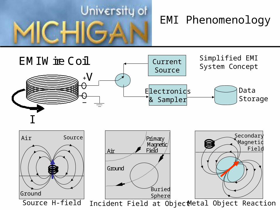
EMI Phenomenology

Air

Ground

Primary MagneticField

BuriedSphere

CurrentSource

Electronics& Sampler

DataStorage

I

V+

_

EMI Wire Coil

I

V+

_

EMI Wire Coil Simplified EMISystem Concept

Air

Ground

Source

SecondaryMagnetic

Field

Source H-field Incident Field at Object Metal Object Reaction

duruJeum

zyxH hd

u

z )(2

),,( 0)(

0 21

30

021

duruJeum

zyxH hd

u

r )(2

),,( 1)(

0 21

210

021

)( 111122

1 ju

)( 222222

2 ju

Air

Ground

Source

Source H-field

(x,y,-d)

(x,y,h)

EMI Phenomenology

),,(),,,(2 03

ssszssz zyxHaPam

),,(),,,(2 03

sssrssr zyxHaPam

))sinh()cosh()(sinh())cosh()(sinh(

))sinh()cosh()(sinh())cosh()(sinh(2),,,(

20

20

s

sss aP

)( ssia

Metal Object Reaction

SecondaryMagnetic

Field

pr

pz

duruJeum

zyxH hz

u

zzz )(

2),,( 0

)(

0 21

321

duruJeum

zyxH hz

u

rrz )(

2),,( 1

)(

0 21

21 21

EMI Phenomenology

* Model assumes a solid spherical target.

zzzzxxzx pHHpHHv 00

InducedMagnetic

Sources

px

pz

* Model no longer assumes a solid spherical target.

H0x – Horizontal magnetic field at the center of the target produced by the source magnetic dipole.

Hxz – Vertical magnetic field at the receive coil produced by the horizontal induced magnetic dipole.

H0z – Vertical magnetic field at the center of the target produced by the source magnetic dipole.

Hzz – Vertical magnetic field at the receive coil produced by the vertical induced magnetic dipole.

z

x

p

p TargetMagneticPolarizabilityVector

EMI Phenomenology

Vertical Dipole Horizontal Dipole

Physics DerivedBasis Functions

-1.5 -1 -0.5 0 0.5 1 1.5

-0.4

-0.2

0

0.2

0.4

0.6

Sample Location [m]

Vol

tage

Res

pons

e

-1.5 -1 -0.5 0 0.5 1 1.5

-0.4

-0.2

0

0.2

0.4

0.6

Sample Location [m]

Vol

tage

Res

pons

e

The Basis Function

TheW Basis Function

• The vertical dipole produces the basis.

• The horizontal dipole produces the W basis.

)()( xbWxaxs dd

Physics DerivedBasis Functions

d – depth of buried object

a – Polarizability of object in Z-direction.

b – Polarizability of object in X-direction.

• The spatial signal is composed of the (x) and W(x) basis functions.

• The basis functions are parameterized by depth.

• Any object at the same depth will have the same basis.

• The object’s shape affects the weighting coeffs “a” and “b”.

Sphere at 0.0m

All objects simulated at 0.25m depth.

• These 3 signals come from identical spheres at different depths.

Canonical Depths

-1.5 -1 -0.5 0 0.5 1 1.5-1

-0.5

0

0.5

1

1.5x 10

-3

Sample Location [m]

Vol

tage

Res

pons

e

Sphere at 1.0m

Sphere at 0.25m Sphere at 1.0m

-1.5 -1 -0.5 0 0.5 1 1.5-0.1

-0.05

0

0.05

0.1

0.15

0.2

0.25

Sample Location [m]

Vol

tage

Res

pons

e

Sphere at 0.25m

-1.5 -1 -0.5 0 0.5 1 1.5-4

-2

0

2

4

6

8

Sample Location [m]

Vol

tage

Res

pons

e

Sphere at 0.0m

Canonical Depths

-1.5 -1 -0.5 0 0.5 1 1.5-2

-1

0

1

2

3

4

5

Sample Location [m]

Vol

tage

Res

pons

e

Sphere at 0.0m

a Component

bW Component-1.5 -1 -0.5 0 0.5 1 1.5

-0.04

-0.02

0

0.02

0.04

0.06

0.08

0.1

0.12

Sample Location [m]

Vol

tage

Res

pons

e

Sphere at 0.25m

a Component

bW Component-1.5 -1 -0.5 0 0.5 1 1.5

-2

-1

0

1

2

3

4

5

6

x 10-4

Sample Location [m]V

olta

ge R

espo

nse

Sphere at 1.0m

a Component

bW Component

Sphere at 0.0m

• These 3 signals come from identical spheres at different depths.

Sphere at 0.25m Sphere at 1.0m

d

Wd

2D SignalSubspace

HigherDimensional

Space

2D PlaneSpanned byd and Wd

• The natural d and Wd bases are non-orthogonal. • An interesting fact is that thed and Wd bases form an angle of 62° regardless of object depth d.

• All metal objects at this depth will exist in this signal subspace.

d

Wd

62°

Subspaces for Objects at

Different Depths

• The bases of objects at a second depth, d2 and Wd2, span a second plane that is non-orthogonal to the plane spanned by the first depth bases, d1 and Wd1.

d1

Wd1

d2

Wd2

First Depth Subspace

SecondDepthSubspace

Sphere Cylinder Flat Plate

-1.5 -1 -0.5 0 0.5 1 1.5

-0.4

-0.2

0

0.2

0.4

0.6

Sample Location [m]V

olta

ge R

espo

nse

Flat Plate

-1.5 -1 -0.5 0 0.5 1 1.5

-0.4

-0.2

0

0.2

0.4

0.6

Sample Location [m]

Vol

tage

Res

pons

e

Cylinder

-1.5 -1 -0.5 0 0.5 1 1.5

-0.4

-0.2

0

0.2

0.4

0.6

Sample Location [m]

Vol

tage

Res

pons

e

Sphere

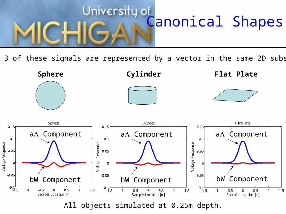
All objects simulated at 0.25m depth.

• All 3 of these signals are represented by a vector in the same 2D subspace.

Canonical Shapes

Sphere Cylinder Flat Plate

All objects simulated at 0.25m depth.

• All 3 of these signals are represented by a vector in the same 2D subspace.

Canonical Shapes

-1.5 -1 -0.5 0 0.5 1 1.5-0.1

-0.05

0

0.05

0.1

0.15

Sample Location [m]

Vol

tage

Res

pons

e

Sphere

-1.5 -1 -0.5 0 0.5 1 1.5-0.1

-0.05

0

0.05

0.1

0.15

Sample Location [m]

Vol

tage

Res

pons

e

Cylinder

-1.5 -1 -0.5 0 0.5 1 1.5-0.1

-0.05

0

0.05

0.1

0.15

Sample Location [m]V

olta

ge R

espo

nse

Flat Plate

a Component a Component a Component

bW Component bW Component bW Component

Effect of Object Shape, Size, and Content

d

Wd

62°

45°-Sphere

30°-Cylinder

10°-Flat Plate

Larger or MoreConductive Sphere

Larger or MoreConductive Cylinder

Larger or MoreConductive Flat Plate

  a b angle

sphere 1 1 45°

cylinder 1 0.5 30°

flat plate 1 0.176 10°

2D Subspace forObjects at Depth “d”

• The object’s polarizability (the a and b coeffs) determines the angle of the signal in the 2D subspace.

• Increasing the object’s size increases the weightings, a and b.

• More conductive metal also increases the weightings, a and b.

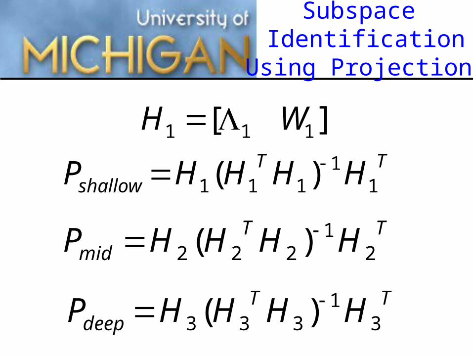
TTshallow HHHHP 1

1111 )(

][ 111 WH

TTmid HHHHP 2

1222 )(

TTdeep HHHHP 3

1333 )(

Subspace Identification

Using Projections

-1.5 -1 -0.5 0 0.5 1 1.5

-0.4

-0.3

-0.2

-0.1

0

0.1

0.2

0.3

0.4

0.5

-1.5 -1 -0.5 0 0.5 1 1.5-0.15

-0.1

-0.05

0

0.05

0.1

0.15

0.2

0.25

0.3

-1.5 -1 -0.5 0 0.5 1 1.5-0.3

-0.2

-0.1

0

0.1

0.2

0.3

0.4

DeepSphere

DeepSphere

DeepSphere

Subspace IdentificationPerformance

Table 3a: Norm After Projection into Subspace (No Noise)

  Spheres Flat Plates Cylinders

  Shallow Mid Deep Shallow Mid Deep Shallow Mid Deep

Shallow 1.00 0.80 0.79 1.00 0.99 0.93 1.00 0.95 0.94

Mid 0.69 1.00 0.79 0.92 1.00 0.99 0.81 1.00 0.96

Deep 0.31 0.51 1.00 0.63 0.85 1.00 0.35 0.71 1.00

Table 3b: Norm After Projection into Subspace (Noise Var: 0.01)

  Spheres Flat Plates Cylinders

  Shallow Mid Deep Shallow Mid Deep Shallow Mid Deep

Shallow 0.98 0.75 0.73 0.98 0.97 0.92 0.99 0.93 0.92

Mid 0.66 0.97 0.71 0.92 0.98 0.97 0.84 0.98 0.94

Deep 0.32 0.54 0.93 0.64 0.83 0.98 0.38 0.72 0.96

Table 3c: Norm After Projection into Subspace (Noise Var: 0.05)

  Spheres Flat Plates Cylinders

  Shallow Mid Deep Shallow Mid Deep Shallow Mid Deep

Shallow 0.70 0.49 0.39 0.84 0.81 0.58 0.73 0.68 0.57

Mid 0.41 0.59 0.39 0.79 0.80 0.62 0.64 0.71 0.55

Deep 0.04 0.39 0.44 0.58 0.67 0.65 0.28 0.30 0.55

-1.5 -1 -0.5 0 0.5 1 1.5-0.3

-0.2

-0.1

0

0.1

0.2

0.3

0.4

0.5

-1.5 -1 -0.5 0 0.5 1 1.5-0.3

-0.2

-0.1

0

0.1

0.2

0.3

0.4

0.5

-1.5 -1 -0.5 0 0.5 1 1.5-0.3

-0.2

-0.1

0

0.1

0.2

0.3

0.4

0.5

MidDepthSphere

MidDepthSphere

MidDepthSphere

600Hz to 60kHz

New EMIModality

Georgia Tech EMI

-1.5 -1 -0.5 0 0.5 1 1.5-0.2

-0.15

-0.1

-0.05

0

0.05

0.1

0.15

0.2

Sample Location [m]

Vol

tage

Res

pons

e

1kHzrealimag*10

-1.5 -1 -0.5 0 0.5 1 1.5-0.2

-0.15

-0.1

-0.05

0

0.05

0.1

0.15

0.2

Sample Location [m]

Vol

tage

Res

pons

e

10kHzrealimag*10

-1.5 -1 -0.5 0 0.5 1 1.5-0.2

-0.15

-0.1

-0.05

0

0.05

0.1

0.15

0.2

Sample Location [m]

Vol

tage

Res

pons

e

20kHzrealimag*10

-1.5 -1 -0.5 0 0.5 1 1.5-0.2

-0.15

-0.1

-0.05

0

0.05

0.1

0.15

0.2

Sample Location [m]

Vol

tage

Res

pons

e

30kHzrealimag*10

-1.5 -1 -0.5 0 0.5 1 1.5-0.2

-0.15

-0.1

-0.05

0

0.05

0.1

0.15

0.2

Sample Location [m]

Vol

tage

Res

pons

e

40kHzrealimag*10

-1.5 -1 -0.5 0 0.5 1 1.5-0.2

-0.15

-0.1

-0.05

0

0.05

0.1

0.15

0.2

Sample Location [m]

Vol

tage

Res

pons

e

50kHzrealimag*10

-1.5 -1 -0.5 0 0.5 1 1.5-0.2

-0.15

-0.1

-0.05

0

0.05

0.1

0.15

0.2

Sample Location [m]

Vol

tage

Res

pons

e

60kHzrealimag*10

Fast 3D Blind Deconvolution of Even Point Spread Functions

Andrew Yagle and Siddharth ShahThe University of Michigan, Ann Arbor

Part II of thisPresentation

Motivation

Many blind deconvolutionalgorithms need an initial PSF estimate

Can be tedious and problematic to measure PSF accurately

Blind Deconvolution(Don’t need PSF)BUT

But Blind Deconvolution algorithms tend to be slow !Also many still need initial PSF estimate

What we need

A fast algorithm that performs blind deconvolution

We will show:

An algorithm that performs blind deconvolution that is

• Fast

• Parallelizable

• A linear algebraic formulation

• Non iterative (at least for the Least Squares solution)

Assumptions

1. Point Spread Function or

PSF h(x,y,z) is even in 3-D.Reasonable in optics. PSFsare symmetric in x, y, and z.Hence h(x,y,z) = h(-x,-y,-z)

2. We know the PSF or image support size.

3. Image has compact support.

Potential Problem: Asymmetric PSFs due to optical aberrations

Can these be solved too ? YES (later)

Formulation

y(i1,i2,i3) = h(i1,i2,i3) *** u(i1,i2,i3) + n(i1,i2,i3)

DATA PSF OBJECT NOISE

where u(i1,i2,i3) ≠ 0 for 0 ≤ i1,i2,i3 ≤ M-1 h(i1,i2,i3) ≠ 0 for 0 ≤ i1,i2,i3 ≤ L-1 y(i1,i2,i3) ≠ 0 for 0 ≤ i1,i2,i3 ≤ N-1 N=L+M-1

h(i1,i2,i3) = h(L-i1,L-i2,L-i3) (even PSF)n(i1,i2,i3) is zero mean white Gaussian noise.

PROBLEMGiven only data y(i1,i2,i3) reconstruct the object u(i1,i2,i3)and the PSF h(i1,i2,i3)

1-D Solution

)()1

()1

()(

)()1

()()()(

transformz Taking

even is ),()()(

1 zUz

Yzz

UzzY

zUz

HzzUzHzY

h(n)nunhny

NM

L

Equating coefficients, we get the following matrix

0

0

)1(

)0(

)0(

)1(

)0(*00)1(0

)1(*)2(

)2(*)1(

00)1(*00)0(

Mu

u

u

Mu

yNy

yNy

Nyy

Nyy

Toeplitz Structure

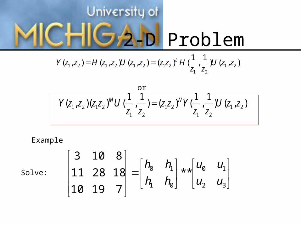
2-D Problem

),()1

,1

()(),(),(),( 2121

21212121 zzUzz

HzzzzUzzHzzY L

),()1

,1

()()1

,1

()(),( 2121

2121

2121 zzUzz

Yzzzz

UzzzzY NM

or

Example

Solve:

32

10

01

10 **

71910

182811

8103

uu

uu

hh

hh

2-D Example

0

0

0

0

0

0

0

0

0

0

0

0

0

0

0

0

100008000

11100018800

3110071800

03000700

19010010080

281911102810188

10283111928718

0100301907

7019030100

18728191132810

818102810111928

08010010019

00700030

0018700113

00818001011

000800010

1

3

0

2

2

0

3

1

u

u

u

u

u

u

u

u

Solution

75

43

32

10

uu

uu

Toeplitz Block Toeplitz structure

Size of matrix(2M + L- 2)2 X (2M2)

3-D Solution

),,()1

,1

,1

()()1

,1

,1

()(),,( 321321

321321

321321 zzzUzzz

Yzzzzzz

UzzzzzzY NM

Equating coefficients we would get a doubly nested Toeplitz matrix

Matrix size: (2M + L-2)3 X (2M)3

Q: So we have solved the 3D problem ?A: Not quite !! If M=5 and L=3 then the matrix size is 4913 X1024

It will be intractable to use this method “as is” in 3D !

FourierDecomposition

)1

,1

,1

())(,,()1

,1

,1

())(,,(

Then

,,Let

313131

313131

/2/2/2

zyzYzyzzyzU

zyzUzyzzyzY

ezeyex

k

Nkk

k

Mkk

Mkjk

Mkjk

Mkjk

)*

1,,

*

1())(,,()

*

1,,

*

1(*))(,,(

313131

313131 z

yz

YzyzzyzUz

yz

UzyzzyzY kN

kkkM

kk

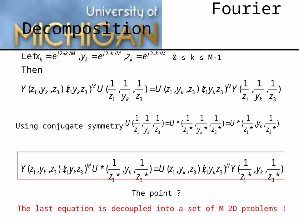
Using conjugate symmetry )*

1,,

*

1(*)

*

1,

*

1,

*

1(*)

1,

1,

1(

313131 zy

zU

zyzU

zyzU k

kk

The point ?

The last equation is decoupled into a set of M 2D problems !

0 ≤ k ≤ M-1

2-D to 1-D

So we broke down a huge 3D problem to M simpler 2D problems

What next ?

Substitute for xk in each 2D problem and you would get M 1D problems in z

To summarize

We broke up a large 3D problem into M2 1D problems

)*

1,,())(,,()

*

1,,(*))(,,(

333

333 z

yxYzyxzyxUz

yxUzyxzyxY kkN

kkkkkkM

kkkk

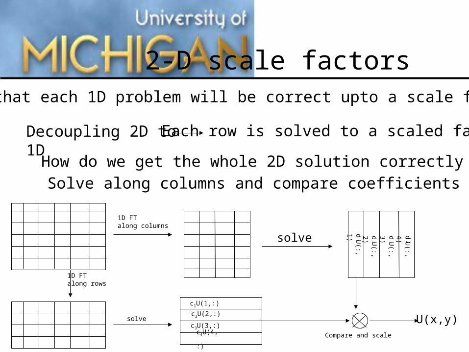
2-D scale factors

Note that each 1D problem will be correct upto a scale factor.

Decoupling 2D to 1D Each row is solved to a scaled factor.

How do we get the whole 2D solution correctly ?

Solve along columns and compare coefficients

1D FTalong columns

1D FTalong rows

solve

c1U(1,:) c2U(2,:) c3U(3,:) c4U(4,:)

solve d1U

(:,1) d

2U(:,

2) d3U

(:,3)

d4U

(:,4)

Compare and scale

U(x,y)

3-D scale factors

We just learned how a 2D problem could be correctly scaled

Decouple 3D to 2DSolve 3D Decouple 2D to 1D Solve 1D

Scale 1D SolnsScale 2D Solns 2D solutions

c1

c2

d1 d2

U(x,y,z)Decouple along z

Solve 2D problems

Solve 2D problems

Decouple along x

Compareand scale

2D problems

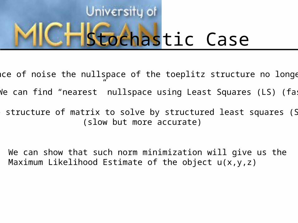
Stochastic Case

In presence of noise the nullspace of the toeplitz structure no longer exists.

We can find “nearest” nullspace using Least Squares (LS) (fast)

Can use structure of matrix to solve by structured least squares (STLS)(slow but more accurate)

We can show that such norm minimization will give us the Maximum Likelihood Estimate of the object u(x,y,z)

Simulations

Synthetic bead image (30X30X30), (3X3X3) PSF, no noise

Stochastic case: STLN vs. LS

Least Squares v/s STLN comparison

Least squares does well at highSNRs but at low and mediumSNRS STLN is better.

7X7X7 image. 3X3X3 PSF. 50 iterations per SNR

Comparison with Lucy Richardson

SNR SNR

MSETime

Our algorithm gave a lower MSE. In LRFinal accuracy even in absence of noisedepends on initial PSF estimate.

Our algorithm need only a fixed amountof time to solve independent of the SNR.LR needs more time and time to solve depends on the SNR.