–1–

Deconvolution Signal ModelsDeconvolution Signal Models

• Simple or Fixed-shape regression (previous talks): We fixed the shape of the HRF — amplitude varies Used -stim_times to generate the signal model from the stimulus timing

Found the amplitude of the signal model in each voxel — solution to the set of linear equations = weights

• Deconvolution or Variable-shape regression (now): We allow the shape of the HRF to vary in each voxel, for each stimulus class

Appropriate when you don’t want to over-constrain the solution by assuming an HRF shape

Caveat : need to have enough time points during the HRF in order to resolve its shape

–2–

Deconvolution: Pros & Cons (+ & –)+ Letting HRF shape varies allows for subject and regional variability in hemodynamics

+ Can test HRF estimate for different shapes (e.g., are later time points more “active” than earlier?)

– Need to estimate more parameters for each stimulus class than a fixed-shape model (e.g., 4-15 vs. 1 parameter = amplitude of HRF)

– Which means you need more data to get the same statistical power (assuming that the fixed-shape model you would otherwise use was in fact “correct”)

– Freedom to get any shape in HRF results can give weird shapes that are difficult to interpret

–3– Expressing HRF via Regression Unknowns

• The tool for expressing an unknown function as a finite set of numbers that can be fit via linear regression is an expansion in basis functions

The basis functions q(t ) & expansion order p are knowno Larger p more complex shapes & more parameters

The unknowns to be found (in each voxel) comprises the set of weights q for each q(t )

• weights appear only by multiplying known values, and HRF only appears in signal model by linear convolution (addition) with known stimulus timing• Resulting signal model still solvable by linear regression

h(t) =0 0 (t) + 1 1(t) + 2 2 (t) +L = q q(t)

q=0

q=p

∑

–4–

• Need to describe HRF shape and magnitude with a finite number of parameters And allow for calculation of h(t ) at any arbitrary point in time after the stimulus times:

• Simplest set of such functions are tent functions Also known as “piecewise linear splines”

T (x) =1− x for −1< x<10 for x >1

⎧⎨⎩

time

h

t = 0 t =TR t = 2TR t = 3TR t = 4TR t = 5TR

Tt −3⋅TR2 ⋅TR

⎛⎝⎜

⎞⎠⎟

3dDeconvolve with “Tent Functions”

rn = h(tn −τ k)k=1

K∑ =sum of HRF copies

–5–

Tent Functions = Linear Interpolation• Expansion of HRF in a set of spaced-apart tent functions is the same as linear interpolation between “knots”

• Tent function parameters are also easily interpreted as function values (e.g., 2 = response at time t = 2L after stim)

• User must decide on relationship of tent function grid spacing L and time grid spacing TR (usually would choose L TR)

• In 3dDeconvolve: specify duration of HRF and number of parameters (details shown a few slides ahead)

h(t)=0 ⋅T

tL

⎛⎝⎜

⎞⎠⎟+1 ⋅T

t−LL

⎛⎝⎜

⎞⎠⎟+2 ⋅T

t−2⋅LL

⎛⎝⎜

⎞⎠⎟+3 ⋅T

t−3⋅LL

⎛⎝⎜

⎞⎠⎟+L

time

0

1

2 3

4

L 2L 3L 4L 5L0

5

N.B.: 5 intervals = 6 weights

“knot” times

h

A

–6–

Tent Functions: Average Signal Change• For input to group analysis, usually want to compute average signal change Over entire duration of HRF (usual)

Over a sub-interval of the HRF duration (sometimes)

• In previous slide, with 6 weights, average signal change is

1/2 0 + 1 + 2 + 3 + 4 + 1/2 5

• First and last weights are scaled by half since they only

affect half as much of the duration of the response

• In practice, may want to use 00 since immediate post-

stimulus response is not neuro-hemodynamically relevant

• All weights (for each stimulus class) are output into the “bucket” dataset produced by 3dDeconvolve

• Can then be combined into a single number using 3dcalc

–7–

Deconvolution and Collinearity• Regular stimulus timing can lead to collinearity!

time

0 1 2 3 4 5

0 1 2 3 4 5

0 1 2 3

0

+4

1

+5

2 3 0

+4

1

+5

2 3 0

+4

1

+5

2 3Equationsat each data time point:Cannot tell0 from 4,or 1 from 5

0 1 2 3 4 5

HRF fromstim #1

stim #1

Tail of HRFfrom #1 overlapshead of HRFfrom #2, etc

A

–8–

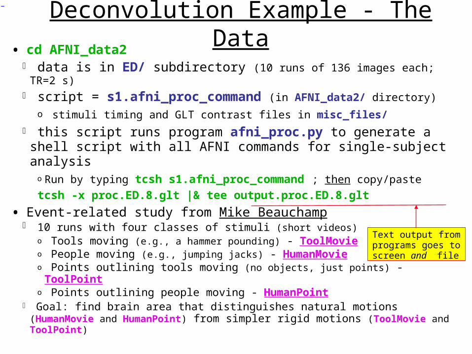
Deconvolution Example - The Data• cd AFNI_data2

data is in ED/ subdirectory (10 runs of 136 images each; TR=2 s) script = s1.afni_proc_command (in AFNI_data2/ directory)

o stimuli timing and GLT contrast files in misc_files/

this script runs program afni_proc.py to generate a shell script with all AFNI commands for single-subject analysis

o Run by typing tcsh s1.afni_proc_command ; then copy/paste

tcsh -x proc.ED.8.glt |& tee output.proc.ED.8.glt

• Event-related study from Mike Beauchamp 10 runs with four classes of stimuli (short videos)

o Tools moving (e.g., a hammer pounding) - ToolMovieo People moving (e.g., jumping jacks) - HumanMovieo Points outlining tools moving (no objects, just points) - ToolPointo Points outlining people moving - HumanPoint

Goal: find brain area that distinguishes natural motions (HumanMovie and HumanPoint) from simpler rigid motions (ToolMovie and ToolPoint)

Text output fromprograms goes toscreen and file

–9–

Master Script for Data Analysisafni_proc.py \ -dsets ED/ED_r??+orig.HEAD \ -subj_id ED.8.glt \ -copy_anat ED/EDspgr \ -tcat_remove_first_trs 2 \ -volreg_align_to first \ -regress_stim_times misc_files/stim_times.*.1D \ -regress_stim_labels ToolMovie HumanMovie \ ToolPoint HumanPoint \ -regress_basis 'TENT(0,14,8)' \ -regress_opts_3dD \ -gltsym ../misc_files/glt1.txt -glt_label 1 FullF \ -gltsym ../misc_files/glt2.txt -glt_label 2 HvsT \ -gltsym ../misc_files/glt3.txt -glt_label 3 MvsP \ -gltsym ../misc_files/glt4.txt -glt_label 4 HMvsHP \ -gltsym ../misc_files/glt5.txt -glt_label 5 TMvsTP \ -gltsym ../misc_files/glt6.txt -glt_label 6 HPvsTP \ -gltsym ../misc_files/glt7.txt -glt_label 7 HMvsTM

• Master script program• 10 input datasets• Set output filenames• Copy anat to output dir• Discard first 2 TRs• Where to align all EPIs• Stimulus timing files (4)• Stimulus labels

• HRF model• Specifies that next

lines are options to be passed to 3dDeconvolve directly (in this case, the GLTs we want computed)

This script generates file proc.ED.8.glt (180 lines), which contains all the AFNI commands to produce analysis results

into directory ED.8.glt.results/ (148 files)

–10–

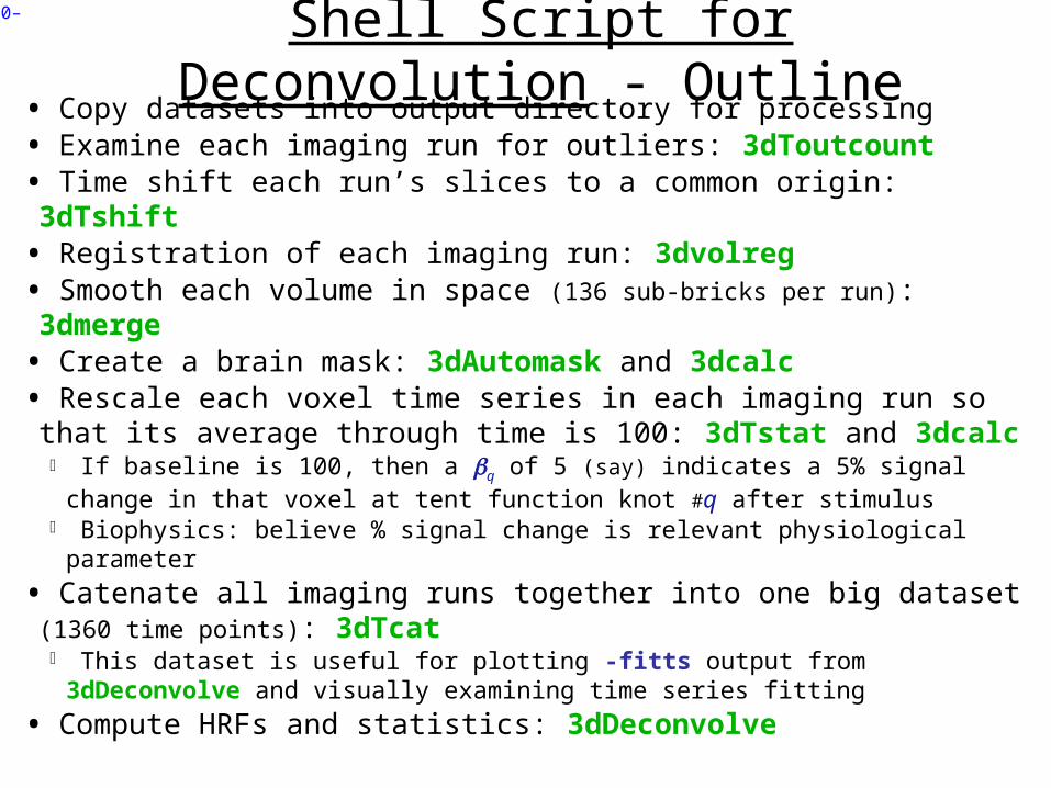
Shell Script for Deconvolution - Outline• Copy datasets into output directory for processing• Examine each imaging run for outliers: 3dToutcount• Time shift each run’s slices to a common origin: 3dTshift• Registration of each imaging run: 3dvolreg• Smooth each volume in space (136 sub-bricks per run): 3dmerge• Create a brain mask: 3dAutomask and 3dcalc• Rescale each voxel time series in each imaging run so that its average through time is 100: 3dTstat and 3dcalc

If baseline is 100, then a q of 5 (say) indicates a 5% signal change in that voxel at tent function knot #q after stimulus

Biophysics: believe % signal change is relevant physiological parameter

• Catenate all imaging runs together into one big dataset (1360

time points): 3dTcat This dataset is useful for plotting -fitts output from 3dDeconvolve

and visually examining time series fitting

• Compute HRFs and statistics: 3dDeconvolve

–11–

Script - 3dToutcount# set list of runsset runs = (`count -digits 2 1 10`)# run 3dToutcount for each runforeach run ( $runs ) 3dToutcount -automask pb00.$subj.r$run.tcat+orig > outcount_r$run.1Dend

Via 1dplot outcount_r??.1D3dToutcount searches for “outliers” in data time series;You may want to examine noticeable runs & time points

–12–

Script - 3dTshift# run 3dTshift for each runforeach run ( $runs ) 3dTshift -tzero 0 -quintic -prefix pb01.$subj.r$run.tshift \ pb00.$subj.r$run.tcat+origend

• Produces new datasets where each time series has been shifted to have the same time origin• -tzero 0 means that all data time series are interpolated to match the time offset of the first slice

• Which is what the slice timing files usually refer to• Quintic (5th order) polynomial interpolation is used

• 3dDeconvolve will be run on time-shifted datasets• This is mostly important for Event-Related FMRI studies, where the response to the stimulus is briefer than for Block designs

• (Because the stimulus is briefer)

• Being a little off in the stimulus timing in a Block design is not likely to matter much

–13–

Script - 3dvolreg# align each dset to the base volumeforeach run ( $runs ) 3dvolreg -verbose -zpad 1 -base pb01.$subj.r01.tshift+orig'[0]' \ -1Dfile dfile.r$run.1D -prefix pb02.$subj.r$run.volreg \ pb01.$subj.r$run.tshift+origend

• Produces new datasets where each volume (one time point) has been aligned (registered) to the #0 time point in the #1 dataset• Movement parameters are saved into files dfile.r$run.1D

• Will be used as extra regressors in 3dDeconvolve to reduce motion artifacts

1dplot -volreg dfile.rall.1D• Shows movement parameters for all runs (1360 time points) in degrees and millimeters• Important to look at this graph!• Excessive movement can make an imaging run useless — 3dvolreg won’t be able to compensate

• Pay attention to scale of movements: more than about 2 voxel sizes in a short time interval is usually bad

–14–

Script - 3dmerge# blur each volumeforeach run ( $runs ) 3dmerge -1blur_fwhm 4 -doall -prefix pb03.$subj.r$run.blur \ pb02.$subj.r$run.volreg+origend

• Why Blur? Reduce noise by averaging neighboring voxels time series

• WhiteWhite curve = Data: unsmoothed• YellowYellow curve = Model fit (R2 = 0.50)• GreenGreen curve = Stimulus timing

This is an extremely good fit for ER FMRI data!

–15–

Why Blur? - 2 • fMRI activations are (usually) blob-

ish (several voxels across)

• Averaging neighbors will also reduce the fiendish multiple comparisons problem Number of independent “resels” will be smaller than

number of voxels (e.g., 2000 vs. 20000)

• Why not just acquire at lower resolution? To avoid averaging across brain/non-brain interfaces To project onto surface models

• Amount to blur is specified as FWHM (Full Width at Half Maximum) of spatial averaging filter (4 mm in script)

–16–

Script - 3dAutomask# create 'full_mask' dataset (union mask)foreach run ( $runs ) 3dAutomask -dilate 1 -prefix rm.mask_r$run pb03.$subj.r$run.blur+origend# get mean and compare it to 0 for taking 'union'3dMean -datum short -prefix rm.mean rm.mask*.HEAD3dcalc -a rm.mean+orig -expr 'ispositive(a-0)' -prefix full_mask.$subj

• 3dAutomask creates a mask of contiguous high-intensity voxels (with

some hole-filling) from each imaging run separately• 3dMean and 3dcalc are used to create a mask that is the union of all the individual run masks• 3dDeconvolve analysis will be limited to voxels in this mask

• Will run faster, since less data to process

–17–

Script - Scaling# scale each voxel time series to have a mean of 100# (subject to maximum value of 200)foreach run ( $runs ) 3dTstat -prefix rm.mean_r$run pb03.$subj.r$run.blur+orig 3dcalc -a pb03.$subj.r$run.blur+orig -b rm.mean_r$run+orig \ -c full_mask.$subj+orig \ -expr 'c * min(200, a/b*100)' -prefix pb04.$subj.r$run.scaleend

• 3dTstat calculates the mean (through time) of each voxel’s time series data• For voxels in the mask, each data point is scaled (multiplied) using 3dcalc so that it’s time series will have mean = 100• If an HRF regressor has max amplitude

= 1, then its coefficient will represent the percent signal change (from the mean) due to that part of the signal model• Scaled images are very boring

• No spatial contrast by design!• Graphs have common baseline now

–18–

Script - 3dDeconvolve3dDeconvolve -input pb04.$subj.r??.scale+orig.HEAD -polort 2 \ -mask full_mask.$subj+orig -basis_normall 1 -num_stimts 10 \ -stim_times 1 stimuli/stim_times.01.1D 'TENT(0,14,8)' \ -stim_label 1 ToolMovie \ -stim_times 2 stimuli/stim_times.02.1D 'TENT(0,14,8)' \ -stim_label 2 HumanMovie \ -stim_times 3 stimuli/stim_times.03.1D 'TENT(0,14,8)' \ -stim_label 3 ToolPoint \ -stim_times 4 stimuli/stim_times.04.1D 'TENT(0,14,8)' \ -stim_label 4 HumanPoint \ -stim_file 5 dfile.rall.1D'[0]' -stim_base 5 -stim_label 5 roll \ -stim_file 6 dfile.rall.1D'[1]' -stim_base 6 -stim_label 6 pitch \ -stim_file 7 dfile.rall.1D'[2]' -stim_base 7 -stim_label 7 yaw \ -stim_file 8 dfile.rall.1D'[3]' -stim_base 8 -stim_label 8 dS \ -stim_file 9 dfile.rall.1D'[4]' -stim_base 9 -stim_label 9 dL \ -stim_file 10 dfile.rall.1D'[5]' -stim_base 10 -stim_label 10 dP \ -iresp 1 iresp_ToolMovie.$subj -iresp 2 iresp_HumanMovie.$subj \ -iresp 3 iresp_ToolPoint.$subj -iresp 4 iresp_HumanPoint.$subj \ -gltsym ../misc_files/glt1.txt -glt_label 1 FullF \ -gltsym ../misc_files/glt2.txt -glt_label 2 HvsT \ -gltsym ../misc_files/glt3.txt -glt_label 3 MvsP \ -gltsym ../misc_files/glt4.txt -glt_label 4 HMvsHP \ -gltsym ../misc_files/glt5.txt -glt_label 5 TMvsTP \ -gltsym ../misc_files/glt6.txt -glt_label 6 HPvsTP \ -gltsym ../misc_files/glt7.txt -glt_label 7 HMvsTM \ -fout -tout -full_first -x1D Xmat.x1D -fitts fitts.$subj -bucket stats.$subj

4 stim types

motion params

GLTs

HRF outputs

–19–

Results: Humans vs. Tools• Color overlay: HvsT GLT contrast

• Blue (upper) graphs: Human HRFs

• Red (lower) graphs: Tool HRFs

–20–

Script - X Matrix

Via 1grayplot -sep Xmat.x1D

–21–

Script - Random Comments•-polort 2

Sets baseline (detrending) to use quadratic polynomials—in each run

•-mask full_mask.$subj+origProcess only the voxels that are nonzero in this mask dataset

•-basis_normall 1Make sure that the basis functions used in the HRF expansion all

have maximum magnitude=1•-stim_times 1 stimuli/stim_times.01.1D 'TENT(0,14,8)' -stim_label 1 ToolMovie

The HRF model for the ToolMovie stimuli starts at 0 s after each stimulus, lasts for 14 s, and has 8 basis tent functions

o Which have knots spaced 14/(8-1) = 2 s apart)•-iresp 1 iresp_ToolMovie.$subj

The HRF model for the ToolMovie stimuli is output into dataset iresp_ToolMovie.ED.8.glt+orig

–22–

Script - GLTs• -gltsym ../misc_files/glt2.txt -glt_label 2 HvsT

File ../misc_files/glt2.txt contains 1 line of text:o -ToolMovie +HumanMovie -ToolPoint +HumanPointo This is the “Humans vs. Tools” HvsT contrast shown on Results slide

• This GLT means to take all 8 coefficients for each stimulus class and combine them with additions and subtractions as ordered:

• This test is looking at the integrated (summed) response to the “Human” stimuli and subtracting it from the integrated response to the “Tool” stimuli

•Combining subsets of the weights is also possible with -gltsym :• +HumanMovie[2..6] -HumanPoint[2..6]• This GLT would add up just the #2,3,4,5, & 6 weights for one

type of stimulus and subtract the sum of the #2,3,4,5, & 6 weights for another type of stimulus

o And also produce F- and t-statistics for this linear combination

LC =−0TM −L −7

TM +0HM +L +7

HM −0TP −L −7

TP +0HP +L +7

HP

–23–

Script - Multi-Row GLTs• GLTs presented up to now have had one row

Testing if some linear combination of weights is nonzero; test statistic is t or F (F =t

2 when testing a single number) Testing if the X matrix columns, when added together to form one column as specified by the GLT (+ and –), explain a significant fraction of the data time series (equivalent to above)

• Can also do a single test to see if several different combinations of weights are all zero

-gltsym ../misc_files/glt1.txt -glt_label 1 FullF

Tests if any of the stimulus classes have nonzero integrated HRF (each name means “add up those weights”) : DOF= (4,1292)

Different than the default “Full F-stat” produced by 3dDeconvolve, which tests if any of the individual weights are nonzero: DOF= (32,1292)

+ToolMovie+HumanMovie+ToolPoint+HumanPoint

4 rows

–24–

Two Possible Formats for -stim_times• A single column of numbers (GLOBAL times)

One stimulus time per row Times are relative to first image in dataset being at t = 0 May not be simplest to use if multiple runs are catenated

• One row for each run within a catenated dataset (LOCAL times)

Each time in j th row is relative to start of run #j being t = 0 If some run has NO stimuli in the given class, just put a single “*” in that row as a filler

o Different numbers of stimuli per run are OKo At least one row must have more than 1 time (so that the LOCAL type of timing file can be told from the GLOBAL)

• Two methods are available because of users’ diverse needs N.B.: if you chop first few images off the start of each run, the inputs to -stim_times must be adjusted accordingly!

4.79.611.819.4

4.7 9.6 11.8 19.4*8.3 10.6