Overview of Inference Algorithms Overview of Inference Algorithms for Bayesian Networksfor Bayesian Networks

Wei Sun, PhDWei Sun, PhD

Assistant Research ProfessorAssistant Research Professor

SEOR Dept. & C4I CenterSEOR Dept. & C4I Center

George Mason University, 2009George Mason University, 2009

2

Outline

Bayesian network and its properties

Probabilistic inference for Bayesian networks

Inference algorithm overview

Junction tree algorithm review

Current research

3

Definition of BN

A Bayesian network is a directed, acyclic graph consisting of nodes and arcs: Nodes: variables Arcs: probabilistic dependence relationships. Parameters: for each node, there is a conditional probability distribution

(CPD).

CPD of Xi: P(Xi|Pa(Xi)) where Pa(Xi) represents all parents of Xi

Discrete: CPD is typically represented as a table, also called CPT. Continuous: CPD involves functions, such as P(Xi|Pa(Xi)) = f(Pa(Xi), w),

where w is a random noise.

Joint distribution of variables in BN is

4

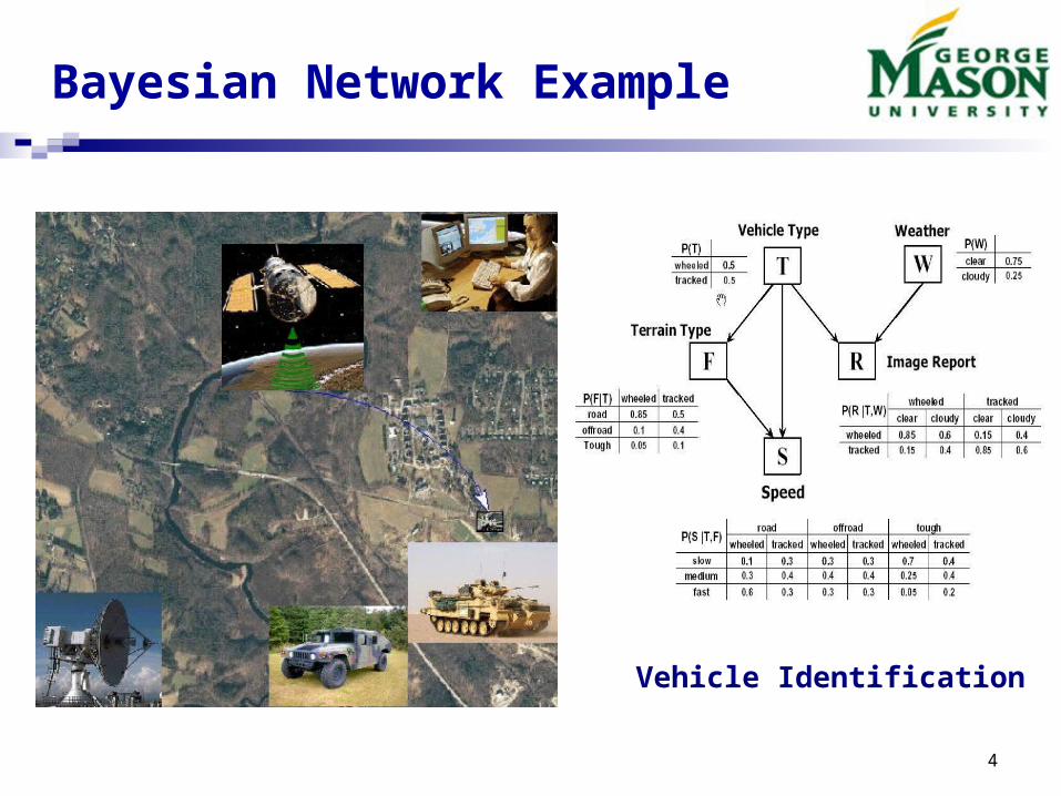
Bayesian Network Example

Vehicle Identification

5

Probabilistic Inference in BN

Task: find the posterior distributions of query nodes given evidence. Bayes’ Rule:

Both exact and approximate inference using BNs are NP-hard. Tractable inference algorithms exist only for special classes of BNs.

6

Classify BNs by Network Structure

Multiply - connected networksSingly-connected networks (a.k.a. polytree)

7

Classify BNs by Node Types

Node types Discrete: conditional probability

distribution is usually represented as a table.

Continuous: Gaussian or non-Gaussian distribution; conditional probability distribution is specified using functions:

P(Xi|Pa(Xi)) = f(Pa(Xi), w) where w is a random noise; the function could be linear/nonlinear.

Hybrid model: mixed discrete and continuous variables.

8

Conditional Linear Gaussian (CLG)

CLG – Conditional Linear Gaussian model is the simplest hybrid Bayesian networks: All continuous variable are Gaussian The functional relationships between continuous variables and

their parents are linear. No continuous parent for any discrete node.

Given any assignment of all discrete variables in CLG, it represents a multivariate Gaussian distribution.

9

Conditional Hybrid Model (CHM)

The conditional hybrid model (CHM) is a special hybrid BN: No continuous parent for any discrete node. Continuous variable can be arbitrary. The functional relationships between variables can be arbitrary

nonlinear.

Only difference between CHM and general hybrid BN is the restriction that there is no continuous parent for any discrete node.

10

Examples of CHM and CLG

Conditional Hybrid Model (CHM) CLG model

11

Taxonomy of BNs

Research Focus

12

Inference Algorithms Review - 1 Exact Inference

Pearl’s message passing algorithm (MP) [Pearl88] In MP, messages (probabilities/likelihood) propagate between variables. After

finite number of iterations, each node has its correct beliefs. It only works for pure discrete or pure Gaussian and singly-connected network

(inference is done in linear time).

Clique tree (a.k.a. Junction tree) [LS88,SS90,HD96] and related algorithms Includes variable elimination, arc reversal, symbolic probabilistic inference (SP

I). It only works on pure discrete or pure Gaussian networks or simple CLGs For CLGs, clique tree algorithm is also called Lauritzen’s algorithm [Lau92]. It r

eturns the correct mean and variance of the posterior distributions for continuous variables even though the true distribution might be Gaussian mixture.

It does not work for general hybrid model and is intractable for complicated CLGs.

13

Inference Algorithms Review - 2

Approximate Inference Model simplification

Discretization, linearization, arc removal etc. Performance degradation could be significant.

Sampling method Logic sampling [Hen88] Likelihood weighting [FC89] Adaptive Importance Sampling (AIS-BN) [CD00], EPIS-BN [YD03], Cutset

sampling [BD06] Performs well in case of unlikely evidence, but only work for pure discrete

networks Markov chain Monte Carlo.

Loopy propagation [MWJ99]: use Pearl’s message passing algorithm for networks with loops. This become a popular topic recently.

For pure discrete or pure Gaussian networks with loops, it usually converges to approximate answers in several iterations.

For hybrid model, message representation and integration are issues. Numerical hybrid loopy propagation [YD06], computational intensive. Conditioned hybrid message passing [SC07], exponential complexity on the size

of interface nodes.

14

Junction Tree Algorithm

JT is the most popular exact inference algorithm for Bayesian networks. v1: JT for discrete network [LS89] v2: JT for CLG, also called Lauritzen’s algorithm [Lau92] - exten

sion of JT v1.

Junction tree property: if node S appears in both clique U and V, then node S is in all cli

ques on the path between U and V. Junction property guarantees the correctness of message propagation.

Restriction: For pure discrete or simple CLG only Complexity depends on the size of the biggest clique.

15

Junction Tree for CLG

Graph transformation – construct Junction tree from the original DAG DAG -> Undirected graph Moralization, triangulation, and decomposition. Clique identification and connection for building a tree

Local message passing to propagate beliefs in the tree Clique potential and separator Initialization Evidence entering and absorption Marginalization

16

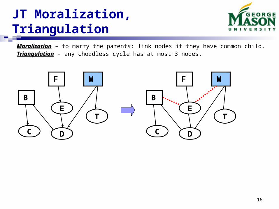
JT Moralization, Triangulation

MoralizationMoralization – to marry the parents: link nodes if they have common child.TriangulationTriangulation – any chordless cycle has at most 3 nodes.

T

F W

B

E

DC

T

F W

B

E

DC

17

JT Decomposition (for CLG only)

Any path between two discrete nodes that containing only continuous nodes is forbidden – we have to link these two discrete nodes to make the graph strongly decomposable.we have to link these two discrete nodes to make the graph strongly decomposable.

T

F W

B

E

DC

18

Clique and Junction Tree

Clique is a maximal and complete cluster of nodes (subset of variables) – if node S has link to all of nodes in clique U, node S belongs to clique U.

Clique tree is not unique.

T

F W

B

E

DC

BFE WFE

BED

WED

BC WT

19

Local Message Passing in JT

Next time.

20

Current Research about Direct Message Passing Algotithm

21

Pearl’s Message Passing Algorithm

In polytree, any node d-separate the sub-network above it from the sub-network below it. For a typical node X in a polytree, evidence can be divided into two exclusive sets, and processed separately:

Define messages and messages as:

Multiply-connected network may not be partitioned into two separate sub-networks by a node.

Then the belief of node X is:

22

Pearl’s Message Passing in BNs

In message passing algorithm, each node maintains Lambda message and Pi message for itself. Also it sends Lambda message to every parent it has and Pi message to its children.

After finite-number iterations of message passing, every node obtains its correct belief.

For polytree, MP returns exact For polytree, MP returns exact belief; belief; For networks with loop, MP is For networks with loop, MP is called loopy propagation that often called loopy propagation that often gives good approximation to gives good approximation to posterior distributions.posterior distributions.

23

Unscented Hybrid Loopy Propagation

UD

X

Weighted sum of continuous message.Weighted sum of continuous message.where is the function specified in CPD of X.where is the function specified in CPD of X.

Non-negative constant. Non-negative constant.

Weighted sum of continuous message.Weighted sum of continuous message.where is the inverse function. where is the inverse function.

Complexity is reduced significantly! Only depends on the size of discrete parents in local CPD.Complexity is reduced significantly! Only depends on the size of discrete parents in local CPD.

24

A

B

C

U

X

Y

W

Z