Orthogonal Functions: The Legendre, Laguerre, and Hermite Polynomials
26
General Orthogonality Legendre Polynomials Sturm-Liouville Conclusion Orthogonal Functions: The Legendre, Laguerre, and Hermite Polynomials Thomas Coverson 1 Savarnik Dixit 3 Alysha Harbour 2 Tyler Otto 3 1 Department of Mathematics Morehouse College 2 Department of Mathematics University of Texas at Austin 3 Department of Mathematics Louisiana State University SMILE REU Summer 2010 Coverson, Dixit, Harbour, Otto Orth.Funct. Leg., Lag. Hermite.
Transcript of Orthogonal Functions: The Legendre, Laguerre, and Hermite Polynomials
General OrthogonalityLegendre Polynomials
Sturm-LiouvilleConclusion
Orthogonal Functions: The Legendre,Laguerre, and Hermite Polynomials
Thomas Coverson1 Savarnik Dixit3 Alysha Harbour2
Tyler Otto3
1Department of MathematicsMorehouse College
2Department of MathematicsUniversity of Texas at Austin
3Department of MathematicsLouisiana State University
SMILE REU Summer 2010Coverson, Dixit, Harbour, Otto Orth.Funct. Leg., Lag. Hermite.

General OrthogonalityLegendre Polynomials
Sturm-LiouvilleConclusion
Outline
1 General Orthogonality
2 Legendre Polynomials
3 Sturm-Liouville
4 Conclusion
Coverson, Dixit, Harbour, Otto Orth.Funct. Leg., Lag. Hermite.

General OrthogonalityLegendre Polynomials
Sturm-LiouvilleConclusion
Overview
When discussed in R2, vectors are said to be orthogonal whenthe dot product is equal to 0.
w · v = w1v1 + w2v2 = 0.
Coverson, Dixit, Harbour, Otto Orth.Funct. Leg., Lag. Hermite.

General OrthogonalityLegendre Polynomials
Sturm-LiouvilleConclusion
Overview
Definition
We define an inner product (y1|y2) =∫ b
a y1(x)y2(x)dx wherey1, y2 ∈ C2[a,b].
DefinitionTwo functions are said to be orthogonal if (y1|y2) = 0.
DefinitionA linear operator L is self-adjoint if (Ly1|y2) = (y1|Ly2) for ally1,y2.
Coverson, Dixit, Harbour, Otto Orth.Funct. Leg., Lag. Hermite.

General OrthogonalityLegendre Polynomials
Sturm-LiouvilleConclusion
Trigonometric Functions and Fourier SeriesOrthogonality of the Sine and Cosine FunctionsExpansion of the Fourier Series
f (x) =a0
2+∞∑
k=1
(ak cos kx + bk sin kx)
Coverson, Dixit, Harbour, Otto Orth.Funct. Leg., Lag. Hermite.

General OrthogonalityLegendre Polynomials
Sturm-LiouvilleConclusion
Legendre Polynomials
Legendre Polynomials are usually derived from differentialequations of the following form:
(1− x2)y ′′ − 2xy ′ + n(n + 1)y = 0
We solve this equation using the standard power seriesmethod.
Coverson, Dixit, Harbour, Otto Orth.Funct. Leg., Lag. Hermite.

General OrthogonalityLegendre Polynomials
Sturm-LiouvilleConclusion
Legendre Polynomials
Suppose y is analytic. Then we have
y(x) =∞∑
k=0
akxk
y ′(x) =∞∑
k=0
ak+1(k + 1)xk
y ′′(x) =∞∑
k=0
ak+2(k + 1)(k + 2)xk
Coverson, Dixit, Harbour, Otto Orth.Funct. Leg., Lag. Hermite.

General OrthogonalityLegendre Polynomials
Sturm-LiouvilleConclusion
Recursion Formula
After implementing the power series method, the followingrecursion relation is obtained.
ak+2(k + 2)(k + 1)− ak (k)(k − 1)− 2ak (k)− n(n + 1)ak = 0
ak+2 =ak [k(k + 1)− n(n + 1)]
(k + 2)(k + 1)
Using this equation, we get the coefficients for the Legendrepolynomial solutions.
Coverson, Dixit, Harbour, Otto Orth.Funct. Leg., Lag. Hermite.

General OrthogonalityLegendre Polynomials
Sturm-LiouvilleConclusion
Legendre Polynomials
L0(x) = 1
L1(x) = x
L2(x) =12(3x2 − 1)
L3(x) =12(5x3 − 3x)
L4(x) =18(35x4 − 30x2 + 3)
L5(x) =18(63x5 − 70x3 + 15x)
Coverson, Dixit, Harbour, Otto Orth.Funct. Leg., Lag. Hermite.

General OrthogonalityLegendre Polynomials
Sturm-LiouvilleConclusion
Legendre Graph
Figure: Legendre Graph
Coverson, Dixit, Harbour, Otto Orth.Funct. Leg., Lag. Hermite.

General OrthogonalityLegendre Polynomials
Sturm-LiouvilleConclusion
Sturm-Liouville
A Sturm-Liouville equation is a second-order linear differentialequation of the form
(p(x)y ′)′ + q(x)y + λr(x)y = 0
p(x)y ′′ + p′(x)y ′ + q(x)y + λr(x)y = 0
which allows us to find solutions that form an orthogonalsystem.
Coverson, Dixit, Harbour, Otto Orth.Funct. Leg., Lag. Hermite.

General OrthogonalityLegendre Polynomials
Sturm-LiouvilleConclusion
Sturm-Liouville cont.
We can define a linear operator by
Ly = (p(x)y ′)′ + q(x)y
which gives the equation
Ly + λr(x)y = 0.
Coverson, Dixit, Harbour, Otto Orth.Funct. Leg., Lag. Hermite.

General OrthogonalityLegendre Polynomials
Sturm-LiouvilleConclusion
Self-adjointness
To obtain orthogonality, we want L to be self-adjoint.
(Ly1|y2) = (y1|Ly2)
which implies0 = (Ly1|y2)− (y1|Ly2)
= ((py ′1)′ + qy1|y2)− (y1|(py ′2)
′ + qy2)
=
∫ b
a(p′y ′1y2 + py ′′1 y2 + qy1y2 − y1p′y ′2 − y1py ′′2 − y1q1y2)dx
Coverson, Dixit, Harbour, Otto Orth.Funct. Leg., Lag. Hermite.

General OrthogonalityLegendre Polynomials
Sturm-LiouvilleConclusion
Self-adjointness
=
∫ b
a(p′y ′1y2 + py ′′1 y2 − y1p′y ′2 − y1py ′′2 )dx
=
∫ b
a[p(y ′1y2 − y ′2y1)]
′dx
= p(b)(y ′1(b)y2(b)−y ′2(b)y1(b))−p(a)(y1(a)y2(a)−y ′2(a)y1(a))
Coverson, Dixit, Harbour, Otto Orth.Funct. Leg., Lag. Hermite.

General OrthogonalityLegendre Polynomials
Sturm-LiouvilleConclusion
Orthogonality Theorem
TheoremIf (y1, λ1) and (y2, λ2) are eigenpairs and λ1 6= λ2 then(y1|y2)r = 0.
Proof.
(Ly1|y2) = (y1|Ly2)
(−λ1ry1|y2) = (y1| − λ2ry2)
λ1
∫ b
ay1y2rdx = λ2
∫ b
ay1y2rdx
λ1(y1|y2)r = λ2(y1|y2)r
(y1|y2)r = 0
Coverson, Dixit, Harbour, Otto Orth.Funct. Leg., Lag. Hermite.

General OrthogonalityLegendre Polynomials
Sturm-LiouvilleConclusion
Legendre Polynomials - Orthogonality
Recall the Legendre differential equation
(1− x2)y ′′ − 2xy ′ + n(n + 1)y = 0.
SoLy = ((1− x2)y ′)′
λ = n(n + 1)
r(x) = 1.
We want L to be self-adjoint, so we must determine necessaryboundary conditions.
Coverson, Dixit, Harbour, Otto Orth.Funct. Leg., Lag. Hermite.

General OrthogonalityLegendre Polynomials
Sturm-LiouvilleConclusion
Sturm-Liouville Problem - Legendre
For any two functions f ,g ∈ C[−1,1], by the general theory, weget ∫ 1
−1Lf (x)g(x)− f (x)Lg(x)dx
=
∫ 1
−1((1− x2)f ′)′g(x)− f (x)((1− x2)g′)′dx
= [(1− x2)(f ′g − g′f )]1−1= 0.
Coverson, Dixit, Harbour, Otto Orth.Funct. Leg., Lag. Hermite.

General OrthogonalityLegendre Polynomials
Sturm-LiouvilleConclusion
Legendre Polynomials - Orthogonality
Because (1− x2) = 0 when x = −1,1 we know that L isself-adjoint on C[−1,1].Hence we know that the Legendrepolynomials are orthogonal by the orthogonality theorem statedearlier.
Coverson, Dixit, Harbour, Otto Orth.Funct. Leg., Lag. Hermite.

General OrthogonalityLegendre Polynomials
Sturm-LiouvilleConclusion
Hermite Polynomials
For a Hermite Polynomial, we begin with the differentialequation
y ′′ − 2xy ′ + 2ny = 0
Coverson, Dixit, Harbour, Otto Orth.Funct. Leg., Lag. Hermite.

General OrthogonalityLegendre Polynomials
Sturm-LiouvilleConclusion
Hermite Orthogonality
First, we need to arrange the differential equation so it can bewritten in the form
(p(x)y ′)′ + (q(x) + λr(x))y = 0.
We must find some r(x) by which we will multiply the equation.For the Hermite differential equation, we use r(x) = e−x2
to get
(e−x2y ′)′ + 2ne−x2
y = 0
=⇒ e−x2y ′′ − 2xe−x2
y ′ + 2ne−x2y = 0
Coverson, Dixit, Harbour, Otto Orth.Funct. Leg., Lag. Hermite.

General OrthogonalityLegendre Polynomials
Sturm-LiouvilleConclusion
Hermite Orthogonality
Sturm-Liouville problems can be written in the form
Ly + λr(x)y = 0.
In our case, Ly = (e−x2y ′)′ and λr(x) = 2ne−x2
y .
0 = (Lf |g)− (f |Lg) =∫ ∞−∞
Lf (x)g(x)− f (x)Lg(x)dx
Coverson, Dixit, Harbour, Otto Orth.Funct. Leg., Lag. Hermite.
General OrthogonalityLegendre Polynomials
Sturm-LiouvilleConclusion
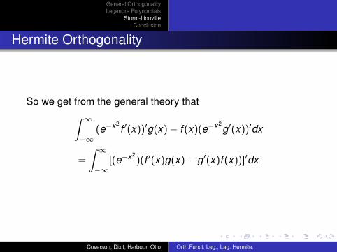
Hermite Orthogonality
So we get from the general theory that∫ ∞−∞
(e−x2f ′(x))′g(x)− f (x)(e−x2
g′(x))′dx
=
∫ ∞−∞
[(e−x2)(f ′(x)g(x)− g′(x)f (x))]′dx
Coverson, Dixit, Harbour, Otto Orth.Funct. Leg., Lag. Hermite.
General OrthogonalityLegendre Polynomials
Sturm-LiouvilleConclusion
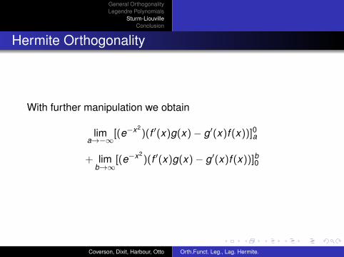
Hermite Orthogonality
With further manipulation we obtain
lima→−∞
[(e−x2)(f ′(x)g(x)− g′(x)f (x))]0a
+ limb→∞
[(e−x2)(f ′(x)g(x)− g′(x)f (x))]b0
Coverson, Dixit, Harbour, Otto Orth.Funct. Leg., Lag. Hermite.

General OrthogonalityLegendre Polynomials
Sturm-LiouvilleConclusion
Hermite Orthogonality
We wantlim
x→±∞e−x2
f (x)g′(x) = 0
for all f ,g ∈ BC2(−∞,∞). So we impose the followingconditions on the space of functions we consider
limx→±∞
e−x2/2h(x) = 0
andlim
x→±∞e−x2/2h′(x) = 0
for all h ∈ C2(−∞,∞).
Coverson, Dixit, Harbour, Otto Orth.Funct. Leg., Lag. Hermite.

General OrthogonalityLegendre Polynomials
Sturm-LiouvilleConclusion
Conclusion
Let φ1(x),φ2(x),...,φn(x),... be an system of orthogonal,real functions on the interval [a,b].Let f (x) be a function defined on the interval [a,b].
Assume that∫ b
a φ2n(x) 6= 0.
Suppose that f (x) can be represented as a series of theabove orthogonal system. That isf (x) = c0φ0(x) + c1φ1(x) + c2φ2(x) + · · ·+ cnφn(x) + · · ·
Coverson, Dixit, Harbour, Otto Orth.Funct. Leg., Lag. Hermite.

General OrthogonalityLegendre Polynomials
Sturm-LiouvilleConclusion
Conclusion
Multiplying f (x) by φn(x) to getf (x)φn(x) = c0φ0(x)φn(x) + c1φ1(x)φn(x) +c2φ2(x)φn(x) + · · ·+ cnφ
2n(x) + cn+1φn+1(x)φn+1(x) + · · ·∫ b
a f (x)φn(x)dx = cn∫ b
a φ2n(x)dx
Therefore cn =∫ b
a f (x)φn(x)dx∫ ba φ
2n(x)dx
are called the Fourier
coefficients of f (x) with respect to the orthogonal system.The corresponding Fourier series is called the Fourierseries of f(x) with respect to the orthogonal system.We may test whether this series converges or diverges.
Coverson, Dixit, Harbour, Otto Orth.Funct. Leg., Lag. Hermite.


![dvances - dmkrp.files.wordpress.com€¦ · 408 Dmitrii Karp -1 Here Wk, IL; and P~" is the k-th orthonormal polynomial of Hermite, Laguerre and Jacobi, respectively [19]. For the](https://static.fdocuments.net/doc/165x107/5f7ee79a8b3fb932d6131812/dvances-dmkrpfiles-408-dmitrii-karp-1-here-wk-il-and-p-is-the-k-th.jpg)