Originally published as -...

Originally published as: Nilsson, A., Holme, R., Korte, M., Suttie, N., Hill, M. (2014): Reconstructing Holocene geomagnetic field variation: new methods, models and implications. - Geophysical Journal International, 198, 1, p. 229-248 DOI: http://doi.org/10.1093/gji/ggu120

Geophysical Journal InternationalGeophys. J. Int. (2014) 198, 229–248 doi: 10.1093/gji/ggu120Advance Access publication 2014 May 15GJI Geomagnetism, rock magnetism and palaeomagnetism

Reconstructing Holocene geomagnetic field variation: new methods,models and implications

Andreas Nilsson,1 Richard Holme,1 Monika Korte,2 Neil Suttie1 and Mimi Hill11Geomagnetism Laboratory, Department of Earth, Ocean and Ecological Sciences, University of Liverpool, Oliver Lodge Laboratories,Oxford Street, Liverpool L69 7ZE, UK. E-mail: [email protected] Potsdam, Deutsches GeoForschungsZentrum-GFZ, Stiftung des off. Rechts Land Brandenburg, Telegrafenberg,D-14473 Potsdam, Germany

Accepted 2014 March 27. Received 2014 March 24; in original form 2013 November 21

S U M M A R YReconstructions of the Holocene geomagnetic field and how it varies on millennial timescalesare important for understanding processes in the core but may also be used to study long-termsolar-terrestrial relationships and as relative dating tools for geological and archaeologicalarchives. Here, we present a new family of spherical harmonic geomagnetic field modelsspanning the past 9000 yr based on magnetic field directions and intensity stored in archae-ological artefacts, igneous rocks and sediment records. A new modelling strategy introducesalternative data treatments with a focus on extracting more information from sedimentarydata. To reduce the influence of a few individual records all sedimentary data are resampledin 50-yr bins, which also means that more weight is given to archaeomagnetic data duringthe inversion. The sedimentary declination data are treated as relative values and adjustediteratively based on prior information. Finally, an alternative way of treating the sediment datachronologies has enabled us to both assess the likely range of age uncertainties, often up toand possibly exceeding 500 yr and adjust the timescale of each record based on comparisonswith predictions from a preliminary model. As a result of the data adjustments, power has beenshifted from quadrupole and octupole to higher degrees compared with previous Holocenegeomagnetic field models. We find evidence for dominantly westward drift of northern highlatitude high intensity flux patches at the core mantle boundary for the last 4000 yr. The newmodels also show intermittent occurrence of reversed flux at the edge of or inside the innercore tangent cylinder, possibly originating from the equator.

Key words: Archaeomagnetism; Palaeointensity; Palaeomagnetic secular variation.

1 I N T RO D U C T I O N

Global time-varying field models based on direct field measure-ments spanning the last few centuries (Bloxham et al. 1989; Blox-ham & Jackson, 1992; Jackson et al. 2000) have greatly improvedour understanding of the geomagnetic field and how it varies ondecadal to centennial timescales, but do not provide a record of suf-ficient length to understand the physical processes that control thelong-term changes in the geodynamo. Such models can be extendedto millennial timescales using global compilations of palaeomag-netic field measurements obtained from archaeological artefacts,igneous rocks and lake or marine sediments (Korte et al. 2005;Genevey et al. 2008; Donadini et al. 2009). Over recent years majorefforts have been made using these data compilations to reconstructnot only the dipole (Genevey et al. 2008; Knudsen et al. 2008; Valetet al. 2008; Nilsson et al. 2010) but also higher order structuresof the field (Hongre et al. 1998; Constable et al. 2000; Korte &Constable 2003; Korte et al. 2011; Licht et al. 2013).

Such reconstructions can be used in a wide range of applica-tions including investigations of westward and eastward motions inthe core (Dumberry & Bloxham 2006; Dumberry & Finlay 2007;Wardinski & Korte 2008), the dynamics of high latitude flux patches(Korte & Holme 2010; Amit et al. 2011), field asymmetry relatedto archaeomagnetic jerks (Gallet et al. 2009) and lopsided innercore growth (Olson & Deguen 2012), geomagnetic field shieldingof cosmic rays with implications for solar activity reconstructions(Muscheler et al. 2007; Snowball & Muscheler 2007; Lifton et al.2008) and as relative dating tools for geological and archaeologi-cal archives (Lodge & Holme 2009; Pavon-Carrasco et al. 2009;Barletta et al. 2010).

Palaeomagnetic data are usually divided into two groups: (i) ar-chaeomagnetic data (here taken to include lavas) containing spotreadings in time of both direction and intensity and (ii) sedimen-tary records constituting continuous depositional sequences of di-rections and relative intensities. Data from the latter group aregenerally considered less reliable but provide a better spatial and

C© The Authors 2014. Published by Oxford University Press on behalf of The Royal Astronomical Society. 229

at Bibliothek des W

issenschaftsparks Albert E

instein on October 21, 2014

http://gji.oxfordjournals.org/D

ownloaded from

mailto:[email protected]

http://gji.oxfordjournals.org/

230 A. Nilsson et al.

temporal (ST) geographical distribution, which is essential forglobal field modelling. Comparisons between dipole moment anddipole tilt reconstructions with more comprehensive spherical har-monic models highlight potential problems with recovering eventhe most basic (i.e. dipole) component of the field (Knudsen et al.2008; Valet et al. 2008; Nilsson et al. 2010). One of the mainreasons for these differences stems from the use and treatment ofsedimentary data to constrain the models. Several studies have notedinconsistencies within the current sedimentary database (Dona-dini et al. 2009), which are mainly due to dating uncertainties(Korte et al. 2009; Nilsson et al. 2010; Korte & Constable 2011;Licht et al. 2013), sometimes on the order of thousands of years(Doner 2003; Nourgaliev et al. 2005). In addition to uncertaintiesrelated to dating, the magnetic signal may also be both offset intime and inherently smoothed because of the gradual, but largelyunknown, process by which the magnetization is locked in to thesediments (see Roberts & Winklhofer 2004). Sedimentary recordscan also contain systematic errors in both declination and inclina-tion due to problems with orienting the retrieved sediment cores(e.g. Constable & McElhinny 1985; Ali et al. 1999; Snowball &Sandgren 2004; Stoner et al. 2007) but also due to different prob-lems related to sedimentary processes, such as compaction, whichmay lead to shallow inclinations (Blow & Hamilton 1978; Anson& Kodama 1987; Tauxe, 2005). A lack of consistent data treatmentand/or data availability makes it difficult to estimate these data un-certainties (Panovska et al. 2012).

In this study, we present three new palaeomagnetic field modelsspanning the last 9000 yr (pfm9k), building on the recent work ofKorte et al. (2011). One of the main purposes of this study is toaddress the issues with the sedimentary records mentioned above inorder to extract more information from this data set. We do this byintroducing new data treatments including redistributions of weightgiven to the different data sources and types during the inversion andnew adjustments/calibrations of relative data based on preliminaryfield estimates. The results are evaluated by comparisons with othermodels for the same time period and models based on synthetic datasets derived from the historical field model gufm1 (Jackson et al.2000).

2 DATA

2.1 Initial data set

The palaeomagnetic data used to develop the new models werebased on a similar initial data set used to construct CALS10k.1b(Korte et al. 2011). This data set consists of archaeomagnetic dec-lination, inclination and intensity data obtained from the onlineGEOMAGIA50 database (Donadini et al. 2006; Korhonen et al.2008) 2013 August 22, and sedimentary palaeomagnetic decli-nation, inclination and relative palaeointensity records from theSED12k data compilation (Donadini et al. 2009; Korte et al. 2011).

Prior to making any adjustments, the following data, regardedas unsuitable for the modelling procedure, were rejected or re-placed based on information in the original publications or compar-isons with other data: (i) two lake sediment records, Vatndalsvatn(Thompson & Turner 1985) and Lakes Naroch and Svir (Nourgalievet al. 2005) that were dated using bulk sediment radiocarbon datesthat produce suspiciously old ages, were removed. It is a knownproblem that radiocarbon dating of bulk sediments can produce tooold ages due to the incorporation of ‘old’ carbon from the bedrockor soil ‘diluting’ the contemporary 14C in the sediments (see, e.g.Bjorck & Wohlfarth 2001). In the case of Vatndalsvatn, for exam-

ple, the offset between calibrated 14C age and true age producedby this effect has been estimated to c. 1200 yr using a combina-tion of lead isotopes, caesium and radiocarbon analyses (Doner2003). (ii) Likewise all archaeomagnetic data with large dating un-certainties (σ age > 500 yr) were also removed. (iii) Two relativepalaeointensity records (AAM, WPA—see Table 1 for full names)and one declination record (VIC) were removed based on incom-patible long-term trends over the Holocene. If included, most of thedata from these records would be removed as outliers anyway dur-ing the model rejection analyses (see Section 3.1). (iv) Finally, therelative palaeointensity data from four Scandinavian lake records(FUR, FRG, MOT and SAR), which had been standardized for con-struction of a Fennoscandian master curve FENNORPIS (Snowballet al. 2007), were replaced with the originally published data (IanSnowball, 2012, personal communication).

2.2 Resampling the sedimentary data

The SED12k data compilation consists of a mix of data from singlecore studies represented by individual measurements to smootheddata stacks based on multiple measurements from several parallelcores. In addition, the measurements are either performed on dis-crete samples, collected every 2–3 cm, or on 1–2 m long u-channelssamples. The latter usually results in more data points, often with a1-cm resolution, but each measurement represents an average over adepth range of 15–20 cm depending on the size of the sense-coil andthe shape of the pick-up function (Weeks et al. 1993). The hetero-geneous nature of the data set leads to an inappropriate weightingof the data during the modelling. For example, a u-channel recordfrom a single core (WPA), which consists of correlated measure-ments, is represented by more than six times as many data pointsthan another arguably more reliable record (BIW) from the sameregion, based on measurements from three parallel cores, whereonly the smoothed data are available. To avoid such problems webinned all sedimentary records in 50-yr bins giving equal weight toeach site at any given time. This approach reduces the number ofsedimentary data by more than 70 per cent (from 67 802 to 19 865),which effectively adds weight to archaeomagnetic data.

2.3 Prior dipole field model

To rescale/adjust the sedimentary palaeomagnetic data and to as-sign intensity uncertainties we use a prior dipole field model. Thismodel was constructed by combining a dipole tilt reconstruction,DEFNBKE (Nilsson et al. 2011), based on selected sedimentary data,with a dipole moment estimate based on cosmogenic radionuclides.Cosmogenic radionuclides (e.g. 10Be, 14C) are produced in the atmo-sphere by interactions with cosmic rays at a rate which is inverselyrelated to the strength of the geomagnetic field (Lal & Peters 1967).To estimate variations in the dipole moment we used 10Be flux datafrom the GRIP ice core (Muscheler et al. 2004; Vonmoos et al.2006), which were first low-pass filtered with a cut-off frequency of1/3000 yr−1 to remove solar activity induced production variations(Muscheler et al. 2005). The 10Be flux data were then convertedto dipole moment using the transfer function from Lal (1988) andnormalized by minimizing the resulting dipole field model misfitto all available archaeointensity data (ignoring data uncertainty es-timates) over the model time period. The dipole component fromgufm1 was added to extend the model to the present, resulting in agap between 1350 and 1590 AD that was bridged by linear interpo-lation. See Section 4.2 (Fig. 6) for comparisons between the priordipole field model and other geomagnetic field models.

at Bibliothek des W




ownloaded from


Reconstructing Holocene geomagnetic field 231

Table 1. Summary of the sediment records used in this study.

Abb. Location Sample Nbina α63

b sFb �DMOD

c �DARCc �TAVG

d �TMAXd Ref.e

type (◦) (µT) (◦) (◦) (yr) (yr)

AAM Alaskan margin, Arctic Sea U-channel 112 3.5 – 14.7 – 108 400 1AD1 Adriatic Sea, Italy U-channel 122 3.5 6.2 – – −113 450 2AD2 Adriatic Sea, Italy U-channel 79 3.5 6.5 – – 192 500 2ANN Lac d’Annecy, France Discrete 43 3.4 – 3.0 (0.1) −42 305 3ARA Lake Aral, Kazhakstan Smoothed 25 3.5 – 14.7 (16.2) −259 400 4ASL Lake Aslikul, Russia Smoothed 72 3.5 – 9.5 (11.1) 360 500 5BAI Lake Baikal, Siberia, Russia Smoothed 61 3.5 6.7 (−6.6) −2.7 283 500 6BAM Lake Barombi Mbo, Cameroun Smoothed 131 3.5 – −3.5 – −55 300 7BAR Lake Barrine, North Queensland, Australia Discrete 169 6.7 4.9 34.4 (46.5) 26 200 8,9BEA Beaufort sea, Arctic Ocean U-channel 84 3.5 8.9 −28.2 (−33.3) −4 300 10BEG Lake Begoritis, Greece Discrete 106 2.5 – −1.5 (0.7) 35 250 11BIR Birkat Ram, Israel Discrete 106 4.1 6.1 (−2.0) −0.9 −181 450 12,13BIW Lake Biwa, Japan Smoothed 185 3.5 – 8.1 (9.0) 33 400 14BI2 Lake Biwa, Japan Smoothed 108 3.5 6.3 8.8 (11.8) 37 500 15BLM Lake Bullenmerri, Western Victoria, Australia Smoothed 83 3.5 – −3.1 (3.1) 27 195 16BOU Lac du Bourget, France Discrete 35 3.2 – −1.9 (0.5) 90 150 3CAM Brazo Campanario, Argentina Smoothed 137 3.5 – 0.6 – −77 300 17CHU Chukchi Sea, Arctic Ocean U-channel 155 3.5 7.5 −3.8 – −34 250 10DES Dead Sea, Israel Discrete 133 3.7 – −1.4 (−1.4) −150 500 18EAC Lake Eacham, North Queensland, Australia Discrete 106 7.5 6.5 13.7 (9.1) −10 150 8,9EIF Eifel maars, Germany Smoothed 185 3.1 – −0.2 (2.4) 194 500 19ERH Erhai Lake, China Discrete 109 4.5 – (−6.2) −4.6 98 500 20ERL Erlongwan Lake, China Smoothed 81 3.5 – 17.5 (19.2) −15 335 21ESC Lake Escondido, Argentina Smoothed 106 3.5 6.0 −2.8 – 25 300 22,23FAN Lake Fangshan, China Smoothed 114 3.6 – (1.0) 4.4 −139 500 24FIN 2 Finnish Lakes, Finland Smoothed 190 2.5 – −0.4 (4.0) −74 400 25FIS Fish Lake, Oregon, USA Discrete 145 4.1 – −2.2 (−1.9) 119 500 26FRG Frangsjon, Sweden Discrete 161 3.8 7.9 −2.1 (3.2) −163 450 27,28FUR Furskogstjarnet, Sweden Discrete 174 4.1 8.0 2.0 (3.9) 207 500 28,29GAR Gardar Drift, North Atlantic U-channel 168 3.5 7.4 (−14.3) −19.9 159 500 30GEI Llyn Geirionydd, Wales, UK Smoothed 128 3.5 – 1.0 (2.8) 80 300 31GHI Cape Ghir, NW Afr. Margin Discrete 117 4.3 6.3 −0.8 (2.8) 361 500 32GNO Lake Gnotuk, Western Victoria, Australia Discrete 135 4.0 – −2.0 (1.5) −21 300 16GRE Greenland, North Atlantic U-channel 162 3.5 – 8.0 (6.5) 144 450 33HUR Lake Huron, Great Lakes, USA Discrete 178 4.5 – 5.7 (9.1) 82 500 34ICE Iceland, North Atlantic U-channel 174 3.5 – −1.1 (−13.6) 103 300 33JON Jonian Sea, Italy U-channel 58 3.5 – −4.5 (−1.2) 361 500 2KEI Lake Keilambete, Western Victoria, Australia Discrete 175 3.3 – −0.8 (1.1) 52 200 16KYL Kylen Lake, Minnesota, USA Discrete 60 4.2 – (15.6) 17.0 218 500 35LAM Lake Lama, Siberia, Russia Discrete 182 4.4 – −9.0 – −60 500 36LEB Lake LeBoeuf, USA Smoothed 88 3.5 6.8 (0.8) 2.8 122 300 37LOM Loch Lomond, Scotland, UK Smoothed 122 3.5 – (−0.8) −0.1 −109 300 38LOU Louis Lake, Wyoming, USA Discrete 27 5.0 – 6.4 (5.5) 36 260 39LSC Lake St. Croix, Minnesota, USA Discrete 152 4.0 6.9 −0.3 (−1.7) 141 500 35MAR Mara Lake, British Columbia, Canada Smoothed 106 3.5 – 0.5 (1.8) −171 500 40MEE Meerfelder Maar, Germany Discrete 187 5.9 – 1.5 (5.6) 379 500 41MEZ Lago di Mezzano, Italy Discrete 105 3.7 7.5 (1.6) 0.7 78 300 42MNT Lago Morenito, Argenitna Smoothed 176 3.5 – 5.1 – 37 300 17MOR Lac Morat, Switzerland Discrete 35 3.2 – (3.9) 4.5 97 180 3MOT Motterudstjarnet, Sweden Discrete 163 4.1 7.8 −1.8 (3.3) 48 390 28,29NAU Nautajarvi, Finland Discrete 185 4.1 8.1 −6.8 (−1.7) −39 400 28,43PAD Palmer Deep, Antarctic Peninsula U-channel 165 3.6 7.3 -4.3 – −7 300 44PEP Lake Pepin, USA U-channel 146 3.5 6.3 – – 49 250 45POH Pohjajarvi, Finland Discrete 66 3.8 9.5 (0.6) 9.2 −80 390 46POU Lake Pounui, North Island, New Zealand Smoothed 41 3.5 – 4.1 (−3.3) 12 180 47SAG Saguenay Fjord, Canada U-channel 140 3.5 – (1.1) 8.7 103 300 48SAN Hoya de San Nicolas, Mexico Smoothed 113 3.5 – 3.7 (1.2) 6 100 49SAR Sarsjon, Sweden Discrete 155 3.9 8.0 (−0.1) 2.0 −108 435 27,28SAV Savijarvi, Finland Discrete 122 4.5 – (−4.0) 1.6 −232 500 28,50SCL Lake Shuangchiling, China U-channel 166 3.8 – (26.4) 24.0 −24 500 51STL St. Lawrence Est., Canada U-channel 150 3.5 6.6 19.0 (26.8) −143 500 52SUP Lake Superior, Great Lakes, USA Smoothed 184 3.6 – 4.0 (8.3) −105 400 53TRE Laguna el Trebol, Argentina Smoothed 141 3.5 5.8 7.9 – 18 240 54,55TRI Lake Trikhonis, Greece Discrete 133 2.9 – −2.4 (1.4) 243 500 11

at Bibliothek des W




ownloaded from



Table 1 (Continued).

Abb. Location Sample Nbina α63

b sFb �DMOD

c �DARCc �TAVG

d �TMAXd Ref.e

type (◦) (µT) (◦) (◦) (yr) (yr)

TUR Lake Turkana, Kenia Discrete 51 4.1 – – – −131 400 56TY1 Tyrrhenian Sea, Italy U-channel 61 3.5 – −0.6 (−1.5) 119 500 2TY2 Tyrrhenian Sea, Italy U-channel 79 3.5 – −0.5 (0.5) 190 450 2VIC Lake Victoria, Uganda Smoothed 143 3.5 – – – −10 150 57VOL Lake Volvi, Greece Discrete 50 2.9 – −1.9 (1.5) 265 500 11VUK Vukonjarvi, Finland Discrete 102 4.1 – −25.2 (−15.5) 225 500 58WA1 PS69/274–1, West Amundsen Sea Discrete 16 – 9.3 – – 41 385 59WA2 PS69/275–1, West Amundsen Sea Discrete 18 – 9.1 – – 316 500 59WA3 VC424, West Amundsen Sea Discrete 27 – 8.8 – – 104 400 59WAI Lake Waiau, Hawaii, USA Smoothed 109 3.5 – −3.1 (−3.4) −45 385 60WIN Lake Windermere, Northern England, UK Smoothed 137 3.5 – −3.9 (−2.5) 296 500 31WPA West Pacific, West Pacific U-channel 187 3.5 – – – 185 450 61aNumber of bins after resampling.bMean α63 and sF of binned data used for modeling.cDeclination adjustment (�D) based on prior dipole field model (MOD) or archaeomagnetic data (ARC). Adjustments not used are shown in brackets.dAverage and maximum timescale adjustments (�T), see Section 3.2.e1, Lise-Pronovost et al. (2009); 2, Vigliotti (2006); 3, Hogg (1978); 4, Nourgaliev et al. (2003); 5, Nurgaliev et al. (1996); 6, Peck et al. (1996); 7, Thouveny &Williamson (1988); 8, Constable & McElhinny (1985); 9, Constable (1985); 10, Barletta et al. (2008); 11, Creer et al. (1981); 12, Frank et al. (2002b);13, Frank et al. (2003); 14, Ali et al. (1999); 15, Hayashida et al. (2007); 16, Barton & McElhinny (1981); 17, Creer et al. (1983), 18, Frank et al. (2007);19, Stockhausen (1998); 20, Hyodo et al. (1999); 21, Frank (2007); 22, Gogorza et al. (2002); 23, Gogorza et al. (2004); 25, Haltia-Hovi et al. (2010); 26,Verosub et al. (1986); 27, Snowball & Sandgren (2002); 28, Snowball et al. (2007); 29, Zillen (2003); 30, Channell et al. (1997); 31, Turner & Thompson(1981); 32, Bleil & Dillon (2008); 33, Stoner et al. (2007); 34, Mothersill (1981); 35, Lund & Banerjee (1985); 36, Frank et al. (2002a); 37, King (1983);38, Turner & Thompson (1979); 39, Geiss et al. (2007); 40, Turner (1987); 41, Brown (1981); 42, U. Frank pres. comm.; 43, Ojala & Saarinen (2002);44, Brachfeld et al. (2000); 45, Brachfeld & Banerjee (2000); 46, Saarinen (1998); 47, Turner & Lillis (1994); 48, St-Onge et al. (2004); 49, Cha-parro et al. (2008); 50, Ojala & Tiljander (2003); 51, Yang et al. (2009); 52, St-Onge et al. (2003); 53, Mothersill (1979); 54, Gogorza et al. (2006);55, Irurzun et al. (2006); 56, Barton & Torgersen (1988); 57, Mothersill (1996); 58, Huttunen & Stober (1980); 59, Hillenbrand et al. (2010); 60, Peng & King(1992); 61, Richter et al. (2006.)

2.4 Calibration of sedimentary declination data

Sediment cores are usually azimuthally unoriented and palaeomag-netic declination data measured on sediments are therefore mostlypublished as relative values, calculated by removing the averageover the whole sequence. While in many cases this approach willlead to reasonable results, there is a risk of introducing systematicerrors to the data. The cores could potentially be oriented by fittingthe declination data from the top of the sequence to historical fieldmeasurements (Constable et al. 2000), or alternatively to palaeo-magnetic measurements of nearby lava flows correlated in timevia tephra layers associated with the same eruption (Verosub et al.1986). However, the sediments from the top of the core or next totephra layers are often not ideal recorders of the geomagnetic fieldand therefore such adjustments could be problematic. Another prob-lem is that the data published as relative declination are frequentlyprovided to the database as absolute values (i.e. before removingthe long-term average) and may therefore be mistaken for orienteddata. To reduce any systematic errors introduced to the databaseby such type of core reorientations, or lack of reorientations, weadjust each sedimentary declination record by a constant number ofdegrees based on comparisons with the prior dipole field model or,when appropriate, archaeomagnetic data.

For each record, a first correction was determined as the mediandifference between the prior dipole model prediction and the data.Archaeomagnetic data were then selected from within a radius of3000 km from each site and relocated using virtual geomagneticpoles (VGPs). Both the sedimentary and the archaeomagnetic dec-lination data were smoothed with a 200-yr moving window at 100-yrintervals and if there were enough overlapping data points (at least10), a second correction was determined as the median differencebetween the smoothed data. The smoothing of the data produces

more stable adjustments by restricting the comparison to the morerobust long-term variations. To avoid corrections based on spuriousdata the second correction constant was used only in cases whenthe archaeomagnetic data provided a better fit to the data than thedipole field model, calculated as the mean of the absolute residu-als. The difference between the adjustments predicted by the priormodel and the archaeomagnetic data in regions where both couldbe determined is on average around 3.4◦ (Fig. 1). A summary of alladjustments can be found in Table 1.

The choice of a suitable radius for the selection of archaeomag-netic data is a trade-off between obtaining enough data used tocalculate the adjustment while limiting the selection to an area withsimilar geomagnetic field history. A 3000 km radius can be consid-ered quite large, however; given the Earth’s ∼40 000 km circumfer-ence, the corresponding 6000 km wavelength translates to sphericalharmonic degree 6–7, which is roughly the spatial resolution ofour final models (see Fig. 5). We found that the corrections calcu-lated based on a smaller radius often lead to regionally inconsistentadjustments, mainly because of an over-reliance on individual ar-chaeomagnetic data points. The declination adjustments based ona 3000 km radius produce a regionally consistent data set, whichdiffer slightly but systematically from the predictions of the priordipole field model (Fig. 1c).

2.5 Scaling of relative palaeointensity

The sedimentary relative palaeointensity data were converted toabsolute palaeointensites, following the approach of Korte &Constable (2006) and Donadini et al. (2009), by multiplying eachentire record with a constant scaling factor. As for the declinationdata, the scaling factor was calculated based on the prior dipole fieldmodel or using archaeomagnetic intensity data, where possible. The

at Bibliothek des W




ownloaded from



Figure 1. The mean difference between the declination predicted by eitherregional archaeomagnetic data (DARC) or the dipole prior (DMOD) and thedeclination from each sediment record (DSED) over overlapping time inter-vals. Upper panel (a and b) shows the mean difference determined for allrecords within each grid-cell and lower panel (c) shows the mean differencebetween adjustments determined using archaeomagnetic data and the dipoleprior within each grid, where applicable.

scaling factor was determined as the median ratio of the referencepalaeointensity data over the relative palaeointensity data.

For each record, a first scaling factor was determined based onthe prior dipole field model. The archaeomagnetic data were se-lected using the same criteria as for the declination adjustments andsmoothed using the same 200-yr moving window and used to cal-culate a second scaling factor. As for the declination corrections thesecond scaling factor was only used when the archaeomagnetic dataprovided a better fit to the data than the prior dipole field model,calculated as the mean of the absolute residuals. The scaling factorscalculated based on the prior dipole model did not differ consider-ably (on average 4.5 per cent) from those based on archaeomagneticdata.

Relative palaeointensity reconstructions can be sensitive tochanges in the depositional environment through time and suchchanges could lead to different scaling factors being appropriate fordifferent parts of the sequence. In two cases (LSC at 600 BC andTRE at 0 AD), we found sudden jumps in the data that we identifiedas such changes in the depositional environment. In both cases sus-

piciously large changes in the relative palaeointensity could also betraced back to similar changes in concentration dependent mineralmagnetic parameters at corresponding depths in the original studies(Lund & Banerjee 1985; Gogorza et al. 2006). To avoid applyinginappropriate scaling factors both records were split into two parts,which were rescaled separately and then joined back together. Wesuspect that other relative palaeointensity records may suffer fromsimilar problems, potentially with more gradual changes makingthem more difficult to identify. Improvements in both the identifica-tion and correction of this problem should be investigated in futurestudies.

2.6 Assigning error estimates

Uncertainty estimates of palaeomagnetic data are often poorly de-fined and sometimes not provided at all. Mostly this is because thereare too few measurements to allow a precise estimate of the disper-sion, but additionally unknown systematic errors also appear to beimportant, particularly for palaeointensity data (Suttie et al. 2011).As discussed by Korte et al. (2005) and Donadini et al. (2009) thepublished error estimates come from a wide array of different anal-yses and forms. The norm is to give uncertainty estimates in termsof the α95 confidence circle of the direction (Fisher 1953), and thestandard deviation (σ F) of the intensity measurements. The α95 isconveniently converted to a standard angular error (α63) using

α63 = 81

140α95. (1)

For the purposes of constructing a global field model it is impor-tant to use consistent uncertainty estimates to weight the individualdata. To address these problems Donadini et al. (2009) assigned aminimum α63 error of 2.5◦ (3.5◦) for archaeomagnetic (sedimen-tary) directional data and a minimum σ F of 5 µT for all inten-sity data. These estimates, which were also assigned to data withunknown error estimates, were based on the average deviation of thedata from the gufm1 historical model between 1590 and 1990 AD.Using smoothing spline fits devised to capture the robust variationof each record Panovska et al. (2012) concluded that the minimumerrors assigned to the sedimentary data by Donadini et al. (2009)are probably too small. In an effort to favour high-quality dataLicht et al. (2013) opted to keep the original error estimates, whenavailable, and instead introduced a modelling error of α63 = 2◦

for directions and σ F = 2 µT for intensity, which was added inquadrature to the data uncertainty. They argued that although high-quality data cannot be fitted too closely by the model this limitationis mainly related to the limited resolution of the model and not thedata uncertainty. To penalize data with unknown uncertainty Lichtet al. (2013) assigned a root mean square (rms) value of all availablepublished errors for each data type multiplied by a factor of 1.5.

In this study, we acknowledge that the published error estimatesmay fail to account for unknown systematic errors and have there-fore opted for an approach similar to that of Donadini et al. (2009)using a set of minimum error estimates. However, to penalize datawith less well-defined uncertainties, different minimum errors wereassigned depending on the number of samples/specimens (N/n) usedto calculate the mean direction or intensity.

Archaeomagnetic directions were assigned with a minimumα63 = 2.5◦ for N ≥ 5, α63 = 3.5◦ for N < 5 and α63 = 4.5◦ fordata with unknown uncertainties. Because most archaeomagneticdirections are determined using at least five samples, we chose toalso use a minimum α63 = 2.5◦ for data where N was unspeci-fied. For archaeomagnetic intensities we first converted the σ F tostandard errors of the mean (sF), which is more consistent with the

at Bibliothek des W




ownloaded from



treatment of the directional uncertainties, using

sF = σF√n

, (2)

where n is the number of specimens. Given enough data sF shouldprovide a good estimate of the experimental error. However, asnoted by Suttie et al. (2011) the published errors appear to accountonly for a small fraction of the actual error budget, which is im-plied by the usual choice of σ F as the uncertainty. Through directcomparisons with gufm1 Suttie et al. (2011) suggested an appropri-ate minimum error in the range of 10–15 per cent of the true fieldstrength. Expressing the error in terms of a percentage of the truefield, rather than a fixed value of for example 5 µT, would have theadvantage of not underweighting data from lower latitudes wherethe field is weaker, if uncertainties are proportional to field intensity.Based on these observations the intensity data were assigned withminimum sF = 10 per cent for n ≥ 5, sF = 12 per cent for n < 5 andsF = 14 per cent for unknown uncertainties. The true field strengthat a given location and time was approximated using predictions ofthe prior dipole field model.

The sedimentary directional data consist of discrete sample mea-surements (31 records), different forms of running averages (25records) and u-channel measurements (17 records). The data, espe-cially from the second group, are sometimes published with someform of uncertainty estimate. However, out of all these records only10 are provided with an error estimates in the database. These comein the form of α95 confidence limits (2), (angular) standard devia-tions (4) and maximum angular deviations (4). In order to treat thedata consistently only the first were deemed suitable for the mod-elling purposes. These α95 confidence limits are based on stacks of12 (EIF) and 8 (FIN) parallel cores with equivalent α63 rms val-ues of 3.05◦ and 1.88◦, respectively. While these errors may notbe representative of all sedimentary data, the latter study (Haltia-Hovi et al. 2010) in particular highlights the potential precisionwith which the directions can be acquired given enough data. Basedon the assumption that most hidden or systematic errors associatedwith sedimentary data are due to chronologic uncertainties, whichare dealt with separately in Section 3.2, and problems with coreorientation, partly solved by the declination adjustments, we treaterror estimates in a similar way to the archaeomagnetic errors.

For the purpose of error assignment the sedimentary data canbe divided into two groups: (i) records containing independentdata from discrete samples and (ii) smoothed records (includingu-channels) containing non-independent data. From the resamplingof the data we obtain uncertainty estimates for both directions andrescaled intensities based on the dispersion of the data within each50-yr bin. For data from the first group, with no prior error estimates,the resulting uncertainty estimates are treated in the same way asthe archaeomagnetic data using the same minimum α63 and sF as-signed based on the number of samples used to calculate the meanvalues. For the data from the second group information is missingregarding both the number of independent data points and the truedispersion of the data. The provided α95 estimates from EIF andFIN were converted to α63 and transferred to binned error estimatesthrough error propagation. Data from these two records were thenassigned a minimum α63 = 2.5◦ while the uncertainty estimates,calculated from the binned data, from the remaining records weretreated as less well defined and assigned a minimum α63 = 3.5◦.None of the rescaled intensity error estimates from the second groupprovided in the database were deemed suitable and therefore all un-certainty estimates, calculated from the binned data, were assigneda minimum sF = 12 per cent. The strategy used here to assign uncer-

tainties to sedimentary data results in larger errors on average forboth directions (3.8◦) and intensities (7.1 µT) compared to the min-imum values of 3.5◦ and 5 µT assigned by Donadini et al. (2009).However the methodology also allows for slightly smaller error esti-mates: 10 per cent of the α63 are smaller than 3.5◦ and 11.5 per centof the sF are lower than 5 µT. The average α63 and sF from eachrecord are listed in Table 1.

For the modelling procedure we want to treat inclination anddeclination separately. This is particularly important for the sed-imentary data where each component might be associated withindependent errors, such as core rotation affecting declination dataand sediment compaction affecting the inclinations. Consequentlyall α63 error estimates were converted to inclination errors (sI = α63)and to declinations errors (sD) using

sD = α63

cos I, (3)

where I is the inclination. Age uncertainties (σ A) for archaeomag-netic data, derived from GEOMAGIA50, were assigned a minimumvalue according to the age of the sample (σ A = 100 yr prior to 1000AD, σ A = 50 yr from 1000 to 1700 AD and σ A = 0 yr from1700 AD to present) to avoid overestimating the error of historicaldata. Archaeomagnetic data with unknown age uncertainties wereassigned with the same minimum σ A plus 50 yr. Sedimentary ageuncertainties are more difficult to quantify for individual samples asthey are usually derived from some form of interpolation betweena few dated levels in the sediment column. Additional unknownuncertainties such as ‘old’ carbon ‘diluting’ the contemporary 14Cin the sediments (Bjorck & Wohlfarth 2001), potential hiatuses inthe stratigraphy and lock-in delays of the remanent magnetization(Roberts & Winklhofer 2004) further complicate the age determi-nation. To deal with these problems we have introduced a new wayof treating the age uncertainties of sedimentary data in which allrecords are treated equally, see Section 3.2.

3 M O D E L L I N G M E T H O D

3.1 Initial model

The pfm9k models are constructed using an expansion on a sphericalharmonic basis in space and cubic B-splines in time. The method-ology follows that of Bloxham & Jackson (1992) used for historicalfield models and adapted for archaeomagnetic and palaeomagneticdata by Korte & Constable (2005, 2011) and Korte et al. (2009).We assume an electrically insulating mantle and neglect crustalfields and external (ionospheric and magnetospheric) fields. Thetime-dependent geomagnetic field, B(t), is described as the negativegradient of a scalar potential V(t) everywhere outside the Earth’score.

B(t) = −∇V (t). (4)

This potential can be expanded as a series of spherical harmonics

V (r, θ, φ, t) = almax∑l=1

l∑m=0

(a

r

)l+1[gm

l (t) cos(mφ) + hml (t) sin(mφ)

]

× Pml (cos θ ), (5)

where (r, θ , φ) are spherical polar coordinates (r is the radius fromEarth’s centre, θ is the colatitude and φ is the longitude), t is time,a = 6371.2 km (the mean radius of the Earth’s surface) and lmax

is the truncation point of the expansion in spherical harmonics.The Pm

l (cos θ ) are Schmidt quasi-normalized associated Legendre

at Bibliothek des W




ownloaded from



functions of degree l and order m. The structure of the field isdefined by the time-dependent Gauss coefficients {gm

l ; hml }, which

are expanded on a basis of N cubic B-splines, M,

gml (t) =

N∑n=1

gm,nl Mn(t) (6)

with a similar expansion for hml .

The spherical harmonic basis is expanded to degree 10 and theknot space is chosen as 50 yr. However, the actual ST resolution ofthe model will be lower and is determined by data and regularization.To find the smoothest, simplest model that satisfactorily fits thedata we minimize the misfit to the data and two model norms,one measuring the roughness in the spatial domain and one inthe temporal domain. For the spatial norm we use the physicallymotivated lower bound on Ohmic dissipation (Gubbins 1975) at thecore mantle boundary (CMB; r = c), given by

� = 4π

te − ts

te∫ts

f (Br )dt (7)

with

f (Br )=lmax∑l=1

(l+1)(2l+1)(2l+3)

l

(a

c

)2l+3 l∑m=0

[(gm

l

)2+(hm

l

)2].

(8)

For the temporal norm we use

= 1

(te − ts)

te∫ts

∮

CMB

(∂2t Br )2d�dt (9)

where [ts, te] is the time interval over which we solve the field.The coefficients from eq. (6) are represented by a model vec-

tor m = (g0,11 , g1,1

1 , h1,11 , . . . , g0,2

1 , . . .). The palaeomagnetic data,directions and intensity, are non-linearly related to the coefficientsand we therefore have to find a solution iteratively from linearizedequations. We use a constant axial dipole of g0

1 = 30 µT as a startingmodel, convergence is reached quickly and we always choose the5th iteration as the final model. The resulting objective function tobe minimized is

(γ − fm)TC−1e (γ − fm) + λs� + λT , (10)

where (γ − fm) is the residual vector given by the difference be-tween data γ and model m related through the operator f accordingto eq. (4) and Ce is the data error covariance matrix, with dampingparameters λS and λT. Based on the argument that a dipole field is abetter smooth field assumption than a zero field (Korte et al. 2009),we exclude the dipole terms from the spatial regularization.

The damping parameters for the preferred model were chosenby visual comparison (Lodge & Holme 2009) of the time-averagedgeomagnetic power spectra of the main field and secular variationto those of the historical field model gufm1 and the high resolu-tion palaeomagnetic field model CALS3k.4 (Korte & Constable2011), respectively. The chosen regularization norms result in rela-tively stronger damping of power in main field and secular variationfor higher spherical harmonic degrees (i.e. small-scale/short-termstructure) compared to lower spherical harmonic degrees. We as-sume that a reasonable solution does not show more spatial com-plexity on average than the historical field and λS is chosen usingthe average main field power spectra of gufm1 as a template. Weattempt to preserve, or avoid exceeding, the relative proportions ofthe power spectra by limiting the ‘allowed’ power in each spherical

harmonic degree based on the power of lower spherical harmonicdegrees, according to the gufm1 power spectrum. Given the largedating uncertainties associated with the palaeomagnetic data, wealso assume that a reasonable solution will not be able to capturevariations on timescales shorter than 300–400 yr. To produce a suit-able template for the secular variation power spectra based on thiscriterion we filter the CALS3k.4 Gauss coefficients with a 350-yrrunning average and λT is chosen by comparison to the average sec-ular variation power spectrum of this temporally smoothed versionof the CALS3k.4 model.

The models were built iteratively in several steps: (i) first a pre-liminary model A was constructed based on all data with the adjust-ments described above. (ii) A residual analysis was carried out anddata lying more than three standard deviations in data uncertaintyfrom the preliminary model predictions were rejected as outliers.Because the errors of the data are largely unknown we used themean rather than the individual data uncertainty to identify dataoutliers. The mean data uncertainty was calculated independentlyfor declination, inclination and intensity. To account for the greatervariability of declination data associated with steeper directions, thedeclination errors (and residuals) used in the residual analysis wereconverted back to α63 using the inverse of (3)

α63 = sD cos(Ip), (11)

where Ip is the inclination of the model prediction. Following a sim-ilar argument, all intensity errors (and residuals) were normalizedby the intensity predicted by the model. A new model B1 was con-structed based on the outlier free data. (iii) The sediment declinationdata and relative palaeointensity records, based on the outlier freedata set, were recalibrated using the B1 model and a third model C1constructed.

The last two steps were repeated. After the first iteration6.5 per cent of the declination data were rejected (cutoff = 11.15◦),6.4 per cent of the inclination data (cutoff = 10.62◦) and 5.1 per centof the intensity data (cutoff = 37.50 per cent). The absolute changein the declination and relative palaeointensity calibration factorsafter the first iteration were on average 1.9◦ and 2.9 per cent, re-spectively, with changes up to 8◦ (mainly high latitude sites) and10 per cent required for some records. After the third iteration lessthan 0.2 per cent of the data were rejected and changes to the cal-ibration factors were reduced to on average 0.2◦ and 0.3 per cent.The final model pfm9k.1 was chosen as model B3. To minimizeend effects associated with the B-spline functions the model is de-termined for the period between 7500 BC and 2000 AD but weonly show results from 7000 BC to 1900 AD. We decided to keepa relatively larger part of the recent end of the model in order to beable to validate the model against gufm1, even though this part ofthe model will include some spline end effects.

Regularized models will tend to underestimate, rather than over-estimate, the intensity with respect to the data. This is true even ifwe exclude the dipole coefficients from the regularization, as canbe seen in Table 2. The problem can be exacerbated by the inclu-sion of sedimentary relative palaeointensity records, particularlyif they are rescaled using a model that is already underestimatingthe intensity. Including iteratively rescaled sedimentary data in theresidual analysis may also produce near evenly distributed inten-sity residuals hiding the fact that the model is underestimating theabsolute intensity data. This is partly resolved by resampling thesedimentary data, effectively increasing the weight of the archaeo-magnetic, absolute, intensity data. To further improve the fit wealso increased the weight given to all intensity data by 50 per cent,which was achieved by reducing the uncertainty estimates of thedata accordingly during the inversion process. A similar approach

at Bibliothek des W




ownloaded from



Table 2. Model-data residuals, archaeomagnetic data.

Modela NARCb FAVG

c rmsFd rmsARC

d

ARCH3k.1 10110 1.09 1.46 1.57CALS10k.1b 12043 3.23 1.77 1.88Dipole field prior 12043 − 0.15 1.72 2.19pfm9k.0 (initial) 12043 2.97 1.78 1.81pfm9k.0 (dec. data adjusted) 12043 2.48 1.75 1.79pfm9k.0 (sed. data resampled) 12043 1.16 1.64 1.69pfm9k.1 (increase weight to F) 12043 0.66 1.58 1.69pfm9k.1a (sed. timescales adjusted) 12043 0.72 1.58 1.68aDifferent pfm9k models listed with more data treatments (in brackets)added successively from top to bottom.bNumber of archaeomagnetic data (dec + inc + F) between −7000 and1900 AD used for the residual analyses.cAverage intensity residuals (FDATA − FPRED).dThe rms of residuals for intensity and all data, normalized by their individ-ual uncertainty estimates.

was used by Korte & Constable (2005), but with a 100 per cent in-crease in the weight. We found that a 50 per cent increase provided agood balance between improving the model fit to the intensity data,reducing the model underestimation, while not markedly changingthe overall rms misfit to the data (including directions).

3.2 Addressing sediment age uncertainties

The age uncertainties of the data are often not well constrained andtherefore applying a strong temporal damping seems a reasonableapproach. This will be effective if the age uncertainties can be con-sidered to be non-systematic, for example for the archaeomagneticdata where most data points have been dated individually. However,for the sedimentary data the age estimates can be both systematicallywrong, for example due to reservoir effects affecting the radiocar-bon dates, and have correlated errors due to the interpolation ofages when constructing an age depth model. Given the stratigraphicinformation of the data we can attempt to correct for this by findingan optimal age-depth model for each sedimentary record based oncomparisons to a preliminary model prediction (Fig. 2). In regionswhere the model is not overly dependent on individual records thisapproach should be able to correct for inconsistencies in the dataset that are due to incompatible age-depth models. In contrast, inregions where data are scarce this approach will result in few or noadjustments to the timescales. For this analysis we used the initialdata set (before outlier rejection) and the pfm9k.1 model.

Based on an approach previously used by Nilsson et al. (2011)the individual timescales of the sedimentary records were randomlystretched and compressed, allowing for a maximum timescale ad-justment of Tlim = (±)500 yr for each data point while still pre-serving the stratigraphic relationship. In practice these adjustmentswere achieved by dividing each timescale, from −7000 to 2000AD, into 500-yr blocks. Using 2000 AD as a fixed starting pointand moving back in time, each block was then randomly stretched orcompressed by up to 30 per cent (using 50-yr steps) while keepingwithin the ±500 yr limits of the original age estimates. To explorethis rather large parameter space and to find the timescale adjustmentthat is most compatible with the model we use a nested samplingapproach (Skilling 2006). Briefly explained we start off with a setof 50 randomly adjusted timescales. Each timescale adjustment isranked by the χ 2 sum of the model-data residuals normalized bythe data uncertainties

χ 2 =∑

i

(Ds − Dpi)2

s2Di

+∑

j

(Ij − Ipj)2

s2Ij

+∑

k

(Fk − Fpk)2

s2Fk

, (12)

where D, I and F are the declination, inclination and intensity dataand Dp, Ip and Fp the equivalent model predictions. Iteratively theworst ranking timescale is replaced by a variation of one of the49 remaining timescales, if it results in an improved χ2. We foundthat 500 000 iterations was usually enough to isolate the best-fittimescale adjustment. After adjusting the timescales of all sedi-ment records a new model, pfm9k.1a, was produced using the sameapproach and the same damping parameters used for pfm9k.1.

Adjusting the timescale is justified if it leads to a significantlybetter fit; in particular if the ratio of likelihoods exceeds a certainthreshold. The log likelihood of the unadjusted data (L0) and theadjusted data (LA) can be expressed as

log L0 = c − χ 20

2(13)

and

log LA = c − χ 2A

2, (14)

where c is some constant. To see if adjustment A is justified wecalculate the odds. H is the hypothesis that the time should be leftunchanged. Bayes theorem says the probability of H and A givendata R, where P(H) is the prior probability of H and P(A) is the priorprobability of A, are given by

P(H |R) = L0 P(H )

P(R)(15)

and

P(A|R) = LA P(A)

P(R). (16)

We should prefer A over H if

P(A|R)

P(H |R)> 1 (17)

or if

log LA − log L0 > logP(H )

P(A). (18)

The ratio of prior probabilities is simply the size of the spacethat A was picked from (assuming a uniform prior for A). This isof the order 718 for the maximum of 18 different blocks, each onewhich can be moved in up to seven different ways with respect tothe adjacent block. Therefore, the time adjustment is justified if

χ 2A

2− χ 2

0

2> Nblocks log 7. (19)

We find that this condition is satisfied for about 90 per cent of therecords (the remaining 10 per cent are mostly represented by recordswhere the analysis resulted in only minor timescale adjustments) andtherefore conclude that the timescale adjustments can be consideredjustifiable.

In Fig. 2, we show examples from three different records ofdata plotted against their original timescales and the optimally ad-justed timescales compared with predictions of the pfm9k.1 model.All three records show time adjustments of 300 yr or more, bothtowards younger and older ages. The top 4000 yr from the FishLake record (FIS) has been shifted on average 288 yr towardsyounger ages. This is supported by a similar adjustment of ∼280yr which was suggested by Hagstrum & Champion (2002), due tocalcium carbonate dilution of the bulk 14C samples used to date therecord. The Fish Lake chronology was also forced to fit an indepen-dent age estimate of the Mazama Tephra layer, of about 4800 BC

at Bibliothek des W




ownloaded from



Figure 2. Example of timescale adjustments, shown for (a) Fish Lake, (b) Loch Lomond and (c) Lake Aslikul. For each example the subplots are organized asfollows: Inclination (upper left), declination (lower left) and timescale (right). Original timescale (blue), adjusted timescale (red) and pfm9k.1 model prediction(black). The light grey shaded area shows the minimum and maximum allowed timescale adjustments.

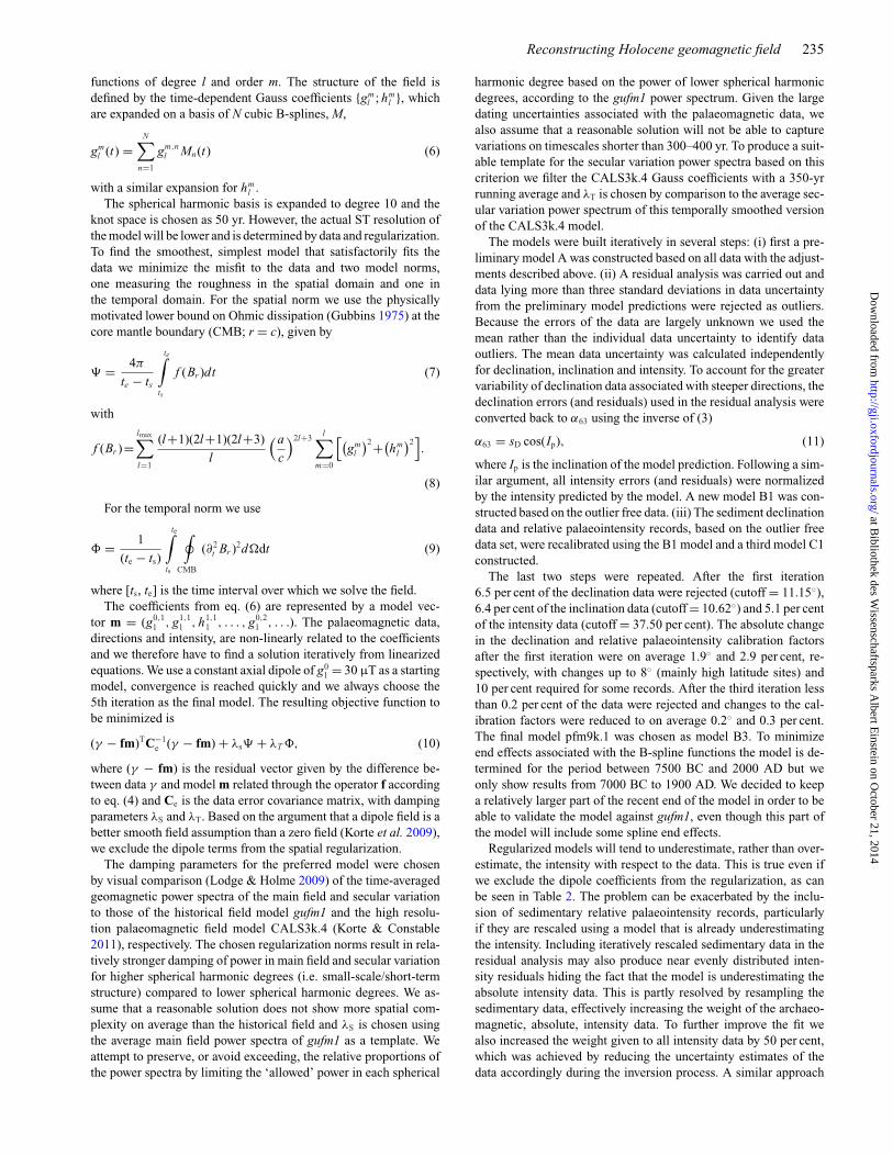
(Verosub et al. 1986), which explains why the model predictsonly minor time adjustments for this older part of the record.Fig. 3 shows the distribution of timescale adjustments defined as�T = Tadjusted − Toriginal, where T is the age estimate of individ-ual data points. Overall the distribution is slightly skewed towardsyounger ages, particularly for the last 3000 yr where the modelis more heavily constrained by archaeomagnetic data. This couldsuggest either a widespread ‘old’ carbon problem affecting the ra-diocarbon based chronologies or possibly a predominant lock-indelay effect.

3.3 Addressing all data uncertainties

To investigate the effects of magnetic and age (MA) uncertaintiesas well as the impact of the ST distribution of the data we used theMAST bootstrap methodology, described in detail in Korte et al.(2009). First a temporary model pfm9k.1B was constructed based

on the same approach as above but with a more relaxed tempo-ral damping, chosen by visual comparison to the secular variationpower spectra of gufm1. For each of the 2000 bootstrap samples wecreated data sets by drawing on the final pfm9k.1B data set. Thebootstrap models were constructed without further iterative recali-bration or rejection of data and using the same damping parametersas for pfm9k.1B. The simulated data at each location were gener-ated in two steps with slight differences for archaeomagnetic andsedimentary data. (i) In the first step the archaeomagnetic data wereindependently sampled from two normal distributions, one centredon the value of the magnetic component with a standard deviationcorresponding to the data uncertainty estimate, and the other cen-tred on the age estimate and using its respective standard error. Forthe sedimentary data the sampling of each datum from a normaldistribution centred on the magnetic component was done in thesame way. However, for the temporal sampling the timescale ofeach record was instead randomly stretched and compressed using

at Bibliothek des W




ownloaded from



Figure 3. Histogram of all timescale adjustments made to the sedimentarydata defined as �T = Tadjusted − Toriginal, where T is the age estimate ofindividual data points. Also shown are the distributions of �T for the last3000 yr (solid green line), between 4000 and 1000 BC (long dashed redline) and between 7000 and 4000 BC (short dashed blue line).

the same routine described above. This introduces rather large, butfrom what we can infer from the analysis in Section 3.2 also quiterealistic, chronological errors that increase with age. (ii) In the sec-ond step, bootstraps were performed on these data sets, where forthe archaeomagnetic data the number of data locations was keptconstant and values picked by uniform random sampling from thatdata set. For the sediments, the number of records was kept fixed andthe locations again uniformly sampled. The final model, pfm9k.1b,was based on the average of the 2000 bootstrap models and theuncertainties determined as standard deviation of the coefficients.The number of 2000 models was found to be enough to reach con-vergence.

4 M O D E L R E S U LT S A N DC O M PA R I S O N S

We have constructed three new models of the geomagnetic fieldvariation for the last 9000 yr; (i) pfm9k.1 based on the initial dataset with strong temporal damping, (ii) pfm9k.1a based on an opti-mally timescale-adjusted data set with strong temporal damping and(iii) pfm9k.1b: the average of 2000 bootstrap models with weaktemporal damping.

4.1 Model-data comparisons

By reducing inconsistencies in the sedimentary age estimates,pfm9k.1a is able to capture larger amplitude palaeosecular vari-ation (PSV) than other models that include sedimentary data, suchas pfm9k.1b and CALS10k.1b (Fig. 4). The predictions of pfm9k.1aare in good agreement with models based on archaeomagnetic data,for example A_FM (Licht et al. 2013) and ARCH3k.1 (Korte et al.2009), for the northern hemisphere sites where the latter modelscan be considered more robust. Well known PSV features suchas the westward declination swing in Europe around 700 BC, be-tween declination features ‘f’ and ‘e’ originally labelled by Turner &Thompson (1981), and the steep rise in inclination in North Americaaround the same time tend be smoothed out in models that incor-porate sedimentary data. This is mainly due to the often relatively

large (up to 500 yr) inconsistencies between age estimates for sed-iment records from the same regions. We also note that in regionswhere the field is less well constrained, for example South America,the sediment timescale adjustments could potentially also amplifynoise present in the pfm9k.1 model.

Resampling the sedimentary data has reduced the influence ofdata from a few overrepresented records and also given more weightto archaeomagnetic data. This is particularly noticeable in East Asiaand South America where CALS10k.1b appears to be heavily de-pendent on two u-channel records (WPA and PAD). The stronginfluence of these two records in CALS10k.1b leads to an underes-timation of intensity in East Asia for the last 2000 yr and causes ageneral underfitting to other data from the same region, seen in allthree components (Fig. 4).

The effects of the declination adjustments are most obvious inEast Asia and the SW Pacific where our new models, based on theadjusted data, do not show a similar persistent westward offset aspredicted by CALS10k.1b (Fig. 4). As shown in Fig. 1 and Table 1,several declination records from both SW Pacific and East Asiarequired adjustments of more than 10◦ in the same direction (BAR,EAC, ERL and SCL). All of these corrections were either based onor are supported by comparisons to archaeomagnetic data, whichwould suggest that this systematic offset seen in the sedimentarydeclinations from this region is not a real feature of the geomagneticfield. On the other hand, the archaeomagnetic data from the SWPacific are both few and scattered, as shown in Fig. 3, and weacknowledge that the declination adjustments applied to the datafrom this region are rather uncertain.

Time variation of the rms model-data residuals normalized bythe data uncertainties for pfm9k.1a and pfm9k.1b are shown inFig. 4 and a summary for all three models is provided in Table 3.The misfits are calculated on the respective outlier free data setsand therefore differ slightly from the values obtained in Table 2.Due to the relaxed temporal damping the outlier free data set ofpfm9k.1b contains slightly more data than the pfm9k.1 data setand due to the adjustments of the sedimentary record timescaleseven fewer outliers are removed in the final pfm9k.1a data set.The pfm9k.1b model has considerably higher rms misfits than bothpfm9k.1 and pfm9k.1a owing to the increased temporal smoothness.Not surprisingly the pfm9k.1a model has the smallest rms misfitof all models with the main improvements seen in the fit to thesedimentary data.

4.2 Dipole versus non-dipole field

The comparison of time-averaged main field power spectra in Fig. 5reveals that all new models have less power in the quadrupoleterms than both gufm1 and CALS10k.1b (Fig. 5). In the case ofCALS10k.1b this is mainly due to differences in g0

2 and g22 , which

in turn appear to be related to the resampling of the sedimentarydata and the declination adjustments. Due to the way we choosethe damping parameters, attempting to preserve the relative propor-tions of the time-averaged gufm1 power spectra, the new modelsalso show similarly suppressed power in all higher degree terms.Based on end-to-end simulations using synthetic data sets Lichtet al. (2013) found a general tendency of the models to underes-timate the g1

2 component. If the same applies to our new models,it could suggest that the observed low power in the quadrupole,relative to gufm1, is due to a bias in the data set. On the other hand,it is also possible that the power spectrum of the historical field isnot representative of the field on longer timescales. In either case

at Bibliothek des W




ownloaded from



Figure 4. Examples of model predictions of declination (left), inclination (middle) and intensity (right) for five globally distributed locations (a–e) comparedto timescale-adjusted sedimentary (grey) and archaeomagnetic data (black) from within a 1500 km, relocated based on an axial dipole. Note that the y-axeshave been adjusted to capture the main variations in both model and data and may in some cases exclude extreme values. Bottom panel (f) shows the normalizedrms misfits of pfm9k.1a and pfm9k.1b and the data distribution through time of the three different components.

Table 3. Model-data rms, final data sets.

Model NALLa RMSDEC

b RMSINCb RMSF

b RMSARCb RMSSED

b RMSALLb

pfm9k.1 29051 1.15 1.27 1.14 1.27 1.16 1.20pfm9k.1a 29422 1.09 1.23 1.12 1.26 1.08 1.16pfm9k.1b 29207 1.26 1.36 1.21 1.34 1.26 1.30aNumber of data (dec+inc+F) between −7000 and 1900 AD used for the residual analyses.bThe rms of residuals for different data types and sources, normalized by their individual uncertaintyestimates.

the power in the higher degree terms (l > 2) of the new models mayhave been excessively suppressed.

The time-averaged secular variation spectra of all three modelsare fairly similar to each other, with pfm9k.1b exhibiting slightlyless power and pfm9k.1a slightly more power in degrees 1–4. The re-sulting temporal resolution of the models is estimated to 300–400 yrby comparing the power spectra of model predictions (declination,inclination and intensity) at different coordinates.

The dipole field variation, that is the movement of the northgeomagnetic pole (NGP) and changes in dipole moment, of allthree new models are fairly similar (Fig. 6). The largest variation isseen in pfm9k.1a but it rarely strays outside the pfm9k.1b one sigmaconfidence limit. Apart from a slight decrease in NGP colatitudearound 1800 AD, all new models show quite good reproducibility

with NGP positions of the prior dipole field model for the last400 yr (based on gufm1). The NGP movements of the new modelsare also in good agreement with the dipole field model for the earlierparts (based on DEFNBKE), although mostly with slightly lower co-latitudes. The NGP longitude of the new models and CALS10k.1bdiverge slightly between 4000 BC and 1500 AD, but in general themodels agree well and the differences are within the uncertaintylimits. All reconstructions, but particularly pfm9k.1a and the dipolefield prior, suggests the presence of a 2700- or 1350-yr periodicitysignal in the dipole tilt variation previously noted by both Nilssonet al. (2011) and Korte et al. (2011).

In common with the prior dipole field model and CALS10k.1bthe new models predict relatively low dipole moments around 6000to 4000 BC increasing and reaching a maximum around 1000 BC to

at Bibliothek des W




ownloaded from



Figure 5. Time-averaged power spectra of (a) main field and (b) secular variation of the three new models (hollow symbols) and three other models shown forreference (grey solid symbols). The gauss coefficients of the CALS3k.4 were smoothed with a 350-yr running average prior to calculating the power spectra.

1000 AD (Fig. 6c). The new models predict on average higher dipolemoments than CALS10k.1b for the earlier part of the record, wherethe models are more dependent on sedimentary data, but mostlyagree within the uncertainty estimates. The dipole moments of thenew models are also high when compared to prior dipole field modelfor the last 400 yr (based on gufm1), but predict roughly the samenegative slope. By successively excluding different data types wefound that this potential overestimation of the dipole moment for therecent end of the model is related to the introduction of sedimentarydirectional data. It is possible that the declination adjustment of afew records based on the dipole prior model may have forced thefield to become more dipolar, however, this needs to be investigatedfurther.

Fig. 6(d) shows the power of the sum of all the higher-degree,non-dipole, harmonics of the different models compared throughtime. The most striking feature is the relatively low non-dipolarfield predicted by the new models between 4000 and 1500 BC.This coincides with the period where the NGP longitude deviatesslightly from CALS10k.1b and is related to the adjustments made tothe sedimentary data. Such low non-dipolar field appear unrealisticand indicates that the models may not be well constrained duringthis period in time.

4.3 Radial field at the core-mantle boundary

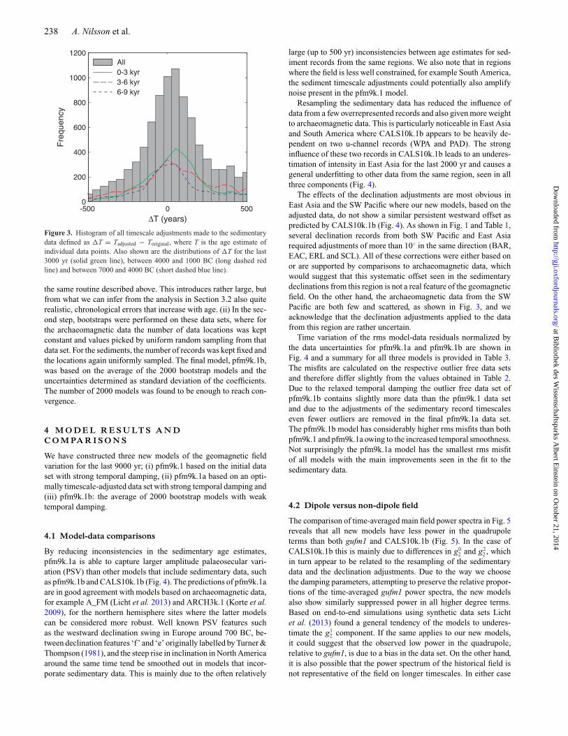
In Fig. 7, we compare time-averages/time-slices of Br at the CMBfor pfm9k.1a, pfm9k.1b and the most recent global models for threedifferent time-periods. The structures shown by the new models andCALS10k.1b are similar for the long-term time-average, 7000 BCto 1900 AD (Fig. 7a). All three models show two high latitude areasthat preferentially exhibit high intensity flux in the southern hemi-sphere, beneath South America and the Pacific Ocean, although thelatter feature is slightly less pronounced in pfm9k.1b. In addition,both pfm9k.1a and pfm9k.1b show indications of two persistenthigh latitude high intensity flux patches in northern hemisphere,beneath Greenland and Western Russia. The northern and southernhemisphere high latitude flux patches are not symmetrically locatedaround the equator. However, due to the poor data coverage for thesouthern hemisphere, the location of these flux patches are moreuncertain. As pointed out by Licht et al. (2013), and as we will seein Section 5, there is a risk that the occurrence of these features

is related to a sampling bias. The new models show a less pro-nounced SW pacific anomaly compared to CALS10k.1b due to thedeclination adjustments and the resampling of the sedimentary data.The persistent anomaly also has a different signature compared toCALS10k.1b, characterized by comparatively weaker flux beneaththe Fiji islands.

The new models’ time-averaged Br for the last 3000 yr are charac-terized by more variable field structure in the northern hemispherecompared to the longer time average (Fig. 7b). There are three areasthat preferentially exhibit high intensity fluxes beneath Greenland,Europe and Eastern Asia. Both pfm9k.1a and pfm9k.1b also exhibitgenerally more complex structure at high latitudes in the north-ern hemisphere compared to the recently published ASDI_FM-Mmodel (Licht et al. 2013). The SW Pacific anomaly is again not aspronounced in the new models compared to both in CALS10k.1band ASDI_FM-M, due to the above-mentioned adjustments of thesedimentary data. Instead the new models predict a persistent strongflux beneath East Asia.

Fig. 7(c) shows the Br prediction at the CMB of the two models forthe year 1900 AD compared to the prediction of gufm1. The northernhemisphere predictions of both models are relatively accurate butsmoothed, roughly equivalent to the gufm1 model prediction trun-cated at spherical harmonic degree 5–6 (see Fig. 8). The southernhemisphere reconstruction, on the other hand, provides much lesshigher order structure and is dominated by spherical harmonic de-gree 3–4. The two southern hemisphere high latitude high intensityflux patches present in gufm1 are represented as one diffuse area ofhigh flux in pfm9k.1a. The comparison provides a direct, althoughslightly limited, evaluation of how much structure we can expectthe models to capture. We note that sedimentary palaeomagneticdata, which are particularly important for the southern hemispherereconstruction, are poorly represented in the last few centuries ofthe database, mainly due to the difficulty in getting a reliable signalfrom the top sloppy part of sediment cores.

Fig. 9 shows five different time slices of the pfm9k.1a Br atthe CMB. We focus on the last 4000 yr where the model is bestconstrained. For a more complete illustration the reader is re-ferred to the animations provided with the Supporting Information(Movies 1–3). Throughout the selected time period the southernhemisphere Br prediction is characterized by the appearance and dis-appearance of two high latitude high intensity flux patches beneath

at Bibliothek des W




ownloaded from



Figure 6. (a) North geomagnetic pole (NGP) latitude, (b) NGP longitude, (c) dipole moment and (d) sum of non-dipole field power of the dipole field prior(dashed black line), CALS10k.1b (dashed blue line), pfm9k.1 (green line), pfm9k.1b (grey line) and pfm9k.1a (red line). Uncertainty estimates from thebootstraps of CALS10k.1b (blue) and pfm9k.1b (grey) for NGP latitude and dipole moment are shown as light shaded areas. Note that some of the jumps inthe NGP longitude, due to the circularity of the data, have been removed to make the figure clearer. The following sediment records were selected for eachlocation (see Table 1 for full names): (a) FIS, LOU, MAR, (b) CAM, ESC, MNT, TRE, (c) AD1, AD2, ANN, BEG, BOU, EIF, FRG, FUR, GEI, LOM, MEE,MEZ, MOR, MOT, NAU, POH, SAR, SAV, TY1, TY2, WIN, (d) BI2, BIW, ERL, FAN, WPA, (e) BLM, GNO, KEI.

South America and the SW Pacific. There is not much movementbetween them and for the most part they are situated at the edge ofthe tangent cylinder. The Br prediction for the northern hemispherereveals a much more dynamic behaviour. The northern hemispherestructure is dominated by the presence of two, but sometimes three,high latitude high intensity flux patches which move with an over-all westward motion around the edge of the tangent cylinder. Themovement or disappearance/emergence of flux patches is heavilysmoothed due to the strong temporal damping but appears to de-scribe a stop-and-go motion with an average rate equivalent to a5000-yr rotation period. The apparent westward high latitude fluxmotion correlates well with a more or less continuous westwardmovement of the NGP between −1800 and 600 AD (Fig. 6). TheNGP then moves eastwards up to about 500 AD during which thehigh latitude flux motion breaks down and the field structure be-comes more complex.

The field evolution at the CMB predicted by pfm9k.1a, in par-ticular, also shows a recurrence of reversed (or weak) flux just

at the edge of the tangent cylinder in the northern hemispherearound −1500, −300, 700 and 1900 AD. These reversed fluxpatches appear in association with, and at the far side of, two highlatitude high intensity flux patches predominantly situated in onehemisphere. In at least two cases (−300 and 1900 AD) they seem tooriginate from the equator and move northwards towards the edgeand possibly into the tangent cylinder over a period of a few cen-turies. However, due to the truncation level of the models it may notbe possible to track any movement into the tangent cylinder (seecomparison with gufm1 at different truncation levels, Figs 7–8).

5 E VA LUAT I O N O F M O D E L S U S I N Gg u f m 1

To investigate how well we can expect our models to resolve thefield structure at the CMB we generated a set of synthetic data setswith the same data uncertainties and the same ST data distributionas the final outlier free pfm9k.1 data set. The synthetic data sets

at Bibliothek des W




ownloaded from



Figure 7. (Upper panel) Time-averaged radial component of the field (Br) at the core mantle boundary (CMB) predicted by representative models for eachtime period: (a) CALS10k.1b 7000 BC to 1900 AD, (b) ASDI_FM 1000 BC to 1900 AD and (c) gufm1 1900 AD. Br predictions over the same time periodsfor pfm9k.1a (middle panel) and pfm9k.1b (lower panel). The dashed white lines show the CMB expression (∼71◦ N/S) of the inner core tangent cylinder.

were resampled in time and space from a reasonably realistic fielddescription, a reference field model, covering the investigated timeinterval. MA data uncertainties were added in the same way asfor the construction of pfm9k.1b, but with the distinction that thedata age estimates were kept constant and age uncertainties wereintroduced to obtain the reference field model predictions. Finally,a new set of synthetic models was produced based on the syntheticdata sets and the same damping parameters as for the final pfm9k.1model. The model performance was evaluated by comparing the Br

at the CMB of the synthetic model and the reference field model.The choice of a suitable reference field model is important and

will to some degree influence the results. For a similar type of anal-ysis Licht et al. (2013) used a periodically extended version of thegufm1 model, covering the last three millennia. Here, we have in-stead opted to use single time-slices, also derived from the gufm1model, extended back in time by adding a continuous 5000-yr west-ward rotation to the whole field. The advantage of this approach isthat it provides a direct test of the robustness of the observed west-ward drift pattern observed in the palaeofield models. An initialreference field model was constructed using the gufm1 predictionat 1840 AD and extended backwards and forwards in time with acontinuous westward rotation to cover the palaeofield model timeperiod −7000 to 1900 AD. An animation showing the time variationof the Br at the CMB for this reference field model and the corre-sponding synthetic model is provided in the Supporting Information(Movie 4).

Because of the nature of the regularization, to minimize fieldstructure at the CMB, the model performance test will be more sen-sitive in areas where the reference field model shows more struc-ture, for example in the vicinity of high intensity flux patches. Toreduce the impact of such ST differences in a particular reference

field model we generated 1000 different reference field models andcorresponding synthetic data sets. Each reference field model wasconstructed by randomly (i) varying the year (1590–1990 AD) usedto select the initial gufm1 time-slice, (ii) pre-rotating the field by0–359◦ around the z-axis and (iii) occasionally reversing the polar-ity of the field solution before extending it backwards and forwardsin time by adding the continuous westward rotation. 1000 solutionswere found to be enough to reach convergence for the time-averagedBr residuals. The rms of the Br residuals at the CMB calculated forall 1000 different cases and for every 50 yr between 7000 BC and1900 AD is shown in Fig. 10.

Not surprisingly the largest rms Br residuals are observed at highlatitudes, particularly in the Southern hemisphere beneath Africaand the Pacific, related to the occurrence of high intensity fluxpatches. The least difference is observed at mid-latitudes around thenorthern hemisphere and beneath South America and the SW Pacificwhere the data distribution is most dense. The low misfit recordedat very high latitudes in the Northern hemisphere is probably acombination of little temporal variability in the reference modeldue to the rotation around the Earth’s axis and the fact that theavailable data, in particular field intensity, sample the field quitewell at the CMB, where we apply our regularization (see fig. 1 ofKorte et al. 2011).

Comparing the temporal variability of the initial reference fieldmodel (for 1840 AD) to the corresponding synthetic model showsthat the synthetic model is able to capture both high latitude highintensity flux patches in the northern hemisphere throughout themodel time period. For the most part, however, the model onlyresolves one diffuse high intensity flux patch in the southern hemi-sphere. This is partially due to the location of the southern hemi-sphere flux patches in gufm1 for 1840 AD being situated close to

at Bibliothek des W




ownloaded from



Figure 8. Comparison of the radial component of the field (Br) at the coremantle boundary (CMB) predicted by gufm1 truncated at (a) degree lmax = 6,(b) degree lmax = 5, (c) degree lmax = 4 and (d) degree lmax = 3. The dashedwhite lines show the CMB expression (∼71◦ N/S) of the inner core tangentcylinder.

each other. If we change the polarity of the reference model (gufm1at 1840 AD) the synthetic model will at times resolve two southernhemisphere flux patches, but usually only when these are locatedbeneath South America and the SW Pacific where there the datadistribution is denser (see animation provided in the SupportingInformation, Movie 5). This implies that we cannot discriminatebetween longitudinal drift and growing/weakening flux patches inthe southern hemisphere, and even the long-term average persis-tence of flux patches could be a product of sampling bias.

A similar type of stop-and-go behaviour of the northern hemi-sphere high latitude flux patches observed in the palaeofield modelscan be observed in the synthetic models as well, although not to thesame degree. This suggests that some of the stop-and-go behaviourcould be an effect of the age uncertainties of the data, particularlythe correlated uncertainties of the sedimentary data. There is alsoa tendency of flux patches seemingly appearing, or growing in in-tensity, as they pass beneath areas with a denser data distribution(as with the southern hemisphere comparison), suggesting that theuneven geographical data distribution could also produce a similareffect.

Fig. 11 shows time-longitude plots of all three new models andthe initial synthetic model (gufm1 at 1840 AD) based on the radialfield prediction for the latitude 60◦N. In order to emphasize az-imuthal structure of the field we also show time-longitude plots after

removing the time-averaged axisymmetric part of the field (Finlay &Jackson 2003). The westward drift of the high latitude flux patchesin the northern hemisphere, noted earlier, is visible for the greaterpart of the last 4000 yr and looks fairly similar to the artificiallyinduced drift of the synthetic model. Interestingly this pattern doesnot extend further back in time in the palaeofield models, but ratherthere is a hint of persistent flux patches around −60◦ and 60◦, andpossibly also around 180◦ E, as seen in the long-term time-averagedfield (Fig. 6). The presence of the westward drift in the syntheticmodel throughout the model time period suggests that lack of driftin earlier part in palaeofield models is not due to problems with datadistribution and/or uncertainties, but a real feature of the field.

5 C O N C LU S I O N S

The pfm9k spherical harmonic models represent a new family oflow temporal resolution Holocene global geomagnetic field recon-structions. These are intended as alternatives to the widely usedCALS10k.1b, covering the same time interval, but also as com-plements to higher temporal resolution field models covering thelast three millennia such as ARCH3k.1, CALS3k.4, A_FM andASDI_FM.

All three new models show evidence for persistent high latitudehigh intensity flux at the CMB beneath Greenland, Western Russia,South America and the Pacific Ocean (Fig. 7). However, compar-isons with models constrained from synthetic data sets show clearlimitations of these predictions for high latitudes in the southernhemisphere. One of the most striking features of the time evolutionof the field at the CMB, predicted by all three new models, is adominant westward motion of northern high latitude high intensityflux patches around the edge of the tangent cylinder during thelast 4000 yr. These results are in contrast to similar studies whereboth westward and eastward drift has been observed to be moreor less equally common over the same time period (Dumberry &Finlay 2007; Wardinski & Korte 2008; Amit et al. 2011). We findthat a combination of the increased weight given to intensity data,which preferentially samples higher latitudes at the CMB (Johnson& McFadden 2007), and the inclusion of high latitude sedimentarydeclination data (Barletta et al. 2008; Lise-Pronovost et al. 2009)are important for tracking the motion of these high latitude fluxpatches. The new models also show intermittent occurrences of re-versed flux at the edge of or inside the tangent cylinder, possiblyoriginating from the equator, but further investigations are requiredto determine how robust these features are.

The new models are based on essentially the same data asCALS10k.1b but introduce new ways of treating the data, par-ticularly sedimentary data. These include redistributing the weightgiven to different sources and types of data during the inversion aswell as addressing their chronologic uncertainties in a novel way.We find that the single most important change is the resamplingof the sedimentary data, effectively reducing the influence of a fewindividual records that dominated the field reconstructions for someregions of the world, but also reassigning more weight to archaeo-magnetic data and data based on more measurements. In futurestudies, more comprehensive approaches could be used to furtherdistinguish between records based on sedimentation rates and qual-ity estimates such as the scatter of data from different independentlyoriented cores (Nilsson et al. 2010; Panovska et al. 2012).

Appropriately treating the sedimentary declination data as rel-ative values has a large impact on the final model outcome, par-ticularly for regions such as the SW Pacific where the models are

at Bibliothek des W




ownloaded from



Figure 9. Radial component of the field (Br) at the core mantle boundary (CMB) of pfm9k.1a at (a) 1200 AD, (b) 600 AD, (c) 0 AD, (d) 600 BC and (e) 1500BC. Southern hemisphere (left) and northern hemisphere (right) orthographic projections added for clarity. The dashed white lines show the CMB expression(∼71◦ N/S) of the inner core tangent cylinder.

Figure 10. The rms radial field component (Br) residuals at the core mantleboundary (CMB) between 1000 different reference field models and modelsconstrained by associated synthetic data sets for every 50 yr between 7000BC and 1900 AD (see text for a more detailed description). The dashedwhite lines show the CMB expression (∼71◦ N/S) of the inner core tangentcylinder.

dominantly constrained by sedimentary data. As discussed inSection 4.2 the adjustments used here may have led to a slighttransfer of power from higher degrees into the dipole component.We conclude that adjustments to the declination data are necessarybut that the methodology could be improved. Similar adjustmentsmay also be appropriate for the sedimentary inclination data, whichin a few cases appear to be systematically offset by more than 10◦

based on comparisons with archaeomagnetic data. Like Panovskaet al. (2012) we did not observe any systematic evidence of inclina-tion shallowing and decided against adjusting the inclination data toavoid removing real persistent non-dipolar features. We note, how-ever, that just by resampling the data most erratic offsets in either(un-adjusted) declination or inclination were successfully identifiedand removed as outliers by the modelling procedure.

One of the main problems associated with geomagnetic fieldmodelling using sedimentary palaeomagnetic data are the largeand often unknown age uncertainties. In the most recent modelling

at Bibliothek des W




ownloaded from



Figure 11. Time Longitude plots of the radial field component (Br) at the core mantle boundary (CMB) for all three new models and a synthetic model (basedon the gufm1 at 1840 AD, see text for more details) centred around 60◦N before (upper panel) and after removal of the time-averaged axisymmetric part of thefield (lower panel).

efforts this problem has been approached by bootstrap resamplingof the data set, see Section 3.3, whereby one part consists of shiftingthe whole chronology of each sedimentary record randomly in timeby a fixed value of ±300 yr (Korte et al. 2009) or using the smallerpublished age uncertainties (Licht et al. 2013). Here we have in-stead introduced an alternative, and arguably more realistic, wayof adjusting the sediment data chronologies by randomly stretchingand compressing the individual timescales of each record. Usingthis technique we have both been able to assess the likely rangeof age uncertainties, often up to and most likely also exceeding500 yr, and adjust the timescale of each record based on compar-isons with predictions from pfm9k.1. There are obvious limitationswith the methodology applied here, mainly the implicit assump-tion that the pfm9k.1 is free of chronologic errors. Yet, the resultsdemonstrate the potential information stored in sedimentary data,which can be recovered using the stratigraphic information providedwith each record. Temporal smoothing and time-lag related to lock-in processes may also be important but we find that chronologicuncertainties are most likely of greater concern for geomagneticfield reconstructions based on sedimentary data.

The source files for all three models, including the pfm9k.1bindividual bootstrap solutions, together with evaluation soft-ware are provided in the EarthRef.org Digital Archive (ERDA,http://www.earthref.org) by searching for the model names.

A C K N OW L E D G E M E N T S

This work was funded by the Natural Environment ResearchCouncil, UK, grant numbers NE/I013873/1 and NE/H021043/1.MK acknowledges support from grant KO 2870/4–1 of DeutscheForschungsgemeinschaft. We thank Catherine Constable and ananonymous reviewer for their constructive reviews of the originalmanuscript.

R E F E R E N C E S

Ali, M., Oda, H., Hayashida, A., Takemura, K. & Torii, M., 1999. Holocenepalaeomagnetic secular variation at Lake Biwa, central Japan, Geophys.J. Int., 136, 218–228.

Amit, H., Korte, M., Aubert, J., Constable, C. & Hulot, G., 2011. The time-dependence of intense archeomagnetic flux patches, J. geophys. Res.:Solid Earth, 116, B12106, doi:10.1029/2011JB008538.

Anson, G.L. & Kodama, K.P., 1987. Compaction-induced inclination shal-lowing of the post-depositional remanent magnetization in a syntheticsediment, Geophys. J. R. Astron. Soc., 88, 673–692.

Barletta, F., St-Onge, G., Channell, J.E.T. & Rochon, A., 2010. Dating ofHolocene western Canadian Arctic sediments by matching paleomagneticsecular variation to a geomagnetic field model, Quat. Sci. Rev., 29, 2315–2324.

Barletta, F., St-Onge, G., Channell, J.E.T., Rochon, A., Polyak, L. & Darby,D., 2008. High-resolution paleomagnetic secular variation and relativepaleointensity records from the western Canadian Arctic: implication forHolocene stratigraphy and geomagnetic field behaviour, Can. J. EarthSci., 45, 1265–1281.

Barton, C.E. & McElhinny, M.W., 1981. A 10 000 yr geomagnetic secularvariation record from three Australian maars, Geophys. J. Int., 67, 465–485.

Barton, C.E. & Torgersen, T., 1988. Palaeomagnetic and 210Pb estimates ofsedimentation in Lake Turkana, East Africa, Palaeogeogr. Palaeoclimatol.Palaeoecol., 68, 53–60.

Bjorck, S. & Wohlfarth, B., 2001. 14C chronostratigraphic techniques inpaleolimnology, Tracking Environmental Change Using Lake Sediments,pp. 205–245, Kluwer.

Bleil, U. & Dillon, M., 2008. Holocene Earth’s magnetic field variationsrecorded in marine sediments of the NW African continental margin,Studia Geophysica et Geodaetica, 52, 133–155.

Blow, R.A. & Hamilton, N., 1978. Effect of compaction on the acquisitionof a detrital remanent magnetization in fine-grained sediments, Geophys.J. R. Astron. Soc., 52, 13–23.

Bloxham, J., Gubbins, D. & Jackson, A., 1989. Geomagnetic secular varia-tion, Philos. Trans. R. Soc. Lond. A, 329, 415–502.

at Bibliothek des W




ownloaded from

http://www.earthref.org



Bloxham, J. & Jackson, A., 1992. Time-dependent mapping of the magneticfield at the core-mantle boundary, J. geophys. Res.: Solid Earth, 97,19 537–19 563.

Brachfeld, S.A. & Banerjee, S.K., 2000. A new high-resolution geomag-netic relative paleointensity record for the North American Holocene: acomparison of sedimentary and absolute intensity data, J. geophys. Res.,105, 821–834.

Brachfeld, S., Acton, G.D., Guyodo, Y. & Banerjee, S.K., 2000. High-resolution paleomagnetic records from Holocene sediments from thePalmer Deep, Western Antartic Peninsula, Earth planet. Sci. Lett., 181,429–441.

Brown, H., 1981. A palaeomagnetic, geochronological and palaeoenviron-mental investigation of late post glacial maar lake sediments from NWEurope, PhD thesis, University of Edinburgh, Edinburgh.

Channell, J.E.T., Hodell, D.A. & Lehman, B., 1997. Relative geomagneticpaleointensity and δ18O at ODP Site 983 (Gardar Drift, North Atlantic)since 350 ka, Earth planet. Sci. Lett., 153, 103–118.

Chaparro, M.A.E., Bohnel, H.N., Byrne, R., Nowaczyk, N.R., Molina-Garza, R.S., Park, J. & Negendank, J.F.W., 2008. Palaeomagnetic secularvariation and rock-magnetic studies of Holocene sediments from a maarlake (Hoya de San Nicolas) in Central Mexico, Geophys. J. Int., 175,462–476.

Constable, C.G., 1985. Eastern Australian geomagnetic field intensity overthe past 14000 yr, Geophys. J. R. Astron. Soc., 81, 121–130.

Constable, C.G. & McElhinny, M.W., 1985. Holocene geomagnetic secularvariation records from north-eastern Australian lake sediments, Geophys.J. Int., 81, 103–120.

Constable, C.G., Johnson, C.L. & Lund, S.P., 2000. Global geomagneticfield models for the past 3000 years: transient or permanent flux lobes?,Philos. Trans. R. Soc. Lond. A, 358, 991–1008.

Creer, K.M., Readman, P.W. & Papamarinopoulos, S., 1981. Geomagneticsecular variations in Greece through the last 6000 years obtained fromlake sediment studies, Geophys. J. Int., 66, 193–219.

Creer, K.M., Valencio, D.A., Sinito, A.M., Tucholka, P. & Vilas, J.F.A.,1983. Geomagnetic secular variations 0–14 000 yr BP as recorded bylake sediments from Argentina, Geophys. J. R. Astron. Soc., 74, 199–221.

Donadini, F., Korhonen, K., Riisager, P. & Pesonen, L.J., 2006. Database forHolocene geomagnetic intensity information, EOS, Trans. Am. geophys.Un., 87, 137–138.

Donadini, F., Korte, M. & Constable, C.G., 2009. Geomagnetic field for0–3 ka: 1. New data sets for global modeling, Geochem. Geophys.Geosyst., 10, Q06007, doi:10.1029/2008GC002295.

Doner, L., 2003. Late-Holocene paleoenvironments of northwest Icelandfrom lake sediments, Palaeogeogr. Palaeoclimatol. Palaeoecol., 193, 535–560.

Dumberry, M. & Bloxham, J., 2006. Azimuthal flows in the Earth’s coreand changes in length of day at millennial timescales, Geophys. J. Int.,165, 32–46.

Dumberry, M. & Finlay, C.C., 2007. Eastward and westward drift of theEarth’s magnetic field for the last three millennia, Earth planet. Sci. Lett.,254, 146–157.

Finlay, C.C. & Jackson, A., 2003. Equatorially dominated magnetic fieldchange at the surface of Earth’s core, Science, 300, 2084–2086.

Fisher, R., 1953. Dispersion on a sphere, Proc. R. Soc. Lond, Ser. A, 217,295–305.

Frank, U., 2007. Palaeomagnetic investigations on lake sediments from NEChina: a new record of geomagnetic secular variations for the last 37 ka,Geophys. J. Int., 169, 29–40.

Frank, U., Nowaczyk, N.R., Negendank, J.F.W. & Melles, M., 2002a. Apaleomagnetic record from Lake Lama, northern Central Siberia, Phys.Earth planet. Inter., 133, 3–20.

Frank, U., Schwab, M.J. & Negendank, J.F.W., 2002b. A lacustrine record ofpaleomagnetic secular variations from Birkat Ram, Golan Heights (Israel)for the last 4400 years, Phys. Earth planet. Inter., 133, 21–34.

Frank, U., Schwab, M.J. & Negendank, J.F.W., 2003. Results of rock mag-netic investigations and relative paleointensity determinations on lacus-trine sediments from Birkat Ram, Golan Heights (Israel), J. geophys. Res.:Solid Earth, 108, 2379, doi:10.1029/2002JB002049.

Frank, U., Nowaczyk, N.R. & Negendank, J.F.W., 2007. Palaeomagnetismof greigite bearing sediments from the Dead Sea, Israel, Geophys. J. Int.,168, 904–920.

Gallet, Y., Hulot, G., Chulliat, A. & Genevey, A., 2009. Geomagnetic fieldhemispheric asymmetry and archeomagnetic jerks, Earth planet. Sci.Lett., 284, 179–186.

Geiss, C.E., Dorale, J.A. & Dahms, D., 2007. A rockmagnetic and palaeo-magnetic record of two glacial lakes in the Wind River Range, Wyoming,USA, EOS, Trans. Am. geophys. Un., Abstract GP53B-1216.

Genevey, A., Gallet, Y., Constable, C.G., Korte, M. & Hulot, G., 2008.ArcheoInt: an upgraded compilation of geomagnetic field intensitydata for the past ten millennia and its application to the recoveryof the past dipole moment, Geochem. Geophys. Geosyst., 9, Q04038,doi:10.1029/2007GC001881.

Gogorza, C.S.G., Sinito, A.M., Lirio, J.M., Nunez, H., Chaparro, M. & Vilas,J.F., 2002. Paleosecular variations 0–19,000 years recorded by sedimentsfrom Escondido Lake (Argentina), Phys. Earth planet. Inter., 133, 35–55.

Gogorza, C.S.G., Lirio, J.M., Nunez, H., Chaparro, M., Bertorello, H.R.& Sinito, A.M., 2004. Paleointensity studies on Holocene-Pleistocenesediments from lake Escondido, Argentina, Phys. Earth Planet. Inter.,145, 219–238.

Gogorza, C.S.G., Irurzun, M.A., Chaparro, M.A.E., Lirio, J.M., Nunez,H., Bercoff, P.G. & Sinito, A.M., 2006. Relative paleointensity of thegeomagnetic field over the last 21,000 years BP from sediment cores,Lake El Trebol (Patagonia, Argentina), Earth Planets Space, 58, 1323–1332.

Gubbins, D., 1975. Can the Earth’s magnetic field be sustained by coreoscillations?, Geophys. Res. Lett., 2, 409–412.

Hagstrum, J.T. & Champion, D.E., 2002. A Holocene paleosecular varia-tion record from 14C-dated volcanic rocks in western North America,J. geophys. Res., 107, 2025, doi:10.1029/2001JB000524.

Haltia-Hovi, E., Nowaczyk, N. & Saarinen, T., 2010. Holocene palaeomag-netic secular variation recorded in multiple lake sediment cores fromeastern Finland, Geophys. J. Int., 180, 609–622.

Hayashida, A., Ali, M., Kuniko, Y., Kitagawa, H., Torii, M. & Takemura,K., 2007. Environmental magnetic record and paleosecular variation datafor the last 40 kyrs from the Lake Biwa sediments, Central Japan, EarthPlanets Space, 59, 807–814.

Hillenbrand, C.-D. et al., 2010. Age assignment of a diatomaceous oozedeposited in the western Amundsen Sea Embayment after the Last GlacialMaximum, J. Quat. Sci., 25, 280–295.

Hogg, E., 1978. The Holocene geomagnetic field in Europe, PhD thesis,University of Edinburgh, Edinburgh, U.K.

Hongre, L., Hulot, G. & Khokhlov, A., 1998. An analysis of the geomagneticfield over the past 2000 years, Phys. Earth planet. Inter., 106, 311–335.

Huttunen, P. & Stober, J., 1980. Dating of palaeomagnetic records fromFinnish lake sediment cores using pollen analysis, Boreas, 9, 193–202.

Hyodo, M. et al., 1999. A Late Holocene geomagnetic secular variationrecord from Erhai Lake, southwest China, Geophys. J. Int., 136, 784–790.

Irurzun, M.A., Gogorza, C.S.G., Chaparro, M.A.E., Lirio, J.M., Nunez,H., Vilas, J.F. & Sinito, A.M., 2006. Paleosecular variations recordedby Holocene-Pleistocene sediments from Lake El Trebol (Patagonia,Argentina), Phys. Earth planet. Inter., 154, 1–17.

Jackson, A., Jonkers, A.R.T. & Walker, M.R., 2000. Four centuries of geo-magnetic secular variation from historical records, Philos. Trans. R. Soc.Lond., A, 358, 957–990.

Johnson, C.L. & McFadden, P.L., 2007. Time-averaged field and paleosec-ular variation. in Treatise on Geophysics: Geomagnetism, vol. 5, pp.417–453, ed. Kono, M., Elsevier.

King, J.W., 1983. Geomagnetic secular variation curves for northeast-ern North America for the last 9000 years, PhD thesis, University ofMinnesota, Minneapolis.

Knudsen, M.F., Riisager, P., Donadini, F., Snowball, I., Muscheler, R.,Korhonen, K. & Pesonen, L.J., 2008. Variations in the geomagnetic dipolemoment during the Holocene and the past 50 kyr, Earth planet. Sci. Lett.,272, 319–329.

at Bibliothek des W




ownloaded from



Korhonen, K., Donadini, F., Riisager, P. & Pesonen, L.J., 2008. GEOMA-GIA50: an archeointensity database with PHP and MySQL, Geochem.Geophys. Geosyst., 9, Q04029, doi:10.1029/2007GC001893.

Korte, M. & Constable, C.G., 2003. Continuous global geomagnetic fieldmodels for the past 3000 years, Phys. Earth planet. Inter., 140, 73–89.

Korte, M. & Constable, C.G., 2005. Continuous geomagnetic field modelsfor the past 7 millennia: 2. CALS7K, Geochem. Geophys. Geosyst., 6,Q02H16, doi:10.1029/2004GC000801.

Korte, M. & Constable, C.G., 2006. On the use of calibrated relative pale-ointensity records to improve millennial-scale geomagnetic field models,Geochem. Geophys. Geosyst., 7, Q09004, doi:10.1029/2006GC001368.

Korte, M. & Constable, C., 2011. Improving geomagnetic field reconstruc-tions for 0–3 ka, Phys. Earth planet. Inter., 188, 247–259.

Korte, M. & Holme, R., 2010. On the persistence of geomagnetic flux lobesin global Holocene field models, Phys. Earth planet. Inter., 182, 179–186.

Korte, M., Genevey, A., Constable, C.G., Frank, U. & Schnepp, E., 2005.Continuous geomagnetic field models for the past 7 millennia: 1. Anew global data compilation, Geochem. Geophys. Geosyst., 6, Q02H15,doi:10.1029/2004GC000800.

Korte, M., Donadini, F. & Constable, C.G., 2009. Geomagnetic field for0–3 ka: 2. A new series of time-varying global models, Geochem. Geo-phys. Geosyst., 10, Q06008, doi:10.1029/2008GC002297.

Korte, M., Constable, C., Donadini, F. & Holme, R., 2011. Reconstructingthe Holocene geomagnetic field, Earth planet. Sci. Lett., 312, 497–505.

Lal, D., 1988. Theoretically expected variations in the terrestrial cosmic-rayproduction rates of isotopes. in Solar-Terrestrial Relationships and theEarth Environment in the last Millennia, pp. 216–233, ed. Castagnoli,G.C., North-Holland Publishing Company.

Lal, D. & Peters, B., 1967. Cosmic ray produced radioactivity on the earth,in Handbuch der Physik Band XLVI/2, pp. 551–612, Springer-Verlag.

Licht, A., Hulot, G., Gallet, Y. & Thebault, E., 2013. Ensembles of lowdegree archeomagnetic field models for the past three millennia, Phys.Earth planet. Inter., 224, 38–67.

Lifton, N., Smart, D.F. & Shea, M.A., 2008. Scaling time-integrated in situcosmogenic nuclide production rates using a continuous geomagneticmodel, Earth planet. Sci. Lett., 268, 190–201.

Lise-Pronovost, A., St-Onge, G., Brachfeld, S., Barletta, F. & Darby, D.,2009. Paleomagnetic constraints on the Holocene stratigraphy of the Arc-tic Alaskan margin, Global Planet. Change, 68, 85–99.

Lodge, A. & Holme, R., 2009. Towards a new approach to archaeomagneticdating in Europe using geomagnetic field modelling, Archaeometry, 51,309–322.

Lund, S.P. & Banerjee, S.K., 1985. Late quaternary paleomagnetic fieldsecular variation from two Minnesota Lakes, J. geophys. Res., 90, 803–825.

Mothersill, J.S., 1979. The palaeomagnetic record of the late Quaternarysediments of Thunder Bay, Can. J. Earth Sci., 16, 1016–1023.

Mothersill, J.S., 1981. Late Quaternary palaeomagnetic record of theGoderich Basin, lake Huron, Can. J. Earth Sci., 18, 448–456.

Mothersill, J., 1996. Paleomagnetic results from lakes Victoria and albert,Uganda, Studia Geophysica et Geodaetica, 40, 25–35.

Muscheler, R., Beer, J., Wagner, G., Laj, C., Kissel, C., Raisbeck, G.M.,Yiou, F. & Kubik, P.W., 2004. Changes in the carbon cycle during thelast deglaciation as indicated by the comparison of 10Be and 14C records,Earth planet. Sci. Lett., 219, 325–340.

Muscheler, R., Beer, J., Kubik, P.W. & Synal, H.A., 2005. Geomagnetic fieldintensity during the last 60,000 years based on 10Be and 36Cl from theSummit ice cores and 14C, Quat. Sci. Rev., 24, 1849–1860.

Muscheler, R., Joos, F., Beer, J., Muller, S.A., Vonmoos, M. & Snowball,I., 2007. Solar activity during the last 1000 yr inferred from radionucliderecords, Quat. Sci. Rev., 26, 82–97.

Nilsson, A., Snowball, I., Muscheler, R. & Uvo, C.B., 2010. Holocene geo-centric dipole tilt model constrained by sedimentary paleomagnetic data,Geochem. Geophys. Geosyst., 11, Q08018, doi:10.1029/2010GC003118.

Nilsson, A., Muscheler, R. & Snowball, I., 2011. Millennial scale cyclicityin the geodynamo inferred from a dipole tilt reconstruction, Earth planet.Sci. Lett., 311, 299–305.

Nurgaliev, D.K., Boisov, A.S., Heller, F., Burov, B.V., Jasonov, P.G.,Khasanov, D.I. & Ibragimov, S.Z., 1996. Geomagnetic secular variationthrough the last 3500 years as recorded by lake Aslikul sedimetns fromeastern Europe (Russia), Geophys. Res. Lett., 23, 375–378.

Nourgaliev, D.K., Heller, F., Borisov, A.S., Hajdas, I., Bonani, G., Iassonov,P.G. & Oberhansli, H., 2003. Very high resolution paleosecular variationrecord for the last ∼1200 years from the Aral Sea, Geophys. Res. Lett.,30, doi:10.1029/2003GL018145.

Nourgaliev, D.K., Heller, F., Borisov, A.C., Yasanov, P.G., Chernova, I.Y. &Hajdas, I., 2005. Principal features (master curve) of geomagnetic fieldvariations in Belorussia during the last 12 thousand years, Russ. J. EarthSci., 7, 1–16.

Ojala, A.E.K. & Saarinen, T., 2002. Palaeosecular variation of the Earth’smagnetic field during the last 10000 years based on the annually lami-nated sediment of Lake Nautajarvi, central Finland, Holocene, 12, 391–400.

Ojala, A.E.K. & Tiljander, M., 2003. Testing the fidelity of sediment chronol-ogy: comparison of varve and paleomagnetic results from Holocene lakesediments from central Finland, Quat. Sci. Rev., 22, 1787–1803.

Olson, P. & Deguen, R., 2012. Eccentricity of the geomagnetic dipole causedby lopsided inner core growth, Nature Geosci., 5, 565–569.

Panovska, S., Finlay, C.C., Donadini, F. & Hirt, A.M., 2012. Spline analysisof Holocene sediment magnetic records: uncertainty estimates for fieldmodeling, J. geophys. Res., 117, B02101, doi:10.1029/2011JB008813.

Pavon-Carrasco, F.J., Osete, M.L., Torta, J.M. & Gaya-Pique, L.R., 2009.A regional archeomagnetic model for Europe for the last 3000 years,SCHA.DIF.3K: applications to archeomagnetic dating, Geochem. Geo-phys. Geosyst., 10, Q03013, doi:10.1029/2008GC002244.

Peck, J.A., King, J.W., Colman, S.M. & Kravchinsky, V.A., 1996. An 84-kyr paleomagnetic record from the sediments of Lake Baikal, Siberia, J.geophys. Res., 101, 11 365–11 386.

Peng, L. & King, J.W., 1992. A late Quaternary geomagnetic secular vari-ation record From Lake Waiau, Hawaii, and the question of the PacificNondipole low, J. geophys. Res., 97, 4407–4424.

Richter, C., Venuti, A., Verosub, K.L. & Wei, K.-Y., 2006. Variations ofthe geomagnetic field during the Holocene: relative paleointensity andinclination record from the West Pacific (ODP Hole 1202B), Phys. Earthplanet. Inter., 156, 179–193.

Roberts, A.P. & Winklhofer, M., 2004. Why are geomagnetic excursionsnot always recorded in sediments? Constraints from post-depositionalremanent magnetization lock-in modelling, Earth planet. Sci. Lett., 227,345–359.

Saarinen, T., 1998. High-resolution palaeosecular variation in northernEurope during the last 3200 years, Phys. Earth planet. Inter., 106, 299–309.

Skilling, J., 2006. Nested sampling for general Bayesian computation.Bayesian Anal., 1, 833–860.

Snowball, I. & Muscheler, R., 2007. Palaeomagnetic intensity data: anAchilles heel of solar activity reconstructions, Holocene, 17, 851–859.

Snowball, I. & Sandgren, P., 2002. Geomagnetic field variations in northernSweden during the Holocene quantified from varved lake sediments andtheir implications for cosmogenic nuclide production rates, Holocene, 12,517–530.

Snowball, I. & Sandgren, P., 2004. Geomagnetic field intensity changesin Sweden between 9000 and 450 cal BP: extending the record of “ar-chaeomagnetic jerks” by means of lake sediments and the pseudo-Thelliertechnique, Earth planet. Sci. Lett., 227, 361–376.

Snowball, I., Zillen, L., Ojala, A., Saarinen, T. & Sandgren, P., 2007. Fennos-tack and Fennorpis: Varve dated Holocene palaeomagnetic secular vari-ation and relative palaeointensity stacks for Fennoscandia, Earth planet.Sci. Lett., 255, 106–116.

St-Onge, G., Stoner, J.S. & Hillaire-Marcel, C., 2003. Holocene paleomag-netic records from the St. Lawrence Estuary, eastern Canada: centennial-to millennial-scale geomagnetic modulation of cosmogenic isotopes,Earth planet. Sci. Lett., 209, 113–130.

St-Onge, G., Mulder, T., Piper, D.J.W., Hillaire-Marcel, C. & Stoner, J.S.,2004. Earthquake and flood-induced turbidites in the Saguenay Fjord

at Bibliothek des W




ownloaded from



(Quebec): a Holocene paleoseismicity record, Quat. Sci. Rev., 23, 283–294.

Stockhausen, H., 1998. Geomagnetic palaeosecular variation (0–13 000 yrBP) as recorded in sediments from three maar lakes from the West Eifel(Germany), Geophys. J. Int., 135, 898–910.

Stoner, J.S., Jennings, A., Kristjansdottir, G.B., Dunhill, G., Andrews, J.T.& Hardardottir, J., 2007. A paleomagnetic approach toward refiningHolocene radiocarbon-based chronologies: paleoceanographic recordsfrom the north Iceland (MD99–2269) and east Greenland (MD99–2322)margins, Paleoceanography, 22, PA1209, doi:10.1029/2006PA001285.

Suttie, N., Holme, R., Hill, M.J. & Shaw, J., 2011. Consistent treatment oferrors in archaeointensity implies rapid decay of the dipole prior to 1840,Earth planet. Sci. Lett., 304, 13–21.

Tauxe, L., 2005. Inclination flattening and the geocentric axial dipole hy-pothesis, Earth planet. Sci. Lett., 233, 247–261.

Thompson, R. & Turner, G.M., 1985. Icelandic Holocene palaeolimnomag-netism, Phys. Earth planet. Inter., 38, 250–261.

Thouveny, N. & Williamson, D., 1988. Palaeomagnetic study of theHolocene and Upper Pleistocene sediments from Lake Barombi Mbo,Cameroun: first results, Phys. Earth planet. Inter., 52, 193–206.

Turner, G.M., 1987. A 5000 year geomagnetic palaeosecular variation recordfrom western Canada, Geophys. J. R. Astron. Soc., 91, 103–121.

Turner, G.M. & Lillis, D.A., 1994. A palaeomagnetic secular variation recordfor New Zealand during the past 2500 years, Phys. Earth planet. Inter.,83, 265–282.

Turner, G.M. & Thompson, R., 1979. Behaviour of the earth’s magneticfield as recorded in the sediment of Loch Lomond, Earth planet. Sci.Lett., 42, 412–426.

Turner, G.M. & Thompson, R., 1981. Lake sediment record of the geomag-netic secular variation in Britain during Holocene times, Geophys. J. Int.,65, 703–725.

Valet, J.-P., Herrero-Bervera, E., Le Mouel, J.-L. & Plenier, G., 2008. Secularvariation of the geomagnetic dipole during the past 2000 years, Geochem.Geophys. Geosyst., 9, Q01008, doi:10.1029/2007GC001728.

Verosub, K.L., Mehringer, P.J. & Waterstraat, P., 1986. Holocene secularvariation in Western North America: paleomagnetic record from FishLake, Harney County, Oregon, J. geophys. Res., 91, 3609–3623.

Vigliotti, L., 2006. Secular variation record of the Earth’s magnetic fieldin Italy during the Holocene: constraints for the construction of a mastercurve, Geophys. J. Int., 165, 414–429.

Vonmoos, M., Beer, J. & Muscheler, R., 2006. Large variations in Holocenesolar activity: constraints from 10Be in the Greenland Ice Core Project icecore, J. geophys. Res., 111, A10105, doi:10.1029/2005JA011500.

Wardinski, I. & Korte, M., 2008. The evolution of the core-surface flowover the last seven thousands years, J. geophys. Res.: Solid Earth, 113,B05101, doi:10.1029/2007JB005024.

Weeks, R., Laj, C., Endignoux, L., Fuller, M., Roberts, A., Manganne, R.,Blanchard, E. & Goree, W., 1993. Improvements in long-core measure-ment techniques: applications in palaeomagnetism and palaeoceanogra-phy, Geophys. J. Int., 114, 651–662.

Yang, X., Heller, F., Yang, J. & Su, Z., 2009. Paleosecular variations since∼9000 yr BP as recorded by sediments from maar lake Shuangchiling,Hainan, South China, Earth planet. Sci. Lett., 288, 1–9.

Zillen, l., 2003. Setting the Holocene clock using varved lake sediments inSweden, LUNDQUA PhD thesis, Lund University, Lund.

S U P P O RT I N G I N F O R M AT I O N

Additional Supporting Information may be found in the online ver-sion of this article:

Movie 1. Radial component of the field (Br) at the core mantleboundary (CMB) predicted by pfm9k.1 between 7000 BC and 1900AD. The white lines show the CMB expression (∼71◦ N/S) of theinner core tangent cylinder.Movie 2. Radial component of the field (Br) at the core mantleboundary (CMB) predicted by pfm9k.1a between 7000 BC and1900 AD. The white lines show the CMB expression (∼71◦ N/S) ofthe inner core tangent cylinder.Movie 3. Radial component of the field (Br) at the core mantleboundary (CMB) predicted by pfm9k.1b between 7000 BC and1900 AD. The white lines show the CMB expression (∼71◦ N/S) ofthe inner core tangent cylinder.Movie 4. Radial component of the field (Br) at the core mantleboundary (CMB) of a reference field model (Upper panel) and asynthetic model (Lower panel) based on data resampled from thereference field (see text for more information). The reference fieldmodel is based on the gufm1 prediction at 1840 AD extended back-wards and forwards in time with a continuous westward rotation.The white lines show the CMB expression (∼71◦ N/S) of the innercore tangent cylinder.Movie 5. Radial component of the field (Br) at the core man-tle boundary (CMB) of a reference field model (Upper panel)and a synthetic model (Lower panel) based on data resampledfrom the reference field (see text for more information). Thereference field model is based on the gufm1 prediction at 1840AD with reversed polarity and extended backwards and forwardsin time with a continuous westward rotation. The white linesshow the CMB expression (∼l71◦ N/S) of the inner core tangentcylinder (http://gji.oxfordjournals.org/lookup/suppl/doi:10.1093/gji/ggu120/-/DC1)

Please note: Oxford University Press is not responsible for the con-tent or functionality of any supporting materials supplied by theauthors. Any queries (other than missing material) should be di-rected to the corresponding author for the article.

at Bibliothek des W




ownloaded from

http://gji.oxfordjournals.org/lookup/suppl/doi:10.1093/gji/ggu120/-/DC1

http://gji.oxfordjournals.org/lookup/suppl/doi:10.1093/gji/ggu120/-/DC1


Originally published as -...

Documents

Transcript of Originally published as -...