ORDER PICKING ORIENTED STORAGE ASSIGNMENT PROBLEM …

ORDER PICKING ORIENTED STORAGE ASSIGNMENT PROBLEM IN AVERTICAL LIFT MODULE SYSTEM

A THESIS SUBMITTED TOTHE GRADUATE SCHOOL OF NATURAL AND APPLIED SCIENCES

OFMIDDLE EAST TECHNICAL UNIVERSITY

BY

BURAK ÖZ

IN PARTIAL FULFILLMENT OF THE REQUIREMENTSFOR

THE DEGREE OF MASTER OF SCIENCEIN

INDUSTRIAL ENGINEERING

DECEMBER 2019

Approval of the thesis:


submitted by BURAK ÖZ in partial fulfillment of the requirements for the degree ofMaster of Science in Industrial Engineering Department, Middle East Techni-cal University by,

Prof. Dr. Halil KalıpçılarDean, Graduate School of Natural and Applied Sciences

Prof. Dr. Yasar Yasemin SerinHead of Department, Industrial Engineering

Assist. Prof. Dr. Sakine BatunSupervisor, Industrial Engineering, METU

Prof. Dr. Haldun SüralCo-supervisor, Industrial Engineering, METU

Examining Committee Members:

Prof. Dr. Serhan DuranIndustrial Engineering, METU

Assist. Prof. Dr. Sakine BatunIndustrial Engineering, METU

Prof. Dr. Haldun SüralIndustrial Engineering, METU

Assoc. Prof. Dr. Ayse Canan SerbetciogluIndustrial Engineering, METU

Prof. Dr. Ferda Can ÇetinkayaEndüstri Mühendisligi, Çankaya Üniversitesi

Date:

I hereby declare that all information in this document has been obtained andpresented in accordance with academic rules and ethical conduct. I also declarethat, as required by these rules and conduct, I have fully cited and referenced allmaterial and results that are not original to this work.

Name, Surname: Burak Öz

Signature :

iv

ABSTRACT


Öz, BurakM.S., Department of Industrial Engineering

Supervisor: Assist. Prof. Dr. Sakine Batun

Co-Supervisor : Prof. Dr. Haldun Süral

December 2019, 123 pages

Since the advancements in technology paved the way for an increased consumer-

manufacturer interaction, companies are forced to adapt a mass customization phi-

losophy in their production operations. This philosophy requires a higher variation

of raw materials to be stored by the manufacturer to fill the customer orders on time.

However, this increased variation in the inventory will also mean increased require-

ments for the storage area. Using automated storage and retrieval systems (AS/RS)

is one way of using the volume in warehouse buildings more efficiently. By storing

trays into the shelves inside a shuttle, vertical lift modules (VLMs) are among the

AS/RSs promising more dense storage. These units can also be combined and used

as a system called "VLM Pod". Although using a VLM helps in using the volume

more efficiently, retrieval of the trays in the VLM units may take some time and cause

unwanted waits.

This study analyses a design-to-order manufacturing company’s transaction history

and discusses the factors that make the responsiveness of a warehouse important in

such an environment. Then, the throughput related VLM decisions are discussed.

v

With the help of the observations from a time study and the transaction history of the

company, various combinations of those throughput related decisions are simulated.

After these considerations, an integer linear programming model is proposed for as-

signing parts to trays and trays to shelves in VLM units. The proposed model and

its variants are used in a computational experiment on small data sets sampled from

the company’s transaction records. The optimal solutions for the small data sets are

used in a picking simulation. According to the picking simulation with the small data

sets, the proposed model yielded an average of 10% improvement in the completion

time of all pick tasks, while the number of tray retrievals during picking is reduced

by approximately 65%, compared to the current system at the analyzed company.

Keywords: vertical lift module, storage assignment, correlated item storage, mathe-

matical programming, simulation

vi

ÖZ

BIR DIKEY DEPOLAMA ÜNITESI SISTEMINDE SIPARIS TOPLAMAODAKLI ÜRÜN YERLESTIRME PROBLEMI

Öz, BurakYüksek Lisans, Endüstri Mühendisligi Bölümü

Tez Yöneticisi: Dr. Ögr. Üyesi. Sakine Batun

Ortak Tez Yöneticisi : Prof. Dr. Haldun Süral

Aralık 2019 , 123 sayfa

Teknolojideki gelismeler sayesinde artan müsteri-tedarikçi iliskileri ile firmalar gü-

nümüzde siparis usulü kitle pazarlamacılıgı yaklasımı ile üretim yapmaya zorlan-

maktadır. Bu yaklasım ile üreticiler, müsteri taleplerini zamanında karsılamak için

yüksek çesitlilikte hammadde depolamak zorunda kalmaktadır. Aynı zamanda, artan

hammadde çesitliligi, artan depo alanı ihtiyacı anlamına gelmektedir. Otomatik yer-

lestirme ve toplama sistemlerini kullanmak, ambar binalarındaki hacmi daha verimli

kullanma yöntemlerinden biridir. Bir otomatik yerlestirme ve toplama sistemi olan

dikey depolama üniteleri, tepsileri dikey bir kule içerisindeki raflara yerlestirerek yo-

gun depolama vadetmektedir. Ayrıca, bu üniteler bir arada, "Pod" adı verilen sistemler

hâlinde de kullanılabilmektedir. Dikey depolama ünitelerini kullanmak mevcut hacmi

verimli kullanmayı saglarken, bir yandan da rafların getirilmesi sırasında istenmeyen

bekleme sürelerine yol açabilir.

Bu çalısma, siparise göre tasarım yöntemi ile imalat yapan bir firmanın geçmis islem

kayıtlarını inceleyerek, benzer ortamlarda ambarların hızlı yanıt verebilirliginin öne-

mini arttıran etkenleri tartısmaktadır. Sonrasında, dikey depolama "Pod"larının çıktı

vii

performansını etkileyen kararlar tartısılmaktadır. Sistemin zaman etüdüyle elde edilen

bilgiler ve sirketin islem geçmisi yardımı ile farklı dikey depolama "Pod" kararları si-

müle edilmektedir. Elde edilen bulgulardan yararlanarak; parçaları tepsilere, tepsileri

de raf ve dikey depolama ünitelerine atayacak bir tamsayılı dogrusal programlama

modeli önerilmektedir. Önerilen model ve onun farklı biçimleri, bahsedilen firmanın

kayıtlarından örneklenen küçük veri kümeleri ile çalıstırılmıstır. Buradan elde edi-

len en iyi çözümlerin performansı, bir siparis toplama süreci simüle edilerek mevcut

sistemle kıyaslanmıs, önerilen çözümün denenen örneklerdeki islerin bitis zamanını

%10 öne çektigi ve siparis toplama sırasındaki tepsi çagırma sayısını %65 oranında

azalttıgı gözlemlenmistir.

Anahtar Kelimeler: dikey depolama ünitesi, lokasyon atama, korelasyonlu ürün de-

polama, matematik programlama, simülasyon

viii

To my family

for their support

ix

ACKNOWLEDGMENTS

First and foremost, I would like to express my gratitude to my thesis supervisors,

Assist. Prof. Dr. Sakine Batun and Prof. Dr. Haldun Süral for their continuous

support, guidance, encouragement, and patience. Besides this study, I also learned

much from them about life. I feel very privileged to have the opportunity to work

with them.

I would also like to thank the members of the examining committee, Prof. Dr. Serhan

Duran, Assoc. Prof. Dr. Ayse Canan Serbetcioglu and Prof. Dr. Ferda Can Çetinkaya

for reviewing this work and providing invaluable feedback.

It would be much more difficult for me to make this venture a success without the

people who were with me during this period. I feel immense gratitude to my dear

friends Melis Özates Gürbüz, Altan Akdogan, and Dilay Aktas for being my com-

panion. Their encouragement kept me going at those difficult times. I also appreciate

the fellowship of Engin Kut and Yılmaz Ezilmez during long study nights. I would

also like to thank Ege Erol for dedicating his valuable time for answering all my

questions about his expertise, "Vertical Lift Modules".

I also want to thank my family for all their support. Words are never going to be

enough to describe how grateful I am for them.

Above all, the things I have accomplished would not even be a possibility if my other

half, Sena Önen Öz, was not there for me. I am thankful to her for making my life

beautiful with her love, support, and encouragement.

Finally, I want to express my gratitude for the volunteers of the free and open-source

software community, especially the contributors of the Debian Project, R Core Team,

and The Document Foundation. Their efforts made this project possible!

x

TABLE OF CONTENTS

ABSTRACT . . . . . . . . . . . . . . . . . . . . . . . . . . . . . . . . . . . . v

ÖZ . . . . . . . . . . . . . . . . . . . . . . . . . . . . . . . . . . . . . . . . . vii

ACKNOWLEDGMENTS . . . . . . . . . . . . . . . . . . . . . . . . . . . . . x

TABLE OF CONTENTS . . . . . . . . . . . . . . . . . . . . . . . . . . . . . xi

LIST OF TABLES . . . . . . . . . . . . . . . . . . . . . . . . . . . . . . . . xv

LIST OF FIGURES . . . . . . . . . . . . . . . . . . . . . . . . . . . . . . . . xx

LIST OF ALGORITHMS . . . . . . . . . . . . . . . . . . . . . . . . . . . . . xxiii

LIST OF ABBREVIATIONS . . . . . . . . . . . . . . . . . . . . . . . . . . . xxiv

CHAPTERS

1 INTRODUCTION . . . . . . . . . . . . . . . . . . . . . . . . . . . . . . . 1

2 BACKGROUND INFORMATION . . . . . . . . . . . . . . . . . . . . . . 3

2.1 Vertical Lift Modules (VLMs) . . . . . . . . . . . . . . . . . . . . . 5

2.2 Analysis of a Job Shop Manufacturing Firm’s History Data & Out-comes . . . . . . . . . . . . . . . . . . . . . . . . . . . . . . . . . . 7

2.2.1 Company Overview . . . . . . . . . . . . . . . . . . . . . . . 7

2.2.2 Activity Profile of the Studied Real Life Warehouse . . . . . . 9

2.2.3 Overview of the VLM Pod in AE’s Warehouse . . . . . . . . . 10

2.2.4 Factors that Make Responsiveness of Warehouses Importantin Job Shop Environments . . . . . . . . . . . . . . . . . . . . 14

xi

2.3 Data Sources . . . . . . . . . . . . . . . . . . . . . . . . . . . . . . 16

2.3.1 Analyzed Company’s Enterprise Resource Planning Software(ERP) Database . . . . . . . . . . . . . . . . . . . . . . . . . 16

2.3.2 Time Study . . . . . . . . . . . . . . . . . . . . . . . . . . . 16

2.3.2.1 Machine Time Study . . . . . . . . . . . . . . . . . . . 16

2.3.2.2 Operator Time Study . . . . . . . . . . . . . . . . . . . 19

2.4 Motivation of the Study . . . . . . . . . . . . . . . . . . . . . . . . 20

3 PROBLEM STATEMENT . . . . . . . . . . . . . . . . . . . . . . . . . . . 23

3.1 Order Based VLM Pod Storage Assignment Problem . . . . . . . . . 24

3.2 Order Picking Location Selection in Fragmented Storage . . . . . . . 27

3.3 Other Sub Problems Related with the Throughput of a VLM Pod . . . 28

4 LITERATURE REVIEW . . . . . . . . . . . . . . . . . . . . . . . . . . . 31

4.1 Vertical Lift Modules . . . . . . . . . . . . . . . . . . . . . . . . . . 31

4.2 Storage Location Assignment . . . . . . . . . . . . . . . . . . . . . 35

4.2.1 Correlated Storage Assignment for BOM Picking . . . . . . . 36

5 MATHEMATICAL MODEL FOR THE STORAGE LOCATION ASSIGN-MENT PROBLEM . . . . . . . . . . . . . . . . . . . . . . . . . . . . . . 39

5.1 Mathematical Model for Order Based VLM Pod Storage Assignment 39

5.2 Linearized Version of Model MQP . . . . . . . . . . . . . . . . . . . 42

5.3 Relaxation of the Binary Set Constraints in MILP . . . . . . . . . . . 44

5.3.1 Relaxation of the Binary Set Constraints on mbtfsz . . . . . . . 44

5.3.2 Relaxation of the Binary Set Constraints on mbtfsz and ktfsz . 45

5.3.3 Relaxation of the Binary Set Constraints on mbtfsz, ktfsz andybts . . . . . . . . . . . . . . . . . . . . . . . . . . . . . . . . 46

xii

5.3.4 Relaxation of the Binary Set Constraints on wpbts and mbtfsz . 47

5.3.5 Relaxation of the Binary Set Constraints on mbtfsz, ktfsz, ybtsand wpbts . . . . . . . . . . . . . . . . . . . . . . . . . . . . . 48

6 COMPUTATIONAL EXPERIMENTS . . . . . . . . . . . . . . . . . . . . 49

6.1 Problem Settings and Generation of the Problem Instances . . . . . . 49

6.2 Computational Performance for the Proposed Models . . . . . . . . . 52

6.3 Quality of the Obtained Solutions . . . . . . . . . . . . . . . . . . . 60

7 CONCLUSION . . . . . . . . . . . . . . . . . . . . . . . . . . . . . . . . 73

REFERENCES . . . . . . . . . . . . . . . . . . . . . . . . . . . . . . . . . . 77

APPENDICES

A ANALYSIS OF THE MANUFACTURING COMPANY’S OPERATIONS . 83

B PROBLEM DEFINITION . . . . . . . . . . . . . . . . . . . . . . . . . . . 93

C SIMULATION OF VARIOUS VLM POD DECISIONS . . . . . . . . . . . 95

C.1 Assumptions . . . . . . . . . . . . . . . . . . . . . . . . . . . . . . 97

C.2 Outcomes of the Preliminary VLM Pod Simulations . . . . . . . . . 101

C.2.1 Impact of the Distance Between Units on the System Throughput102

C.2.2 Impact of the Storage Assignment Rule on the System Through-put . . . . . . . . . . . . . . . . . . . . . . . . . . . . . . . . 102

C.2.3 Impact of the VLM Unit Sequencing Rules on the SystemThroughput . . . . . . . . . . . . . . . . . . . . . . . . . . . 103

C.2.4 Impact of the Number of VLM Units on the System Throughput104

C.3 Conclusion for the Preliminary Order Picking Simulation . . . . . . . 105

D DISCUSSION OF THE IMPACT OF TRAY RETRIEVAL SEQUENCEON THE SYSTEM THROUGHPUT . . . . . . . . . . . . . . . . . . . . . 115

xiii

E COMPUTATIONAL EXPERIMENTS . . . . . . . . . . . . . . . . . . . . 119

xiv

LIST OF TABLES

TABLES

Table 2.1 List of the tasks of a VLM unit in a dual command operation and

their observation results in the time study. . . . . . . . . . . . . . . . . . . 19

Table 2.2 List of the tasks of the operator in a picking operation and their

observation results in the time study. . . . . . . . . . . . . . . . . . . . . 20

Table 3.1 List of current set of decisions for all the described sub problems. . . 29

Table 4.1 List of search engines used in the literature review. . . . . . . . . . . 31

Table 4.2 List of research questions used in the literature review on VLMs. . . 32

Table 4.3 List of keywords used in the literature review. Results of the last

four keywords have been investigated in terms of their proposed method’s

applicability to a VLM, since there are some common features between

VLMs and the systems given in these keywords. . . . . . . . . . . . . . . 32

Table 4.4 List of exclusion criteria used in the literature review. An answer of

"no" for at least one of these questions will lead to exclusion of a search

result from the review process. . . . . . . . . . . . . . . . . . . . . . . . 33

Table 5.1 Notation used for mathematical formulation MQP . . . . . . . . . . 40

Table 5.2 Additional notation used for mathematical formulation MILP . . . . 42

Table 6.1 Levels for the parameters defining the problem setting. . . . . . . . 50

xv

Table 6.2 Number of solved instances (nS) out of 10 instances for each setting,

using model MILP . . . . . . . . . . . . . . . . . . . . . . . . . . . . . . 53

Table 6.3 Number of solved instances out of 810 for each model. . . . . . . . 53

Table 6.4 Number of solved instances out of 10 by using models MILP−m,

MILP−mk, MILP−mky. . . . . . . . . . . . . . . . . . . . . . . . . . . . . 56

Table 6.4 Number of solved instances out of 10 by using models MILP−m,

MILP−mk, MILP−mky. . . . . . . . . . . . . . . . . . . . . . . . . . . . . 57

Table 6.5 Solution time and optimality gap values for modelsMILP ,MILP−m,

MILP−mk, MILP−mky; in each problem setting. . . . . . . . . . . . . . . . 58

Table 6.6 Solution time and optimality gap values for models MILP − w,

MILP−mw, MILP−mkwy; in each problem setting. . . . . . . . . . . . . . . 59

Table 6.7 Number of obtained optimal values from the overall experimental

runs for all used problem instances. . . . . . . . . . . . . . . . . . . . . . 60

Table 6.8 Average optimal values obtained from all experimental runs. . . . . 61

Table 6.9 Simulated scenarios in the verification phase. . . . . . . . . . . . . 62

Table 6.10 % improvements in the number of tray retrievals in Scenario 1, com-

pared with Scenario 4. . . . . . . . . . . . . . . . . . . . . . . . . . . . . 64

Table 6.11 % improvements in the number of tray retrievals in Scenario 1, com-

pared with Scenario 6. . . . . . . . . . . . . . . . . . . . . . . . . . . . . 64

Table 6.12 % improvements in the time spent walking in Scenario 1, compared

with Scenario 4. . . . . . . . . . . . . . . . . . . . . . . . . . . . . . . . 67

Table 6.13 % improvements in the time spent walking in Scenario 1, compared

with Scenario 6. . . . . . . . . . . . . . . . . . . . . . . . . . . . . . . . 67

Table 6.14 % improvements in the order picking completion times in Scenario

1, compared with 4. . . . . . . . . . . . . . . . . . . . . . . . . . . . . . 68

xvi

Table 6.15 % improvements in the order picking completion times in Scenario

1, compared with Scenario 6. . . . . . . . . . . . . . . . . . . . . . . . . 68

Table 6.16 Average order picking completion times (cmax) in the considered

scenarios. . . . . . . . . . . . . . . . . . . . . . . . . . . . . . . . . . . . 69

Table 6.17 Average operator utilization levels (Op.Util.) in the considered sce-

narios. . . . . . . . . . . . . . . . . . . . . . . . . . . . . . . . . . . . . 70

Table 6.18 Average time spent walking in the considered scenarios in seconds. . 71

Table 6.19 Average of total number of tray retrievals in each replication and in

each setting in the considered scenarios. . . . . . . . . . . . . . . . . . . 72

Table A.1 Basic aggregate descriptors of the activities done in the analyzed

VLM System. . . . . . . . . . . . . . . . . . . . . . . . . . . . . . . . . 86

Table C.1 Simulated scenarios and their parameters. * indicates the scenario

reflecting the current real life situation at the AE. . . . . . . . . . . . . . . 97

Table C.2 Individual 99 percent confidence intervals for all comparisons with

the current system (scenario 4) (µ4−µj, j = 3, 7, 8, 11, 12, 15, 16 and µi is

the mean of all cMax values for scenario i); * denotes significant difference101

Table C.3 Scenarios with 3 seconds of walk between units and their alterna-

tives with a longer walk duration. ** denotes the current system. . . . . . 102

Table C.4 Individual 99 percent confidence intervals for all comparisons be-

tween random storage assignment and turnover based storage assignment

scenarios (µi−µj, i ∈ set of scenarios with random storage, j ∈ set of sce-

narios with the same set of decisions, except with a turnover based storage

rule and µi is the mean of all cMax values for scenario i); * denotes the

cases where using turnover based storage assignments is significantly better.103

xvii


tween scenarios having different VLM unit sequencing rules: "wait for

the next tray in same VLM unit" and "walk to the other VLM unit".

(µi−µj, i ∈ set of scenarios with VLM sequencing rule as "wait", j ∈ set

of the same scenarios, except with the VLM sequencing rule as "walk". µi

is the mean of all cMax values for scenario i); * denotes the cases where

using a VLM sequencing rule as "walk" is significantly better. . . . . . . . 104


tween 2 VLM and 3 VLM scenarios (µi − µj, i ∈ set of scenarios with 2

VLMs, j ∈ set of the scenarios with the exactly same decisions, except

with 3 VLMs and µi is the mean of all cMax values for scenario i); *

denotes the cases where using 3 VLMs is significantly better, where **

denotes the cases where using 2 VLMs is significantly better in terms of

the system throughput. . . . . . . . . . . . . . . . . . . . . . . . . . . . . 105

Table C.7 cMax values for each scenario, replications from 1 to 25 in the

simulation study. . . . . . . . . . . . . . . . . . . . . . . . . . . . . . . . 107





Table C.10cMax values for each scenario, replications from 76 to 100 in the


Table C.11Operator’s utilization levels for each scenario, replications from 1

to 25 in the simulation study. . . . . . . . . . . . . . . . . . . . . . . . . 111





xviii



Table D.1 Notation used in the throughput model presented in Meller and

Klote (2004). . . . . . . . . . . . . . . . . . . . . . . . . . . . . . . . . . 116

Table E.1 Matrix representing the difficulty advancement steps used in the ex-

periments. As the indicated step numbers increase, the problems become

computationally more challenging. . . . . . . . . . . . . . . . . . . . . . 119

Table E.2 Order picking completion time (cmax), % operator utilization, time

spent walking (twalk) and number of tray retrievals in the considered sce-

narios. . . . . . . . . . . . . . . . . . . . . . . . . . . . . . . . . . . . . 122

Table E.3 Order picking completion time (cmax), % operator utilization, time

spent walking (twalk) and number of tray retrievals in the considered sce-

narios. . . . . . . . . . . . . . . . . . . . . . . . . . . . . . . . . . . . . 123

xix

LIST OF FIGURES

FIGURES

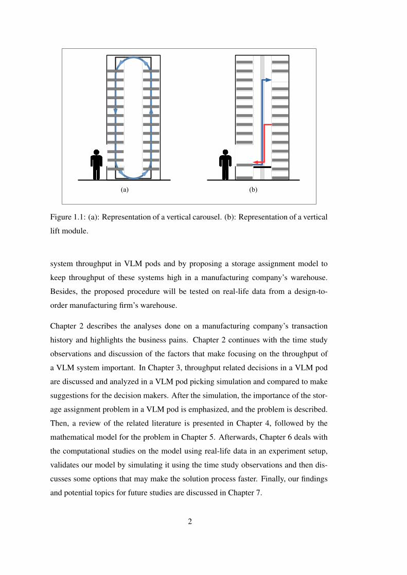
Figure 1.1 (a): Representation of a vertical carousel. (b): Representation of

a vertical lift module. . . . . . . . . . . . . . . . . . . . . . . . . . . . 2

Figure 2.1 A basic representation of the operations during a part’s life cycle

at a typical production facility’s warehouse. . . . . . . . . . . . . . . . 3

Figure 2.2 Summary of operations in a warehouse consisting of various

areas. This study focuses on activities surrounded by the dashed line. . . 4

Figure 2.3 (a): Components of a VLM unit. (b): Representation of a VLM

tray on I/O location from the operator’s perspective (Retrieved from

Romaine (2004)). . . . . . . . . . . . . . . . . . . . . . . . . . . . . . 6

Figure 2.4 A photograph of a VLM pod. Retrieved from Kardex AG (2018). 6

Figure 2.5 Product-process matrix diagram, example product and processes

based on proposed model by Hayes and Wheelwright (1979) and ana-

lyzed environment’s position (AE) on the matrix. . . . . . . . . . . . . 8

Figure 2.6 Lateness status of pick order lines by months. . . . . . . . . . . 10

Figure 2.7 Distribution of picking operations over the parts in the VLM

system. . . . . . . . . . . . . . . . . . . . . . . . . . . . . . . . . . . 13

Figure 2.8 Distribution of picking operations over trays. . . . . . . . . . . . 13

Figure 2.9 Number of processed order lines by each unit for the period

between Jan. 2018 and Mar. 2019. . . . . . . . . . . . . . . . . . . . . 14

xx

Figure 2.10 Relational schema of the database tables obtained from AE for

this study. . . . . . . . . . . . . . . . . . . . . . . . . . . . . . . . . . 17

Figure 2.11 Representation of machine tasks listed in Table 2.1. Tasks (2),

(4) and (6) are considered under the "vertical movement" categories.

(a): Tray put tasks; (b): Tray retrieval tasks. . . . . . . . . . . . . . . . 18

Figure 2.12 Summary of warehousing decisions in a VLM pod. . . . . . . . 21

Figure 3.1 Concept map representing input/output relations between the de-

fined sub problems and their environment. Note that rectangles repre-

sent decisions and circles represent outputs. . . . . . . . . . . . . . . . 24

Figure A.1 Number of released manufacturing shop orders in each month

between Jan. 2018 and Mar. 2019. In Aug. 2018, facility has been

partially closed due to maintenance operations, so the unusual behavior

is expected for Aug. 2018. . . . . . . . . . . . . . . . . . . . . . . . . 83

Figure A.2 Total number of component lines for all shop orders released in

each month. . . . . . . . . . . . . . . . . . . . . . . . . . . . . . . . . 84

Figure A.3 Number of released manufacturing and rework shop orders in

each month between Jan. 2018 and Mar. 2019. . . . . . . . . . . . . . . 84

Figure A.4 Distribution of number of locations assigned in the most active

warehouse areas. . . . . . . . . . . . . . . . . . . . . . . . . . . . . . 85

Figure A.5 Distribution of pick operations among the warehouse areas. . . . 85

Figure A.6 Monthly breakdown of number of processed order lines. . . . . . 86

Figure A.7 Distribution of picks over SKUs across the whole warehouse.

This Pareto chart justifies the current location area assignment process,

which distributes parts among different warehouse areas according to

their activity classes. . . . . . . . . . . . . . . . . . . . . . . . . . . . 87

xxi

Figure A.8 Breakdown of warehouse pick order line reasons for orders be-

tween Jan. 2018 and Mar. 2019. High ratio of shop order picks support

imply that the warehouse may benefit from a BOM based storage as-

signment method. . . . . . . . . . . . . . . . . . . . . . . . . . . . . . 87

Figure A.9 Lateness status of previous pick orders for each warehouse area. 88

Figure A.10 Locations colored according to their related final product. Each

color indicates a different final product and there is no location in this

figure that is shared by more than one final product. . . . . . . . . . . . 89

Figure A.11 Heatmap of all locations in the VLM System. Darker colors

indicate more activity. . . . . . . . . . . . . . . . . . . . . . . . . . . . 90

Figure A.12 Distribution of pick operations among the warehouse areas and

shop order disciplines. . . . . . . . . . . . . . . . . . . . . . . . . . . 91

Figure A.13 Flow chart of the pick process in "wait for the next tray" VLM

unit sequencing method. . . . . . . . . . . . . . . . . . . . . . . . . . 92

Figure B.1 Defined problem’s boundaries. . . . . . . . . . . . . . . . . . . 94

Figure C.1 VLM pod in the AE. . . . . . . . . . . . . . . . . . . . . . . . . 96

Figure D.1 Tasks in a dual cycle AS/RS operation. Tasks (1), (2) and (3)

represent putting the previous tray into its place. Operation (4) repre-

sents the empty lift’s movement from the previous tray’s location to the

next tray’s location. Finally, tasks (5), (6) and (7) represent the retrieval

of the next tray to the I/O location. . . . . . . . . . . . . . . . . . . . . 116

Figure D.2 A VLM unit with the mentioned sections (retrieved from Meller

and Klote (2004)). . . . . . . . . . . . . . . . . . . . . . . . . . . . . . 117

xxii

LIST OF ALGORITHMS

ALGORITHMS

Algorithm 1 Preliminary simulation . . . . . . . . . . . . . . . . . . . . . . 99

Algorithm 2 Function eventTimes, Time advancements and recording pick

operation event times . . . . . . . . . . . . . . . . . . . . . . . . . . . . 100

Algorithm 3 Problem instance generation . . . . . . . . . . . . . . . . . . . 120

Algorithm 4 Simulation to verify the proposed model . . . . . . . . . . . . 121

xxiii

LIST OF ABBREVIATIONS

ABBREVIATIONS

AE Analyzed environment. Refers to the manufacturing firm that

have provided its operational history data to be analyzed by the

author. Real-life problem data sets are also obtained from this

company and time studies had been conducted there.

AS/RS Automated storage and retrieval systems

BOM Bill of materials

CBS Class based storage

COI Cube-per-order index

ERP Enterprise resource planning software

I/O Input and output

LP Linear programming

SKU Stock keeping unit, refers to a distinct part type and used inter-

changeably with the word "part"

VLM Vertical lift module

xxiv

CHAPTER 1

INTRODUCTION

In recent years, increased technology usage and globalization have made the com-

petition in markets more intense. First, there is an increase in the buyers’ ability to

negotiate on the prices and reach other alternatives. Moreover, there is a trend towards

smaller lot sizes and higher customization in manufacturing operations. These factors

force companies to reduce operational costs and response times to stay in the game.

Therefore, improving productivity in warehousing operations is more important than

before (Le-Duc and de Koster, 2007).

In such market conditions, automated storage and retrieval systems (AS/RSs), such as

Vertical Carousels and Vertical Lift Modules (VLM) are becoming popular solutions

to the problem of increasing the throughput and space efficiency in warehouses (MHI,

2012).

Vertical carousels and VLMs are mini-load parts-to-picker AS/RSs where parts are pre-

sented to the picker in containers. All the containers in vertical carousels move to-

gether, whereas VLMs have a lift system that retrieves or stores containers indepen-

dently (see Figure 1.1). They both provide space efficiency compared to the tradi-

tional storage racks. However, as noted by Romaine (2004) and Jacobs et al. (2000),

throughput advantages of these systems highly depend on the storage assignments of

parts since the tray retrieval operations take a significant time and the number of tray

retrievals in a picking task depends on the storage locations of the parts.

In the literature, there are many studies about vertical and horizontal carousel systems.

However, only a few studies on VLMs exist (Dukic et al., 2015; Nicolas et al., 2018).

This study aims to fill this gap by discussing the decision alternatives impacting the

1

(a) (b)

Figure 1.1: (a): Representation of a vertical carousel. (b): Representation of a vertical

lift module.

system throughput in VLM pods and by proposing a storage assignment model to

keep throughput of these systems high in a manufacturing company’s warehouse.

Besides, the proposed procedure will be tested on real-life data from a design-to-

order manufacturing firm’s warehouse.

Chapter 2 describes the analyses done on a manufacturing company’s transaction

history and highlights the business pains. Chapter 2 continues with the time study

observations and discussion of the factors that make focusing on the throughput of

a VLM system important. In Chapter 3, throughput related decisions in a VLM pod

are discussed and analyzed in a VLM pod picking simulation and compared to make

suggestions for the decision makers. After the simulation, the importance of the stor-

age assignment problem in a VLM pod is emphasized, and the problem is described.

Then, a review of the related literature is presented in Chapter 4, followed by the

mathematical model for the problem in Chapter 5. Afterwards, Chapter 6 deals with

the computational studies on the model using real-life data in an experiment setup,

validates our model by simulating it using the time study observations and then dis-

cusses some options that may make the solution process faster. Finally, our findings

and potential topics for future studies are discussed in Chapter 7.

2

CHAPTER 2

BACKGROUND INFORMATION

Warehousing operations can be categorized as receiving, storage, picking, and ship-

ment in chronological order of occurrence (Çelik, 2009). First, materials to be stored

are received from their sources, such as manufacturing or purchasing. Then, they

are controlled according to the respective quality measures. After the quality control

step, parts are stored with respect to the warehouse’s location assignment method.

Picking activities comprise collecting the demanded items from their locations. Fol-

lowing activities, such as ensuring the correctness of collected quantities, packing

the items as ordered, and loading the vehicles are considered as shipment activities.

These operations are summarized in Figure 2.1.

Warehouse

Receiving

Purchasing

Storage Picking Shipment

Manufacturing

Figure 2.1: A basic representation of the operations during a part’s life cycle at a

typical production facility’s warehouse.

In the literature, order picking is often defined as the most demanding activity among

all warehouse operations, both in terms of cost and time (de Koster et al., 2007; Li

et al., 2017; Sgarbossa et al., 2019; Tompkins et al., 2010). Therefore, as also stated

by Frazelle (2001), order picking has great potential for increased productivity in a

3

warehouse. Moreover, the current market conditions force suppliers to reduce their

cycle times and increase the necessity of higher efficiency levels in order picking

operations.

On the other hand, the physical area is still a constraint for warehouse managers. To

use the area efficiently, warehouses generally consist of various sections with differ-

ent physical attributes, each suitable for efficient storage of a different-sized set of

parts. These sections often include traditional racks, narrow locations for small parts,

automated storage and retrieval system (AS/RS) setups. A generalized representation

of the operations in such warehouses can be seen in Figure 2.2, where a section is

dedicated to a specific AS/RS setup, Vertical Lift Module (VLM) Pod.

Receive

Manufacturing

Purchasing

Warehouse

Warehouse area

location

decisions

…

…

Area 1

Area 2

Area 3

VLM Pod

Location

assignment

inside

warehouse

area

Picking in

each

warehouse

area

Consolidation

of SKUs from

different

warehouse

areas

Shipment to

destination

Figure 2.2: Summary of operations in a warehouse consisting of various areas. This

study focuses on activities surrounded by the dashed line.

Aside from their benefits in floor space utilization, AS/RSs have advantages in reduc-

ing time spent walking in order picking times. Therefore, these systems are used by

companies to adapt their warehousing operations for today’s conditions (Dukic et al.,

2015).

VLMs, which are examples of AS/RS types, have received attention in the literature

in the recent years (Li et al., 2017). These systems can be used as a single unit, or can

be combined to form a system called a "Pod". This modularity allows the warehouse

designers to be more flexible in decisions related to storage capacity improvements.

4

In such setups, the operator is expected to be working on a unit while the other unit

is busy retrieving the next tray. However, this can be achieved if only the load distri-

bution among the units in the pod is balanced (Bozer and White, 1996). Therefore,

balancing the workloads of individual units in a pod becomes a new challenge in such

setups (Racca, 2015). Another challenge is determining the loading strategy since

the system’s picking performance depends on the storage assignment method (Jacobs

et al., 2000).

This study’s primary motivation is to focus on the highlighted operations in Figure

2.2 and provide an analysis on the operations history of a design-to-order armored

land vehicles manufacturer in Ankara. This study will present detailed information

about the environment, describe the mentioned analysis, and then make the problem

statement.

2.1 Vertical Lift Modules (VLMs)

VLMs are parts-to-picker AS/RSs where several trays are stored in a high rectangular

prism. In these systems, trays containing the requested parts are presented to the

input/output (I/O) location. Trays in a VLM are generally divided by boxes to form

individual storage locations. Once a tray is on the I/O location, the picker picks the

part from its box with the help of indicators pointing the correct box. A representation

of a VLM system can be seen in Figure 2.3. This setting is similar to end-of-aisle

mini-load AS/RSs except for having only two columns in the y-axis. Although Battini

et al. (2016) argue that VLMs are often used for storing less popular parts, warehouses

that store parts of any activity class in VLMs also exist (Gullberg and Lundberg, 2017;

Hulshof, 2019; Racca, 2015; Sinha, 2016; Tenhagen, 2018).

When the VLM units are integrated and assigned to one operator to form a "Pod", they

can be considered as a multi aisle AS/RS with as many I/O locations as the number

of VLM units forming that pod. A VLM pod’s representation can be seen in Figure

2.4. This modular approach makes capacity improvement expansions easier after the

system setup.

5

Shelf

Tray

I/OLocation

Lift

(a) (b)

Figure 2.3: (a): Components of a VLM unit. (b): Representation of a VLM tray on

I/O location from the operator’s perspective (Retrieved from Romaine (2004)).

The advantages of using a VLM setup can be listed as space savings, lower labor

costs with reduced walking distances, and increased control on the inventory on hand

(Dukic et al., 2015). VLMs also provide improvements in ergonomics, which is an

essential factor in operational success (Grosse et al., 2015). By having the I/O point

in the "Green Zone" defined by Finnsgård et al. (2011), VLMs reduce the need for

non-natural postures that may cause musculoskeletal issues during picking (Grosse

et al., 2015).

Figure 2.4: A photograph of a VLM pod. Retrieved from Kardex AG (2018).

6

2.2 Analysis of a Job Shop Manufacturing Firm’s History Data & Outcomes

As the first step of this study, an analysis of the operations record of an armored land

vehicle manufacturing plant had been made. After the analysis, it has been found

that the operational efficiency of a VLM pod in the company’s warehouse could have

been improved with the help of better decision support tools. This section will briefly

describe the manufacturing environment and present the factors that make up the

motivation of this study’s focus, increasing the throughput in a VLM pod.

2.2.1 Company Overview

In a design-to-order manufacturing company, each order can be considered as a dif-

ferent project. An increased number of customers means high marginal complexity

for such environments in many cases, because of distinct requirements on products in

each order. In addition to the wide variety in the set of products, ordered quantities

in the defense industry are low in general (Hartley, 2007; Rogerson, 1995). Being a

manufacturer of armored defense vehicles, the analyzed environment (AE) is no ex-

ception to that. Therefore, it can be an excellent example of a company on the upper

left corner of the product-process matrix defined by Hayes and Wheelwright (1979),

which is a tool that can be used to get some insights on how a company operates based

on its product and process characteristics. This matrix is shown in Figure 2.5.

Products of the AE have many different components, therefore many bill of materials

(BOM) lines. The average number of BOM lines per product is more than 6,000 for

this company. Manufacturers of similarly complex products can also be expected to

have a similarly high number of BOM lines for their products. A sampling on the

AE’s BOM tables indicated that different products in the same order had common

component ratios between 50%-90%, where the same metric was approximately 5%

between two products from different orders.

With a wide variety of complex products, AE also has many distinct components.

Among all the components in the database, AE has 73% of them defined as purchased

from a supplier. This finding is in line with the generalizations of Hartley (2007) about

the complexity of subcontractor networks in the defense industry.

7

I II III IV

Low volume, low standardization, one of a kind

Multiple products, low volume

Few major products, higher volume

High volume, high standardization, commodity products

I: Jumbled flow (job shop)

void

II: Disconnected line flow (batch)

III: Connected line flow (assembly line)

IV: Continuous flow

void

Product structure / Product lifecycle stage

Pro

cess

str

uctu

re /

Pro

cess

life

cycl

e st

age

Commercial printer

Heavy equipment

Auto assembly

Sugar refinery

AE

Figure 2.5: Product-process matrix diagram, example product and processes based

on proposed model by Hayes and Wheelwright (1979) and analyzed environment’s

position (AE) on the matrix.

Being a job shop production environment, AE has different manufacturing disci-

plines. For each production discipline’s operation, a new shop order is released. The

number of released shop orders is kept evenly in each month to utilize the production

capacity better (Figure A.1). However, since products that are being produced differ

from time to time, the total number of components requested from the warehouse

fluctuates each month (Figure A.2). This issue can be considered as the "bullwhip

effect", which is a term describing that a small change in the customer demand re-

sults in higher impacts in the upstream nodes of the supply chain Gong and de Koster

(2011).

After the manufacturing operations are completed, all products go through a series

of inspections. Some of these items are rejected and returned to manufacturing as

a component for rework shop orders. These rework shop orders create unexpected

workloads at the warehouse. Count of the rework shop orders accounted for 26% of

all released shop orders between January 2018 and March 2019. This information

supports the survey outcomes of Rawabdeh (2005), a study that lists defects among

the top issues causing unnecessary operations in job shop manufacturing firms. The

monthly breakdown of the shop orders by their types in AE (repair or manufacture)

8

can be seen in Figure A.3. This figure shows that the percentage of rework orders

stays approximately the same among the months. That is, a high number of rework

orders is a constant issue for the AE, rather than being an occasional problem. Al-

though the number of rework shop orders can be estimated, the context of these orders

cannot be known in advance. Therefore, activities in the warehouse of AE should be

flexible enough to cope with these uncertainties.

2.2.2 Activity Profile of the Studied Real Life Warehouse

To understand the warehouse in AE better and be able to present its current situation,

a warehouse activity profiling has been conducted following suggestions by Bartholdi

(2017). In this section, insights on warehousing operations are presented in this man-

ner.

AE’s warehouse comprises various manual picking areas, each suitable for a set of

parts with different physical dimensions. Distribution of the number of locations

assigned and the number of order lines processed can be seen in Figures A.4 and

A.5, respectively. With 2 VLM units in it, VLM pod is also one of these warehouse

sections in this setting.

The warehouse had 40,000 different parts stored in various quantities as of March

2019. The average number of order lines per month was 49,143 for the period be-

tween January 2018 and May 2019. The breakdown of the number of processed

order lines by months can be seen in Figure A.6.

Warehouse area decisions are made according to physical attributes and activity class

of the parts to be stored in this company. A Pareto analysis o1 the distribution of

picks over parts had shown that a high proportion of activities in the warehouse are

because of a small portion of part types (Appendix A, Figure A.7). This outcome can

be interpreted as a supporting fact for the activity-based class assignment decisions

among warehouse areas.

Although there may be different pick order reasons, nearly 80% of the picks account

for the shop order components. The breakdown of the sources of pick activities can

be seen in Figure A.8.

9

Since MRP shows when a part will be required, each pick order of the warehouse has

an expected delivery date at AE. Among all the pick lines released between January

2018 and March 2019, the late delivery ratio was 58%. Late delivery ratios for each

month are plotted in Figure 2.6. This figure highlights the fluctuations in the work-

load of this warehouse. Please note that that this warehouse’s operational capacity

did not change drastically in the plotted months. Therefore, it may be inferred that

the urgency levels of pick orders also fluctuate, causing higher late deliveries than

other periods with similar workloads. Additional plots about the distribution of late

deliveries by warehouse areas and order reasons are given in Figure A.9. These plots

show that the "Narrow Aisle", "Main HL Trays" and "VLM System" are the areas

supplying the highest amount of parts to the pick orders. Figure A.9 also highlights

the fact that these three areas suffer from late pick order deliveries.

Figure 2.6: Lateness status of pick order lines by months.

2.2.3 Overview of the VLM Pod in AE’s Warehouse

VLM Pod in AE’s warehouse is used for storing parts with smaller physical dimen-

sions of each activity class. The current setup has two units with 116 trays in each.

Among 40,000 part types stored in the warehouse, the VLM system stores 6,000 of

those parts in various quantities.

10

Location Assignments Inside VLM Pod

In the current setup, location assignments inside the VLM system, such as part-tray

and part-box assignment decisions, are made temporarily to cope with the dynamic

environment. In other words, a part-box assignment is removed from the system when

the on-hand quantity becomes zero at the respective storage box.

After the company designs a new product, the arrived components of that product

are manually assigned together on a set of trays by operators. However, if a part’s

stock diminishes, the location assignment of that part is also removed. When such

parts arrive with no previously decided locations, assignments are made according

to the "closest open location" principle defined by de Koster et al. (2007). With this

method, the nearest available storage location will be assigned to the new part by the

VLM unit’s control software. Therefore, the first manual slotting configurations are

not preserved in this dynamic environment with these methods. The impacts of the

"closest open location" assignments can be seen as scattered distribution of the colors

in Figure A.10.

In a VLM pod, tray-shelf assignments should also be considered as a component of

location assignment decisions. In the current setup, these assignments are left to the

VLM controller, which makes these decisions arbitrarily.

Order Picking Operations in VLM Pod

The VLM system picks account for 13% of the total picking activity in the analyzed

warehouse (see Figure A.6). On average, this VLM system processes 12 pick orders,

meaning 112 order lines (pick operations) each day. As in the whole warehouse’s pick

order reasons, most of the tasks are shop order component picks. Moreover, Figure

A.12 shows a further detail, that the VLM system works for assembly shop orders for

more than 95% of picks.

Jacobs et al. (2000) state that such AS/RSs are throughput constrained, rather than

being storage space constrained. The findings at the AE support this statement, with

nearly 40% of the locations as empty while the system struggles to satisfy orders

before their due dates (see Figure A.9).

The VLM units at the AE complete 60 dual cycles each day for pick orders, where a

11

dual cycle means storing a tray on a shelf and then retrieving another one. In picking

operations of orders that require parts from both units, the operator does not alternate

between units for each pick operation. Instead, the current system sequences all the

picks from the same unit together. Here, the picker completes all picks from a unit,

then moves to the next unit after all parts in the previous VLM unit are picked. A flow

chart of the current pick process is given in Figure A.13. This VLM unit sequencing

decision is discussed in more detail in the further parts of this study.

Finally, picking distribution over parts had also been analyzed. For this analysis, pick

distributions of parts in the order history are plotted as a Pareto chart. As seen in

Figure 2.7, picking distribution over parts follows the 80-20 rule since 80% of the

activity is for only 20% of parts stored.

In such a VLM setup, cycle time mainly includes travel of lift for storing and retriev-

ing trays. Therefore, the distribution of picks over trays may be a basic performance

indicator of the current planning operations for the VLM system. A similar Pareto

chart is also plotted for the distribution of picking over trays. This plot can be seen

in Figure 2.8, which indicates that the 80-20 rule is not valid in the distribution of

picks over trays. Combined with the outcomes in Figure 2.7, it means that location

assignments do not follow the demand patterns in this setup.

The distribution of picks over parts is shown as a heat map of all trays in the VLM

Pod in Appendix A, in Figure A.11.

12

0 1000 2000 3000 4000 5000

020

040

060

080

0

SKUs Sorted by Popularity in Decreasing Order

Num

ber

of O

ccur

ence

s as

Pic

k O

rder

Lin

e

Number of order lines

Cumulative fraction

0.0

0.2

0.4

0.6

0.8

1.0

0 0.2 0.4 0.6 0.8 1

Figure 2.7: Distribution of picking operations over the parts in the VLM system.

0 50 100 150

010

0020

0030

0040

00

Trays Sorted by Popularity in Decreasing Order

Num

ber

of R

eque

sts

for

Tra

y

Number of requests for tray

Cumulative fraction

0.0

0.2

0.4

0.6

0.8

1.0

0 0.2 0.4 0.6 0.8 1

Figure 2.8: Distribution of picking operations over trays.

13

Balancing Workloads of the Individual Units

Balancing workloads of individual units in such AS/RS pods has a direct impact on

the picking performances (Racca, 2015), so it is an important task. However, there is

an imbalance between the workloads of two units in the analyzed system. For exam-

ple, unit 1 had 3,882 different part types stored in it, while unit 2 had 2,220 different

part types stored in it on a specific date. The number of the processed order lines

per day also changes drastically between units. The difference in terms of workload

between the two units can be seen in Figure 2.9 and Table A.1. According to Bozer

and White (1996), such imbalances may cause lower throughput values in AS/RSs.

89%11%

92%8%

76%24%

63%37%

72%28%

73%27%

76%24%

80%20%

79%21%

78%22%

72%28%

65%35%

78%22%

66%34%02/2019

01/2019

12/2018

11/2018

10/2018

09/2018

08/2018

07/2018

06/2018

05/2018

04/2018

03/2018

02/2018

01/2018

0 1000 2000 3000 4000 5000

Count of Completed Pick Operations

Mon

th

VLM Unit

Unit1

Unit2

Figure 2.9: Number of processed order lines by each unit for the period between Jan.

2018 and Mar. 2019.

2.2.4 Factors that Make Responsiveness of Warehouses Important in Job Shop

Environments

Responsiveness includes the ability to respond to external factors in reasonable times

with a correct response (Barclay et al., 1996). Due to some features of the analyzed

company’s operations, the responsiveness of the warehouse is essential. These factors

14

can be considered typical for manufacturing environments with low volume and a

wide variety. Therefore, these observations are going to be discussed as more generic

ones rather than specific issues of the AE.

A warehouse activity profiling study showed that there are some sources of com-

plexities in the wider system of interest for decision-makers at the warehouses of job

shop manufacturing environments with changing product offerings. These sources of

uncertainties are highlighted in this section.

The sources of complexities in inventory management operations of the AE can be

listed as follows:

• Design-to-order production firms in the defense industry are often obliged to

store spare parts of their products for possible future requirements. This obliga-

tion causes higher storage requirements for warehouses and longer travel routes

for picking or more time spent rearranging the locations.

• Warehouses are generally designed not to be homogeneous in terms of layout

design. There may be different systems and layout designs in various areas

because of the different part attributes (such as dimensions, weight, and elec-

trostatic protection requirement) and usage reasons (stored as a spare part or

stored for manufacturing).

• In job shop environments, the rework shop orders often account for a high per-

cent of the total shop orders. Since rework operations are not planned at the

beginning of a production process, these unexpected tasks are adding an extra

workload on the warehouse.

• Even though the monthly number of released shop orders stay in an accept-

able interval (Figure A.1), the number of component lines for all released shop

orders in a month may deviate due to the different products that are being pro-

duced (Figure A.2). In other words, the manufacturing plan of the company

leads to uneven workload distributions for the warehouse.

• Because of the high ratio of purchased parts in their inventory list, defense in-

dustry companies’ operations highly depend on their suppliers’ and other exter-

nal parties’ (such as customs, logistics suppliers) performances. Any delay in

15

the subcontractors’ operations may render previous plans obsolete, eventually

leading to unplanned operations.

2.3 Data Sources

In this study, all the analyses and computational experiments were performed using

the data obtained from the AE. These data are described in this section.

2.3.1 Analyzed Company’s Enterprise Resource Planning Software (ERP) Database

There are several types of data used both in the analysis step and in the computational

experiments of the proposed procedures. A set of tables in the AE’s database were

used as inputs, and those tables are represented as an ER diagram in Figure 2.10.

The problem instances used in the computational experiments are sampled from tables

Part Component, Inventory Part, Warehouse Pick Orders, and Pick Order Lines. The

instance generation procedure is described in Section 6.1.

2.3.2 Time Study

Since information on the task times is crucial for any performance study, a time study

was conducted at AE on the machine’s operations and the picker’s tasks.

2.3.2.1 Machine Time Study

VLM unit’s operations can be divided into two main categories: single command and

dual command operations. Single command operations start when there is no tray

on the I/O location, end when the requested tray arrives at the I/O location. Dual

command operations start with a tray on the I/O location, continue with storage of the

previous tray, retrieval of the next tray, then end with the next tray on the I/O location.

The task breakdown of a dual command operation is represented in Figure 2.11. De-

scriptions and observations about the tasks are given in Table 2.1.

16

Inventory Part

Part noPK

Weight

Dimensions

Related customer orders

Inventory Locations

Location noPK

Warehouse section

Assigned part no

On hand quantity

Part Component

Part noPK

Component part noPK

Required amount

Shop Orders

Order noPK

Part no

Quantity

Needed date

Order type

Production discipline

Warehouse Pick Orders

Pick order noPK

Reference order no

Pick reason

Needed date

Shop Order Components

Order noPK

Component part noPK

Required quantity

Pick Order Lines

Row IDPK

Pick order no

Requested part no

Required quantity

Needed date

Pick date

Pick location

Customer Orders

Customer order noPK

Requested part no

Required quantity

Requested delivery date

Figure 2.10: Relational schema of the database tables obtained from AE for this study.

The observations of the machine task time study have some variations. As also stated

by Groover (2007), sources of these variations can include:

• Variations in the measurements,

• Observer error,

• Delays caused by the control unit of the VLM.

Because of these variations, the real value of the task times, Tr, can only be estimated

within a confidence interval. Following the guideline presented by Groover (2007),

we aimed to be 95% confident that the real value of the task time lies within±10% of

the mean of all observations, x. Since the population variance is not known, student t

distribution is used for constructing the general confidence interval statement. In this

statement, α refers to the confidence level we want to achieve, s refers to the sample

variance, and n refers to the sample size.

P (Tr lies within x± tα/2s√n

) = 1− α (2.1)

17

(b)(a)

Figure 2.11: Representation of machine tasks listed in Table 2.1. Tasks (2), (4) and

(6) are considered under the "vertical movement" categories. (a): Tray put tasks; (b):

Tray retrieval tasks.

Before moving on, let us express the interval half-length in terms of the mean of the

observations:

kx = tα/2s√n

(2.2)

According to equation 2.2, to construct a confidence interval that lies within ±10%

of the mean of all observations, we would want to have k = 0.1. Rearranging equa-

tion 2.2 for n, the minimum number of the required observations can be found by

calculating:

nmin = (stα/2kx

)2 (2.3)

Together with the task descriptions and the observation details, calculated nmin values

for each task can also be found in Table 2.1. An example calculation for nmin value

of operation 1 is below:

nminOp1 = (0.204(1.96)

0.1(7.996))2 = 0.25005 (2.4)

18

Table 2.1: List of the tasks of a VLM unit in a dual command operation and their

observation results in the time study.

TaskNumber of

Observations

Mean Duration

in Sec.

Std. Dev. of

Duration in Sec.nmin

1: Pull outgoing tray from opening 178 7.996 0.204 1

3: Horizontal movement of outgoing tray to its destination shelf 174 5.932 0.29 1

5: Horizontal movement of incoming tray from its shelf 169 5.901 0.285 1

7: Horizontal movement of incoming tray to the opening 171 8.571 0.276 1

Vertical movement for 5cms (dist <=500cms) 88 0.056 0.006 5

Vertical movement for 5cms (dist >500cms) 299 0.04 0.006 9

The result from Equation 2.4 rounds up to 1, and this shows that only one observation

would be sufficient if we had known that sample deviation in the beginning. Since

we had already completed 178 observations to get that sample variation and mean

information, no additional observation for this task is necessary.

2.3.2.2 Operator Time Study

Being a key element in VLM pods, an operator has a potential impact on the perfor-

mance of a setup. Therefore, the operator needs to be taken into account. For this

purpose, operations have been observed in the current system. Although they might

be valid only for the AE, the main outcomes of this time study can be listed as follows:

• The task times for picking an item from a tray can be considered equal for all

the locations on a tray.

• Time spent picking the parts changes according to the quantity requested since

the operator counts the items before completing the picking task.

In this direct time study, the operator’s picking operation was divided into three main

tasks: preparation for picking, actual picks of the parts, and walk between two VLM

units. Besides the sources of variations defined in Section 2.3.2.1, introducing a man-

ual worker means that the worker’s pace may also be one source for the variation in

the operator task time observations. Therefore, as in the previous section, nmin values

have been calculated for the operator task time observations, too. Descriptions and

19

time study results of these picking tasks can be seen in Table 2.2. Since all the nmin

values turned out to be less than the actual number of observations in the study, only

one session was conducted for obtaining the task times.

Table 2.2: List of the tasks of the operator in a picking operation and their observation

results in the time study.

TaskNumber of

Observations

Mean Duration

in Sec.

Std. Dev. of

Duration in Sec.nmin

1: Preparation & picking and packing (fixed time spent per pick order line) 150 10.509 1.514 8

K: Walk between units 63 7.092 0.741 5

Task duration for picking one item (order qty <=2) 20 6.762 0.526 3

Task duration for picking one item (order qty >=2 & order qty <=8) 60 2.243 0.394 13

Task duration for picking one item (order qty >8) 54 1.301 0.282 19

2.4 Motivation of the Study

As presented in Section 2.2.2, there are a set of factors that make responsiveness of

the warehouse operations more important in the AE. However, many warehouse areas

at the AE, including the VLM pod, struggle to satisfy pick orders at their requested

dates (see Figure A.9).

In their studies, Romaine (2004) and Jacobs et al. (2000) argue that the storage assign-

ments and order picking rules impact an AS/RS system’s order picking performance.

However, today, the commercial software used to manage VLM units, such as Power

Pick Global and Kardex Direct Drive SAP, are not flexible enough to let the users

make detailed modifications in location assignment and order picking methods.

Besides the lack of solutions as applications for the end-user, research on the related

literature shows that among the studies dedicated to AS/RS, just a few focus on VLMs

(Dukic et al., 2015; Meller and Klote, 2004; Nicolas et al., 2018; Rosi et al., 2016).

Even though there are some studies proposing methods to make some decisions in

Figure 2.12, to the best of our knowledge, there is no study that discusses all the

factors affecting the throughput of a VLM system.

To conclude, the identified business pains at the AE direct us towards the lack of

studies, methods, and applications for improving the operational efficiency of VLMs.

20

Operational decisions:Application of determined order picking methods

Tactical decisions:All storage assignment related decisionsOrder picking methods

S

T

O

Strategical decisions:Number of VLM units in systemLayout of the VLM pod

Figure 2.12: Summary of warehousing decisions in a VLM pod.

21

CHAPTER 3

PROBLEM STATEMENT

After our observations of the AE’s warehouse and decision maker’s responsibilities

there, the system boundaries are determined as in Figure B.1 in Appendix B. Inputs

of the system are;

• a set of parts to be stored,

• BOMs of the final products,

• a MPS indicating the manufacturing dates and quantities of each final product,

• picking task times and tray retrieval times.

This study considers responsiveness and throughput values as the main performance

measures of a VLM pod in a production warehouse. Objective is to provide methods

to design VLM pod configurations with high performance measures for production

warehouses or to increase them in existing VLM pod configurations. After the anal-

yses presented in Chapter 2 and the preliminary picking simulation of various VLM

pods (see Appendix C), increased throughput is planned to be achieved by investigat-

ing the decision alternatives for a series of sub procedures.

• Storage location assignments,

• order picking process flow,

• design of the VLM pod (number of units in a pod, number of trays in a VLM

unit, etc.)

23

These problems have some input/output relationships with each other (see Figure 3.1).

In this study, storage assignment is considered as the main problem and alternative

set of actions for the other sub problems are investigated as different scenarios for the

storage assignment problem. In addition to defining the storage assignment problem,

this chapter will also discuss the other throughput related decisions in a VLM pod

and the reasoning behind putting storage assignments in the main focus of this study.

Since the source of this study is a real life setup, its current decisions will be used

as a benchmark in assessment of the proposed procedure. Current system in terms of

the selected decision alternatives are described in Section 2.2.3 and summarized in

Table 3.1. Moreover, current system’s layout of the storage locations and their pick

frequency can be seen in Appendix A, Figure A.11.

Storage Assignments

Systemthroughput

Part-Tray Assignments

Tray-VLM Unit Assignments

Tray-Shelf-Period Assignments

Design Issues

Number of VLMs

Number of trays per VLM

Order Picking

Pick location selection

Sequencing of tray retrievals

VLM unit sequencing

Figure 3.1: Concept map representing input/output relations between the defined sub

problems and their environment. Note that rectangles represent decisions and circles

represent outputs.

3.1 Order Based VLM Pod Storage Assignment Problem

As stated in Jacobs et al. (2000), storage assignment decisions have a direct impact

on the picking performance of AS/RSs. Therefore, the location assignment problem

is selected as the basis of this study. In this sub problem, we have

24

• a set of parts to be stored,

• BOMs of the final products,

• a MPS indicating the manufacturing dates and quantities of each final product

in each time period (season),

• a list of expected manufacturing pick orders, which can be obtained by process-

ing MPS and BOMs of final products,

• the number of trays per VLM unit,

• the number of locations per VLM tray,

• a VLM pod consisting a definite number of equal VLM units, and

• an order picking method that defines how the operator alternates between indi-

vidual VLM units in the pod.

The objective is to minimize the expected number of tray retrievals and total distance

traveled by the lift in VLM units. This is to be achieved by making these decisions:

• part-tray assignments,

• tray-shelf assignments for each season,

• tray-VLM unit assignments and

• pick order-part location assignments.

There is a yearly break at the AE each year. This break allows the operator of the

VLM pod to reset all the part-tray assignments by changing these parts’ trays. There-

fore, our storage assignment method is assumed to be used each year, and the planning

horizon is considered to be a year. According to our observations from the AE, a sea-

son is considered to be a six-month period. Unlike changing part-tray assignments,

changing tray-shelf assignments in each VLM is not a labor-intensive task. There-

fore, part-tray and tray-VLM unit assignments are the same for each season, where

the only changing decisions among different seasons are tray-shelf assignments.

25

These storage assignment decisions are dependent on each one. Therefore, each prob-

lem’s decision should be suitable with each one. For example, a turnover based Part-

Tray assignment cannot be applied with random Tray-Shelf assignments.

Alternative decisions for the Part-Tray and the Tray-Shelf assignment problems for

a specified season can be listed as follows:

• Random storage assignments for both the Part-Tray and the Tray-Shelf prob-

lems

• Class based storage (CBS) with activity classes for the Part-Tray problem and

turnover based assignments for the Tray-Shelf problem

• CBS with correlation based classes for the Part-Tray problem and turnover

based assignments for the Tray-Shelf problem

• CBS with activity classes for the Part-Tray problem and CBS with activity

classes for the Tray-Shelf problem

• CBS with correlation based classes for the Part-Tray problem and CBS with

activity classes for the Tray-Shelf problem

Alternative decisions for the Tray-VLM unit problem can be defined as all the Tray-

VLM unit combinations that satisfy the maximum number of trays per VLM unit

constraint.

Constraints in the storage assignment problem can be listed as follows:

• All parts must be assigned to a storage location in the VLM pod.

• Each location in the VLM pod can accommodate only one type of part.

• Each tray has a number of locations that can be used in location assignments.

• Each shelf can store only one tray at a time.

• Each VLM unit has the similar capacity in terms of the total number of trays.

Finally, the assumptions in the order based VLM pod storage assignment problem

are as follows:

26

• Location capacities are defined in the VLM System database for each part.

• Parts can be stored in a fragmented location assignment concept, as presented

by Ho and Sarma (2009).

• Tray sizes, the number of trays per unit and the number of VLM units are given.

• Each tray takes the same vertical space in the VLM unit.

• On hand quantities of each part are enough to satisfy planned production in the

facility.

• Replenishment cycles are completed instantly when the VLM pod becomes

idle.

• Operator picks are in line with the order picking method defined in this study.

• The bottleneck of the VLM pod is not the picking operator.

3.2 Order Picking Location Selection in Fragmented Storage

In the case of no stock splitting, the trays to retrieve for each order would be obvious.

If stock splitting is allowed, a problem emerges with the objective of finding the

smallest set of trays that can satisfy the given pick order. This decision takes storage

location assignments as an input. Therefore, it must be addressed together with, or

after the storage assignment decisions.

Constraints of the pick location selection problem are as follows:

• All parts in an order must be collected.

• Parts can only be picked from locations that has the requested part.

In the solution of this problem, following assumptions will be made:

• A storage location that is assigned to a part has enough number of materials

to satisfy the ordered quantity. This is similar to the instant replenishment as-

sumption in the order based VLM pod storage assignment problem.

27

• All the pick orders are assumed to consist of only the parts stored in the VLM

pod.

3.3 Other Sub Problems Related with the Throughput of a VLM Pod

Aside from the previous problems, there are other decisions to be made in a VLM

pod. Since the main aim of this study is to improve throughput performance of VLM

pods, the other problems related with the throughput of a VLM pod will also be

discussed. Moreover, readers can find the reasoning behind this study’s focus on

storage assignment problem in the discussions here.

Picking Sequence Among the VLM Units

After picking all the requested items from the tray on the input/out put location, the

VLM unit starts a tray retrieval process. During this process, the operator cannot pick

from that VLM unit. While aiming a higher operator utilization, there are two deci-

sion alternatives for the operator: walk to another VLM unit in the pod or wait for

the VLM unit to retrieve the tray. Since this is a binary decision, the possible alterna-

tives have been simulated using the transaction history of the AE and the time study

observations presented in Section 2.3.2. According to the simulation’s results, walk-

ing to the next VLM unit is the better decision in terms of the system’s throughput.

Therefore, we suggest the decision maker at the AE to implement "walk to the next

unit" as the VLM unit sequencing rule in the VLM pod. Details of the simulation that

supports our suggestion can be seen in Appendix C.

Tray Retrieval Sequencing

The sequence of tray retrievals may have an impact on the total distance traveled by

the lifts in the VLM units. Determining the sequence of part retrievals in an order

is another sub problem related to order picking. With the objective of finding the

shortest path for the VLM lift during retrievals, all sequence combinations of the

selected trays for picking can be considered as the set of alternative actions. However,

this sequencing task’s impact on the system’s throughput is discussed in Appendix D

and the potential impacts of a storage assignment model that minimizes the number

28

of tray retrievals are found to be more significant. Therefore, this study will leave this

sub problem as a topic for future studies.

The VLM Pod Design Problem

Since these AS/RS setups have high costs (Roodbergen and Vis, 2009), determining

the best design configuration with a given workload is an important task. There are

two main decisions to be assessed in this study: the number of VLMs in a pod and

the number of trays per VLM unit. The issue of the number of VLM units have

been investigated in the preliminary simulation in Appendix C, and with at least 92%

confidence level, it is seen that having another VLM unit is not the best choice for

the decision maker at the AE with the current set of parts and orders. However,

the different design decisions have been used in the computational experiments in

Chapter 6 to see the impacts of various design decisions on the throughput in different

settings.

Table 3.1: List of current set of decisions for all the described sub problems.

Decision Current Decision in AE’s System

Number of VLMs 2

Number of trays per VLM 116

Part-Tray Assignments Closest empty location, random

Tray-Shelf Assignments Random

Tray-VLM Unit (Part-VLM Unit Assignments) Random

Fragmented Storage Not Implemented

Pick Location Selection Not applicable since fragmented storage is not implemented.

Picking Sequence Among VLM Units Wait for the next tray in the same unit, until all of them are picked

Tray Retrieval Sequencing Random, following pick row numbers assigned by ERP

29

CHAPTER 4

LITERATURE REVIEW

This thesis provides different streams of studies about the VLMs in the related lit-

erature. The publications about each of the sub-problems in the literature will be

reported. Besides, guideline given by Kitchenham (2004) is partially used with the

help of "Publish or Perish" application (Harzing, 2007) and several on-line search

engines that are listed in Table 4.1.

Table 4.1: List of search engines used in the literature review.

Search Engine

1. Google Scholar

2. Microsoft Academic

3. Web of Science

4.1 Vertical Lift Modules

In this section, studies that specifically focus on VLMs have been investigated. List of

the research questions and search keywords used in this section can be seen in Tables

4.2 and 4.3, respectively.

According to the determined keywords and search engines, all publications related

with VLMs have been examined. Instead of only searching for the term "vertical lift

module", similar AS/RS categories, such as "mini-load AS/RS" and "split-platform

AS/RS" are also used as search terms since they are referred in literature as setups that

are similar to VLMs (Battini et al., 2016; de Koster et al., 2007; Yang et al., 2017).

31

Table 4.2: List of research questions used in the literature review on VLMs.

Research Question

RQ1. Are there any studies on performance assessment of VLMs?

RQ2. Which methods have been used for storage assignments specifically in a VLM?

RQ3. Which methods have been developed for order picking optimization specifically in a VLM?

RQ4. Are there any studies on making strategical decisions for a VLM Pod?

Table 4.3: List of keywords used in the literature review. Results of the last four

keywords have been investigated in terms of their proposed method’s applicability to

a VLM, since there are some common features between VLMs and the systems given

in these keywords.

Search Keyword

1. Vertical lift module

2. Vertical lift system

3. Lean lift

4. End of aisle AS/RS

5. Split platform AS/RS

6. Mini load AS/RS

7. Vertical carousel

32

Table 4.4: List of exclusion criteria used in the literature review. An answer of "no"

for at least one of these questions will lead to exclusion of a search result from the

review process.

Exclusion Criteria

1. Is this study related with the throughput or performance of AS/RS setups?

2. Does this study aim to provide methods for deciding the number of storage

units and the number of operators?

3. Are the results of this study applicable in a VLM setup?

Systems in the last four keywords have some differences to the VLMs. Therefore,

results for these keywords have been investigated in terms of their proposed method’s

or presented analysis’ applicability to a VLM. For example, despite being very sim-

ilar to the VLMs in terms of physical appearance and operator interaction, proposed

solutions for vertical carousels are generally take advantage of the rotating mecha-

nism of the trays in carousel system. One example for that approach is the organ-pipe

storage assignment, which has been proved to be optimal for vertical carousels in

the case of no order batching and independent item demands (Bengü, 1995). This

storage method is incompatible with VLMs since there is no rotating mechanism in

VLMs. Studies that offer such methods are also excluded from the search results in

this review.

After running queries for defined keywords, the results have been filtered according to

the research questions and exclusion criteria listed in Table 4.4. Results of this review

show that there are not many studies that specifically focus on VLMs in the literature

dedicated to AS/RSs. Similar observations are also reported by various authors in

their works (Dukic et al., 2015; Meller and Klote, 2004; Nicolas et al., 2018; Rosi

et al., 2016).

First research question is about the presence of studies that focus on performance as-

sessment of VLMs. Answer of this question is important, because current capacity in

terms of throughput should be known in order to be able to make strategical decisions

concerning an AS/RS setup. According to the search results, there are several studies

on performance assessment of VLMs, each one having their own set of assumptions.

33

For example, Battini et al. (2016) do not consider the replenishment cycles, assuming

them to be completed in another shift. On the other hand, Calzavara et al. (2019)

assume random storage assignments and uniform demand distributions. Another ex-

ample is the assumption of equal tray retrieval times for all trays, which is used by

Mantel et al. (2007). Lastly, Nicolas et al. (2018) ignore the picker’s operation times

and considering these times to be negligible.

Based on the two server closed queuing model of Bozer and White (1996), Meller

and Klote (2004) presented a throughput model for carousels and VLMs of either in

"pod" configurations, or as single unit setups. In addition to that, Dukic et al. (2015)

provided a throughput model for single unit "dual-tray VLM"s, a VLM type with

two I/O points per unit. Both of these studies (Dukic et al., 2015; Meller and Klote,

2004) are providing analytical methods to determine throughput capacities of VLM

setups by employing stochastic models based on the assumptions of random storage

assignment and uniform demand distribution among stored parts. Moreover, both

studies focus on picking and ignore replenishment operations while assuming these

activities to be handled when system is idle.

Random storage assignment considerations of Dukic et al. (2015) and Meller and

Klote (2004) are expanded by Sgarbossa et al. (2019) with the application of class

based storage assignments on their throughput model. With this additional modifica-

tion, benefits of class based location assignment in VLMs are shown.

On the other hand, Hur et al. (2004) argue that the assumptions of deterministic pick

and put order distributions and deterministic order arrivals are not adequate for real

life scenarios. To determine the throughput capacity of an AS/RS, they suggest a

queuing model where the server is modeled as the storage/retrieval machine and ar-

rivals are modeled as orders. However, since they are focused completely on an

AS/RS, order picker is not mentioned, which is an important element of VLM sys-

tems.

Instead of analytical models, Rosi et al. (2016) present a simulation approach for

one VLM’s throughput, with the aim of finding the performances of VLMs in vari-

ous dimensions. In their study, throughput of different unit dimension and lift speed

combinations are compared in terms of trays retrieved per unit time.

34

To conclude, although there are studies in the literature on performance assessment of

VLMs, the current set of studies in the literature still allows extensions in some areas.

As stated by Sgarbossa et al. (2019), one of these potential future work topics is the

inclusion of picking operator’s activities into these throughput models. Moreover,

the current literature can also be expanded with simulations of various order picking

policies, or different location assignment policies, such as "order oriented" (Mantel

et al., 2007) or "BOM based" (Hsieh and Tsai, 2001) class assignments. According

to the search results in this review, fragmented storage of parts in the VLM pod in a

dynamic environment is also one of the areas that provide opportunities for further

research.

4.2 Storage Location Assignment

In their study, Roodbergen and Vis (2009) list the most popular types of storage as-

signment strategies for AS/RSs. We describe these methods before investigating the

studies that are specific to VLMs.

Dedicated storage assignment method can be described as making fixed location

assignments for each part. Although this method can have some benefits in traditional

rack layouts in terms of operational practicality, these benefits generally do not apply

to an AS/RS. On the other hand, dedicated storage assignment makes more locations

busy, since locations are still staying assigned to a part, even though there is no on

hand stock.

Random storage assignment is making random storage assignments for all parts in

the warehouse. With this method, all available locations have equal probability to be

assigned for a part.

Closest open storage assignment guides decision makers to assign parts to the near-

est location at the time of arrivals. This method makes locations in traditional rack

layouts to be utilized in a way that all parts are distributed starting around the I/O

point. This is an advantage in traditional rack layouts since it reduces expected walk-

ing distances. However, as seen in Figure A.10, this method does not follow a similar

pattern for VLMs since the distances of locations to the I/O point are not constant.

35

Full turnover based storage assignment is the method of making location decisions

based on activity rates of parts. Such methods propose locating the most used parts

closer to the I/O point. One example method is cube-per-order index (COI) (Heskett,

1963), which is a measure for each part, calculated by dividing required storage space

by its expected number of requests. Then, the method proposes locating each part

according to its COI metric. In addition to practical difficulties in the presence of

changing demands, Schuur (2015) shows that this slotting strategy is not optimal

when pick orders consist more than one item.

Class based storage assignment (CBS) is dividing the locations in a predefined num-

ber of groups, generally 2 or 3 (Graves et al., 1977), then making part-class allocations

based on each item’s demand frequency (Roodbergen and Vis, 2009). In addition to

that, partitioning product components based on the BOMs is suggested by Hsieh and

Tsai (2001) for manufacturing environments. Previously mentioned organ-pipe as-

signment for carousels (Bengü, 1995) can also be considered as a variation of class

based storage assignments.

Among the studies that focus specifically on VLMs, Sgarbossa et al. (2019) and Bat-

tini et al. (2016) consider CBS with part-class allocations based on demand frequen-

cies. Battini et al. (2016) conclude that CBS among trays (each tray assigned to a

class) perform better than random storage and a CBS among the boxes on each tray.

On the other hand, Mantel et al. (2007) criticize the use of COI in places where orders

consist more than one item. Instead of COI, they suggest an order oriented location

assignment strategy where the aim is to minimize expected picking times for orders.

After a detailed analysis, authors show that their proposed method outperforms COI,

but a comparison with CBS had not been made.

4.2.1 Correlated Storage Assignment for BOM Picking

Since the retrieval of a tray to the VLM’s I/O point causes an idle time for the picker

(Battini et al., 2016), focusing on minimizing the number of tray retrievals can also be

a method of improving order picking times. Although the current literature on VLMs

do not mention such objective functions in storage assignment decisions, Garfinkel

(2005) proposes a similar method while considering warehouse areas as equal zones

36

and trying to minimize the total number of travels between zones to pick the or-

ders. Moreover, Garfinkel (2005) aggregates identical parts into the same storage

area. However, even there are some operational difficulties in storing identical parts

in many different locations, Ho and Sarma (2009) show that a "fragmented storage"

approach is beneficial in terms of order picking performances. The main difficulties

of fragmented storage listed by Ho and Sarma (2009) are about manual control oper-

ations of the on hand stock and managing the fragmented storage assignments of the

parts. Such difficulties do not exist in a VLM since the on hand stock is tracked by a

stock keeping software installed on the controller computer of VLM pods. Therefore,

the stock splitting case in the minimum zone visits model of Garfinkel (2005) can be

applied for the location assignments of parts in VLMs.

37

CHAPTER 5

MATHEMATICAL MODEL FOR THE STORAGE LOCATION

ASSIGNMENT PROBLEM

5.1 Mathematical Model for Order Based VLM Pod Storage Assignment

In this section, we present our assumptions and mathematical formulation. Our as-

sumptions, which are based on the observations in Chapter 2 can be listed as follows:

• All VLM units in a VLM pod are identical in terms of capacity and speed.

• Each location in the VLM system can accommodate only one part type.

• Storage locations (i.e., boxes in the trays) are large enough to accommodate

any number of parts to be stored.

• Picked items are replenished in the VLM units as soon as the VLM unit be-

comes idle and the warehouse does not experience a stockout.

• All the picking operations are included in the input data, and no external pick

orders arrive.

• Pick orders are not batched.

• Operator is not the bottleneck of the VLM pod.

• All storage locations have enough quantities of parts to satisfy all the pick or-

ders assigned to be collected from that location.

• VLM lift’s travel between two consecutive trays’ locations in the unit takes

negligible time compared to the whole duration of a dual cycle tray retrieval

operation. See Appendix D for more detailed discussion on this assumption.

39

Our notation, including the sets, parameters and decision variables are given in Table

5.1. Note that, tray-shelf assignments are made for each demand season, in order to

comply with the requirements of the environment with a dynamic demand.

Table 5.1: Notation used for mathematical formulation MQP

Sets

P Set of parts

B Set of pick orders

S Set of VLM units

D Set of pick order-part pairs, such that if part p is in pick order b, (p, b) ∈ D

T Set of trays in a VLM unit

F Set of shelves in a VLM unit. Smaller indices represent trays that are closer to the I/O location.

Z Set of time periods (seasons)

Parameters

nbz Demand frequency of pick order b, b ∈ B in season z, z ∈ Z

Cts Number of locations (boxes) in tray t of VLM unit s, t ∈ T, s ∈ S

Decision Variables

xpts =

1 if part p ∈ P is assigned to tray t ∈ T in VLM unit s ∈ S

0 otherwise

ybts =

1 if tray t ∈ T in VLM unit s ∈ S is used for pick order b ∈ B

0 otherwise

wpbts =

1 if part p ∈ P is to be picked from tray t ∈ T in VLM unit s ∈ S for pick order b ∈ B

0 otherwise

ktfsz =

1 if tray t ∈ T is assigned to shelf f ∈ F in VLM unit s ∈ S for period z ∈ Z

0 otherwise

40

(MQP ) Minimize∑z∈Z

∑f∈F

∑b∈B

∑t∈T

∑s∈S

f nbz ybts ktfsz (5.1)

subject to:∑t∈T

∑s∈S

xpts ≥ 1 ∀p ∈ P (5.2)

∑p∈P

xpts ≤ Cts ∀t ∈ T,∀s ∈ S (5.3)

xpts ≥ wpbts, ∀(b, p) ∈ D, ∀t ∈ T,∀s ∈ S (5.4)∑s∈S

∑t∈T

wpbts = 1 ∀(b, p) ∈ D (5.5)

wpbts ≤ ybts ∀(b, p) ∈ D, ∀t ∈ T,∀s ∈ S (5.6)∑t∈T

ktfsz = 1 ∀f ∈ F, ∀s ∈ S,∀z ∈ Z (5.7)

∑f∈F

ktfsz = 1 ∀t ∈ T,∀s ∈ S,∀z ∈ Z (5.8)

xpts ∈ {0, 1} ∀p ∈ P, ∀t ∈ T,∀s ∈ S (5.9)

ybts ∈ {0, 1} ∀b ∈ B, ∀t ∈ T,∀s ∈ S (5.10)

wpbts ∈ {0, 1} ∀(b, p) ∈ D, ∀t ∈ T,∀s ∈ S (5.11)

ktfsz ∈ {0, 1} ∀t ∈ T,∀f ∈ F, ∀s ∈ S,∀z ∈ Z (5.12)

In this model, the objective function (5.1) minimizes the sum of weighted number of

tray retrievals during order picking processes throughout the planning horizon, where

trays assigned to higher shelves have higher weight values. As discussed in Chapter

3, the planning horizon is considered to be a year and a season is a six-month period,

i.e., the planning horizon includes two seasons. Constraint (5.2) ensures that all the

parts are assigned to at least one storage location in the VLM pod. Constraint (5.3)

introduces the tray capacities Cts to the model, for each tray t ∈ T and each VLM

unit s ∈ S, in terms of the number of different part types stored. Constraint (5.4)

constructs the relation between decision variables xpts and wpbts, so that a part can

only be picked from a location if it is assigned to that location. Since the main aim

is to count the number of tray retrievals during order picking, decision variable ybts is

present in this model, to tell if a tray is required to be retrieved for picking a specific

41

order. Constraint set (5.5) ensures that all ordered parts are collected. Constraint

(5.6) links decision variables wpbts and ybts, so that a tray is marked as required only

if a pick operation is planned for it. Constraint (5.7) forces the model to assign only

one tray for each shelf in a VLM unit, where constraint 5.8 ensures that all trays are

assigned to a shelf. Finally, constraint sets (5.9) - (5.12) define the set restrictions for

the decision variables.

5.2 Linearized Version of Model MQP

Since two decision variables are multiplied by each other in the objective function

of model MQP , it is a non-linear programming model with a non-linear objective

function and linear constraints. However, it can be converted to a linear model by

following the propositions of Li (1994). Model MILP utilizes this proposition and

includes another decision variable, mbtfsz, which represents the multiplication of two

other binary decision variables: ybts and ktfsz.

The linearization involves the addition of three sets of constraints ((5.14)-(5.16)) be-

sides the new decision variables introduced in Table 5.2. Among those three, con-

straint (5.14) provides a lower bound of 1 for mbtfsz when ktfsz and ybts are both

equal to 1. On the other hand, constraints (5.15) and (5.16) provide an upper bound

of 0 for mbtfsz when at least one of ktfsz or ybts is equal to 0.

Table 5.2: Additional notation used for mathematical formulation MILP

Decision Variables

mbtfsz =

1 if ybts and ktfsz are both equal to 1, b ∈ B, t ∈ T, f ∈ F, s ∈ S, z ∈ Z

0 otherwise

42

(MILP ) Minimize∑z∈Z

∑f∈F

∑b∈B

∑t∈T

∑s∈S

f nbzmbtfsz (5.13)

subject to:∑t∈T

∑s∈S

xpts ≥ 1 ∀p ∈ P (5.2)

∑p∈P

xpts ≤ Cts ∀t ∈ T,∀s ∈ S (5.3)

xpts ≥ wpbts ∀(b, p) ∈ D, ∀t ∈ T,∀s ∈ S (5.4)∑s∈S

∑t∈T

wpbts = 1 ∀(b, p) ∈ D (5.5)

wpbts ≤ ybts ∀(b, p) ∈ D, ∀t ∈ T,∀s ∈ S (5.6)∑t∈T

ktfsz = 1 ∀f ∈ F, ∀s ∈ S,∀z ∈ Z (5.7)

∑f∈F

ktfsz = 1 ∀t ∈ T,∀s ∈ S,∀z ∈ Z (5.8)

xpts ∈ {0, 1} ∀p ∈ P, ∀t ∈ T,∀s ∈ S (5.9)

ybts ∈ {0, 1} ∀b ∈ B, ∀t ∈ T,∀s ∈ S (5.10)

wpbts ∈ {0, 1} ∀(b, p) ∈ D, ∀t ∈ T,∀s ∈ S (5.11)

ktfsz ∈ {0, 1} ∀t ∈ T,∀f ∈ F, ∀s ∈ S,∀z ∈ Z (5.12)

mbtfsz ≥ ybts + ktfsz − 1 ∀b ∈ B, ∀t ∈ T,∀f ∈ F, ∀s ∈ S,∀z ∈ Z (5.14)

mbtfsz ≤ ybts ∀b ∈ B, ∀t ∈ T,∀f ∈ F, ∀s ∈ S,∀z ∈ Z (5.15)

mbtfsz ≤ ktfsz ∀b ∈ B, ∀t ∈ T,∀f ∈ F, ∀s ∈ S,∀z ∈ Z (5.16)

mbtfsz ∈ {0, 1} ∀b ∈ B, ∀t ∈ T,∀f ∈ F, ∀s ∈ S,∀z ∈ Z (5.17)

43

5.3 Relaxation of the Binary Set Constraints in MILP

We investigate the impact of relaxing binary set constraints in model MILP while

considering the hierarchical relationships between each set of decision variables in

the model. These relations are as follows: xpts variables define the part location as-

signments, where wpbts’s, part picking variables, are also based on. On the other

hand, ybts variables, which define an order’s tray requirement, are also based on the

wpbts values. Lastly, ktfsz values are based on the ybts values. Considering this hier-

archical relationship, we investigate the impact of relaxing integrality constraints on

variables, starting with the linear relaxation of mbtfsz and including ktfsz, wpbts, and

ybts variables one by one.

5.3.1 Relaxation of the Binary Set Constraints on mbtfsz

We first relax the set constraints on mbtfsz, i.e., constraint (5.17). When ybts and ktfsz

are binary variables, right hand side of the constraints (5.15) and (5.16) can only be

0 or 1, providing an upper bound of 0 or 1 for the decision variable mbtfsz. Likewise,

constraint (5.14)’s right hand side value can be -1, 0, or 1, which can be considered

as the lower bound for mbtfsz variables, since the model aims to minimize mbtfsz

values. Therefore, constraint (5.17) can be replaced by the inequality (5.18), without

violating the binary restrictions in the problem.

mbtfsz ≥ 0 ∀b ∈ B, ∀t ∈ T,∀f ∈ F, ∀s ∈ S,∀z ∈ Z (5.18)

The resulting model MILP−m is provided below.

(MILP−m) Minimize∑z∈Z

∑f∈F

∑b∈B

∑t∈T

∑s∈S

f nbzmbtfsz (5.13)

subject to: (5.2)-(5.12), (5.14)-(5.16), (5.18)

44

5.3.2 Relaxation of the Binary Set Constraints on mbtfsz and ktfsz

Binary set constraints on ktfsz variables can also be relaxed to take any value between

0 and 1 without hurting the validity of the model in terms of the binary structure

of the solutions. In model MILP−m, the decision variables mbtfsz still continue to

represent the multiplication of ktfsz and ybts’s if one of ktfsz or ybts variables is forced

to be binary while the other one is allowed to take continuous values between 0 and

1. When one of ktfsz and ybts is fractional, right hand side of constraint (5.14) still

provides a lower bound for mbtfsz that is equal to the multiplication of ktfsz and ybts,

whereas the constraints (5.15) and (5.16) also continue to provide an upper bound for

mbtfsz.

In this section, we argue that the same optimal solution will still be obtained when we

relax the binary set constraints on both mbtfsz and ktfsz. To prove our argument, we

present a contradicting example.

Without loss of generality, let A,E,C and D be some index values for t, f, s and z,

respectively. According to constraint (5.7), it is clear that at least one of the kAfsz

(f ∈ F, s ∈ S, z ∈ Z), variables must be given a non negative value. Let us assume

that kAECD is a fractional value. In this case, due to constraint (5.8), there would

be at least one other kAfCD > 0 (f 6= E, f ∈ F ). Let the corresponding f index

value be G for that decision variable, i.e., f = G,G 6= E, kAECD + kAGCD = 1.

Note that mbtfsz variables still represent the multiplication of ybts and ktfsz values.

Therefore, if tray A is ever used by any order, the objective function will include

the corresponding mbAECD and mbAGCD values, which will be equal to kAECD and

kAGCD, respectively. If the coefficients of mbAECD and mbAGCD are not equal, i.e.,

GnbD 6= E nbD, objective function will be minimized when binary assignments are

made, instead of fractional values. If the resulting coefficients end up as equal, frac-

tional assignments might occur, but there will also be at least one alternative optimal

solution with binary ktfsz values. To conclude, constraint (5.12) can be replaced by

(5.19) without changing the binary structure of the obtained solution.

ktfsz ≥ 0 ∀t ∈ T,∀f ∈ F, ∀s ∈ S,∀z ∈ Z (5.19)

45

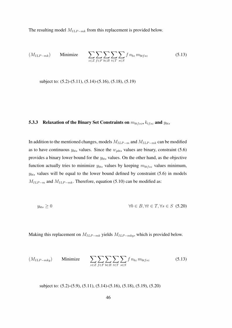
The resulting model MILP−mk from this replacement is provided below.

(MILP−mk) Minimize∑z∈Z

∑f∈F

∑b∈B

∑t∈T

∑s∈S

f nbzmbtfsz (5.13)

subject to: (5.2)-(5.11), (5.14)-(5.16), (5.18), (5.19)

5.3.3 Relaxation of the Binary Set Constraints on mbtfsz, ktfsz and ybts

In addition to the mentioned changes, modelsMILP−m andMILP−mk can be modified

as to have continuous ybts values. Since the wpbts values are binary, constraint (5.6)

provides a binary lower bound for the ybts values. On the other hand, as the objective

function actually tries to minimize ybts values by keeping mbtfsz values minimum,

ybts values will be equal to the lower bound defined by constraint (5.6) in models

MILP−m and MILP−mk. Therefore, equation (5.10) can be modified as:

ybts ≥ 0 ∀b ∈ B, ∀t ∈ T,∀s ∈ S (5.20)

Making this replacement on MILP−mk yields MILP−mky, which is provided below.

(MILP−mky) Minimize∑z∈Z

∑f∈F

∑b∈B

∑t∈T

∑s∈S

f nbzmbtfsz (5.13)

subject to: (5.2)-(5.9), (5.11), (5.14)-(5.16), (5.18), (5.19), (5.20)

46

5.3.4 Relaxation of the Binary Set Constraints on wpbts and mbtfsz

Binary set constraints on variable wpbts in models MILP and MILP−m (i.e., where

xpbts, ybts and ktfsz variables are still binary) can be relaxed without violating the bi-

nary restrictions. Constraint (5.6) provides upper integer bounds for the wpbts values.

However, wpbts values do not have a lower limit aside from constraint (5.5), which

necessitates the sum of wpbts over s ∈ S, t ∈ T . However, as in the case of relaxing

ktfsz variables, there’s no advantage of assigning fractional values for wpbts variables.

If a wpbts is assigned a fractional value, there must be at least one other wpbts > 0 to

satisfy constraint (5.5). If that is the case, constraint (5.4) will require more ybts and

xbts variables to have a value of 1, which would increase the objective value. There-

fore, constraint (5.11) in models MILP and MILP−m can be replaced by (5.21) while

still preserving the binary structure of the solution.

wpbts ≥ 0 ∀p ∈ P, ∀b ∈ B, ∀t ∈ T,∀s ∈ S (5.21)

Resulting models from the mentioned replacements, MILP−m and MILP−mw can be

seen below.

(MILP−w) Minimize∑z∈Z

∑f∈F

∑b∈B

∑t∈T

∑s∈S

f nbzmbtfsz (5.13)

subject to: (5.2)-(5.10), (5.12), (5.14)-(5.17), (5.21)

(MILP−mw) Minimize∑z∈Z

∑f∈F

∑b∈B

∑t∈T

∑s∈S

f nbzmbtfsz (5.13)

subject to: (5.2)-(5.10), (5.12), (5.14)-(5.16), (5.18), (5.21)

47

5.3.5 Relaxation of the Binary Set Constraints on mbtfsz, ktfsz, ybts and wpbts

In addition to the previous models, we also consider relaxing the set constraints on de-

cision variables mbtfsz, ktfsz, ybts and wpbts together. Unlike the previous relaxation,

this one does not guarantee a binary solution, i.e., may yield a fractional solution.

We analyze the structure of the solutions of this model and the time required to solve

it to see if it could be useful in a potential rounding heuristic. The resulting model

MILP−mkwy is provided below.

(MILP−mkwy) Minimize∑z∈Z

∑f∈F

∑b∈B

∑t∈T

∑s∈S

f nbzmbtfsz (5.13)

subject to: (5.2)-(5.9), (5.14)-(5.16), (5.18), (5.19), (5.20), (5.21)

48

CHAPTER 6

COMPUTATIONAL EXPERIMENTS

This chapter of the study introduces the experimental studies for solving the model

presented in Chapter 5. After an introduction to the used problem instances, their

sources and the experiment setup in Section 6.1, the discussion on the results and

validation of the model are presented.

All computational experiments reported in this study were executed on a set of iden-

tical computers with Intel Core i7-4770S 3.1 GHz four-core CPUs and 2x8GB RAM.

All methods used in the experiments were coded on C++, compiled on Microsoft Vi-

sual Studio 2017 15.5.5, and CPLEX software (version 12.9) was called by using the

Concert library.

6.1 Problem Settings and Generation of the Problem Instances

Used problem instances in the computational experiments are small sets sampled from

the analyzed environment’s (AE) ERP database. The algorithm used in the generation

of these small samples can be seen in Appendix E, Algorithm 3. With all the pick

orders and their component lists on hand, this algorithm creates a small problem

instance according to the given parameters. In this study, a problem setting is referred

to a set of parameters for the target data sample, where a problem instance refers to

the unique problem sets generated by using a previously determined setting. Table

6.1 shows the parameters of a setting and the values used in data generation phase of

this study. Each combination of the decisions in Table 6.1 indicates a setting and 10

instances were generated for each of them.

49

Table 6.1: Levels for the parameters defining the problem setting.

Number of Orders (b) Order Size Limits (p) Number of VLM Units (s) Tray Capacities (c)

5, 10, 15 [4, 8], [12, 16], [20, 24] 2, 3, 4 Low, Medium, High

A setting is defined by the following parameters of the problem:

• Number of pick orders,

• Upper and lower size limits for the pick orders, in terms of the number of

requested unique part types,

• The number of VLM machines in the VLM pod,

• Capacities of the trays in terms of the number of different part types.

The size limits for the pick orders make Algorithm 3 only include the orders with a

size within the limits. Therefore, total number of the parts in an instance depends

on the random selection of pick orders. Moreover, Algorithm 3 determines the mini-

mum number of trays according to the tray capacities and the number of parts in the

instance. According to the number of parts in an instance, Algorithm 3 always assigns

the minimum feasible number of trays. Therefore, there is no infeasible problem in-

stance in our experimental study.

Although the current VLM pod in the AE had a fixed VLM pod configuration, the

experiments also consider different VLM configuration and environment settings by

changing the number of VLMs and tray capacities. Outcomes from the experiments

with different settings will be beneficial in understanding the effect of VLM pod

design on the solution procedures and the objective values of the obtained solutions.

Algorithm 3 starts the generation of a problem instance by taking these arguments: the

pool of all pick orders, the number of orders, d, upper and lower limits for the number

of components in the picked orders. Until the number of orders in the considered

setting, d, is reached, the algorithm continues to pick orders with a size within the

given limits. After there are d different orders in the picked list, parts in all the orders

are combined in a unique list. The size of this list determines the number of parts

50

defined in this problem instance, p. There is a one last check before considering this

list of orders as a problem instance input. If there is not even one part that is used

by more than one order, this order list is rejected since it is not likely for the AE to

have all orders having disjoint sets of parts. Lastly, after obtaining the set of parts

and the set of orders, these part and order sets are used to generate different VLM

pod configuration settings. Therefore, one iteration of Algorithm 3 yields 9 different

problem instances with the same parts and orders, but different number of VLMs and

tray capacities. Note that the number of VLMs can be 2, 3 or 4 and tray capacities

can be low, medium or high.

As shown in Table 6.1, each setting has a set of parameters: b, p, s and c. Accord-

ing to the number of decision variables and the number of constraints in the related

models, settings with the lowest number of b, p, s and "High" tray capacity c values

represent the models with smallest size, and hence they are expected to be solved

faster. Therefore, all the experiments in this chapter start with the setting where

b = 5, p = [4, 8], s = 2, c ="High". If a solution method fails to prove optimality in

a time limit of 3 hours for a problem instance, we consider that problem instance as

one that cannot be solved optimally with the selected method. It does not necessarily

mean that our solver, CPLEX, was not able to find a feasible solution. If a problem

setting has 3 or more instances that cannot be solved to optimality in the time limit,

we do not consider solving the instances of any problem setting that is expected to

be more difficult based on the parameters defining the size and the difficulty of the

instance (i.e., parameters presented in Table 6.1).

Since Algorithm 3 only includes the demanded parts in a problem instance, models

presented in Chapter 5 can be modified slightly. In the proposed models, constraint

(5.2) forces the parts to be assigned to at least one storage location. However, if a part

is requested in an order, constraints (5.4) and (5.5) already force the model to assign

a storage location for that part. Therefore, constraint (5.2) can be removed if all the

parts stored in the VLM unit are requested by at least one order in the planned period.

All the model alternatives were ran with and without the constraint (5.2), and a slight

improvement in solution times were seen. Therefore, this section only reports the

experiment results on the models without constraint (5.2).

51

In any case where unused parts need to be stored in a VLM, the decision maker can

exclude the unused parts from the model’s input. Then, those parts can be assigned

to the remaining empty locations after obtaining the solution. Since unused parts will

have no contribution to the objective function value, this approach (i.e., solving the

model without constraint (5.2)) will still yield the same objective function value.

6.2 Computational Performance for the Proposed Models

Since version 12.5.1, CPLEX uses the proposition by Li (1994) to convert models

with linear constraints, non-linear objective functions to linear models (Puget, 2013).

Therefore, MQP is not included in the experiments, since it will already be converted

to model MILP by CPLEX in the preprocessing phase.

The experiments described in this section start by attempting to solve the instances in

the easiest problem setting having the least number of decision variables. This setting

is shown on the top-left corner of Table 6.2 (i.e., b = 5, p = [4, 8], s = 2, c ="High").

In the next steps, if 3 or more instances out of 10 cannot be solved to optimality

within the allowed time limit for a setting, we did not consider the settings which

are computationally more challenging. For this problem, increasing one of the b, p,

or s values; or lowering the tray capacity c, while keeping the other 3 parameters

unchanged, is considered to make a setting more complex, mainly due to the number

of constraints and decision variables.

Experiments involving model MILP were able to reach optimality for 162 problem

instances out of 810. The number of solved instances (nS) for each problem setting

can be seen in Table 6.2. In this table, highlighted cells indicate the settings with 3 or

more unsolved instances. The cells with a "-" value indicate the settings that are more

complex than any of the settings with 3 or more unsolved instances, and hence not

considered. According to the reported values of solved instances, having a high tray

capacity, i.e., closer to the average order size, makes the problem easier to solve. On

the other hand, increased number of orders, increased number of parts and increased

number of VLM units in a problem make the problem more difficult, so we observe

degrading computational performance in those directions.

52

Table 6.2: Number of solved instances (nS) out of 10 instances for each setting, using

model MILP .

MILP , nSs = 2 s = 3 s = 4

c =High c =Mid c =Low c =High c =Mid c =Low c =High c =Mid c =Low

b=

5 p ∈ [4, 8] 10 10 7 10 10 - 10 4 -

p ∈ [12, 16] 10 0 - 10 - - 10 - -

p ∈ [20, 24] 10 - - 10 - - 9 - -

b=

10

p ∈ [4, 8] 10 0 - 10 - - 3 - -

p ∈ [12, 16] 1 - - - - - - - -

p ∈ [20, 24] - - - - - - - - -

b=

15

p ∈ [4, 8] 10 - - 8 - - - - -

p ∈ [12, 16] - - - - - - - - -

p ∈ [20, 24] - - - - - - - - -

Since CPLEX cannot find the solutions using model MILP for most of the instances

in our experiments, we tested the performance of modified versions of our model

described in Section 5.3. This part of the study discusses those modifications (i.e.,

relaxation alternatives) and their performance as in terms of the number of solved

instances for all settings and solution times. Please note that solvingMILP−mkwy may

not yield an optimal solution due to the relaxation of wpbts variables, as discussed in

Section 5.3.5.

The number of problem instances solved to optimality can be seen in Table 6.3. Ac-

cording to those numbers, using modelMILP−mk performs best. Detailed information

about the number of solved instances for each setting and each model can be seen in

Table 6.4. Please note that the solutions obtained using model MILP−mkwy are differ-

ent from the rest of the models presented since it allows fractional decision variables.

Table 6.3: Number of solved instances out of 810 for each model.

Model Number of solved instances (nS)

MILP 162

MILP−m 173

MILP−mk 193

MILP−mky 173

MILP−w 134

MILP−mw 156

MILP−mkwy 39

53

When looking at Tables 6.2 and 6.4, some changes in the model’s limits can be no-

ticed between each model. For example, relaxing the set constraints on the lineariza-

tion variable, mbtfsz, causes a very small change in the number of solved instances.

On the other hand, relaxing the set constraints on the ktfsz variables increase the solv-

ability particularly for the settings on the far right side on Table 6.4, where the total

number of trays and VLM units become higher. This improvement is not surprising,

considering the fact that ktfsz variables represent the assignment decisions of trays to

shelves in VLM units.

Solution time (in CPU seconds), number of unsolved instances (nUS) and the corre-

sponding optimality gap values for each setting are reported in Tables 6.5-6.6. Each

row in these tables represents a setting (defined by their p, b, c and s values), and the

average and maximum values are reported across the instances in that setting. Ag-

gregate measures, i.e., average and maximum, for solution time are calculated over

the instances that can be solved in that problem setting. On the other hand, aggregate

measures for the optimality gaps are calculated over the unsolved instances of the

corresponding setting and presented as percentages in columns titled %Gap. Table

cells with N/A values represent the problem settings that are not considered since the

corresponding model fails to solve more than 3 instances of easier problem instances.

The results show that some of the relaxation alternatives, such as MILP−mk provide

improvements in solution times, thus the maximum problem size that can be solved

in the time limits. According to the results, it is clear that having trays with higher

capacities makes the problem easier to solve.

In these computational experiments consisting of using 7 different models, we iden-

tified some benefits in the solution times after relaxing the binary set constraints for

some sets of decision variables. On the other hand, these models also showed that

a real life scenario consisting of more parts than our experimental settings may re-

quire a high-end computing environment, or a different solution method that may

make some sacrifices in terms of the solution quality, in order to get a solution in a

reasonable amount of time. Model MILP−mkwy was developed with that option in

consideration: getting a non-integer solution and then obtaining a feasible solution

by using rounding heuristics. In fact, models MILP−mkwy and MILP−mkwy−red yield

54

solutions with fractional values for decision variables and can be used in rounding

procedures. However, the solution times for these models were higher than the other

model alternatives. Upon an investigation of the solution procedure, we detected that

our solver, CPLEX, evaluates a much higher number of nodes during its search for

the optimal solution, which makes using this model to obtain solutions to be rounded

impractical.

55

Table 6.4: Number of solved instances out of 10 by using modelsMILP−m,MILP−mk,

MILP−mky.

MILP−ms = 2 s = 3 s = 4


b=

5 p ∈ [4, 8] 10 10 8 10 10 9 10 3 -

p ∈ [12, 16] 10 0 - 10 - - 10 - -

p ∈ [20, 24] 10 - - 10 - - 9 - -

b=

10

p ∈ [4, 8] 10 0 - 10 - - 5 - -

p ∈ [12, 16] 1 - - - - - - - -

p ∈ [20, 24] - - - - - - - - -

b=

15

p ∈ [4, 8] 10 - - 8 - - - - -

p ∈ [12, 16] - - - - - - - - -

p ∈ [20, 24] - - - - - - - - -

MILP−mks = 2 s = 3 s = 4


b=

5 p ∈ [4, 8] 10 10 10 10 10 10 10 10 10

p ∈ [12, 16] 10 0 - 10 - - 10 - -

p ∈ [20, 24] 10 - - 10 - - 10 - -

b=

10

p ∈ [4, 8] 10 0 - 10 - - 5 - -

p ∈ [12, 16] 2 - - - - - - - -

p ∈ [20, 24] - - - - - - - - -

b=

15

p ∈ [4, 8] 9 - - 7 - - - - -

p ∈ [12, 16] - - - - - - - -

p ∈ [20, 24] - - - - - - - - -

MILP−mkys = 2 s = 3 s = 4


b=

5 p ∈ [4, 8] 10 10 10 10 10 8 10 9 8

p ∈ [12, 16] 10 0 - 10 - - 8 - -

p ∈ [20, 24] 10 - - 10 - - 9 - -

b=

10

p ∈ [4, 8] 10 0 - 10 - - 2 - -

p ∈ [12, 16] 0 - - - - - - - -

p ∈ [20, 24] - - - - - - - - -

b=

15

p ∈ [4, 8] 8 - - 1 - - - - -

p ∈ [12, 16] - - - - - - - - -

p ∈ [20, 24] - - - - - - - - -

continued...

56

Table 6.4: Number of solved instances out of 10 by using modelsMILP−m,MILP−mk,

MILP−mky.

MILP−ws = 2 s = 3 s = 4


b=

5 p ∈ [4, 8] 10 10 4 10 10 - 10 1 -

p ∈ [12, 16] 10 0 - 10 - - 10 - -

p ∈ [20, 24] 10 - - 10 - - 9 - -

b=

10

p ∈ [4, 8] 10 0 - 10 - - - - -

p ∈ [12, 16] 0 - - - - - - - -

p ∈ [20, 24] - - - - - - - - -

b=

15

p ∈ [4, 8] - - - - - - - - -

p ∈ [12, 16] - - - - - - - - -

p ∈ [20, 24] - - - - - - - - -

MILP−mws = 2 s = 3 s = 4


b=

5 p ∈ [4, 8] 10 10 4 10 10 - 10 1 -

p ∈ [12, 16] 10 0 - 10 - - 10 - -

p ∈ [20, 24] 10 - - 10 - - 9 - -

b=

10

p ∈ [4, 8] 10 0 - 10 - - 4 - -

p ∈ [12, 16] 0 - - - - - - - -

p ∈ [20, 24] - - - - - - - - -

b=

15

p ∈ [4, 8] 10 - - 8 - - - - -

p ∈ [12, 16] - - - - - - - - -

p ∈ [20, 24] - - - - - - - - -

MILP−mkwys = 2 s = 3 s = 4


b=

5 p ∈ [4, 8] 10 5 - 6 - - - - -

p ∈ [12, 16] 9 0 - - - - - - -

p ∈ [20, 24] 4 - - - - - - - -

b=

10

p ∈ [4, 8] 5 - - - - - - - -

p ∈ [12, 16] - - - - - - - - -

p ∈ [20, 24] - - - - - - - - -

b=

15

p ∈ [4, 8] - - - - - - - - -

p ∈ [12, 16] - - - - - - - - -

p ∈ [20, 24] - - - - - - - - -

57

Tabl

e6.

5:So

lutio

ntim

ean

dop

timal

ityga

pva

lues

form

odel

sM

ILP

,MILP−m

,MILP−mk,M

ILP−mky;i

nea

chpr

oble

mse

tting

.

pb

cs

MILP

MILP−m

MILP−mk

MILP−mky

nUS

CPU

Tim

e(s

ec.)

%Gap

nUS

CPU

Tim

e(s

ec.)

%Gap

nUS

CPU

Tim

e(s

ec.)

%Gap

nUS

CPU

Tim

e(s

ec.)

%Gap

avg.

max

.av

g.m

ax.

avg.

max

.av

g.m

ax.

avg.

max

.av

g.m

ax.

avg.

max

.av

g.m

ax.

4-8

5H

igh

2-

0.26

0.58

--

-0.

180.

23-

--

0.26

0.38

--

-0.

501.

27-

-

4-8

5H

igh

3-

1.83

8.00

--

-1.

706.

57-

--

2.00

6.18

--

-4.

3513

.01

--

4-8

5H

igh

4-

231.

8215

23.3

7-

--

131.

5165

4.04

--

-22

.61

49.7

3-

--

62.6

911

4.73

--

4-8

5M

id2

-12

1.51

566.

43-

--

120.

1456

3.31

--

-12

.13

20.7

6-

--

55.4

416

8.55

--

4-8

5M

id3

-12

30.7

742

11.9

1-

--

1190

.75

4007

.42

--

-46

.75

180.

27-

--

339.

7210

41.0

0-

-

4-8

5M

id4

662

03.2

310

731.

5011

147

4764

.31

8240

.03

915

-73

3.74

2523

.49

--

124

92.3

574

08.0

422

22

4-8

5L

ow2

349

8.96

861.

516

122

515.

2883

6.99

33

-11

0.80

281.

31-

--

1045

.17

5401

.23

--

4-8

5L

ow3

N/A

N/A

N/A

N/A

N/A

121

39.2

190

75.8

012

12-

1079

.49

9279

.95

--

267

4.26

1869

.22

1619

4-8

5L

ow4

N/A

N/A

N/A

N/A

N/A

N/A

N/A

N/A

N/A

N/A

-64

1.69

4867

.10

--

212

19.6

230

90.0

011

13

4-8

10H

igh

2-

2.89

8.10

--

-2.

928.

63-

--

15.8

532

.33

--

-25

.97

116.

58-

-

4-8

10H

igh

3-

192.

0348

4.11

--

-18

7.27

482.

01-

--

266.

0167

6.30

--

-84

8.95

2105

.72

--

4-8

10H

igh

47

3603

.61

5435

.02

510

564

46.2

210

123.

106

105

2941

.92

4567

.48

713

832

87.5

250

80.5

811

18

4-8

10M

id2

10-

-56

7110

--

5871

10-

-44

5310

--

6168

4-8

15H

igh

2-

124.

5010

71.0

6-

--

141.

3512

42.9

4-

-1

1132

.65

3698

.70

1010

239

5.23

859.

5739

44

4-8

15H

igh

32

841.

9357

20.3

44

42

841.

2057

14.6

94

43

4788

.64

7030

.07

1314

926

90.6

626

90.6

69

18

12-1

65

Hig

h2

-0.

841.

21-

--

0.87

1.47

--

-1.

382.

58-

--

6.13

10.1

3-

-

12-1

65

Hig

h3

-19

.00

38.2

8-

--

19.4

737

.30

--

-17

.61

47.5

5-

--

143.

5726

3.54

--

12-1

65

Hig

h4

-14

0.41

247.

84-

--

140.

0524

0.33

--

-17

6.24

342.

43-

-2

1783

.51

6548

.97

68

12-1

65

Mid

210

--

4159

10-

-45

6910

--

2940

10-

-56

67

12-1

610

Hig

h2

998

90.1

398

90.1

316

339

1014

9.70

1014

9.70

1633

866

35.1

076

31.0

814

2410

--

4464

12-1

615

Hig

h2

N/A

N/A

N/A

N/A

N/A

N/A

N/A

N/A

N/A

N/A

10-

-62

82N

/AN

/AN

/AN

/AN

/A

20-2

45

Hig

h2

-15

6.97

402.

63-

--

159.

6240

3.89

--

-17

.33

32.7

5-

--

169.

3384

3.26

--

20-2

45

Hig

h3

-29

.33

41.5

9-

--

29.8

643

.12

--

-23

.90

32.1

0-

--

330.

8413

92.7

9-

-

20-2

45

Hig

h4

169

6.25

3954

.05

55

112

11.9

786

00.0

24

4-

444.

7410

30.5

6-

-1

3435

.05

7179

.06

22

58

Tabl

e6.

6:So

lutio

ntim

ean

dop

timal

ityga

pva

lues

form

odel

sM

ILP−w

,MILP−mw

,MILP−mkwy;i

nea

chpr

oble

mse

tting

.

pb

cs

MILP−w

MILP−mw

MILP−mkwy

nUS

CPU

Tim

e(s

ec.)

%Gap

nUS

CPU

Tim

e(s

ec.)

%Gap

nUS

CPU

Tim

e(s

ec.)

%Gap

avg.

max

.av

g.m

ax.

avg.

max

.av

g.m

ax.

avg.

max

.av

g.m

ax.

4-8

5H

igh

2-

0.18

0.31

--

-0.

180.

26-

--

24.1

283

.34

--

4-8

5H

igh

3-

1.16

5.86

--

-0.

721.

48-

-4

1882

.60

7133

.36

3944

4-8

5H

igh

4-

112.

3439

7.27

--

-11

1.41

392.

38-

-N

/AN

/AN

/AN

/AN

/A

4-8

5M

id2

-98

.03

358.

52-

--

102.

2935

8.80

--

538

2.51

1728

.15

6598

4-8

5M

id3

-10

65.2

835

10.9

7-

--

917.

1233

44.4

8-

-N

/AN

/AN

/AN

/AN

/A

4-8

5M

id4

947

47.5

547

47.5

510

189

5048

.87

5048

.87

1018

N/A

N/A

N/A

N/A

N/A

4-8

5L

ow2

641

8.60

933.

0216

296

415.

7194

4.80

1529

N/A

N/A

N/A

N/A

N/A

4-8

5L

ow3

N/A

N/A

N/A

N/A

N/A

N/A

N/A

N/A

N/A

N/A

N/A

N/A

N/A

N/A

N/A

4-8

5L

ow4

N/A

N/A

N/A

N/A

N/A

N/A

N/A

N/A

N/A

N/A

N/A

N/A

N/A

N/A

N/A

4-8

10H

igh

2-

3.51

12.0

7-

--

3.72

12.7

0-

-5

2583

.09

8907

.45

3349

4-8

10H

igh

3-

296.

3382

1.84

--

-27

0.81

767.

65-

-N

/AN

/AN

/AN

/AN

/A

4-8

10H

igh

4N

/AN

/AN

/AN

/AN

/A6

5242

.71

8593

.28

57

N/A

N/A

N/A

N/A

N/A

4-8

10M

id2

10-

-41

7010

--

3945

N/A

N/A

N/A

N/A

N/A

4-8

15H

igh

2N

/AN

/AN

/AN

/AN

/A-

191.

8816

30.4

9-

-N

/AN

/AN

/AN

/AN

/A

4-8

15H

igh

3N

/AN

/AN

/AN

/AN

/A2

1286

.76

8652

.17

33

N/A

N/A

N/A

N/A

N/A

12-1

65

Hig

h2

-1.

182.

02-

--

1.12

1.92

--

112

54.2

643

85.3

25

5

12-1

65

Hig

h3

-29

.93

52.3

5-

--

28.6

152

.36

--

N/A

N/A

N/A

N/A

N/A

12-1

65

Hig

h4

-37

4.47

1896

.84

--

-37

4.48

1900

.70

--

N/A

N/A

N/A

N/A

N/A

12-1

65

Mid

210

--

5579

10-

-55

7910

--

100

100

12-1

610

Hig

h2

10-

-16

3210

--

1632

N/A

N/A

N/A

N/A

N/A

12-1

615

Hig

h2

N/A

N/A

N/A

N/A

N/A

N/A

N/A

N/A

N/A

N/A

N/A

N/A

N/A

N/A

N/A

20-2

45

Hig

h2

-14

6.42

304.

66-

--

144.

4630

1.56

--

624

96.8

798

15.4

287

100

20-2

45

Hig

h3

-66

.26

165.

66-

--

65.4

316

5.35

--

N/A

N/A

N/A

N/A

N/A

20-2

45

Hig

h4

194

4.32

3522

.30

99

193

6.22

3525

.51

99

N/A

N/A

N/A

N/A

N/A

59

6.3 Quality of the Obtained Solutions

Based on our observations from the real-life system, AE’s transaction history and

the analyses regarding the throughput related VLM pod decisions; we propose stor-

age assignments based on model MILP to increase throughput in VLM pods. MILP

tries to increase throughput by reducing the time spent for tray retrievals through the

use of an objective function of minimizing total weighted number of tray retrievals,

where trays in higher shelves have higher weight values. This section discusses the

performance of the obtained solutions in terms of the increase achieved in system

throughput in VLM pods. Discussion in this section is based on the 196 instances

that were solved to optimality in the experiments in Section 6.2. The distribution of

the solved instances over problem settings can be seen in Table 6.7. Average of the

optimal objective values for each problem setting can be seen in Table 6.8.

Values in Table 6.8 show that having smaller trays, thus, a higher number of trays

in the VLM pod in such small instances hurts the objective function. This is not

unexpected, because the objective function of the model is based on the number of

tray retrievals. The optimal value also increases with an increase in the number of

parts. Since the generated problem instances have bigger tray sizes (and hence lower

number of trays) as the number of parts increase, the change in the objective function

is less steep than the increase in the case with a higher number of trays.

Table 6.7: Number of obtained optimal values from the overall experimental runs for

all used problem instances.

s = 2 s = 3 s = 4


b=

5 p ∈ [4, 8] 10 10 10 10 10 10 10 10 10

p ∈ [12, 16] 10 0 0 10 0 0 10 0 0

p ∈ [20, 24] 10 0 0 10 0 0 10 0 0

b=

10

p ∈ [4, 8] 10 0 0 10 0 0 6 0 0

p ∈ [12, 16] 2 0 0 0 0 0 0 0 0

p ∈ [20, 24] 0 0 0 0 0 0 0 0 0

b=

15

p ∈ [4, 8] 10 0 0 8 0 0 0 0 0

p ∈ [12, 16] 0 0 0 0 0 0 0 0 0

p ∈ [20, 24] 0 0 0 0 0 0 0 0 0

60

Table 6.8: Average optimal values obtained from all experimental runs.

avg. opt. val.s = 2 s = 3 s = 4

c =High c =Mid c =Low c =High c =Mid c =Low c =High c =Mid c =Lowb

=5 p ∈ [4, 8] 144.1 358.5 600.9 170.3 284.7 457.1 213.3 342.3 389.4

p ∈ [12, 16] 182.1 - - 223.8 - - 262.3 - -

p ∈ [20, 24] 270.1 - - 227.2 - - 252.2 - -

b=

10

p ∈ [4, 8] 254.1 - - 274.2 - - 298.3 - -

p ∈ [12, 16] 424.5 - - - - - - - -

p ∈ [20, 24] - - - - - - - - -

b=

15

p ∈ [4, 8] 389.2 - - 377.6 - - - - -

p ∈ [12, 16] - - - - - - - - -

p ∈ [20, 24] - - - - - - - - -

In order to verify the proposed model’s benefits on a VLM pod’s throughput, the op-

timal solutions obtained in Section 6.2 were used in a picking simulation (simulation

model is described in Appendix C). These picking simulations also consider the cur-

rent storage assignment decisions used in the AE’s VLM pod. This section presents

comparison of the current system with the proposed one. Considered decisions and

their alternative set of actions in this simulation are as follows:

Location Assignment Rules: In addition to the optimal solution for MILP , two

other storage assignment rules are simulated. AE purchases all components for a

customer order project in bulk and accepts them together at the warehouse. Therefore,

each project’s component parts are typically stored closer to each other at first location

assignments. This grouping is similar to the pick order based grouping done byMILP ,

but with a low level of detail since there are less than 10 projects, but more than

12,000 different pick order types at the AE. However, as part locations are not fixed,

closest open location assignments for the replenishments cause AE to reach random

storage assignment in the long run (see Section 2.2.3 and Figure A.10 in Appendix

A). Therefore, the current storage assignment scheme’s performance is assumed to be

between that of project based grouping and random assignment.

VLM Unit Sequencing: The orders consisting parts from more than one VLM unit

in the pod are making the operator walk between VLM units. As discussed in Chapter

61

3, there are two alternative decisions for the operator after completing all the picks

from a tray. The operator may wait for the next tray (will be referred as "wait") or go

to the other VLM unit on which the tray may be ready (will be referred as "walk").

Results from the preliminary VLM pod picking simulation described in Appendix C

already show that walking to the other VLM unit during tray retrievals is the better

choice for both of the random storage and turnover based location assignment cases.

Table 6.9: Simulated scenarios in the verification phase.

Scenario

No.

Walk Duration Between Units

(seconds)

Number of

VLMs

Location

Assignments

VLM Unit

Sequencing Rule

1 7 2 MILP Walk

2 7 2 MILP Wait

3 7 2 Random Walk

4* 7 2 Random Wait

5 7 2 Project groups Walk

6* 7 2 Project groups Wait

This simulation considers 6 different scenarios for each of the problem instances

which are summarized in Table 6.9. In the table, * indicates the scenarios reflecting

the current real life situation at the AE. Performance measure values of the real-life

system in AE is assumed to be between the performance measure values of scenar-

ios 4 and 6. For each problem instance, 30 replications were run. The simulation

steps can be seen in Algorithm 4 in Appendix E. Completion time of the last pick

order (cmax), average operator utilization and number of tray retrievals are among the

recorded performance measures.

Assumptions of the Simulation: This simulation assumes the following:

• All the VLM units in the VLM pod are identical.

• All trays have the same box layout and all trays have c boxes, where c is deter-

mined by the parameters of the simulated problem instance.

• Different part types cannot be stored in the same box.

• Boxes are large enough to accommodate any number of stored parts.

62

• After an order’s picks are completed, the last tray stays on the I/O point of

the VLM unit. In other words, dual cycle tray retrievals are used in between

different orders.

• Each order’s pick process starts from the closest tray to the I/O point.

• Task times follow normal distribution with the parameters found in time study

presented in Section 2.3.2.

• There are enough on hand stock for all parts ordered during each replication.

Therefore, there are no stock replenishment operations in the simulated period.

• Only pick tasks arrive into the system. Put and count operations are assumed

to be carried on during periods that are not considered in this simulation.

• Operator works at a constant pace.

Observations: In this part, Scenario 1 is considered as our suggested system, whereas

the current system is assumed to be between Scenario 4 and Scenario 6. Performance

measures of these three scenarios are given in Tables 6.16-6.19, where a detailed list

of the performance measures for all scenarios can be seen in Appendix E, Tables

E.2 and E.3. All presented values in these tables are averages across 30 simulation

replications for 10 problem instances of the indicated problem setting.

The average number of tray retrievals in Table 6.19 shows thatMILP performs well in

terms of minimizing the number of tray retrievals in the system. Since the objective

function of MILP is based on the number of tray retrievals, this is expected. Average

values of the number of tray retrievals in each scenario and setting are given in Table

6.19, where the average percentage improvement of the number of tray retrievals in

Scenario 1, in comparison with Scenario 6 or Scenario 4, can be seen in Tables 6.10

and 6.11. In this table, improvement ratios of Scenario 6 and Scenario 4 are on the

same cells, separated with a "-" in between. In overall, Scenario 1, Scenario 4 and

Scenario 6 yielded the average number of tray retrievals as 125.8, 444.7 and 341.8,

respectively. The improvements in the number of tray retrievals in Scenario 1 increase

as the number of parts in the problem setting increase. Since scenarios 4 and 6 include

random storage, they are expected to perform better in settings with less number of

63

parts since the probability of having two parts on the same tray increases when the

number of parts to locate decreases. On the other hand, as tray sizes get smaller (i.e.,

movement from the left hand side of Table 6.10 to the right), improvements obtained

in Scenario 1 decreases. This shows that as tray sizes get smaller than the average

order size, advantages of using MILP may decrease.

Table 6.10: % improvements in the number of tray retrievals in Scenario 1, compared

with Scenario 4.

%∆Num.Tray Ret. s = 2 s = 3 s = 4

Scenario 1 vs. 4 c =High c =Mid c =Low c =High c =Mid c =Low c =High c =Mid c =Low

b=

5 p ∈ [4, 8] 72.4 54.5 42.4 67.2 57.8 43.7 65.3 60.2 44.9

p ∈ [12, 16] 76.5 - - 81.8 - - 78.1 - -

p ∈ [20, 24] 75.3 - - 83.5 - - 82.5 - -

b=

10

p ∈ [4, 8] 82.1 - - 78.2 - - 76.1 - -

p ∈ [12, 16] 83.2 - - - - - - - -

p ∈ [20, 24] - - - - - - - - -

b=

15

p ∈ [4, 8] 80.4 - - 81.0 - - - - -

p ∈ [12, 16] - - - - - - - - -

p ∈ [20, 24] - - - - - - - - -

Table 6.11: % improvements in the number of tray retrievals in Scenario 1, compared

with Scenario 6.

%∆Num.Tray Ret. s = 2 s = 3 s = 4


b=

5 p ∈ [4, 8] 67.5 46.6 36.8 56.7 47.9 35.9 57.5 46.9 39.2

p ∈ [12, 16] 71.1 - - 74.8 - - 64.7 - -

p ∈ [20, 24] 66.4 - - 75.5 - - 71.2 - -

b=

10

p ∈ [4, 8] 77.9 - - 73.5 - - 70.2 - -

p ∈ [12, 16] 78.5 - - - - - - - -

p ∈ [20, 24] - - - - - - - - -

b=

15

p ∈ [4, 8] 74.4 - - 75.5 - - - - -

p ∈ [12, 16] - - - - - - - - -

p ∈ [20, 24] - - - - - - - - -

64

When the results of this simulation are compared with the results from the picking

simulation of the real-life VLM system (see Appendix C for the mentioned simula-

tion), we notice that the operator utilization ratios are higher in the simulation of the

small problem instances in each scenario. These high utilization ratios may also be

an indicator of a bottleneck situation in the VLM pod. The operator’s utilization in-

cludes the time spent for pick tasks and walks. On the other hand, a picking operation

in a VLM pod consists of the operator’s manual picks from the tray, tray retrievals in

VLM units, and the occasional walks and waits. As stated in Section 2.3.2 and Ap-

pendix D, tray retrieval times depend on the height of the VLM unit. Since the small

settings generated for the experimental study have small sets of parts, the total num-

ber of trays is also less than the real-life case in these reduced problem instances. The

average number of trays per VLM unit among all of 196 solved problem instances is

2.6, which is extremely low compared to 114 trays per VLM in the real-life setup at

the AE. Since a tray retrieval cycle’s duration is dependent on the vertical distance

traveled, problem settings with less number of trays will have faster tray retrievals. In

such a case, the operator is more likely to act as the bottleneck of the system, and the

picking cycle will be more likely to reflect the operator task times. As discussed in

Chapter 3, if a VLM system has a highly utilized operator, making VLM tray retrieval

times shorter should not be the priority of the decision-maker; therefore, MILP is less

relevant in that case.

When the cmax values for Scenario 1 and Scenarios 6 and 4 are compared, the issue of

high operator utilization levels should be considered, too. As seen in Table 6.17, there

are some problem settings with operator utilization levels of more than 95%. Since

MILP aims to reduce tray retrieval times, thus, also walks and waits caused by tray

retrievals; the objective function of MILP may not reflect the situation well enough

when the operator is the system’s bottleneck. This does not mean that applying MILP

will hurt the system’s performance. It only means that the gains in the performance

in terms of system throughput may not be high enough in such a case. The average

cmax values for each problem setting and each of the considered scenarios in Table

6.16 also indicate this issue. Although there is no case where the system in Scenario

1 performs worse than Scenarios 4 and 6, using MILP , i.e., Scenario 1, in some of the

problem settings, such as b = 5, p = 12 − 16, s = 2, c =High, this approach yields

65

smaller improvements since the tray retrievals make up a smaller portion of the system

throughput. Since the small tray counts in these considered settings are not likely to

be encountered, we expect a real-life setup to have higher tray retrieval times. Percent

improvements in the cmax values of Scenario 1 and Scenarios 4 and 6 can be seen in

Tables 6.14 and 6.15. These results show that using MILP leads to improvements

on the cmax values in all settings. As the number of VLM units and the number of

trays increase, i.e., going from left to right in Table 6.14, improvements obtained

from using MILP become higher. Since there are some cases where the operator is

highly utilized, it is not easy to make a comment on the magnitude of average cmax

improvements obtained by using MILP . However, these simulations show that MILP

performs well in terms of reducing the picking times of a VLM system, compared to

the applications at the AE. Since the improvements obtained from MILP in terms of

the number of tray retrievals are between 65% and 70%, we can conclude that MILP

performs well in terms of grouping the parts according to the pick orders.

UsingMILP for the storage assignments yields improvements even in the cases where

the operator was fully utilized. This is expected since the utilization figures also

include the time spent walking. MILP reduces the total walk distances in picking

tours, so a slight improvement may be expected even if the operator is fully utilized.

Time spent walking in each scenario can be seen in Table 6.18, where the percent

improvements of the same metric can be seen in Tables 6.12 and 6.13.

As a final note, although using a VLM unit sequencing rule as "walk" improves the

system throughput, using MILP minimizes that decision’s impact. If all the pick

orders require at most one tray from each VLM unit, two alternative decisions for the

VLM unit sequencing problem will become identical. The difference of cmax values

between Scenario 1 and Scenario 2 is only 30 seconds out of 28,100, which shows

that using MILP makes most of the pick orders require at most one tray from each

VLM unit. This shows that MILP is successful both in grouping the parts of an order

together and distributing trays among the VLM units evenly.

66

Table 6.12: % improvements in the time spent walking in Scenario 1, compared with

Scenario 4.

%∆Walk Time s = 2 s = 3 s = 4


b=

5 p ∈ [4, 8] 69 54 42 61 46 34 48 44 34

p ∈ [12, 16] 74 - - 68 - - 64 - -

p ∈ [20, 24] 78 - - 66 - - 63 - -

b=

10

p ∈ [4, 8] 74 - - 69 - - 66 - -

p ∈ [12, 16] 83 - - - - - - - -

p ∈ [20, 24] - - - - - - - - -

b=

15

p ∈ [4, 8] 78 - - 78 - - - - -

p ∈ [12, 16] - - - - - - - - -

p ∈ [20, 24] - - - - - - - - -

Table 6.13: % improvements in the time spent walking in Scenario 1, compared with

Scenario 6.

∆Walk Time s = 2 s = 3 s = 4


b=

5 p ∈ [4, 8] 61 42 25 49 30 25 38 35 28

p ∈ [12, 16] 64 - - 60 - - 56 - -

p ∈ [20, 24] 61 - - 58 - - 50 - -

b=

10

p ∈ [4, 8] 63 - - 62 - - 61 - -

p ∈ [12, 16] 77 - - - - - - - -

p ∈ [20, 24] - - - - - - - - -

b=

15

p ∈ [4, 8] 69 - - 71 - - - - -

p ∈ [12, 16] - - - - - - - - -

p ∈ [20, 24] - - - - - - - - -

67

Table 6.14: % improvements in the order picking completion times in Scenario 1,

compared with 4.

%∆ cmax s = 2 s = 3 s = 4


b=

5 p ∈ [4, 8] 10.4 11.4 11.3 13.4 13.6 12.3 14.1 14.8 12.5

p ∈ [12, 16] 3.7 - - 8.9 - - 12.2 - -

p ∈ [20, 24] 3.6 - - 6.0 - - 9.1 - -

b=

10

p ∈ [4, 8] 12.6 - - 15.1 - - 15.9 - -

p ∈ [12, 16] 8.3 - - - - - - - -

p ∈ [20, 24] - - - - - - - - -

b=

15

p ∈ [4, 8] 12.8 - - 15.1 - - - - -

p ∈ [12, 16] - - - - - - - - -

p ∈ [20, 24] - - - - - - - - -

Table 6.15: % improvements in the order picking completion times in Scenario 1,

compared with Scenario 6.

%∆ cmax s = 2 s = 3 s = 4


b=

5 p ∈ [4, 8] 10.0 10.3 13.0 11.7 10.9 11.1 11.2 10.0 11.3

p ∈ [12, 16] 4.0 - - 7.0 - - 8.2 - -

p ∈ [20, 24] 4.3 - - 4.0 - - 5.7 - -

b=

10

p ∈ [4, 8] 11.6 - - 12.9 - - 13.3 - -

p ∈ [12, 16] 7.0 - - - - - - - -

p ∈ [20, 24] - - - - - - - - -

b=

15

p ∈ [4, 8] 11.1 - - 12.8 - - - - -

p ∈ [12, 16] - - - - - - - - -

p ∈ [20, 24] - - - - - - - - -

68

Table 6.16: Average order picking completion times (cmax) in the considered scenar-

ios.

Scenario 1 s = 2 s = 3 s = 4

cmax c =High c =Mid c =Low c =High c =Mid c =Low c =High c =Mid c =Low

b=

5 p ∈ [4, 8] 12755.52 13713.88 13778.98 12739.46 13358.76 13474.60 12933.01 16254.24 13579.05

p ∈ [12, 16] 33779.05 - - 31463.11 - - 31550.54 - -

p ∈ [20, 24] 52267.52 - - 52780.49 - - 50978.23 - -

b=

10

p ∈ [4, 8] 25099.71 - - 25102.87 - - 25721.57 - -

p ∈ [12, 16] 60601.06 - - - - - - - -

p ∈ [20, 24] - - - - - - - - -

b=

15

p ∈ [4, 8] 38840.55 - - 39327.90 - - - - -

p ∈ [12, 16] - - - - - - - - -

p ∈ [20, 24] - - - - - - - - -

Scenario 4 s = 2 s = 3 s = 4


b=

5 p ∈ [4, 8] 14231.02 15476.64 15539.17 14715.20 15463.32 15357.63 15058.57 19072.33 15513.70

p ∈ [12, 16] 35065.77 - - 34544.59 - - 35925.78 - -

p ∈ [20, 24] 54206.91 - - 56150.50 - - 56082.23 - -

b=

10

p ∈ [4, 8] 28712.84 - - 29574.50 - - 30569.20 - -

p ∈ [12, 16] 66101.67 - - - - - - - -

p ∈ [20, 24] - - - - - - - - -

b=

15

p ∈ [4, 8] 44557.90 - - 46345.59 - - - - -

p ∈ [12, 16] - - - - - - - - -

p ∈ [20, 24] - - - - - - - - -

Scenario 6 s = 2 s = 3 s = 4


b=

5 p ∈ [4, 8] 14170.62 15262.42 15600.31 14433.05 14922.21 15085.20 14566.10 18045.24 15183.18

p ∈ [12, 16] 35151.92 - - 33840.12 - - 34324.48 - -

p ∈ [20, 24] 54640.20 - - 54976.63 - - 54067.38 - -

b=

10

p ∈ [4, 8] 28407.79 - - 28835.99 - - 29670.80 - -

p ∈ [12, 16] 65149.64 - - - - - - - -

p ∈ [20, 24] - - - - - - - - -

b=

15

p ∈ [4, 8] 43698.06 - - 45111.67 - - - - -

p ∈ [12, 16] - - - - - - - - -

p ∈ [20, 24] - - - - - - - - -

69

Table 6.17: Average operator utilization levels (Op.Util.) in the considered scenarios.

Scenario 1 s = 2 s = 3 s = 4

%Op.Util. c =High c =Mid c =Low c =High c =Mid c =Low c =High c =Mid c =Low

b=

5 p ∈ [4, 8] 95 92 91 97 96 94 99 97 96

p ∈ [12, 16] 98 - - 98 - - 99 - -

p ∈ [20, 24] 98 - - 99 - - 99 - -

b=

10

p ∈ [4, 8] 97 - - 98 - - 99 - -

p ∈ [12, 16] 98 - - - - - - - -

p ∈ [20, 24] - - - - - - - - -

b=

15

p ∈ [4, 8] 96 - - 98 - - - - -

p ∈ [12, 16] - - - - - - - - -

p ∈ [20, 24] - - - - - - - - -

Scenario 4 s = 2 s = 3 s = 4


b=

5 p ∈ [4, 8] 93 88 86 92 89 87 92 89 89

p ∈ [12, 16] 100 - - 95 - - 93 - -

p ∈ [20, 24] 100 - - 97 - - 94 - -

b=

10

p ∈ [4, 8] 93 - - 92 - - 92 - -

p ∈ [12, 16] 97 - - - - - - - -

p ∈ [20, 24] - - - - - - - - -

b=

15

p ∈ [4, 8] 93 - - 92 - - - - -

p ∈ [12, 16] - - - - - - - - -

p ∈ [20, 24] - - - - - - - - -

Scenario 6 s = 2 s = 3 s = 4


b=

5 p ∈ [4, 8] 91 86 83 91 89 87 92 92 90

p ∈ [12, 16] 97 - - 96 - - 95 - -

p ∈ [20, 24] 96 - - 98 - - 96 - -

b=

10

p ∈ [4, 8] 91 - - 92 - - 93 - -

p ∈ [12, 16] 96 - - - - - - - -

p ∈ [20, 24] - - - - - - - - -

b=

15

p ∈ [4, 8] 91 - - 92 - - - - -

p ∈ [12, 16] - - - - - - - - -

p ∈ [20, 24] - - - - - - - - -

70

Table 6.18: Average time spent walking in the considered scenarios in seconds.

Scenario 1 s = 2 s = 3 s = 4

Walk time (s) c =High c =Mid c =Low c =High c =Mid c =Low c =High c =Mid c =Low

b=

5 p ∈ [4, 8] 495.0 886.6 1167.6 764.2 1110.6 1359.6 1123.5 1456.5 1487.3

p ∈ [12, 16] 658.2 - - 993.6 - - 1261.0 - -

p ∈ [20, 24] 845.1 - - 1085.1 - - 1334.2 - -

b=

10

p ∈ [4, 8] 833.2 - - 1175.8 - - 1438.0 - -

p ∈ [12, 16] 1060.9 - - - - - - - -

p ∈ [20, 24] - - - - - - - - -

b=

15

p ∈ [4, 8] 1051.5 - - 1293.1 - - - - -

p ∈ [12, 16] - - - - - - - - -

p ∈ [20, 24] - - - - - - - - -

Scenario 4 s = 2 s = 3 s = 4


b=

5 p ∈ [4, 8] 1588.2 1939.4 2003.7 1935.6 2052.2 2056.8 2149.4 2594.7 2264.0

p ∈ [12, 16] 2525.7 - - 3083.5 - - 3497.9 - -

p ∈ [20, 24] 3765.1 - - 3227.4 - - 3647.5 - -

b=

10

p ∈ [4, 8] 3156.2 - - 3765.5 - - 4285.1 - -

p ∈ [12, 16] 6357.9 - - - - - - - -

p ∈ [20, 24] - - - - - - - - -

b=

15

p ∈ [4, 8] 4861.4 - - 5786.3 - - - - -

p ∈ [12, 16] - - - - - - - - -

p ∈ [20, 24] - - - - - - - - -

Scenario 6 s = 2 s = 3 s = 4


b=

5 p ∈ [4, 8] 1270.9 1535.4 1565.1 1512.2 1590.3 1815.0 1803.9 2225.1 2075.9

p ∈ [12, 16] 1826.5 - - 2483.7 - - 2866.1 - -

p ∈ [20, 24] 2176.2 - - 2553.7 - - 2657.1 - -

b=

10

p ∈ [4, 8] 2278.0 - - 3133.8 - - 3691.9 - -

p ∈ [12, 16] 4640.3 - - - - - - - -

p ∈ [20, 24] - - - - - - - - -

b=

15

p ∈ [4, 8] 3440.2 - - 4505.2 - - - - -

p ∈ [12, 16] - - - - - - - - -

p ∈ [20, 24] - - - - - - - - -

71

Table 6.19: Average of total number of tray retrievals in each replication and in each

setting in the considered scenarios.

Scenario 1 s = 2 s = 3 s = 4

Num.Tray Ret. c =High c =Mid c =Low c =High c =Mid c =Low c =High c =Mid c =Low

b=

5 p ∈ [4, 8] 63.3 160.8 220.1 78.8 138.2 201.9 89.7 162.0 189.3

p ∈ [12, 16] 83.9 - - 87.4 - - 119.0 - -

p ∈ [20, 24] 132.6 - - 88.6 - - 114.2 - -

b=

10

p ∈ [4, 8] 81.2 - - 101.8 - - 117.2 - -

p ∈ [12, 16] 164.0 - - - - - - - -

p ∈ [20, 24] - - - - - - - - -

b=

15

p ∈ [4, 8] 140.6 - - 137.3 - - - - -

p ∈ [12, 16] - - - - - - - - -

p ∈ [20, 24] - - - - - - - - -

Scenario 4 s = 2 s = 3 s = 4


b=

5 p ∈ [4, 8] 229.4 353.1 382.4 239.9 327.5 358.9 258.2 406.9 343.3

p ∈ [12, 16] 356.5 - - 481.4 - - 543.5 - -

p ∈ [20, 24] 536.4 - - 537.1 - - 653.4 - -

b=

10

p ∈ [4, 8] 453.3 - - 466.4 - - 491.0 - -

p ∈ [12, 16] 977.9 - - - - - - - -

p ∈ [20, 24] - - - - - - - - -

b=

15

p ∈ [4, 8] 719.1 - - 723.5 - - - - -

p ∈ [12, 16] - - - - - - - - -

p ∈ [20, 24] - - - - - - - - -

Scenario 6 s = 2 s = 3 s = 4


b=

5 p ∈ [4, 8] 194.6 301.2 348.5 182.0 265.3 314.9 211.3 305.0 311.5

p ∈ [12, 16] 290.8 - - 346.9 - - 337.0 - -

p ∈ [20, 24] 394.6 - - 362.0 - - 396.2 - -

b=

10

p ∈ [4, 8] 367.5 - - 384.7 - - 393.2 - -

p ∈ [12, 16] 762.5 - - - - - - - -

p ∈ [20, 24] - - - - - - - - -

b=

15

p ∈ [4, 8] 549.9 - - 559.4 - - - - -

p ∈ [12, 16] - - - - - - - - -

p ∈ [20, 24] - - - - - - - - -

72

CHAPTER 7

CONCLUSION

This study starts with an analysis of the business pains of a job shop manufacturing

firm operating in the defense industry. With the help of our observations and dis-

cussions in the literature related to job shop manufacturing and defense industry, we

list the factors making the responsiveness of a warehouse important in such environ-

ments. Although our findings show the importance of responsiveness of the ware-

house, the analyzed company’s warehouse fails to fulfill a high percent of the pick

orders before their due dates. Further investigations show that one of the underlying

problems of this issue is the lack of proper solutions for such environments’ needs in

an automated storage and retrieval system (AS/RS) setup, vertical lift module (VLM)

system. VLMs are parts-to-picker AS/RSs that store parts on trays, store trays ver-

tically, and retrieve trays to the input/output (I/O) location when needed. VLMs can

also be integrated to form a "Pod", which is a combination of two or more VLM units.

In this study, the VLM Pod decisions related to the throughput of the system are

discussed. A time study was conducted at the analyzed company, and a simulation

model considering various order picking and storage assignment methods is devel-

oped to understand the problem better. The results of the simulation show that the

cycle time of a picking task highly depends on the number of tray retrievals, which

is determined by the used storage assignment method. In practice, VLM providers

support random storage and turnover based storage assignments. On the other hand,

most of the existing studies in the related literature also discuss turnover based storage

assignments. However, turnover based storage assignment methods assume one-part

pick lists or uncorrelated part demands, which are not suited well in a manufacturing

environment where the pick orders are based on the bill of materials (BOM) lists.

73

Based on our observations, we propose an order picking oriented storage location

assignment model formulation and its variations for VLM pods in manufacturing en-

vironments. The proposed model is tested on small problem instances sampled from

the analyzed job shop manufacturing company. Afterward, the obtained optimal so-

lutions for these small problems are used in a VLM pod picking simulation and tested

against the current VLM pod configuration at the analyzed company. Results show

that for the considered small problem settings, using the proposed location assign-

ment model reduces the average number of tray retrievals for the order picking by

65%, and reduces the average time spent for picking all the orders by 10% in com-

parison with the current system at the analyzed company.

The proposed model in this study can be used in any warehouse’s VLM pod if the

pick order information is available beforehand, such as the bill of materials lists of

the produced goods in a manufacturing company’s warehouse. However, decision-

makers must know the model’s assumptions first. For example, since our model aims

to reduce the walks and waits caused by tray retrievals, its solutions in a system with

less walk and waits may have lower benefits in terms of throughput performance.

Implementing a model that aims reducing the number of tray retrievals will increase

operator utilization. Therefore, after our storage assignment model’s implementation,

decision makers should consider increasing the number of operators for further im-

provements in the VLM pod’s throughput. Another finding is about the VLM pod

design process. According to our computational experiments and the picking sim-

ulation, we suggest the practitioners to design VLM pods with tray capacities close

to their average pick order sizes, if possible. As expected, tray capacities near the

average order sizes increase the benefits obtained from the application of our model,

and such tray sizes also reduce the solution times of the storage assignment model.

Besides the other warehouses’ VLM pods, our model can also be useful in a problem

related to computer science. With the increase in the collection and use of big data,

clustered file systems, such as "Hadoop Distributed File System", are becoming more

widespread. These file systems often use several servers in different racks and split

large files among servers in this network. Each rack has a maximum bandwidth,

and connecting to a new rack has a fixed time cost, which is latency. Therefore, file

segments should be distributed to minimize the number of used racks while still using

74

as many servers as possible to benefit from parallel processes.

This study contributes to the literature in different ways. First, simulation of var-

ious VLM order picking and storage assignment related decisions using real-life

data helped us to quantify the impacts of some VLM pod decisions on the system’s

throughput performance. Moreover, unlike many other studies that assume tray re-

trieval times and operator task times to be constant, we conducted a time study on a

very generic VLM pod and reported our observations regarding the task times of both

the tray retrievals and the manual picking operations from the tray. We also empha-

sized the importance of implementing an order picking oriented storage assignment

method in a manufacturing company’s VLM using a combination of our findings and

previous studies. Instead of using an artificial distance measure in the solution proce-

dure, we modeled our storage assignment problem using a more direct measure based

on the number of tray retrievals and total distance to the selected trays from I/O point.

Finally, we validated our model by feeding its optimal solutions for the small problem

instances obtained in the computational experiments.

Further consideration can be given to address the larger data sets. Although this

problem is not one that needs to be solved frequently, getting a solution for the larger

data sets using a consumer type computer might be a fruitful research area. If we

consider the hierarchical relationships between decision variables, a decomposition

method might be evaluated, i.e., xpts, ybts, wpbts in the first subproblem and ktfsz in the

second one. After that decomposition, the first subproblem may further be partitioned

by separating the data according to the parts that are not related with each other.

However, these approaches may not guarantee an optimal solution to the problem.

In this study, all the order picking and part related information are assumed to be

readily available in the beginning of the planning horizon. A future study on removing

this limitation might be useful. On the other side, discussions in this study on a

VLM system’s throughput can be extended to include dual-tray VLMs, which are

VLMs with two I/O points. Finally, the simulation results in this study show that the

operator is likely to be the bottleneck of the system once an order picking oriented

storage assignment method is applied. Therefore, a VLM pod with more than one

operator can also be a topic of further research.

75

REFERENCES

Barclay, I., Poolton, J., and Dann, Z. (1996). Improving competitive responsiveness

via the virtual environment. IEMC 96 Proceedings, pages 52–62.

Bartholdi, J. J. (2017). Warehouse & Distribution Science. Georgia Institute of Tech-

nology, 0.98th edition. Available: https://www.warehouse-science.com/book.

Battini, D., Calzavara, M., Persona, A., and Sgarbossa, F. (2016). Dual-tray vertical

lift modules for fast order picking. 14th IMHRC Proceedings (Karlsruhe, Germany

– 2016), 6.

Bengü, F. G. (1995). An optimal storage assignment for automated rotating carousels.

IIE Transactions, 27:105–107.

Bozer, Y. A. and White, J. A. (1996). A generalized design and performance analysis

model for end-of-aisle order-picking systems. IIE Transactions, 28(4):271–280.

Calzavara, M., Sgarbossa, F., and Persona, A. (2019). Vertical Lift Modules for small

items order picking: An economic evaluation. International Journal of Production

Economics, 210:199 – 210.

Çelik, M. (2009). The order-picking problem in parallel-aisle warehouses. (M.S.

Thesis).

de Koster, R., Le-Duc, T., and Roodbergen, K. J. (2007). Design and control of

warehouse order picking: A literature review. European Journal of Operational

Research, 182(2):481 – 501.

Dukic, G., Opetuk, T., and Lerher, T. (2015). A throughput model for a dual-tray

vertical lift module with a human order picker. Int. J. Production Economics,

170:874–881.

Finnsgård, C., Wänström, C., Medbo, L., and Neumann, W. P. (2011). Impact of

materials exposure on assembly workstation performance. International Journal

of Production Research, 49(24):7253–7274.

77

https://www.warehouse-science.com/book

Frazelle, E. (2001). World-Class Warehousing and Material Handling. Logistics

Management Library. McGraw-Hill Education.

Garfinkel, M. (2005). Minimizing multi-zone orders in the correlated storage assign-

ment problem (Doctoral dissertation). Retrieved from: http://hdl.handle.net/1853/

6837.

Gong, Y. and de Koster, R. B. M. (2011). A review on stochastic models and analysis

of warehouse operations. Logistics Research, 3(4):191–205.

Graves, S. C., Hausman, W. H., and Schwarz, L. B. (1977). Storage-retrieval inter-

leaving in automatic warehousing systems. Management Science, 23(9):935–945.

Groover, M. P. (2007). Work systems and the methods, measurement, and manage-

ment of work. Pearson Prentice Hall Upper Saddle River, NJ.

Grosse, E. H., Glock, C. H., Jaber, M. Y., and Neumann, W. P. (2015). Incorpo-

rating human factors in order picking planning models: Framework and research

opportunities. International Journal of Production Research, 53(3):695–717.

Gullberg, S. and Lundberg, E. (2017). Increase resource utilization of Alfa

Laval’s vertical lift modules by maximizing their order picking share. (M.S. The-

sis). Retrieved from: http://www.diva-portal.org/smash/record.jsf?pid=diva2%

3A1108558&dswid=-2643.

Hartley, K. (2007). The arms industry, procurement and industrial policies. Handbook

of Defense Economics - Defense in a Globalized World Volume 2. Elsevier.

Harzing, A. W. (2007). Publish or Perish. Available: https://harzing.com/resources/

publish-or-perish.

Hayes, R. H. and Wheelwright, S. C. (1979). Link manufacturing process and product

life cycles. Harvard Business Review, 57:79–91.

Heskett, J. (1963). Cube-per-order index - a key to warehouse stock location. Trans-

portation and Distribution Management, 3:27–31.

Ho, S. and Sarma, S. (2009). The fragmented warehouse: Location assignment for

multi-item picking. Institute of Electrical and Electronics Engineers, 1.

78

http://hdl.handle.net/1853/6837

http://hdl.handle.net/1853/6837

http://www.diva-portal.org/smash/record.jsf?pid=diva2%3A1108558&dswid=-2643

http://www.diva-portal.org/smash/record.jsf?pid=diva2%3A1108558&dswid=-2643

https://harzing.com/resources/publish-or-perish

https://harzing.com/resources/publish-or-perish

Hsieh, S. and Tsai, K.-C. (2001). A BOM oriented class-based storage assignment

in an automated storage/retrieval system. The International Journal of Advanced

Manufacturing Technology, 17(9):683–691.

Hulshof, S. R. (2019). Creating a more efficient flow of goods within the warehouse,

through the improvement of storage and order picking. (M.S. Thesis). Retrieved

from https://essay.utwente.nl/77307/.

Hur, S., Lee, Y. H., Lim, S. Y., and Lee, M. H. (2004). A performance estimation

model for AS/RS by M/G/1 queuing system. Computers & Industrial Engineering,

46(2):233 – 241.

Jacobs, D. P., Peck, J. C., and Davis, J. S. (2000). A simple heuristic for maximiz-

ing service of carousel storage. Computers & Operations Research, 27(13):1351–

1356.

Kardex AG (2018). Picture Gallery, Kardex Remstar Website. Retrieved from: https:

//www.kardex.com/en/news-media/picture-gallery.html [Accessed: Oct 23, 2018].

Kitchenham, B. (2004). Procedures for performing systematic reviews. Keele, UK,

Keele University.

Le-Duc, T. and de Koster, R. M. (2007). Travel time estimation and order batching in

a 2-block warehouse. European Joural of Operational Research, 176:374–388.

L’Ecuyer, P. (1996). Combined multiple recursive random number generators. Oper-

ations Research, 44(5):816–822.

Li, H.-L. (1994). A global approach for general 0–1 fractional programming. Euro-

pean Journal of Operational Research, 73(3):590 – 596.

Li, J., Huang, R., and Dai, J. B. (2017). Joint optimisation of order batching and

picker routing in the online retailer’s warehouse in China. International Journal of

Production Research, 55(2):447–461.

Mantel, R. J., Schuur, P. C., and Heragu, S. S. (2007). Order oriented slotting: A new

assignment strategy for warehouses. European Journal of Industrial Engineering,

1(3):301–316.

79

https://essay.utwente.nl/77307/

https://www.kardex.com/en/news-media/picture-gallery.html

https://www.kardex.com/en/news-media/picture-gallery.html

Meller, R. D. and Klote, J. F. (2004). A throughput model for carousel/VLM pods.

IIE Transactions, 36:725–741.

MHI (2012). A history of automated vertical storage systems in the United

States (White paper). Retrieved from: http://www.mhi.org/solutions-community/

solutions-guide/vertical-lift.

Nicolas, L., Yannick, F., and Ramzi, H. (2018). Order batching in an automated

warehouse with several vertical lift modules: Optimization and experiments with

real data. European Journal of Operational Research, 267(3):958 – 976.

Puget, J. F. (2013). CPLEX 12.5.1. Retrieved from: https://www.ibm.com/

developerworks/community/blogs/jfp/entry/cplex_12_5_1 [Accessed: May 18,

2019].

Racca, S. D. (2015). Improving operational efficiency of a semiconductor equip-

ment manufacturing warehouse through effective utilization of vertical lift modules

(M.S. Thesis). Retrieved from https://dspace.mit.edu/handle/1721.1/101335.

Rawabdeh, I. A. (2005). A model for the assessment of waste in job shop en-

vironments. International Journal of Operations & Production Management,

25(8):800–822.

Rogerson, W. P. (1995). Incentive models of the defense procurement process. Hand-

book of Defense Economics Volume 1. Elsevier.

Romaine, E. (2004). Vertical lift modules. The Essentials of Material Handling, Part

II: The Basic Product Knowledge Program. Charlotte, NC: Material Handling

Industry of America.

Roodbergen, K. J. and Vis, I. F. (2009). A survey of literature on automated storage

and retrieval systems. European Journal of Operational Research, 194:343–362.

Rosi, B., Grasic, L., dukic, G., Opetuk, T., and Lerher, T. (2016). Simulation-based

performance analysis of automated single-tray vertical lift module. International

Journal of Simulation Modelling, 15(1):97–108.

Schuur, P. C. (2015). The worst-case performance of the Cube per Order Index slot-

ting strategy is infinitely bad – A technical note. International Journal of Produc-

80

http://www.mhi.org/solutions-community/solutions-guide/vertical-lift

http://www.mhi.org/solutions-community/solutions-guide/vertical-lift

https://www.ibm.com/developerworks/community/blogs/jfp/entry/cplex_12_5_1

https://www.ibm.com/developerworks/community/blogs/jfp/entry/cplex_12_5_1

https://dspace.mit.edu/handle/1721.1/101335

tion Economics, 170:801 – 804. Decision models for the design, optimization and

management of warehousing and material handling systems.

Sgarbossa, F., Calzavara, M., and Persona, A. (2019). Throughput models for a dual-

bay VLM order picking system under different configurations. Industrial Manage-

ment & Data Systems, 119(6):1268–1288.

Sinha, A. (2016). Optimization of warehouse processes & automation of packing line.

(Internship Report (Master)). Retrieved from: https://essay.utwente.nl/69803/.

Tenhagen, C. (2018). Increasing space efficiency within a vertical lift module at

Benchmark Electronics, Inc. Essay (Bachelor). Retrieved from: https://essay.

utwente.nl/76737/.

Tompkins, J., White, J., Bozer, Y., and Tanchoco, J. (2010). Facilities Planning.

Wiley, 4th edition.

Yang, P., Peng, Y., Ye, B., and Miao, L. (2017). Integrated optimization of loca-

tion assignment and sequencing in multi-shuttle automated storage and retrieval

systems under modified 2n-command cycle pattern. Engineering Optimization,

49(9):1604–1620.

81




APPENDIX A

ANALYSIS OF THE MANUFACTURING COMPANY’S OPERATIONS

0

500

1000

01/2

018

02/2

018

03/2

018

04/2

018

05/2

018

06/2

018

07/2

018

08/2

018

09/2

018

10/2

018

11/2

018

12/2

018

01/2

019

02/2

019

03/2

019

Month

Num

ber

of P

roce

ssed

Sho

p O

rder

s

Discipline

Machining

Welding

Assembly

Paint

Other

Figure A.1: Number of released manufacturing shop orders in each month between

Jan. 2018 and Mar. 2019. In Aug. 2018, facility has been partially closed due to

maintenance operations, so the unusual behavior is expected for Aug. 2018.

83

0

20000

40000

60000

80000

01/2

018

02/2

018

03/2

018

04/2

018

05/2

018

06/2

018

07/2

018

08/2

018

09/2

018

10/2

018

11/2

018

12/2

018

01/2

019

02/2

019

03/2

019

Month

Num

ber

of S

hop

Ord

er C

ompo

nent

Lin

es

Discipline

Machining

Welding

Assembly

Paint

Other

Figure A.2: Total number of component lines for all shop orders released in each

month.

71%

29%

62%

38%

70%

30%

69%

31%

76%

24%

73%

27%

74%

26%70%

30%

81%

19%

76%

24%

76%

24%

81%

19%

74%

26%

77%

23%

87%

13%0

500

1000

1500

01/2

018

02/2

018

03/2

018

04/2

018

05/2

018

06/2

018

07/2

018

08/2

018

09/2

018

10/2

018

11/2

018

12/2

018

01/2

019

02/2

019

03/2

019

Month

Num

ber

of P

roce

ssed

Sho

p O

rder

s

Order type

Manufacturing

Rework

Figure A.3: Number of released manufacturing and rework shop orders in each month

between Jan. 2018 and Mar. 2019.

84

41.1%

23.5%

13%

10.1%

7.6%4.8%

Warehouse Area

EK1 HL Trays

Mezzanine

Main HL Trays

VLM System

Narrow Aisle

Other

Figure A.4: Distribution of number of locations assigned in the most active warehouse

areas.

15.1%

40.7%15%

15.7%

4.5%

9% Warehouse Area

EK1 HL Trays

Mezzanine

Main HL Trays

VLM System

Narrow Aisle

Other

Figure A.5: Distribution of pick operations among the warehouse areas.

85

89%

88%

87%

85%

87%

86%

85%

87%

87%

86%

87%

88%

88%

87%

87%

88%

11%

12%

13%

15%

13%

14%

15%

13%

14%

13%

12%

12%

13%

13%

12%04/2019

03/2019

02/2019

01/2019

12/2018

11/2018

10/2018

09/2018

08/2018

07/2018

06/2018

05/2018

04/2018

03/2018

02/2018

01/2018

0 20000 40000 60000 80000

Count of Completed Pick Operations

Mon

th

Unit

Other WH Areas

VLM System

Figure A.6: Monthly breakdown of number of processed order lines.

Table A.1: Basic aggregate descriptors of the activities done in the analyzed VLM

System.

Value for Total Group Value for Unit 1 Value for Unit 2

Number of orders processed per day 12.4 10.0* 5.3*

Number of order lines processed 112.4 88.9 23.6

Number of order lines per order 9.3 9.1* 4.5*

Number of tray retrievals per day 61 47.4 13.6

*: Some of the orders are being served by both units. Therefore, these values do not

add up to the VLM System’s totals since such orders are counted for both units.

86

0 10000 20000 30000 40000

020

0040

0060

0080

0010

000

SKUs Sorted by Popularity in Decreasing Order

Num

ber

of O

ccur

ence

s as

Pic

k O

rder

Lin

e

Number of order lines

Cumulative fraction

0.0

0.2

0.4

0.6

0.8

1.0

0 0.2 0.4 0.6 0.8 1

Figure A.7: Distribution of picks over SKUs across the whole warehouse. This Pareto

chart justifies the current location area assignment process, which distributes parts

among different warehouse areas according to their activity classes.

1.5%

5.2%6.4%

6.5%

80.4%

Pick Reason

Shop Order

Location Rearrangement

Purchase Order

Customer Order

Material Requisition

Figure A.8: Breakdown of warehouse pick order line reasons for orders between Jan.

2018 and Mar. 2019. High ratio of shop order picks support imply that the warehouse

may benefit from a BOM based storage assignment method.

87

Sho

p O

rder

Loc

atio

n R

earr

ange

men

tP

urch

ase

Ord

erC

usto

mer

Ord

erM

ater

ial R

equi

sitio

n

Narrow Aisle Main HL Trays VLM System EK1 HL Trays Mezzanine Other

01/201802/201803/201804/201805/201806/201807/201808/201809/201810/201811/201812/201801/201902/201903/2019

01/201802/201803/201804/201805/201806/201807/201808/201809/201810/201811/201812/201801/201902/201903/2019

01/201802/201803/201804/201805/201806/201807/201808/201809/201810/201811/201812/201801/201902/201903/2019

01/201802/201803/201804/201805/201806/201807/201808/201809/201810/201811/201812/201801/201902/201903/2019

01/201802/201803/201804/201805/201806/201807/201808/201809/201810/201811/201812/201801/201902/201903/2019

0

5000

1000

0

1500

0

2000

0

2500

0 0

5000

1000

0

1500

0

2000

0

2500

0 0

5000

1000

0

1500

0

2000

0

2500

0 0

5000

1000

0

1500

0

2000

0

2500

0 0

5000

1000

0

1500

0

2000

0

2500

0 0

5000

1000

0

1500

0

2000

0

2500

0

Mon

th

Number of Processed Order Lines

Del

ayed TR

UE

FAL

SE

Figu

reA

.9:L

aten

ess

stat

usof

prev

ious

pick

orde

rsfo

reac

hw

areh

ouse

area

.

88

Figure A.10: Locations colored according to their related final product. Each color

indicates a different final product and there is no location in this figure that is shared

by more than one final product.

89

Figure A.11: Heatmap of all locations in the VLM System. Darker colors indicate

more activity.

90

Mac

hini

ngW

eldi

ngA

ssem

bly

Pai

ntO

ther

Narrow Aisle Main HL Trays VLM System EK1 HL Trays Mezzanine Other

01/201802/201803/201804/201805/201806/201807/201808/201809/201810/201811/201812/201801/201902/201903/2019

01/201802/201803/201804/201805/201806/201807/201808/201809/201810/201811/201812/201801/201902/201903/2019

01/201802/201803/201804/201805/201806/201807/201808/201809/201810/201811/201812/201801/201902/201903/2019

01/201802/201803/201804/201805/201806/201807/201808/201809/201810/201811/201812/201801/201902/201903/2019

01/201802/201803/201804/201805/201806/201807/201808/201809/201810/201811/201812/201801/201902/201903/2019

0

1000

0

2000

0

3000

0 0

1000

0

2000

0

3000

0 0

1000

0

2000

0

3000

0 0

1000

0

2000

0

3000

0 0

1000

0

2000

0

3000

0 0

1000

0

2000

0

3000

0

Mon

th

Number of Shop Order Component Lines

Figu

reA

.12:

Dis

trib

utio

nof

pick

oper

atio

nsam

ong

the

war

ehou

sear

eas

and

shop

orde

rdis

cipl

ines

.

91

Arr

ival

of

Pic

k O

rder

Are

ther

e an

y or

der

line

s w

aitin

g to

be

proc

esse

d?

Pick

ord

er is

com

plet

ed

Are

ther

e an

y or

der

lines

w

aitin

g to

be

proc

esse

d in

the

AS

/RS

unit

whe

re p

icke

r is

?

Com

pute

r or

ders

AS/

RS

un

it to

ret

riev

e tr

ay

cont

aini

ng f

irst

wai

ting

or

der

line

s pa

rt

Com

pute

r in

form

s pi

cker

to m

ove

to

the

othe

r st

orag

e un

it

Yes

No

Yes

No

Ope

rato

r pi

cks

item

s fr

om th

e tr

ay, m

arks

co

mpl

etio

n of

ord

er li

ne

Ope

rato

r pa

cks

item

s in

to

a ba

g (m

in. o

ne b

ag f

or

each

SK

U),

put

s ba

rcod

e st

icke

r on

the

pack

age

Pac

k al

l sm

all b

ags

toge

ther

and

mov

e to

th

e tr

ansf

er a

rea

Ope

rato

r m

oves

to

the

next

uni

t

Figu

reA

.13:

Flow

char

toft

hepi

ckpr

oces

sin

"wai

tfor

the

next

tray

"V

LM

unit

sequ

enci

ngm

etho

d.

92

APPENDIX B

PROBLEM DEFINITION

93

Env

iron

men

t

Sho

p or

der

and

purc

hase

ord

er

rele

ase

proc

esse

s

Wid

er S

yste

m o

f In

tere

st

Nar

row

Sys

tem

of

Inte

rest

Sho

p or

der

and

purc

hase

ord

er

com

pone

nt p

ick

list

s

Pro

duct

de

sign

pr

oces

ses

SK

U-W

areh

ouse

ar

ea a

ssig

nmen

ts

SK

U d

ata

tran

sfer

pr

oces

ses

betw

een

desi

gn a

nd E

RP

Mas

ter

prod

ucti

on

sche

dule

War

ehou

se p

ick

orde

r co

nsol

idat

ion

proc

esse

s

Num

ber

of tr

ays

in V

LM

uni

ts

Sto

ck r

eple

nish

men

t m

etho

ds o

f th

e w

areh

ouse S

peed

of

VL

M’s

lift

an

d ex

ract

or

Par

t-tr

ay a

ssig

nmen

ts

Par

t-bo

x as

sign

men

ts

on tr

ays

SK

U f

ragm

enta

tion

BO

M –

Loc

atio

n as

sign

men

tsB

ill o

f m

ater

ials

of

each

pro

duct

Pic

king

or

der/

sequ

ence

Tra

y –

shel

f as

sign

men

tsR

econ

figu

rati

on

peri

od o

f lo

cati

on

assi

gnm

ents

Num

ber

of p

icke

rs

Num

ber

of V

LM

uni

ts

Put

and

cou

nt

oper

atio

ns

Figu

reB

.1:D

efine

dpr

oble

m’s

boun

dari

es.

94

APPENDIX C

SIMULATION OF VARIOUS VLM POD DECISIONS

Prior to the definition of the problem in this study, an order picking simulation has

been run in order to have a better understanding of the impacts of some decisions on

the throughput of a VLM system. This simulation’s input data are sampled from the

transaction history of the AE and the task time parameters have been gathered from

the time study observations presented in Section 2.3.2. Main aim of this simulation

is to compare basic alternative actions for some of the VLM pod related decisions

in terms of picking throughput performance. Considered decisions and alternative

actions can be listed as follows:

Location Assignment Rules: As discussed in Chapter 3, storage location assign-

ment rules can be considered as a tactical decision impacting the throughput of VLM

systems. Two basic storage assignment rules, random storage assignments and full

turnover based storage assignments are going to be simulated.

Number of VLM Units: As a VLM pod design decision that may have an impact on

the system’s throughput, the same set of picking tasks will be simulated on a VLM

pod consisting of two VLM units and on another one having three VLM units.

Distance Between VLM Units in the Pod: AE’s VLM pod had two VLM units, and

these units had a space of more than three meters long between units (see Figure C.1).

Therefore, we wanted to see the impact of this space between individual VLM units

in the VLM pod in AE, in terms of throughput performance. Therefore, we have two

alternatives for the duration of the operator’s walk between the VLM units: 3 seconds

and 7 seconds. For the cases with 3 VLM units, we assumed distances between VLM

unit pairs to be equal.

95

Figure C.1: VLM pod in the AE.

VLM Unit Sequencing: There may be situations that require the use of different

trays on different VLM units to complete an order. In this case, the operator must

decide whether to wait for the retrieval of the other tray on the same VLM unit (will

be referred as "wait") or to go to the other VLM unit on which the tray may be ready

(will be referred as "walk"). Best solution for this problem may change according to

the task time parameters in each setup. This simulation aims to find an answer for

the VLM pod in AE by using the parameters obtained from the time study and the

transaction history of the company.

In this study, alternative actions for the mentioned decisions have been used as sce-

narios. These scenarios can be seen in Table C.1. A simulation of 100 replications

have been conducted for each scenario. In each replication, 100 pick orders are ran-

domly selected from a set of 1072 pick orders. Then, the operator’s picking tasks

and the tray movements in VLM units have been simulated according to the related

scenario. Completion times for all tasks (will be referred as cMax) is used as the

performance measure. Moreover, VLM lift utilization, total number of tray retrievals,

total walk duration and the time spent waiting for the tray are also recorded as other

performance measures.

96

Table C.1: Simulated scenarios and their parameters. * indicates the scenario reflect-

ing the current real life situation at the AE.

Scenario

No.

Walk Duration Between Units

(seconds)

Number of

VLMs

Location

Assignments

VLM Unit

Sequencing Rule

1 3 2 Random Walk

2 3 2 Random Wait

3 7 2 Random Walk

4* 7 2 Random Wait

5 3 2 Turnover based Walk

6 3 2 Turnover based Wait



9 3 3 Random Walk

10 3 3 Random Wait

11 7 3 Random Walk

12 7 3 Random Wait





C.1 Assumptions

This picking simulation assumes the following:

• All the VLM units in the VLM pod are identical.

• There is no excess storage capacity in the VLM pod.

• All trays have the same box layout and all trays have 38 boxes.

• Different part types cannot be stored in the same box.

• Boxes are large enough to accommodate any number of stored parts.

• After an order’s picks are completed, the last tray stays on the I/O point of

the VLM unit. In other words, dual cycle tray retrievals are used in between

different orders.

97

• Each order’s pick process starts from the closest tray to the I/O point.

• Task times follow normal distribution with the parameters found in time study

presented in Section 2.3.2.

• There are enough on hand stock for all parts ordered during each replication.

Therefore, there are no stock replenishment operations in the simulated period.

• Only pick tasks arrive into the system. Put and count operations are assumed

to be carried on during periods that are not considered in this simulation.

• Operator works at a constant pace.

This simulation’s algorithm is given in Algorithm 1. It has been coded and run on R.

Three random number generator instances with different seed values have been used

for order selection, operator task time generation and VLM unit tray retrieval time

generation. Used random number generator instances follow the combined multiple

recursive generator sequence proposed by L’Ecuyer (1996), which may be known as

combMRG96a. It is a combination of two generators xn and yn:

zn = (xn − yn) mod m1

xn = (a1xn−1 + a2xn−2 + a3xn−3) mod m1

yn = (b1yn−1 + b2yn−2 + b3yn−3) mod m2

where a1 = 0, a2 = 63308, a3 = −183326, b1 = 86098, b2 = 0, b3 = −539608,

m1 = 231 − 1 and m2 = 2145483479.

98

Algorithm 1: Preliminary simulationInput: pool of orders, time study observations for the machine and operator

tasks

Output: for each scenario in Table C.1: completion time of all picks,

operator utilization, VLM lift utilization, total number of tray

changes, total walk duration, time spent waiting for the tray

1 for each replication from 1 to 100 do

2 randomly select 100 orders from the list of all orders

3 selectedOrderTasks = list of all pick tasks of the selected pick orders

(requested part numbers, requested quantities)

4 for each line in selectedOrderTasks do

5 generate operator’s pick task times according to the time study results

and append as new columns to the selectedOrderTasks table:

6 -fixed pick time

7 -variable pick time, depending on the number of items picked

8 for each scenario in Table C.1 do

9 assign storage locations for each part according to the current scenario,

append location information (vlm.unit, tray.shelf.no) for the requested

part as new columns to selectedOrderTasks table

10 sort selectedOrderTasks according to the picking sequence defined in the

current scenario

11 generate walk durations according to the time study results, where needed

12 generate tray retrieval durations according to the time study results, the

scenario’s picking sequence and the assigned storage locations

13 for each line i in selectedOrderTasks do

14 get event times from function eventTimes (Algorithm 2)

15 calculate and save: completion time of all picks, operator utilization,

VLM lift utilization, total number of tray retrievals, total walk duration,

time spent waiting for the tray

99

Algorithm 2: Function eventTimes, Time advancements and recording pick

operation event timesData: current pick task in selectedOrderTasks in Algorithm 1, complete

selectedOrderTasks table in Algorithm 1, all related task durations for

the pick tasks in selectedOrderTasks

Result: worker start and finish times, tray release and earliest usable times.

All times are represented according to the simulation clock as

seconds.


2 if i is the first line of the VLM unit indicated in line i then

3 tray.ready[i] = 40 // assume 40 seconds for the first tray’s retrieval

4 worker.start[i] = tray.ready[i]

5 wait.for.tray[i] = 0

6 else

7 find j where j<i and selectedOrderTasks[j][vlm.unit] =

selectedOrderTasks[i][vlm.unit]

8 if selectedOrderTasks[i][tray.no] = selectedOrderTasks[j][tray.no]

then

9 tray.ready[i] = tray.ready[j]

10 else

11 tray.ready[i] = tray.release[j] + tray.time[i]

12 worker.start[i] = max(tray.ready[i], worker.finish[i-1] +

walk.if.applicable[i])

13 wait.for.tray[i] = worker.start[i] - worker.finish[i-1] -

walk.if.applicable[i]

14 tray.release[i] = worker.start[i] +

2/3(selectedOrderTasks[i][variable.pick.time]) +

selectedOrderTasks[i][fixed.pick.time]

15 worker.finish[i] = worker.start[i] +

selectedOrderTasks[i][variable.pick.time] +

selectedOrderTasks[i][fixed.pick.time]

100

C.2 Outcomes of the Preliminary VLM Pod Simulations

Since the same pick lists have been simulated for all the scenarios in each replication,

they are easily comparable. To quantify the differences of each scenario with the

current system (scenario 4), all of the alternatives with 7 seconds of walk duration

have been compared with the current system first. The other walk duration alternative

(3 seconds) is obviously better, so we excluded them to have a higher confidence level

for the overall set of comparisons. With the walk duration alternatives removed, we

have 8 scenarios (scenarios 3, 4, 7, 8, 11, 12, 15 and 16) including the current system.

Therefore, 8 − 1 = 7 confidence intervals will be constructed for µ4 − µ3, µ4 − µ7,

µ4−µ8 ... µ4−µ16. To have a 1−α confidence level for the overall comparisons, each

confidence level must be constructed at level 1 − α/7. The constructed confidence

intervals on the mean differences can be seen in Table C.2. Each confidence interval

is constructed at 99% confidence level. Therefore, according to the results, we can

say (with at least 93% confidence level) that all the other alternatives are significantly

better than the current system at the AE in terms of throughput performance.

Table C.2: Individual 99 percent confidence intervals for all comparisons with the

current system (scenario 4) (µ4 − µj, j = 3, 7, 8, 11, 12, 15, 16 and µi is the mean of

all cMax values for scenario i); * denotes significant difference

Paired-t test

j cMax4 − cMaxj Half-length Interval

3 13,747.68 269.95 (13,477.74, 14,017.63)*

7 21,938.75 319.48 (21,619.27, 22,258.22)*

8 17,244.58 238.80 (17,005.78, 17,483.37)*

11 15,086.46 293.54 (14,792.93, 15,380)*

12 5,765.08 145.04 (5,620.032, 5,910.118)*

15 21,732.68 303.66 (21,429.02, 22,036.34)*

16 18,659.39 249.93 (18,409.45, 18,909.32)*

101

C.2.1 Impact of the Distance Between Units on the System Throughput

Even though it is already obvious that having a shorter distance between units is ben-

eficial, we wanted to quantify the effect of the decision to put VLM units with a

distance between them. To do this, each scenario have been compared with its alter-

native with a different walk duration. These alternatives can be seen in Table C.3.

According to the results, with a VLM unit sequencing rule as "wait", the expected

improvement on the completion time of all pick tasks is only 0.7%. However, the po-

tential improvements would have been more if the VLM system had adopted a "pick

and walk to the other unit" rule as a VLM unit sequencing decision for picking, since

that rule would involve more walking for the operator. Since the time spent waiting

for trays also increase with the shortened distance in "pick and walk" scenarios, it can

be said that the VLM unit becomes to be the bottleneck in scenarios 1, 5, 9 and 11.

Therefore, the decision maker should not expect improvements more than 3.1% from

a change in the indicated walk distances.

Table C.3: Scenarios with 3 seconds of walk between units and their alternatives with

a longer walk duration. ** denotes the current system.

Scenario (3 seconds of walk between units) Alternative with a Walk Distance of 7 Seconds

Sce-

nario

No

cMax

(seconds)

(average of

100

replications)

Total Walk

Duration

(seconds)

(average of 100

replications)

Time Spent Waiting

for Trays (seconds)

(average of 100

replications)

Sce-

nario

No

cMax

(seconds)

(average of

100

replications)

Total Walk

Duration

(seconds)

(average of 100

replications)

Time Spent Waiting

for Trays (seconds)

(average of 100

replications)

% Improvement

on cMax if

Distance was of

3 seconds

1 74,748 3,234 11,256 3 76,670 6,467 9,947 2.5

2 89,768 661 28,848 4** 90,417 1,323 28,840 0.7

5 66,473 2,141 4,075 7 68,479 4,281 3,943 2.9

6 72,527 652 11,617 8 73,173 1,304 11,614 0.9

9 73,032 2,917 9,856 11 75,331 5,833 9,243 3.1

10 83,678 979 22,440 12 84,652 1,959 22,439 1.2

13 66,765 1,982 4,525 15 68,685 3,965 4,466 2.8

14 70,821 941 9,622 16 71,758 1,882 9,621 1.3

C.2.2 Impact of the Storage Assignment Rule on the System Throughput

Although there can be different solutions to the storage assignment problem, only

two simple rules have been simulated to keep the preliminary simulation as simple

as possible. These rules were turnover based storage assignment where the most

102

requested parts are located on trays that are closer to the I/O point of the VLM units,

and random storage assignment. As in the previous chapters, pairwise comparisons

between each scenario pairs where only different factor in each pair is the storage

assignment rule. With this approach, we want to see if a storage assignment rule is

dominating the other one in a VLM pod. As seen in Table C.4, with at least 92%

confidence level, it can be said that a turnover based storage rule is dominating since

it performs better in terms of system throughput performance in all of the scenarios.

Please note that, as in Section C.2, the confidence level for all the intervals together

is dependent on the number of comparisons made here, too.

Table C.4: Individual 99 percent confidence intervals for all comparisons between

random storage assignment and turnover based storage assignment scenarios (µi −µj, i ∈ set of scenarios with random storage, j ∈ set of scenarios with the same

set of decisions, except with a turnover based storage rule and µi is the mean of all

cMax values for scenario i); * denotes the cases where using turnover based storage

assignments is significantly better.

Paired-t test

i j cMaxi − cMaxj Half-length Interval

1 5 8,274.71 200.39 (8074.32, 8475.10)*

2 6 17,240.27 238.84 (17001.43, 17479.11)*

3 7 8,191.07 185.69 (8005.38, 8376.75)*

4 8 17,244.58 238.80 (17005.78, 17483.37)*

9 13 6,266.44 235.81 (6030.64, 6502.25)*

10 14 12,856.16 196.84 (12659.32, 13053)*

11 15 6,646.21 210.23 (6435.99, 6856.44)*

12 16 12,894.31 196.49 (12697.83, 13090.8)*

C.2.3 Impact of the VLM Unit Sequencing Rules on the System Throughput

The similar approach of comparing the alternatives with respect to the factor in ques-

tion is also applied for the VLM unit sequencing rules. The details of the comparison

can be seen in Table C.5. Since all the confidence intervals on the mean differences

103

do not include 0, it can be said with at least 92% confidence level that the VLM

unit sequencing rule as "walk to the other VLM unit after picking" performs better in

terms of the system throughput, therefore it is the dominating decision over the other

alternative, which is waiting for the next tray in the same VLM unit.


scenarios having different VLM unit sequencing rules: "wait for the next tray in same

VLM unit" and "walk to the other VLM unit". (µi − µj, i ∈ set of scenarios with

VLM sequencing rule as "wait", j ∈ set of the same scenarios, except with the VLM

sequencing rule as "walk". µi is the mean of all cMax values for scenario i); * denotes

the cases where using a VLM sequencing rule as "walk" is significantly better.

Paired-t test

i j cMaxi − cMaxj Half-length Interval

2 1 15,019.64 277.51 (14742.13, 15297.14)*

4 3 13,747.68 269.95 (13477.74, 14017.63)*

6 5 6,054.08 151.56 (5902.51, 6205.64)*

8 7 4,694.17 134.23 (4559.94, 4828.40)*

10 9 10,646.00 258.95 (10387.05, 10904.95)*

12 11 9,321.39 238.13 (9083.26, 9559.52)*

14 13 4,056.28 110.79 (3945.49, 4167.08)*

16 15 3,073.29 96.17 (2977.12, 3169.46)*

C.2.4 Impact of the Number of VLM Units on the System Throughput

To make a comment about the impact of the number of VLM units on the system

throughput, each scenario with 2 VLM units in Table C.1 has been compared with

the one having all the same parameters with the exception of 3 VLM units. These

pairwise comparisons and their outcomes can be seen in Table C.6. According to

the results, at a confidence level of at least 92%, a conclusion about an alternative’s

dominance over the other one cannot be made. The comparisons between scenario 5

and scenario 13; and scenario 7 and scenario 15, show that an additional VLM unit

may make the system worse when the storage assignments are made according to the

104

turnover based assignment rule and VLM unit sequencing rule is "walk". Since all the

scenarios have only one operator in this study, an additional VLM unit in the VLM

pod can be expected to make the system perform worse in some cases. Therefore,

the decision maker at the AE should consider the other decisions in the system before

making a decision to invest in an additional VLM unit for the VLM pod.


2 VLM and 3 VLM scenarios (µi − µj, i ∈ set of scenarios with 2 VLMs, j ∈ set

of the scenarios with the exactly same decisions, except with 3 VLMs and µi is the

mean of all cMax values for scenario i); * denotes the cases where using 3 VLMs is

significantly better, where ** denotes the cases where using 2 VLMs is significantly

better in terms of the system throughput.

Paired-t test

i j cMax4 − cMaxj Half-length Interval

1 9 1,716.44 275.65 (1440.78, 1992.09)*

2 10 6,090.07 145.63 (5944.45, 6235.7)*

3 11 1,338.78 251.12 (1087.67, 1589.9)*

4 12 5,765.08 145.04 (5620.03, 5910.12)*

5 13 -291.83 98.38 (-390.21, -193.45)**

6 14 1,705.96 33.98 (1671.99, 1739.94)*

7 15 -206.07 82.51 (-288.58, -123.56)**

8 16 1,414.81 31.85 (1382.97, 1446.66)*

C.3 Conclusion for the Preliminary Order Picking Simulation

According to the results and the mean improvements on the total task completion

times, we suggest the decision maker to modify the current system’s VLM unit se-

quencing rule as "walk to the next VLM unit" immediately. Moreover, when com-

pared with the other factors, storage assignment rules’ impact is high on the system’s

throughput performance (see Table C.4), therefore, storage assignment methods be-

yond the turnover based storage assignment may also improve the order picking per-

formance and they should be investigated.

105

To conclude, the results of this simulation shows that the AE can benefit from approxi-

mately 24% improvements in the VLM pod throughput performance just by changing

the VLM unit sequencing rule as "walk" and storage assignment method as "turnover

based storage" (from scenario 4 to scenario 7). With this change, the average worker

utilization (includes time spent walking) goes up from 68% to 94%, meaning there is

little room left for further improvements since the picker is very likely to be the bottle-

neck of the system. Therefore, if further improvements are going to be searched for,

the used methods must reduce the need for the operator’s walk between units. In this

manner, developing a storage assignment rule that tries to minimize the mean number

of tray retrievals during a pick operation might result in even better improvements.

106

Tabl

eC

.7:cMax

valu

esfo

reac

hsc

enar

io,r

eplic

atio

nsfr

om1

to25

inth

esi

mul

atio

nst

udy.

cMax

Val

ues

ofE

ach

Scen

ario

Rep

licat

ion

12

34

56

78

910

1112

1314

1516

167

,214

.42

82,7

38.7

169

,052

.47

83,3

98.0

258

,460

.29

64,9

77.1

260

,577

.83

65,6

28.0

066

,295

.72

76,3

11.0

868

,396

.66

77,2

51.8

959

,154

.11

63,1

89.6

361

,121

.58

64,1

24.0

5

270

,129

.03

84,1

88.1

971

,939

.15

84,8

23.7

761

,934

.89

67,7

31.9

463

,824

.97

68,3

49.9

667

,804

.08

79,2

20.8

670

,159

.54

80,1

71.0

761

,964

.45

66,1

17.8

463

,797

.54

67,0

11.8

7

365

,505

.37

81,1

23.1

667

,498

.09

81,8

01.1

658

,670

.25

64,1

85.3

860

,564

.39

64,8

40.1

765

,421

.97

75,4

42.2

267

,678

.63

76,4

21.8

259

,061

.63

62,5

22.9

660

,930

.26

63,4

69.7

1

472

,448

.07

87,3

21.6

474

,546

.29

87,9

74.7

463

,958

.64

69,6

10.9

666

,022

.13

70,2

99.3

169

,743

.99

80,5

79.8

072

,454

.52

81,6

08.8

864

,676

.19

68,1

91.1

966

,591

.94

69,1

69.2

1

565

,374

.40

81,4

61.8

567

,361

.90

82,1

05.8

957

,632

.51

63,7

23.5

659

,668

.22

64,3

40.4

064

,255

.81

75,2

40.7

566

,589

.80

76,1

96.1

557

,570

.85

61,9

56.8

259

,572

.39

62,8

85.5

6

663

,581

.38

76,9

74.3

765

,340

.25

77,5

97.0

156

,282

.01

61,5

43.1

658

,196

.99

62,1

60.6

662

,615

.84

71,3

35.9

664

,588

.39

72,2

63.6

256

,724

.79

59,9

40.9

758

,502

.27

60,8

45.5

0

786

,552

.59

102,

112.

5488

,304

.43

102,

741.

4278

,150

.83

85,0

68.1

080

,084

.54

85,6

73.6

384

,432

.14

96,5

30.5

886

,591

.04

97,4

89.5

078

,558

.85

83,0

11.9

680

,429

.98

83,9

34.0

9

875

,351

.76

88,2

85.3

877

,239

.22

88,8

95.6

466

,229

.71

71,7

83.6

168

,156

.64

72,3

83.3

772

,478

.89

82,5

93.4

474

,743

.55

83,5

10.7

766

,203

.50

70,2

38.6

468

,085

.87

71,1

03.2

6

982

,552

.86

97,2

18.8

184

,629

.16

97,8

83.5

073

,676

.09

79,0

97.5

075

,673

.53

79,7

78.0

480

,950

.28

90,6

58.9

283

,462

.43

91,6

81.0

474

,000

.39

77,3

37.8

575

,864

.32

78,3

15.9

1

1087

,716

.28

100,

658.

7089

,587

.72

101,

276.

2079

,769

.23

84,3

97.9

781

,597

.93

85,0

19.3

385

,117

.18

94,0

16.9

687

,357

.56

94,9

53.1

779

,441

.89

82,9

90.2

381

,264

.97

83,8

84.5

2

1160

,781

.87

77,2

97.6

262

,635

.48

77,9

96.3

451

,759

.95

58,0

67.4

853

,738

.45

58,7

60.5

959

,650

.52

70,7

30.6

861

,832

.78

71,7

63.4

951

,707

.36

56,2

73.1

553

,722

.13

57,2

67.9

1

1279

,185

.16

92,3

57.0

080

,981

.99

93,0

00.2

670

,104

.57

75,7

27.7

272

,058

.85

76,3

80.2

075

,864

.14

86,4

16.4

578

,339

.67

87,3

94.2

670

,355

.38

74,1

33.0

872

,235

.97

75,0

74.2

7

1361

,849

.42

77,5

53.0

863

,630

.95

78,2

04.2

353

,992

.19

59,8

87.5

855

,879

.38

60,5

41.8

760

,076

.22

71,6

83.4

962

,337

.33

72,6

49.1

354

,056

.78

58,0

75.2

455

,926

.30

59,0

18.8

7

1476

,076

.76

91,9

84.3

478

,007

.01

92,6

36.4

368

,081

.25

75,2

63.4

070

,246

.77

75,8

91.0

874

,065

.69

85,4

62.0

476

,544

.83

86,4

37.0

169

,169

.55

73,4

49.9

271

,103

.66

74,3

74.1

2

1570

,966

.49

85,7

61.6

372

,951

.39

86,4

16.8

863

,736

.46

68,5

89.7

065

,661

.67

69,2

47.3

370

,892

.91

80,7

17.6

673

,156

.68

81,6

90.7

463

,368

.07

66,9

72.1

465

,272

.27

67,9

04.9

2

1671

,692

.29

87,5

79.6

673

,638

.88

88,2

35.2

363

,941

.49

69,7

05.2

166

,032

.17

70,3

64.1

470

,082

.90

80,7

76.4

772

,484

.04

81,7

65.7

564

,129

.22

67,9

24.1

566

,110

.06

68,8

84.0

1

1766

,549

.55

80,6

91.1

368

,536

.01

81,3

39.3

457

,733

.86

63,8

09.5

559

,732

.71

64,4

64.4

663

,059

.48

75,0

13.8

965

,486

.10

76,0

32.7

357

,466

.43

61,8

11.6

859

,469

.27

62,7

84.2

8

1873

,462

.56

86,6

28.4

075

,298

.23

87,2

60.7

466

,563

.99

71,4

85.2

168

,371

.46

72,1

15.7

272

,868

.37

81,9

24.5

475

,000

.93

82,8

84.2

566

,251

.19

69,9

92.3

268

,127

.73

70,9

14.4

0

1960

,188

.17

75,4

08.2

462

,048

.12

76,0

66.5

352

,165

.67

58,3

28.3

254

,154

.38

58,9

69.0

959

,140

.18

69,1

98.0

561

,364

.08

70,1

61.8

752

,199

.59

56,5

98.7

054

,164

.17

57,5

36.5

7

2086

,647

.98

101,

845.

8588

,574

.98

102,

514.

7878

,935

.67

85,0

84.8

880

,985

.08

85,7

45.5

583

,826

.73

95,8

93.7

886

,211

.65

96,8

68.1

078

,842

.79

83,2

54.3

580

,825

.55

84,2

18.5

0

2164

,921

.21

79,8

04.5

766

,672

.41

80,4

79.9

456

,115

.28

62,4

23.8

858

,148

.63

63,1

06.1

963

,356

.75

74,2

58.0

265

,614

.51

75,2

86.3

255

,899

.37

60,6

13.8

157

,970

.76

61,5

93.3

1

2264

,584

.49

80,0

52.4

766

,457

.72

80,7

14.5

356

,704

.74

62,5

73.6

858

,657

.72

63,2

26.3

163

,059

.05

73,1

90.7

965

,163

.28

74,1

61.8

956

,580

.24

60,9

83.7

858

,517

.64

61,9

08.3

2

2375

,234

.12

90,0

48.6

677

,264

.29

90,6

82.7

067

,618

.64

73,1

00.0

269

,633

.67

73,7

21.4

275

,204

.44

84,2

61.4

477

,284

.62

85,1

98.5

667

,929

.96

71,3

68.1

269

,790

.23

72,2

85.8

4

2481

,967

.91

97,1

66.1

183

,866

.95

97,7

83.3

874

,633

.99

80,6

64.1

576

,646

.32

81,2

90.4

280

,303

.82

91,0

06.1

782

,551

.18

91,9

74.4

175

,280

.43

78,9

78.9

977

,101

.21

79,8

87.4

1

2574

,032

.02

91,1

08.2

176

,270

.69

91,7

66.3

066

,572

.52

73,0

43.2

968

,762

.48

73,6

99.9

874

,927

.79

84,5

88.0

977

,139

.43

85,5

83.0

066

,748

.11

71,2

43.2

368

,862

.90

72,2

13.2

8

107

Tabl

eC

.8:cMax

valu

esfo

reac

hsc

enar

io,r

eplic

atio

nsfr

om26

to50

inth

esi

mul

atio

nst

udy.

cMax

Val

ues

ofE

ach

Scen

ario

Rep

licat

ion

12

34

56

78

910

1112

1314

1516

2697

,034

.30

112,

532.

2499

,232

.88

113,

180.

3289

,661

.50

95,2

09.6

191

,671

.82

95,8

53.4

594

,941

.93

105,

727.

3097

,550

.32

106,

713.

1789

,764

.35

93,5

21.8

891

,640

.10

94,4

69.0

8

2776

,668

.85

91,6

83.1

578

,699

.90

92,3

14.9

568

,272

.25

74,7

05.7

870

,259

.00

75,3

31.6

673

,874

.68

86,3

43.7

976

,373

.13

87,3

05.1

268

,241

.82

72,8

81.8

770

,232

.50

73,8

00.7

0

2871

,374

.27

85,4

31.2

973

,264

.81

86,0

81.2

364

,052

.85

69,9

71.3

765

,973

.14

70,5

95.6

470

,274

.83

79,9

54.3

472

,544

.26

80,9

22.8

763

,863

.51

68,0

80.1

665

,771

.09

69,0

13.4

0

2981

,900

.37

96,2

76.4

983

,886

.45

96,8

97.9

174

,861

.08

80,1

92.4

976

,775

.77

80,8

14.4

979

,924

.23

90,9

63.0

482

,462

.23

91,9

07.1

074

,904

.30

78,5

67.9

376

,810

.79

79,4

97.1

2

3082

,376

.60

97,1

35.2

484

,286

.79

97,7

88.9

674

,163

.50

79,7

75.2

376

,118

.36

80,4

21.3

479

,480

.38

91,3

19.1

982

,095

.39

92,3

09.4

074

,025

.85

78,2

96.1

675

,968

.44

79,2

19.3

4

3180

,877

.62

94,6

97.3

982

,902

.80

95,3

86.7

071

,783

.71

77,7

62.2

473

,825

.83

78,4

30.7

177

,910

.79

88,6

61.7

280

,380

.46

89,6

95.0

972

,514

.03

76,1

05.9

474

,402

.28

77,0

41.8

4

3280

,576

.11

97,6

61.0

882

,733

.20

98,3

13.2

472

,073

.26

78,2

26.0

874

,159

.04

78,8

77.5

378

,184

.64

90,3

75.2

180

,882

.56

91,3

40.5

071

,998

.47

76,4

56.4

174

,032

.35

77,3

98.6

7

3386

,789

.74

101,

726.

0988

,711

.43

102,

360.

5478

,264

.95

84,5

37.4

080

,296

.79

85,1

70.3

485

,120

.72

95,1

22.8

587

,375

.00

96,0

85.2

878

,877

.95

82,7

81.7

580

,733

.67

83,7

05.6

1

3410

0,37

4.81

114,

506.

3510

2,25

5.61

115,

147.

9389

,631

.77

96,7

32.3

591

,855

.40

97,3

84.4

796

,629

.72

107,

569.

3499

,098

.86

108,

539.

4990

,958

.69

94,9

05.6

792

,948

.79

95,8

66.6

5

3563

,670

.86

79,5

86.7

665

,639

.74

80,2

38.9

655

,753

.39

62,5

00.0

757

,739

.61

63,1

51.5

263

,107

.65

73,5

80.6

065

,249

.10

74,5

72.9

755

,710

.86

60,6

27.2

357

,741

.92

61,5

76.1

9

3670

,596

.54

84,8

63.1

472

,666

.26

85,5

04.9

661

,870

.10

67,6

92.3

863

,847

.20

68,3

36.9

668

,571

.87

78,3

90.2

570

,945

.11

79,3

83.5

461

,908

.51

65,9

37.2

163

,837

.63

66,8

68.1

4

3788

,258

.01

101,

984.

2090

,117

.41

102,

614.

6979

,782

.08

85,7

93.9

881

,769

.16

86,4

31.8

185

,967

.97

96,0

36.0

788

,113

.20

97,0

03.9

979

,569

.42

84,0

32.0

681

,568

.46

84,9

76.7

2

3882

,031

.80

96,8

19.9

883

,906

.16

97,4

72.0

875

,162

.28

80,4

42.9

177

,035

.09

81,0

80.4

381

,848

.55

90,7

06.5

883

,831

.57

91,6

70.0

375

,201

.52

78,8

28.7

877

,026

.58

79,7

56.4

1

3967

,919

.87

84,3

44.4

269

,562

.24

85,0

28.2

558

,825

.17

65,7

12.6

460

,896

.41

66,3

86.2

167

,251

.33

78,0

29.4

469

,239

.39

79,0

44.8

959

,570

.98

64,0

61.3

361

,521

.25

65,0

15.3

0

4073

,493

.34

87,6

12.9

375

,541

.95

88,2

56.3

866

,009

.71

71,5

66.9

367

,931

.37

72,1

98.1

671

,967

.37

82,1

67.1

174

,232

.00

83,1

03.5

265

,956

.00

69,9

73.3

667

,861

.66

70,8

71.0

1

4189

,085

.48

103,

772.

2790

,995

.16

104,

423.

0981

,106

.02

87,1

60.0

183

,132

.43

87,8

14.0

487

,979

.64

97,8

18.8

590

,129

.22

98,7

80.6

181

,907

.01

85,4

98.2

183

,784

.72

86,4

34.6

4

4266

,964

.90

80,0

09.5

368

,760

.06

80,6

42.8

057

,965

.34

63,9

60.7

259

,952

.21

64,5

94.7

065

,040

.94

74,0

56.0

767

,101

.76

75,0

04.8

158

,501

.20

62,3

55.0

860

,404

.62

63,2

69.0

1

4363

,236

.60

77,7

45.8

165

,197

.87

78,3

84.0

254

,597

.47

60,8

34.2

156

,658

.03

61,4

84.1

460

,904

.59

70,9

90.0

563

,272

.43

71,9

67.5

255

,159

.92

59,1

32.0

357

,063

.41

60,0

67.3

4

4481

,736

.24

95,7

71.9

083

,712

.92

96,4

01.7

773

,868

.06

79,9

43.9

375

,907

.20

80,5

54.9

480

,480

.66

90,4

86.5

682

,653

.36

91,4

24.4

974

,348

.14

78,2

31.9

376

,238

.63

79,1

30.0

0

4566

,870

.54

82,6

50.9

868

,832

.72

83,2

73.7

058

,603

.27

65,1

99.1

960

,804

.84

65,8

25.5

666

,388

.09

76,2

14.0

968

,539

.91

77,1

27.9

159

,322

.44

63,4

33.9

761

,288

.85

64,3

59.8

2

4667

,552

.38

81,5

10.0

769

,410

.31

82,1

48.0

557

,696

.98

64,5

79.7

759

,776

.35

65,2

11.0

164

,538

.91

75,4

77.9

166

,887

.90

76,4

61.8

458

,325

.95

62,8

86.6

760

,260

.62

63,8

04.6

2

4788

,471

.18

102,

790.

2490

,392

.47

103,

423.

3980

,575

.35

86,2

93.2

482

,503

.54

86,9

21.3

587

,454

.46

97,7

81.7

689

,799

.37

98,7

20.7

080

,903

.50

84,6

50.0

882

,756

.38

85,5

58.6

7

4878

,097

.20

92,3

60.3

179

,960

.23

92,9

87.1

069

,237

.03

75,4

32.2

671

,211

.38

76,0

57.0

276

,384

.77

86,9

53.4

678

,585

.72

87,8

86.8

869

,913

.01

73,8

80.0

171

,750

.00

74,7

88.6

8

4973

,279

.23

87,7

20.3

375

,007

.23

88,3

44.6

765

,348

.80

71,1

74.3

767

,189

.80

71,7

93.1

572

,807

.62

81,9

48.8

274

,941

.96

82,8

94.7

165

,796

.00

69,5

42.0

067

,597

.95

70,4

58.0

1

5083

,583

.26

98,7

86.8

985

,757

.48

99,4

31.6

574

,733

.99

80,5

70.9

076

,787

.90

81,2

13.3

280

,452

.11

92,3

58.3

483

,028

.85

93,3

33.3

575

,084

.12

78,8

89.3

077

,046

.61

79,8

29.8

1

108

Tabl

eC

.9:cMax

valu

esfo

reac

hsc

enar

io,r

eplic

atio

nsfr

om51

to75

inth

esi

mul

atio

nst

udy.

cMax

Val

ues

ofE

ach

Scen

ario

Rep

licat

ion

12

34

56

78

910

1112

1314

1516

5181

,211

.59

96,4

09.9

583

,094

.40

97,0

88.6

471

,838

.81

77,7

97.4

773

,888

.00

78,4

77.5

578

,146

.17

89,8

39.4

680

,542

.47

90,8

67.7

171

,957

.57

76,1

53.1

873

,905

.21

77,1

15.9

3

5296

,375

.31

111,

933.

7398

,500

.20

112,

581.

0888

,321

.61

94,6

84.1

690

,333

.44

95,3

23.3

195

,451

.84

106,

966.

7297

,679

.41

107,

918.

8088

,645

.34

93,0

02.5

890

,616

.04

93,9

39.1

8

5363

,145

.75

80,0

19.4

865

,312

.24

80,6

87.7

255

,426

.98

61,8

75.4

957

,548

.12

62,5

42.6

361

,127

.59

73,1

84.1

163

,753

.57

74,1

89.0

955

,821

.84

60,2

11.6

657

,840

.22

61,1

60.2

2

5470

,842

.42

85,1

28.2

772

,737

.81

85,7

80.1

862

,844

.80

68,7

13.8

464

,755

.65

69,3

55.7

267

,332

.96

78,8

53.1

769

,770

.50

79,8

26.4

863

,330

.12

67,2

95.7

265

,175

.86

68,2

05.1

4

5567

,943

.76

81,6

19.3

769

,707

.90

82,2

58.0

760

,356

.28

65,3

83.8

662

,077

.30

66,0

00.9

767

,623

.96

75,9

88.0

569

,544

.08

76,9

41.1

860

,214

.21

63,7

69.5

961

,937

.15

64,6

66.6

7

5667

,846

.91

81,6

57.1

969

,701

.81

82,3

26.5

759

,382

.19

64,9

38.3

061

,291

.92

65,6

00.0

666

,516

.39

75,9

51.9

868

,643

.11

76,9

46.1

660

,153

.66

63,2

49.4

261

,914

.59

64,1

89.5

2

5768

,740

.92

85,6

49.4

870

,798

.90

86,2

89.4

262

,102

.90

68,1

42.9

264

,073

.40

68,7

61.7

768

,011

.28

79,2

80.4

970

,419

.45

80,2

31.4

162

,612

.15

66,3

31.8

464

,428

.42

67,2

49.1

2

5869

,386

.06

84,3

69.7

271

,117

.17

85,0

34.0

160

,403

.50

66,4

87.1

462

,390

.79

67,1

30.9

766

,049

.97

77,8

57.2

468

,407

.03

78,8

31.7

160

,548

.86

64,7

45.4

262

,488

.46

65,6

89.0

8

5971

,401

.64

85,5

06.9

873

,267

.04

86,1

39.1

963

,325

.57

69,0

67.6

765

,237

.59

69,6

95.7

869

,751

.67

79,8

74.7

571

,975

.69

80,8

32.3

263

,851

.77

67,5

33.5

465

,644

.38

68,4

46.0

1

6010

3,67

5.81

117,

789.

3610

5,52

7.58

118,

437.

2995

,163

.75

100,

898.

4497

,157

.91

101,

551.

5910

0,26

8.65

111,

839.

9510

2,64

4.06

112,

814.

1695

,969

.89

99,3

84.5

397

,732

.83

100,

314.

13

6168

,030

.57

82,5

07.6

769

,772

.63

83,1

49.0

260

,231

.69

65,7

44.2

162

,144

.87

66,3

83.4

765

,170

.38

76,4

37.8

067

,517

.01

77,3

88.6

560

,434

.50

64,1

19.3

562

,258

.05

65,0

40.0

8

6266

,606

.60

83,2

71.6

068

,426

.29

83,9

20.1

057

,707

.22

64,4

80.0

559

,671

.82

65,1

12.5

665

,341

.65

77,3

66.7

267

,515

.47

78,3

42.1

857

,778

.42

62,5

76.1

759

,743

.13

63,5

17.4

1

6385

,253

.53

99,3

84.1

087

,156

.03

100,

033.

5977

,330

.82

82,5

59.7

579

,185

.46

83,1

88.5

583

,615

.56

93,7

17.1

385

,987

.74

94,6

73.4

577

,736

.95

81,0

41.3

479

,472

.29

81,9

47.3

6

6464

,697

.43

79,7

05.3

766

,492

.53

80,3

42.7

355

,992

.81

62,3

47.5

057

,966

.52

62,9

87.9

560

,714

.37

73,5

53.5

463

,086

.97

74,5

34.2

856

,375

.32

60,4

99.1

058

,259

.03

61,4

16.6

9

6566

,175

.91

81,0

81.7

968

,027

.51

81,7

36.6

058

,114

.27

64,7

10.6

260

,280

.57

65,3

80.5

564

,342

.52

75,4

31.5

366

,736

.84

76,4

22.1

058

,749

.55

62,9

10.4

460

,805

.56

63,8

83.9

3

6673

,399

.71

88,4

65.9

175

,531

.09

89,1

04.0

965

,983

.46

71,3

31.1

567

,961

.07

71,9

68.7

972

,012

.19

81,8

00.3

374

,430

.23

82,7

67.6

366

,116

.24

69,8

30.5

967

,983

.87

70,7

40.6

1

6771

,210

.94

86,2

34.9

072

,912

.87

86,8

89.4

662

,811

.65

68,9

22.5

964

,694

.73

69,5

78.3

970

,257

.09

79,8

18.2

772

,330

.39

80,8

08.8

263

,118

.54

67,1

15.2

165

,000

.13

68,0

63.9

0

6872

,416

.95

88,5

64.8

674

,288

.55

89,2

32.1

564

,420

.13

70,6

09.9

966

,487

.27

71,2

66.9

371

,077

.91

81,8

23.8

173

,421

.58

82,8

20.6

464

,741

.29

68,6

85.5

666

,691

.07

69,6

56.3

5

6968

,281

.45

82,8

84.8

970

,115

.71

83,5

29.3

159

,725

.17

66,6

60.6

561

,831

.10

67,3

19.2

266

,255

.07

76,9

27.5

568

,611

.44

77,9

05.0

959

,872

.35

64,7

78.9

161

,901

.27

65,7

29.1

0

7086

,951

.64

102,

083.

8089

,020

.30

102,

735.

1578

,414

.22

84,0

72.2

580

,401

.06

84,7

11.2

986

,192

.72

95,6

94.7

988

,295

.52

96,6

63.6

478

,630

.75

82,6

00.1

780

,535

.61

83,5

32.6

8

7169

,769

.87

84,2

78.1

471

,740

.53

84,9

60.2

061

,154

.34

67,2

26.0

863

,200

.49

67,8

81.1

966

,934

.99

78,0

00.1

869

,357

.44

78,9

98.0

561

,218

.49

65,6

00.2

763

,237

.31

66,5

42.0

4

7278

,682

.18

93,4

59.2

980

,635

.61

94,1

24.5

272

,220

.34

77,1

44.1

874

,086

.41

77,7

96.6

578

,263

.67

87,7

93.0

180

,451

.09

88,7

82.0

171

,963

.32

75,5

63.7

173

,763

.93

76,5

01.1

0

7371

,431

.92

87,5

91.4

373

,412

.08

88,2

34.9

062

,365

.99

68,8

94.8

664

,373

.68

69,5

38.9

869

,842

.92

81,0

34.0

372

,166

.19

81,9

86.9

562

,596

.89

67,1

50.1

564

,528

.92

68,0

83.0

5

7462

,620

.75

78,7

33.0

064

,645

.45

79,3

87.7

054

,006

.56

60,7

42.3

756

,153

.79

61,3

79.8

760

,299

.54

71,8

80.6

062

,590

.14

72,8

54.1

254

,692

.94

58,8

99.7

356

,710

.53

59,8

65.8

3

7575

,576

.95

90,3

97.8

777

,342

.63

91,0

07.6

767

,177

.90

73,8

08.3

869

,235

.59

74,4

24.6

372

,769

.29

84,3

14.0

975

,105

.95

85,2

62.5

567

,464

.29

72,0

50.0

069

,406

.28

72,9

65.6

6

109

Tabl

eC

.10:cM

ax

valu

esfo

reac

hsc

enar

io,r

eplic

atio

nsfr

om76

to10

0in

the

sim

ulat

ion

stud

y.

cMax

Val

ues

ofE

ach

Scen

ario

Rep

licat

ion

12

34

56

78

910

1112

1314

1516

7676

,292

.13

92,9

80.1

978

,491

.94

93,6

26.9

767

,631

.12

74,6

02.9

169

,804

.65

75,2

43.5

875

,369

.52

86,3

23.4

277

,958

.33

87,2

96.8

068

,679

.65

72,8

53.2

870

,609

.53

73,7

80.4

7

7764

,206

.98

81,1

16.0

966

,223

.90

81,7

76.9

156

,086

.49

62,7

27.7

058

,111

.39

63,3

98.3

462

,406

.32

74,5

96.8

164

,858

.95

75,6

00.7

456

,272

.05

60,7

94.3

358

,281

.13

61,7

66.6

2

7890

,243

.88

104,

870.

8392

,253

.18

105,

538.

6281

,695

.56

87,1

91.5

483

,687

.74

87,8

41.6

987

,659

.52

98,0

22.7

889

,995

.72

99,0

28.3

181

,767

.68

85,3

56.6

583

,699

.95

86,3

24.0

5

7980

,596

.65

96,2

50.9

482

,409

.77

96,8

86.5

473

,776

.04

79,0

72.4

175

,703

.85

79,7

10.0

380

,767

.98

89,7

56.7

683

,001

.96

90,6

97.0

473

,958

.61

77,4

04.3

975

,799

.16

78,3

40.9

2

8073

,821

.39

87,7

49.3

375

,839

.08

88,4

03.9

865

,177

.90

70,9

90.4

867

,152

.81

71,6

61.6

271

,167

.59

82,4

94.8

073

,493

.31

83,4

86.2

564

,827

.82

69,2

15.0

166

,767

.67

70,1

72.2

2

8163

,673

.85

80,0

17.5

165

,590

.99

80,6

73.1

652

,964

.33

59,9

23.8

255

,117

.51

60,5

82.5

960

,348

.97

73,0

67.2

962

,746

.72

74,0

60.0

053

,900

.08

58,2

91.4

755

,843

.21

59,2

30.3

9

8280

,856

.06

96,1

23.8

482

,875

.33

96,7

44.5

572

,898

.89

79,3

61.6

475

,020

.02

79,9

94.7

978

,308

.68

89,8

40.3

080

,718

.83

90,7

83.5

473

,440

.10

77,5

87.5

375

,443

.43

78,4

99.5

1

8376

,579

.36

93,3

48.5

678

,511

.64

94,0

08.5

068

,307

.98

74,9

86.7

870

,341

.63

75,6

31.8

076

,973

.10

87,2

23.7

179

,241

.39

88,1

85.5

268

,531

.17

73,1

46.5

270

,503

.35

74,0

65.7

4

8466

,202

.08

82,1

80.9

368

,272

.58

82,8

37.2

557

,757

.37

64,7

45.7

459

,937

.86

65,3

95.0

663

,950

.79

75,5

19.2

766

,245

.85

76,4

92.2

058

,218

.70

62,9

83.3

760

,289

.34

63,9

30.5

1

8563

,302

.80

79,3

45.8

765

,197

.18

80,0

25.6

654

,344

.50

61,4

53.8

356

,474

.14

62,1

37.3

061

,764

.37

73,0

40.4

264

,108

.85

74,0

50.4

255

,338

.93

59,6

83.5

257

,213

.52

60,6

51.0

4

8671

,657

.45

86,0

99.1

073

,615

.13

86,7

44.0

263

,316

.55

69,2

90.1

265

,313

.07

69,9

37.3

571

,144

.76

80,2

38.5

973

,196

.07

81,2

27.9

963

,493

.58

67,5

89.2

865

,397

.37

68,5

07.3

4

8773

,454

.94

87,2

82.4

075

,213

.86

87,9

41.0

863

,847

.12

69,6

10.8

065

,804

.71

70,2

57.4

470

,470

.14

81,4

36.7

672

,706

.23

82,4

30.7

363

,846

.68

67,8

14.8

765

,791

.05

68,7

71.1

6

8891

,569

.61

105,

177.

9693

,356

.74

105,

831.

8882

,682

.81

88,1

78.0

984

,603

.56

88,8

35.9

988

,741

.79

100,

177.

6991

,029

.76

101,

160.

3982

,687

.59

86,5

85.1

884

,527

.58

87,5

11.2

4

8974

,243

.54

89,1

95.9

976

,122

.23

89,8

45.2

465

,470

.73

72,2

51.7

867

,575

.49

72,8

89.0

571

,949

.89

83,0

30.2

974

,252

.77

84,0

02.6

765

,930

.37

70,3

94.7

567

,897

.13

71,3

29.2

3

9058

,822

.05

74,0

75.3

660

,472

.52

74,7

14.5

751

,278

.92

56,8

69.1

653

,137

.55

57,5

13.0

957

,074

.20

67,3

76.2

459

,206

.17

68,3

58.4

651

,086

.20

55,2

44.8

852

,987

.82

56,1

68.7

8

9164

,872

.03

81,5

62.0

266

,979

.53

82,2

20.8

956

,693

.63

63,2

46.1

758

,777

.87

63,8

94.7

564

,627

.38

75,7

47.8

067

,002

.58

76,7

36.8

257

,390

.43

61,4

12.2

559

,328

.66

62,3

53.0

6

9274

,660

.62

88,8

12.9

976

,602

.17

89,4

44.6

366

,439

.58

72,6

45.4

668

,507

.22

73,3

01.3

573

,379

.00

83,0

72.2

575

,600

.23

84,0

36.1

667

,237

.26

71,0

58.6

969

,129

.69

71,9

96.7

9

9369

,882

.99

85,1

22.0

371

,767

.83

85,7

93.1

660

,906

.25

67,4

04.9

063

,064

.34

68,0

83.3

969

,581

.07

78,8

85.0

171

,701

.22

79,8

92.3

361

,324

.63

65,6

66.4

763

,394

.69

66,6

37.6

4

9481

,526

.59

97,5

10.5

083

,330

.36

98,1

83.1

672

,246

.02

79,5

72.1

674

,441

.03

80,2

44.5

280

,053

.22

91,4

45.9

382

,199

.97

92,4

28.9

672

,500

.18

77,7

03.1

474

,592

.63

78,6

76.9

5

9572

,206

.23

87,9

27.7

574

,064

.98

88,6

03.3

262

,899

.26

69,5

02.8

464

,964

.72

70,1

74.6

071

,487

.49

81,4

80.2

373

,832

.62

82,4

80.6

664

,008

.40

67,8

31.1

665

,884

.42

68,7

98.3

3

9680

,717

.81

94,9

61.4

782

,602

.44

95,6

20.1

872

,498

.74

77,9

70.2

474

,498

.77

78,6

10.1

177

,836

.17

88,9

54.4

880

,263

.03

89,9

24.1

872

,295

.13

76,3

62.4

474

,271

.61

77,3

05.9

9

9776

,174

.25

92,3

29.6

778

,125

.61

93,0

01.3

467

,677

.04

73,8

05.8

269

,703

.87

74,4

74.0

574

,107

.90

85,3

18.0

976

,368

.80

86,3

01.1

668

,010

.07

72,0

88.1

970

,003

.57

73,0

59.3

8

9885

,461

.53

101,

469.

5287

,442

.01

102,

135.

9578

,006

.97

84,4

32.3

679

,960

.01

85,0

72.0

985

,507

.90

96,3

96.6

087

,780

.79

97,3

88.7

878

,821

.81

82,6

05.9

080

,623

.38

83,5

54.3

3

9970

,525

.50

87,9

41.9

672

,493

.58

88,6

03.5

562

,488

.35

68,4

65.3

964

,539

.73

69,1

15.3

569

,821

.72

81,0

44.5

572

,102

.97

82,0

31.9

162

,106

.46

66,7

45.2

864

,196

.99

67,7

08.6

0

100

84,1

80.9

497

,227

.52

86,0

52.4

697

,871

.19

76,0

83.3

981

,341

.21

78,0

26.6

681

,979

.89

82,2

97.1

291

,946

.30

84,6

38.6

992

,930

.02

76,5

68.6

979

,889

.83

78,3

52.9

280

,801

.70

110

Tabl

eC

.11:

Ope

rato

r’s

utili

zatio

nle

vels

fore

ach

scen

ario

,rep

licat

ions

from

1to

25in

the

sim

ulat

ion

stud

y.

%O

pera

torU

tiliz

atio

nL

evel

sof

Eac

hSc

enar

io

Rep

licat

ion

12

34

56

78

910

1112

1314

1516

182

6485

6493

8194

8283

7084

7092

8492

84

284

6786

6793

8394

8487

7288

7293

8694

86

385

6587

6592

8293

8284

7085

7191

8592

85

485

6787

6794

8494

8588

7389

7493

8793

87

583

6486

6493

8193

8284

6986

7093

8493

85

684

6686

6693

8393

8384

7286

7292

8592

86

786

7188

7194

8594

8588

7589

7593

8794

87

884

6986

6994

8595

8587

7489

7594

8795

87

986

7088

7095

8695

8687

7688

7694

8994

89

1088

7489

7495

8895

8990

8091

8096

9096

90

1179

5982

5991

7891

7980

6582

6591

8191

82

1285

7187

7195

8695

8689

7690

7694

8895

88

1382

6285

6292

8092

8184

6886

6891

8392

84

1485

6787

6894

8294

8387

7388

7392

8592

85

1585

6887

6893

8493

8585

7286

7393

8794

87

1685

6687

6693

8393

8386

7287

7292

8693

86

1781

6483

6492

8192

8185

6987

6992

8492

84

1886

7088

7194

8594

8586

7588

7594

8894

88

1982

6284

6292

8093

8082

6884

6892

8392

83

2087

7189

7294

8594

8690

7691

7694

8894

88

2181

6384

6392

8093

8083

6884

6892

8393

83

2283

6485

6492

8193

8284

7086

7092

8493

84

2386

6987

6994

8494

8585

7486

7493

8793

87

2487

7189

7194

8595

8589

7690

7693

8893

88

2586

6788

6794

8394

8484

7285

7394

8694

86

111

Tabl

eC

.12:

Ope

rato

r’s

utili

zatio

nle

vels

fore

ach

scen

ario

,rep

licat

ions

from

26to

50in

the

sim

ulat

ion

stud

y.

%O

pera

torU

tiliz

atio

nL

evel

sof

Eac

hSc

enar

io

Rep

licat

ion

12

34

56

78

910

1112

1314

1516

2689

7491

7595

8895

8891

8092

8095

9095

90

2785

6887

6994

8495

8488

7390

7394

8694

87

2885

6887

6993

8394

8386

7387

7493

8694

86

2988

7290

7295

8795

8790

7791

7795

8995

89

3086

7088

7194

8694

8689

7590

7694

8894

88

3186

7088

7195

8695

8689

7690

7694

8894

88

3286

6888

6995

8595

8589

7490

7495

8895

88

3387

7289

7295

8695

8688

7789

7794

8894

88

3486

7488

7496

8796

8790

7991

7994

8994

89

3582

6385

6392

8093

8082

6884

6992

8392

83

3683

6685

6693

8394

8385

7286

7293

8693

86

3787

7388

7395

8695

8689

7790

7895

8895

89

3888

7290

7295

8795

8787

7788

7794

8995

89

3982

6385

6393

8193

8182

6883

6991

8391

83

4086

6988

6994

8594

8587

7488

7494

8794

87

4188

7390

7395

8796

8789

7889

7894

8994

89

4282

6684

6693

8294

8284

7185

7292

8592

85

4382

6485

6493

8194

8185

7086

7092

8492

84

4487

7289

7295

8695

8688

7689

7694

8894

88

4583

6485

6493

8193

8183

7084

7091

8492

84

4681

6483

6493

8194

8185

7086

7092

8492

84

4788

7389

7395

8795

8788

7789

7794

8995

89

4886

7087

7095

8596

8687

7488

7594

8894

88

4986

6988

6994

8595

8586

7487

7494

8794

87

5086

7088

7195

8695

8690

7691

7694

8995

89

112

Tabl

eC

.13:

Ope

rato

r’s

utili

zatio

nle

vels

fore

ach

scen

ario

,rep

licat

ions

from

51to

75in

the

sim

ulat

ion

stud

y.

%O

pera

torU

tiliz

atio

nL

evel

sof

Eac

hSc

enar

io

Rep

licat

ion

12

34

56

78

910

1112

1314

1516

5185

6987

6994

8595

8588

7489

7494

8794

87

5288

7390

7495

8795

8789

7790

7794

8995

89

5383

6286

6393

8093

8186

6887

6992

8392

83

5484

6786

6793

8394

8389

7390

7392

8593

86

5585

6887

6893

8494

8484

7385

7393

8794

87

5683

6686

6793

8394

8485

7286

7292

8692

86

5787

6689

6694

8394

8387

7288

7293

8693

86

5883

6585

6694

8394

8387

7188

7193

8593

86

5985

6987

6995

8595

8587

7488

7494

8794

87

6089

7691

7796

8996

8992

8193

8195

9195

91

6184

6686

6693

8393

8387

7289

7292

8693

86

6283

6385

6393

8194

8184

6885

6893

8493

84

6388

7390

7395

8896

8889

7890

7895

9095

90

6481

6384

6392

8093

8087

6988

6991

8391

83

6583

6485

6593

8193

8185

7086

7091

8392

84

6686

6888

6894

8594

8587

7488

7493

8793

87

6784

6686

6793

8394

8384

7286

7393

8693

86

6884

6687

6693

8393

8385

7287

7292

8593

86

6982

6584

6592

8093

8184

7086

7092

8392

83

7087

7188

7194

8695

8687

7687

7694

8894

88

7183

6686

6693

8394

8387

7288

7293

8593

85

7288

7190

7194

8694

8688

7689

7694

8894

89

7383

6585

6593

8294

8285

7086

7193

8593

85

7482

6184

6293

8093

8084

6886

6891

8391

83

7584

6887

6894

8394

8388

7389

7393

8693

86

113

Tabl

eC

.14:

Ope

rato

r’s

utili

zatio

nle

vels

fore

ach

scen

ario

,rep

licat

ions

from

76to

100

inth

esi

mul

atio

nst

udy.

%O

pera

torU

tiliz

atio

nL

evel

sof

Eac

hSc

enar

io

Rep

licat

ion

12

34

56

78

910

1112

1314

1516

7686

6788

6895

8495

8486

7387

7393

8693

86

7782

6285

6292

8093

8084

6886

6892

8392

83

7887

7288

7294

8795

8789

7890

7894

8994

89

7988

7190

7194

8695

8687

7688

7794

8994

89

8084

6886

6893

8494

8487

7288

7394

8694

86

8179

6082

6093

8094

8083

6685

6691

8392

83

8287

7089

7195

8595

8589

7690

7694

8894

88

8385

6788

6794

8494

8484

7285

7293

8694

86

8483

6485

6493

8194

8185

7087

7092

8493

84

8582

6285

6294

8094

8083

6885

6891

8392

83

8684

6786

6793

8393

8383

7285

7293

8593

86

8782

6684

6693

8393

8385

7186

7292

8693

86

8887

7388

7395

8795

8789

7790

7795

8995

89

8984

6786

6794

8294

8386

7287

7293

8593

85

9081

6184

6291

8092

8083

6885

6891

8392

83

9183

6386

6393

8193

8183

6884

6891

8392

84

9286

6988

7095

8596

8587

7588

7594

8794

87

9383

6585

6593

8294

8282

7084

7193

8593

85

9484

6886

6893

8394

8385

7286

7393

8593

85

9583

6586

6694

8394

8384

7185

7192

8592

85

9686

7088

7194

8694

8689

7590

7694

8895

88

9785

6788

6794

8494

8487

7388

7393

8794

87

9888

7290

7295

8695

8688

7689

7694

8894

88

9984

6486

6492

8293

8284

7085

7093

8493

85

100

8773

8973

9587

9587

8978

9078

9489

9489

114

APPENDIX D

DISCUSSION OF THE IMPACT OF TRAY RETRIEVAL SEQUENCE ON

THE SYSTEM THROUGHPUT

When the VLM pod’s throughput is in consideration, the sequence of the tray re-

trievals may also impact the system’s throughput. In order to justify this study’s

focus on the storage assignment rules, this chapter will discuss the impact of that se-

quencing decision on the throughput and compare it with the potential impacts of a

storage assignment rule.

Tray retrievals in a VLM order picking task consist of dual cycles, where the cycle

starts with the lift taking the previous tray from the I/O point and putting it into

its shelf. Then, the cycle continues with the empty lift moving from the first tray’s

location to the next tray’s location. Then the cycle ends when the lift brings the next

tray into I/O point (see Figure D.1).

Meller and Klote (2004) present a single VLM throughput model, which also consid-

ers the dual cycle cases. This chapter will first explain the throughput model proposed

in Meller and Klote (2004) and then discuss the impact of the tray retrieval sequence

on the system’s throughput using their model. The notation used in the mentioned

study can be seen in Table D.1 and in Figure D.2.

115

(b)(a)

Figure D.1: Tasks in a dual cycle AS/RS operation. Tasks (1), (2) and (3) repre-

sent putting the previous tray into its place. Operation (4) represents the empty lift’s

movement from the previous tray’s location to the next tray’s location. Finally, tasks

(5), (6) and (7) represent the retrieval of the next tray to the I/O location.

Table D.1: Notation used in the throughput model presented in Meller and Klote

(2004).

H height of the rack (VLM)

h1, h2, h3 heights of the VLM sections

t0i expected travel time from/to the picking opening to/from section i

tij expected travel time from/to section I to section j

p1, p2, p3 probabilities of a storage/retrieval of a tray in corresponding sector

pij probability that dual command cycle stores a tray in section i and retrieves

a tray in section j

E(DC) expected VLM crane travel time for dual command

116

Figure D.2: A VLM unit with the mentioned sections (retrieved from Meller and

Klote (2004)).

First of all, the authors assume random storage and random demand, so the expected

travel times between the I/O point and Sections 1, 2 and 3 are:

t01 = (h3 + h1/2)/v

t02 = (h2/2)/v

t03 = (h3/2)/v (D.1)

Due to the random assignment assumption, expected travel times from section i of a

VLM unit to section j of a VLM unit, tij, i, j ∈ 1, 2, 3 are:

t11 = (h1/3)/v

t12 = t21 = (h1/2 + h3 + h2/2)/v

t13 = t31 = (h1/2 + h2/2)/v

t22 = (h2/3)/v

t23 = t32 = (h2/2 + h3/2)/v

t33 = (h3/3)/v (D.2)

With the random storage assignment assumption, probabilities of selecting a tray in

section I of a VLM unit is the considered section’s length divided by the sum of the

lengths of all sections in a VLM unit:

p1 = 2h1/(2H − h3)

p2 = 2h2/(2H − h3)

p3 = h3/(2H − h3) (D.3)

117

With these information, the authors define the expected travel times in a single cycle

and a dual cycle tray retrieval task as follows:

E(SC) =3∑i=1

2t0ipi (D.4)

E(DC) =3∑i=1

3∑j=1

(t0i + tij + t0j)pipj (D.5)

Therefore, the total travel time for a pick order task requesting n trays from the VLM

unit is going to be:

E(OP ) = 2E(SC) + (n− 2)E(DC) (D.6)

If we are only going to modify the tray retrieval sequence for improving the system’s

throughput, we would be making improvements only on the term tij, i, j ∈ 1, 2, 3 in

the E(OP ). However, if we focus on a better storage assignment method that will;

• reduce n by putting the parts that are requested together on the same tray

• increase the probability of selecting a tray that is close to the I/O and reduce the

same probability for the trays that are away from the I/O by sorting the stored

parts in a VLM unit according to their popularity

the expected improvements on the E(OP ) in Equation D.6 can be higher since a

storage assignment method will improve on modifying n and pi, i ∈ 1, 2, 3 values,

which are used as multipliers of the term tij + t0i + t0j , which is expected to be

greater than t0i. Therefore, having an improvement on the value of n will have higher

impact on the system’s throughput than having the same improvement on the values

of tij, i, j ∈ 1, 2, 3. Moreover, a storage assignment method that places mostly used

parts close to the I/O point will also reduce the expected value of tij, i, j ∈ 1, 2, 3,

since pi, i ∈ 1, 2, 3 values for the trays that are closer to the I/O will be higher in a

such storage assignment method. Therefore, this study will first focus on developing

a storage assignment method.

118

APPENDIX E

COMPUTATIONAL EXPERIMENTS

Table E.1: Matrix representing the difficulty advancement steps used in the experi-

ments. As the indicated step numbers increase, the problems become computationally

more challenging.

s = 2 s = 3 s = 4


b=

5 p ∈ [4, 8] 1 2 3 2 3 4 3 4 5

p ∈ [12, 16] 2 3 4 3 4 5 4 5 6

p ∈ [20, 24] 3 4 5 4 5 6 5 6 7

b=

10

p ∈ [4, 8] 2 3 4 3 4 5 4 5 6

p ∈ [12, 16] 3 4 5 4 5 6 5 6 7

p ∈ [20, 24] 4 5 6 5 6 7 6 7 8

b=

15

p ∈ [4, 8] 3 4 5 4 5 6 5 6 7

p ∈ [12, 16] 4 5 6 5 6 7 6 7 8

p ∈ [20, 24] 5 6 7 6 7 8 7 8 9

119

Algorithm 3: Problem instance generationInput: pool of orders, number of orders (b), upper limit for order component

count (UL), lower limit for order component count (LL)

Result: A problem instance with b orders, each containing k distinct parts,

where k is between UL and LL, and its subsets considering various

VLM configuration settings.

1 repeat

2 initialization;

3 while selected < b do

4 pick a random order from the pool: pickedOrd;

5 if LL ≤ number of parts in pickedOrd ≤ UL then

6 select order to be used in the output;

7 selected = selected+ 1;

8 d = d+ number of parts in pickedOrd;

9 add pickedOrd into selectedOrders;

10 add all the parts in the selected order to the list selectedParts;

11 remove duplicates from selectedParts;

12 p = size(selectedParts);

13 Assign a random name for this problem instance;

14 until p 6= d;

15 for all seasons in {season 1, season 2} do

16 randomly pick roundUp(b/2) orders from selectedOrders and assign

random demand values between 10 and 15;

17 assign random demand values between 3 and 8 for the remaining orders;

18 create three settings for a 2 VLM pod: small trays, medium trays, big trays;



120

Algorithm 4: Simulation to verify the proposed modelInput: list of parts, orders, location assignments ,time study observations for

the machine and operator tasks

Output: for each scenario in Table 6.9: completion time of all picks,

operator utilization, VLM lift utilization, total number of tray

changes, total walk duration, time spent waiting for the tray

1 for each replication from 1 to 100 do

2 selectedOrderTasks = list of all pick tasks of the selected pick orders

(requested part numbers, requested quantities)

3 for each line in selectedOrderTasks do

4 generate operator’s pick task times according to the time study results

and append as new columns to the selectedOrderTasks table:

5 -fixed pick time

6 -variable pick time, depending on the number of items picked

7 for each scenario in Table C.1 do

8 assign storage locations for each part according to the current scenario,

append location information (vlm.unit, tray.shelf.no) for the requested

part as new columns to selectedOrderTasks table

9 sort selectedOrderTasks according to the picking sequence defined in the

current scenario

10 generate walk durations according to the time study results, where needed

11 generate tray retrieval durations according to the time study results, the

scenario’s picking sequence and the assigned storage locations


13 get event times from function eventTimes (Algorithm 2)

14 calculate and save: completion time of all picks, operator utilization,

VLM lift utilization, total number of tray retrievals, total walk duration,

time spent waiting for the tray

121

Tabl

eE

.2:

Ord

erpi

ckin

gco

mpl

etio

ntim

e(cmax),

%op

erat

orut

iliza

tion,

time

spen

tw

alki

ng(twalk

)an

dnu

mbe

rof

tray

retr

ieva

lsin

the

cons

ider

edsc

enar

ios.

bc

ps

Scen

ario

1Sc

enar

io3

Scen

ario

5

c max(s

ec.)

%O

p.U

til.t walk

(sec

.)N

um.T

ray

Ret

.c m

ax(s

ec.)

%O

p.U

til.t walk

(sec

.)N

um.T

ray

Ret

.c m

ax(s

ec.)

%O

p.U

til.t walk

(sec

.)N

um.T

ray

Ret

.

5H

igh

4-8

212

755.

595

495.

063

.314

996.

586

1170

.922

9.4

1465

8.9

8798

9.1

194.

6

5H

igh

4-8

312

739.

597

764.

278

.815

259.

787

1652

.023

9.9

1460

1.4

8914

24.2

182.

0

5H

igh

4-8

412

933.

099

1123

.589

.715

427.

388

1960

.725

8.2

1484

2.1

9016

74.3

211.

3

5M

id4-

82

1371

3.9

9288

6.6

160.

816

838.

576

1165

.535

3.1

1625

6.0

7897

8.2

301.

2

5M

id4-

83

1335

8.8

9611

10.6

138.

216

247.

882

1622

.832

7.5

1545

9.1

8413

35.1

265.

3

5M

id4-

84

1625

4.2

9714

56.5

162.

019

882.

883

2150

.240

6.9

1851

9.4

8819

49.5

305.

0

5L

ow4-

82

1377

9.0

9111

67.6

220.

116

988.

674

1176

.638

2.4

1659

9.1

7498

7.3

348.

5

5L

ow4-

83

1347

4.6

9413

59.6

201.

916

169.

880

1602

.835

8.9

1570

5.8

8114

65.1

314.

9

5L

ow4-

84

1357

9.0

9614

87.3

189.

316

085.

484

1959

.334

3.3

1579

9.9

8417

28.4

311.

5

10H

igh

4-8

225

099.

797

833.

281

.230

136.

586

2412

.645

3.3

2908

6.9

8819

06.9

367.

5

10H

igh

4-8

325

102.

998

1175

.810

1.8

3047

8.7

8833

24.1

466.

429

537.

189

2811

.038

4.7

10H

igh

4-8

425

721.

699

1438

.011

7.2

3118

8.8

9039

89.4

491.

030

083.

891

3472

.739

3.2

15H

igh

4-8

238

840.

696

1051

.514

0.6

4694

9.0

8535

75.7

719.

144

826.

488

2847

.854

9.9

15H

igh

4-8

339

327.

998

1293

.113

7.3

4786

2.3

8850

04.0

723.

545

609.

891

4238

.155

9.4

5H

igh

12-1

62

3377

9.0

9865

8.2

83.9

3712

4.2

9112

91.6

356.

536

475.

692

1039

.529

0.8

5H

igh

12-1

63

3146

3.1

9899

3.6

87.4

3642

2.0

8719

61.2

481.

434

902.

991

1849

.934

6.9

5H

igh

12-1

64

3155

0.5

9912

61.0

119.

037

477.

587

2571

.054

3.5

3525

1.0

9123

11.7

337.

0

10H

igh

12-1

62

6060

1.1

9810

60.9

164.

072

579.

284

2569

.897

7.9

6890

8.3

8824

26.9

762.

5

5H

igh

20-2

44

5278

0.5

9913

34.2

114.

258

012.

389

2492

.565

3.4

5513

0.6

9320

21.4

396.

2

5H

igh

20-2

42

5097

8.2

9884

5.1

132.

658

457.

788

1282

.553

6.4

5638

2.2

9111

57.9

394.

6

5H

igh

20-2

43

5226

7.5

9910

85.1

88.6

5827

9.8

9119

50.2

537.

156

329.

294

1768

.336

2.0

Aver

age

2810

0.0

9710

89.5

127.

232

993.

585

2232

.646

8.5

3166

5.0

8819

23.0

360.

9

122

Tabl

eE

.3:

Ord

erpi

ckin

gco

mpl

etio

ntim

e(cmax),

%op

erat

orut

iliza

tion,

time

spen

tw

alki

ng(twalk

)an

dnu

mbe

rof

tray

retr

ieva

lsin

the

cons

ider

edsc

enar

ios.

bc

ps

Scen

ario

2Sc

enar

io4

Scen

ario

6

c max(s

ec.)

%O

p.U

til.t walk

(sec

.)N

um.T

ray

Ret

.c m

ax(s

ec.)

%O

p.U

til.t walk

(sec

.)N

um.T

ray

Ret

.c m

ax(s

ec.)

%O

p.U

til.t walk

(sec

.)N

um.T

ray

Ret

.

5H

igh

4-8

212

755.

595

495.

063

.314

231.

093

1588

.222

9.4

1417

0.6

9112

70.9

194.

6

5H

igh

4-8

312

739.

597

764.

278

.814

715.

292

1935

.623

9.9

1443

3.1

9115

12.2

182.

0

5H

igh

4-8

412

933.

099

1123

.589

.715

058.

692

2149

.425

8.2

1456

6.1

9218

03.9

211.

3

5M

id4-

82

1369

1.2

9290

0.4

160.

815

476.

688

1939

.435

3.1

1526

2.4

8615

35.4

301.

2

5M

id4-

83

1329

1.6

9611

51.6

138.

215

463.

389

2052

.232

7.5

1492

2.2

8915

90.3

265.

3

5M

id4-

84

1624

1.6

9714

63.4

162.

019

072.

389

2594

.740

6.9

1804

5.2

9222

25.1

305.

0

5L

ow4-

82

1356

6.2

9312

77.9

220.

115

539.

286

2003

.738

2.4

1560

0.3

8315

65.1

348.

5

5L

ow4-

83

1340

6.1

9514

05.1

201.

915

357.

687

2056

.835

8.9

1508

5.2

8718

15.0

314.

9

5L

ow4-

84

1346

4.4

9715

32.6

189.

315

513.

789

2264

.034

3.3

1518

3.2

9020

75.9

311.

5

10H

igh

4-8

225

099.

797

833.

281

.228

712.

893

3156

.245

3.3

2840

7.8

9122

78.0

367.

5

10H

igh

4-8

325

102.

998

1175

.810

1.8

2957

4.5

9237

65.5

466.

428

836.

092

3133

.838

4.7

10H

igh

4-8

425

721.

699

1438

.011

7.2

3056

9.2

9242

85.1

491.

029

670.

893

3691

.939

3.2

15H

igh

4-8

238

840.

696

1051

.514

0.6

4455

7.9

9348

61.4

719.

143

698.

191

3440

.254

9.9

15H

igh

4-8

339

327.

998

1293

.113

7.3

4634

5.6

9257

86.3

723.

545

111.

792

4505

.255

9.4

5H

igh

12-1

62

3374

5.2

9866

2.3

83.9

3506

5.8

100

2525

.735

6.5

3515

1.9

9718

26.5

290.

8

5H

igh

12-1

63

3146

3.1

9899

3.6

87.4

3454

4.6

9530

83.5

481.

433

840.

196

2483

.734

6.9

5H

igh

12-1

64

3151

1.5

9912

99.4

119.

035

925.

893

3497

.954

3.5

3432

4.5

9528

66.1

337.

0

10H

igh

12-1

62

6060

1.1

9810

60.9

164.

066

101.

797

6357

.997

7.9

6514

9.6

9646

40.3

762.

5

5H

igh

20-2

44

5097

8.2

9913

34.2

114.

256

082.

294

3647

.565

3.4

5406

7.4

9626

57.1

396.

2

5H

igh

20-2

42

5226

7.3

9884

8.0

132.

654

206.

910

037

65.1

536.

454

640.

296

2176

.239

4.6

5H

igh

20-2

43

5275

6.8

9911

12.7

88.6

5615

0.5

9732

27.4

537.

154

976.

698

2553

.736

2.0

Aver

age

2807

1.7

9711

05.5

127.

231

346.

093

3168

.746

8.5

3072

1.1

9224

59.4

360.

9

123

ORDER PICKING ORIENTED STORAGE ASSIGNMENT PROBLEM …

Documents

Transcript of ORDER PICKING ORIENTED STORAGE ASSIGNMENT PROBLEM …