Order-disorder phase transition in random-walk networks

Fernando J. BallesterosObservatorio Astronómico, Universidad de Valencia, Edificio Institutos de Investigación, Pol. La Coma, Paterna 46980, Valencia, Spain

Bartolo LuqueDepartamento de Matemática Aplicada y Estadística, ETSI Aeronáuticos, Universidad Politécnica de Madrid,

Plaza Cardenal Cisneros 3, Madrid 28040, SpainsReceived 16 July 2004; revised manuscript received 15 October 2004; published 14 March 2005d

In this paper we study in detail the behavior of random-walk networkssRWN’sd. These networks are ageneralization of the well-known random Boolean networkssRBN’sd, a classical approach to the study of thegenome. RWN’s are also discrete networks, but their response is defined by small variations in the state of eachgene, thus being a more realistic representation of the genome and a natural bridge between discrete andcontinuous models. RWN’s show a clear transition between order and disorder. Here we explicitly deduce theformula of the critical line for the annealed model and compute numerically the transition points for quenchedand annealed models. We show that RBN’s and the annealed model of RWN’s act as an upper and a lower limitfor the quenched model of RWN’s. Finally we calculate the limit of the annealed model for the continuouscase.

DOI: 10.1103/PhysRevE.71.031104 PACS numberssd: 05.40.Fb, 02.50.2r, 02.70.Uu

I. INTRODUCTION

Biological networksf1g are typically made up of a largenumber of units interacting with each other in a highly non-linear way, often exhibiting complex dynamics. Neural sys-tems, where the units are neurons with chemoelectrical inter-actions, or the genome, where the units are genes withprotein interactions, are typical examples of biological net-works.

A classical approach to gene networks involves discretedynamical systems based on random Boolean functions.Such Boolean networks are formed by a set ofN genes orautomataslabeled i =1,2, . . . ,Nd where each gene has twopossible statesxi P h0,1j, where 0 stands for inactivesnon-protein productiond and 1 for activesprotein productiond.Each genei is connected withK other geneshi1, i2, . . . ,iKj.We generate in this way a network whose dynamicsis described by a set of N equations hxi

t+1

= f isxi1t ,xi2

t , . . . ,xiKt dji=1,2,. . .,N, where t indicates time and the

hf iji=1,2,. . .,N are Boolean functions ofK inputs. The outputvalues and the input automatahi1, i2, . . . ,iKj for these func-tions are typically assigned in a quenched random way.These rules fully describe the so-called random Boolean net-works sRBN’sd f2g which are among the best known modelsof biological networks. Extensive analysis has shown thattwo phasessordered and disorderedd can be defined forRBN’s. The existence of an ordered phase in this randomsystems has been used as support for the idea of “order forfree.” Also, the presence of a critical point is particularlyrelevant to complex systems, due to their maximum informa-tion transfer properties and high homeostatic stability of at-tractors. It has been conjecturedsedge of the chaos hypoth-esisd that the boundary separating the ordered and disorderedphases will allow the genome to display stability and homeo-stasis as emergent phenomena arising from criticalityf3g.

Although RBN’s are simple models, they capture the es-sence of real genetic networks in some cases. An example is

the virus Phagel modelf4g, which consists in a coupled pairof cross-inhibitory differential equations. Although continu-ous in essence, the result in this model of interaction betweencontinuous quantities leads to a basically binarysRBN-likedoutcome. Nevertheless, not all models can be approached inthe same way. In general, the more complex the network is,the more possible states can be observed, displaying a rangeof intermediate nonbinary values. The protein concentrationproduced by gene transcription determines the activation orinhibition of other genes. But it is known that the range ofprotein concentration produced by genes spans up to twoorders of magnitude. Very few genes are strictly on-offswitched f5g; rather they show a continuous behaviorf6g,changing smoothlyswithout jumpsd among different states.In order to handle this continuous behavior, models of many-gene activity based on differential equations have been de-veloped. However, they pose evident computational and ana-lytical problems, becauseN genes imply N coupled,nonlinear differential equations. Inf7g a continuous-discretehybrid set of piecewise linear differential equations is pro-posed in order to avoid this problem. Unfortunately, it isdifficult to obtain analytical results in such continuous orsemicontinuous models. A discrete dynamical system wouldbe more manageable.

But how can such diversity of states be included in adiscrete system? A desirable feature for a discrete model de-scribing genetic networks will be a set of functionshf iji=1,. . .,N

such that changes inxit will take place smoothly, through

single and ordered steps among a high number of possiblestates. The model should also take into account other realisticfeatures, like the fact that the response of genes to stimula-tion and inhibition by other genes shows saturation in theirresponse. Such is the case for random walk networkssRWN’sd, proposed in a previous paperf8g as a more realisticrepresentation of the genome. These networks satisfy in asimple way the previous requirements, working with smallvariations in the gene states, thus being a discrete approach

PHYSICAL REVIEW E 71, 031104s2005d

1539-3755/2005/71s3d/031104s7d/$23.00 ©2005 The American Physical Society031104-1

to differential equations and allowing a comparison withcontinuous models.

RWN’s allow for an analytical treatment and show com-plex dynamical behavior and order-disorder transitions simi-lar to RBN’s f9g—random threshold networksf10g or asym-metric neural networksf11g, for example. In fact RBN’s area simple subcase of RWN’s.

In Sec. II we present the RWN model more formally,explicitly deducing the critical line for the annealed model inSec. III. In Sec. IV we show new simulations and computethe transition points for quenched and annealed models. InSec. V we obtain the stationary automatom-state distributionand show that it is bimodal in the ordered phase. We discussthe differences between the distributions in the annealed andquenched models and show that they are the key to under-stand the different behavior of both models. Finally we seethat RBN’s and the annealed model of RWN’s are an upperand a lower limit for the quenched model of RWN’s, and wecalculate the limit for the continuous case of the annealedmodel.

II. RWN MODEL DESCRIPTION

RWN’s are formed byN automatai P h1,2, . . . ,Nj, eachof them connected withK other automatahi1, i2, . . . ,iKj.Each automaton can be in one ofs possible states rangingfrom 1 to s: that is, xi P h1,2, . . . ,sj. The changes amongstatesxi

t at timet occur in discrete stepsh+1,−1j, defined byan associated functionsrule tabled fi of K variables. Eachone of these functions takes as input the values of theK inputautomata:xi1

,xi2, . . . ,xiK

. In contrast to RBN’s, in RWN’s theoutput of the associated function does not directly define thenew value of the automaton, but just a variation +1 or −1 inits valuexi and, hence, their link with differential equations.These variations modify the state of a given automaton pro-ducingsin the disordered cased a random-walk-like behaviorof its value, which gives name to these networks. The dy-namics of each automaton is constrained by two reflectingstates: 1 ands. These extreme states represent null activityand saturation activity, respectively, and act as barriers forthe automaton. Note that connections and rule tables are ran-domly generated at the network definition stage but aremaintainedsquenchedd afterwards.

More formally, the evolution of the system is updatedsynchronously by the iteration of a global mappingFK : h1,2, . . . ,sjN° h1,2, . . . ,sjN where FK=sf1, f2, . . . ,fNd,each f i being a function ofK+1 arguments:K automatomvalues acting as input of automatoni, plus its own value—i.e., f i : h1,2, . . . ,sjK+1° h1,2, . . . ,sj defined by

xit+1 = f isxi

t;fitd =5

xit + 1 if fi

t = + 1∧ xit Þ s,

s if fit = + 1∧ xi

t = s,

xit − 1 if fi

t = − 1∧ xit Þ 1,

1 if fit = − 1∧ xi

t = 1,6 s1d

fi being the rule tables:

fi:h1,2, . . . ,sjK ° h+ 1,− 1j, s2d

fi = fisxi1t ,xi2

t , . . . ,xiKt d. s3d

For example, let us takeK=2 ands=4 and the automatoni with state at timet, xi

t=2. Let us suppose that its two inputautomata have statesxi1

t =1 andxi2t =3 at timet. We look for

the input combinations1, 3d in the rule tablefi correspond-ing to the automatoni and find the outputfis1,3d= +1. Thenthe valuexi

t=2 is updated toxit+1=2+1=3 attime t+1. In the

casexit=4 ssaturation stated the update would bexi

t+1=4.Similarly, if the automaton has a value ofxi

t=1 snull activitydand the output isfis1,3d=−1, the update would bexi

t+1=1.The rule tableshfiji=1,. . .,N are randomly generated for a

particular system and then maintainedsquenched modeld. Asin RBN’s, here we can define a new parameterp, the biasf9g, the probability for the output value offi to be +1fand−1 with probability s1−pdg when we generate the functionsfi at the beginningfduring the network definition stageg.

For RWN’s with a given number of statess, two well-defined phases can be found, which are separated by a criti-cal line in thep−K space.

sid An ordered phase when the value of the biasp is faraway from 0.5 and/or the connectivityK is low, in whichcase the networks freeze in a pattern after a short transient. Inthis phase almost all of the automata remain in a frozen state.

sii d A disordered phase otherwisesp close to 0.5 and/orlarge values ofKd, where all patterns are lost and the au-tomata appear to be in complete disorder, switching from onestate to another apparently at random.

We can observe that fors=2 the state of each automatoni at time t+1 is independent of its state att, depending onlyon the value offi. Thusxi

t+1= f isxit ;fi

td= f isfitd and an output

fit= +1 forcesxi

t+1=2 and, similarly, an outputfst =−1 forces

xit+1=1. Therefore, RWN’s reduce to RBN’s whens=2. In

this sense, RWN’s represent a generalization of RBN’s, butwith a richer set of available behaviors.

In Fig. 1 we can see a particular example of a RWN in thecritical line, with N=100 automata,K=2, p=0.79, ands=10, which illustrates this complex behavior. In the upperpart of the figure we show the level of activity for eachautomaton as different gray tones and its evolution with timestowards rightd. The graph in the lower part shows, as anexample, the evolution of the activity state of three of theautomata, marked with little dots in the vertical axis in theupper graph. It can be seen how, after a transient, the systemreaches a complex periodic state.

III. RWN ANNEALED MODEL

The annealed model, proposed by Derrida and Pomeauf12g, consists of studying a simplified model of a system inwhich its time correlations are destroyed at each time step byrandomly redefining the relationships among components ofthe system and their response functions. In the case of RBN’swhere it was applied, it consisted in redefining at each timestep theK inputs and the Boolean functions of all the au-tomata. The unmodified model with time correlations iscalled in this context the quenched model, as the relationshipamong components and their response functions do notchange during its evolution. In RBN’s and other systems the

F. J. BALLESTEROS AND B. LUQUE PHYSICAL REVIEW E71, 031104s2005d

031104-2

boundary between ordered and disordered phases obtainedthrough the annealed model forN tending to infinity coin-cides with the boundary of the quenched model, hence thepower of this method.

Therefore, following Derrida and Pomeau, we will derivethe boundaries separating order and disorder for the RWNannealed model. In order to avoid time correlations, eachtime step we redefine both the automaton inputsi1, i2, . . . ,iKand functionsfi for each automatoni =1,2, . . . ,N. Theavoiding of time correlations is strictly true for RBN’s, butfor annealed RWN’s the memory dependence is not totallyavoided, asxi

t influencesxit+1 fsee Eq.s1dg. Nevertheless, the

RWN annealed model shows also an ordered-disorderedtransition and we can compute it as a mean field of the RWNquenched model.

If every time step each automatoni hasK new inputs andnew p-biased functionsfi, then the statexi of each automa-ton i behaves as a biased random walk, with probabilityp ofmoving upwards ands1−pd downwards. The behavior of theautomatoni is constrained by the reflecting states 1 ands.For this arbitrary automatoni, we definePn as the probabil-ity of being in statenP h1,2, . . . ,sj. If we assume no corre-lations between automata, we can write the evolution of theprobabilities as

5P1st + 1d = s1 − pdfP1std + P2stdg,

APnst + 1d = s1 − pdPn+1std + pPn−1std,

APsst + 1d = pfPs−1std + Psstdg

6 s4d

with n=2,3, . . . ,s−1.

Let us take two annealed replicasswith initial state con-ditions randomly chosend of the same system that are at timet: C1std; (x1

s1dstd , . . . ,xNs1dstd) and C2std; (x1

s2dstd , . . . ,xNs2dstd).

The overlap in timet, astdP f0,1g, is defined as the normal-ized numberNastd of elements with common states inC1stdand C2std. We can interpretC2 as a perturbation overC1.Thus, astd will act as an order parameter whent tends toinfinity. If the system is in the ordered phase,a will tend to 1and the initial perturbation will be absorbed. Otherwise, ifthe system is in the disordered phase,a will tend to a stablevalue different from 1 and the perturbation will persist.

Now we need to compute the overlap int+1 betweenthese two annealed replicas. There will be five cases contrib-uting to its value.

sid Two equivalent automataxis1dstd and xi

s2dstd are equalfwith probabilityastdg and also theirK inputsfwith probabil-ity astdKg. The contribution is thenaK+1std.

sii d Two equivalent automata are equal with different in-put values, but the probability for their input functionsfi tobe the same by chance isp2+s1−pd2. The contribution isthenastdf1−aKstdgfp2+s1−pd2g.

siii d Two equivalent automata with different values but thesame inputs. In the next time step they can coincide onlywhen their values aress−1,sd or ss,s−1d and fi = +1 orwhen they ares1,2d or s2,1d andfi =−1. The contribution isthen

sivd Two equivalent automata with different values anddifferent inputs, separated by one unit as in casesiii d, but fasin casesii dg the response offi is the correct one by chance.The contribution of this case is, therefore,

svd And two equivalent automata with different values anddifferent inputs, separated by two units, thef value for thesmaller of them being by chance +1 and −1 for the biggerone. This case contributes with

Notice that insiii d, sivd, andsvd we have used the condi-tioned probability as we already know that att the two au-tomata have different values. Notice also that the temporaldependence of the distributionshPnstdjn=1,. . .,s fas given in Eq.s4dg has been omitted but included in the functionsFsp,s; td,Vsp,s; td, and Csp,s; td. Summing all the contributions weobtain the time evolution of the overlap in the annealedmodel:

FIG. 1. Example of complex RWN behavior. Top: dynamics of aRWN with N=100 automata,K=2, p=0.79, ands=10. The hori-zontal axis represents time steps and the vertical axis shows the 100automata. Different gray intensities correspond to different statesfor each automaton, ranging from 1swhited to 10 sblackd. Bottom:evolution of the automata statessautomata valuesd in time for thesame RWN. For simplicity, only automaton Nos. 33, 53, and 88 areshownsfigure from f9gd.

ORDER-DISORDER PHASE TRANSITION IN RANDOM-… PHYSICAL REVIEW E 71, 031104s2005d

031104-3

ast + 1d = astdhaKstd + f1 − aKstdgfp2 + s1 − pd2gj + f1 − astdg

3haKstdFsp,s;td + f1 − aKstdgfVsp,s;td

+ Csp,s;tdgj. s5d

This equation has a fixed point at the valuea* =1; thus,

U ]ast + 1d]astd

Ua*=1

= 1 + 2Kps1 − pd − Fsp,sd ø 1 s6d

is the condition for the fixed point to be stable, which leadsto the following critical surface separating the ordered anddisordered phases for annealed RWN’s:

2Kps1 − pd = Fsp,sd, s7d

where nowFsp,sd=Fsp,s; t→`d, for the stationary distri-bution hPnst→`djn=1,. . .,s from Eq. s4d.

Notice that whens=2, thenFsp,2 ;td=1 for all t, whichleads to the well-known critical curve for RBN’sf9g:

K2ps1 − pd = 1. s8d

IV. SIMULATIONS OF ANNEALEDAND QUENCHED RWN’s

In f8g we showed the evolution of the overlap in RWN’sas a function of the number of possible statess and how thestationary value of the overlapa* acts as an order parameter,a RWN being ordered whena* =1. The agreement betweenannealed simulations and the theoretical overlap evolutionmodel for the annealed case was complete. We also showedhow the stationary value of the overlap is smaller ass growsand how it is always smaller in the annealed model whencompared with the quenched model. Nevertheless, none ofthose simulations were performed near a critical point and itseffect was not shown.

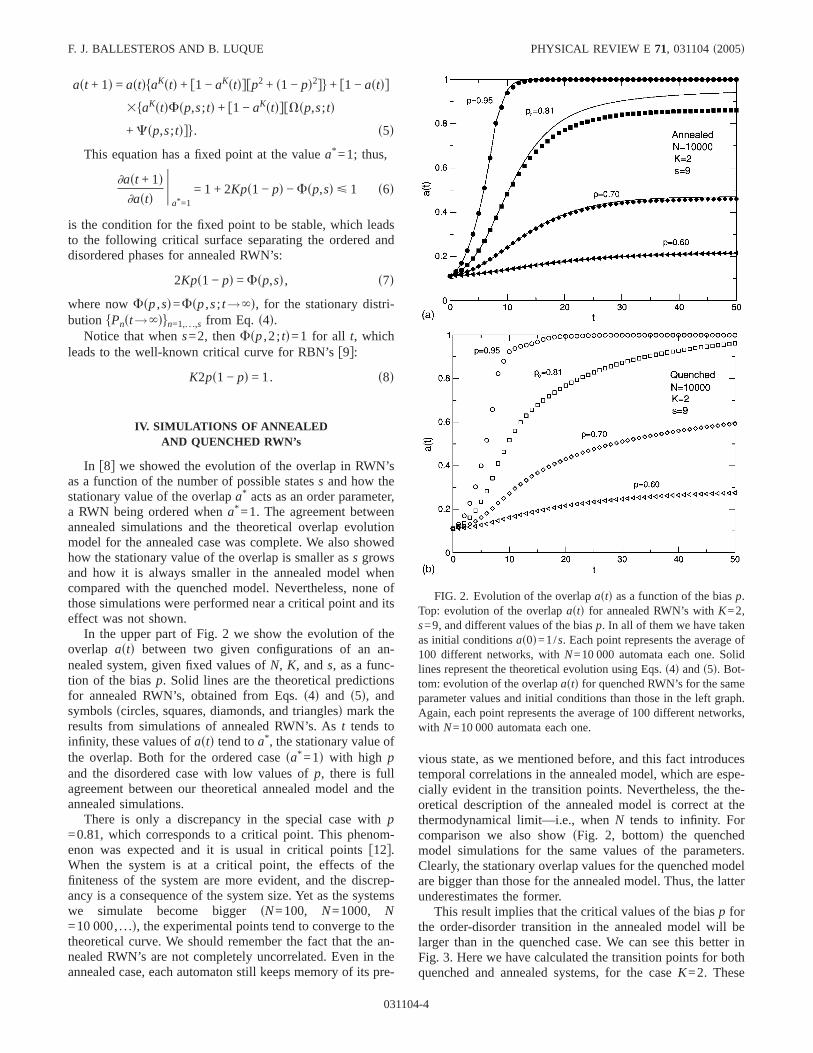
In the upper part of Fig. 2 we show the evolution of theoverlap astd between two given configurations of an an-nealed system, given fixed values ofN, K, ands, as a func-tion of the biasp. Solid lines are the theoretical predictionsfor annealed RWN’s, obtained from Eqs.s4d and s5d, andsymbolsscircles, squares, diamonds, and trianglesd mark theresults from simulations of annealed RWN’s. Ast tends toinfinity, these values ofastd tend toa* , the stationary value ofthe overlap. Both for the ordered casesa* =1d with high pand the disordered case with low values ofp, there is fullagreement between our theoretical annealed model and theannealed simulations.

There is only a discrepancy in the special case withp=0.81, which corresponds to a critical point. This phenom-enon was expected and it is usual in critical pointsf12g.When the system is at a critical point, the effects of thefiniteness of the system are more evident, and the discrep-ancy is a consequence of the system size. Yet as the systemswe simulate become biggersN=100, N=1000, N=10 000, . . .d, the experimental points tend to converge to thetheoretical curve. We should remember the fact that the an-nealed RWN’s are not completely uncorrelated. Even in theannealed case, each automaton still keeps memory of its pre-

vious state, as we mentioned before, and this fact introducestemporal correlations in the annealed model, which are espe-cially evident in the transition points. Nevertheless, the the-oretical description of the annealed model is correct at thethermodynamical limit—i.e., whenN tends to infinity. Forcomparison we also showsFig. 2, bottomd the quenchedmodel simulations for the same values of the parameters.Clearly, the stationary overlap values for the quenched modelare bigger than those for the annealed model. Thus, the latterunderestimates the former.

This result implies that the critical values of the biasp forthe order-disorder transition in the annealed model will belarger than in the quenched case. We can see this better inFig. 3. Here we have calculated the transition points for bothquenched and annealed systems, for the caseK=2. These

FIG. 2. Evolution of the overlapastd as a function of the biasp.Top: evolution of the overlapastd for annealed RWN’s withK=2,s=9, and different values of the biasp. In all of them we have takenas initial conditionsas0d=1/s. Each point represents the average of100 different networks, withN=10 000 automata each one. Solidlines represent the theoretical evolution using Eqs.s4d ands5d. Bot-tom: evolution of the overlapastd for quenched RWN’s for the sameparameter values and initial conditions than those in the left graph.Again, each point represents the average of 100 different networks,with N=10 000 automata each one.

F. J. BALLESTEROS AND B. LUQUE PHYSICAL REVIEW E71, 031104s2005d

031104-4

transition points are defined by the values ofp where a*

equals 1 for the first timeswe can use in fact 1−a* as theorder parameterd. It is clear that the annealed model fails topredict the transition for the quenched model. The transitionin the quenched model takes place at values ofp smaller thanthose predicted by the annealed model predicts and hence, inthis case, Derrida’s method does not work. This failure is aneffect of the different state probability distributionshPnjn=1,. . .,s in both models due to the memory of thequenched system, as we will prove in Sec. V.

Nevertheless, it is important to highlight that in both casesssee Fig. 3d ass increases the curves quickly converge to alimiting value. This implies that at the continuous limit,s→`, the transition is well defined and independent of thevalue ofs f8g.

V. RWN QUENCHED MODEL

In RBN’s the frontier between order and disorder obtainedusing an annealed model coincides with the frontier for thequenched model. As we have seen, this is not the case forRWN’s, and the transitions between order and disorder inthese two models do not coincide. Such a result is due to thefact that the memory of the quenched system introducesstrong correlations in the automata. As a consequence, in thequenched model each automaton is not strictly modified by apure random-walk perturbation, and the automatom-state dis-tributions in this model are clearly different to the distribu-tions in the annealed method. Observe that the stationaryvalues ofhPnjn=1,. . .,s can be calculated from Eq.s4d in thelimit when t→` and then summing up all the equationsfrom 1 to a certainn. In this way we arrive to the followingrecurrent relationship:

Pn = Pn−1S p

1 − pD . s9d

Normalizing to 1 the sum ofPn from 1 to s, we obtain

Pn =1

zS p

1 − pDn−1

, s10d

an exponential discrete probability distribution, with the nor-malization factor equal to

z=

1 −S p

1 − pDs

1 −p

1 − p

. s11d

FIG. 4. The stationary automaton-state distributionhPnjn=1,. . .,6 for a quenched RWN in the cases=6 as a function of the biasp and theconnectivityK. Ordered states are plotted as black bars.

FIG. 3. Order-disorder transition in RWN’s. The critical valuesof the bias for RWN’s withK=2 are plotted as a function of thenumber of statess, for both annealed and quenched systems. Thetransition in quenched RWN’s happens at values ofp smaller thanthose predicted by the annealed model.

ORDER-DISORDER PHASE TRANSITION IN RANDOM-… PHYSICAL REVIEW E 71, 031104s2005d

031104-5

But in fact, the behavior of the automata in the orderedzone is far away from such a biased random walk. The sta-tionary quenched distribution of the automaton values willnot be an exponential like the one described by the previousequation.

Figure 4 shows the stationary automatom-state distribu-tion hPnjn=1,. . .,6 for a quenched RWN in the cases=6. It canbe seen that as we enter the disordered zonesi.e., big valuesof the connectivityKd it tends to an exponential distribution,according to Eq.s10d. In that zone, each automaton is beingperturbed by a nearly pure biased random walk. But in theordered zonessmall values of the connectivityd, the distribu-tion tends to be limited basically to the extreme values, 1 ors, the intermediate states having a probability close to 0. Onecan see how the ordered state has basically a binary outcome.Notice also that in this zone the probability for an automatonto bes or 1 is clearly determined by the biasp, beingp ands1−pd, respectively.

If we now use the stationary quenched values of the au-tomata distribution in the ordered zone—that is, if we use

Pn = 5s1 − pd if n = 1,

p if n = s,

0 otherwise,6 s12d

and we apply them to Eq.s7d, we obtain that the boundarycondition becomes

K2ps1 − pd = 1, s13d

that is, again, the boundary condition for RBN’s.Therefore, RBN’s and the annealed model of RWN’s are

the limiting cases for quenched RWN’sscoinciding only inthe cases=2d, and the critical transition order-disorder curvefor quenched systems lies between both transition frontiercurves, as can be seen in Fig. 5.

As Fig. 3 implies, when passing from these discrete net-works to the continuous case—that is, whens tends toinfinity—the transition from order to disorder is still welldefined. It is possible to calculate the limit of Eq.s7d forannealed RWN’s whens→`. In the continuous case, thecritical curve becomes

K =2fp − s1 − pdg2

ps1 − pdf1 + up − s1 − pdug2 , s14d

which defines an order-disorder critical curve in theK−pspacesFig. 5, dashed lined. Equations13d can be expressed ina more compact form, but we prefer to write it this waybecause it explicitly shows its invariance under the ex-changes ofp and s1−pd.

As the annealed model is a lower limitsin the K axis;upper in thep axisd of the quenched systems, then forquenched RWN’s in the continuous limitss→`d the transi-tion is also well defined and enclosed between the annealedmodel and the classical transition for RBN’s.

VI. CONCLUSIONS

The study of the genome has revealed a complex world ofrelationships and couplings among genes, which produceswhat is indeed a genetic network. As a consequence, thestudy of its behavior by means of classical, linear methods isnot possible given that the real behavior is highly nonlinearand shows complex dynamics. Therefore new type of modelsand methods of analysis are needed to face its study andunderstanding.

RBN’s were one of the first ways proposed to study sta-tistically genome global properties. Unfortunately this is amodel of all-nothing behavior where the state of a givengene is completely determined by the input genes and wheresmooth variations of state are not allowed, contrary to whathappens in the real genomes. On the other hand, differentialequation systems, which in principle should give a betterunderstanding of such continuous behavior, are difficult tosolve and analytical results are hard to obtain.

This paper deals with random walk networks, a simplerandom network model which largely resembles real geneticnetworks. RWN’s are a natural link between discrete all-nothing modelsslike RBN’sd and continuous differentialequations systems, as RWN’s allow small, continuouslikevariations in the behavior of the genome.

RWN’s allow for analytical treatment, and in this paperwe have deduced the critical frontier for the annealed model.Unfortunately, due to the memory of the system, the an-nealed solution does not coincide with the quenched criticalfrontier. Nevertheless, the annealed critical boundary acts asa lower limit for the real case. On the other hand, we have

FIG. 5. Gray pixels: stationary overlapa* between twoquenched RWN’s as a function ofp andK. Gray intensities indicatedifferent values of the stationary overlap. Dark gray corresponds toa perfect overlap—that is, toa* =1 sordered phased—and white tononcorrelateda* scompletely disordered phased. For each point wehave performed 10 000 simulations withN=10 000 ands=4. Su-perimposed are the order-disorder frontiers for RBN’ssupper solidlined and for the annealed model of RWN’sslower solid lined in thecases=4. We can see how the transition from order to disorder inthe quenched RWN’s happens in the zone between both curves. Thedashed line corresponds to the criticalK-p curve from Eq.s12d inthe annealed case whens→`.

F. J. BALLESTEROS AND B. LUQUE PHYSICAL REVIEW E71, 031104s2005d

031104-6

shown how RBN’s act as an upper limit for the quenchedcase and we have delimited its order-disorder transition fron-tier to be between both transition frontiers. If RWN’s pretendto be a bridge model between RBN’s and continuous models,we have demonstrated that in the continuous limitss tendingto infinityd RWN’s are well behaved and, as RBN’s, have awell-defined order-disorder transition, usually so difficult toprove for continuous systems.

As we have seen, RWN’s can be considered a naturalgeneralization of RBN’s. In fact, RBN’s are a subcase of ourmodel which trivially reduce to them when the number ofallowed statess equals 2. RBN’s have been studied exten-sively over the past three decadesf13g and are still used as a

model to study competitive gamesf14g, synchronizationf15,16g, scale-free connectivityf17,18g, self-organized criti-cality f19g, or time-reversible modelsf20,21g. RWN’s nowoffer a more general and richer frame to study all these phe-nomena.

ACKNOWLEDGMENTS

We would like to thank Amelia Ortiz and Alberto Fernán-dez for their valuable opinions. B.L. has been supported byCICYT BFM2002-01812. F.B. has been supported by MECAYA 2003-08739-c02-0sincluding FEDERd and GeneralitatValenciana GRUPOS 03/170.

f1g S. Bornholdt, Biol. Chem.382, 1289s2001d.f2g S. A. Kauffman, J. Theor. Biol.22, 437 s1969d.f3g S. A. Kauffman, The Origins of OrdersOxford University

Press, New York, 1993d.f4g D. Kaplan and L. Glass,Understanding Nonlinear Dynamics

sSpringer-Verlag, New York, 1995d.f5g T. A. Brown, GenomessWiley, New York, 1999d.f6g R. Thomas, D. Thieffry, and M. Kaufman, Bull. Math. Biol.

57, 247 s1995d.f7g K. Kappler, R. Edwards, and L. Glass, Signal Process.83, 789

s2003d.f8g B. Luque and F. Ballesteros, Physica A342, 207 s2004d.f9g B. Luque and R. V. Solé, Phys. Rev. E55, 257 s1997d.

f10g T. Rohlf and S. Bornholdt, Physica A310, 245 s2002d.f11g J. A. de Sales, M. L. Martins, and D. A. Stariolo, Phys. Rev. E

55, 3262s1997d.

f12g B. Derrida and Y. Pomeau, Europhys. Lett.1, 45 s1986d.f13g M. Aldana, S. Coppersmith, and L. P. Kadanoff, inPerspec-

tives and Problems in Nonlinear Science, Springer AppliedMathematical Sciences Series, edited by E. Kaplan, J. E. Mars-den, and K. R. SreenivasansSpringer-Verleg, Berlin, 2003d.

f14g I. Nakamura, Phys. Rev. E65, 046128s2002d.f15g L. G. Morelli and D. Zanette, Phys. Rev. E63, 036204s2001d.f16g F. J. Ballesteros and B. Luque, Physica A313, 289 s2002d.f17g J. J. Fox and C. C. Hill, Chaos11, 809 s2001d.f18g C. Oosawa and M. A. Savageau, Physica D170, 143 s2002d.f19g B. Luque, F. J. Ballesteros, and E. M. Muro, Phys. Rev. E63,

051913s2001d.f20g S. N. Coppersmith, L. P. Kadanoff, and Z. Zhang, Physica D

149, 11 s2001d.f21g S. N. Coppersmith, L. P. Kadanoff, and Z. Zhang, Physica D

157, 54 s2001d.

ORDER-DISORDER PHASE TRANSITION IN RANDOM-… PHYSICAL REVIEW E 71, 031104s2005d

031104-7