Optimization of Water Allocation, Wastewater Treatment ...
131
Utah State University Utah State University DigitalCommons@USU DigitalCommons@USU Reports Utah Water Research Laboratory January 1975 Optimization of Water Allocation, Wastewater Treatment, and Optimization of Water Allocation, Wastewater Treatment, and Reuse Considering Nonlinear Costs, Seasonal Variations, and Reuse Considering Nonlinear Costs, Seasonal Variations, and Stochastic Supplies Stochastic Supplies A. Bruce Bishop Rangesan Narayanan Suravuth Pratishthananda Stanley L. Klemetson William J. Grenney Follow this and additional works at: https://digitalcommons.usu.edu/water_rep Part of the Civil and Environmental Engineering Commons, and the Water Resource Management Commons Recommended Citation Recommended Citation Bishop, A. Bruce; Narayanan, Rangesan; Pratishthananda, Suravuth; Klemetson, Stanley L.; and Grenney, William J., "Optimization of Water Allocation, Wastewater Treatment, and Reuse Considering Nonlinear Costs, Seasonal Variations, and Stochastic Supplies" (1975). Reports. Paper 601. https://digitalcommons.usu.edu/water_rep/601 This Report is brought to you for free and open access by the Utah Water Research Laboratory at DigitalCommons@USU. It has been accepted for inclusion in Reports by an authorized administrator of DigitalCommons@USU. For more information, please contact [email protected].
Transcript of Optimization of Water Allocation, Wastewater Treatment ...
Utah State University Utah State University
DigitalCommons@USU DigitalCommons@USU
Reports Utah Water Research Laboratory
January 1975
Optimization of Water Allocation, Wastewater Treatment, and Optimization of Water Allocation, Wastewater Treatment, and
Reuse Considering Nonlinear Costs, Seasonal Variations, and Reuse Considering Nonlinear Costs, Seasonal Variations, and
Stochastic Supplies Stochastic Supplies
A. Bruce Bishop
Rangesan Narayanan
Suravuth Pratishthananda
Stanley L. Klemetson
William J. Grenney
Follow this and additional works at: https://digitalcommons.usu.edu/water_rep
Part of the Civil and Environmental Engineering Commons, and the Water Resource Management
Commons
Recommended Citation Recommended Citation Bishop, A. Bruce; Narayanan, Rangesan; Pratishthananda, Suravuth; Klemetson, Stanley L.; and Grenney, William J., "Optimization of Water Allocation, Wastewater Treatment, and Reuse Considering Nonlinear Costs, Seasonal Variations, and Stochastic Supplies" (1975). Reports. Paper 601. https://digitalcommons.usu.edu/water_rep/601
This Report is brought to you for free and open access by the Utah Water Research Laboratory at DigitalCommons@USU. It has been accepted for inclusion in Reports by an authorized administrator of DigitalCommons@USU. For more information, please contact [email protected].
OPTIMIZATION OF WATER ALLOCATION, WASTEWATER TREATMENT, AND REUSE
CONSIDERING NONLINEAR COSTS, SEASONAL VARIATIONS,
AND STOCHASTIC SUPPLIES
by
A. Bruce Bishop Rangesan Narayanan
Suravuth Pratishthananda Stanley L. :Klemetson WUliam J. Grenney
The work upon which this report is based was supported in part by funds provided by the Department of the Interior, Offtce of Water Research and Technology, as authorized under the Water Resources Research Act' of 1964, PubUc Law 88-379, Project No. B-097-Utah, Agreement No. 14-31-0001-4133.
Utah Water Research Laboratory College of Engineering Utah State University Logan, Utah 84322
June 1975 PRWGI23-2

ABSTRACT
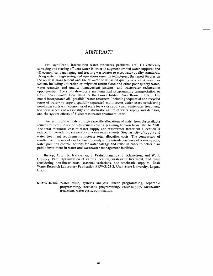
Two significant, interrelated water resources problems are: (1) efficiently salvaging and reusing effluent water in order to augment limited water supplies; and (2) economically managing and treating wastewater to meet water quality standards. Using systems engineering and operations research techniques, the report focuses on the optimal management and use of water of imparied quality in a water resources system, including utilization or irrigation return flows and other poor quality water, water quantity and quality management systems, and wastewater reclamation opportunities. The study develops a mathematical programming transportation or transhipment model formulated for the Lower Jordan River Basin in Utah. The model incorporated all "possible" water resources (including sequential and recycled reuse of water) to supply spatially separated multi-sector water users considering non-linear costs with economies of scale for water supply and wastewater treatment, temporal aspects of seasonality and stochastic nature of water supply and demand, and the system effects of higher wastewater treatment levels.
The results of the model runs give specific allocations of water from the available sources to meet use sector requirements over a planning horizon from 1975 to 2020. The total minimum cost of water supply and wastewater treatment allocation is reduced by considering seasonality of water requirements. Stochasticity of supply and water treatment requirements increase total allocation costs. The comparison of results from the model can be used to analyze the interdependence of water supply, water pollution control, options for water salvage and reuse in order to better plan public investment in water and wastewater management facilities.
Bishop. A. B., R. Narayanan, S. Pratishthananda, S. Klemetson, and W. J. Grenney, 1975. Optimization of water allocation, wastewater treatment, and reuse considering non-linear costs, seasonal variations, and stochastic supplies. Utah Water Research Laboratory Publication PRWG123-2, Utah State University, Logan, Utah.
KEYWORDS: Water reuse, systems analysis, linear programming, separable programming, stochastic programming, water supply, wastewater treatment, water costs, optimization.
iii

ACKNOWLEDOMENTS
This publication is the final report of a prdjed which was stippotted hi part with funds provided by the Office of Water Resources Research 6f the. United States Department of the Interior as authorized under the Water Resoutces Research Act of 1964. Public Law 88-379. The work was accomtHis}i(!d by personnel of the Utah Water Research Laboratory, Utah State UhivehitY.

TABLE OF CONTENTS
Chapter Pap
I. WATER REUSE-SYSEMATIC APPROACHES ........................ 1
Water Reuse in Water Resource Planning ............................ 1 Previous Work-Model Formulation and Results ..................... 1 Further Analyses of W ater Reus~Model Modifications ............... 3 Relation of Study to Current Literature .............................. 4
Linear programming applications ............................. .4 Dynamic programming ....................................... 5 Nonlinear programming ...................................... 5 Multilevel optimization ....................................... 6 Integer and mixed-integer programming ......................... 6
II. MODEL REVISION FOR ANALYSIS OF WATER REUSE IN WATER RESOURCES SYSTEMS .................................. 7
Modifications in the Basic Transportation Model of Water Reuse ................................................ 7
Nonlinear cost formulation .................................... 7
Separable Programming Model .................................... 9
Seasonal variations in the model parameters ..................... 11
Stochastic Considerations ........................................ 11 Summary of Model Runs for the Case Study Area .................... 11
III. WATER RESOURCES A V AILABILITY, WATER REQUIREMENTS, AND WATER REUSE COSTS ...................... 13
Surface Streams Water .......................................... 13
Jordan river ................................................ 13 The wasatch front streams .................................... 13
Groundwater ................................................... 13 Imported Water ................................................ 13 Effluent Sources ................................................ 14 Water Quality .................................................. 14 Water Requirements ............................................ 14
Municipal requirements ..................................... 14 Industrial uses ............................................. 15 Agricultural uses ........................................... 15
Water Reuse Costs .............................................. 17

IV. MODELOPERAttON ANDCd:M:t>ARISONdFREStJLfs .............. 27
Comparative Analysis of MOdel Runs: ............................. .27 Analysis of Results for Model Structtih~s ............................ 27
Spatial aggregation verstis~isag~eg~tioh .. ~ ..................... 27 Effect of higher disch~rge quality t~ijuit~mbitS ., ................ is Seasortal variatioiis ... , .... ,' .................................. ~~ Linear vs. nonliriear cost ftinction: ............................. 3~ Deterministic vs. stOChastic ni(j(:t~ls ............................ 33 Sector allocations under va.riousi.sstIT,~Hdiis .................... j" Surface water and water treattneht pUints ....................... 37 Groundwater ............................................... ~7 Reusable sources ........................................... 3,7
Imported water .................................................. 3~ Reuse patterns and imported w~tet ............................ 38 Wastewater treatrilent plarlts ................................. 39
Computer Tiine/Cost Companstins ................................ 40
REFERENCES .......... ' ............................................... 4i
APPENDICES ...................................... , : ................. 4j
AP~ENDIX A ..................................................... 45 APPENDIX B ................................................. ~ .. r 1~ APPENDIX C .................................................... 117
vi

LIST OF FIGURES
Figure Pap
1. Model illustration for linear costraints and concave objective function for two-variable case ......................................... 8
2. Illustration of global minimum and multiple optima for linear constraint 2. Illustration of global minimum and multiple optima for
Hnear constraint concave objective function example ...................... 8
3. Illustration of the problem of a relative optimum solution for the linear constraint--concave objective function problem ................. 9
4. Piecewise linearization of a nonHnear cost function ...................... 10
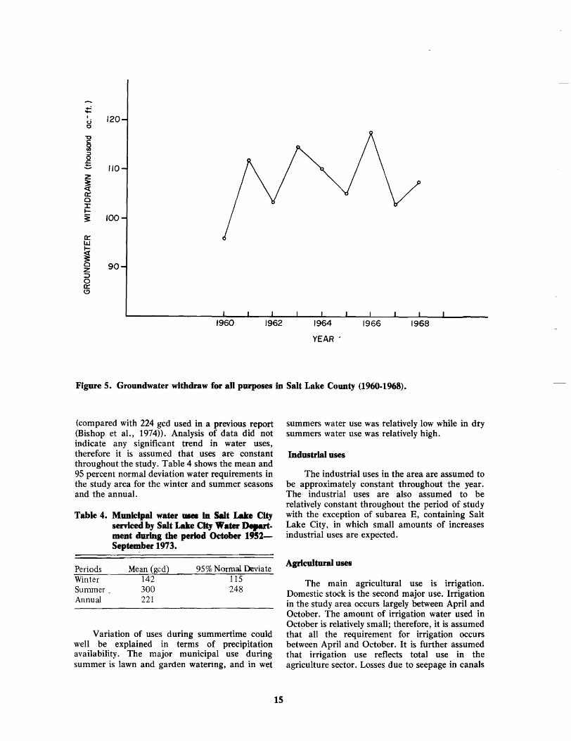
5. Groundwater withdraw for all purposes in Salt Lake County (1960-1968) ....................................................... 15
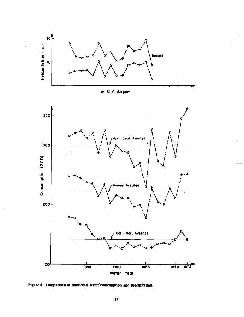
6. Comparison of municipal water consumption and precipitation ............ 16
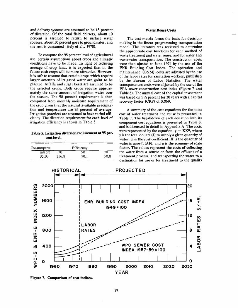
7. Comparison of cost indices ......................................... 17
8. WWTP utiHzation in 2020 under existing water quality standard ......................................................... 28
9. Wastewater reuse flows resulting from higher level treatment requirements, 1980 ................................................. 29
10. Wastewater and water reuse flows resulting from higher level treatment requirements, 1985 ........................................ 29
11. Wastewater and water reuse flows resulting from higher level treatment requirements, 2000 ........................................ 30
12. Wastewater and water reuse flows resulting from higher level treatment requirements, 2020 ......................................... 30
13. Comparison of total minimum cost of optimal allocation under various model assumptions ..................................... 31
14. Comparison of total minimum cost of optimal allocation for annual versus seasonal model runs .................................... 33
15. Waste treatment utilization and reuse pattern for 1975 with quality level I ...................................................... 35
16. Waste treatment utilization and reuse pattern for 1980 with quality level II ..................................................... 3S
vII
LIST OF FIGURES (Continued)
. 17. Waste treatment utilization and reuse pattern for 1985 with quality level III .................................................... 36
18. Waste treatment utilization and reuse pattern in 2000 with quality level III .................................................... 36
19. Waste treatment utilization and reuse pattern for 2020 with quality level III .................................................... 37
LIST OF TABLES
Table Page
1. Summary of model runs under various model structures .................. 12
2. Surface water availability in Salt Lake County .......................... 14
3. Estimated safe yield of groundwater in each subarea of the study ..... ',' ..................................................... 14
4. Municipal water uses in Salt Lake "City serviced by Salt Lake City Water Department during the period October 1952-Septem ber 1973 ................................................... 15
S. Irrigation diversion requirement at 95 percent level ...................... 17
6. Cost indices ....................................................... 18
7. Total water treatment and reuse cost equationa, y = ,KKa ................ 19
8. Summary of cost equation a .......................................... 20
9. Runs used for comparison of results for various model structures ........... 27
10. Annual cost comparison of optimal allocation ........................... 31
11. Wastewater treatment plants utilization ............................... 34
12. Replacement of surface water by import water in optimal solutions for stochastic model ........................................ 34
13. Water treatment plants (maximum capacity 209,700 ac-ft/year) ........... 37
14. Groundwater withdrawal pattern ..................................... 38
15. Reuse pattern: deterministic and stochastic ............................ 38
16. Import water better than Class C (ac-ft/year) ........................... 38
17. Reuse comparisons: Linear vs. nonlinear model, municipal and industrial effluent for M, I, and agricultural uses .................... 39
18. Import water comparisons between linear and nonlinear models (municipal use) ............................................. 39
19a. Required wastewater treatment plants capacity (100 ac-ft/year) (a) existing quality: annual vs. seasonal ................................ 39
19b. Required wastewater treatment plants capacity (100 ac-ft/year) (b) higher quality: annual vs. seasonal ................................. 39
Ix

CHAPTER I
WATER REUSE-SYSTEMATIC APPROACHES
Water Reuse in Water Resources Planning
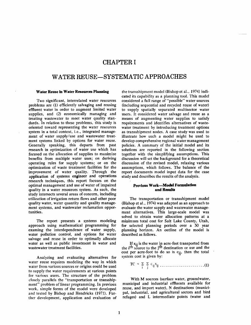
Two significant, interrelated water resources problems are (1) efficiently salvaging and reusing effluent water in order to augment limited water supplies, and (2) economically managing and treating wastewater to meet water quality standards. In relation to these problems, this study is oriented toward representing the water resources system in a total context, i.e., integrated management of water supply/use and wastewater treatment systems linked by options for water reuse. Generally speaking, this departs from past research in optimization of water use which has focused on the allocation of supplies to maximize benefits from multiple water uses; on deriving operating rules for supply systems; or on the optimization of waste treatment facilities for the improvement of water quality. Through the application of systems engineer and operations research techniques, this report focuses on the optimal management and use of water of impaired quality in a water resources system. As such, the study intersects several areas of concern, including utilization of irrigation return flows and other poor quality water, water quantity and quality management systems, and wastewater reclamation opportunities.
The report presents a systems modeling approach using mathematical programming for examing the interdependence of water supply, water pollution control, and options for water salvage and reuse in order to optimally allocate water as well as public investment in water and wastewater treatment facilities.
Analyzing and evaluating alternatives for water reuse requires modeling the way in which water from various sources or origins could be used to supply the water requirements at various points for various users. The structure of the problem c10sely parallels the "transportation or transshipment" problem of linear programming. In previous work, simple forms of the model were developed and tested by Bishop and Hendricks (1971). Further development, application and evaluation of
1
the transshipment model (Bishop et aI., 1974) indicated its capability as a planning tool. This model considered a full range of "possible" water sources (including sequential and recycled reuse of water) to supply spatially separated multisector water users. It considered water salvage and reuse as a means of augmenting water supplies to satisfy requirements and identifies alternatives of wastewater treatment by introducing treatment options as transshipment nodes. A case study was used to illustrate how such a model might be used to develop comprehensive regional water management policies. A summary of the initial model and its solutions are reported in the following section together with the simplifying assumptions. This discussion will set the background for a theoretical discussion of the revised model, relaxing various assumptions, which follows. The balance of the report documents model input data for the case study and describes the results of the analysis.
Previous Work-Model Formulation and Results
The transportation or transshipment model (Bishop et aI., 1974) was adapted as an approach to evaluate the water supply and wastewater management alternatives. This large-scale model was solved to obtain water allocation patterns at a minimum total cost for Salt Lake County, Utah, for selected planning periods over a 50 year planning horizon. An outline of the model is described as follows.
IfXij is the water in acre-feet transported from the ith source to the jth destination or use and the cost per acre-foot to do so is Cij' then the total system cost is given by:
TC ~ ~ c .. x.. (1) j IJ IJ ••.•••••••••••••••••••
With M sources (surface water, groundwater, municipal and industrial effluents available for reuse, and import water), N destinations (municipal, industrial, and agricultural sectors and bird refuges) and L intermediate points (water and
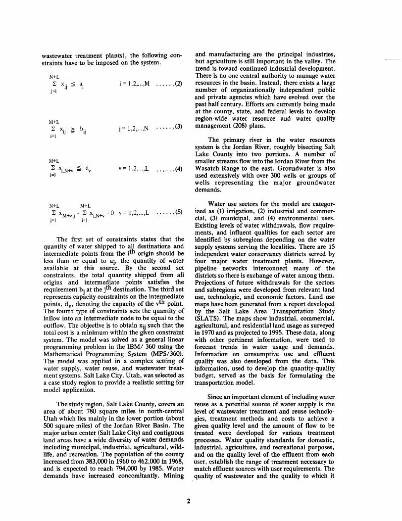
wastewater treatment plants), the following constraints have to be imposed on the system.
N+L
L x .. ~ ai j=l
IJ
M+L
L x ij ~ bij i=l
M+L
L \N+v ~ dv i=l
N+L M+L
i = 1,2, ... ,M ...... (2)
j = 1,2, ... ,N ...... (3)
v = 1,2, ... ,L ...... (4)
L xM+v,j - L xi,N+v = 0 V = 1,2, ... ,L ...... (5) j=l i=l
The first set of constraints states that the quantity of water shipped to all destinations and intermediate points from the ith origin should be less than or equal to ai, the quantity of water available at this source. By the second set constraints, the total quantity shipped from all origins and intennediate points satisfies the requirement bj at the jth destination. The third set represents capacity constraints on the intennediate points, dv' denoting the capacity of the vth point. The fourth type of constraints sets the quantity of inflow into an intetmediate node to be equal to the outflow. The objective is to obtain Xij such that the total cost is a minimum within the glVen constraint system. The model was solved as a general linear programming problem in the IBM/ 360 using the Mathematical Programming System (MPS/360). The model was applied in a complex setting of water supply, water reuse, and wastewater treatment systems. Salt Lake City, Utah, was selected as a case study region to provide a realistic setting for model application.
The study region, Salt Lake County, covers an area of about 780 square miles in north-central Utah which lies mainly in the lower portion (about SOO square miles) of the Jordan River Basin. The major urban center (Salt Lake City) and contiguous land areas have a wide diversity of water demands including municipal, industrial, agricultural, wildlife, and recreation. The popUlation of the county increased from 383,000 in 1960 to 462,000 in 1968, and is expected to reach 794,000 by 1985. Water demands have increased concomitantly. Mining
2
and manufacturing are the principal industries, but agriculture is still important in the valley. The trend is toward continued industrial development. There is no one central authority to manage water resources in the basin. Instead, there exists a large number of organizationally independent public and private agencies which have evolved over the past half century. Efforts are currently being made at the county, state, and federal levels to develop region-wide water resource and water quality management (208) plans.
The primary river in the water resources system is the Jordan River, roughly bisecting Salt Lake County into two portions. A number of smaller streams flow into the Jordan River from the Wasatch Range to the east. Groundwater is also used extensively with over 300 wells or groups of wells representing the major groundwater demands.
Water use sectors for the model are categorized as (1) irrigation, (2) industrial and commercial, (3) municipal, and (4) environmental uses. Existing levels of water withdrawals, flow requirements, and influent qualities for each sector are identified by subregions depending on the water supply systems serving the localities. There are 15 independent water conservancy districts served by four major water treatment plants. However, pipeline networks interconnect many of the districts so there is exchange of water among them. Projections of future withdrawals for the sectors and subregions were developed from relevant land use, technologic, and economic factors. Land use maps have been generated from a report developed by the Salt Lake Area Transportation Study (SLATS). The maps show industrial, commercial, agricultural, and residential land usage as surveyed in 1970 and as projected to 1995. These data, along with other pertinent infonnation, were used to forecast trends in water usage and demands. Information on consumptive use and effluent quality was also developed from the data. This infonnation, used to develop the quantity-quality budget, served as the basis for fonnulating the transportation model.
Since an important element of including water reuse as a potential source of water supply is the level of wastewater treatment and reuse technologies, treatment methods and costs to achieve a given quality level and the amount of flow to be treated were developed for various treatment processes. Water quality standards for domestic, industrial, agriculture, and recreational purposes, and on the quality level of the effluent from each user, establish the range of treatment necessary to match effluent sources with user requirements. The quality of wastewater and the quality to which it
must be upgraded to meet specified uses, are analyzed in selecting unit treatment costs to be used in the transportation model. The costs include the costs of the various stages of treatment processes taking into account the capital, operating and maintenance costs for each stage with respect to the plant capacity.
The modeling effort was directed toward developing an operating model and applying it to a water resources system. All basic components of the system were incorporated into the model including water supply sources, use sectors (municipal, industrial, agriculture, etc.) effluents for reuse, and wastewater treatment operations.
The results of the optimal system configuration pertained to the resource use patterns over time. In the study area, the water treatment plants appeared to have ample excess capacity and can be expected to meet peak flows even in year 2020. Central Utah Project water, an import source for the county, was not needed until year 2000. Groundwater withdrawal seemed to be lower than the safe yield and the minimum cost solutions showed a shift to more usage of groundwater in the municipal sector and sequential reuse in the agricultural sector under high demand conditions.
Also, the solution gave insight into the wastewater management aspects. With the application of class C standards all over the basin, the existing treatment plants in four of the seven subregions in the county needed expansion according to the model results.
Besides the optimal system configuration, proposals relating to regionalization of waste treatment facilities were examined using the model. Four alternatives of wastewater handling schemes for the case study area were evaluated and the results indicated that a decentralized threeregional plant system was the minimum cost solution.
Further Analyses of Water Reuse--~odel~o~cadoDS
The initial model developments and results just described were based on three types of simplifying assumptions about the system:
1. Average annual water availabilities.
2. Average annual rather than seasonal demands for water supplies.
3. Linearity of unit costs of water treatment and distribution.
3
In the current study the basic transportation model is modified and some simplifying assumptions are relaxed in evaluating water supply and reuse, treatment and pollution control alternatives in a region. An important question is whether or not solutions obtained are significantly different than and an improvement over the simpler model. If so, does the additional information appear to be worth the additional effort in terms of data collection, computational time, and costs?
The approach in carrying out these analyses is summarized as follows:
1. Develop and refine the systems model through disaggregation of the initial model and through expansion of the model to inc1ude seasonal variations and stochasticity in supply, and nonlinearities in cost functions.
The seasonal fluctuation in water supply and use, along with the trend in water requirements from land use change and popUlation growth, is incorporated on a discrete time basis through manipulation of the right-hand sides of the model constraints. The analysis to be derived from the model likewise covers a wider range of questions such as the timing and location of investments on treatment facilities, distribution systems, groundwater withdrawal, and the timing and sequencing in allocation of supplies to satisfy future demands.
The introduction of stochasticity under the dynamic conditions is a further important area of inquiry. Generally, the water available from various supply sources is stochastic as are the requirement levels of various water using sectors. By assigning a proper probability distribution for these values, an optimal pattern of water allocation can be arrived at using stochastic programming techniques in conjunction with the transportation model. Chance constrained programming is applied to deal with situations where extremes are considered significant.
Recognizing that cost functions are usually nonlinear functions of the quantity of water treated or transported, techniques to account for nonlinearities are employed within the transportation model in order to yield more accurate results. Separable programming is used to deal with nonlinearities in costs while maintaining the relative simplicity of a linear programming analysis.
2. Examine various alternatives for water reuse by estimating the least cost method for satisfying projected levels of water use while meeting water quality standards.

With the expanded and disaggregated model for the study area, various alternatives for meeting water demands through wastewater reuse are analyzed. Least cost allocation patterns under various assumptions and constraints for operating the system are derived and compared. A number of important questions are analyzed in evaluating alternatives to identify least cost optimal allocation patterns for both spatial and temporal considerations. Some of these include: Is it more efficient to reuse water directly from effluent source to subsequent user or to treat wastewater at a central treatment plant and then redistribute it? How does water salvage and reuse compare with other alternative water sources such as importation or increased pumpage of groundwater reservoirs? What is the impact of water salvage and reuse on the overall costs in meeting federal and state water quality standards?
By analyzing such questions the model's capability for testing water supply and wastewater management strategies can be examined. The modeling methodology is illustrated through its application to an actual study area in order to assess its usefulness as a planning tool. This involves three areas of concern:
a. Institutional restrictions on resource allocation, in particular, pollution standards.
Water supply, as well as pollution control, operates in a mileau of institutional restrictions, often spelled out as legal requirements. Pollution standards are one such restriction. The cost of these restrictions can be evaluated by obtaining optimal solutions with and without the higher levels of treatment required by water quality standards.
b. The optimal scale as well as the timing and sequence of investment in the various facilities.
Cost functions for storage, transportation, and treatment are generally nonlinear because of scale economies and initial operation of plants below design capacities. Nonlinear relationships are incorporated into the model as linear approximations to get a more accurate solution for economic size and scale of operation of water supply and treatment facilities.
To investigate the timing of investments and the phasing-in of facilities in various locations to meet user needs, the transportation model is set in a dynamic framework simulating time by using parametric programming techniques to simulate changes in water use over time. In this way, a
4
multi-year analysis is carried out to determine the need to build new facilities in the future.
c. The usefulness of the model for generalized application to the optimization of water supply, water reuse, and wastewater treatment systems.
The studies and analyses performed in the research are directed toward current questions of water planning and development agencies. The adequacy of the system model is assessed and conclusions drawn with regard to future water planning in a region. Present or projected demands exceed the available supply of groundwater and existing surface water sources in many parts of the country. In these water short areas water reuse should be an important consideration in extending available water supplies. The study area, the integrated urban and agricultural complex along the Wasatch Front of Utah, provides an opportune setting for systems evaluation of water reuse because it is a relatively closed system in which data can be obtained and in which exists a wide range of water management problems and alternatives.
Relation of Study to Current Literature
The use of mathematical programming models in the field of water management has been quite extensive. Various optimization techniques have found application in wastewater management, specifically, in the design of treatment plants, achieving a stipulated regional water quality goal, staging an expansion of treatment facilities, and in analyzing the problem of investment timing for the region as a whole. The application of programming models in water supply planning has been generally restricted to minimum cost allocation of municipal water. Attempts to incorporate an exhaustive set of alternatives in a multi-source, multi-sector framework, described for this study, have been made only by a few.
Linear programming appUcations
Linear programming (LP) is one of the most widely used optimization techniques. The popularity of LP formulation is not only in the conceptual simplicity but also the readily available software packages on computers that can efficiently handle large numbers of variables and constraints in the problem. Lynn et al. (1962) used linear programming techniques to derive the combination of treatment processes that minimize cost in removing given amounts of BOD, and also (Lynn, 1964) to solve the capacity expansion problem of waste
treatment facilities subject to the availability of funds, level of treatment required, and quantity of waste.
Loucks et al. (1967) presented two LP models to determine the amount of wastewater treatment required to achieve, at minimum cost, any particular set of stream dissolved oxygen standards for a river by using the Streeter-Phelps equation for DO profile. Using the input-output framework for statewide water resources modeling, Lofting and McGauhey (1968) applied the linear programming technique to optimize allocation of water over time. Clyde et al. (1971) developed a geographical subregion LP approach to statewide water resources planning. Keith et al. (1973) used supplydemand analysis and linear programming to obtain optima] aJIocations in the State of Utah.
LP algorithms can also be used to solve certain classes of quadratic programming. Lynn (1966) set up a programming model to supply weJI water at minimum cost using a quadratic cost function.
LP technique is also used with simulation, another system analysis approach, to obtain optimal allocation. For example, Harl et al. (1971) used a river quality model in conjunction with the LP model such that the results of LP are transmitted to the Fortran river quality simulation model, which in turn alters the parameter of the LP model. The LP problem is resolved using the new parameters, and the solution is fed back to the Fortran subroutine. This process is repeated until changes in the parameters and changes in the LP solution cease.
Dynamic programming
Dynamic programming (DP) has also received wide interest in application to water resources allocation problems. The formulation of a dynamic program need not be linear, continuous, or deterministic. The technique is especially suitable for sequential decision problems. In early applications of DP, Liebman and Lynn (1966) minimized the cost of providing waste treatment to meet a specified DO standard along a stream.
Dynamic programming was employed by Evenson et a). (1969) to solve the two-dimensional multi-stage allocation problem to minimize design costs to remove a desired amount of BOD and to treat and dispose of the solids generated. An optimal investment scheme for water supply projects in response to growing demand conditions was proposed by Butcher et al. (1969) using a dynamic programming approach.
5
Dynamic programming was used to optimize the conjunctive use of ground and surface waters (Aron and Scott, 1971) involving several surface reservoirs, streams, recharge facilities, distribution pipelines, and aquifers. The system was decomposed into several smaller and simpler subsystems. An optimal water allocation policy for 8 years operation in 3-month intervals was obtained.
Hinomoto (1972) makes use of the dynamic programming in planning capacity expansion of water treatment systems. The concave cost function reflecting economies of scale was minimized over the solution space to yield the optimal time and size of plants' capacities. Morin (1973) applied dynamic programming to find the optimum sequencing capacity expansion of water supplies in the Ohio River Basin and the Texas River Basin.
Even though the DP technique is quite flexible and relatively simple in concept, the technique does have disadvantages. The major drawback is its inability to handle, efficiently, more than two decision varables at each stage. Other disadvantages of the technique is the requirement that the objective function and the constraints be formed by sums or pruducts of functions of one decision variable each; solution algorithm is problem dependent, therefore, no general algorithm is available to solve dynamic programming as against linear programming. Sensitivity of the system cannot be analyzed without rerunning the problem.
Nonlinear programming
Nonlinear programming (NP) techniques have been applied to find the least-cost alternative to satisfy water demand within a region (Young and Pisano, 1970). Surface water, groundwater, desalination, and reuse of wastewater were considered as supply sources to satisfy municipal and industrial demands. Nonlinearity was introduced in processes cost and transportation cost. Examination of response surface was used as the technique to find the optimal solution. Walker and Skogerboe (1973) used the Jacobian technique to transform the constrained nonlinear problem into an unconstrained nonlinear problem in the allocation of water resources subjected quality requirements. Bajer (1974) used the differential algorithm to solve nonlinear problems of managing water quality in a river basin.
Application of nonlinear programming has been limited to systems that do not have substantial number of variables. Lack of standard algorithms and available software package is one of the drawbacks of NP techniques.
Multilevel optimization
Windsor and Chow (1972) used multilevel optimization approaches to obtain optimal design of a river basin water resource development. Nonlinear cost of each subsystem is approximated by piecewise linear function. Haimes et al. (1972) applied multilevel approaches to optimize water treatment costs of the region. The lyRem .11 decomposed into 27 subsystems. The system was of linear inequality constraints and quadratic objective functions. Yu and Haimes (1974) obtained optimal policy to manage conjunctive use of groundwater and surface water using multilevel optimization approaches. Haimes and Naiuis (1974) used multilevel approaches to obtain coordination strategy for regional water resources supply and demand.
The concept of multilevel optimization is not new; however, application of this technique to water resources planning and management is relatively recent. The ability to handle any types of optimization and simulation models at lower levels is one of the most attractive features of this approach.
Integer and mixed-integer programming
Another notable optimization technique used in water resources planning and management is integer programming (IP). IP algorithms are used by Liebman and David (1968) to evaluate effectiveness of the three approaches suggested in the literature to achieve water quality goals, viz. the cost minimization approach, uniform treatment approach, and zoned uniform treatment approach. Regev and Schwartz (1973) take up the problem of simultaneous optimization of investment and allocation of water. A discrete time control theory is applied in which interaction of regional and seasonal considerations plays a crucial role. The cost functions reflecting increasing returns to scale
6
were treated as integer variables, so that theoretically a global optimum will be guaranteed.
Cost of development of various components in a water resources system exhibit "economy of scale" characteristics, i.e., as the components increase in size, costs per unit size decrease. The cost function can then be better approximated by a nonlinear function (Koenig, 1967; Linaweaver and Clark, 1964).
There are, strictly speaking, two approaches of handling nonlinearity in the cost function. The first is by using NP technique. The second is by the approximation of the cost function by a number of linear segments then applying a variation of LP algorithm to solve for the optimal.solution.
Mixed integer programming is a combination of integer and linear programming. The technique allows discrete variables to be included in linear programming considerations. Hughes and Clyde (1973) applied the formulation in designing a municipal water supply system utilizing surface and groundwater sources as well as physical aspects of the system. Constraints considered were supply, blending, reservoir, developed facilities, and stochastic constraints. DeVries and Clyde (1971) considered a municipal water supply system utilizing singly or in combination a conventional water supply, a desalted water supply and a supply from a recharged aquifer. The system is also operated in conjunction with an artificially recharged aquifer reservoir. Logarithmic transformation is used to change the nonlinear cost function into ordinary LP formulation. Mulvihill and Dracup (1974) used the concept of inner linearization to approximate the nonlinear cost function. The optimal allocation, sizing, and timing is obtained through iterative procedure.
A standard software package is now available from many computer manufacturers that is capable of solving standard variations of LP formulation such as separable programming and stochastic programming (Burroughs, 1973).
CHAPTER II
MODEL REVISION FOR ANALYSIS OF WATER REUSE IN WATER RESOURCES SYSTEMS
Modifications In the Basic Transportation Model of Water Reuse
The previous chapter outlined the work of an earlier study in which certain simplifying assumptions were made. This chapter describes several model revision, relaxing these simplifying assumptions, and presents their theoretical basis.
Nonllnear cost formulation
The assumption of constant linear costs is unrealistic in that it does not reflect the "fixed charge" nature of the capital stock in the system facilities or the decreasing nature of the total average cost of the system facilities due to economics of scale.
In general, if the cost cii' of supplying the water from the ith source to the Jth user depends on the quantity supplied Xi} then the total cost can be given by
TC = 7 1 Cij (xij ) .................. (6)
Now, the problem is one of minimizing expression (6) subject to constraint sets (2), (3), (4), and (5) indicated in Chapter I. In contrast to the objective function in expression (1), the total cost in (6) is now nonlinear and is estimated as a log-linear relationship of the form,
a .. Cii (x .. ) = A.. x .. IJ Vi, J.
IJ 1] IJ IJ
in which
0< a ij < 1 an d Aij > 0
Therefore, the total cost can be given by
7
a·· TC = L L c.· (x .. ) = L LA .. X .. IJ •• : •• (7)
i j IJ IJ i j IJ IJ
Minimization of (7) subject to the linear constraints (2), (3), (4), and (5) requires a nonlinear programming method.
Before going into the selection of the algorithm to solve such a problem, the qualitative analysis of this problem should be understood. Since the constraint equations are all linear , the set of feasible solutions (if they exist) is a closed convex set bounded from below (due to the non-negativity restrictions). The total cost for any i and j is given by
a·· Cii (xi]·) = Ai]· xji IJ 0 < a·· < 1 (8)
~ ~ IJ •••••••••
Aij > 0
This function is strictly concave in the range 0 < xij < a due to the fact, 1
a.. a·· a.. AI]· A IJ X .. IJ > A.. A x .. IJ for any
IJ IJ IJ
A, 0 < A < 1 ........................ (9)
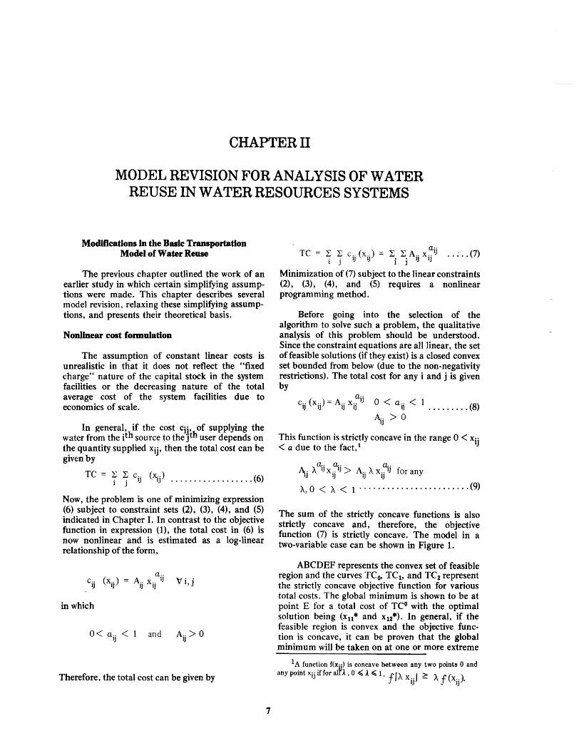
The sum of the strictly concave functions is also strictly concave and, therefore, the objective function (7) is strictly concave. The model in a two-variable case can be shown in Figure 1.
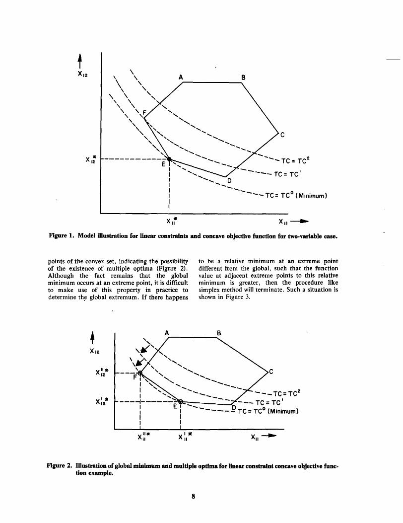
ABCDEF represents the convex set of feasible region and the curves Teo, TC lt and TCz represent the strictly concave objective function for various total costs. The global minimum is shown to be at point E for a total cost of TCo with the optimal solution being (xu* and X 12·) . In general, if the feasible region is convex and the objective function is concave, it can be proven that the global minimum will be taken on at one or more extreme
1 A function f(xli) is concave between any two points 0 and
any point Xij if for alrl. 0 ~ l ~ 1. f[A Xij] ~ A f (xij
).
\
\ \ , \ , \ , , , 'F , , , , , , , ,
" , .....
A B
C
----TC = TC 2
......
-- I ---TC= TC .......
....... ..............
.......... D -------- TC= TCo (Minimum)
Figure 1. Model illustration for linear constraints and concave objective function for two-variable case.
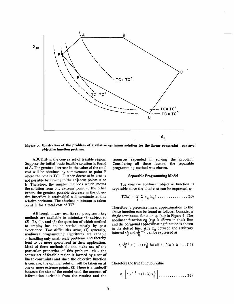
points of the convex set, indicating the possibility of the existence of multiple optima (Figure 2). Although the fact remains that the global minimum occurs at an extreme point, it is difficult to make use of this property in practice to determine th~ global extremum. If there happens
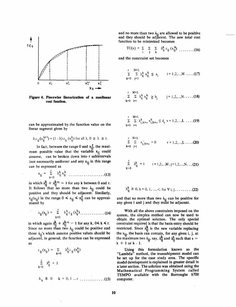
to be a relative minimum at an extreme point different from the global, such that the function value at adjacent extreme points to this relative minimum is greater, then the procedure like simplex method will terminate. Such a situation is shown in Figure 3.
Xlhf 12
XI. 12
, "
A
,If' , , .... \ v' ..... ,
B
\~, ' " ....... , C ---F I '........ ........ ..... , ..... -I .......... ..... _
I ...... ....._- -- - TC-TC2 I ...... -- -- -............ --_ I
---~------ ---TC=TC : E I -------.9 TC = TCo (Minimum) I I I I
XII. II XI. II
Figure 2. Illustration of global minimum and multiple optima for linear constraint concave objective function example.
8
\ A
I , ' \ F \ \ \ \ \ \ \ \ \ \
\ \ \ ',E , , , ,
\ \ \ \
\ \ , , , , , ,
, " , " " , ", ',TC=TC 2
" " " ..... ,
B
C , " 'TC = TC 3
............. ..... ..... ...... '"'
...... _- --- -- TC= TCI ---- --- TC = TCO
o
Figure 3. Illustration of the problem of a relative optimum solution for the Unear constraint-concave objective function problem.
ABCDEF is the convex set of feasible region. Suppose the initial basic feasible solution is found at A. The greatest decrease in the value of the total cost will be obtained by a movement to point F where the cost is Tel. Further decrease in cost is not possible by moving to the adjacent points A or E. Therefore, the simplex methods which moves the solution from one extreme point to the other (where the greatest possible decrease in the objective functiion is attainable) will terminate at this relative optimum. The absolute minimum is taken on at D for a total cost of TCo.
Although many nonlinear programming methods are available to minimize (7) subject to (2), (3), (4), and (5) the question of which method to employ has to be settled mostly by past experience. Two difficulties arise, (1) generally, nonlinear programming algorithms are capable of handling only small-scale problems and thereby tend to be more specialized in their application. Most of these methods do not make use of the particular properties of this problem, viz., the convex set of feasible region is formed by a set of linear constraints and since the objective function is concave, the optimal solution will be taken on at one or more extreme points. (2) There is a tradeoff between the size of the model (and the amount of information derivable from the results) and the
9
resources expended in solving the problem. Considering all these factors, the separable programming method was chosen.
Separable Programming Model
The concave nonlinear objective function is separable since the total cost can be expressed as
TC(x) = ~ ~ cij (xij ) ................ (10) t J
Therefore, a piecewise linear approximation to the above function can be found as follows. Consider a single continuous function cij (Xij) in Figure 4. The nonlinear function Cij (xij) IS snown in thick line and the polygonal approximating function is shown in the dotted line. Any Xij between the arbitrary interval xb and x~ + 1 can be expressed as
A x~+ 1 + (1 - A) x:',c for all A, 0 ~ A ~ 1 ... (11) IJ IJ
Therefore the true function value
c.. A x.. + (1 - A) x .. [ k+l kJ IJ IJ IJ ••••••••••••••• (12)
Tell
XIJ~
Figure 4. Piecewise linearization of a nonUnear cost funtlon.
can be approximated by the function value on the linear segment given by
AC .. (X.~+l) + (1 - A) COO (x~) for all A, ° 2: A ~ 1. IJ IJ IJ IJ
In fact, between the range 0 and xij, the maximum possible value ,that the variable Xij could assume, can be broken down into r subintervals (not necessarily uniform) and any Xij in this range can be expressed as
r k k xij = L Aij xij ................... (13)
k=O
in which Alj + .>,;+1 = 1 for any k between 0 and r. It follows that no more than two ~j could be positive and they should be adjacent. Similarly, c··(x··) in the range 0 ~ x·, ~ x'- can be approxi-lj lj 1J lj mated by
C .. (x .. ) = ~ A~C .. (x~) (14) IJ IJ IJ IJ IJ·············
k=O
in which again Af. + Alj+l = 1 for any k, O~ k ~ r. Since no more t~an two .>,j could be positive and those .>,j'S which assume positive values should be adjacent. in general, the function can be expressed as
Coo (x .. ) = L A~Coo (x~) IJ IJ k=O 1J IJ IJ
r L A~ = 1
k=O
A k ~ ° k = 0, 1 ... r ............. (15)
10
and no more than two ~j are allowed to be positive and they should be adjacent. The new total cost function to be minimized becomes
TC(x) = L L L A~ COO (x.~ (16) i j k IJ IJ 1) ..••••.• .
and the constraint set becomes
i= 1,2, ... ,M .... (17)
r M+L
L .L ~~Xi~ ~~ bj k=O Fl
j = 1 ,2, ... ,N ..... (18)
r M+L L L A~N+ x~N+ :::; dy v = 1,2, ... ,L .... (19)
1, y 1, y-
k=O i=l
r N+L L L
k=O j=l X.'N+ = ° 1, Y
v = 1 ,2, ... ,L .... (20)
r L A~. = 1
k=O IJ i = 1 ,2, ... ,M ;j= 1,2, ... ,N ... (21)
A~ 2: 0, k = 0, 1, ... , r; for Vi, j ......... (22)
and that no more than two \i can be positive for any given i and j and they must be adjacent.
With all the above constraints imposed on the system, the simplex method can now be used to obtain the optimal solution. The only special constraint required is that the basis entry should be restricted. Since \~ is the new variable replacing the Xij' the basis can contain, for any given i, j, at the maximum two '>'j' say, .>,~ and ~j such that s = k + 1 or k - 1.
Using this formulation known as the "Lambda" method, the transshipment model can be set up for the case study area. The specific model development is explained in greater detail in a later section. The solution was obtained using the Mathematical Programming System called TEMPO available with the Burroughs 6700 computer.

Seasonal variations In the model parameters
In the initial model, the solutions were obtained for the case study area with annual flows. It was assumed that the flow rate was constant at all points in time throughout the year. In reality, extensive variations in the flow rates of surface water and in the quantity of water required for various purposes vary with seasons, time of year, even to the time of day. Particularly for this analysis, seasonal changes affect the system results considerably and, therefore, the water budgeting procedure was carried out for each season and the water availabilities and quantities required were estimated. With these values, the transshipment model was solved to appraise the system operation over seasons of a year and over future years.
Stochastic Considerations
In a general programming model of the form,
Min Z = f(x) _ ............ (23) Subject to g (x) ~ b
x ;:: 0 ............ (24)
(1) The parameters of the objective function f (X), (2) the parameters of the constraint equations g(f) and (3) the right-hand-side elements of b can be random. For the transportation model under! consideration, all the coefficients ofg(X) are 0, 1, or : -1, and they are fixed. Therefore, randomness can i
be found only in the_cost function parameters] (x) and the elements of b . It will be assumed that the cost coefficients are determin~tic and only the , randomness in the elements of b will be treated.
Suppose the kth constraint
(-) < b gk x - k.··· ................... (25)
is desired to hold with at least a probability of 95 percent, when bk is assumed to be a normal random variate. This can be written as
Pr [gk (x) :s bk ] 2: ~k ........... (26)
in which ~k = 0.95
Subtracting E(bk) where E denotes expectation operator, from both sides of the inequality within
11
the square brackets and dividing by Obk' the standard deviation ofbk, we have
[
g k (x) - E (bk ) bk - E(bk)] Pr :s 2: f\
abk
a bk ..• (27)
bk
- E(bk
) The quantity Z = is a standard normal a
bk -
variate rv N (0, O. If the probability density function of Z is 'I'(Z) , then
1./;-1 (~ ) = kf./ ..................•.. (28) k "'k
which can be obtained from a table of distribution of standard, normal, random variables. Equation (27) can be true if and only if
gk (x) - E(bk )
or
gk (x):S E(b k) + kt\ abk
............ (29)
Equation 29 is a deterministic linear constraint if gk (x) is linear and assures that the kth constraint will hold with 95 percent probability. This approach is known as the chance-constrained programming and was originally developed by Charnes and Cooper (1963). Using this method, the stochasticity in the random right-hand-side elements will be accounted for.
Summary of Model Runs for the Case Study Area
The various structural changes in the basic transportation model described above were used in a number of different combinations as shown in Table 1. For each of these combinations, optimal solutions were obtained for the target years of 1975, 1980, 1985, 2000, and 2020 in order to determine the effects of each set of modifications. The results of this analysis are presented in Chapter IV.

Table 1. Summary of model runs under various model structures.
Cost Function Spatial Time Period Treatment Demand/Supply Resolution Level Ch~rac teristics
0 0
rn lO Co)
C ~~ :::l C >0"1 rn
I-< 0 0 c ~~ 'S ,~ ro 'On 'On ";! ro '§ +"'
I-<~ rn Cl) Cl) Cl) ";! "t:l eu I-< ,S I-< I-< t::: t::: Cl)
""' ..c:: Run Combinations ro ..D ..D ::s 0 -Eb~ .s Cl) "2 ::s ::s t::: rn 0 g
t::: 0 CI) CI)
~ ro Co)
ttl Cl) .....
~ Cl) (1) ~ 0 Z r-!. M 00 (/.) C7.)
Phase I 1 x x x x x
2 x x x x x
3 x x x x x
4 x x x x x
5 x x x x x
6 x x x x x
7 x x x x x
8 x x x x x
12

CHAPTER III
WATER RESOURCES AVAILABILITY, WATER REQUIREMENTS, AND WATER REUSE COSTS
Water supply in the study area can be drawn from various available sources. Surface water is drawn from the Jordan River and the Wasatch Front streams and their associated storages; imported water through various canals and aqueducts; and groundwater through a system of wells and springs. Municipal and industrial effluents are included as alternative water supply sources through water reuse.
In addition to annual study, the water availability and water requirements were arbitrarilly divided into two seasons, namely, the winter season, lasting between the month of October till the month of March, and the summer season, commencing in April and ending in September. The summer season approximately corresponds to the irrigation period in the area.
Surface Streams Water
There exists two major sources of surface stream water sources: The Jordan River and the Wasatch Front streams. The Oquirrh Mountains streams are generally ephemeral streams with insufficient flow to be developed economically into reliable supply sources. Table 2 shows the long-term annual and seasonal means of the Jordan River at the stations near the Narrows, and the Wasatch Front str(~ams-the Big Cottonwood Creek, the Little Cottonwood Creek, Mill Creek, Parley Creek, Emigration Creek, City Creek, and Red Butte Creek. The 9S percent supply availability by norma] deviation assumption and by I
rank for seasonal flow is also included in Table 2. Zero flow was substituted where the computation of flow was negative, since negative flow is physically impossible.
Jordan River
The Jordan River is the single largest surface water source in the study area. The long-term average annual flow, over a S8 year period, of the river entering the Salt Lake County at the Narrows
is almost 260,000 acre-feet which is more than the total combined flow of the Wasatch Front streams. The Jordan River water has been largely diverted for irrigation purposes while a small amount has been diverted for industrial consumption.
The Wasatcb Front streams
The Wasatch Front streams which are the major tributaries of the Jordan River in the study area, are the Big Cottonwood Creek, Little Cottonwood ~reek in subarea F2, Mill Creek in subarea G, Parley Creek, City Creek, Emigration Creek, and Red Butte Creek in subarea E. The total combined flow available from these creeks is approximately 142,000 acre-feet annually. Most streams were well developed as sources of supply in the study area, including the construction of a number of reservoirs and diversion canals.
Groundwater
Groundwater in the study area is obtained through well pumping and free flowing springs. The amount of groundwater utilization in the area has been increasing. In the past decade, the average groundwater utilization was well over 100,000 acre-feet per year (Figure 5). Since the safe yield of groundwater in the area is approximately 150,000 acre-feet per year (Table 3), the groundwater use is reaching its maximum potential without possible groundwater mining. Groundwater is used for various purposes but mainly in agricultural sectors.
Imported Water
The 3' u:iy area imports a relatively small amount of water from nearby sources. The existing imports are throll.gh the Salt Lake aqueduct for municipal supply, Hlc Provo Reservoir Canal, the Utah Lake Distributing Co. Canal mainly for irrigation, and Kennocott Copper Pipeline mainly for industrial uses. In the future, an additional imported source will be available through the
13
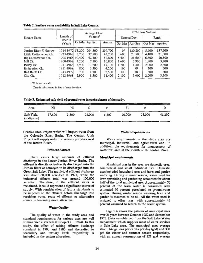
Table 2. Surface water availabllity in Salt Lake County.
Average Flow 95% Flow Volume
Stream Name Length of Volumea Normal Dev. Rank
Record (Year) Oct-Mar Apr-Sep Annual Oct-Mar Apr-Sep Oct-Mar Apr-Sep
Jordan River @ Narrow 1914-1972 55,200 204,500 259,700 Ob 120,200 5,600 137,600 tittle Cottonwood Ck. 1923-1968 5,700 37,500 43,200 3,600 23,500 4,400 21,600 Big Cottonwood Ck. 1905-1968 10,400 42,400 52,800 5,400 21,600 6,600 20,500 Mill Ck. 1900-1968 3,200 7,500 10,800 1,600 2,900 1,900 3,700 Parley Ck. 1911-1968 3,900 13,200 17,100 1,700 1,300 2,000 2,800 Emigration Ck. 1911-1968 800 3,300 4,200 100 Ob 200 600 Red Butte Ck. 1943-1972 700 1,700 2,500 300 300 300 300 City Ck. 1912-1968 2,900 8,500 11,400 2,100 3,600 2,000 3,700
aVolume in ac-ft.
bZero is substituted in lieu of negative flow.
Table 3. Estimated safe yield of groundwater in each subarea of the study.
Area
Safe Yield (ac-ft/year)
HI
17,800
H2 G
3,500 28,000
Central Utah Project which will import water from the Colorado River Basin. The Central Utah Project will supply water for various purposes west of the Jordan River.
Emuent Sources
There exists large amounts of effluent discharge in the Lower Jordan River Basin. The effluent is directly or indirectly discharged into the Jordan River or conveyed to be discharged into the Great Salt Lake. The municipal effluent discharge was about 80,000 acre-feet in 1971, while the industrial effluent total was around 100,000 acre-feet. Therefore, if the effluent water is reclaimed, it could represent a significant source of supply. With consideration of future standards to be imposed on the effluent before discharge into receiving water, reuse of effluent as alternative source is becoming more attractive.
Water QuaUty
The quality of water in the study area and standard requirements for various uses are well summarized elsewhere (Bishop et al., 1974). In this study, the effect of raising effluent discharge standard in 1980 and 1985 and thereafter to secondary and tertiary levels respectively is included in the system allocation.
14
Fl F2 E D
6,500 20,000 28,000 46,200
Water Requirements
Water requirements in the study area are municipal, industrial, and agricultural and, in addition, the requirements for management of waterfowl area at the mouth of the Jordan River.
Municipal requirements
Municipal uses in the area are domestic uses, commercial and small industrial uses. Domestic uses included household uses and lawn and garden watering. During summer season, water used for lawn sprinkling and gardening accounted for about half of the total municipal use. Approximately 70 percent of the lawn water is consumed with estimated 30 percent percolated to groundwater system. During winter season watering lawn and garden is assumed to be nil. All the water used is assigned to other uses, with approximately 4S percent assumed to return to the sewer system.
Figure 6 shows the pattern of municipal uses over 21 years between October 1952 and September 1973. Data was obtained from the Salt Lake Water Department which supplies most of water services in Sale Lake area. The municipal uses average about 142 gallons per capita per day (gcd) and 300 gcd for winter and summer season respectively, with an annual consumption of 221 gcd average
...: -I 120 cj 0
"0 c: fi :J 0
E I/O z ~ cr 0 I I-§ 100
cr lLJ
~ ~ 0 90 z => 0 Q: (!)
1960 1962 1964 1966 1968
YEAR'
Figure 5. Groundwater withdraw for aU purposes in Salt Lake County (1960-1968).
(compared with 224 gcd used in a previous report (Bishop et al., 1974». Analysis of data did not indicate any significant trend in water uses, therefore it is assumed that uses are constant throughout the study. Table 4 shows the mean and 9S percent normal deviation water requirements in the study area for the winter and summer seasons and the annual.
Table 4. Municipal water .... In Salt Lake City serviced by Salt Lake City Water D.,artment during the period October 1952-September 1973.
Periods Winter Summer Annual
Mean (gcd) 142 300 221
95% Normal Deviate 115 248
Variation of uses during summertime could well be explained in terms of precipitation availability. The major municipal use during summer is lawn and garden watering, and in wet
15
summers water use was relatively low while in dry summers water use was relatively high.
Industrial uses
The industrial uses in the area are assumed to be approximately constant throughout the year. The industrial uses are also assumed to be relatively constant throughout the period of study with the exception of subarea E, containing Salt Lake City, in which small amounts of increases industrial uses are expected.
Agricultural uses
The main agricultural use is irrigation. Domestic stock is the second major use. Irrigation in the study area occurs largely between April and October. The amount of irrigation water used in October is relatively small; therefore, it is assumed that all the requirement for irrigation occurs between April and October. It is further assumed that irrigation use reflects total use in the agriculture sector. Losses due to seepage in canals
20
-.E
c .2 - 10 0 -:9-u G) '-0..
350
300
-c u t!)
c o -0. E ::J en c o u
200
~ ~ ~ I, \ 1\ A / \
\ " '\ " '~ .. ~ \ , I t:\, \ ~ ~'~, \
~--<!)--&- ' \ .J \ Annual 'ts>-.. \
cb
at SLC Airport
100L-----------~~--------~--~----~~--------~~~~ ItlS 1960 1965
Water Year
Figure 6. Comparison of munlcipal water' consumption and IJ.lpltatio~.
16
and delivery systems are assumed to be 15 percent of diversion. Of the total field delivery, about 10 percent is assumed to return to surface water sources, about 30 percent goes to groundwater, and the rest is consumed (Hely et aI., 1970).
To compute the 95 percent level of agricultural use, certain assumptions about crops and climatic conditions have to be made. In light of reducing acreage of crop land, it is expected that in the future cash crops will be more attractive. However, it is safe to assume that certain crops which require larger amounts of irrigated water are goint to be planted. Alfalfa and sugar beets are assumed to be the selected crops. Both crops require approximately the same amount of irrigation water over the season. The 95 percent requirement is then computed from monthly moisture requirement of the crop given that the natural available precipitation and temperature are 95 percent of average. Irrigation practices are assumed to have varied efficiency. The diversion requirement for each level of irrigation efficiency is shown in Table 5.
Table 5. Irrigation diversion requirement at 95 percent level.
Consumptive in/acre 35.03
30 116.8
Efficiency 50 70.1
HISTORICAL
en 0::
2000
I~ ·I~
70 50.0
Water Reuse Costs
The cost matrix forms the basis for decisionmaking in the linear programming transportation model. The literature was reviewed to determine the appropriate cost functions for each method of waste treatment and water reuse, and for water and wastewater transportation. The construction costs were then ajusted to June 1974 by the use of the ENR Building Cost Index. The operation and maintenance (O&M) costs are adjusted by the use ofthe labor rates for sanitation workers, published by the Bureau of Labor Statistics. The water transportation costs were adjusted by the use of the EPA sewer construction cost index (Figure 7 and Table 6). The annual cost of the capital investment was based on 5112 percent for 30 years with a capital recovery factor (CRF) of 0.069.
A summary of the cost equations for the total cost of water treatment and reuse is presented in Table 7. The breakdown of each equation into its component cost equations is presented in Table 8, and is discussed in detai1 in Appendix A. The costs were represented by the equation, y = KXa, where y is the total dollars ($) to supply a given quantity of water, K is th,e cost coefficient, X is the quantity of water in acre-ft (AF), and a is the economy of scale factor. The values represent the costs of collecting the water from a source or from the effluent of a treatment process, and transporting the water to a destination for use or for treatment to the quality
. PROJECTED
~I 20
. L&J al ~ :J Z
1600 ENR BUILDING COST INDEX 1949= 100
16 0:: :c "'.q)o
X L&J o Z
CD I
0:: Z L&J
d5 en
I
U a.. ~
1200
800
400
o 1960 1970 1980
Figure 7. Comparison of cost indices.
1990 2000 2010 2020
YEAR
17
12
8
4
o 2030
en L&J I« a::: a::: o CD « ...J
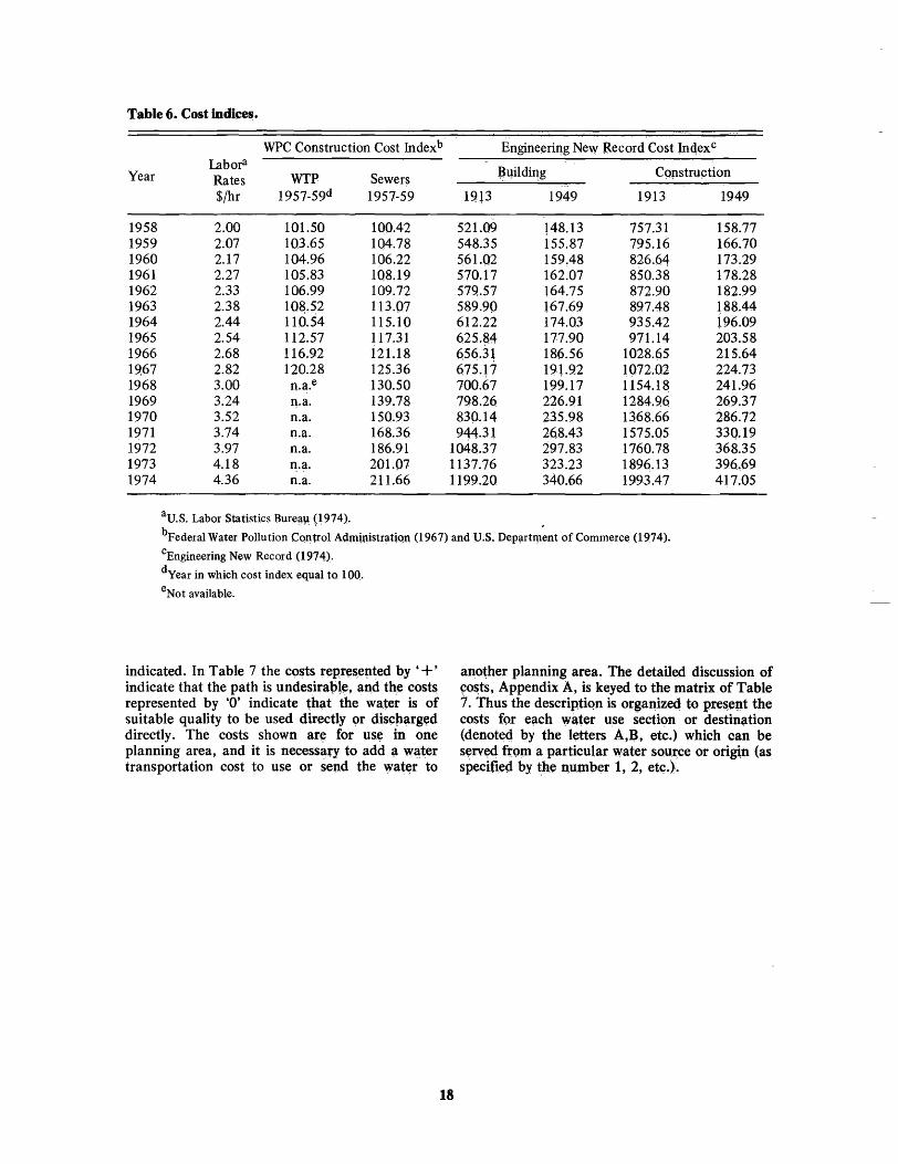
Table 6. Cost indi~.
WPC Construction Cost Indexb Engineering New Record Cost lnqexC
Lab ora ~llilding CQP.stru~tion Year Rates WTP Sewers
$/hr 1957-59d 1957-59 1913 1949 1913 1949
1958 2.00 101.50 100.42 521.09 148.13 757.31 158.77 1959 2.07 103.65 104.78 548.35 155.87 795.16 166.70 1960 2.17 104.96 106.22 561.Q2 159.48 826.64 173.29 1961 2.27 105.83 108.19 570.17 162.07 850.38 178.28 1962 2.33 106.99 109.72 579.57 164.75 872.90 182.99 1963 2.38 108.52 113.07 589.90 167.69 897.48 188.44 1964 2.44 110.54 115.10 612.22 174.03 935.42 i96.09 1965 2.54 112.57 117.31 625.84 177.90 971.14 203.58 1966 2.68 116.92 121.18 656.31 186.56 1028.65 215.64 19,67 2.82 120.28 125.36 675.l7 19l.92 1072.02 224.73 1968 3.00 n.a.e 130.50 700.67 199.17 1154.18 241.96 1969 3.24 n.a. 139.78 798.26 226.91 1284.96 269.37 1970 3.52 n.a. 150.93 830.14 235.98 1368.66 286.72 1971 3.74 n.a. 168.36 944.31 268.43 1575.05 330.19 1972 3.97 n.a. 186.91 1048.37 297.83 1760.78 368.35 1973 4.18 n.a. 201.07 1137.76 323.23 1896.13 396~69 1974 4.36 n.a. 211.66 1199.20 340.66 1993.47 417.05
aU.S. Labor Statistics Bure~~ (1974).
bpederal Water Pollution Control AdIIli!,listratjOl1 (1967) and U.S. Dep~rtIIl~nt of CommerCe (1974).
CEngineering New Record (1974).
dYear in which cost index equal to 10Q.
eNot available.
indicated. In Table 7 the costs repre~e~ted by '+' indicate that the path is undesirap~e, a~d the costs represented by '0' indicate that the water is of suitable quality to be used directly or discpargt;d directly. The costs shown ar~ for USt; in one planning area, and it is necessary t9 add a w3:ter transportation cost to use or send the 'Yater to
18
ano~her planning area. The detailed discussion of 4:0&ts, Appendix A, is keyed to the matrix of Table 7. Thus the descripti()D is orgallized to pre~eI,lt the costs for e~ch ':Vat~r use section or destination (denoteci by the letters A,B, etc.) which can be served ft()J:ll a particular water source or origi,n (as specified by t,he number 1, 2, et~.).

""'" 100
Table 7. Total water treatment and reuse cost equationa, y = KXa.
- -- -- -- --- -- - ----- ----- -- --- -- -
Destinations A B C D E F G H I J K
Water Municipal Industrial Agricultural
Existing Wastewater Wastewater Wastewater Wastewater Water System Treatment Culinary Secondary Treatment Treatment Treatment Treatment Fowl
Origins Plants Water Water Water Treatment Levell Level 2 Level 3 For Reuse Outflow Outflow
1 Surface Water Better 243 XO.773 829 XO. 779 725 XO.S9S 4747 XO. 31 + + + + + 0 0 Than Class C
2 Water Treatment + 81.0 XO.9O 81.0 XO.9O 81.0 XO.9O
Plant + + + + + + +
3 Wells 496 XO. 714 245 XO.842 206 XO. 768 199 XO.7S + + + + + + +
4 Municipal Effluent + + + + 430 ~.8S3 556 XO.847 807 XO.821 1387 XO. 79O 1620~·802 + +
5 Industrial Effluent + + + + 459 ~.848 583 xO·844 836 X°.819 1419 ~.789 1662~·800 + +
6 Existing Secondary
4747 XO.31 481 1'.644 1254 XO.674 1199 ~.7S4 0 0 Treatment + + + + +
7 Wastewater Treat-
4747 ~.31 505 XO.644 1317~·674 1259 XO. 7S4 0 0 ment Levell + + + + +
8 Wastewater Treat-
1124 XO.S1 4747 XO.31 834 XO.686 891 XO. 774 0 0 ment Level 2 + + + + +
9 Wastewater Treat-
873 XO. 706 1124Xo.S1 4747 XO.31 275 ~.841 0 0 ment Level 3 + + + + +
10 Wastewater Treat-
81.0 XO.9O 1124 XO.S1 4747 XO.31 0 0 ment for Reuse + + + + + +
11 Surface Water Worse
216 XO.839 782 XO.S03 322 XO.767 4747 ~.31 0 0 Than Class C + + + + +
12 CUP Jordan
124 XO.962 289 XO.866 289 XO.866 Narrows WTP + + + + + + + +
- - '-----
aCost equations represent total cost in June, 1974, dollars ($) with X in AF/YR. The + symbol indicates an undesirable use, and was given the value y = 9999 X1
.O
. The 0 symbol indicates a zero (0) cost. Costs are given to go from effluent of origin to effluent of destination.
J
J
I
I
I

Table 8. Summary of cost equationa•
~ b c Destination Eq Unit Processes Capital O&M Total
ORIGIN 1: Surface Water Better Than Class C
Water handling 10.3 Xo. 90. 24.1 Xo.·90. 34.5 XO.9O
Water Water collection from river
A Treatment 2 Water treatment plant 81.0 XO. 67 245 XO.67 326 XO.67
Plants Existing
3 Composite cost equation 243 XO.773
5 Water handling 44.6 XO.9 0. 70.8 XO.9.O 115 XO.90. Water collection from river
Municipal Water distribution B Culinary 6 Water treatment plant 256 XO.69.2 770 Xo.·692 1026 XO.692
Water New
7 Composite cost equation 829 )f.779
10 Water handling 282 XO.S36 475 XO.613 725 Xo.·S9S
C Industrial Pumpage from river
Water Chlorination
11 CompOSite cost equation 725 Xo.·S9S
14 Water handling 2768 X 0..32 1972 Xo.·29S 4747 Xo.·31
Agricul tural Diversion struc tures D Water Canal costs
15 Composite cost equation 4747 XO,31
ORIGIN 2: Water Treatment Plants
Municipal 4 Water handling 34.3 XO•90. 46.7 XO.90. 81.0 Xo.·90.
B Culinary Water distribution
Water 16 Composite cost equation 81.0 Xo.·9O
Industrial 4 Water handling 34.3 XO.90. 46.7 Xo.·90. 81.0 XO.90. C Water Water distribution
17 Composite cost equation 81.0 Xo.·9O
Agricultural 4 Water handling 34.3 XO.9O 46.7 XO.9O 81.0 XO·9O
D Water Water distribution
18 Composite cost equation 81.0 XO.9O
ORIGIN 3: Wells
19 Water handling 818X°.4S3 33.2 XO.90. 199 XO. 7S
Water Well water A Treatment 2 Water treatment plant 81.0 XO.67 245 XO.67 326 Xo.·67
Plants Existing
20 Composite cost equation 496 Xo.·714
21 Water handling 206 XO.753 89.1 Xo.·9O 245 Xo.·842
Municipal Well water
B Culinary Chlorination
Water Water distribution
22 Composite cost equation 245 )f.842
20
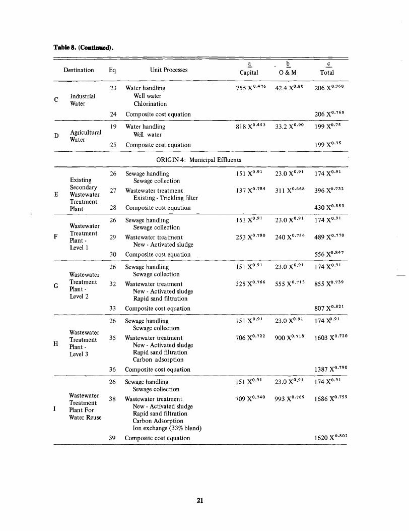
Table 8. (Contlnaecl).
!. b c Destination Eq Unit Processes -
Capital O&M Total
23 Water handling 755 X°.476 42.4 XO.8O 206 XO.768
C Industrial Well water Water Chlorination
24 Composite cost equation 206 XO.768
19 Water handling 818 X°.453 33.2 XO.9O 199 XO. 75
D Agricul tural Well water Water
25 Composite cost equation 199 XO.7S
ORIGIN 4: Municipal Effluents
26 Sewage handling 151 XO.91 23.0 XO.91 174 XO.91
Existing Sewage collection Secondary 27 Wastewater treatment 137 XO. 784 311 XO.668 396 XO.732
E Wastewater Existing - Trickling filter Treatment Plant 28 Composite cost equation 430 XO.853
26 Sewage handling 151 XO.91 23.0 XO.91 174 XO.91
Wastewater Sewage collection
F Treatment 29 Wastewater treatment 25? XO. 78O 240 XO. 756 489 XO. 77O
Plant -Levell New - Activated sludge
30 Composite cost equation 556 XO.847
26 Sewage handling 151 XO. 91 23.0 XO.91 174 XO.91
Wastewater Sewage collection
G Treatment 32 Wastewater treatment 325 XO. 766 555 XO.713 855 XO.739
Plant - New - Activated sludge Level 2 Rapid sand filtration
33 Composite cost equation 807 XO.821
26 Sewage handling 151 XO.91 23.0 XO.91 174 -X>.91
Wastewater Sewage collection
Treatment 35 Wastewater treatment 706 XO. 722 900 XO. 718 1603 XO.72O
H Plant - New - Activated sludge
Level 3 Rapid sand filtration Carbon adsorption
36 Composite cost equation 1387 XO.79O
26 Sewage handling 151 XO.91 23.0 XO.91 174 XO.91
Sewage collection Wastewater
38 Wastewater treatment 709 XO.74O 993 XO. 769 1686 XO.759
Treatment Plant For
New - Activated sludge
Water Reuse Rapid sand filtration Carbon Adsorption Ion exchange (33% blend)
39 Composite cost equation 1620 XO.802
21
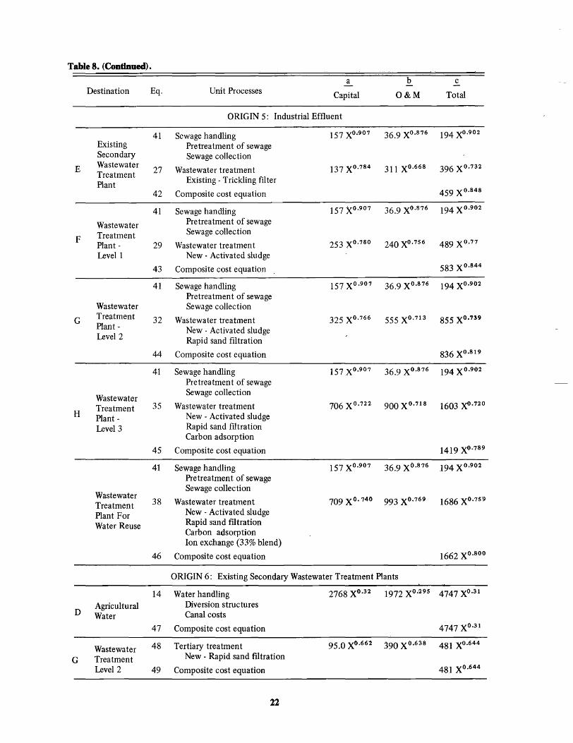
Table 8. (Continued).
a b c Destination Eq. Unit Processes Capital O&M Total
ORIGIN 5: Industrial Effluent
41 Sewage handling 157 XO;907 36.9 XO.876 194 XO.902
Existing Pretreatment of sewage Secondary Sewage collection
E Wastewater 27 Wastewater treatment 137 XO.784 311 XO.668 396 XO.732
Treatment Plant
Existing - Trickling ftl ter
42 Composite cost equation 459 XO.848
41 Sewage handling 157 XO.907 36.9 XO. 876 194 XO.902
Wastewater Pretreatment of sewage
F Treatment Sewage collection
Plant - 29 Wastewater treatment 253 XO. 78O 240 XO.756 489 XO. 77
Levell New - Activated sludge
43 Composite cost equation 583 XO.844
41 Sewage handling 157 XO.907 36.9 XO.876 194 XO.902
Pretreatment of sewage Wastewater Sewage collection
G Treatment 32 Wastewater treatment 325 XO. 766 555 XO. 713 855 XO.739
Plant -Level 2
New - Activated sludge Rapid sand ftltration
44 Composite cost equation 836 XO.819
41 Sewage handling 157 XO.907 36.9 XO.876 194 XO.902
Pretreatment of sewage
Wastewater Sewage collection
Treatment 35 Wastewater treatment 706 XO. 722 900 XO.718 1603 Xo.no H Plant - New - Activated sludge
Level 3 Rapid sand filtration Carbon adsorption
45 Composite cost equation 1419 XO.789
41 Sewage handling 157 XO.907 36.9 XO.876 194 XO.902
Pretreatment of sewage
Wastewater Sewage collection
Treatment 38 Wastewater treatment 709 X O• 740 993 XO.769 1686 XO.759
Plant For New - Activated sludge
Water Reuse Rapid sand ftltration Carbon adsorption Ion exchange (33% blend)
46 Composite cost equation 1662 XO.8OO
ORIGIN 6: Existing Secondary Wastewater Treatment Plants
14 Water handling 2768 XO.32 1972 XO.295 4747 XO.31
D Agricultural Diversion structures Water Canal costs
47 Composite cost equation 4747 XO.31
Wastewater 48 Tertiary treatment 95.0 XO.662 390 XO.638 481 XO.644
G Treatment New - Rapid sand fIltration
Level 2 49 Composite cost equation 481 XO.644
22

Table 8. (ContIDaed).
~ b .£ Destination Eq Unit Processes Capital O&M Total
Wastewater 50 Tertiary treatment 607 XO.633 694 XO.694 1254 XO.674
H Treatment New - Rapid sand filtration
Level 3 Carbon adsorption
51 Composite cost equation 1254 XO.674
52 Tertiary treatment 502 XO.698 753 XO.733 1199 XO.7S4
Wastewater New - Rapid sand fIltration Treatment Carbon adsorption For Water Ion exchange (33% blend) Reuse
53 Composite cost equation 1199 XO.7S4
ORIGIN 7: Wastewater Treatment - Levell
14 Water handling 2768 XO.32 1972 XO.29S 4747 XO.31
Agricultural Diversion structures D Water Canal costs
54 Composite cost equation 4747 XO.31
Wastewater 55 Tertiary treatment addition 99.8 XO.662 410 XO.638 505 XO.644
G Treatment New - Rapid sand filtration
Level 2 56 Composite cost equation 505 XO.644
Wastewater 58 Tertiary treatment addition 637 XO.633 729 XO.694 1317 XO.674
H Treatment New - Rapid sand fIltration
Level 3 Carbon adsorption
59 Composite cost equation 1317 X 0.674
61 Tertiary treatment addition 527 XO.698 791 XO. 773 1259 XO.7S4
Wastewater New - Rapid sand filtration Treatment Carbon adsorption For Water Ion exchange Reuse
62 Composite cost equation 1259 XO. 7S4
ORIGIN 8: Wastewater Treatment - Level 2
Industrial 8 Water handling 292 XO.S1 832 XO.S1 1124 XO.S1
C Water Water pumping
63 Composite cost equation 1124 XO.S1
14 Water handling 2768 XO.32 1972 XO.29S 4747 XO.31
D Agricultural Diversion structures Water Canal costs
64 Composite cost equation 4747 XO.31
Wastewater 57 Tertiary treatment addition 541 XO.626 366 XO.724 834 XO.686
H Treatment New - Carbon adsorption
Level 3 65 Composite cost equation 834 XO.686
Wastewater 66 Tertiary treatment addition 434 :X<>.703 526 XO.799 891 XO. 774
Treatment New - Carbon adsorption
For Water Ion exchange (33% blend)
Reuse 67 Composite cost equation 891 XO.774
23

Table 8. (Continued).
Destination Eq Unit Processes .! b .£ Capital O&M Total
ORIGIN 9: Wastewater Treatment - Level 3
Water 70 Wa ter handling 1544 XO.535 179 XO.822 873 XO.706
A Treatment Water transmission
Plants 71 Composite cost equation 873 XO.706
8 Water handling 292 XO.51 832 XO.51 1124 XO.51
C Industrial Water pumping Water
72 Composite cost equation 1124 XO.51
14 Water handling 2768 XO.32 1972 XO.295 4747 XO.31
D Agricultural Diversion structures Water Canal costs
73 Composite cost equation 4747 XO.31
74 Tertiary treatment addition 44.8 XO. 841 230 XO. 841 275 XO. 841
Wastewater New - Ion exchange Treatment (33% blend) For Water Reuse 75 'Composite cost equation 275 XO.841
ORIGIN 10: Wastewater Treatment - For Water Reuse
4 Water handling 34.3 XO.9O 46.7 XO.9O 81.0 XO·9O
Municipal Water distribution B Culinary
Water 76 Composite cost equation 81.0 XO.9O
Industrial 8 Water handling 292 XO.51 832 XO.51 1124 XO.51
C Water Water pumping
77 Composite cost equation 1124 XO.51
14 Water handling 2768 XO.32 1972 XO.295 4747 XO.31
Agricul tural Diversion structure D
Water Canal costs
78 Composite cost equation 4747 XO.31
ORIGIN 11: Surface Water Worse Than Class C
80 Water handling 2004 XO.9O 41.0 XO.941 60.9 XO.93O
Water collection from river Water Water pretreatment
A Treatment 2 Water treatment plant 81.0 XO.67 245 XO.67 326 XO.67
Plant Existing
81 Composite cost equation 216 XO.839
82 Water handling 54.8 XO.9O 86.3 XO.923 141 XO.915
Water collection from river
Municipal Water pretreatment Water distribution
B Culinary 256 XO.692 770 XO.692 1026 XO.692
Water 6 Water treatment plant New
83 Composite cost equation 782 XO.803
24

Table 8. (Continued).
Destination Eq Unit Processes a b c -
Capital O&M Total
85 Water handling 124 XO. 708 212 XO.785 322 XO.767
Industrial Pumpage from river
C Water pretreatment Water Chlorination
86 Composite cost equation 322 XO. 767
14 Water handling 2768 XO.32 1972 XO.295 4747 XO.31
Agricultural Diversion structure D Water Canal costs
87 Composite cost equation 4747 XO.31
ORIGIN 12: Central Utah Project - Jordan Narrows Water Treatment Plant
89 Water handling 56.5 XO.966 67.6 XO.959 124 XO.962
Municipal Purchase price B Culinary Water distribution
Water 90 Composite cost equation 124 XO.962
92 Water handling 95.8 XO.9O 203 XO.838 289 XO.866
C Industrial Purchase price Water Pumping
93 CompOSite cost equation 289 XO.866
92 Water handling 95.8 XO.9O 203 XO.838 289 XO.866
D Agricultural Purchase price
Water Pumping
94 Composite cost equation 289 XO.866
aCost equations represent component costs in June 1974, dollars ($) with X in AF/YR.
25


CHAPTER IV
MODEL OPERATION AND COMPARISON OF RESULTS
Comparative Analysis of Model Runs
The basic model employed for the study can be structured with varying complexity from a simple model consisting of a grouped sectoral division of users and aggregated sources to a highly complex model incorporating finely divided users, based on spatial, temporal, and water quality aspects, and segregated sources. The larger and more complex the model, the higher the cost of solution in terms of computer time, disk storage, and the labor involved in data analysis and model structuring. But the information that can be gained may also increase because a complex model involves less of abstraction from the real world.
In this chapter a number of optimal solutions for different model structures are analyzed in order to compare the costs and the amount of relevant information each yields. The results of various model structures are discussed under the following headings:
4. Linear versus nonlinear costs
S. Deterministic versus stochastic supplies
Table 9 is constructed to indicate model runs referred to in Table 1 from which the comparisons of results are derived. The x's linked by the dotted lines in the table indicate the pairs of runs from which the comparisons are drawn.
The cOl1\parisons of results in the following sections are meant to be only illustrative examples of the types of information that can be derived from the various model structures rather than complete detailed comparisons and analyses. The discussion, however, does indicate generally what information can be gained through higher levels of detail or resolution in the models.
Analysis of Results for Model Structures
Spatial aggregation versus 1. Spatial aggregation versus disaggregation disaggregation
2. Imposition of higher wastewater treatment levels
3. Annual versus seasonal variations
The aggregated model was constructed for two purposes. The first was to reduce the computer time cost for nonlinear study; and the second was to study the feasibility of a regional wastewater
Table 9. Runs used for comparison of results for various model structures.
Comparisons
1. Spatial
2. Treatment
3. Annual/Seasonal
4. Linear/Nonlinear
S. Deter. /Stochastic
Runs (Table 1)
2 3 4 5 6 7 8
x ---------------- x
x -----------------x x -----------------x x -----------------x X ----------------------------------i{
X -----------------------------------x x -----------------x
x ----------------------------------------------------------------------x x -----------------------------------------------------------------------x
27
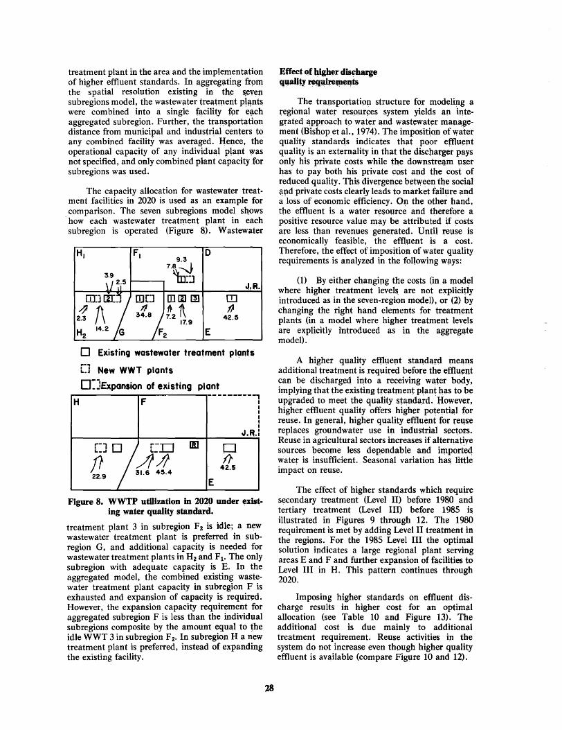
treatment pI-ant in the area and the implementation of higher effluent standards. In ~ggregating frpm the spatial resolution existing in the ~even. subregions model, the wastew~ter treatment phlnt5i were combined into a single f~cility fpr e~ch aggregated subregion. Further, the transportation distance from municipal and industrial centers to any combined facility was averaged. Hence, the operational capacity of any individu~l plapt ",as not specified, and only combined plant capacity for subregions was used.
The capacity allocation for wastewater treatment facilities in 2020 is used as an example for comparison. The seven subregions model shows how each wastewater treatment plant in each subregion is operated (Figure 8). Wastewater
HI FI 0 9.3
7.8~ 3.9 ~:] ~l ~i5 "~ft
[0] riIj [DO III 1%1 III CD ~f\ ~ 1l1\ t)
2.3 34.8/r. 7.2 17.9 42.~
H 14.2 G F E 2 2
o Existing wastewater treatment p!~nts -.. L.J New WWT plants
D:jE~pansion of existing plant
H F ----------,
I I I I I I
-I.R.:
[:J [] [:J:J [I] 0
{!.9 ! !.l1.4 ft 42.~
E
Figure 8. WWTP utUization in 2()2(j under exist-ing water quality standard.
treatment plant 3 in subregion F2 is idle; a new wastewater treatment plant is preferred in subregion G, and additional capacity is needed for wastewater treatment plants in H2 and Fl. The only subregion with adequate capacity is E. In the aggregated model, the combined existing wastewater treatment plant capacity in subregion F is exhausted and expansion of capacity is required. However, the expansion capacity requirement for aggregated subregion F is less than the individual subregions composite by the amount equaJ to the idle WWT 3 in subregion F 2. In subregion H a new treatment plant is preferred, instead of expanding the existing facility.
28
Effect Qf hlglt,r discharge q~aUty ~1J4'eQ,l~Qq "
The transportation structure for modelit}g a regional water resollr~es system yields an integrated 3;pproach to water and wastewater management (Bishop et aI., 1974). The imposition of water quality standards indicates that poor effluent quality i~ an e~ternality in that the discparger p~ys only his private costs while the downstream user has to pay both his private cost and the cost of reduced quality. This divergence between the social ~pd private costs clearly leads to market failure and a loss of economic efficiepcy. On the other hand, the effluent is a water resource and therefore a positive resource value may be attributed if ~osts a:re less than revenues generated. Until r.euse is economically feasible, the effluent is a cost. Therefore, the effect of imposition of water quality requirements is analyzed in the following w~ys:
(1) By either changing the costs (in a model where higher treatment levels are not e~plicitly introduced as in the seven-region model), or (2) by changing the right hand elements for treatment plants (in a model where higher treatment levels are explicitly introduced as in the aggreg~te model). "
A higher quality efflllent stal1dar.d qleans additional treatment is required before the efflue~t can be discharged into a receiving water body, implying that the existing treatment plant bas to be upgraded to meet the quality stapdard. 'However, higher effluent quality offers higher potential for reuse. In general, higher qllality effluent for reqse replaces groundwater use in industrial sectors. Reuse in agricultural sectors increases if alternative sources pecopte less dependable and importeq water. is insufticient. Seasonal variation ha~ l~ttle im pact on reuse.
The effect of higher stanQards which require secondary treatment (Level II) before 1980 and tertiary treatment (Level III) before 1985 is illustrated in Figures 9 through 12. The 1980 requirement is met by adding Level II treatment in the regions. For the 1985 Level III the optimal solution indicates a large regional plant serving areas E and F and further expansion of facilities to Level III in H. This pattern continues through 2020.
Imposing higher standards on effluent discharge results in higher cost for an optimal allocation (see Table 10 and Figure 13). The additional cost is due mainly to additional treatment requirement. Reuse activities in the system do not increase even though higher quality effluent is available (compare Figure 10 and 12).
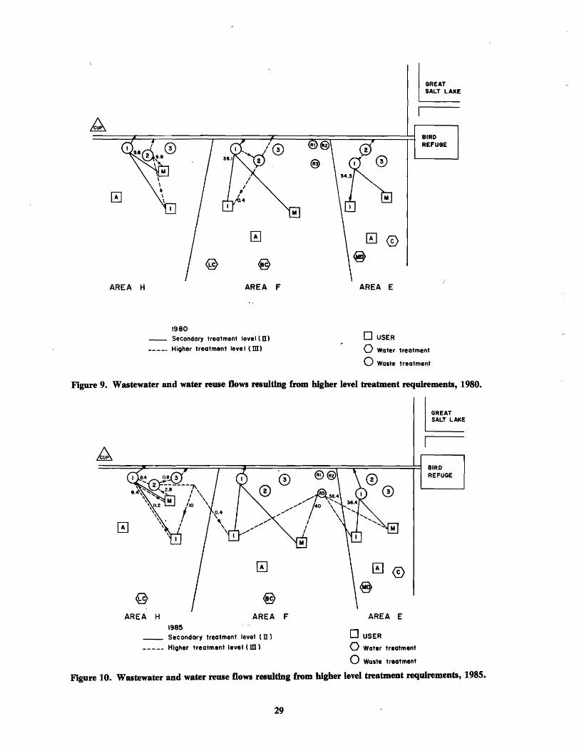
AREA H AREA F
1980 Secondary treatment level (n)
Higher treatment level (m)
AREA E
o USER
GREAT SALT LAKE
BIRD REFUGE
o Water treatment
o Waste treatment
Figure 9. Wastewater and water reuse flows resulting from higher level treatment requirements, 1980.
@
AREA H
@
AREA F 1985 Secondary treatment level (IT)
Higher treatment level (m)
AREA E
o USER
o Water treatment
o Waste treatment
GREAT SALT LAKE
BIRD REFUGE
Figure 10. Wastewater and water reuse flows resulting from higher level treatment requirements, 1985.
29
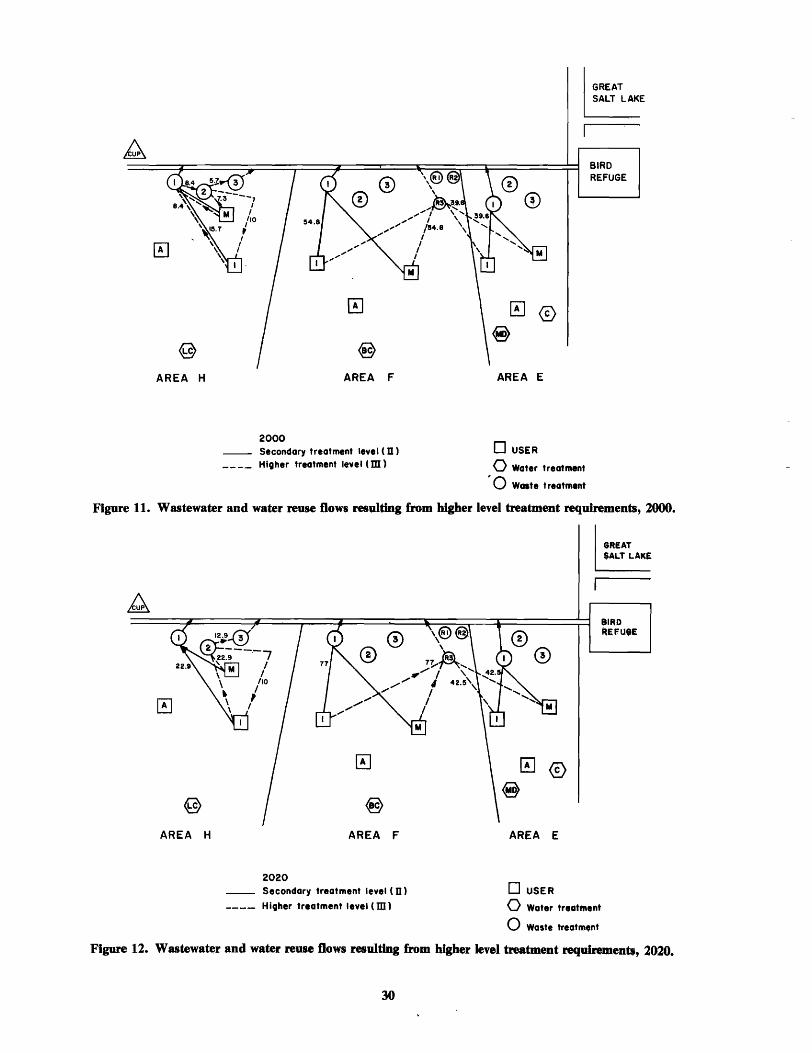
AREA H
\€D@ \ , ~39 •
........ / "', ........ I '
.... ,.... /54.8 \ .... I
AREA F
2000 Secondary treatment level (n)
Higher treatment level (m )
I I
I
®
AREA E
o USER
o Water treatment
. 0 Waste treatment
GREAT SALT LAKE
BIRD REFUGE
Figure 11. Wastewater and water reuse flows resulting from higher level treatment requirements, 2000.
AREA H AREA F
2020 Secondary treatment level ( D)
Higher treatment level (m)
AREA E
o USER
o Water treat""nt
o Waste treatment
GREAT $ALT LAKE
BIRD REFU.$E
Figure 12. Wastewater and water reuse flows resulting from higher level treatment requirements, 2020.
30

Table 10. Annual cost comparison of optimal allocations.
Allocation 1975
(a) III deterministic 13.42a
IV deterministic
(b) VII stochastic 13.57 VIII stochastic
(c) V 13.17 VI
aCost of allocation in million dollars.
28
26
24
22
.S
- 20
18
16
14
1980 1985 2000
15.09 16.47 21.00 16.25 21.32 26.31
15.13 16.54 21.06 16.23 22.00 26.76
14.42 15.62 19.28 15.60 20.07 24.20
Hio .... r tr.atm.nt ®.-: /";;'\ l.v.l, ,toc"'a,tic 1: ~ Hio ... ·r tr.atm.nt
. / /
r/
/ /
/
! l.v.l, d.t.rmini,tic
/ I® Hio .... r tr.atment .... / I.v.la - seasonal
.: / <V Secondary .: 0 stoc ... astlc - seasonal
/ ./. ® S.condar'l
/ ... tr.atm.nt
.... rr d.terministlc
/ :. ® Secondary : / treatment - seasonal / :
~ /
/
12 ~---------------~---------------~------~------------~-----------------------1~75 1980 1985 2000 2020
YEAR -..
2020
26.80 32.55
27.65 33.61
26.18 31.91
Figure 13. Comparison of total minimum. cost of optimal aUocation under various model assumptions.
31

It is recognized that the use of average annual values in the model yields estimates of capacity expansion schemes for treatment facilities in the region that may not be adequate to meet peak demand situations. The water availabilities and usage patterns fluctuate considerably over time and unless the fluctuations are taken into account, required capacities of the treatment facilities could be understated by the model. While peak demand problems were not explicitly considered in this analyses, peak factors could be applied to effluent flows to further study this aspect.
Seasonalvarlatlons
It is entirely possible that seasonal changes in supply and water requirements could substantially change allocation patterns and the total system cost. Seasonality was analyzed by solving the model for summer and winter months separately. A biseasonal year was used in order to reduce the cost of computer runs, since a finer subdivision (a monthly or a four-season model) involves considerably more computational effort. The water flow and usage in the study are~ generally were found to sharply deviate only with respect to summer and winter months, and appeared to be relatively stable over the two seasons, although no statistical analysis was undertaken.
The seasonal variation or supply and requirements in the study area has two pronounced effects on allocation: First, the capacity requirements for water treatment plants and wastewater treatment plant changes; and second, the overall reuse pattern in agricultural sectors changes where the seasonal variation in the system restricts irrigation reuse during winter months but not during summer months.
The municipal requirements are higher during summer months and the existing water treatment plant capacity may need to be expanded to satisfy the municipal requirements by the 2020 if the existing use patterns persist. On the other hand, wastewater treatment plant capacity requirements are general1y less than the corresponding annual capacity requirement. During summer months when large volumes of effluent occur, reuse opportunity, especially in agricultural sectors, is also at maximum, and a large volume of effluent is diverted for reuse. Thus, the capacity requirements for a wastewater treatment plant during summer months is less than the corresponding winter months.
The seasonal total allocation cost indicates savings in the system over annual allocation (Figure
32
14). The apparent savings come from higher reuse activities, especially in irrigation, and the concomitant reduced waste treatment capacity requirements.
Linear vs. nonlinear cost functlon
The use of nonlinear cost functions introduces economies of scale. The nonlinearity has a pronounced effect on imported water volume. Small amounts of imported water are comparatively expensive but large volumes become competitive due to large economies of scale in the conveying system. The economies of scale for treatment plants as compared to the interregional transportation cost will have considerable effect on decisions about expanding the wastewater treatment facilities or transporting effluent to nearby treatment plants. The nonlinear. cost formulation forces trade-off decisions at all times, depending on the excess volume of the effluent. The allocation cost obtained from nonlinear solution should reflect a more realistic estimated cost than the average cost solution.
Comparison of wastewater treatment plant utilization in the case of linear and nonlinear models is interesting. Data used in the following analysis pertain to seven-region model results. In subregions where the wastewater treatment plant capacity is not exceeded, allocations for the linear and nonlinear cost model are identical. However, where the subregion wastewater treatment plant's capacity is exceeded, there is significant difference in allocation. The linear solution generally indicates transportation of the excess waste to the nearby subregional treatment plants until their capacity is also exceeded; then a new plant in the subregion is preferred (Table 11, subregion G). The nonlinear solution generally indicates a new plant to handle the excess wastewater load. The difference in allocation can be explained in terms of trading off the transportation cost and the new treatment plant cost. In the linear solution where transportation cost and treatment cost per unit are constant throughout, once transportation is preferred over new treatment plant, this decision will hold through a range of allocations. However, the nonlinear solution has to compare transportation versus a new plant throughout the range. For example, small excess over capacity in area Fl is treated by a new treatment plant (allocation-1980). As the excess volume significantly increases, the excess is transported to nearby subregional (E) treatment plants instead. For the same reason, TP3 in area F2 is not utilized in nonlinear solution, and the excess waste volume in subarea G is treated by the new treatment plant in that subregion.
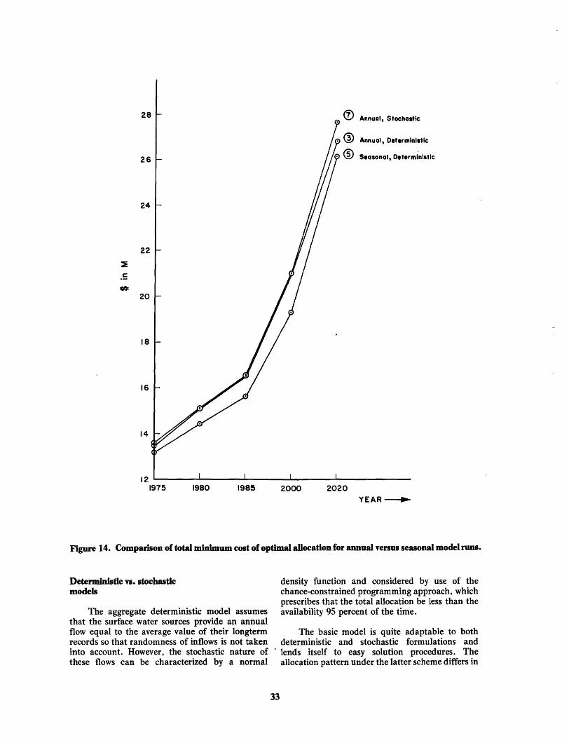
28 ® Annual, Stochastic
.® Annual, Deterministic
26 ® Seasonal, Deterministic
24
22
20
18
16
14
12 ~------~--------------~------~~------------1975 1980 1985 2000 2020
YEA R ------..
Figure 14. Comparison of total minimum cost of optimal allocation for annual versus seasonal model runs.
Detenninistlc vs. stochastic models
The aggregate deterministic model assumes that the surface water sources provide an annual flow equal to the average value of their longterm records so that randomness of inflows is not taken into account. However, the stochastic nature of these flows can be characterized by a normal
density function and considered by use of the chance-constrained programming approach, which prescribes that the total allocation be less than the availability 95 percent of the time.
The basic model is quite adaptable to both deterministic and stochastic formulations and
. lends itself to easy solution procedures. The allocation pattern under the latter scheme differs in
33

Table 11. Wastewater treatment plants utruz.tion.
Areas H2 G F2 F1 E D Model Year TP1 TP2 TP1 TP1 TP2 TP3 TP1 TP1 TP1
Linear 4.5 2.3 5.6 6.0 12.7 0 7.1 33.0 1.5 1975 (81.7)
NLR 4.5 2.3 5.6 9.0 4.0 0 7.1 33.0 1.4 (5.7) (81.8)
LR 4.5 3.9 5.6 8.0 14.2 0 7.8 34.8 1.5 1980 (81.8)
NLR 4.5 3.4 5.6 9.0 5.5 0 7.8 34.3 1.5 (7.7) (.5) (81.8)
1985 LR 4.5 3.9 5.6 9.0 16.2 0 7.8 37.8 1.5
(82.1 ) NLR 4.5 3.9 9.0 6.7 0 7.8 36.4 1.5
(15.1) (82.1 )
LR 4.5 3.9 5.6 9.0 17.9 5.1 7.8 44.3 1.5 2000 (82.6)
NLR 4.5 3.9 9.0 10.8 0 7.8 39.6 1.5 (22.5) (82.6)
LR 4.5, 3.9 5.6 9.0 17.9 5.1 7.8 50.4 (5 2020 (83.3)
NLR 2.3 3.9 7.2 17.9 0 7.8 42.5 1.5 (34.8) (83.3)
The quantities in parentheses indicate additional treatment capacity necessary in the respective subregions.
that the more dependable sources are substituted in place of the variable surface water. In the optimal solutions, surface water is replaced by imported water, which is assumed to be a more reliable source than surface water over time (Table 12).
The system effects on wastewater treatment and reuse are displayed by Figures 15 through 19. As the diagrams shows reuse is required in area H for industrial purposes over the entire planning horizon. Areas E and F show reuse for 1980 at
Level II treatment, but with the Level III regional plant in 1985 reuse is curtailed.
Introduction of stochastic elements into the allocation scheme results in a slight increase of the total allocation cost (lines III and VII, and IV and VIII in Table 10). The increased additional cost comes from additional high cost imported water required by the system. Reuse acitivites increase in the stochastic model only if imported water is insufficient (Figures 15 through 19).
~able 12. Replacement of surface water by import water In optimal solutions for stochastic model.
Year
1975 1980 1985 2000 2020
Surface Water for M&I
Water for M&I
31 /20.2 42.2/20.9 52.5/21.7 72 /48.7 87.7/84.5
Sw forM&I
Iw for M&l
25.8/25.4 40.4/22.7 40.4/35.5 36.2/84.5 40.4/84.5
34
Sw for Ag
Iw for Ag
71.3/ 2.9 63.1/ 2.2 60 / 2.2 40.5/ 1.7 24.8/ 1.2
Iw for Ag
14.6/59.6 o /65.6 o /63.2 o /43.2 o /27
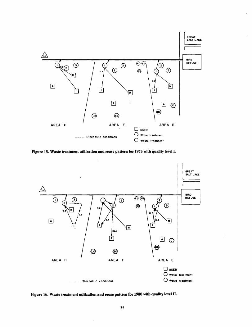
AREA H AREA F
_____ Stochastic conditions
AREA E
o USER
o Water treatment
o Waste treatment
GREAT SALT LAKE
BIRD REFUGE
Figure 15. Waste treatment utiIization and reuse pattem for 1975 with quality level I.
AREA H
, I
I , /9.a ,
I
AREA F
_____ Stachastic conditions
AREA E
o USER
GREAT SALT LAKE
BIRD REFUGE
o Water treatment
o Waste treatment
Figure 16. Waste treatment utilization and reuse pattem for 1980 with quality level ll.
35

AREA H
Stochastic cQnditiQns
o o
AREA F
@
AREA E o USER
o Water treatment
o Waste treatment
Figure 17 • Waste treatment utiUzation and reuse pattem for 1985 with quaDty level ill.
AREA H AREA F AREA E
0 USER
0 Water treatment
_____ Stochastic conditions 0 Waste treatment
Figure 18. Waste treatment utiHzation and reuse pattem In 2000 with quaDty level m.
36
GREAT SALT LAKE
BIRD REFUGE
GREAT SALT .LAKE
BIRD REFUGE

~
0 G) CD
0
~
€9 AREA H AREA
_____ Stochastic conditions
0
F AREA E
o USER
o Water treatment
o Waste treatment
GREAT SALT LAKE
BIRD REFUGE
Figure 19. W ute treatment utlHzation and reue pattem for lOlO with quaDty level m.
Sector allocations under various assumptions
As further illustrations of the types of information that might be derived from various model formulations and model runs, the following paragraphs analyze model results for the major water source, water use and treatment sectors in the model.
Surface water and water treatment plants
Model results based on annual average flows and requirements follows findings (Bishop et aI., 1974) that water treatment plants in the basin presently have the capacity to meet the requirements for water over the projected study period. However, for high demand periods such as summer months (see Table 13), the existing maximum capacity cannot meet the requirements after 2000.
Groundwater
Groundwater is allocated largely to municipal req uirements and very little groundwater is used for other purposes (Table 14). The agricultural sector generally is not allocated any groundwater. Allocation of groundwater in industrial sectors
37
Table 13. Water treatment plants (maximum capacity 209,700 ac-ft/year).
Year Annual Summer Requirementa Requirementb
1975 30,600 82,800 1980 41,800 101,600 1985 54,200 117,400 2000 98,300 179,400 2020 147,600 266,000a
a In ac-ft/year
b Adjusted to ac-ftJyear.
frequently has been replaced by reuse of higher quality effluent, when available. Use of groundwater is increased if dependability of surface water sources is reduced. The utilization of groundwater is increased until the safe yield i~ reached (103,800 ac-ft/year for aggregated model area of study). Seasonal requirements have very little effect upon allocation or use of goundwater.
Reusable sources
The sources available for direct reuse are municipal and industrial effluents. In this study, direct reuSe of effluent in the municipal sector is
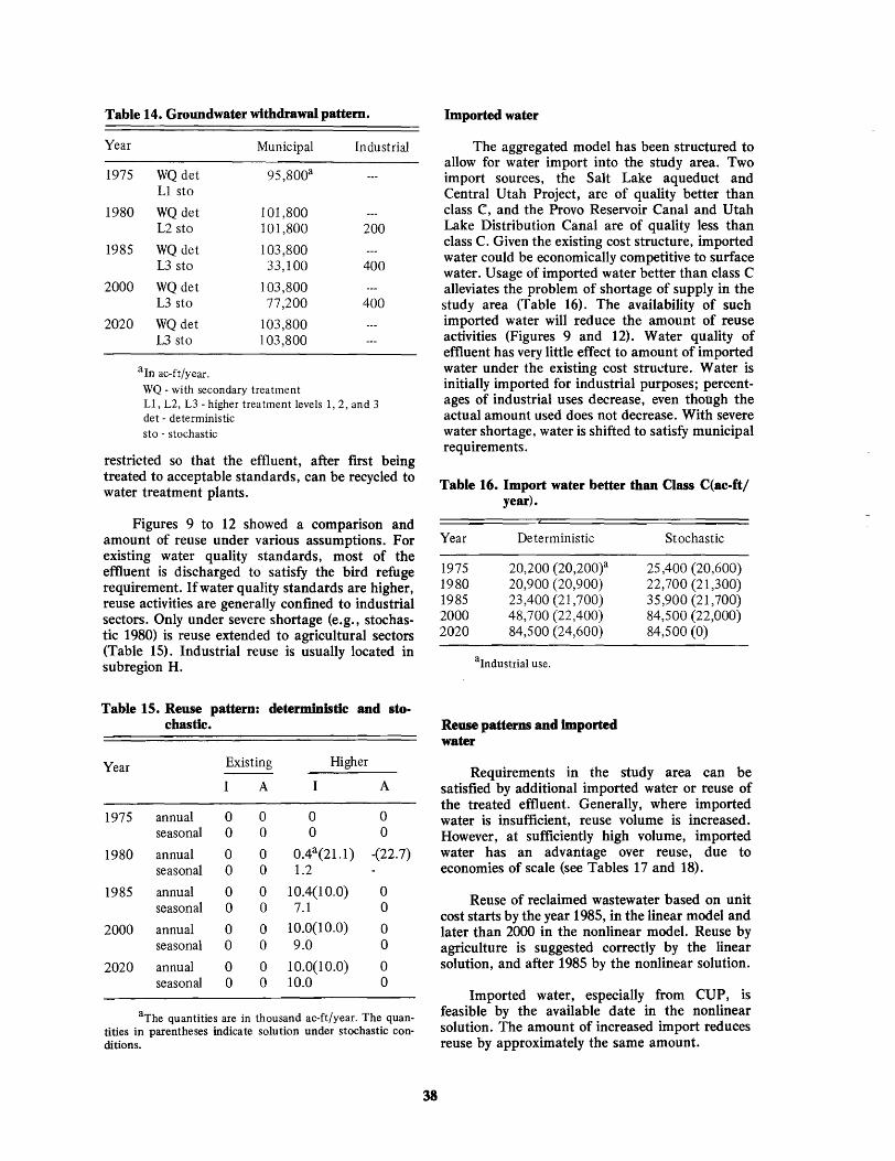
Table 14. Groundwater withdrawal pattern.
Year
1975
1980
1985
2000
2020
Municipal Industrial
WQ det 95,800a
L1 sto
WQ det 101,800 L2 sto 101,800 200
WQ det 103,800 L3 sto 33,100 400
WQ det 103,800 L3 sto 77,200 400
WQ det 103,800 L3 sto 103,800
aIn ac-ft/year. WQ - with secondary treatment Ll, L2, L3 - higher treatment levels 1,2, and 3 det - deterministic sto - stochastic
restricted so that the effluent, after first being treated to acceptable standards, can be recycled to water treatment plants.
Figures 9 to 12 showed a comparison and amount of reuse under various assumptions. For existing water quality standards, most of the effluent is discharged to satisfy the bird refuge requirement. If water quality standards are higher, reuse activities are generally confined to industrial sectors. Only under severe shortage (e.g., stochastic 1980) is reuse extended to agricultural sectors (Table 15). Industrial reuse is usually located in subregion H.
Table 15. Reuse pattern: deterministic and stochastic.
Year Existing Higher
A A
1975 annual 0 0 0 0 seasonal 0 0 0 0
1980 annual 0 0 0.4a(21.1) -(22.7) seasonal 0 0 1.2
1985 annual 0 0 10.4(10.0) 0 seasonal 0 0 7.1 0
2000 annual 0 0 10.0(10.0) 0 seasonal 0 0 9.0 0
2020 annual 0 0 10.0(10.0) 0 seasonal 0 0 10.0 0
aThe quantities are in thousand ac-ft/year. The quan-tities in parentheses indicate solution under stochastic con-ditions.
38
Imported water
The aggregated model has been structured to allow for water import into the study area. Two import sources, the Salt Lake aqueduct and Central Utah Project, are of quality better than class C, and the Provo Reservoir Canal and Utah Lake Distribution Canal are of quality less than class C. Given the existing cost structure, imported water could be economically competitive to surface water. Usage of imported water better than class C alleviates the problem of shortage of supply in the study area (Table 16). The availability of such imported water will reduce the amount of reuse activities (Figures 9 and 12). Water quality of effluent has very little effect to amount of imported water under the existing cost structure. Water is initially imported for industrial purposes; percentages of industrial uses decrease, even though the actual amount used does not decrease. With severe water shortage, water is shifted to satisfy municipal requirements.
Table 16. Import water better than Class C(ac-ft/ year).
Year De terministic
1975 20,200 (20,200)a 1980 20,900 (20,900) 1985 23,400 (21,700) 2000 48,700 (22,400) 2020 84,500 (24,600)
alndustrial use.
Reuse patterns and Imported water
Stochastic
25,400 (20,600) 22,700 (21,300) 35,900 (21,700) 84,500 (22,000) 84,500 (0)
Requirements in the study area can be satisfied by additional imported water or reuse of the treated effluent. Generally, where imported water is insufficient, reuse volume is increased. However, at sufficiently high volume, imported water has an advantage over reuse, due to economies of scale (see Tables 17 and 18).
Reuse of reclaimed wastewater based on unit cost starts by the year 1985, in the linear model and later than 2000 in the nonlinear model. Reuse by agriculture is suggested correctly by the linear solution, and after 1985 by the nonlinear solution.
Imported water, especially from CUP, is feasible by the available date in the nonlinear solution. The amount of increased import reduces reuse by approximately the same amount.

Table 17. Reuse comparisons: Linear vs. nonlinear model, municipal and industrial emuent for M, I, and agricultural uses.
M & I Uses Agricultural Uses Year
Linear Nonlinear Linear Nonlinear
1975 1980 1985 2000 2020
oa o
2,120 15,320 22,900
a All figures in acre-feet.
o o o o
14,200
7,000 5,900 5,180 4,700
14,800
o o
1,400 4,700 9,300
Table 18. Import water comparisons between lInear and nonlinear models (municipal use).
Year Linear Nonlinear
1975 14.5a 14.5 1980 14.5 14.5 1985 14.5 34.0 2000 14.5 66.7 2020 70.6 84.5
a Acre-feet in thousands.
Economies of scale play a significant role in allocation. Depending on the degree of difference from the average unit cost, allocations can change significantly.
Wastewater treatment plants
Existing wastewater treatment facilities in subregion H need to be expanded by 1980 and probably replaced by 2020. The facilities in subregion F also need to be expanded by the year 2000, particularly with higher standards for effluent discharge (Tables 19a, b). However, according to the seasonal model, the expansion of facilities in both regions could be postponed a few more years. Only in region E is present wastewater treatment capacity sufficient until 2020.
To meet the required standard of effluent discharge in 1980, wastewater treatment plants capable of upgrading effluent to Level II are needed in all regions. In 1985, wastewater treatment plants to upgrade effluent to Level III are needed for effluents from region H and regions F and E. The treatment plant schedule also applies under seasona1 variations, but the required capacities are different.
Table 198. Required wastewater treatment plant. capacity (100 ac-ft/year) (a) existing quality: annual vs. seasonal.
Region 1975 1980 1985 2000 2020
H annual 6.8 9.8a 11.2a 15.7a 22.9b seasonal 4.4 6.2 7.2 10.0 14.6
F annual 31.4 36.1 40.0 54.8a 77.0; seasonal 20.2 23.0 25.6 35.0 48.0
E annual 33.0 34.3 36.4 39.6 42.5 seasonal 24.0 25.0 26.4 28.6 31.2
aCapacity expansion needed.
bNew treatment plants will have to be built.
Table 19b. Required wastewater treatment plants capacity (100 ac-ft/year) (b) hlaher quality: annual VI.
seasonal.
Year Region
F H exis L2 L3 ex is L2 L3 exis L2
1975 annual 6.8 seasonal 4.4
1980 annual 9.8 seasonal 6.2
1985 annual 8.4 11.2 0.8 seasonal 7.2 7.2
2000 annual 8.4 15.7 5.7 seasonal 8.4 10.0
2020 annual 22.9 12.9 seasonal 8.4 10.0 6.2
31.4 20.2
36.1 36.1 23.0 23.0
39
33.0 24.0
34.3 34.3 25.0 25.0
E Regional L3 Ll L2 L3
76.4 62.0
94.4 73.6
119.5 80.2

Computer TliDe/Cost ComparISOns
The model was solved using the Lambda fornlUlation of the separable progrartuhirig technique. A standard mathematical programming system (TEMPO), available with the Burrough's 6700, was used. Some of the important statistics of the program are discussed as follows.
In the separable formulation of the nonlinear cost function associated with the variable xii' the polygonal approximation of the functionS are arrived at as follows. Assuming all xii to l\~ betWeeh o and 250,000 acre-feet, five grid pofnts Xij, k = 1, 2 ... S, were chosen in this range.
o 1,000 10,000 50,000250,000 x ij
X~j = 0; xij = 1 ,000; X~j = 10,000; xiJ = 50,000;
X~j = 250,000
The dec~ion variables are no longer xi" s but they are the Aij. Once the As are determine op\imally, the xij, the optimal Xij can be calculated with
40
X~ = ~ At x ~ for all i and j
In order to avoid hand computation of the optimal Xjj' the above equation was defined as a free row in ttfe problem. The restricted basis entry was implemented so that the A variables entering the basis will always be adjacent.
In the seven-region model, there are 1010 variables in xii and five grid points which result in 5050 A variar>les. There are 100 constraints of which 40 were iIi equalities and 60 were fixed rows. in addition, there were 1010 fixed rows corresponding to the constraints
L A~ = 1 k IJ
for all i and j
Corresponding to 1010 variables of Xij' 1010 constraints were defined as free rows. In aH.dition, the objective function is a free row. Thus, there were 5050 variables and 2120 rows, or which 1110 were constraints. The cost of obtaining an optimal solution was as high as $450. Using an old basis, solutions to moqified problems were obtained at an average cost of $90. The CPU time averaged 450 seconds for these runs and the memory requirement was about 17,500 kw/sec.
The three-region nonlinear model had 2079 variables and 644 rows, of which 356 were constraints. Solutions took about 100 sec. of CPU time and the memory requirement was about 2000 kw/sec. The cost of solutions obtained by starting from an old basis averaged about $20.
The linear solution cost is roughly about one tenth of the nonlinear solution, given similar starting conditions. Linear solutions were obtained using MPS/360 (IBM package) while the nonlinear solutions were obtained using TEMPO (Burrough's package).

REFERENCES
Aron, G., and V. H. Scott. 1971. Dynamic programming for conjunctive water use. ASCE, Journal of the Hydraulics Division 97(HY5):705.
Bayer, M. B. 1974. Nonlinear programming in river basin modeling. Water Resources Bulletin 10(2) :311-317 .
Berthouex, P. M. 1972. Evaluating economics of scale. Journal Water Pollution Control Federation 44:2111-2119.
Bishop, A. B., and D. W. Hendricks. 1971. Water reuse systems analysis. Water Resources Bulletin 7(3):542-553. June.
Bishop, A. B., W. J. Grenney, R. Narayanan, and S. L. Klemetson. 1974. Evaluating water reuse alternatives in water resource planning. Utah Water Research Laboratory, PRWG123-1, Utah State University, Logan, Utah.
Boehm, L. 1973. Should industry purchase or seek its own supply of water. Journal American- Water Works Association 65:332.
Burroughs. 1973. Mathematical programming system user manual. TEMPO 6700. Burroughs Corp. Detroit, Michigan.
r
Butcher, W. S., Y. Y. Haimes, and W. A. Hall. 1969. Dynamic programming for the optimal sequencing of water supply projects. Water Resources Research 5(6):1196-1204.
Charnes, A., and W. W. Cooper. 1963. Deterministic Equivalents for optimizing and satisfying under chance constraints. Operations Research, Vol. 11, pp. 18-39.
Clyde, C. G., A. B. King, and J. C. Andersen. 1971. Application of operations research techniques for allocation of water resources in Utah. Utah Water Research Laboratory, PRWG 73-2. Utah State University, Logan, Utah.
Dawes, J. H. 1970. Tools for water resources study. Journal Irrigation and Drainage Division. American Society of Civil Engineers IR4:403.
DeVries, R. N., and C. G. Clyde. 1971. Optimization in municipal water supply system design. Water Resources Bulletin 7(5): 1048.
Eckenfelder, W. W., and C. E. Adams, Jr. 1972. Design and economics of joint wastewater treatment. Journal Sanitary Engineering Division, American Society of Civil Engineers 98:153.
Engineering News Record. 1974. Construction scoreboard. McGraw-Hill Publishers, weekly publication.
Engineering-Science. 1970. Deepwater interceptor feasibility study report. Prepared for Delaware River Basin Commission, Trenton, New Jersey.
Evenson, D. E .. G T. Orlob. and J. R. Monser. 1969. Preliminary section of wastewater treatment systems. Journal of Water Pollution Control Federation 41:1845-1858.
41
Environmental Protection Agency and Sanitation Districts of Los Angeles County. 1971. Advanced waste treatment research facility -Pomona, California.
Federal Water Pollution Control Administration. 1967. Sewer and sewage treatment plant construction cost index. U.S. Government Printing Office, Washington, D.C.
Haimes,Y. Y., and W. S. Naiuis. 1974. Coordination of regional water resource supply and demand planning models. Water Resources Research. Forthcoming.
Haimes. Y. Y .. M. A. Kaplan. and M. A. Husar. 1972. A multilevel approach to determining optimal taxation for the abatement of water pollution. Water Resources Research 8(2): 19-26.
Harl, E. N., R. A. Baldwin, and D. W. Hubly. 1971. An analysis of the economic implications of the permit system of water allocation. Iowa State Water Resources Research Institute, Ames, Iowa. ,
Hinomoto, H.1972. Dynamic programming of capacity expansion of municipal water treatment system. Water Resources Research 8(5): 1178-1187 .
Hughes, T. C., and Calvin G. Clyde. 1973. Municipal water planning-mixed interger approach. Journal of the Hydraulics Division HY11:2079-2095. November.
Keith, John E., Jay C. Andersen, and Calvin G. Clyde. 1973. The economic efficiency of inter-basin agricultural water transfers in Utah: A mathematical programming approach. Utah Water Research Laboratory PRWG100-3. Utah State University, Logan, Utah.
Klemetson, S. L. 1974. Development of a dynamic programming model for the regionalization and staging of wastewater treatment plants. PhD. dissertation, Utah State University, Logan.
Koenig. L. 1967. The cost of water treatment by coagulation, sedimentation, and rapid sand filtration. Journal of the American Water Works Association 59:290.
Liebman, J. C., and H. M. David. 1968. Balas algorithm for zoned uniform treatment. Journal of Sanitary Engineering Division. American Society of Civil Engineers. 94(SA4):585-593.
Liebman, J. C., and W. R. Lynn. 1966. The optimal allocation of stream dissolved oxygen. Water Resources Research 2(3): 581-591.
Linaweaver, F. P., Jr., and C. S. Clark. 1964. Cost of water transmission cost. Journal American Water Works Association 56:1549.
Lofting, E. M., and P. H. McGauhey. 1968. Economic evaluation of water, Part IV: An input-output and linear programming analysis of California water requirements. Water Resources Center. University of California, Berkeley, California.
Loucks, D. P., C. S. Revelle, and W. R. Lynn. 1967. Linear programming m9dels for water pollution contr91. Managemept Science 14(4):B166-188.
Lynn, W. R. 1964. Stage development of wastewater treatment works. Journal Water Pollution Control Federation 36(6): 722-751.
Lynn, W. R. 1966. Application of systems analysis to water and wastewater treatment. Journal of the American Water Works Association 58(6):651-656.
Lynn, W. R., J. A. ~gan, and A. Charpes. 1962. Systems analysis for planning wastewater treatment plants. Journal Water Pollution Control Federation 34(6):565-581.
Milligan, J. H. 1969. Optimizing conjunctive use of groundwater and surface water. Utah Water neseareb Laboratory, PRWG42-4. Utah State U~iversity. Logan. Utah. .
Morin, T. L. 1973. Optimal sequencing of capacity eXPaDs.on projects. American Society of Civil Engineers. Journal Hydraulics Division 99(HY9):1605.
Mulvihill, E. M., and J. A. Dracup. 1974. Optimal timing and sizing of a conjunctive urban water supply and wastewater system with nonlinear programming. Water Resources Research 10(2):170-175.
Regev, Uri, and Aba Schwartz. 1973. Optimal path of iI:lterregional investment and allocation of water. Water ~-sources Research 9(2):251-262. .
42
Smith, R. 1968. Cost of conventional and advanced treatment of wl!.!!tewater. Journal Water Pollution Control Federation 4O:i546.
Smith, Ro, and R. G. Eilers. 1970. Cost to the consumer of collecting and treating wastewater in the United States. U.S. Department of the Interior, Federal Water Quality' Admin~tration, Advanced Waste Treatment Branch, Division of Research, Cincinnati, Ohio.
U.S. Departwent of Commerce. 1974. Construction review. Cost and Prices 20(2):44.
U.S. Labor Statistics Bureau. 1974. Employment and earnings. Table C-2, Transportation and Public Utilities, SIC Code 494-7, Water. Steam, and Sanitary Systems (monthly publication).
Walker, W. R., and G. V. Skogerboe. 1973. The impact of water quality-objectives of urban water supply planning. Water Resources Bulletin 9(5):861.
Windsor, J. S., and V. T. Chow, 1972. Multireservoir optimization model. American Society of Civil Engineers 98(HYI0): 1827-1845.
Young, G. K., and M. S. Pisano. 1970. Nonlinear programming applied to regional water resource planning. Water Resources Research 6(1):32-42.
APPENDICES
43

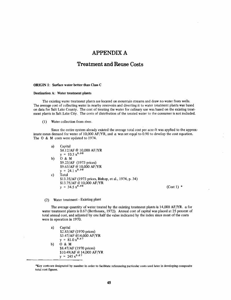
APPENDIX A
Treatment and Reuse Costs
ORIGIN 1: Surface water better than Class C
Destination A: Water treatment plants
The existing water treatment plants are located on mountain streams and draw no water from wells. The average cost of collecting water in nearby reservoirs and diverting it to water treatment plants was based on data for Salt Lake County. The cost of treating the water for culinary use was based on the existing treatment plants in Salt Lake City. The costs of distribution of the treated water to the consumer is not included.
(l) Water collection from river.
Since the entire system already existed the average total cost per acre-ft was applied to the approximate mean demand for water of 10,000 AF /YR, and a was set equ,al to 0.90 to develop the cost equation. The 0 & M costs were updated to 1974.
a) Capital $~.12/ AF @ 10,000 AF /YR y = 10.3xo.9o
b) 0 & M $9.23/AF (1973 prices) $9.63/AF @ 10,000 AF/YR y = 24.1 XO.90
c) Total $13.35/AF (1973 prices, Bishop, et al., 1974, p. 34) $13.75/AF @ 10,000 AF/YR y = 34.5 XO.90
(2) Water treatment - Existing plant
(Cost 1) *
The average quantity of water treated by the existing treatment plants is 14,000 AF /YR. a for water treatment plants is 0.67 (Berthouex, 1972). Annual cost of capital was placed at 25 percent of total annual cost, and adjusted by one half the value indicated by the index since most of the costs were in operation in 1970.
a) Capital $2.83/AF (1970 prices) $3.47/AF @14,000 AF/YR y = 81.0 X O•6 7
b) 0 & M $8.4 7 / AF (1970 prices) $10.49/AF @ 14,000 AF/YR y = 245 xO•6 7
*Key costs are designated by number in order to facilitate referencing particular costs used later in developing composite total cost figures.
4S
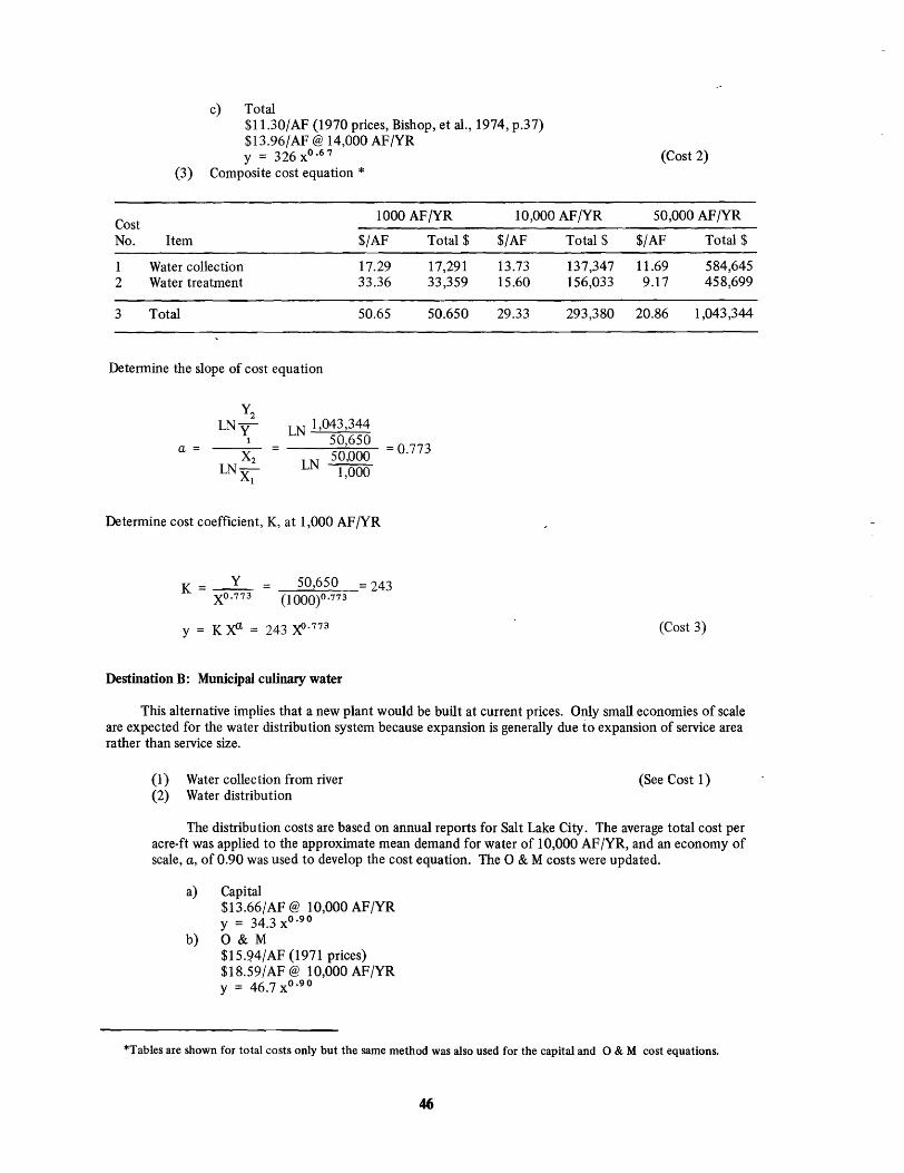
Cost No.
1 2
3
c) Total $11.30/AF (l970 prices, Bishop, et al., 1974, p.37) $13.96/AF @ 14,000 AF/YR y = 326 XO.67
(3) Composite cost equation *
1000 AF/YR 10,000 AF /YR
Item $/AF Total $ $/AF Total $
Water collection 17.29 17,291 13.73 137,347 Water treatment 33.36 33,359 15.60 156,033
Total 50.65 50.650 29.33 293,380
(Cost 2)
50,000 AF/YR
$/AF Total $
11.69 584,645 9.17 458,699
20.86 1,043,344
Detennine the slope of cost equation
a =
LN 1,043,344
50,650 = 0.773 LN 50,000
1,000
Detennine cost coefficient, K, at 1,000 AF /YR
K = _Y_ = 50,650 = 243 XO. 773 (I 000)°·773
Y = K xa = 243 )f.773 (Cost 3)
Destination B: Municipal culinary water
This alternative implies that a new plant would be built at current prices. Only small economies of scale are expected for the water distribution system because expansion is generally due to expansion of service area rather than service size.
(l) Water collection from river (2) Water distribution
(See Cost 1)
The distribution costs are based on annual reports for Salt Lake City. The average total cost per acre-ft was applied to the approximate mean demand for water of 10,000 AF/YR, and an economy of scale, a, of 0.90 was used to develop the cost equation. The 0 & M costs were updated.
a) Capital $13.66/AF @ 10,000 AF/YR y = 34.3 XO •90
b) 0 & M $15.94/AF (l971 prices) $18.59/AF @ 10,000 AF/YR y = 46.7 X O •90
*Tables are shown for total costs only but the same method was also used for the capital and 0 & M cost equations.
46
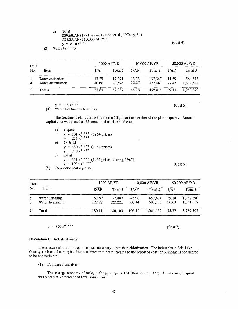
Cost No.
1 4
5
Cost No.
5 6
7
c) Total $29.60/AF (1971 prices, Bishop, et al., 1974, p. 34) $32.25/AF @ 10,000 AF/YR y = 81.0xO.90 (Cost 4)
(3) Water handling
1000 AF/YR 10,000 AF /YR 50,000 AF/YR
Item $/AF Total $ $/AF Total $ $/AF Total $
Water collection 17.29 17,291 13.73 137,347 11.69 584,645 Water distribution 40.60 40,596 32.25 322,467 27.45 1,372,644
Totals 57.89 57,887 45.98 459,814 39.14 1,957,890
y = 115xo.9o (Cost 5) (4) Water treatment - New plant
The treatment plant cost is based on a 50 percent utilization of the plant capacity. Annual capital cost was placed at 25 percent of total annual cost.
a) Capital y = 131 XO.692 (1964 prices) y = 256 XO.692
b) 0 & M y = 430 XO.692 (1964 prices) y = 770 XO .692
c) Total y = 561 XO. 692 (1964 prices, Koenig, 1967) y = 1026xo.692
(5) Composite cost equation
1000 AF/YR 10,000 AF/YR
Item $/AF Total $ $/AF Total $
Water handling 57.89 57,887 45.98 459,814 Water treatment 122.22 122,221 60.14 601,378
Total 180.11 180,103 106.12 1,061,192
y = 829 XO. 779
(Cost 6)
50,000 AF /YR
$/AF Total $
39.14 "I ,957,890 36.63 1,831,617
75.77 3,789,507
(Cost 7)
Destination C: Industrial water
It was assumed that no treatment was necessary other than chlorination. The industries in Salt Lake County are located at varying distances from mountain streams so the reported cost for pump age is considered to be approximate.
(1) Pumpage from river
The average economy of scale, a, for pump age is 0.51 (Berthouex, 1972). Anual cost of capital was placed at 25 percent of total annual cost.
47

a) Capital $1.96/AF (1971-72 prices) $2.32/AF @ 19,363 AF/YR y = 292xo.51
b) 0 & M $5.86/AF (l971-72 prices) $6.60/AF @ 19,363 AF/YR y = 832 X O •5 1
c) Total $7.82/AF (l971-72 prices, Boehm, 1973) $8.92/AF @ 19,363 AF/YR y = 1124xo.51
(2) Chlorination a) Annual capital cost
y = 9.18 XO.658 (l967 prices, Smith, 1968, Figure 16)
y = 16.3 X O•6 5 8
b) Annual 0 & M costs y = 6.05 XO.
897 (l967 prices, Smith, 1968, Figure 16) y = 9.35 XO. 897
c) Chlorination equation '
1000 AF/YR 10,000 AF /YR Cost No. Item
Annual Capital O&M
9 Total
Cost No.
8 9
10
y = 16.7 XO.855
(3) Water handling
Item
Water pump age Chlorination
Total
y = 725 XO. 595
(4) Composite cost equation y = 725 xo. 5 9 5
Destination D: Agricultural water
(l) Diversion structures
$/AF Total $ $/AF Total $
1.54 1,535 0.70 6,985 4.59 4,590 3.62 36,208
6.13 6,125 4.32 43,193
1000 AF/YR 10,000 AF /YR
$/AF Total $ $/AF Total $
38.09 38,086 12.32 123,244 6.13 6,125 4.32 43,193
44.22 44,211 16.64 166,437
(Cost 8)
50,000 AF /YR
$/AF Total $
0.40 20,142 3.07 153,381
3.47 173,529
(Cost 9)
50,000 AF /YR
$/AF Total $
5.60 280,054 3.47 173,529
9.07 453,5'83
(Cost 10) (See Cost 10) (Cost 11)
Large economies of scale are possible with diversion structures, but since the actual cost is very dependent upon the terrain, an average value of a = 0.90 has been used. Annual cost of capital was placed at 75 percent of total annual cost.
48

Cost No.
12 13
14
a) Capital $0.53/AF (1973 prices) $0.57/ AF @ 1960 AF /YR y = 1.18 XO.90
b) 0 & M $0.18/AF (1973 prices) $0.19/AF @ 1,460 AF/YR Y = 0.39 XO
•90
c) Total $0.71/AF (1973 prices, Bishop et aI., 1974, p. 36) $0.76/AF @ 1,460 AF/YR y = 1.57xo.90
(2) Canal costs
(Cost 12)
Assuming that.a canal is used by several farms, or industries, the cost equation represents the total cost of building and operating one mile of canal. The annual cost of capital was placed at 75 percent of the total annual cost. An economy of scale, a, of 0.26 was used (Linaweaver and Clark, 1964, Table 7). Since most of the canal system is already in existence, the cost of capital was increased only one half of that indicated by the cost index.
a) Capital $2.39/ AF /mi (1962 prices, Bishop et al., 1974, p. 36) $2.4 7/ AF /mi @ 22,393 AF /YR y = 4,091 XO •2 6
b) 0 & M $0.80/ AF /mi (1962 prices) $1.50/ AF /mi @ 22,393 AF /YR y = 2,484 XO.26
c) Total $3.19/ AF /mi (1962 prices) $3.97/AF/mi @ 22,393 AF/YR Y = 6,575 XO. 26
(3) Water handling
1000 AF/YR 10,000 AF/YR
Item $/AF Total $ $/AF Total $
Diversion 0.79 787 0.63 6,250 Canal 39.62 39,618 7.21 72,093
Total 40.41 40,405 7.84 78,343
y = 4,747 XO. 31
(4) Composite cost equation Y = 4,747 XO. 31
(Cost 13)
50,000 AF /YR
$/AF Total $
0.53 26,605 2.19 109,554
2.72 136,159
(Cost 14) (See Cost 14) (Cost 15)
ORIGIN 2: Water treatment plant
Destination B: Municipal culinary water
Since the water treatment plant is providing culinary water, only the cost of distributing the water is incurred
49
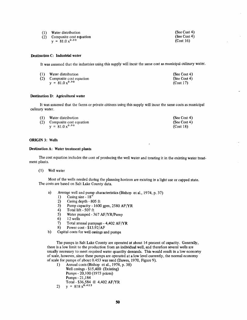
(1) (2)
Water distribution Composite cost equation y = 81.0 XO.90
Destination C: Industrial water
(See Cost 4) (See Cost 4) (Cost 16)
It was assumed that the industries using this supply will incur the same cost as municipal culinary water.
(1) Water distribution (2) Compbsite cost equation
y = 81.0xO. 90
Destmation b: Agricultural water
(See Cost 4) (See Cost 4) (Cost 11)
It Was assumed that the farms or private citizens using this supply will incur the same costs as municipal culinary water.
(1) Water distribution (2) Composite cost equation
y = 81.0 XO.90
ORIGIN 3: Wells
Destination A: Water treatment plants
(See Cost 4) (See Cost 4) (Cost 18)
The cost equation includes the cbst of producing the well water and treating it in the eXisting water treatment plants.
(1) Well water
Most of the wells needed during the planning horizon are existing in a light use or capped state. The costs are based on Salt Lake County data.
a) Average well and pump characteristics (Bishop etal., 1974, p. 37) 1) Casing size - 18" 2) Casing depth - 805 ft 3) Pump capacity - 1600 gpm, 2580 AF /YR 4) Total lift - 507 ft 5) Water pumped - 367 AF /YR/Pump 6) 12 wells 7) Total annual pumpage - 4,402 AF/YR 8) Power cost - $13.92/AF
b) Capital costs for well casings and pumps
The pumps in Salt Lake County are operated at about 14 percent of capacity. 'Generally, there is a low limit to the production from an individual well, and therefore several wells are usually necessary to meet required water quantity demands. This would result in a low economy of scale, however, since these pumps are operated at a clow level currently, the normal economy of scale for pumps of about 0.453 was used (Dawes, 1970, Figure 9).
1) Annual costs (Bishop et aI., 1974, p. 38) Well casings - $15,400 (Existing) Pumps - 20,100 (1973 prices) Pumps - 21,184 Total - $36,584 @ 4,402 AF /YR
2) y = 818 XO.453
50
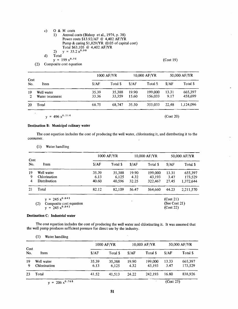
Cost No.
19 2
20
c) 0 & M costs 1) Annual costs (Bishop et al., 1974, p. 38)
Power costs $13.92/AF @ 4,402 AF/YR Pump & casing $1,829/YR (0.05 of capital cost) Total $63,105 @ 4,402 AF/YR
2) y = 33.2 X O•90
d) Total y = 199 XO. 75
(2) Composite cost equation
1000 AF/YR 10,000 AF/YR
Item $/AF Total $ $/AF Total $
Well water 35.39 35,388 19.90 199,000 Water treatment 33.36 33,359 15.60 156,033
Total 68.75 68,747 35.50 355,033
y = 496 XO . 714
Destination B: Municipal culinary water
(Cost 19)
50,000 AF/YR
$/AF Total $
13.31 665,397 9.17 458,699
22,48 1,124,096
(Cost 20)
The cost equation includes the cost of producing the well water, chlOrinating it, and distributing it to the consumer.
(l) Water handling
Cost No. Item
19 Well water 9 Chlorination 4 Distribution
21 Total
(2) y = 245 XO. S42
Composite cost equation y = 245 XO. S42
Destination C: Industrial water
1000 AF/YR
$/AF Total $
35.39 35,388 6.13 6,125
40.60 40,596
82.12 82,109
10,000 AF/YR 50,000 AF /YR
$/AF Total $ $/AF Total $
19.90 199,000 13.31 655,397 4.32 43,193 3.47 173,529
32.25 322,467 27.45 1,372,644
56.47 564,660 44.23 2,211,570
(Cost 21) (See Cost 21) (Cost 22)
The cost equation includes the cost of producing the well water and chlorinating it. It was assumed that the well pump produces sufficient pressure for direct use by the industry.
(l) Water handling
1000 AF/YR 10,000 AF /YR 50,000 AF /YR Cost No. Item $/AF Total $ $/AF Total $ $/AF Total $
19 Well water 35.39 35,388 19.90 199,000 13.33 665,397 9 Chlorination 6.13 6,125 4.32 43,193 3.47 173,529
23 Total 41.52 41,513 24.22 242,193 16.80 838,926
y = 206 XO. 768 (Cost 23)
S1

(2) Composite cost equation y = 206 xO. 768
Destination D: Agricultural water
It was assumed that the wells are located on the farms, and are used directly.
(1) Well water (2) Composite cost equation
y = 199 XO. 75
ORIGIN 4: Municipal effluent
Destination E: Existing secondary treatment plants
(See Cost 23) (Cost 24)
(See Cost 19) (See Cost 19) (Cost 25)
The cost equation includes the costs of collecting the wastewater from the sources and treating it in the existing secondary treatment plants.
(1) Sewage collection
The cost of sewage collection is based on the Salt Lake City data using the national averages of cost for 1968. Since most of the system already exists, the values were not adjusted to higher current costs.
a) National sewer collection data (Smith & Eilers, 1970) 1) Capital
House connection Municipal sewers Interceptors and outfa11s
2) 0 & M
$ 1.38 8.64 2.46
$ 12,48/Capita/YR
Municipal sewer maintenance $ 0.86 Customer Service and Accounting 0.36 General and Administration 0.69
$ 1.91/Capita/YR b) Economy of scale (Smith & Eilers, 1970, Table III)
a = 0.91 c) Data for Salt Lake City (Bishop et aI., 1974, p. 39)
Wastewater flow = 33.4 mgd = 37,300 AF /YR Population (1970) = 174,870
d) Capital @ 37,300 AF /YR $12.48/Capita/YR x 174,870 = $2,182,378 y = 151 XO•91
e) 0 & M @ 37,300 AF/YR $1.91/Capita/YR x 174,870 = $334,002 y = 23 XO. 91
f) Total @ 37,300 AF/YR $14.39/Capita/YR x 174,870 = $2,516,379 y = 174xo.91
(2) Existing secondary treatment plant (Cost 26)
These plants exist, therefore, the reported ca:pital costs for 1967 were used and the 0 & M costs were updated to 1974.
a) Capital - Trickling fIlter plants y = 137 XO.
784 (1967 prices, Smith, 1968, Figure 7)
S2
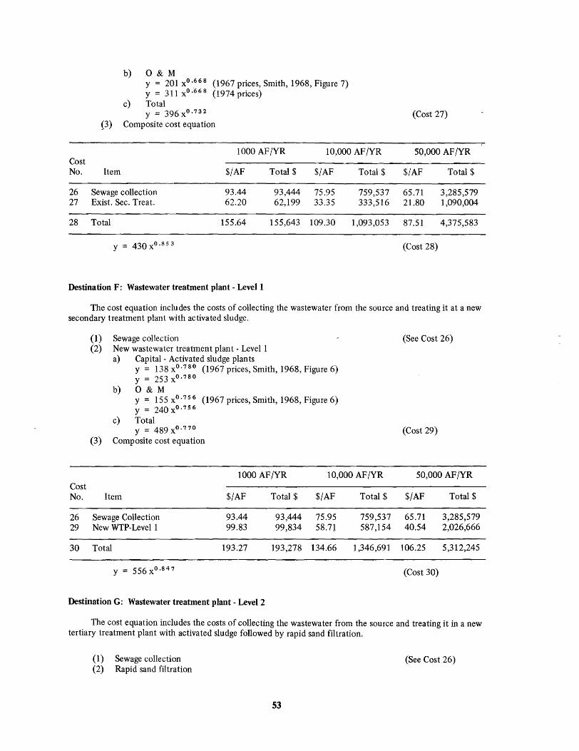
b) 0 & M Y = 201 XO.668 (1967 prices, Smith, 1968, Figure 7) y = 311 XO.668 (1974 prices)
c) Total y = 396 XO. 732
(3) Composite cost equation
1000 AF/YR 10,000 AF/YR Cost No. Item $/AF Total $ $/AF Total $
26 Sewage collection 93.44 93,444 75.95 759,537 27 Exist. Sec. Treat. 62.20 62,199 33.35 333,516
28 Total 155.64 155,643 109.30 1,093,053
y = 430 XO.8 53
Destination F: Wastewater treatment plant - Levell
(Cost 27)
SQ,OOO AF /YR
$/AF Total $
65.71 3,285,579 21.80 1,090,004
87.51 4,375,583
(Cost 28)
The cost equation includes the costs of collecting the wastewater from the source and treating it at a new secondary treatment plant with activated sludge.
{l) Sewage collection (2) New wastewater treatment plant - Levell
a) Capital - Activated sludge plants y = 138 XO. 780 (1967 prices, Smith, 1968, Figure 6) y = 253 XO. 780
b) 0 & M Y = 155 XO. 756 (1967 prices, Smith, 1968, Figure 6) y=240xO. 756
c) Total y = 489 XO. 770
(3) Composite cost equation
1000 AF/YR 10,000 AF /YR Cost No. Item $/AF Total $ $/AF Total $
26 Sewage Collection 93.44 93,444 75.95 759,537 29 New WTP-Level1 99.83 99,834 58.7J 587,154
30 Total 193.27 193,278 134.66 1,346,691
y = 556 XO. 847
Destination G: Wastewater treatment plant - Level 2
(See Cost 26)
(Cost 29)
50,000 AF /YR
$/AF Total $
65.71 3,285,579 40.54 2,026,666
106.25 5,312,245
(Cost 30)
The cost equation includes the costs of collecting the wastewater from the source and treating it in a new tertiary treatment plant with activated sludge followed by rapid sand filtration.
(1) Sewage collection (2) Rapid sand filtration
S3
(See Cost 26)

a) Capital y = 51.8 XO.
662 (1967 prices, Smith, 1968, Figure 9) y = 95.0 XO. 662
b) 0 & M y = 252 XO. 6
3 8 (1967 prices, Smith, 1968, Figure 9) y = 390 XO .6 3 8
c) Total y = 481 XO.644
(3) New wastewater treatment plant - Level 2
1000 AF/YR 10,000 AF /YR Cost No. Item $/AF Total $ $/AF Total $
29 New WTP-Levell 99.83 99,834 58.71 587,154 31 Rapid sand filter 41.13 4.1,129 18.12 181,195
32 Total 140.96 140,963 76.83 768,349
y = 855 XO. 739
(4) Composite cost equation
1000 AF/YR 10,000 AF/YR Cost No. Item $/AF Total $ $/AF Total $
26 Sewage collection 93.44 93,444 75.95 759,537 32 New WTP-LeveI2 140.96 140,963 76.83 768,349
33 Total 234.40 234,407 152.78 1,527,886
y = 807 XO. 821
Destination H: Wastewater treatment plant - Level 3
(Cost 31)
50,000 AF /YR
$/AF Total $
40.54 2,026,666 10.22 510,836
50.76 2,537,502
(Cost 32)
50,000 AF/YR
$/AF Total $
65.71 3,28?,579 50.76 2,537,502
116.47 5,823,081
(Cost 33)
The cost equation includes the costs of collecting the wastewater from the source and treating it in a new tertiary treatment plant with activated sludge followed by rapid sand ftltration and carbon adsorption.
(1 ) Sewage collection (2) Carbon adsorption
a) Capital y = 281 XO.
626 (1967 prices, Smith, 1968, Figure 11) y = 515 XO.626
b) 0 & M y = 226 XO .724 (1967 prices, Smith, 1968, Figure 11) y = 349 XO. 724
c) Total y = 794 XO.686
(3) New wastewater treatment plant - Level 3
54
(See Cost 26)
(Cost 34)

Cost No. Item
29 New WI'P-Level 1 31 Rapid san~ fIlter 34 Carbon adsorption
35 Total
y = 1,603 XO. 72O
(4) Composite cost equation
Cost No. Item
26 Sewage collection 35 New WTP-LeveI3
36 Total
y = 1,387 XO. 79
l000AF/yR
$/AF Total $
99.83 99,83,4 41.1~ 41,129 90.74 90,745
231.70 231,708
1000 AF/YR
$/AF Total $
93.44 93,444 231.70 231,708
325.14 325,152
Destination I: Wastewater treatment plant - Reuse
10,000 AF/yR 50,000 AF /YR
$/AF Total $ $/AF Total $
58.71 587,154 40.54 2,026~666 18.12 181,19S 10.22 510,836 44.04 440,373 26.57 1,328,354
120.87 1,208~722 77.33 3,865,856
(Cost 35)
10,000 AF/YR 50,000 AF /YR
$/AF Total $ $/AF Total $
75.95 759,537 65.71 3,285,579 120.87 1,208,722 77.33 3,865,856
196.82 1,968,259 143.04 7,151;435
;
(Cost 36)
The cost equation includes the costs of collecting the wastewater from the source and treating it in a new tertiary treatment plant to a quality suitable for direct use as culinary water. The plant ~onsists of an activated sludge process followed by rapid sand fIltration, carbon adsorption, and ion exchange.
(1 ) Sewage collection (2) Ion exchange;
(See Cost 26)
One third of the flow of the plant is processed through the ion exchange unit and then blended with the remaining flow.
a) Capital y = 86 XO.841 (1970 prices, EPA, 1971) Y = 128 XO.841 ,
Y = 42.7 XO.841 (33% blend) b) 0 & M
y = 531 XO .841 (1970 prices, EPA, 1971) y = 658xo.841
Y = 219 xO.841 (33% blend) c) Total
y = 617 XO.841 (1970 prices, EPA, 1971) y = 786 XO.841
Y = 262 XO.841
(3) New wastewater treatment plant - Reuse
55
(Cost 37)
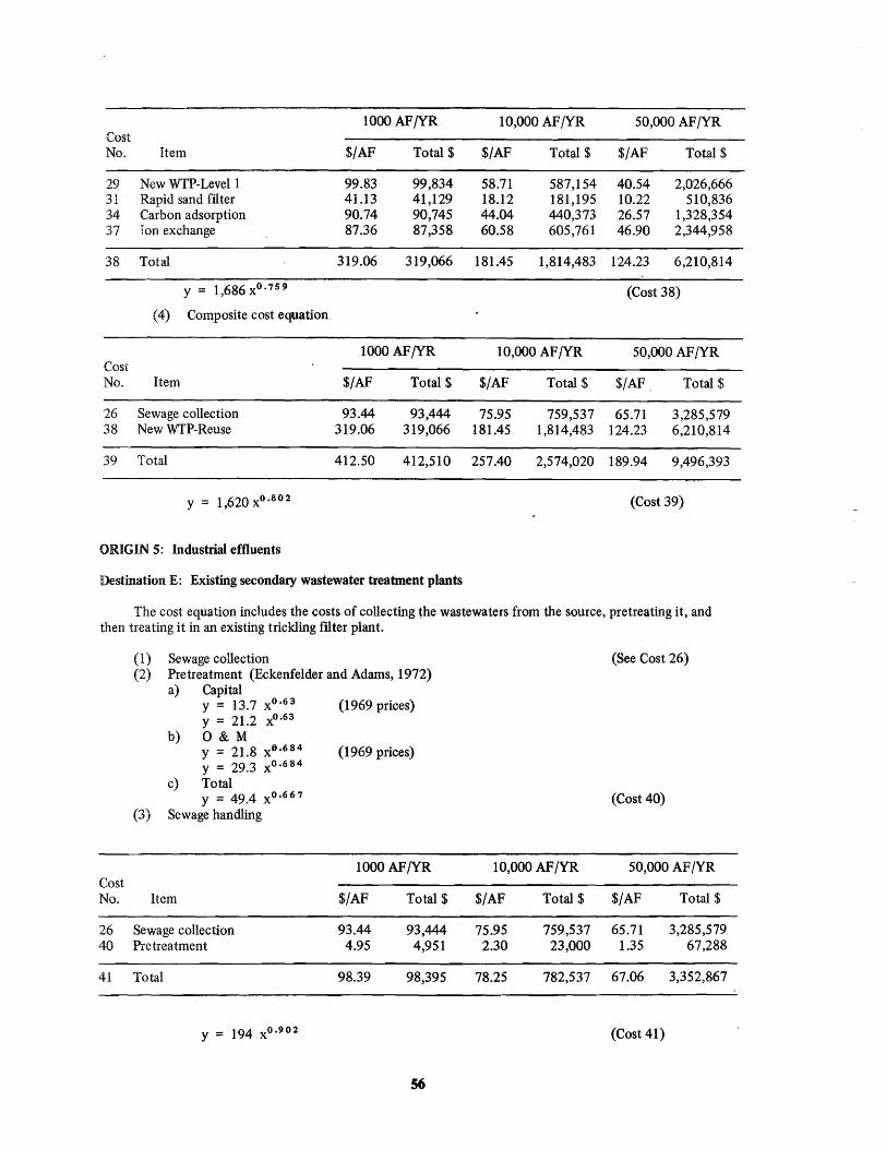
1000 AF/yR 10,000 AF /YR 50,000 AF/YR Cost No. Item $/AF Total $ $/AF Total $ $/AF Total $
29 New WTP-Level 1 99.83 99,834 58.71 587,154 40.54 2,026,666 31 Rapid sand filter 41.13 41,129 18.12 181,195 10.22 510,836 34 Carbon adsorption 90.74 90,745 44.04 440,373 26.57 1,328,354 37 Ion exchange 87.36 87,358 60.58 605,761 46.90 2,344,958
38 Total 319.06 319,066 181.45 1,814,483 124.23 6,210,814
y = 1,686 XO. 7S9 (Cost 38)
(4) Composite cost equation.
1000 AF/YR 10,000 AF/YR 50,000 AF /YR Cost No. Item $/AF Total $ $/AF Total $ $/AF. Total $
26 Sewage collection 93.44 93,444 75.95 759,537 65.71 3,285,579 38 New WTP-Reuse 319.06 319,066 181.45 1,814,483 124.23 6,210,814
39 Total 412.50 412,510 257.40 2,574,020 189.94 9,496,393
y = 1,620 XO.802 (Cost 39)
ORIGIN 5: Industrial effluents
Destination E: Existing secondary wastewater treatment plants
The cost equation includes the costs of collecting the wastewaters from the source, pretreating it, and then treating it in an existing trickling ftlter plant.
(1) Sewage collection (See Cost 26) (2) Pretreatment (Eckenfelder and Adams, 1972)
a) Capital y = 13.7 XO. 63 (1969 prices) y = 21.2 XO.63
b) 0 & M y = 21.8 X O•
684 (1969 prices) y = 29.3 XO. 684
c) Total y = 49.4 xO.667 (Cost 40)
(3) Sewage handling
1000 AF/YR 10,000 AF /YR 50,000 AF /YR Cost No. Item $/AF Total $ $/AF Total $ $/AF Total $
26 Sewage collection 93.44 93,444 75.95 759,537 65.71 3,285,579 40 Pre trea tmen t 4.95 4,951 2.30 23,000 1.35 67,288
41 Total 98.39 98,395 78.25 782,537 67.06 3,352,867
y = 194 XO.902 (Cost 41)
56
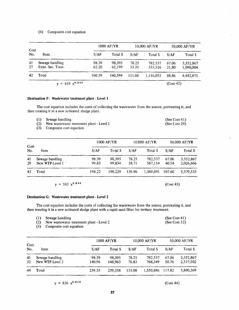
(4) Composite cost equation
1000 AF/YR 10,000 AF/YR 50,000 AF/YR Cost No. Item $/AF Total $ $/AF Total $ $/AF Total $
41 Sewage handling 98.39 98,395 78.25 782,537 67.06 3,352,867 27 Exist. Sec. Treat. 62.20 62,199 33.35 333,516 21.80 1,090,004
42 Total 160.59 160,594 111.60 1,116,053 88.86 4,442,871
y = 459 XO.848 (Cost 42)
Destination F: Wastewater treatment plant - Levell
The cost equation includes the costs of collecting the wastewater from the source, pretreating it, and then treating it in a new activated sludge plant.
Cost No.
41 29
43
(1) Sewage handling (2) New wastewater treatment plant - Levell (3) Composite cost equation
1000 AF/YR
Item $/AF Total $
Sewage handling 98.39 98,395 New WTP-Level 1 99.83 99,834
Total 198.22 198,229
y = 583 XO.844
Destination G: Wastewater treatment plant - Level 2
10;000 AF /YR
$/AF Total $
78.25 782,537 58.71 587,154
136.96 1,369,691
(See Cost 41) (See Cost 29)
50,000 AF/YR
$/AF Total $
67.06 3,352,867 40.54 2,026,666
107.60 5,379,533
(Cost 43)
The cost equation includes the costs of collecting the wastewater from the source, pretreating it, and then treating it in a new activated sludge plant with a rapid sand filter for tertiary treatment.
Cost No.
41 32
44
(1 ) Sewage handling (2) New wastewater treatment plant - Level 2 (3) Composite cost equation
1000 AF/YR
Item $/AF Total $
Sewage handling 98.39 98,395 New WTP-Level 2 140.96 140,963
Total 239.35 239,358
y = 836 X O•8 1 9
57
10,000 AF/YR
$/AF Total $
78.25 782,537 76.83 768,349
155.08 1,550,886
(See Cost 41 ) (See Cost 32)
50,000 AF/YR
$/AF Total $
67.06 3,352,867 50.76 2,537,502
117.82 5,890,369
(Cost 44)
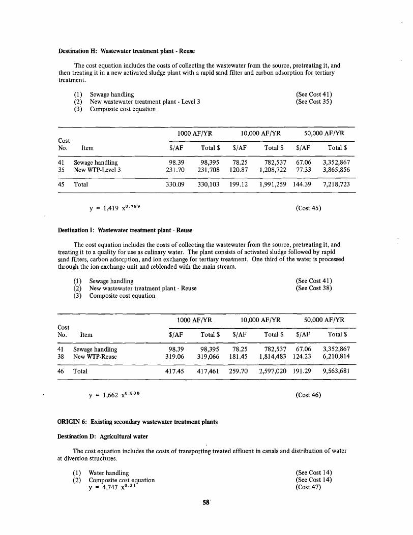
Destination H: Wastewater treatment plant - Reuse
The cost equation includes the costs of collecting the wastewater from the source, pretreating it, and then treating it in a new activated sludge plant with a rapid sand filter and carbon adsorption for tertiary treatment.
Cost No.
41 35
45
(1) Sewage handling (2) New wastewater treatment plant - Level 3 (3) Composite cost equation
1000 AF/YR
Item $/AF Total $
Sewage handling 98.39 98,395 New WTP-Level 3 231.70 231,708
Total 330.09 330,103
y = 1,419 XO. 789
Destination I: Wastewater treatment plant - Reuse
10,000 AF/YR
$/AF Total $
78.25 782,537 120.87 1,208,722
199.12 1,991,259
(See Cost 41) (See Cost 35)
50,000 AF/YR
$/AF Total $
67.06 3,352,867 77.33 3,865,856
144.39 7,218,723
(Cost 45)
The cost equation includes the costs of collecting the wastewater (rom the source, pretreating it, and treating it to a quality for use as culinary water. The plant consists of activated sludge followed by rapid sand mters, carbon adsorption, and ion exchange for tertiary treatment. One third of the water is processed through the ion exchange unit and reblended with the main stream.
(1) Sewage handIing (2) New wastewater treatment plant - Reuse (3) Composite cost equation
1000 AF/YR Cost No. Item $/AF Total $
41 Sewage handling 98.39 98,395 38 New WTP-Reuse 319.06 319,066
46 Total 417.45 417,461
y = 1,662 XO•8OO
ORIGIN 6: Existing secondary wastewater treatment plants
Destination D: Agricultural water
10,000 AF/YR
$/AF Total $
78.25 782,537 181.45 1,814,483
259.70 2,597,020
(See Cost 41) (See Cost 38)
50,000 AF /YR
$/AF Total $
67.06 3,352,867 124.23 6,210,814
191.29 9,563,681
(Cost 46)
The cost equation includes the costs of transporting treated effluent in canals and distribution of water at diversion structures.
(1) Water handling (2) Composite cost equation
y = 4,747 X O •31
58'
(See Cost 14) (See Cost 14) (Cost 47)
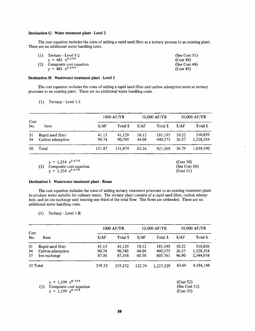
Destination G: Water treatment plant - Level 2
The cost equation includes the costs of adding a rapid sand ftlter as a tertiary process to an existing plant. There are no additional water handling costs.
(1)
(2)
Tertiary - Level 1-2 y = 481 XO. 644
Composite cost equation y = 481 XO.644
Destination H: Wastewater treatment plant - Level 3
(See Cost 31) (Cost 48) (See Cost 48) (Cost 49)
The cost equation includes the costs of adding a rapid sand ftlter and carbon adsorption units as tertiary processes to an existing plant. There are no additional water handling costs.
Cost No.
31 34
50
(1) Tertiary - Level 1-3
Item
Rapid sand ftl ter Carbon adsorption
Total
(2) y = 1,254 XO. 674
Composite cost equation y = 1,254 XO •6 74
1000 AF/YR
$/AF Total $
41.13 41,129 90.74 90,745
131.87 131,874
Destination I: Wastewater treatment plant - Reuse
10,000 AF/YR 50,000 AF/YR
$/AF Total $ $/AF Total $
18.12 181,195 10.22 510,836 44.04 440,373 26.57 1,328,354
62.16, 621,568 36.79 1,839,190
(Cost 50) (See Cost 50) (Cost 51)
The cost equation includes the costs of adding tertiary treatment processes to an existing treatment plant to produce water suitable for culinary water. The tertiary plant consists of a rapid sand filter, carbon adsorption, and an ion exchange unit treating one third of the total flow. The flows are reblended. There are no additional water handling costs.
(1) Tertiary - Level1-R
Cost No. Item
31 Rapid sand filter 34 Carbon adsorption 37 Ion exchange
52 Total
y = 1,199 XO. 754
(2) Composite cost equation y = 1,199 XO. 754
1000 AF/YR
$/AF Total $
41.13 41,129 90.74 90,745 87.36 87,358
219.23 219,232
59
10,000 AF/YR 50,000 AF/YR
$/AF Total $ $/AF Total $
18.12 181,195 10.22 510,836 44.04 440,373 26.57 1,328,354 60.58 605,761 46.90 2,344,958
122.74 1,227,329 83.69 4,184,148
(Cost 52) (See Cost 52) (Cost 53)

ORIGIN 7: Wastewater treatment - Levell
Destination D: Agricultural water
The cost equation includes the costs of transporting the treated effluent from a new activated plant and distributing the water at diversion structures.
(1) Water handling (2) Composite cost equation
y = 4,747 XO. 31
Destination G: Wastewater treatment - Level 2
(See Cost 14) (See Cost 14) (Cost 54)
The cost equation includes the costs of adding a rapid sand filter as a tertiary treatment process to a new activated sludge treatment plant. The costs were increased 5 percent to force the use of the existing secondary treatment plants over the construction of new ones. There are no additional water handling costs.
(1) Tertiary - Level N-2 y = 481 XO. 644
Y = 505 XO. 644
(2) Composite cost equation
y = 505 XO. 644
Destination H: Wastewater treatment plant - Level 3
(See Cost 31) (Cost 55) (See Cost 55)
(Cost 56)
The cost equation includes the costs of adding a rapid sand filter and carbon adsorption units as tertiary processes to a new activated sludge plant. The costs were increased 5 percent to force the use of the existing secondary treatment plants over the construction of new ones. There are no additional water handling costs.
(1) Carbon adsorption y = 794 XO. 686
Y = 834 XO. 686
(2) Tertiary - Level N-3 y = 1,254 XO. 674
Y = 1,317 XO. 674
(3) Composite cost equation y = 1,317 X O•6 74
Destination I: Wastewater treatment plant - Reuse
(See Cost 34) (Cost 57)
(See Cost 50) (Cost 58) (See Cost 58) (Cost 59)
the cost equation includes the costs of adding tertiary treatment processes to a new activated sludge plant to produce water suitable for culinary use. The tertiary treatment consists of rapid sand ftlter, carbon adsorption, and ion exchange units. The ion exchange units process one third of the total water flow and then blend with main stream. The costs were increased 5 percent to force the use of the existing treatment plants over the construction of new ones. There are no additional water handling costs.
(1)
(2)
(3)
Ion exchange (33% blend) y = 262 XO. 841
Y = 275 XO. 841
Tertiary - Level N-R y = 1,199 XO. 7S ·4
Y = 1,259 xO • 7 54
Composite cost equation y = 1,259 XO. 7S4
60
(See Cost 37) (Cost 60)
(See Cost 52) (Cost 61) (See Cost 61) (Cost 62)
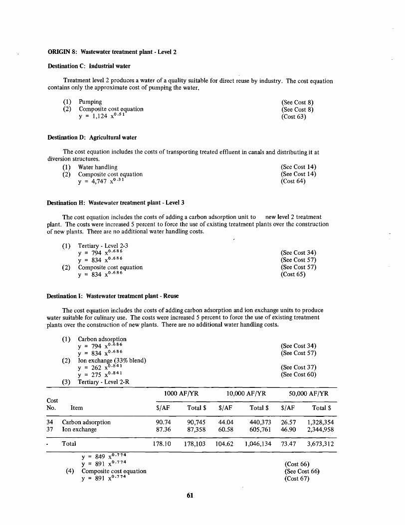
ORIGIN 8: Wastewater treatment plant - Level 2
Destination C: Industrial water
Treatment level 2 produces a water of a quality suitable for direct reuse by industry. The cost equation contains only the approximate cost of pumping the water.
(1) Pumping (2) Composite cost equation
y = 1,124 XO. 51
Destination D: Agricultural water
(See Cost 8) (See Cost 8) (Cost 63)
The cost equation includes the costs of transporting treated effluent in canals and distributing it at diversion structures.
(1) Water handling (2) Composite cost equation
y = 4,747 XO. 31
Destination H: Wastewater treatment plant - Level 3
(See Cost 14) (See Cost 14) (Cost 64)
The cost equation includes the costs 0f adding a carbon adsorption unit to new level 2 treatment plant. The costs were increased 5 percent to force the use of existing treatment plants over the construction of new plants. There are no additional water handling costs.
(1)
(2)
Tertiary - Level 2-3 y = 794 XO. 686
Y = 834 XO. 686
Composite cost equation y = 834 XO. 686
Destination I: Wastewater treatment plant - Reuse
(See Cost 34) (See Cost 57) (See Cost 57) (Cost 65)
The cost equation includes the costs of adding carbon adsorption and ion exchange units to produce water suitable for culinary use. The costs were increased 5 percent to force the use of existing treatment plants over the construction of new plants. There are no additional water handling costs.
(1)
(2)
(3)
Cost
Carbon adsorption y = 794 xO.686
Y = 834 XO. 686
Ion exchange (33% blend) y = 262 XO. 841
Y = 275 XO.841
Tertiary - Level 2-R
No. Item
34 Carbon adsorption 37 Ion exchange
1000 AF/YR
$/AF
90.74 87.36
Total $
90,745 87,358
Total 178.10 178,103
y = 849 XO. 774
Y = 891 XO. 774
(4) Composite cost equation y = 891 XO. 774
61
10,000 AF/YR
$/AF Total $
44.04 440,373 60.58 605,761
104.62 1,046,134
(See Cost 34) (See Cost 57)
(See Cost 37) (See Cost 60)
50,000 AF /YR
$/AF Total $
26.57 1,328,354 46.90 2,344,958
73.47 3,673,312
(Cost 66) (See Cost 66) (Cost 67)

ORIGIN 9: Wastewater treatment plant - Level 3
Destination A: Water treatment plants
The cost equation includes the costs of a pipeline and pump for the transmis.sion of treated effluent to the water treatment plants.
(1) Constraints a) Pipe line length - 8 miles b) Pump lift - 1000 feet c) Pump efficiency - 0.092 d) Power cost - $0.02/kw-hr
(2) Pipelines (1970 prices, Bishop et aI., 1974, p. 44)
The cost equation for the pipeline includes the annual capital and 0 & M costs, and also the cost of pumping necessary to overcome headloss. It does not include the cost of pumping to change elevation. The equation is based on the following values:
Slope = 2 ft/ 1 000 ft, down hill Power = $0.02/kw-hr Efficiency = 0.92 C = 120
It was assumed that capital repayment accounted for 75 percent of the total annual payment.
a) Capital y = 134 XO.5 35 $/mi (1970 prices) y = 193 XO.5 35 ${mi y = 1,544 XO.5 35 $/8 mi
b) 0 & M y = 45.0 xO.'535 $/mi (1970 prices) y = 56.0 XO. 5 3 5 $/mi y = 448 XO. 535 $/8 mi
c) Total y = 179 XO. 535 $/mi (1970 prices) y = 249 XO. 5 35 $/mi y = 1,992 XO. 535 $/8mi
(3) Pumping (Dawes, 1970, Figure 12) (Cost 68)
It was assumed that the pumps included with the pipeline are adequate to pump to the required heads. Therefore, only the cost of power required to pump the required heads are included in this section. An economy of scale of 0.90 was used to account for power rate charts.
a) 0 & M
3.148 H XO. 90 P y = Eo
where y = dollars H ~ feet of pump lift x = AF/YR P = Price of power, $0.02/kw-hr Eo = Pump efficiency, 0.92
y = 0.0684 H XO.90
for H = 1000 ft y = 68.4 XO. 90
b) Total y = 68.4 XO. 90
(4) Water transmission
61
(Cost 69)
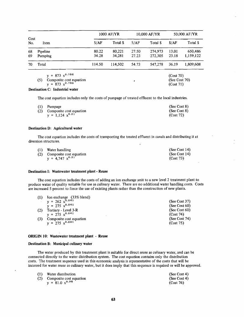
1000 AF/YR 10,000 AF/YR 50,000 AF/YR Cost No. Item $/AF Total $ $/AF Total $ $/AF Total $
68 Pipeline 80.22 80,221 27.50 274,973 13.01 650,486 69 Pumping 34.28 34,281 27.23 272,305 23.18 1,159,122
70 Total 114.50 114,502 54.73 547,278 36.19 1,809,608
y = 873 XO. 706 (Cost 70) (5) Composite cost equation (See Cost 70)
y = 873 xO. 706 (Cost 71) Destination C: Industrial water
The cost equation includes only the costs of pumpage of treated effluent to the local industries.
(1) Pumpage (2) Composite cost equation
y = 1,124 XO. S1
Destination D: Agricultural water
(See Cost 8) (See Cost 8) (Cost 72)
The cost equation includes the costs of transporting the treated effluent in canals and distributing it at diversion structures.
(1) (2)
Water handling Composite cost equation y = 4,747 XO. 31
Destination I: Wastewater treatment plant - Reuse
(See Cost 14) (See Cost 14) (Cost 73)
The cost equation includes the costs of adding an ion exchange .unit to a new level 2 treatment plant to produce water of quality suitable for use as culinary water. There are no additional water handling costs. Costs are increased 5 percent to force the use of existing plants rather than the construction of new plants.
(1)
(2)
(3)
Ion exchange (33% blend) y = 262 XO.8 41
Y = 275 XO. 841
Tertiary - Level 3-R y = 275 XO.841
Composite cost equation y = 275 XO.841
ORIGIN 10: Wastewater treatment plant - Reuse
Destination B: Municipal culinary water
(See Cost 37) (See Cost 60) (See Cost 60) (Cost 74) (See Cost 74) (Cost 75)
The water produced by this treatment plant is suitable for direct reuse as culinary water, and can be connected directly to the water distribution system. The cost equation contains only the distribution costs. The treatment sequence used in this economic analysis is representative of the costs that will be incurred for water reuse as culinary water, but it does imply that this sequence is required or will be approved.
(1) Water distribution (2) Composite cost equation
y = 81.0 XO.90
63
(See Cost 4) (See Cost 4) (Cost 76)
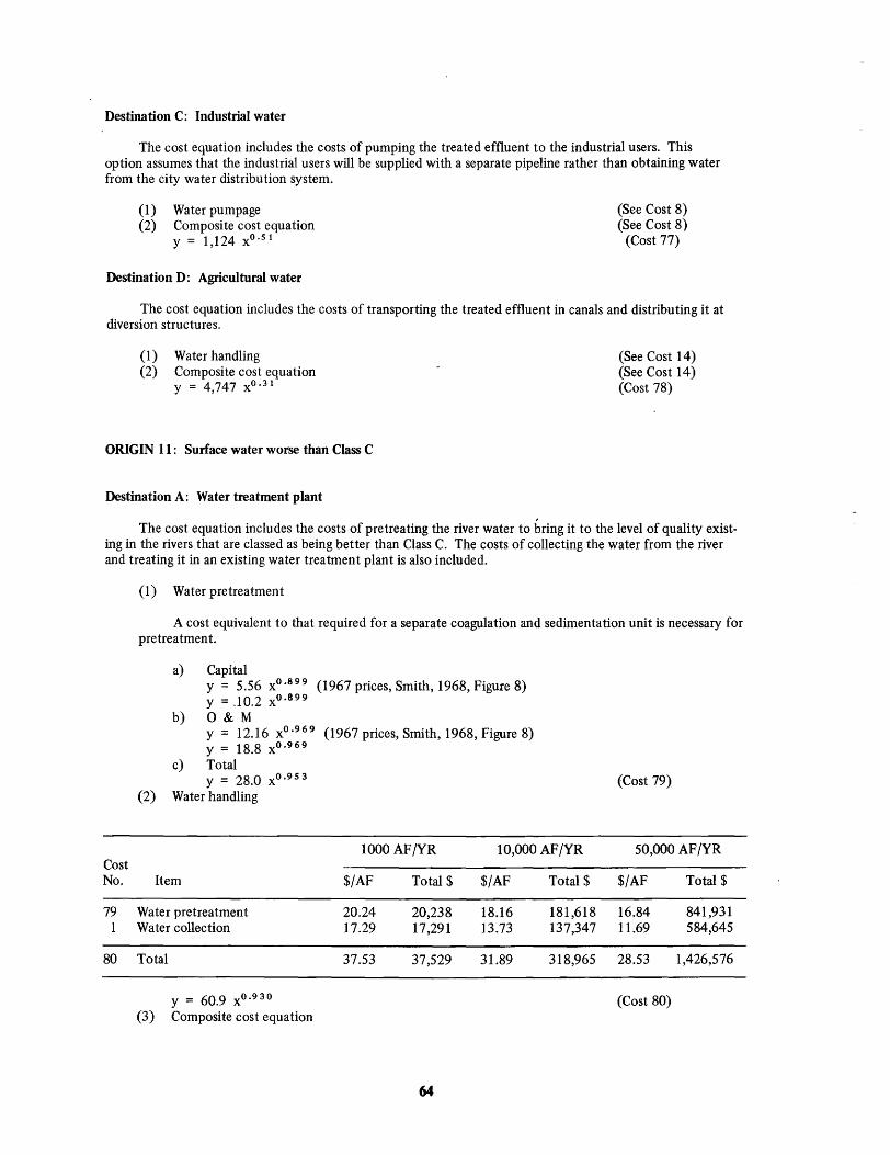
Destination C: Industrial water
The cost equation includes the costs of pumping the treated effluent to the industrial users. This option assumes that the industrial users will be supplied with a separate pipeline rather than obtaining water from the city water distribution system.
(1) Water pumpage (2) Composite cost equation
y = 1,124 xo.s 1
Destination D: Agricultural water
(See Cost 8) (See Cost 8)
(Cost 77)
The cost equation includes the costs of transporting the treated effluent in canals and distributing it at diversion structures.
(1) Water handling (2) Composite cost equation
y = 4,747 XO
.31
ORIGIN 11: Surface water worse than Class C
Destination A: Water treatment plant
(See Cost 14) (See Cost 14) (Cost 78)
The cost equation includes the costs of pretreating the river water to bring it to the level of quality existing in the rivers that are classed as being better than Class C. The costs of collecting the water from the river and treating it in an existing water treatment plant is also included.
Cost No.
79 1
80
(1) Water pretreatment
A cost equivalent to that required for a separate coagulation and sedimentation unit is necessary for pre trea tmen t.
a) Capital y = 5.56 XO.
899 (1967 prices, Smith, 1968, Figure 8) y = JO.2 XO. 899
b) 0 & M y = 12.16 XO. 9 6 9 (1967 prices, Smith, 1968, Figure 8) y = 18.8 XO. 969
c) Total y = 28.0 XO. 953
(2) Water handling
1000 AF/YR 10,000 AF /YR
Item $/AF Total $ $/AF Total $
Water pretreatment 20.24 20,238 18.16 181,618 Water collection 17.29 17,291 ]3.73 137,347
Total 37.53 37,529 31.89 318,965
Y = 60.9 XO. 93O
(3) Composite cost equation
64
(Cost 79)
50,000 AF/YR
$/AF Total $
16.84 841,931 11.69 584,645
28.53 1,426,576
(Cost 80)
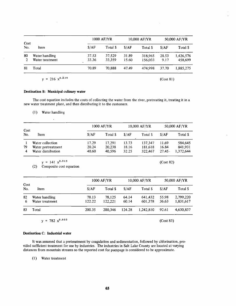
1000 AF/YR 10,000 AF /YR 50,000 AF /YR Cost No. Item $/AF Total $ $/AF Total $ $/AF Total $
80 Water handling 37.53 37,529 31.89 318,965 28.53 1,426,576 2 Water treatment 33.36 33,359 15.60 156,033 9.17 458,699
81 Total 70.89 70,888 47.49 474,998 37.70 1,885,275
y = 216 XO. S39 (Cost 81)
Destination B: Municipal culinary water
The cost equation includes the costs of collecting the water from the river, pretreating it, treating it in a new water treatment plant, and then distributing it to the customers.
(1) Water handling
1000 AF/YR 10,000 AF/YR 50,000 AF/YR Cost No. Item $/AF Total $ $/AF Total $ $/AF Total $
1 Water collection 17.29 17,291 13.73 137,347 11.69 584,645 79 Water pretreatment 20.24 20,238 18.16 181,618 16.84 841,931 4 Water distribution 40.60 40,596 32.25 322,467 27.45· 1,372,644
y = 141 XO. 915 (Cost 82) (2) Composite cost equation
1000 AF/YR 10,000 AF/YR 50,000 AF /YR Cost No. Item $/AF Total $ $/AF Total $ $/AF Total $
82 Water handling 78.13 78,125 64.14 641,432 55.98 2,799,220 6 Water treatment 122.22 122,221 60.14 601,378 36.63 1,831,617
83 Total 200.35 200,346 124.28 1,242,810 92.61 4,630,837
y = 782 XO. S03 (Cost 83)
Destination C: Industrial water
It was assumed that a pretreatment by coagulation and sedimentation, followed by chlorination, provided sufficient treatment for use by industries. The industries in Salt Lake County are located at varying distances from mountain streams so the reported cost for pUl,llpage is considered to be approximate.
(1) Water treatment
6S
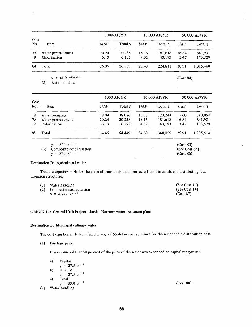
1000,AF/YR 10,000 AF/YR 50,000 AF /YR Cost No. Item $/AF Total $ $/AF Total $ $/AF Total $
79 Water pretreatment 20.24 20,238 18.16 181,618 16.84 841,931 9 Chlorination 6.13 6,125 4.32 43,193 3.47 173,529
84 Total 26.37 26,363 22.48 224,811 20.31 1,015,460
y = 41.9 XO. 933 (Cost 84) (2) Water handling
1000 AF/YR 10,000 AF/YR 50,000 AF /YR Cost No. Item $/AF Total $ $/AF Total $ $/AF Total $
8 Water pumpage 38.09 38,086 12.32 123,244 5.60 280,054 79 Water pretreatment 20.24 20,238 18.16 181,618 16.84 841,931 9 Chl orina tion 6.13 6,125 4.32 43,193 3.47 173,529
85 Total 64.46 64,449 34.80 348,055 25.91 1,295,514
y = 322 XO. 767 (Cost 85) (3) Composite cost equation (See Cost 85)
y = 322 xO. 7 6 7 (Cost 86)
Destination D: Agricultural water
The cost equation includes the costs of transporting the treated effluent in canals and distributing it at diversion structures.
(1) Water handling (2) Composite cost equation
y = 4,747 XO. 31
ORIGIN 12: Central Utah Project - Jordan Narrows water treatment plant
Destination B: Municipal culinary water
(See Cost 14) (See Cost 14) (Cost 87)
The cost equation includes a ftxed charge of 55 dollars per acre-foot for the water and a distribution cost.
(1) Purchase price
It was assumed that 50 percent of the price of the water was expended on capital repayment.
a) Capital y = 27.5 x1.0
b) O&M y = 27.5 x1.0
c) Total y = 55.0 x
1•O (Cost 88)
(2) Water handling
66
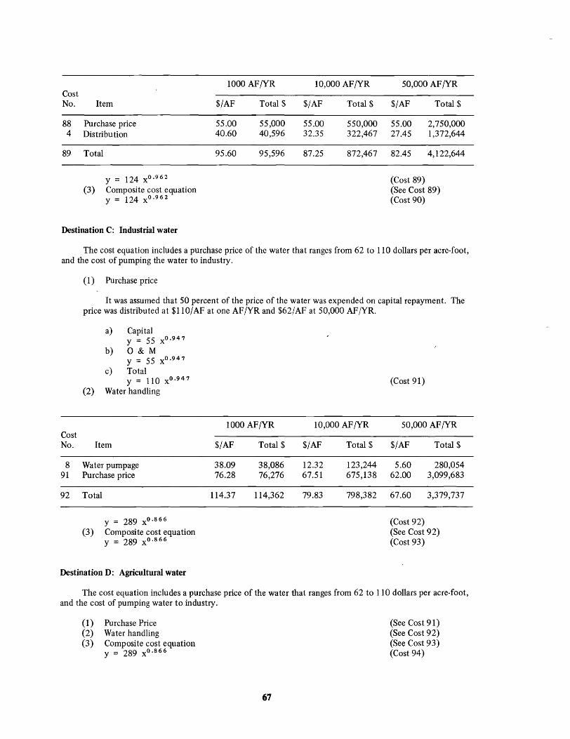
Cost No. Item
88 Purchase price 4 Distribution
89 Total
y = 124 XO. 962
(3) Composite cost equation y = 124 X O. 9 6 2
Destination C: Industrial water
1000 AF/YR
$/AF
55.00 40.60
95.60
Total $
55,000 40,596
95,596
10,000 AF /YR
$/AF
55.00 32.35
87.25
Total $
550,000 322,467
872,467
50,000 AF /YR
$/AF Total $
55.00 2,750,000 27.45 1,372,644
82.45 4,122,644
(Cost 89) (See Cost 89) (Cost 90)
The cost equation includes a purchase price of the water that ranges from 62 to 110 dollars per acre-foot, and the cost of pumping the water to industry.
Cost No.
8 91
92
(1 ) Purchase price
It was assumed that 50 percent of the price of the water was expended on capital repayment. The price was distributed at $110/AF at one AF/YR and $62/AF at 50,000 AF/YR.
a) Capital y = 55 XO. 947
b) O&M y = 55 XO. 947
c) Total y = 110 XO. 947 (Cost 91)
(2) Water handling
1000 AF/YR 10,000 AF/YR 50,000 AF/YR
Item $/AF Total $ $/AF Total $ $/AF Total $
Water pumpage 38.09 38,086 12.32 123,244 5.60 280,054 Purchase price 76.28 76,276 67.51 675,138 62.00 3,099,683
Total 114.37 114,362 79.83 798,382 67.60 3,379,737
y = 289 XO. 866 (Cost 92) (3) Composite cost equation (See Cost 92)
y = 289 XO. 866 (Cost 93)
Destination D: Agricultural water
The cost equation includes a purchase price of the water that ranges from 62 to 110 dollars per acre-foot, and the cost of pumping water to industry.
(1) Purchase Price (2) Water handling (3) Composite cost equation
y = 289 XO. 866
67
(See Cost 91) (See Cost 92) (See Cost 93) (Cost 94)
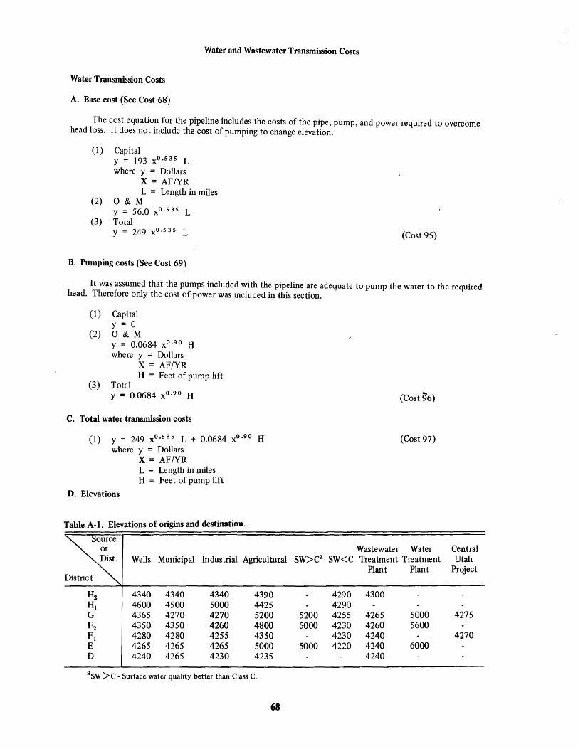
Water and Wastewater Transmission Costs
Water Transmission Costs
A. Base cost (See Cost 68)
The cost equation for the pipeline includes the costs of the pipe, pump, and power required to overcome head loss. It does not include the cost of pumping to change elevation.
(1) Capital y = 193 XO. 5 35 L where y = Dollars
X = AFjYR L = Length in miles
(2) 0 & M y = 56.0 XO. 535 L
(3) Total y = 249 XO. 535 L
B. Pumping costs (See Cost 69)
(Cost 95)
It was assumed that the pumps included with the pipeline are adequate to pump the water to the required head. Therefore only the cost of power was included in this section.
(1) Capital y = 0
(2) 0 & M y = 0.0684 XO. 90 H where y = Dollars
X = AFjYR H = Feet of pump lift
(3) Total y = 0.0684 XO. 90 H
C. Total water transmission costs
(1) y = 249 XO. 535 L + 0.0684 XO.90 H where y = Dollars
X = AFjYR L = Length in miles H = Feet of pump lift
D. Elevations
Table A-I. Elevations of origins and destination.
or Dist. Wells Municipal Industrial Agricultural SW>Ca
District
H2 4340 4340 4340 4390 HI 4600 4500 5000 4425 G 4365 4270 4270 5200 5200 F2 4350 4350 4260 4800 5000 FI 4280 4280 4255 4350 E 4265 4265 4265 5000 5000 D 4240 4265 4230 4235
aSw >C - Surface water quality better than Class C.
68
(Cost 96)
(Cost 97)
Wastewater Water Central SW<C Treatment Treatment Utah
Plant Plant Project
4290 4300 4290 4255 4265 5000 4275 4230 4260 5600 4230 4240 4270 4220 4240 6000
4240
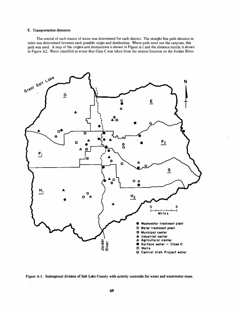
E. Transportation distances
The central of each source of water was determined for each district. The straight line path distance in miles was determined between each possible origin and destination. Where path must run the canyons, this path was used. A map of the origins and destinations is shown in Figure A-I and the distance matrix is shown in Figure A-2. Water classified as worse that Class C was taken from the nearest location on the Jordan River.
o Water treatment plant o Municipal center • Industrial center b. AQricultural center • Surface water - Class C C Wells
N
~
e Central Utah Project water
Figure A-I. Subregional division of Salt Lake County with activity centroids for water and wastewater reuse.
69
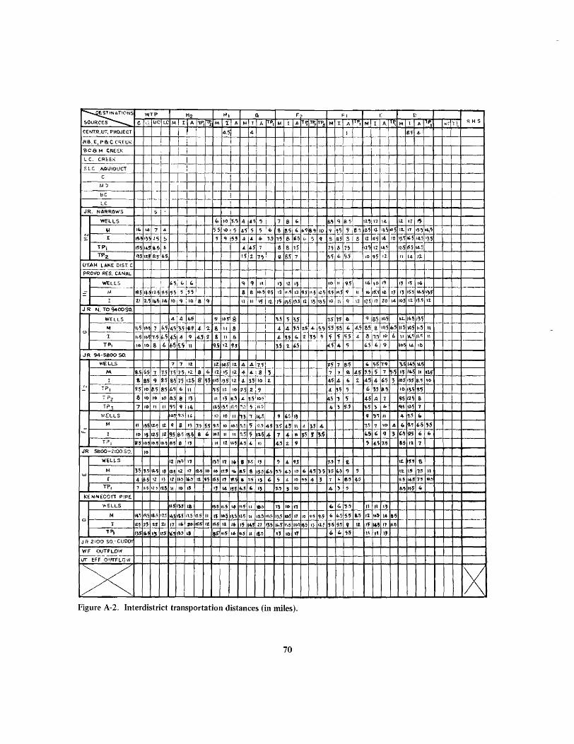
~s WTP H2 HI G F FI E D &OURCES c. ., IJC LC M, qA "tFjrrPz M 1: A M r /. TPI 104 I A TP' W, iP3 M I A P, M I AI~ M I ""Pl ¥-t'J ~ ~ RHS
CENTR.UT, PROJECT I 4.~ 4 I 8·5 4-
RB,E,PS.CC,,\EE" I i : i
SCa.M CREEK 1 i ! I I L C. CREE." ------- ! I
SLC A.<lUIOUCT 1 ! I
C I '-l-f-- I- '=--1 - I - 1--I-M:) =-H- I
.--
llC .. - ~- --
I I
~- I
! , - -I--iT --f-T LC I JR. NARROwS ':i I- I i
WELLS b 10 15.') 4 ./i r;j 7 8 " So, q 85 11',) 12 \4- 12. 17 ,0; - - ._-
'" II:. 14 7 4 5.5 10 j OJ
40; " 'j ~ S !S , 6'18·Q 10 9 '15 9 8·'1 11·'5 Il. 'l~ IO~ IL 11 '5·') 14,'i
N I 1t;.~ll!i 5 q i'" A. " M 15 1'5 !;) 4 ~ '.r; " ~ q 9 85 3 II Il ,/., 14- 10 Ij.~ IH 145 ,}.r;
TP, 6'; 14' a.!l & .4, 7 I 8 8 1.5 H 8 7.~ \1~ 12 14.7 12·56·5 \4.5" f--=.-
7"J 1 -.-f-- --I-i-- . --I-f--
TP2 i"~ It.' 8.,. 1.5 ,.~ 2. e 8.'i 7 'j~ b ,.7 10 9') ,z. 1\ 14- 1'2.
UTAH LAt<.E DIST. C .L ~-REs:ciNAL -- -t-f-- r-- --~-- -
I -'r- -'- I- - '. -- -
i WELLS ~~1-" " ~ q /1.1 r, 12. Il 10 " 'I'; 16 ,6 I~ I., ,'; I{,
----- _.- -- .. - - r-- -_ ... --- _. - 1-'- --M \HI~.1 11..~ 9.5 5~l5'i' 8 8 IO.~ 9.'j 1211.0; 110cH II-S 12.~ H IO.~ </ " 16 I'i.'j 18 fj I., 1')·5 \6.~ I~f - -. l 11 2.'i llo6 I. 10 q ; 10 8 9 11 II I, i 12. Ir; 1.,1) I'7J t1 I~ I}'"j 10 II 9 Ill. 17.5 11 ZO 14 10.' \, IH 11
JR N. TO 9400S0. ! WELLS 4~4 E.5 9 IOf 9 ! ~.~ ') ~ H ~:!. e q 1?'j iO.'j 11- 16.~ IH -- --r-- - -- ~.;.~ - '- - -- -- - 1--r-- .-- - --~ II·') IO.~ 7 f..') 8·, 4 '2. S H B I 4 4 ~.~ 1.·S, 4 '7'; 5!i 5!) l. 4..'7 8.'7 8 10.5 to.') \1·5 \4.5 II.'] 1\
<-'> ~514 +
'- T -a- f, ~-~ 1: II·~ ,b~ ,.0; 6:'.i 9 45 '1. 8 \I s _4:.. !.~- '" ~.~.'i r; Ii H 4- l;'i 10 " \4,<; --f- 1-- .. - I-- --- ----
TPI Ie. 10 8 (. h!jl5,7 II q.r; 11 H 3.'1 1- (,.'7 ~5 .4,- C; 6.5 (, 9 It> 104. It»
JR 94-5800 SO.
WELLS 7 7 It. Il. I4S )2- 4 AI7'!i- 7-r; 7 8~ ID r;·')ir q ~.~ 14~ II." --,- -7 ~.5 11 , .. ~ " ILf f--. '" '.'i~ .2_ M 7'i7-'7 12- 8 b 12 1'5 12 4- 4.18 ., 7 .., S 4~ ~.5 "
I & as 9 a·'i SIj 7.5 I1.S B "i.~ III/ IH 12 4- ~.'illo 1. -4,$ A- I":. 2. 4.746.7 } Ill!f fJ.f 8." 1O --,- TP, 2: 9 I "- 9.5 '0 8.5 8.5 6.<; (, 1\ 'is 11. 10 2·5 l H 5 (, ~.5 8.'7 10 I~~ 9.<;
8 I~ 1\.0; 4. 3.'iilo.~! --' - r--'
I P2 10 10 10 8.58 I., II 14·'7 "3 'i 4-S"A 1 1/.'; 12'i S
TP, 7 1O '\ 1\ 95 'I )4- 1Z,5 I~.~ 12.-5 ~:; I) : u-) 4- ~ ,.,. .,.OJ } 6 q~ \7.·5 7
wELLS o.'j'~.'j It. 10 10 II r-r.~ i llt.-~ 9 ,.~ I' 9 ")0; /I 41·5 (.
M II ,}.., 11..~ 11 q S ,~ 7·' H 9.~ 10 10.t; ~.; '7 '115 4-'i 7·<; 4·' 1\ .i 1.5 ~ l·~ '1 10 4 69.'1 ,.; 'j·5
..:: I '0 ,~ 12.;- 12 Ij'; 8·~ IH 8 " IO.~ \I " 7.'5" .~ I'I .. ~ 4- 7 4- II !, J ~~ (,5 , q } '!i 9.') (, 6 ---T"'I ~·1 10.' 10.Oj 10.' B·, 8 I, \I 1% I~' 4-, 04- " 4;5 2- 9 '; 4-,'; 1·5 &5 12 1
JR 5800-<.00 so. /0 I WELLS 12. '~7 11 1'j.5 17 ,(, 8 1.~
" ~ 4- 9.'i 1·' 1 i. It. ,., eo
/Ii 3.5 '1.511.') " 1M 12 .7 I'L-~ 10 '6 17.' I" as 8 ".~ ,-", ..... '.';i 4-.' 10 l. 4.'; ,·5 11.5 ,.~ q '} I"Z. IS" 15 " I 4 8·'1 '2 I~ 12 I~; 1'·~ I'Z. 9~ Is·S '7 1'1." & 1.'; I) , ? o!- 10 .,., 4 3 7 " 6·0; 4·7 u·S ,,,S 7'i fD.~
TP1 1 \I., '25 11.5 II 10 15 I' 14 I'~ 6.5 t. I} ~.'} , 10 4- ,15 a.r; ".'1 " I<ENNECOn P!PE
~::lLS I~~ l}of 18 ,., I\·S 1+ I\·f II ... .., 11 10 n " (" '.'1 II " I} -M I~~ \'1.~ 18.; '7.~ 14.$ll~ 11.~ 11.'7 II IJ lO~ IJ-S ".~ II 15.'1 10.~ 1}5 IG.~ 17 10 q.o; 9·~ (" 6.'} 0;.'1 ,"j 1'2. ,,!j ~ ~ 0 _.--- -_. ..... - --I 11·5 2S -1~ 2.1 17 16 lrD If.'> It. r;.'j " ,6 ,OJ '4.~ 22 ".~ 110.'5" I',.,} ·lD.~ .,.5 I} '1~ '1.5 'IS 9 11 )f f4.~ 11 'Ii
TPj 13SIt..5 ., 175 ",,}.7 II 15S' \I.S 14- 11.5 II IS·O; 11 ICI \1 " " 0;.'1 l\ "
I' JR 2100 SO.-CUOO'r
WF OUTFLOW -.--UT f:FF O'1TFI.O VI
X IX Figure A-2. Interdistrict transportation distances (in miles).
70
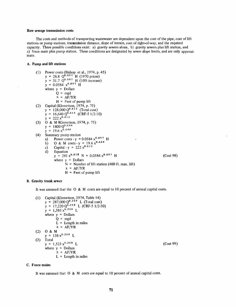
Raw sewage transmission costs
The costs and methods of transporting wastewater are dependent upon the cost of the pipe, cost of lift stations or pump stations, transmission distance, slope of terrain, cost of right-of-way, and the required capacity. Three possible conditions exist: a) gravity sewers alone, b) gravity sewers plus lift station, and c) force main plus pump station. These conditions are designated by sewer slope limits, and are only approximate.
A. Pump and lift stations
(1)
(2)
(3)
(4)
Power costs (Bishop et aI., 1974, p. 45) Y = 28.8 QO.897 H (1970 prices) y = 31.7 QO.897 H (10%increase) y = 0.0584 XO.897 H where y = Dollars
Q = mgd x = AF/YR H = Feet of pump lift
Capital (Klemetson, 1974, p. 75) Y = 128,000 QO.615 (Total cost) y = 16,640 QO .615 (CRF-5 1/2-10) Y = 222 XO .6 1 5 o & M (Klemetson, 1974, p. 75) Y = 1800 QO. 644
Y = 19.6 XO. 644
Summary pump station a) Power costs - y = 0.0584 xO.8 97 H b) 0 & M costs - Y = 19.6 XO.644
c) Capital - y = 222 XO.6 1 5 d) Equation
y = 241 xO.61S N + 0.0584xo.897 H where y = Dollars
N = Number of lift station (400 ft. max. lift) x = AF/YR H = Feet of pump lift
B. Gravity trunk sewer
(Cost 98)
It was assumed that the 0 & M costs are equal to 10 percent of annual capital costs.
(1)
(2)
(3)
Capital (Klemetson, 1974, Table 14) y = 287,000 QO.359 L (Total cost) y = 17,220 QO.359 L (CRF-5 1/2-50) y = 1,385 XO. 359 L where y = Dollars
Q = mgd L = Length in miles x = AF/YR
O&M y = 138xo.359 L Total y = 1,523 XO. 359 L where y = Dollars
x = AF/YR L = Length in miles
c. Force mains
It was assumed that 0 & M costs are equal to 10 percent of annual capital costs.
71
(Cost 99)
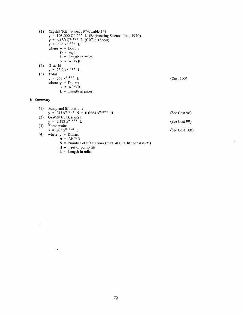
(1) Capital (Klemetson, 1974, Table 14) y = 103,000 QO.463 L (Engineering-Science, Inc., 1970) y = 6,180 QO.463 L (CRF-5 1/2-50)
(2)
(3)
y = 239 XO.463 L where y ::: Dollars
Q = mgd L = Length in miles x = AF/YR
O&M y = 23.9 XO. 463 L Total y = 263 Xo.4 63 L where y = Dollars
x = AF/YR L = Length in miles
D. Summary
(1) Pump and lift stations y = 241xo.618 N + 0.0584xo. 897 H
(2) Gravity trunk sewers y = 1,523xo.359 L
(3) Force mains y = 263 X°.463 L
(4) where y = Dollars x = AF/YR N = Number of lift stations (max. 400 f1. lift per statioh) H = Feet of pump lift L = Length in miles
72
(Cost 100)
(See Cost 98)
(See Cost 99)
(See Cost 100)
APPENDIXB
Optimal Solutions for the Various Model Formulations
73,


--..) CJI
'Tl 00' t: "'I (1)
9'
'" r (1) .... (') :::s o (1)
~~ ~ (') "'I 0 '< ~ -'" "'I ~
~ --..)
3~ rtl 0-- "'I
~~ o· ::i
~ :::s :::s t: e:.. 3 o 0.. ~
!. -=-0.. (I) -(I) "'I
3 5' ~.
~.
~ ~ -(I) "'I
~ <: ~. S' s: -iii' Vl
~
0.
~~ SOURCES CENTRAL UTAH PRO.l
RB, E, pac CREEKS BC a M CREEKS
lC CREEK SLC AQUEDUCT
C MD BC LC
JR NARROWS WELLS
M
;~ I
TFf T~
UTAH LAKE DIST. C PROVO RES. CANEL
WELLS
!HI M I
JR No to 9400 So. WELLS
G fA I
H'} JR 94-5800 So.
WELLS M
f2 I TP1
TP2 TP~
Wt.LlS
h=; M I
TP,
JR 5800-2100 SO.
I WELLS
EI M I
TP1
KENNECOTT PIPE WELLS
D M !
TPr U:--JTR EFF OUTFL'W
WF OlJTFLOW JR 2100 So -CUDAHY
ex
::><:: C MDBC LC
30.
~2.b
~3. B
14. 5
t-1"--'
0 <:> <:> <:>
1\1 N N 1\1
H2 HI G M I A TP, T~ M I A M I A TP,.~'
I ~_
5.8 I
22. 9 9.1 4.2 2'i7
42.1 90. S
4. 5
.2-
25.6
3.4
.8
2.1
.2
<;.6
I I
<:> <:> <:> <:> <:> <:> <:> <:> <:>
£ <:> <:> <:> <:> <:> <:> 0 <:> 00 N N '" '" 00 ~
~ 11'1 N ",' "," <:> N 11'1 on
'" a- N N N <:> 0 0 <:>
" " " N ~I " II _" " II II ~I "
F2 FI E 0 ~ X A Tf1 TPz m M I A TPr M I A TP' M I A TP. UT~WF JR RHS EF CD ~ 3 000
8.9 = U..l.Q.2. I ZOoS = 63 400
9.S = 1.1., 100
= 14.500
~ l'l 100
-+ 30.3 :S 35 900
-' 19.7 ~ 42.bOO 1 6.4 2.8 .1 ~ H2 100
1).5 15.1 18. I 35 ~ 206 300
~ 1 900
= 4 500
= ZOO 4.5 ~ 4 500
1.3 1.0 ~ 3 900
~ 25 600
- 3 400
~ 1 300
= 2.100
= a - -50. 5 = 50 500 (\.1 ~ B..l.Q.Q.
5.7 = 11.300
= a 4.6 1.0 ~ 5 600
37.'1 26.4 = 64 300
4 I s 4 600 -8.7 4.0 ~ 1~700
.3 = 300
~ 9 000
9 ~ 11...2.00
.-i ~ 5.100 - 2.1 ~ 2 100
7.1 = ~clQ.Q.
= a 7.\ ~ 7 800
2.Q I 5~! = iL3 jlJO
1.3 ~ 3~
24.R = 24 800
a2 = 8 200
'J ~ 50 40'1
Q.O; :s Q 500
24. 2 ~ .li.z.M
1.4 = 1 400
alB = 81 800
1.4 ~ 1 500 'I--
'4.2 = 24 200 , 06. = 166 200 I \.
87.5 i! 0
-.~-
~ g <:> 0 c ~ 0 0 0 0 0 0
<:> <:> 0 0 0 <:> 0 0 £ 0
'" 11'1 11'1 0 0 N a- GO l"- N
11'1 :!! .; on si N ,.; 0 on on
= 0 0 0 0 0 <:> 0 0 0 N 0
II " M M AI II " " AI " " II .1>L ~ ~t II 1\1 AI " 1\1
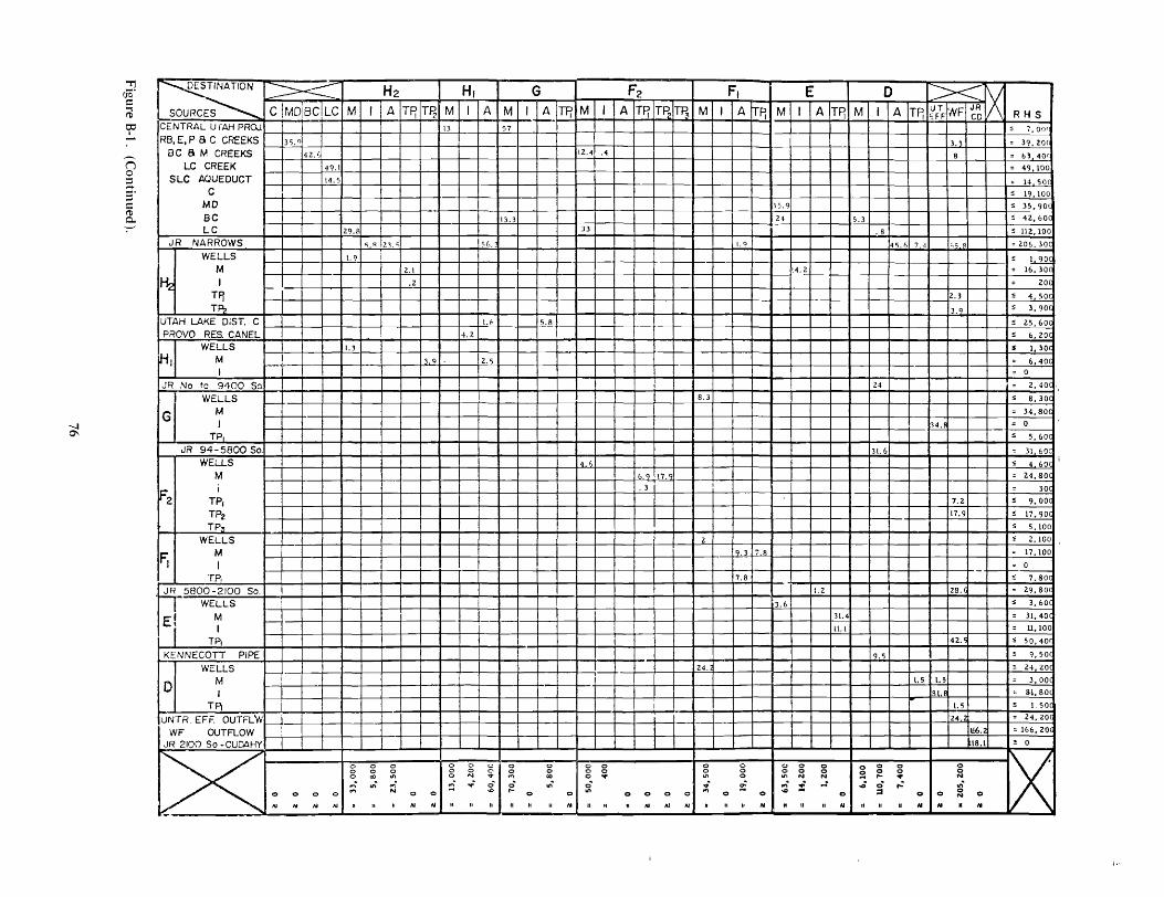
....... 0\
." 0'0' = '"'I (!l
~ .....
(j o -.... -,.... ;:c 0. --:--'
~ SOURCES CENTRAL UTAH PROJ. RB, E, pac CREEKS
DC a M CREEKS LC CREEK
SLC AQUEDUCT C
MD BC LC
JR NARROWS
WELLS M
~ I T~ T~
UTAH LAKE D'ST. C PROVO RES. CANEL
WELLS H, M
I JR No. to 9400 So.
WELLS
G M I
TP, JR 94-5800 So.
WELLS M
F: i 2 TP,
TPz TP:,!
WELLS
~ M I
"fP, JR ::>800 - 2100 So. "-r WELLS
E' M i I TP, KENNECOTT PIPE
WELLS
D M I
Tp!
UNTR. EFr-. OUTFLW WF OUTFLOW
JR 2100 So -CUDAHY
[X
~ C IMOBC LC
35. <)
42.r
49.1
14.5
-
I
0 0 0 0
1\1 1\1 1\1 1\1
H2 H, G M , A T~ TPz M , A M , A TP, M
13 57
12.4
13.3
29.8 33
~ '1 23. ~ 5 (, ..
1.9
2.1
.2
1.1- s.s 4.2
1.3
3,9 . Z.5
4. i)
0 0 0 0 0 0 0 0 0 0 0 0 0 0 c- o 0 0 0 co '" 0 N .q< .., co 0 ... on ..., .., ..... o· 0 '" o· ... N 0 0
-D ... 0 0 '"
" " " AI 1\1 H " " " " " AI "
F2 F, E 0 >< X I A TP' TPz m M I A TPr M I A TP. M I A TR UT 'NF JR RHS 'OFF CD :; 7.00'
l.~ = 39. lO[ .4 S = b 3 40 r
= 49,100
= 14 500 :5 19.100
\5.9 :5 35, qOl
24 5.l :5 42, bOe
.8 :5 lIZ.IOO
!.Q 45.6 7.~ ;<,8 = 206, loe
:5 1 90e 14.2 = 16. lOe
= 20(
2.3 :5 4 SOC
3.':L :5 3,90(
:5 25. bO(
:5 b. zoe
:s I, lOC
= 6,40(
= 0
24 = 2.40e
8.3 :5 8. lO(
= l4. SOC
34.f = 0 :5 5,60(
l\. 6 = 31 boe
:5 4 bO(
b.9 17.9 = 24, SO(
.3 I = 30(
7.2 :5 9, oDe
17.9 :5 17,90e
:5 5.100
2 s 2,100
9.3 7.8 = 17.100
= 0
7. B :5 7. soe
l.l. 28.£ = 29.S0(
3. b :5 3, bO(
31.4 = ll,40(
ILl = u,loa
42.' :5 50,40r
9.5 :5 9,sor
24. :5 24 lO[
1.5 1.5 = 3,OO[
SI.B .' SI, SO[
1.5 :5 1. SO[
24. = 24,201
lf6. = 166,201
\8.\ ~ 0
~ 0 0 0 0 0 0 0 0 0 0 0 0 0 0 0 0 2 0 0 0 .... '" 0 '" N N I"- .... N .... a- ... i .Q 0 r: on
0 0 0 0 ...
0 0 '" 0 ::I 0 0 0 0 N
" " 1\1 /oJ 1\1 " " " 1\1 II " " 1\1 " " u 1\1 1\1 I III
I·'
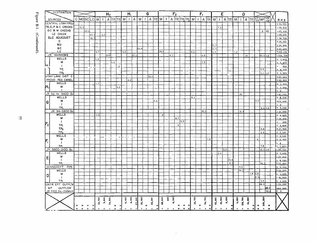
-...J -...J
"T1 00 :::: r:l t?
(j o ::;
§' (t) 0..
r--s:: SOURCES
CUHRAL UTAH PRQl
R8, E, P 8 C CREEKS
'8 CaM CREEKS LC CREEK
SLC AQUEDUCT C
MD Be LC
t-:iR NARROWS
J WELLS M
I
1 TP' TF\z
UTAH LAKE DIST. C PROVO RES CANEL
WELLS
HI M I
JR No to 9400 So WELLS
G M I
TP
JR 94-5800 So. WELLS
M
F'2 I
TP, TPz TP3
WELLS
Fj M I
TR J~ 5800-2100 SO.
WELLS
E M I
TP,
KENNECOTT PIPE
WELLS M 0 I
TF>!
UNTR. EFr OUTFL'W WF OUTFLOW
JR 2100 So.-CUMHY
~
~ C MDBC LC
31.'i
42. E
43.3
14. <;
1---
... - ...
...... -
0 a <;> 0
No No AJ /Il
H2 H, G M I A TP; T~ M I A M I A
S.B
26,9
6.7 6,4
3°.R 87.1
1.9
4.5
.2 r-1-- _.,
22.1
4.2
1.3
3.2
3.0
. -- .. _. '~r_ • U • . _-
0 0 0 0 0 <;> <;> 0 0 0 0 0 0
~ 0
~ '" 00 co ..,. N er-N Ill· ~ ,D .; r- oD N ~ .... 00 N N
a 0 a II II " /Il ~I II " It " " "
F2 F, E 0 ~ X T~ M I A T~ TR ~ M I A T"r~ M I A TP. M I A TF: ~:F WF ~~ RHS ;5 3b. 500
7.3 =39,2.00
.8 2.0 =63,400
= 49 100
= 14,500
~ 19 100
11. ~ ~ 35 ...2,00
15.7 ~ 42 .iL00 28. 6 H.4 4.5 1.2 ~ IlZ. 100
4.3 4.8 14 5.3 1.0 ;206 300
~ 1 900 ' 19 = 6,400 :
= 2.00 I
6.5 ~ 4 500 -2.6 1.0 ~ 3,900
" ~ 25 600
~ 40 000
~ .J 300
= 3 2.00
= a 46 = 46 000
8.3 ~ 8,300
5,6 7.7 =133 000
= 0
4.6 1.0 ~ 5,600
30.0 31.( = 61 000 .4 ~ 4 600
8.7 = 14 zoo 5.5 = 300
.3 ~~ 9.0 s 17 900
5.5 ~ 5 100
~ Z 100 ~
7.8 .5 ~ 8 300
= a 7.8 ~ 7 800
-~
Z.2 55.3 1.0 = 58 sao 3.6 s 3 600
=...z.s..~ 25.8 = !L ~
8. ~ 34.3 ~ 50 400
9.5 ~ 9 SOD
24.2 s 24 zoo 1.5 1.0 = 1 600
RI.B = 81 800
1.5 s 1. 500
4.2 = 24, lOa
I!i>.Z 3..b1:..2.llil. 90.1 ~ 0
~ 0 <;> <;> 0 0 0 0 0 0 0 0 0 0 0 0 0 0 a 0 a a a a a -.&> .. .... ,.. ,.. ... er- N N r- 0 N ,.; .; :2 oD ,.; 2 N ..; o· i on N .... on :1 a
a a a 0 a 0 a 0 0 N 0
N " " " H 1\1 N " " I, 1\1 " " " 1\1 11 " " 1\1 H " /If

-.....] 00
"Tl ric' e ... t'D
t?
(j o ;. :;
~ Q..
!cENTRAL UTAH PROJ 1 I 'l.8 43 7,000
\R8,E,P8CCREEKS 30.<; 8.4 39,200
I,BC a M CREEKS 42.b .4 20. 63400
LC CREEK 49.1' 4'i lQQ SLC AQUEDUCT 14. ~ 14,500
C 19,100
MD 5.3 zs.s 35,900
BC 2.5 35." 4.6 42,600
LC 14.2 "1<1.6: 14.B lI2,I00
JR NARROWS 5.8 I 32. 73.0 .6 P.4 6.S 5S . .;119.e = l06, 300
""'2
WELLS M
I
1.9 6.3 1,900
4.3 10.600
.2 200
;~ I I II I I I I I i I I I I I I I I I II I I I I I I I I I I I I I I I: I ~:: I I: :, :~~ UP;;V~~~S~~SATNE~ I I I I I I I I I I 12. Q I II 112
.
8
1 1 I ! I I I I I I I I I I I I I I I I I I I I: ::: :~~J WELLS 11.31 Is ~
H,I M
JR No. to 9400 So
G
1F2
WELLS M
TPj
JR 94-5800 So. WELLS
M , TPI
TP2 TP3
3.<l 1.0
4. G
8.7110.8
.3
-t, <jOD
= 0
33." 35, 500
'l.3 8,300
22. 22.500
5',600
6.2 41.5 47,700
4.600
19,500
300
9,000
to.8 ~ 17, 'NO
5,100
2.1 2,100 WELLS M I
I:' 'I ~- m tt1 I n 111 I I I J j I I I I I I I I I I I :f'l I I I I I I I II I t+~ • JR 5800-2100 So. t.7 42.3
E WELLS·
M
3.6 3,600
30.200
I ~
)0 ~ I I I I I j I 1= 9,400 I 1-1 I 'I:: 39. s 50,400
KENNECOTT PIPE
I WELLS M
9.5 9,500
24.2 2-1.200
1. 5 I .8 I 1= 2,300
DI T~ I I I I I I I I I I I I I ! ! I I I I I I ! I ! ! I I 1 1 1- I I I I r1.811.51 I I: 8~: :~~ I
~~~:K):Fi¥~?J 1 1 1 1 1 1 1 1 1 1 1 1 1 1 1 1 1 1 1 1 1 1 1 1 1 1 1 1 1 1 1 1 1 1 I"h~ 1: 1::::::1 ~ 0
~I: 1\1 AI AI
o o ..,.
o o GO
'"
o ::: :i
o III
o·
o o GO
g N
0.: ..;
o o a-"1'"
""
o ~ on ...
o
o 10 o 0
GO N
N" a: ... .... o 1\1 110
o Q ...
o Q -.D
o III
o At
o o N
01 ~ N "
o ::: r: N
1\1
o 0 o 0 Q 0
~ N ..0 ...
o Q
"" ... o III
o Q o 0
..0 "" ..; 0 :2
Q
~ 2
o o N
on o .010 N 0
III" III ~

~
""l"l r~· ~ (l)
9'
--(j o g. ~ Q..
-:-
r""'-'·~INATION ~ SOURCE~ C MDBC LC M
CENTRAL UTt .. H PROJ. PS, E, P a e CREEKS ,\. ~ I Be a M CREEKS H.t
LC CREEl: 45.
~ LC t.QUEDUCT 14. ~
C -MD --Be LC 14.7
JR NARROWS WELLS
M
I~ ,
Tff TPz
UTAH LAKE OIST. C PROVO RES. CANEL
WELLS
HI M I
JR No to 9400 So WELLS
G M I
TP1
JR 94 - 5800 SO. WELLS
M
F2 ,
TP, TPz TP3
WELLS
f, M , TR
J R 5800 - 2100,. So. WELLS
E M I
TP,
KDmECOTT PIPE
WELLS
0 M I
TPt l.JNTR. EFF OUTFL'v'r
WF OUTFLOW JR 2100 So -CUDAHY
0 0 r-.; .. ~ooo 0
/!oJ /!oJ .',1 /!oJ II ti-;.--., . ___ I ,-, --.-.
-~ •. I'
H2 H, G I A TF; T~ M I A M I A -m M I
7.4 tZ.t
3.'1
18.4 31.0
3°. 811
1.9
4.5
.Z
lO.5
2.9
1.3
3.7
.4
I
0 0 0 0 0 0 0 0 0 0 0 0 0 0 0 0 0 Q oo r- .... N 0 on on 0 .... .Ii ~ ... .; 00 .; .; .., CI ... N ..,
0 0 0 0
II " /!oJ /!oJ " N " N " " ,.; " II --
F2 F, E 0 >< X ~
A TP. T~ ill M I A ~Pr M I A TPr M I A TP. UTVVF JR ::FF CD RHS
~ 70, Ull! _."""'---....
7.7 = 39,20(
:u 7 (, = 63,401
= 49 lao
= 14 sal s 19,100
31. S ~ 35,90["
24 2 S 4l,60d 10.4 3. h :S liZ, 100'
3. & 13~~ &1. 5 = 206 300
:S l, 'lao
2.8 = 7,300
= ZOO
4.5 :S 4 500
3.'1 :S 3 900
S ZS 600 :5 45,500
~ 1 30e
= 3 700
= 0
44.4 s 44,400
8.3 ~ B,300
15 I = 15,100
= 0
~ 5 boe
It,. E 32. (, = 59 ZOO
5 4,60C
8.7 6.7 = 15 40C
.3 = 300
9.0 5 9, DOC
6.7 5 17,'l0C
s S, lOa
.1 s Z lOu
1.4 7.8 = 9, zoe
= 0
7.8 :S 7 80r
Z.l 54.3 = S6 500
3.6 s 3 600
Z7. = 27. bOl
8.F = 8,80C
3&.4 s 54,80C
9.5 s 9, soc
24. s Z4, lOC
1.5 .3 = I, BOC
gU = 81 80C
1.5 ~ I, soc
24. = Z4, ZOC
-1- 166. = 166,20C
100 ~ a
~ 0 0 0 0 0 0 0 0 0 0 0 0 0 0 0 0 0 0 0 0 0 0 .., .... 0- r- .., N .., r- on N N
'" c" on on" ::i ,.; ..; .; .., on on .. ... on :a ... 0 2 0 0 0 0 CI CI CI 0 N
H /II /!oJ /II II H H ,.. II • .. ". " .. H II ". • '"

YEAR : t97S
5 LO SEASON: Annua t LS 20 25 Destina Area H Area F Area E WTP WWTP H WWTP F WWTP E Reg. WWTP
tions! BR OF PC&Ld HL
eUBe SO\l rces M I A M I A M I A C&E H2 H3 FL F2 F3 El E2 E3 RL R2 R3
SW (F) 0.4 71.3 LO.O 0.2 30.6'
SW (E) 29.2 LO.O
Jor. R:H L3Z.6 LL4.2 LO.O
F L27.4
E 24.2
~WL>C LO.O LO.2
<C 2.9
GW: H L3.3
F 54.5
E 28.0
M&:IEff H 6.8
F 3t.4
E 33.0
WTP.c&E
~ OC:&LC 8. t 22.0
WWfPHl 6.8
Z
3
w\VTPFL 30.4 l.0
2
3
WWIPEL 33.0
2
3 ._-Regk:mlRL
Z
3
Reuse "----- -
Z = $L3, 424, 369
Figure B-2. Nonlinear costs, three subregion, annual model with deterministic water availabilities and secondary treatment levels.
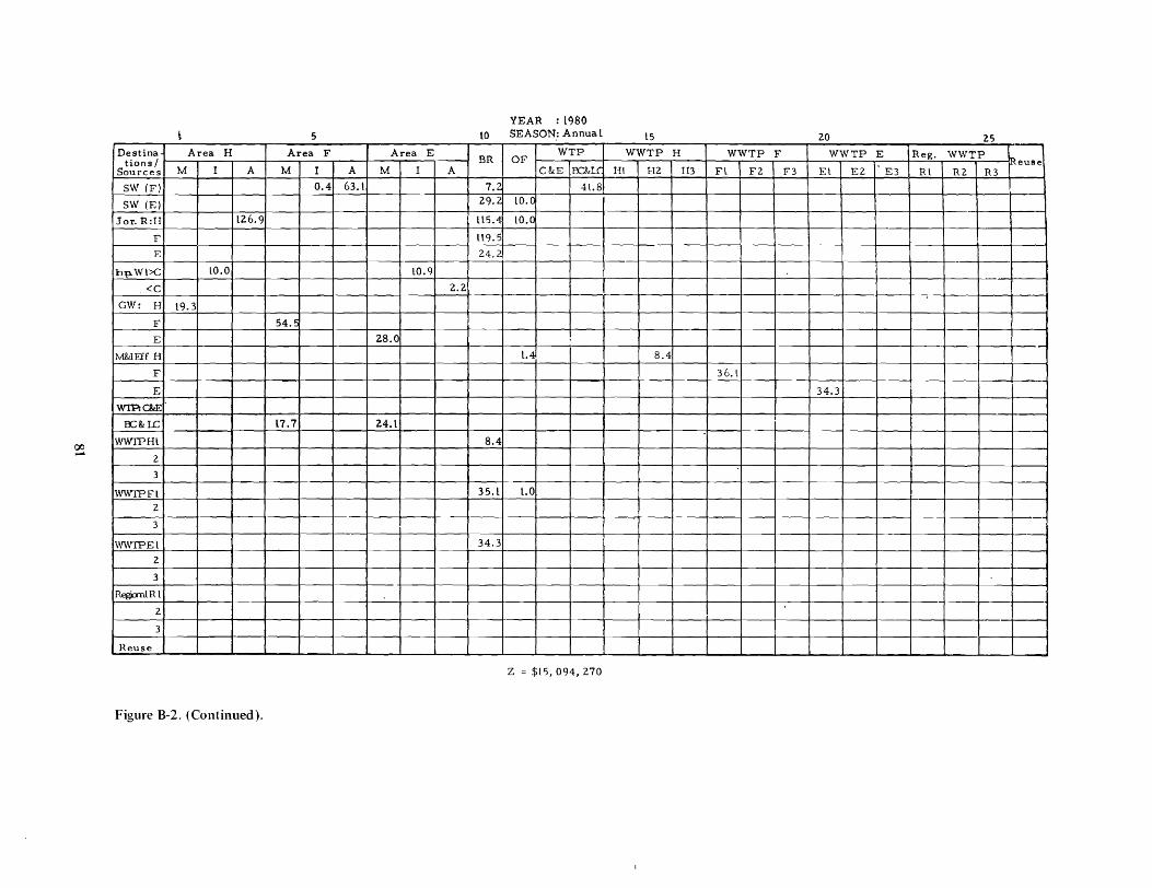
YEAR : L980 5 LO SEASON: Annual l5 20 25
Destina Area H Area F Area E WTP WWTP H WWTP F WWTP E Reg. WWTP tians I BR OF eU8e
Sources M I A M I A M I A C&:E EC.~ Hl H2 H3 Fl F2 F3 El E2 E3 Rl R2 R3
SW (F) 0.4 63.1 7.2 4l.8
SW (E) 29.L LO.C
Jar. R:H L26.9 ll5.4 lO.O
F ll9.5
E 24.£ -
hp.Wl>C W.O lO.9
<C 2.2
GW: H L9.3
F 54. ~
E 28.0 -M&IFif H L.4 8.4
F 36.l
E 34.3
WfP:c&E
OC&tLC l7.7 24.L
~ WWfPHl 8.4 - 2
3
WWTPFl 35.L l.0
2 -3
WWTPEl 34.3
2
3
Regi:mlRl
2
3
Reuse
Z = $L5, 094, 270
Figure B-2. (Continued).
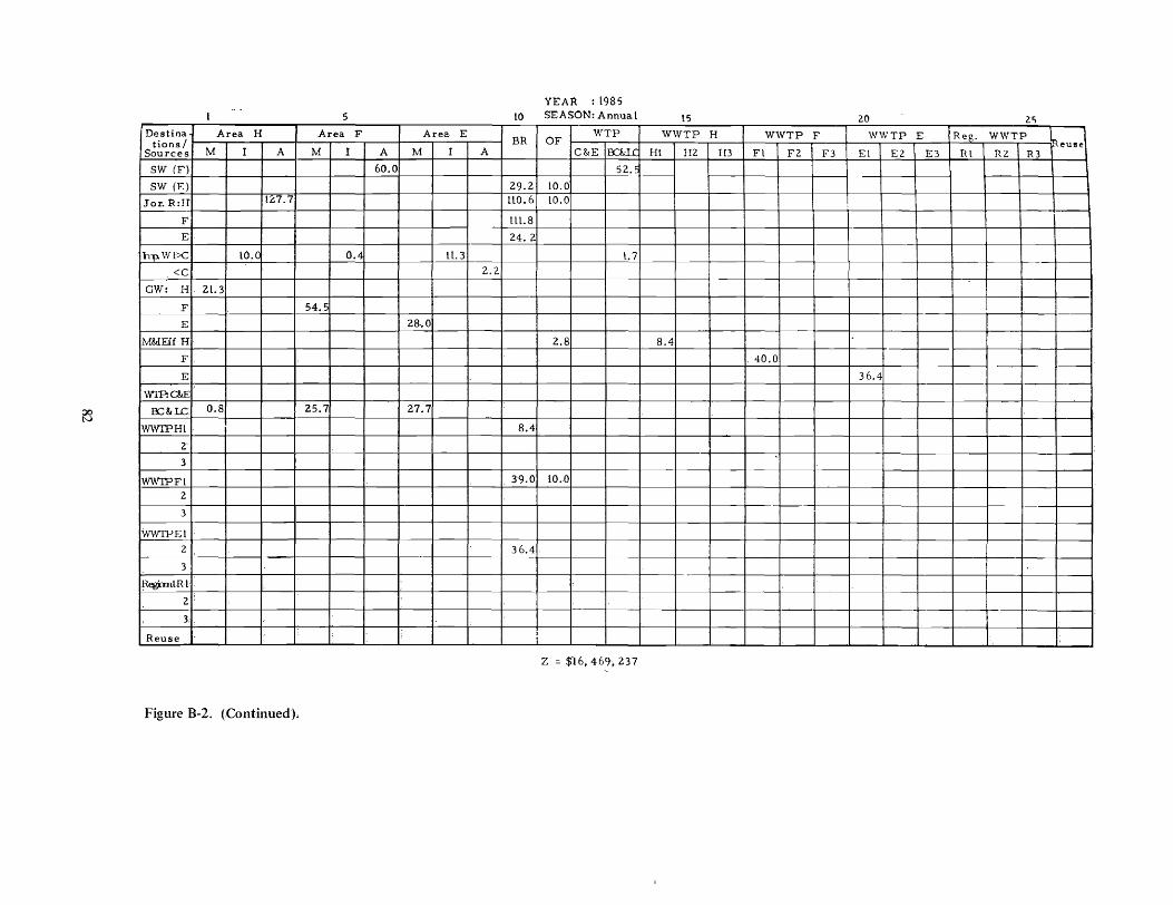
YEAR : t985
5 LO SEASON: Annual 15 20 l'l
Destina Area H Area F Area E OF
WTP WWTP H WWTP F WWTP E Reg. WV1TP tions / BR eUlSe
Sources M I A M I A M I A C&E 1K:&lC HI H2 H3 Fl F2 F3 El E2 E3 RI n,2 R3
SW (F) 60.0 52.t:;
SW (E) 29.2 LO.O
Jar. R:H L2.7.7 LtO.6 LO.O
F LLL.8
E· 24. 2
'hllo Wl>C LO.C O~ LL. 3 l.7
<c 2.2
GW: H.2L.3
F· 54.5
E 28.0
M&IEff H, 2.8 8.4
F. .40.0
E 36.4
WTP:c&E
?S OC&I.C 0.8 25.7 27.7
WWIPHI 8.4
2
3
WWIPFl 39.0 LO.O
2
3
WWTPEl
2 36.4 .
3
f{egimlRl'
2'
3; .
Reuse I
~
Z = $'16,469,237
Figure B-2. (Continued).
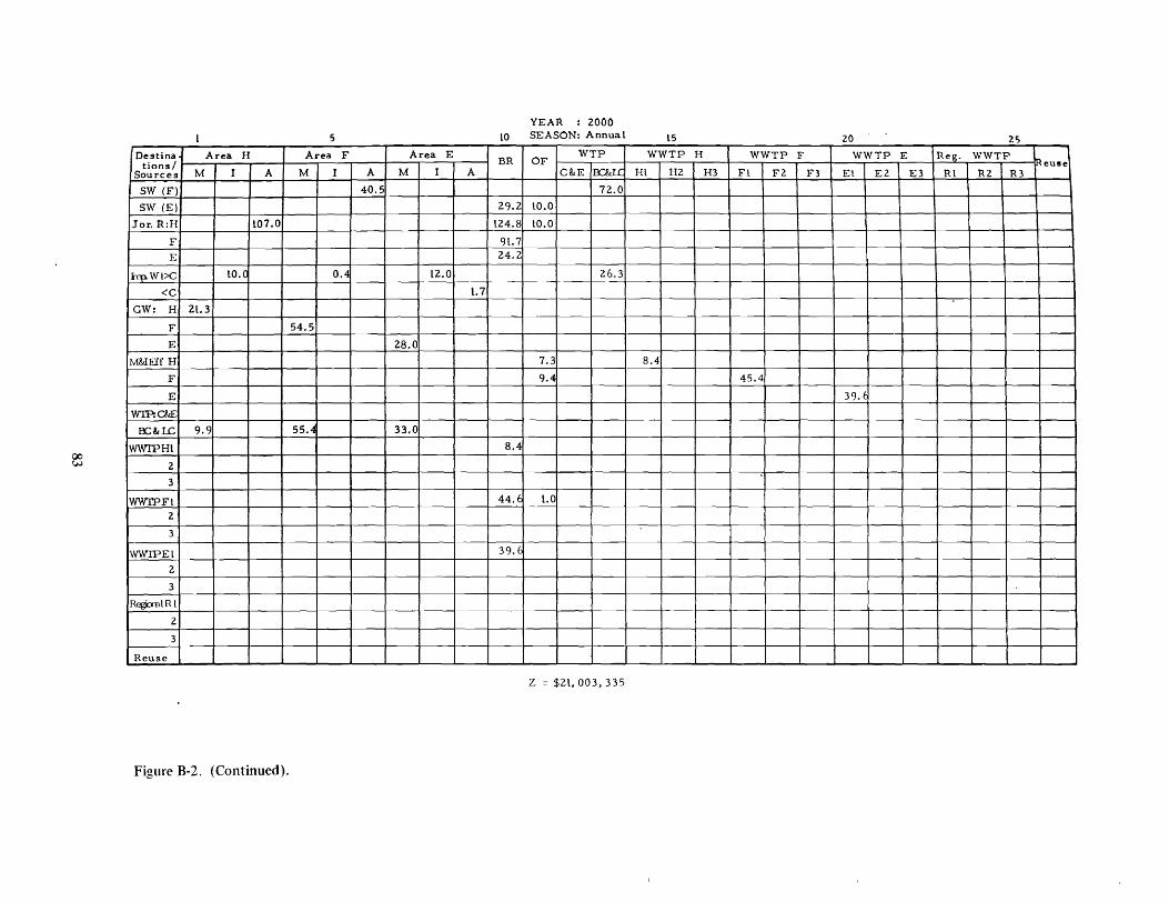
00 W
Destina Area H tions /
Sources M I A
SW (F)
SW (E)
Jor.R:H 107.0
F
E
irp. Wl>C 10.0
<C
GW: H 2l. 3
F
E
M&IElfH
F
E
WI'P:c&E
OC:&LC 9.9
WWfPHl
2
3
WWfPFl 2
3
WWIPEl
2
3
Regi:rnlRl
2
3
Reuse
Figure B-2. (Continued).
5
Area F Area E
M I A M I
40.5
0.4 12.0
54.5
28.0
55.4 33.0
YEAR : 2000 LO SEASON: Annua 1 l5 20 25
BR OF WTP WWTP H WWTP F WWTP E Reg. WWTP
eUlle A C&E oc:&LC Hl H2 H3 Fl F2 F3 El E2 E3 Rl R2 R3
72.0
29.2 10.0
124.8 to.O
9l.7 24.2
26.3
l.7
7.3 8.4
9.4 45.4
39. t
8.4
44.t LO
39.6
--'------
Z = $2l, 003, 335
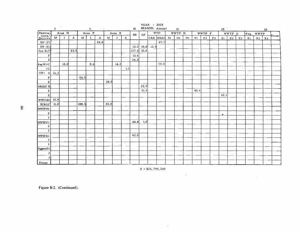
YEAR 2020
5 to SEASON: Annua L 2.5 L5 20 -
Destina Area H Area F Area E OF
WTP WWTP H WWTP F WWTP E Re~. WWTP tions / BR euse
Sources M I A M 1 A M I A C&E 1JX".&l{ HL HZ H3 FL FZ F3 El EZ E3 Rl R2 R3
SW (F) 24.8 87.7
SW (E) l6.3 lO.O l2.9
Jor. R:H 83.0 L37.3 LO.O
F 6l.4
E 24.2
iTpWl>C LO.O 0.4 l4.2 59.9 I
<C L.2
GW: H 2t3
F 54.5
E 28.(
M&IEff H 22.9
F 3L.6 45.4
E 42.5
WTP:c&E L2.9
OC&:LC U.8 LOO.3 35.5
~ WWfPHl
2 . 3
WWTPFl 44.4 L.O
2
3
WWIPEl 42.5
2
3
ReghntRl ~.
2.
3
Reuse .', --
Z = $26, 795, 240
Figure B-2. (Continued).
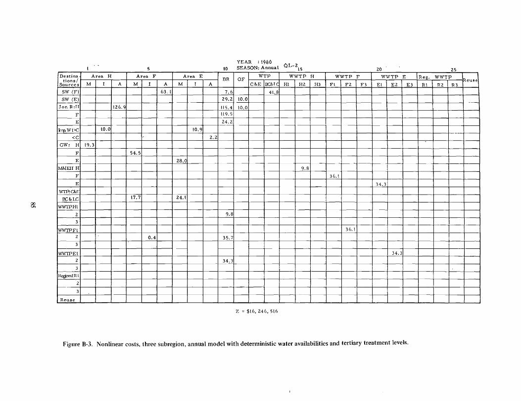
5
YEAR : 19fsO to SEASON: AnnuaL OL-2L5 25 20 --
Destina Area H Area F Area E OF
WTP WWTP H WWTP F WWTP E Reg. WWTP tions / BR It>euse
Sources M r A M I A M I A C&:E Er.-&:1.C Hl H2 H3 Fl F2 F3 El E2 E3 Rl R2 R3
SW (F) 63. L 7.6 4L.8
SW (E) 29.2 LO.O
Jor. R:H l26.9 LL5.4 LO.O
F Ll9.5 t--
E 24.2
h~Wl>C LO.O LO.9
<C / 2.2
GW: H 19.3
F 54.5
E 28~
M&IEff H 9.8
F 36. L
E 34.3
W1P:c&:E
OC&:LC l7.7 24.l
~ WWIPHl
2 9.8
3
WWIPFl 36.l
2 0.4 35.7
3
WW1PEl 34.3
2 34.3
3
HegrinlRl
2
3
Reuse
Z = $L6, 246, 516
Figure B-3. Nonlinear costs, three subregion, annual model with deterministic water availabilities and tertiary treatment levels.
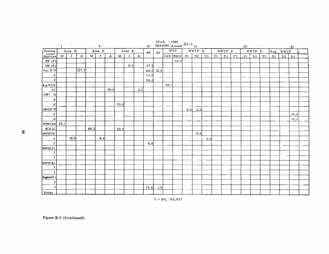
5 YEAR : 1985 OL-3 SEASON: AnnuaL 15 25 to 20
Destina Area H Area F Area E OF
WTP WWTP H WWTP F WWTP E Reg. WWTP tions/ BR euse
Sources M I A M I A M I A C&E oc&l.( HL H2 H3 FL F2 F3 EL E2 E3 Rl R2 R3
SW (F) Lt2.5
SW (E) LL. 3 27.9
Jor. R:H L27.7 LtO.6 to.O
F l LL. 8
E 24.2
hpWL>C 22. L
.<C 60.0 2.2
GW: H
F
E 23.4
M&IEff H 8.4 2.8 J F -:10.0 J E 36.4
WTP:c&E 22.L
~ OC&lC 80.2 32.3
WWTPHL 8.4
2 LO.O 0.4 0.8
3 0.8
WWfPFL 2
3
wwrPEl
2
3
RegimLRL
2
3 75.4 L.O
Reuse
Z = $21, 3L6,827
Figure 8-3. (Continued).
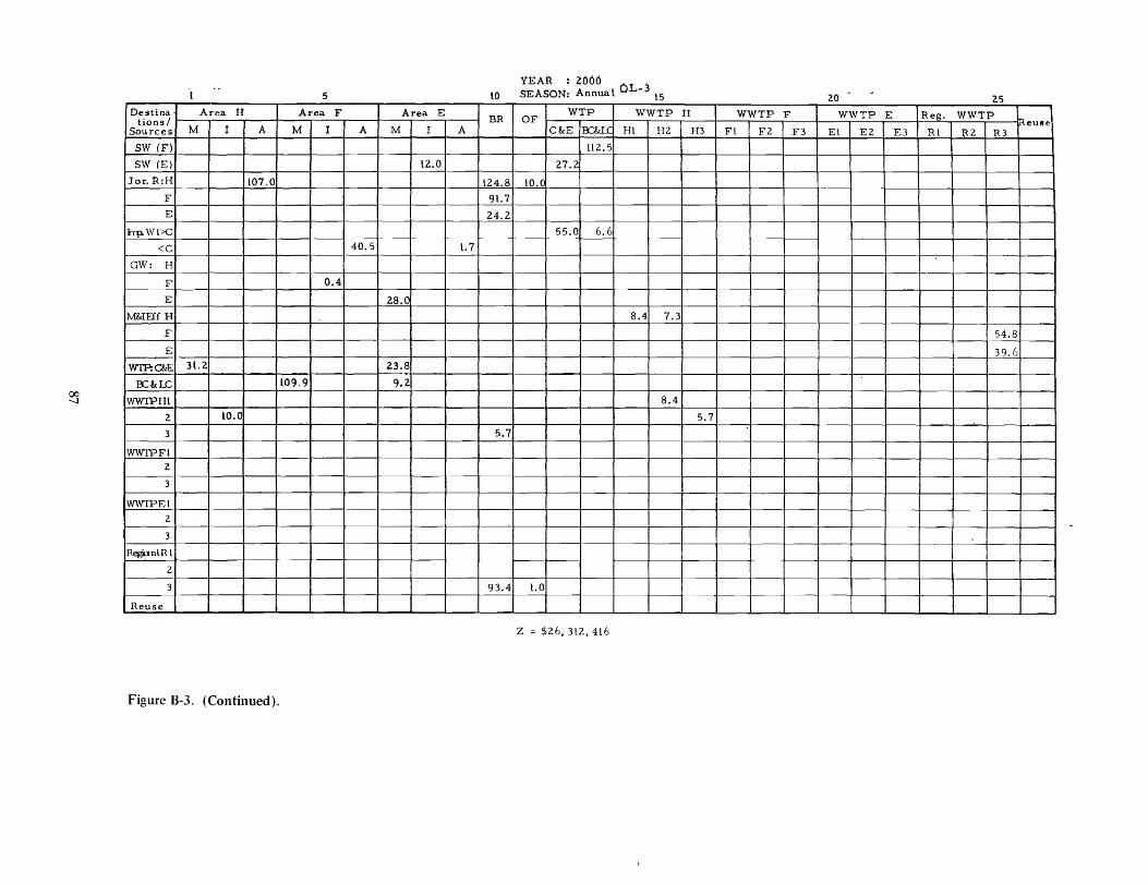
00 -..I
Destina Area H tians /
Sources M I A
SW (F)
SW (E)
Jor. R:H L07.0
F
E
hp.WI>C
<c GW: H
F
E
M&IBf H
F
E
wrP:c&E 3L2
OC&I.C
WWIPHL
2 lO.a 3
WWTPFI
2
3
WWfPEl
2
3
RegnnlI<l
2
3
Reuse
Figure B-3. (Continued).
5
Area F Area E
M I A M I A
L2.0
40.5 L.7
0.4
28.0
23.8
l09.9 9.2
LO
YEAR : 20M SEASON: Annual QL-3 l5
25 20 - ~ - ~
WTP WWTP H WWTP F WWTP E Reg. WWTP BR OF euse C&E 10C&lC Hl H2 H3 Fl F2 F3 El E2 E3 Rl R2 R3
LL2.5
27.2
L24.8 LO.C
9L.7
24.2
55.0 6.6
8.4 7.3
54.8
39.6
8.4
5.7
5.7
93.4 L.O
Z = $26, 3l2, 4L6

5 to YEAR : 2020 OL-3 SEASON: Annua L L5 25 20
Destina Area H Area F Area E WTP WWTP H WWTP F WWTP E Reg. WWTP tions I BR OF euse
Sources M I A M I A M 1 A C&E 10C&1.C Hl H2 H3 Fl F2 F3 El E2 E3 Rl R2 R3 SW (F) tt2.5
SW (E) L4.2 25.0
Jor. R:H 83.0 L37.3 LO.O
F 6L.4
E 24.2
irp. Wl>C 55.0 29.5 --<C 24.8 L.2
GW: H 2L.3
F LB.O 0.4
E 2Bi
M&IEff H 22.9
F 77.0
E 42.5
VITP:c&E 24.7 30.3
OC&lC l36.8 5.2 ~ WWfPHl
2 lO.O L2.9 3 L2.9
WWTPFl 2
3 ! WWTPEl
i
2
3
RegirBlRl
2
3 Ll8.5 L.O
Reuse ~
Z = $32, 553, L85
Figure B-3. (Continued).
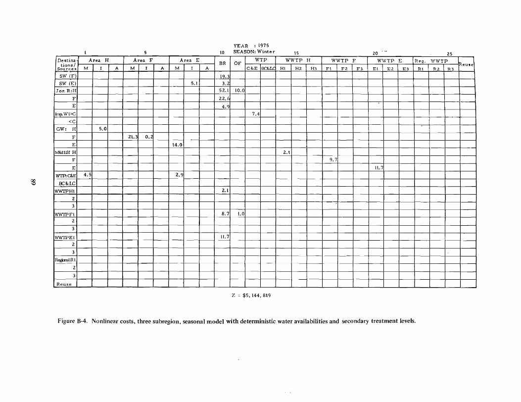
YEAR : 1975 5 to SEASON: Winter l5 20 25
Degtina Area H Area F Area E OF WTP WWTP H WWTP F WWTP E Re~. WWTP
tions/ BR euse Sources M I A M I A M I A C&E OC.&.U: HI H2 H3 Fl F2 F3 El E2 E3 Rl R2 R3
SW (F) t!l.3 SW (E) S.l 3.2
'--'
Jor. R:H S2.t lO.O
F 22.~
E 4.9
hl\Wl>C 7.4 -
<c GW: H 5,0
F 21.3 0.2
E l4.0
M&lEIfH 2.l
F 9.7
E tL. 7
WTP:c&E 4.5 2.9
~ OC&1C
wwrPHl 2.l
2
3
WW'IPFl S.7 l.O 2
3
WWTPEl lL. 7
2
3
Regk:mtRl
2
3
Reuse -- '---- - '---
Z = $5. L44. SL9
Figure B-4. Nonlinear costs, three subregion, seasonal model with deterministic water availabilities and secondary treatment levels.
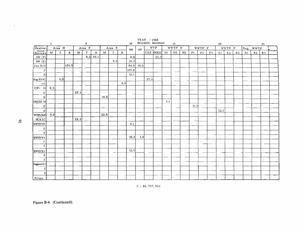
YEAR 1980 5 to SEASON: Summe r 15 20 21}
Destina Area H Area F Area E WTP WWTP H WWTP F WWTP E Reg. WWTP tions / BR OF ... eUlle
Sources M I A M I A M I A C&E 'oc.&L( HI H2 H3 Fl F2 F3 El E2 E3 Rl R2 R3
SW (F) 0.2 63. L 0.8 23.3 -- -- -SW (E) 5.5 21.2
Jor. R:H L26.9 89.8 LO.O
F l07.0
E L8.l I
hp.Wl>C 5.0 27.5 -<C 2.2
GW: H 8.5
F 27.3
E L4.0
MMEIf H 3.l
F L I. 5
E L2.5
WIP:c&E 5.0 22.5
tS OC&1C 23.3
WWTPHI 3.L
2
3
WV-lTPFI to.5 L.O
2
3
wwrPEl 12.5
2
3
ReginilRl
2
3
Reuse - -- - - - - - - '---- -----
Z = $H, 727, 522
Figure 8-4. (Continued).

\0 W
5
Destina Area H Area F tions/
Sources M I A M I
SW (F) O. LO
SW (E)
Jor. R:H
F
E
irp. Wl>C
<c GW: H 5.0
F 27.4 O.L
E
M&IE1fH
F
E
WTP:c&E 7.5 OC&LC
wwrPHL
2 3
WWfPFI 2
3
WWIPEl
2
3
ReghnlRI
2
3
Reuse
Figure B-4. (Continued).
Area E
A M I A
5.7
L4.0
4.9
YEAR : 19B5 10 SEASON: Winter 15 20 2.5
WTP WWTP H WWTP F WWTP E Reg. WWTP BR OF euse C&E K.&lC Ht H2 H3 FL F2 F3 El E2 E3 Rl R2 R3
L9.2 2.6
50.7 LO.O
20.0
4,<1 L2.4 _._- --
3.5
L2.3
l2!l
3.5
LO.O 2.3
L2.9
7, = $ (;, L3 7, (,58
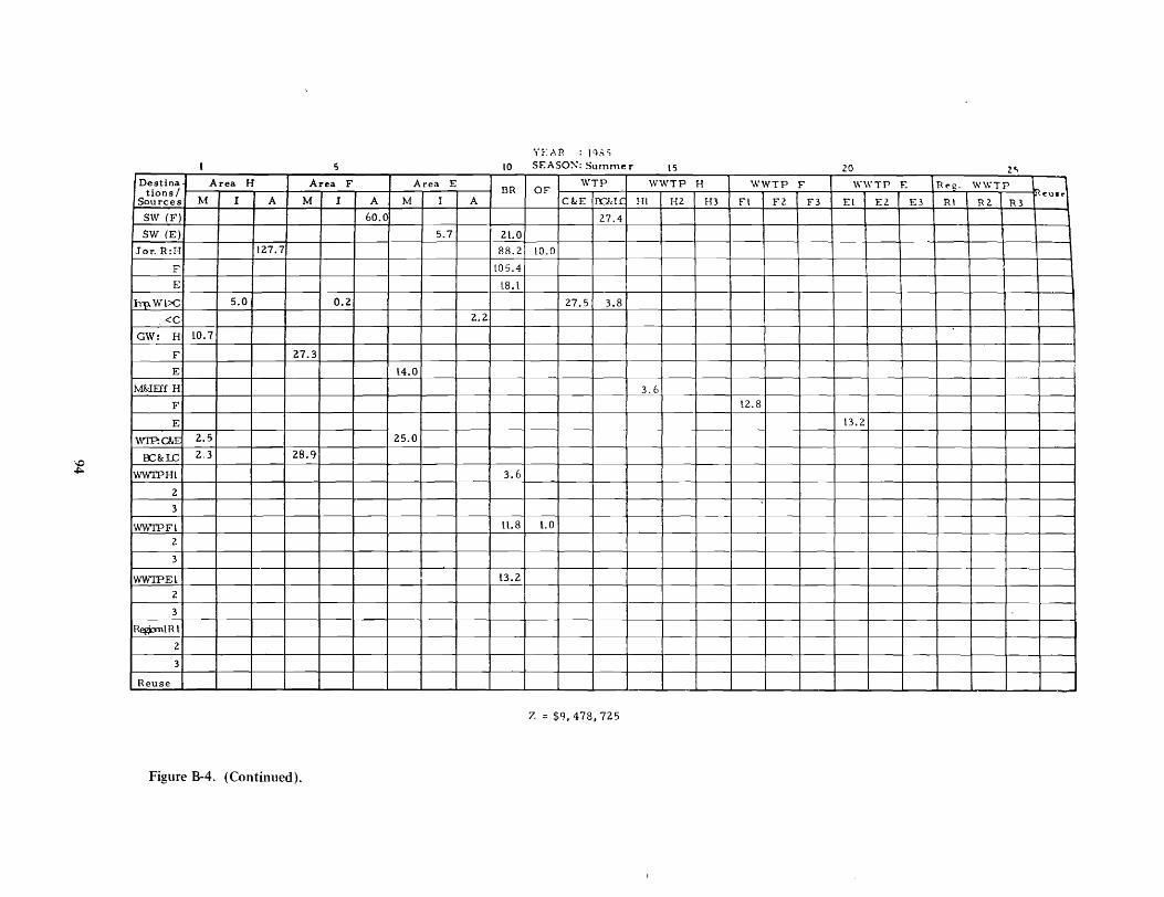
iTAP. : I():;';
5 10 SEASO~: Summer 15 20 zc, Destina Area H Area F Area E WTP WWTP H WWTP F WWTP F. R~R· W\I,:TP
tions / DR OF '~IJ'" Sources M I A M I A M I A C&E oc.&lL HI HZ H3 FI F2 F3 EI E2 E3 RI RZ R3
SW (F) 60.0 27.4
SW (E) 5.7 2l.0 Jor. R:H l27.7 88.2 lO.O
F l05.4
E l8.1
~Wl>C 5.0 0.2 27.5 3.8
<C 2.2
GW: H 10.7
F 27.3
E \4.0
M&IEff H 3.6 F 12.8
E \3.2
WI'P:c&E 2.5 25.0
~ OC&l.C 2.3 28.9
WWfPHl 3.6
2 3
WWT'PFl ll.8 l.0
2
3
WWIPEl \3.2
2
3
RegrrnlR I
2
3
Reuse
Z = $9,478,725
Figure 8-4. (Continued).
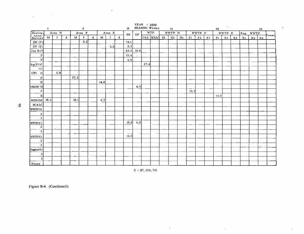
\0 VI
r Destina Area H tions /
Sources M I A
SW (F)
SW (E)
Jor. R:H
F
E
h-p. Wl>C
<C
GW: H 5.0
F
E
M&lEff H
F
E
WI'P:c&:E LO.6
OC&:J£
wwrPHL
2
3
WWfPFI 2
3
WWIPEI
2
3
ReghnIRl
2
3
Reuse
Figure B-4. (Continued).
5
Area F Area E
M I A M 1 A
0.2
6.0
27.2
L4.0
LO. L 6.7
YEAR : 2000 to SEASON: Winter l5 20 25
WTP WWTP H WWTP F WWTP E Reg. WWTP BR OF eUl!le C&:E 10ClM Hl H2 H3 FL F2 F3 El E2 E3 RL RZ R3
19.1
2.3
49.3 to.O
L5.4
6.9
27.4 --1"---'
J
I
---I 4.9
L6.9
L4.0
10.0 6.9
L4.0
Z = $7,652, 72L

\J,.? 0'1
5
Destina Area H Area F tions /
Sources M I A M I
SW (F)
SW (E)
Jor. R:H l07.0
F
E
lirpWl>C 5.0 0.2
<C
GW: H lO.7
F 27.3
E
M&IFIf H
F
E
WTP:c&E
OC&lC U.2 49.8
WWI'PHl
2
3
W'WTPFl 2
3
WWTPEl
2
3
RegbnLRl
2
3
Reuse
Figure B-4. (Continued).
Area E
A M I A
40.5
6.0
L.7
l4.0
27.5
1.2
YEAR : 20M to SEASON: Summer L5 20 2S
OF WTP WWTP H WWTP F WWTP E Reg. WWTP BR euee
C&E 10C.&l.( Hl H2 H3 Ft F2 F3 El E2 E3 Rl R2 R3
46.9
20.7
L03.L lO.O
9l. 6
l8.l "J
27.5 l5.3 --r-
0.8 4.2
l7.5
l4.3
4.2
r-
L6.5 l.0
l4.3
I
! Z = $ll, 634, 685
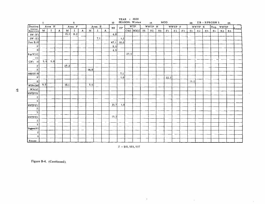
\0 -....)
5
Destina Area H Area F tions/
Sources M I A M I
SW (F) l5.l 0.2
SW (E)
Jor. R:H
F
E
~Wl>C
<C
GW: H 5. t 5.0
F 27.2
E
MMEIf H
F
E
wrP:c&E 9.9 lO.l
OC&l.C
WWIPHL
2
3
WWfPFl Z
3
WWTPEl
Z
3
RegDnlRl
2
3
Reuse
Figure B-4. (Continued).
Area E
A M I A
7.l
l4.0
7.5
YEAR 2020 to SEASON: Winter l5 MOD 20 - ZB == RPROBW 5 2S
BR OF WTP WWTP H WWTP F WWTP E ReJi. WWTP
~eulle C&E loc.&LC Hl HZ H3 Fl F2 F3 El E2 E3 Rl R2 R3
4.0
l.Z
47.l lO.O
8.6 4.9
27.5
7.l
l.0 22.7
lS.2
2l.7 l.O
lS.2
Z == $lO, 503,537
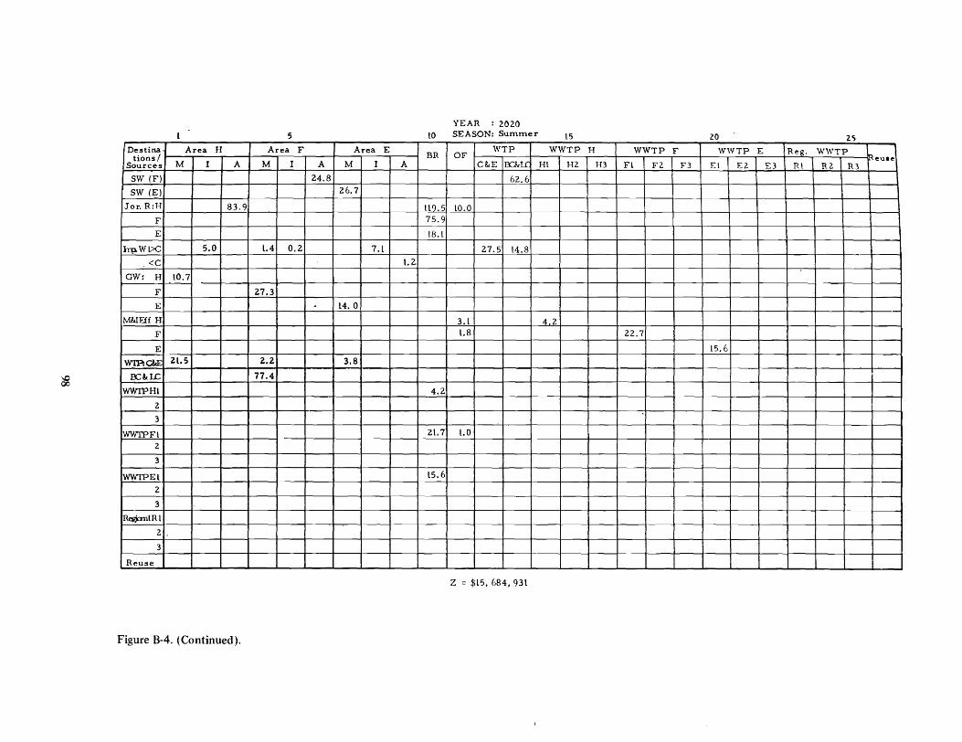
YEAR : 2020
5 to SEASON: Summer l5 lO lC; Destina Area H Area F Area E
OF WTP WWTP H WWTP F WWTP E Re~. WWTP
tions I BR euae Sources M I A M I A M I A C&E Ioc&l.( Hl H2 H3 Fl F2 F3 El E2 E3 Rl R2 R3
SW (F) 24.8 62.6
SW (.E:) 26.7
Jor. R:H 83.9 l~.5 lO.O F 75.9
E l8.L
h1l- Wl>C 5.0 l.4 0.2 7.l 27.5 l4.8
<C l.2
GW: H lO.7
F 27.3
E . L4.0
M&IEIf H 3.t 4 2 F l.8 22.7
E l5.6
W1'P:c&E 2l.5 2.2 3.8
?i1 OC&LC 77.4
WWfPHl 4.2
2
3
'WWTPFl 21.7 l.O
2
3
WWIPEl LS.6
2
3
ReghnlRl
2 .
3
Reuse
Z = $L5, 684, 93l
Figure B-4. (Continued).
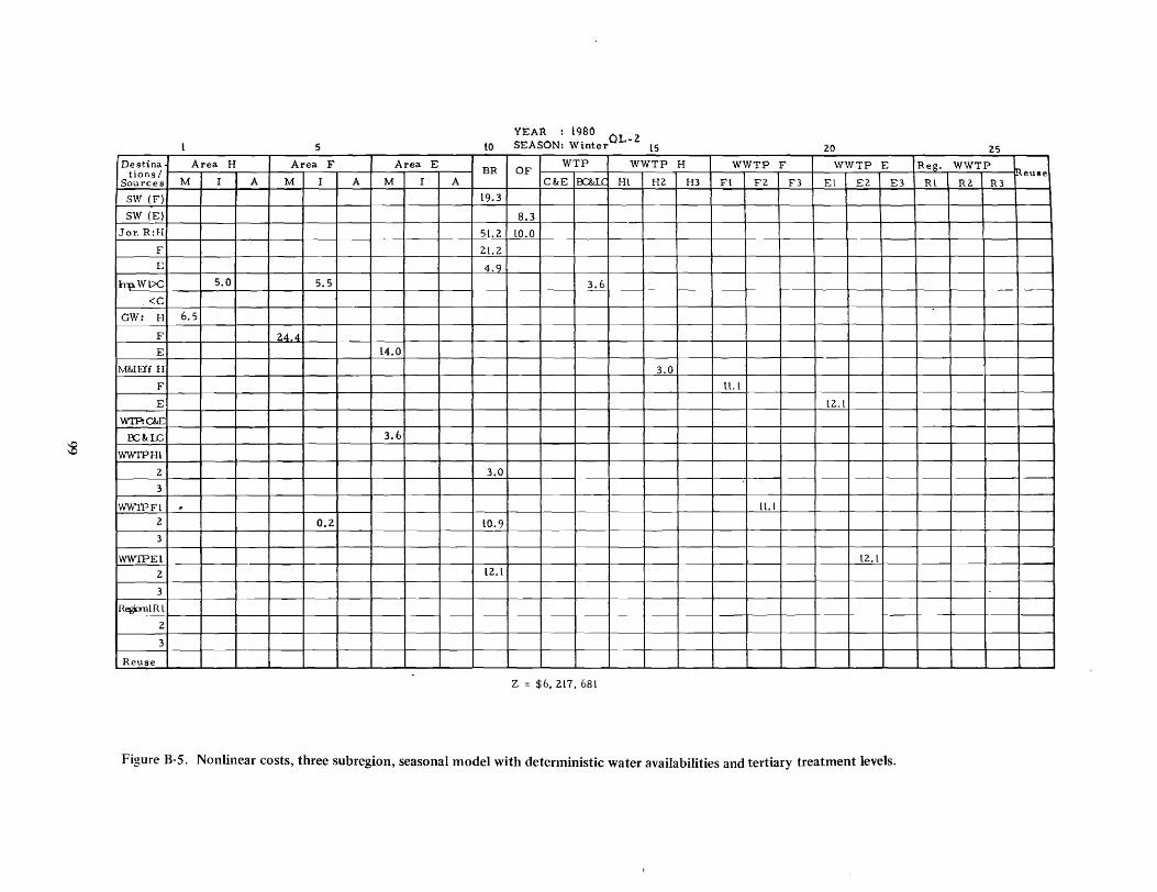
5 lO YEAR : 1980 OL-2 SEASON: Winter l5 25 20
Destina Area H Area F Area E OF
WTP WWTP H WWTP F WWTP E Reg. WWTP tions / BR eUlle
Sources M I A M I A M I A C&E loc.&LC Hl H2 H3 Fl F2 F3 El E2 E3 Rl R2 R3
sw (Fl 19.3
SW (El 8.3 Jor. R:H SL.2 lO.O
F 2l.2
E 4.!l hV-Wl>C 5.0 5.5 3.6
<C
GW: I-I 6.5
F 24.4 E t4.0
M&IEIf II 3.0
F tl.l
E l2. L
WTP:C&E
~ OC&r.c 3.6
WWTPHl
2 3.0 3
WV.,rTPFL " LL.l
2 0.2 LO.9 3
WWfPEl L2.t
2 L2.t
3
Regi:rnLR L
2
3
Reuse
Z = $6, 2t7, 68t
Figure 8-5. Nonlinear costs, three subregion, seasonal model with deterministic water availabilities and tertiary treatment levels.

5 'lEAR : 19AO OL-2
10 SEASO~: Summer lS zr, 20
Destina Area H Area F Area E OF
WTP WWTP H WWTP F WWTP E Reg. WWTP I ~u,J tions / BR Sources M r A M r A M I A C&E OC&LC Hl HZ H3 Fl F2 F3 El E2 E3 Rl RZ R3
SW (F) 63.l 24.3
SW (E) l6.7 lO.O
Jor. R:H L26.9 89.8 LO.O
F L07.0
E l8l.0
hp.WL>C 4.2 5.5 24.3 t--<C 2.2
GW: H LO.7
F 27.3
E L4.0
M&IEIfH 3. L
F LL.5
E L2.5
WIP:c&E
§ OC&:lC 2.8 23.3 22.5
WWfPHl
2 0.8 2.3
3
WWTPFl LL.5
2 0.2 LL.3
3
WWIPEL L2.5
2 L2.5
3
ReghnLRL
2
3
Reuse
z =: $9,325, 579
Figure B-5. (Continued).

5 YEAR : t985 QL-3
to SEASON: Winter l5 25 20
Destina Area H Area F Area E BR OF
WTP WWTP H WWTP F WWTP E Reg. WWTP tions / euse
Sources M I A M I A M I A C&E oc.&IL HL H2 H3 FL F2 F3 El E2 E3 Rl R2 R3
SW (F) O.L L9.2
SW (E) 5.7 2.6
Jor. R:H 50.7 LO.O
F 20.0
E 4.9
Ihp.Wl>C L2.4
<c GW: H L.5
F 27.L O.L
E L4.0
M&:IEIf H 3.5
F t2.3
E t2.9
WIP:c&E 7.5 4.9
§ OC&lC
WWfPHl 3.5
2 3.5
3
VVWTPFI 2
3
wwrPEl
2
3
ReghnlRl
2
3 24.2 L.O
Reuse - "--------
Z =: $8,492,097
Figure B-S. (Continued).

5 LO YEAR : L985 QL-3 SEASON: Summer l5 2.S 20
Destina Area H Area F Area E WTP WWTP H WWTP F WWTP E Reg. WWTP 1 tions / BR OF eU8e
Sources M I A M I A M I A C&E OC&LC Hl HZ H3 Fl F2 F3 El E2 E3 Rl R2 R3
SW (F) 9.0 l.0 77.4 SW (E) 5.7 2l.0
Jor. R:H l27.7 88.2 LO.O
F LQ5.4
E l8.l
hlJo Wl>C L5.5 f------t--
<c 60.0 2.2
GW: H L.4
F 3.8 0.2 -E t4.0 J M&IEff H 3.6
F l2.8 I
E l3.2 I wrP:C&E l5.5
§ 0::&1£ 52 4 25 0
wwrPHl 3 6
2
3 3.6
wwrPFl 2
3
WWrPEl
2
3
RegbnlRl
2
3 25.0 L.O
Reuse
Z = $LL, 580, 33t
Figure B-5. (Continued).

...... o w
Destina Area H tions /
Sources M I A
SW (F)
SW (E)
Jor. R:H
F
E
hp.WL>C
<C
GW: H I O.L
F
E
M&IFif H
F
E
WTP:C&E lO.6
OC&LC
WWIPHl
Z 4.9
3
WWfPFL 2
3
WWI'PEL
2
3
RegrrnlRL
2
3
Reuse
Figure B-S. (Continued).
5
Area F Area E
M I A M I
0.2
6.0
27.2
l4.0
LO.l 6.7
to
BR A
L9.L
2.3
49.3
l5.4
4.9
29.9
YEAR : 2000 SEASON: Winter CL-3 L5
OF WTP WWTP H
C&E ioc.&lC HL HZ
lO.O
27.4
4.2 0.7
4.2
L.O
Z = $10, 234,009
20 25 WWTP F WWTP E Reg. WWTP
eU!le H3 Fl FZ F3 El E2 E3 RL RZ R3
t----
L6.9
l4.0
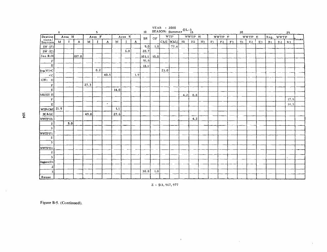
5 to YEAR 2000 OL-3 SEASON: Summer LS 20 25
Destina Area H Area F Area E BR
WTP WWTP H WWTP F WWTP E Reg. WWTP tions / OF euse
Sources M I A M I A M I A C&tE IOCM.C HL HZ H3 Fl FZ F3 El E2 E3 Rl R2 R3
SW (F) 9.0 LO 77.4
SW (E) 6.0 20.7
Jor. R:H L07.0 L03.l LO.O
F 9l. 6
E L8.L
h'pWl>C 0.2 23.0 . <c 40.5 l.9 i
GW: H j
F 27.3 I I
E l4.0
MMEIfH 4.2 0.8
F L7.5
E . L4.3
WI'P:c&E 2l.9 lol
~ OC&LC 49.S 27.6
WWIPHL 4.2
2 5.0 3
rwwwFL 2
3
WWTPEL
2
3
Regi:rnlR l
2
3 30.8 l.O
I Reuse - - -
Z = $l3. 967.977
Figure B-S. (Continued).
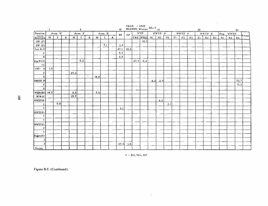
5 YEAR : 2020 OL-3 SEASON: Winter l5 21) to zo
Destina Area H Area F Area E OF
WTP WWTP H WWTP F WWTP E Reg. WWTP 1 tions I BR eUle
Sources M I A M I A M I A C&E oc.&l( Ht H2 H3 FL F2 F3 Et E2 E3 Rl RZ R3
SW (F) L9.3
SW (E) 7.l L.2
Jor. R:H 47.L LO.O
F 8.6 E 4.9
I~WL>C 0.2 27.5 0.4
<c GW: H L.O
F 27.2
E l4.0
M.&IFff H 4.2 2.9 23.7
F LS.2
E
WI'P:c&E l4.5 5.5 7.5
o OC&lC 19.7 Vl WWIPHL 4.2
2 5.0 2.l
3 2.L
YVWrPFl 2
3
WWIPEl
2
3
RegrinlRl
2
3 37.9 l.0
Reuse
Z = $12, 94IJ, 387
Figure B-5. (Continued).

5 10 YEAR 2020 QL-3 SEASON: Summer 15 25 20
Destina Area H Area F Area E WTP WWTP H WWTP F WWTP E Reg. WWTP ,
tions / BR OF .... euee Sources M I A M I A M I A C&E 10CkLC HI H2 H3 Ft F2 F3 El £2 E3 Rl R2 R3
SW (F) 28.1 59.3
SW IE) 7.L L9.6
Jor. R:H 83.9 LL9.5 10.0
F 75.9
E 18.L
irp. WI>C 0.2 27.5 L8.1
<C 24.8 1.2
GW: H to.7
F 27.3
E l4.0
tvf&lEIf H 4.2 3.1
F 24.5
E 15.6
WTP:c&.£ 21. 5 £'.0
~ OC&:u::: 52.9 24.5
WWTPHL 4.2
2 4.2
3 0.8 2.3
WWTPFI 2
3
WWIPEI
2
3
RegnnlRL
2
3 39.l 1.0
Reuse .- - -- --
Z = $L8, 958, 717
Figure B-5. (Continued).

5 YEAR t975 L-L SEASON: AnnuaL t5 25
Stochastic LO 20
Destina Area H Area F Area E OF
WTP WWTP H WWTP F WWTP E Reg_. WWTP eU8~1 tions/ BR Sources M I A M I A M I A C&E ioc..&l( Hl H2 H3 Fl F2 F3 El E2 E3 RL R2 R3
SW (F) L4.6 25.8 I
SW (E) 2l.0
Jor. R:H 132.6 ll4.2 LO.O
F l27.4
E 24.2
irp. Wl>C LO.O 0.4 to.2 4.8
<C 56.7 2.9
GW: H 13.3
F 54.5
E 28.0 ----M&IE1f H 6.8
F 3l.4
E 33.0
WTP:c&E
§ OC&LC 8.6 22.0
wwrPHl 6.8
2
3
WW'IPFl 30.4 1.0
2
3
WWTPEl 33.0
2
3
RegOnlRL
2
3
Reuse - ~ - I
Z = $13, 574,050
Figure B-6. Nonlinear costs, three subregion,annual model with stochastic water availabilities and secondary treatment levels.
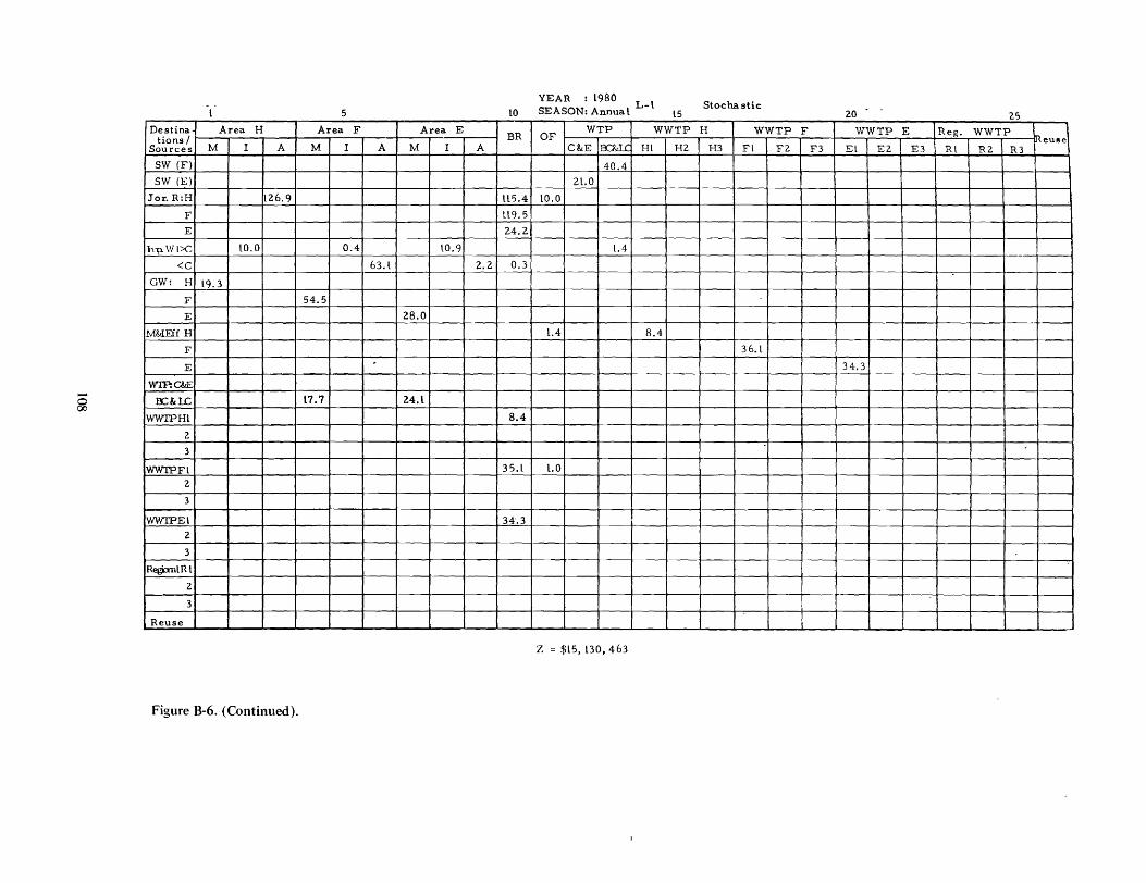
5 YEAR : 19S0 L-L
to SEASON: Annua L LS 2.5 Stochastic
20
Destina Area H Area F Area E BR OF
WTP WWTP H WWTP F WWTP E Reg. WWTP tions / eU8e
Sources M I A M I A M I A C&'E iOCM.C Hl H2 H3 Fl F2 F3 El E2 E3 Rl R2 R3
SW (F) 40.4
SW (E) 2t.0
Jor.R:H l26.9 U5.4 lO.O F tt9.5
E 24.2
h--p.Wl>C LO.O 0.4 lO.9 L.4
<c 63.t 2.2 0.3
GW: H L9.3
F 54.5
E 28.0
M&IEifH L.4 8.4
F 36. L
E 34.3
W'IP:c&E
~ OC8.:1C l7.7 24.l
WWIPHl 8.4
2
3
WWTPFl 35.l l.0
2
3
wwrPEl 34'.3
2
3
ReghnlRl
2
3
Reuse
Z = $l5, no, 463
Figure B-6. (Continued).

5 YEAR : 1985 L-L
10 SEASON: Annua L tS 2.S Stochastic
20
Destina Area H Area F Area E OF
WTP WWTP H WWTP F WWTP E Reg. WWTP tions/ BR In euse
Sources M I A M I A M I A C&E IOCM.C Hl H2 H3 Fl F:2 F3 EI E2 E3 Itl R2 R3
SW (F) 40.4
SW (E) 2L.0
Jor. R:H 127.7 110.6 LO.O
F 1Il.8
E 24.2
IhpWL>C 10.0 0.4 IL. 3 13.8
.<C 60.0 2.2 1.0
GW: H 21.3
F 54.5
E 28.0
M&lEff H 2.8 8.4
F 40.0
E 36.4
WIP.c&tE
OC&u:; 0.8 25.7 27.7
~ wwrPHL 8.4
2
3
Iw\VTPFI 39.0 1.0
2
3
WWIPEl 36.4
2
3
Heghulnl
2.
3
Reuse
z = $16,539,771
Figure B-6. (Continued).

5 to YEAR : 2000 L-l SEASON:Annual 25
Stochastic l5 2.0
Destina Area H Area F Area E BR OF
WTP WWTP H WWTP F WWTP E Reg. WWTP tiC''1S / eUlle
~~.:es M I A M I A M I A C&E iK.&tC Hl H2 H3 Ft F2. F3 El E2 E3 Ri R2 R3
SW (F) 0.4 4.2 35.8
SW (E) 2[.0
Jar. R:H L07.0 l24.8 lO.O
F 9L.L E 24.2
h~WL>C to.O L2.0 62.5 r--
<C 40.5 L.7 L.O
GW: H 2l.3
F 54.5
E 28.0
M&IEIf H 7.3 8.4
F 9.4 45.4
E 39.6
WI'P:c&E
o OC&LC 9.9 55.4 33.0
WWfPHt 8.4
2
3
WWTPFl 44.4 l.0
2
3
WWTPEl 39.6
2.
3
RegbnLRl
2
3
Reuse ~ - ~ "--- -- ~- - - - - --
Z = $2\,057, 2_5l
Figure B-6. (Continued).
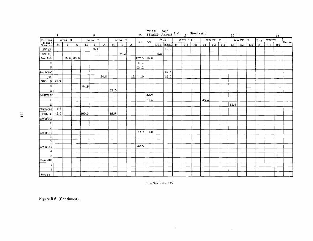
..... .....
Destina Area H tions/
Sources M I A
SW (F)
SW (E)
Jor. R:H 10.0 83.0
F
E
Ihp.WI>C
<C
GW: H 2l.3
F
E
M&IFif H
F
E
WTP:c&E 6.8
OC&LC 17.9
WWfPHl
2.
3
WWTPFI 2.
3
WWTPEI
2
3
R~IRI
2
3
Reuse
Figure B-6. (Continued).
5
Area F Area E
M I A M I A
0.4
l4.2
24.8 L.2
54.5 28.0
100.3 35.5
10
BR
127.3
6L.4
24.2
L.O
44.4
42.5
YEAR : 2.02.0 SEASON: Annual L-L l5
Stochastic
OF WTP WWTP H WWTP F
C&E EC&U: Hl H2 H3 Fl F2
40.0
6.8
10.0
84.5
29.0
22.9
31.6 45.4
l.0
z = $27,648,835
20 25
WWTP E Reg. WWTP neUl!le
F3 El E2 E3 Rl R2 R3
42.5
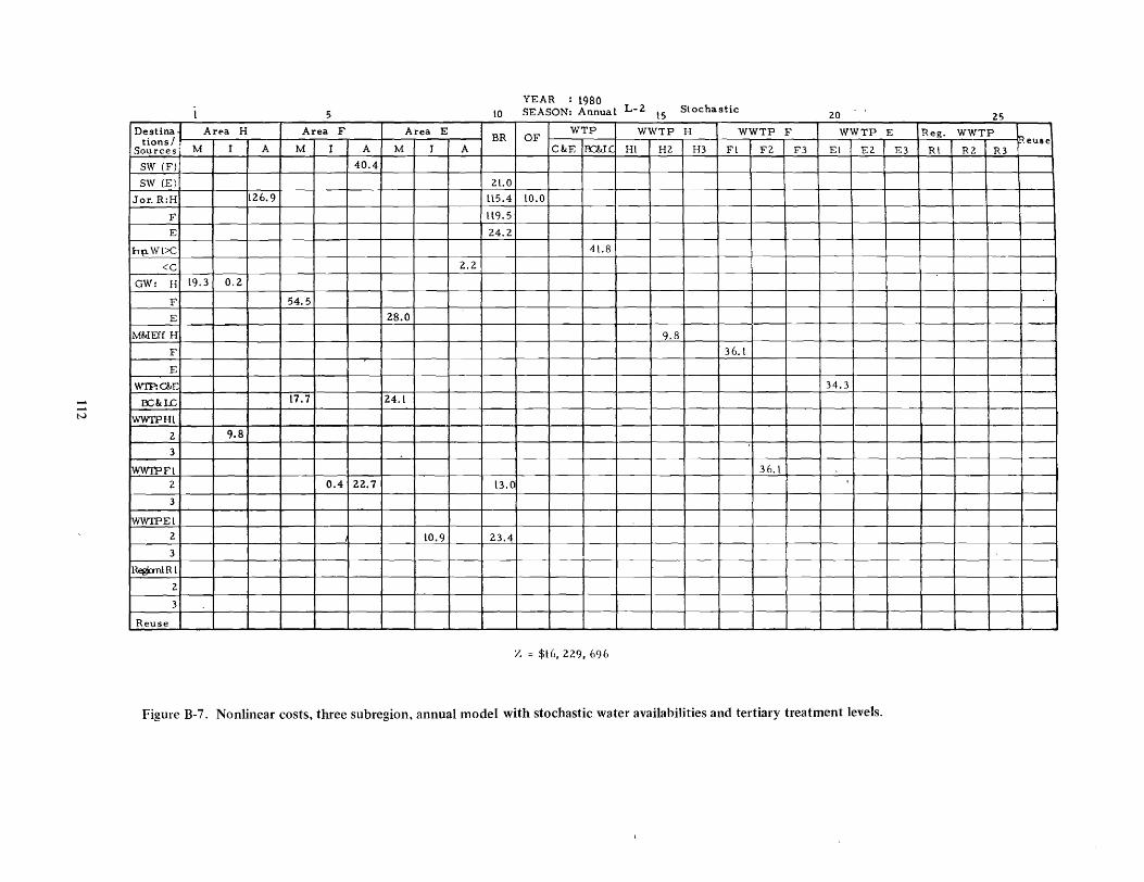
5
YEAR : L9BO to SEASON: AnnuaL L-2 l5 Stochastic 25 20
Destin~4 Area H Area F Area E OF
WTP WWTP H WWTP F WWTP E Reg. WWTP tions/ , BR .euse
Sources' M I A M I A M I A C&E OC:&l( HL H2 H3 Fl F2 F3 El E2 E3 RL R2 R3
SW (F) 40.4
SW (E) 2l.0
Jor. R:H t26.9 U5.4 to.O
F ll9.5
E 24.2
h-p. WL>C 41.8
<C 2.2
GW: H t9.3 0.2
F 54.5
E 28.0
M&IEffH 9.8
F 36. L
E
wrP.c&E 34.3 --OC&u:; L7.7 24.l
...... N WWTPHl
2 9.8
3
IW\V'IPFl 36. L
2 0.4 22.7 L3.0
3
WynpEL
2 LO.9 23.4
3
HegiTnLRI
2
3
Reuse
Z = $ttJ, 229, 696
Figure B-7. Nonlinear costs, three subregion, annual model with stochastic water availabilities and tertiary treatment levels.
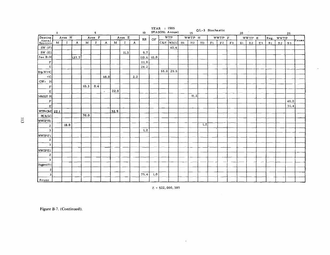
5
YEAR L985 to SEASON: AnnuaL
QL-3 Stochastic t5 20 25
Destina Area H Area F Area E WTP WWTP H WWTP F WWTP E Re~. WWTP tions / BR OF '0 eUlle
Sources M I A M I A M I A C&:E .oc.&:LC Ht H2 H3 Ft F2 F3 El E2 E3 Rl R2 R3
SW (F) 40.4
SW (E) LL.3 9.7
Jor. R:H t27.7 ltO.6 to.O
F lll.8
E 24.2
irp. Wl>C 55.0 29.5
<C 60.0 2.2
GW: H
F to.3 0.4
E 22.8
M&:IFff H It. 2
F 40.0 ~
E 36.4
WTP:c&E 22.L 32.9
OC&:LC 70.0
w wwrPHL
2 LO,O t.2
3 L.2
WW'IPFl 2
3
WWIPEl
2
3 I
HegbnlRl
2
3 75.4 l.0
Reuse
Z = $22,000, 385
Figure B-7. (Continued).
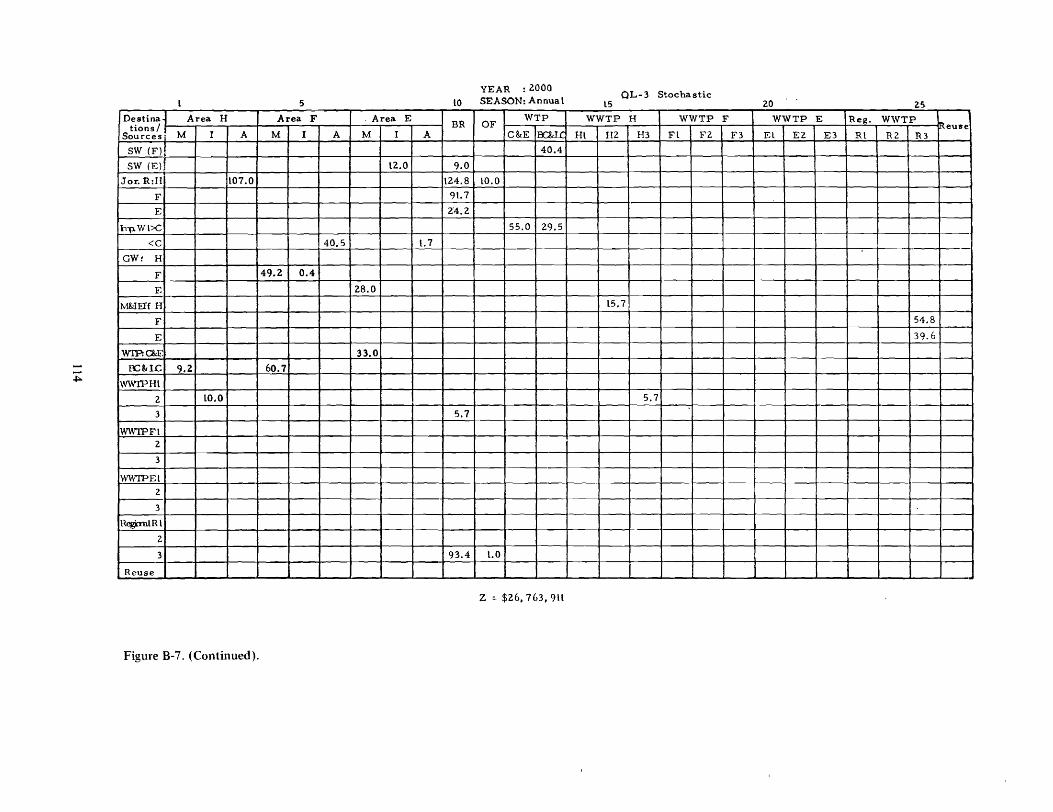
5
YEAR : 2000 LO SEASON: Annua l Z5
QL-3 Stochastic 20 l5
Destina ~ A rea H Area F . Area E BR OF
WTP WWTP H WWTP F WWTP E Reg. WWTP "'euse tions/!
Sources' M I A M I A M I A C&:E Ioc.&l( Hl H2 H3 Fl F2 F3 El E2 E3 Rl R2 R3
SW (F) 40.4
SW (E) l2.0 9.0
Jar. R:H l07.0 l24.8 lO.O
F 9l.7
E 2"4.2
h-p. Wl>C 55.0 29.5
<c 40.5 1.7 GW: H --
F 49.2 0.4
E 28.0
t-.1&IEff H l5.7
F 51.8 1
E 39.6 I
WIP.c&E 33.0 -- OC&:LC 9.2 60.7 +:0. WWIPHl
2 LO.O 5.7
3 5.7
WWTPFl 2
3
WWIPEl
2
3·
HegOnlRl
Z
3 93.4 l.0
Reuse
Z = $26.763, 91l
Figure 8-7. (Continued).
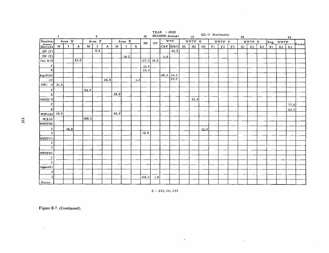
YEAR : 2020
5 10 SEASON: Annua I 25 QL-3 Stochastic
l5 20
Destina Area H Area F Area E OF
WTP WWTP H WWTP F WWTP E Reg. WWTP tions / BR "euse
Sources M I A M r A M I A C&E !ff'klC HI HZ H3 Fl FZ F3 EI E2 E3 Rl R2 R3 SW (F) 0.4 40.0
SW (E) 14.2 6 8 Jor.R:H 83.0 l37.3 10.0
F 6l.4 E 24.2
l~WI>C 48.2 36.3
<c 24.8 1.2 29.2
GW: H 2l.3
F 54.5
E 28.0
M&IEff H 22.9
F 77.0
E 42.5
WTP:Q.E 19.5 35.5
- :OC&l.C 100.3 VI
WWfPHl
2 10.0 12.9 3 12.9
IwwrPFI 2
3
WWIPEI 2
3
HegbnLnI
2
3 lt8.5 1.0
Reuse -
Z = $33, ()Ll, 693
Figure B-7. (Continued).

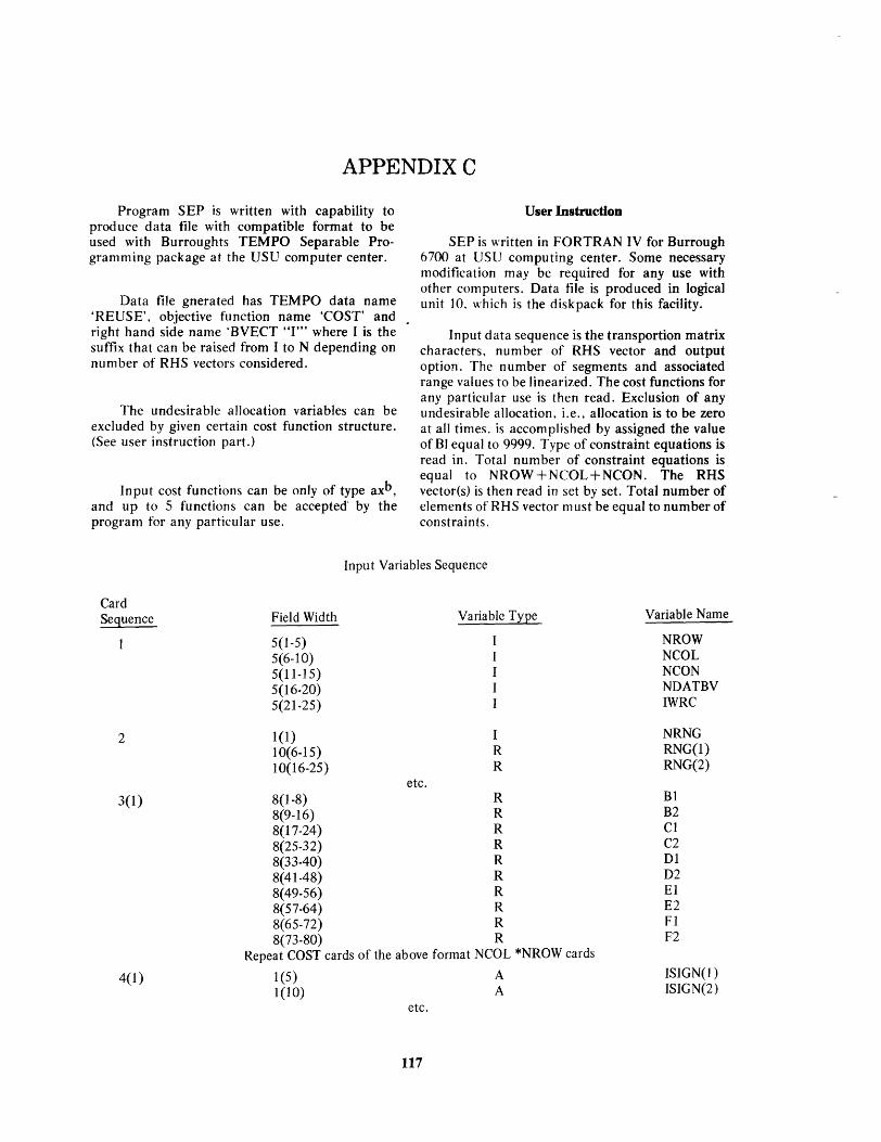
APPENDIXC
Program SEP is written with capability to prod uce data me with compatible format to be used with Burroughts TEMPO Separable Programming package at the USU computer center.
User Instruction
SEP is written in FORTRAN IV for Burrough 6700 at USU computing center. Some necessary modification may be required for any use with other computers. Data file is produced in logical unit to. which is the diskpack for this facility. Data file gnerated has TEMPO data name
'REUSE', objective function name 'COST' and . right hand side name 'BVECT "I'" where I is the suffix that can be raised from I to N depending on number of RHS vectors considered.
Input data sequence is the transportion matrix characters, number of RHS vector and output option. The number of segments and associated range values to be linearized. The cost functions for any particular use is then read. Exclusion of any undesirable allocation, i.e., al1ocation is to be zero at all times, is accomplished by assigned the value of BI equal to 9999. Type of constraint equations is read in. Total number of constraint equations is equal to NROW+NCOL+NCON. The RHS vector(s) is then read in set by set. Total number of elements of RHS vector must be equal to number of constraints.
The undesirable allocation variables can be excluded by given certain cost function structure. (See user instruction part.)
Input cost functions can be only of type axb , and up to 5 functions can be accepted' by the program for any particular use.
Card Sequence
2
3(1)
4(1)
Field Width
5(1 -5) 5(6-10) 5(11-15) 5(16-20) 5(21-25)
1(1) 10(6-15) 10(16-25)
Input Variables Sequence
Variable Type
etc.
I R R
8(1-8) R 8(9-16) R 8(17-24) R 8(25-32) R 8Q34~ R 8(41-48) R 8(49-56) R 8(57-64) R 8(65-72) R 8(73-80) R
Repeat COST cards of the above format NCOL *NROW cards
1(5) A 1(10) A
etc.
117
Variable Name
NROW NCOL NCON NDATBV IWRC
NRNG RNG(1) RNG(2)
Bl B2 Cl C2 DI D2 El E2 Fl F2
ISIGN(I) ISIGN(2)
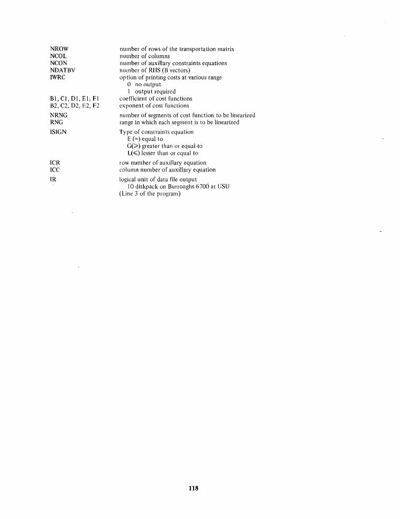
NROW NCOL NCON NOATBV IWRC
Bl, Cl, 01, El, Fl B2,C2,02,E2,F2
NRNG RNG ISIGN
ICR ICC IR
number of rows of the transportation matrix number of columns number of auxillary constraints equations number of RHS (B vectors) option of printing costs at various range
o no output 1 output required
coefficient of cost functions exponent of cost functions
number of segments of cost function to be linearized range in which each segment is to be linearized
Type of constraints equation E (=) equal to G(» greater than or equal.to L(~) lesser than or equal to
row number of auxiliary equation column number of auxillary equation
logical unit of data file output 10 diskpack on Burroughs 6700 at USU
(Line 3 of the program)
118
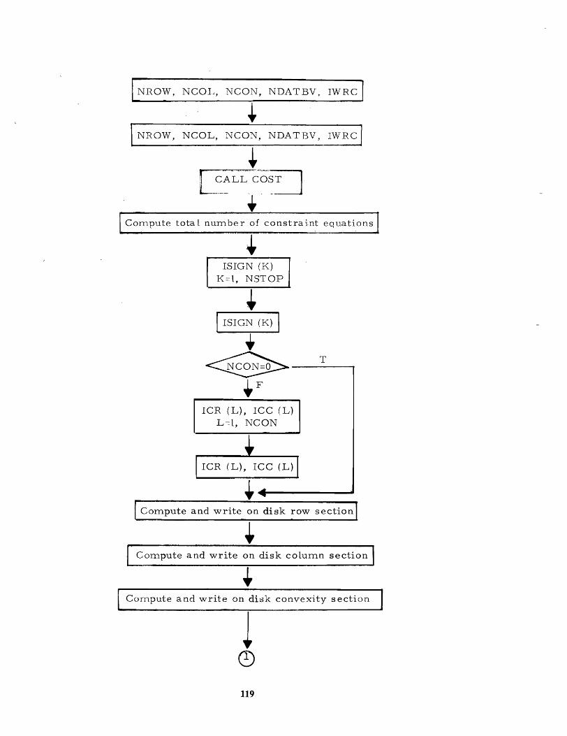
INROW.
\NROW.
Compute
NCOL, NCON, NDATBV,
~ NCOL, NCON, NDATBV,
~ L~~LLCO~
• tota l number of constraint
~ ISIGN (K)
K=l, NSTOP
I ISIGN (K) I
+
IWRC I
IWRCI
equations
~ _____ T __ __
+F ----,
ICR (L), ICC (L) L=l, NCON
+4~~------------~ I Compute and write on disk row section I
+ Cornpute and write on disk coLurnn section
Compute and write on disk convexity section
l Q)
119
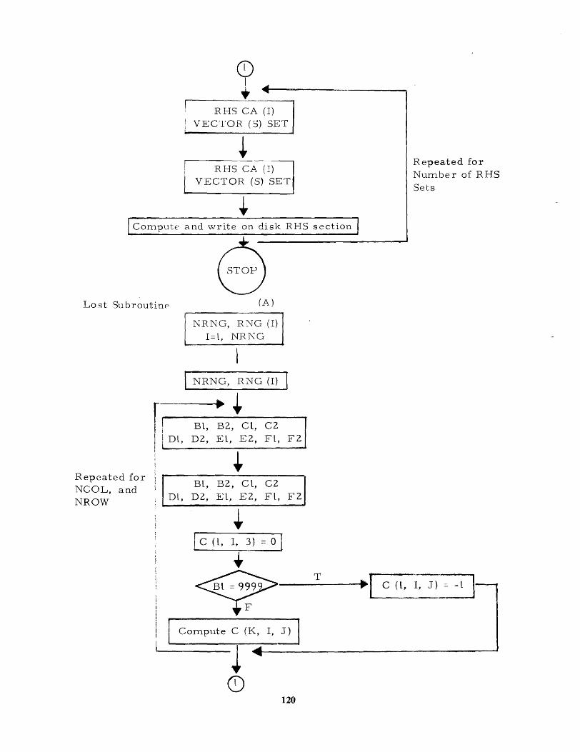
r~ ----RHS CA (I)
VECTOR (S) SET
~~ RHS- CA-(I) I
VECTOR (8) SET'
~
Repeated for Number of RHS Sets
I Compute and write on disk RHS section'
8 La st Su broutine (A)
Repeated for NCOL, and NROW
r I i
! ! Dl, !
: i l
I i
Dl,
NRNG, RNG (I) l=l, NRNG
NRNG, RNG (I)
• ~ Bl, B2, Ct, C2 D2, El, E2, Fl,
+ Bl, B2, C l, C2
DZ, El, E2, Fl,
~ 1 C (l, I, 3) = 0 l
.+
F2
F2
T .. [ C (l, I, J) = -l
I\ll ""'--_--:---_---1 . . Compute C (K, I, J)
~,--__ ---1
<0 120
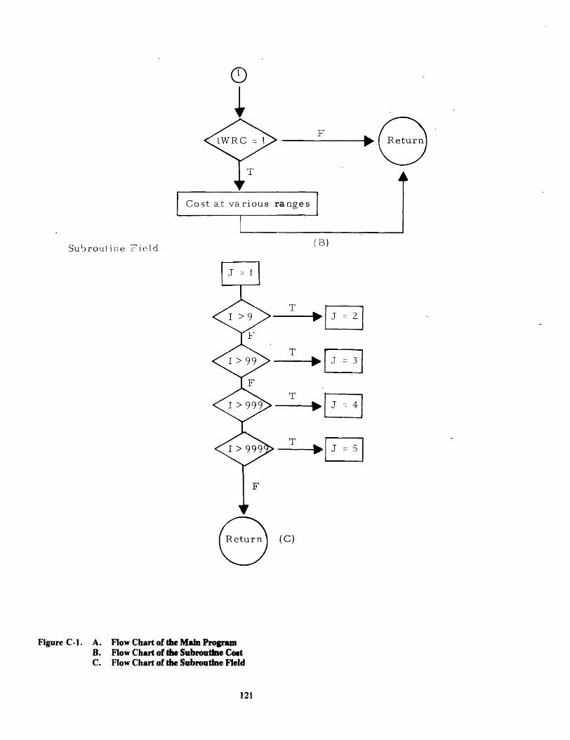
Co st a t va rious ra nge s
Su~rouhne :t-;-'ield ( B)
T
·8 T ·8 T ·8 T ·6
8 (C)
Figure C-l. A. Flow Chart of the Main Propun B. Flow Chart of the Subroutine Colt C. Flow Chart of the Subroutine Field
121
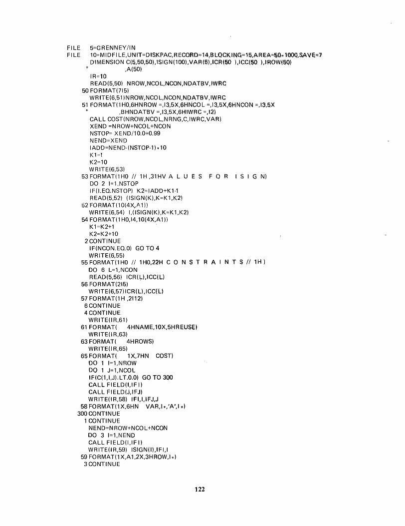
FILE FILE
5=GRENNEY/IN 1 O=IVII D F I LE,UNIT=DISKPAC,RECORQ=14,6 LQCK tNQ==l5,I'\JH~A=~O* lOOQ,S,A VE:;;l DIIVIENSION C(5,50,50),ISIGN(100),VARt~),lCR{5D ).ICC(SO ),IROW(!?'Q}
* ,A(50) IR=10 R EAD(5,50) N ROW ,NCO L,NCON,NDATSV, tWRC
50 FORMAT(715) WRIT E (6,51 ) N ROW, NCO L,N CO N"NOA TBV, IW RC
51 FORMAT(1 HO,6HNROW =,13,5X,6HNCOL =,IS.5X,6HNCON ::i:,13,~X * ,BHNDATBV =,13,5X,6HIWRC =,12)
CALL COST(NROW,NCOL,NRNG,C,IWRC,VAR) XEND=NROW+NCQL+NCON NSTOP= X END/1 0.0+0.99 I\JEND=XEND IADD=NEND-(NSTOP-1)* 10 K 1::::1 K2=10 WR ITE(6,53)
53FORMAT(1HOI11H,31HVALUES FOR ISIGN) DO 2 1=1 ,NSTOP IF(I.EO.NSTOP) K2=IADD+K1-1 READ(5,52) (ISIGN(K),K=K1,K2)
52 FORMAT( 1 0(4X .. .A.1}) WR ITE(6,54) 1,( ISIG N(K) ,K=K 1 ,K2)
54 FORMAT(1 HO,14, 10(4X,A1)) K1=K2+1 K2=K2+10
2CONTINUE IF(NCON.EO.O) GO TO 4 WRITE(6,55)
55 FORMAT(1HO II 1HQ,22H CON S T R A I NT S 1/ 1H) DO 6 L=1,NCON READ(5,56) ICR(L),ICC(L)
56 FORMAT(215) WR ITE(6,57) ICR( U ,leC(U
57 FORMAT(1 H ,2112) 6CONTINUE 4CONTINUE
WRITE(I R,61) 61 FORMAT( 4HNAME,10X,5HREUSE)
WR ITE(I R,63) 63 FORMAT( 4HROWS)
WR ITE( I R,65) 65 FORMAT( 1 X,7HN COST)
DO 1 1=1,NROW DO 1 J=1,NCOL IF(C(1,I,J).LT.0.0) GO TO 300 CALL FIELO(I,IF I) CALL FIELO(J,IFJ) WRITE(IR,58) IFI,I,IFJ,J
58 FORMAT(1 X,6HN VAR,I*,'A',I~)
300 CONTINUE 1 CONTINUE
NENO=NROW+NCOL+NCON DO 3 1=1,I\IENO CALL FIELO(I,IF I) WRITE(IR,59) ISIGN(I),IFI,I
59 FORMAT(1X,A1,2X,3HROW,I*) 3 CONTINUE
122