ABSTRACT

Title of dissertation: DISTRIBUTED OPTIMIZATION OF RESOURCEALLOCATION FOR SEARCH AND TRACKASSIGNMENT WITH MULTIFUNCTION RADARS

Tracie A. Severson, Doctor of Philosophy, 2013

Dissertation directed by: Dr. Derek A. PaleyDepartment of Aerospace Engineeringand the Institute for Systems Research

The long-term goal of this research is to contribute to the design of a concep-

tual architecture and framework for the distributed coordination of multifunction

radar systems. The specific research objective of this dissertation is to apply results

from graph theory, probabilistic optimization, and consensus control to the problem

of distributed optimization of resource allocation for multifunction radars coordi-

nating on their search and track assignments. For multiple radars communicating

on a radar network, cooperation and agreement on a network resource management

strategy increases the group’s collective search and track capability as compared

to non-cooperative radars. Existing resource management approaches for a sin-

gle multifunction radar optimize the radar’s configuration by modifying the radar

waveform and beam-pattern. Also, multi-radar approaches implement a top-down,

centralized sensor management framework that relies on fused sensor data, which

may be impractical due to bandwidth constraints.

This dissertation presents a distributed radar resource optimization approach

for a network of multifunction radars. Linear and nonlinear models estimate the

resource allocation for multifunction radar search and track functions. Interactions

between radars occur over time-invariant balanced graphs that may be directed or

undirected. The collective search area and target-assignment solution for coordi-

nated radars is optimized by balancing resource usage across the radar network and

minimizing total resource usage. Agreement on the global optimal target-assignment

solution is ensured using a distributed binary consensus algorithm. Monte Carlo

simulations validate the coordinated approach over uncoordinated alternatives.

DISTRIBUTED OPTIMIZATION OF RESOURCE ALLOCATIONFOR SEARCH AND TRACK ASSIGNMENT WITH

MULTIFUNCTION RADARS

by

Tracie Andrusiak Severson

Dissertation submitted to the Faculty of the Graduate School of theUniversity of Maryland, College Park in partial fulfillment

of the requirements for the degree ofDoctor of Philosophy

2013

Advisory Committee:Professor Derek A. Paley, Chair/AdvisorProfessor David L. AkinProfessor Balakumar Balachandran, Dean’s RepresentativeProfessor Robert M. SannerProfessor Raymond J. Sedwick

c© Copyright byTracie Andrusiak Severson

2013

Dedication

To Matt and Luke

ii

Acknowledgments

There are many individuals to whom I owe a debt of gratitude for their support

and encouragement during the process of obtaining my Ph.D.

I sincerely thank my advisor, Dr. Derek Paley for giving me the opportunity

to be a graduate student in his laboratory. He was willing to work within the time

constraints imposed by my Navy Permanent Military Professor program as well as

my personal research interests and for that I’m extremely grateful. In addition

to teaching me invaluable skills in effective written communication and rigorous

attention to detail in my research, Derek has taught me the importance of balancing

professional aspirations with family commitments.

A heartfelt thank you to my former advisor at the University of Michigan, Dr.

Dennis Bernstein. I’m excited that our paths have crossed once again after 13 years.

I’m grateful to a number of students in the Collective Dynamics and Control Labo-

ratory. I thank my officemate Levi DeVries for insightful discussions on everything

from cooperative control to crop dusting. To Amanda Chicoli, Nitin Sydney, Frank

Lagor, and Daigo Shishika—thank you for your friendship and encouragement. I’ve

truly enjoyed getting to know you all. Thanks also to former CDCL member Cammy

Peterson for her time and invaluable feedback.

The Navy has been my “home away from home” every since I graduated from

high school. There are many mentors and friends who have played a key role in my

Naval career and especially those who have helped me get to where I am today. I

especially wish to thank RADM (Ret.) Brad Hicks, CAPT (Ret.) Albert Grecco,

iii

CAPT Tim Kelly, CAPT (Ret.) Ronald Crowell, and CAPT Jim Kilby. I hope to

one day exhibit half of the leadership abilities each of you possesses.

My faith, family, and friendships are the bedrock of my support group. To

my dear friends — thank you for giving me the much needed distractions these past

three years. I truly appreciate your genuine interest in my work and even more so

your efforts to get me to away from my computer and outside to breathe in the

fresh air. I thank my parents Gary and Karen for instilling in both their daughters

a sense of integrity and a work ethic that drives us to complete each task we set our

hearts upon. I am truly blessed to call you Mom and Dad. To my in-laws Ray and

Roxie—your kindness and generosity humble me. A special thank you to my sister

Ericka who always understood me before I even spoke.

Without the enduring love and support of my husband Matt and son Luke

I would not have been able to complete this journey. Your sacrifices never went

unnoticed. Thank you for making me feel like the best wife and mother even on

days I had little to offer. I dedicate this dissertation to you.

Lastly I thank God for making all things possible and for always being in

control!

This work was partially funded by the Office of Naval Research under Grant

No. N00174-09-2-00023.

iv

Table of Contents

List of Tables vi

List of Figures vi

List of Abbreviations vii

1 Introduction 1

1.1 Problem Statement . . . . . . . . . . . . . . . . . . . . . . . . . . . . 2

1.2 Relation to Previous Work . . . . . . . . . . . . . . . . . . . . . . . . 5

1.3 Contributions of Dissertation . . . . . . . . . . . . . . . . . . . . . . 8

1.4 Outline of Dissertation . . . . . . . . . . . . . . . . . . . . . . . . . . 10

2 Multifunction Radar Modeling Framework 12

2.1 Radar System Fundamentals . . . . . . . . . . . . . . . . . . . . . . . 13

2.1.1 Detection Probability . . . . . . . . . . . . . . . . . . . . . . . 14

2.1.2 Resource Allocation . . . . . . . . . . . . . . . . . . . . . . . . 15

2.2 Multifunction Radar Model . . . . . . . . . . . . . . . . . . . . . . . 18

2.2.1 Radar Search Function . . . . . . . . . . . . . . . . . . . . . . 18

2.2.2 Target Kinematics . . . . . . . . . . . . . . . . . . . . . . . . 23

2.2.3 Radar Track Function . . . . . . . . . . . . . . . . . . . . . . 26

2.2.4 Target Uncertainty Estimation . . . . . . . . . . . . . . . . . . 27

2.3 Interaction Networks and Consensus Behavior . . . . . . . . . . . . . 32

2.3.1 Graph Theory . . . . . . . . . . . . . . . . . . . . . . . . . . . 32

2.3.2 Radar Communication . . . . . . . . . . . . . . . . . . . . . . 32

2.3.3 Target-Assignment Representation . . . . . . . . . . . . . . . 33

3 Distributed Optimization and Validation in Two Dimensions 37

3.1 Optimization Approach . . . . . . . . . . . . . . . . . . . . . . . . . . 37

3.2 Linear Radar Model . . . . . . . . . . . . . . . . . . . . . . . . . . . 38

3.2.1 Search-Area Maximization . . . . . . . . . . . . . . . . . . . . 40

3.2.2 Target Assignment Optimization . . . . . . . . . . . . . . . . 54

3.3 Nonlinear Radar Model . . . . . . . . . . . . . . . . . . . . . . . . . . 64

3.3.1 Search-Area Maximization . . . . . . . . . . . . . . . . . . . . 65

3.3.2 Target Assignment Optimization . . . . . . . . . . . . . . . . 66

v

4 Consensus-based Optimization and Validation in Three Dimensions 71

4.1 Optimization Approach . . . . . . . . . . . . . . . . . . . . . . . . . . 71

4.2 Target Assignment Optimization . . . . . . . . . . . . . . . . . . . . 74

4.3 Target Assignment Consensus . . . . . . . . . . . . . . . . . . . . . . 79

4.4 Performance Validation . . . . . . . . . . . . . . . . . . . . . . . . . . 82

4.4.1 Scenario 1: Short-range BM Raid . . . . . . . . . . . . . . . . 83

4.4.2 Scenario 2: Medium-range BM Raid . . . . . . . . . . . . . . 86

5 Conclusions 93

5.1 Summary of Dissertation . . . . . . . . . . . . . . . . . . . . . . . . . 93

5.2 Suggestions for Future Research . . . . . . . . . . . . . . . . . . . . . 94

A Search-Area Maximization Analytical Results 97

Bibliography 104

vi

List of Tables

3.1 Analytical Results for N = 3 Ships . . . . . . . . . . . . . . . . . . . 47

3.2 Search-Area Maximization Algorithm . . . . . . . . . . . . . . . . . . 54

3.3 Single Target Assignment Algorithm . . . . . . . . . . . . . . . . . . 59

3.4 Multi-Target Assignment Algorithm . . . . . . . . . . . . . . . . . . . 62

4.1 Genetic Algorithm . . . . . . . . . . . . . . . . . . . . . . . . . . . . 76

4.2 Multifunction Radar Parameters . . . . . . . . . . . . . . . . . . . . . 82

4.3 Scenario 1:Total Missed Targets . . . . . . . . . . . . . . . . . . . . . 86

4.4 Scenario 2:Total Missed Targets . . . . . . . . . . . . . . . . . . . . . 87

List of Figures

1.1 Multi-radar target tracking in a raid scenario . . . . . . . . . . . . . . 3

2.1 Electromagnetic wave propagation . . . . . . . . . . . . . . . . . . . . 14

2.2 Detection probability as a function of SNR . . . . . . . . . . . . . . . 16

2.3 Resource allocation doctrine . . . . . . . . . . . . . . . . . . . . . . . 17

2.4 Resource management implementation . . . . . . . . . . . . . . . . . 18

2.5 Multifunction radar model . . . . . . . . . . . . . . . . . . . . . . . . 22

2.6 Search-area optimization results using SA . . . . . . . . . . . . . . . 23

2.7 Target uncertainty growth . . . . . . . . . . . . . . . . . . . . . . . . 28

2.8 Track quality vs. range to target . . . . . . . . . . . . . . . . . . . . 30

2.9 Communication and target assignment models . . . . . . . . . . . . . 34

3.1 2D linear radar model . . . . . . . . . . . . . . . . . . . . . . . . . . 40

3.2 2D linear Search-area maximization results . . . . . . . . . . . . . . . 42

3.3 Two ship search sector geometry . . . . . . . . . . . . . . . . . . . . . 44

3.4 Three considered scenarios for N = 3 ships . . . . . . . . . . . . . . . 50

3.5 2D linear Target-assignment optimization results . . . . . . . . . . . . 57

3.6 Single-target assignment boundaries . . . . . . . . . . . . . . . . . . . 63

3.7 Multi-target assignment boundaries . . . . . . . . . . . . . . . . . . . 65

3.8 2D nonlinear Search-area maximization . . . . . . . . . . . . . . . . . 67

3.9 2D nonlinear M = 1 target assignment optimization results . . . . . . 69

3.10 Multi-target assignment boundaries . . . . . . . . . . . . . . . . . . . 70

4.1 Consensus behavior . . . . . . . . . . . . . . . . . . . . . . . . . . . . 81

4.2 Launch rate statistics . . . . . . . . . . . . . . . . . . . . . . . . . . . 84

vii

4.3 Scenario 1 BM search sectors and target flight area . . . . . . . . . . 85

4.4 Scenario 1 resource usage statistics . . . . . . . . . . . . . . . . . . . 88

4.5 Scenario 1 mean-centered and worst-case resource usage . . . . . . . . 89

4.6 Scenario 2 BM search sectors and target flight area . . . . . . . . . . 90

4.7 Scenario 2 resource usage statistics . . . . . . . . . . . . . . . . . . . 91

4.8 Scenario 2 mean-centered and worst-case resource usage . . . . . . . . 92

viii

ix

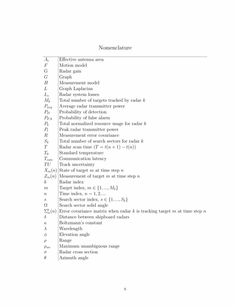
Nomenclature

Ae Effective antenna areaF Motion modelG Radar gainG GraphH Measurement modelL Graph LaplacianLs Radar system lossesMk Total number of targets tracked by radar kPavg Average radar transmitter powerPD Probability of detectionPFA Probability of false alarmPk Total normalized resource usage for radar kPt Peak radar transmitter powerR Measurement error covarianceSk Total number of search sectors for radar kT Radar scan time (T = t(n+ 1)− t(n))T0 Standard temperatureTcom Communication latencyTU Track uncertaintyXm(n) State of target m at time step nZm(n) Measurement of target m at time step nk Radar indexm Target index, m ∈ 1, ...,Mkn Time index, n = 1, 2, ...s Search sector index, s ∈ 1, ..., SkΩ Search sector solid angleΣk

m(n) Error covariance matrix when radar k is tracking target m at time step nδ Distance between shipboard radarsκ Boltzmann’s constantλ Wavelengthφ Elevation angleρ Rangeρun Maximum unambiguous rangeσ Radar cross sectionθ Azimuth angle

x

Chapter 1

Introduction

On July 5th, 2006, The Democratic People’s Republic of Korea (DPRK or

North Korea) reportedly fired at least seven separate ballistic missiles in two rounds

of missile tests [1]. These included one long-range missile and (multiple) short-

range missiles. The long-range Taepodong-2 missile was estimated by United States

intelligence agencies as having a potential range reaching as far as Alaska (although

this missile failed after about 42 seconds of flight). In response to this test and

to other ballistic missile threats, the United States is developing ground- and sea-

based multifunction radar technology to detect and track ballistic missiles of all

ranges—short, medium, intermediate and long [2]. One of the greatest benefits

of a multifunction radar is its ability to simultaneously perform search and track

functions that previously required two or more radars. These functions can be

executed rapidly and independently of one another to support a variety of mission

requirements, such as missile early warning, data collection, and target engagement

support [3],[4]. To facilitate the radar’s ability to manage both its search and track

tasking simultaneously, the radar resource manager must be able to dynamically

vary the radar resource allocation between search and track functions depending

upon the mission objectives and priorities. When the number of targets greatly

exceeds the number of radars (high threat density), the resources required to track

1

each target may exceed each radar’s resource availability. In this situation, missed

target detections and leakers (targets that are detected but not tracked due to

unavailable resources) may occur, especially if the radars are unable to coordinate

on their collective resource allocation.

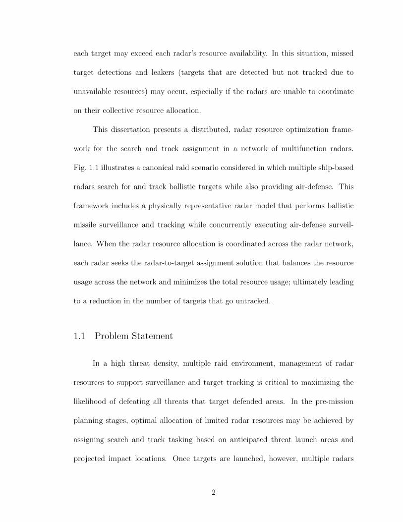
This dissertation presents a distributed, radar resource optimization frame-

work for the search and track assignment in a network of multifunction radars.

Fig. 1.1 illustrates a canonical raid scenario considered in which multiple ship-based

radars search for and track ballistic targets while also providing air-defense. This

framework includes a physically representative radar model that performs ballistic

missile surveillance and tracking while concurrently executing air-defense surveil-

lance. When the radar resource allocation is coordinated across the radar network,

each radar seeks the radar-to-target assignment solution that balances the resource

usage across the network and minimizes the total resource usage; ultimately leading

to a reduction in the number of targets that go untracked.

1.1 Problem Statement

In a high threat density, multiple raid environment, management of radar

resources to support surveillance and target tracking is critical to maximizing the

likelihood of defeating all threats that target defended areas. In the pre-mission

planning stages, optimal allocation of limited radar resources may be achieved by

assigning search and track tasking based on anticipated threat launch areas and

projected impact locations. Once targets are launched, however, multiple radars

2

Figure 1.1: Multi-radar target tracking coordination in a ballistic missile(BM) and air-defense (AD) raid scenario.

may detect and track the same threat, reducing the limited available resources to

search for and detect future targets [5]. While additional radar systems may alleviate

some of the resource burden, a lack of coordination among the participating radars

may still lead to untracked targets due to conflicting resource management priorities.

Cooperation and coordination among a network of mobile maritime multifunc-

tion radars has many advantages. One of the greatest advantages is the ability to

dynamically allocate search and track tasking across the radar network [6],[7]. In

military defense applications, tasking decisions are made so as to increase the col-

lective probability of successfully processing all threats in a high threat density raid

environment. Because resource usage is a function of the instantaneous search and

track tasking, a resource allocation approach that optimizes the collective surveil-

lance area while concurrently optimizing the radar-to-target assignment is needed.

Balancing resource utilization across the radar network prevents a single radar from

3

using all of its available resources unless the other radars are also at or near their

maximum capability. This is important if a majority of the threats are detected

by a subset of radars. Equally important is minimizing the total resource usage

among each radar, allowing for additional resources to be applied either to search

or track functions, depending on the mission priorities as described in a resource

allocation doctrine. Due to the potentially large number of targets, probabilistic ap-

proaches to solving the target-assignment problem, such as genetic algorithms, offer

an alternative method to finding an optimal solution in a reduced timeframe [8].

Because the radars are mobile and often operate in adverse or communications-

denied situations, the resource management framework must be robust to a dynam-

ically changing threat environment that includes the addition or loss of radars to

the network as well as limitations on communications and bandwidth availabil-

ity. A consensus-based distributed (or decentralized ) optimization approach allows

each radar to reach agreement on the optimal target-assignment solution by repeat-

edly exchanging and updating their local target-assignment solutions in an iterative

fashion that yields agreement on a single global solution. In multiagent networks,

consensus means to reach an agreement on a state variable [9], which in our case is

the radar-to-target assignments. A consensus algorithm is an interaction rule that

specifies the information exchange between an agent and all of its neighbors on the

network, typically represented by a graph [9]. Consensus algorithms are guaranteed

to converge even under very mild assumptions on the communication network [10];

indeed, they are tolerant to time-varying, directed communication links [11] and

time-delayed communication [12].

4

The three existing challenges to distributed optimization of resource manage-

ment for multifunction radars addressed in this dissertation are as follows:

1. Construction of a physically representative modeling framework of a multi-

function radar mission that allows a group of radars to coordinate their surveillance

and target-tracking functions.

2. Optimization of the radar resource allocation for a network of coordinated

multifunction radars in a high threat density environment.

3. Demonstration through Monte Carlo simulations of the performance of the

coordinated resource allocation approach verses uncoordinated alternatives.

1.2 Relation to Previous Work

Radar sensing systems provide an attractive platform for sensor management

applications due to their controllable degrees of freedom, such as bandwidth, fre-

quency, sampling rate, and beamform. These characteristics, traditionally hard-

wired into the radar, now allow engineers to design and optimize their configuration

to satisfy a variety of mission requirements by using a resource scheduling policy

that accounts for the radar’s resource constraints. One of the most well-developed

focus applications of resource management for multifunction radar systems is the

application of real-time, closed-loop scheduling of radar resources [13],[5]. Kershaw

and Evans [14], [15] provided some of the earlier work on closed-loop waveform

management for sensor management applications by investigating various adaptive

waveform selection techniques based on single target tracking performance in white

5

Gaussian noise. Sowelam and Tewfix in [16], [17] study the radar management prob-

lem of adaptively selecting a minimal set of radar waveforms to obtain an accurate

reconstruction of the target’s reflectivity. Recent radar management approaches

in the literature address radar waveform scheduling for reducing target angle ac-

curacy [18],[19], target identification [20], target tracking [21], and estimating and

tracking multiple targets [22]. In [23], an interleaving algorithm based on a Hopfield

neural network is used to exploit the radar downtime (the time between transmitted

and received pulses) to increase the number of tracking tasks. While optimizing the

radar waveform scheduling seems extremely appropriate for a single radar platform

or a multi-sensor system managed by a centralized controller with access to real-

time information, its extension to multiple radars communicating over a distributed

network presents some nontrivial challenges such as communication requirements

and bandwidth limitations.

Single radar resource management approaches based on modeling the man-

agement as a decision process presented a new perspective and allowed engineers

to apply the principles of Markov Decision Processes (MDP) and Partially Ob-

served MDP (POMDP). Krishnamurthy [24] devised a radar management strategy

to determine how much radar resource (time) to devote to each target based on a

dynamic prioritization schema that accounts for the current target state estimates.

Nino-Mora and Villar in [25] and La Scala and Moran in [26] formulate the resource

management problem as a MDP and present a target update scheduling policy that

assigns radar resources to reduce target tracking-error variances.

Myopic sensor management polices (i.e., policies that decide the best course of

6

action based upon an immediate reward) such as information-theoretic approaches,

provide a lower complexity alternative to determine the optimal configuration for

multifunction radar systems than policies that look ahead to a future reward. While

future radar performance may be sacrificed by only considering its near-term state,

in certain situations myopic scheduling policies may prove more robust to inaccurate

sensor models and dynamic performance objectives. Khosla and Guillochon in [27]

present an information-theoretic approach in which each target has a kinematic

state and target class; sensors can observe either state or class (or both) depending

upon which mode maximizes the information gained on the target. Sinno and Kre-

ithen [28] present a cooperative surveillance and multi-target tracking optimization

approach that maximizes the aggregate Signal-to-Noise Ratio (SNR) for all targets

and minimizes target uncertainty. Kalandros and Pao in [29] use covariance control

to determine the sensor(s) tracking resource allocation in order to reduce the tar-

get state uncertainty. Kreucher et al. in [30] present a sensor management scheme

that maximizes the expected gain in information based on computing the Renyi

Information Divergence [31].

Algorithms that utilize centralized planning nodes for multi-agent coordina-

tion demonstrate quicker search-area coverage and target neutralization than un-

coordinated agents as described by Schumacher et.al in [32]. However restricted

communications and processing resources pose significant challenges to a central-

ized sensor fusion center that receives and processes raw sensor data. When the

expected target locations are unknown, optimization algorithms described by Smith

and Bullo [33],[34] demonstrate detection of a group of distinct target locations

7

within a prescribed environment without assuming exact target coordinates.

For multiple ship-based radars considering a large number of targets, Kang

and Lee [35] divide the radar search sectors such that the relative residual radar

resource capacity is balanced and assign tracking responsibilities based on expected

target arrivals to minimize target migrations from one ship’s search sector to another

ship’s sector. While this approach preserves important target state information by

minimizing migrations, it prevents a radar from tracking targets outside its own

search sector, which may be beneficial in balancing the resource load; it also fails

to address the situation when the tracking resources exceed resources available for

search tasks. Distributed resource management approaches for several multifunc-

tion radars that combine resource minimization with information maximization are

presented by Weir in [6] and Lambert and Sinno in [36] using emergent behavior

and self-organization techniques.

1.3 Contributions of Dissertation

This dissertation applies results from graph theory, probabilistic optimization,

and consensus control to the problem of distributed resource management for coor-

dinated multifunction radars. Specific contributions are described below.

Multifunction radar system model Radar resource allocation is modeled us-

ing a physically representative, three-dimensional, nonlinear framework. Resources

are consumed as each radar searches for, detects, and tracks ballistic missile (BM)

8

targets while concurrently executing air-defense (AD) surveillance requirements. Re-

sources for engagements are modeled using an estimate of the resources required to

reduce the track uncertainty to meet a prescribed engagement requirement.

Optimization of radar resource allocation A distributed approach optimizes

both the collective surveillance area and radar-to-target assignment solution for mul-

tiple radars coordinating over a directed network. The radar-to-target-assignment

problem for coordinated radars is solved by balancing radar resource usage and min-

imizing total radar resource utilization while simultaneously optimizing the limited

search resources by maximizing the search area around the expected target arrival.

The air defense strategy also maximizes the area of each radar’s search sector, which

is centered on an expected threat axis, and ensures that each search sector degrades

symmetrically about the threat axis under heightened track demand.

Consensus-based coordination A distributed consensus algorithm reaches agree-

ment on the single global target-assignment solution. The consensus algorithm

provides robustness to inaccurate or unaccounted for sensor biases, eliminates the

possibility that a detected target is untracked when tracking resources are available,

and ensures that all radars share the same target-assignment solution even in the

presence of communication noise.

Performance validation Monte Carlo simulations demonstrate that a decentral-

ized consensus-based approach to reaching the global optimal radar-to-target as-

9

signment solution allows for a greater number of targets to be detected and tracked

while preserving adequate resources for AD search. The coordinated approach de-

scribed here permits each radar and its local resource manager to maintain control

over its resource allocation subject to the consensus of the radar communication

network. Results are compared to uncoordinated approaches using various existing

resource allocation doctrines in order to highlight the increase in tracked targets

and conservation of radar resources.

1.4 Outline of Dissertation

The outline of this dissertation is as follows.

Chapter 2 presents a physically-representative three-dimensional nonlinear

model of a multifunction radar system, including models of radar detection, surveil-

lance, target tracking, and target uncertainty. It reviews some fundamental proper-

ties of algebraic graph theory and consensus and describes their application to radar

communication and target-assignment networks.

Chapter 3 applies a probabilistic optimization approach for maximizing the

collective search-area of multiple radars coordinating over a directed network using

simplified two-dimensional linear and nonlinear radar models as a first look at multi-

radar resource management. The optimal target-assignment solution in the case of

single or multiple targets in a linear resource usage model has target-assignment

boundaries that are hyperbolic.

Chapter 4 describes an optimization framework for multiple three-dimensional

10

nonlinear radars coordinating over a strongly connected, balanced communication

network with possibly directed links. Section 4.2 solves for the optimal radar-to-

target-assignment, as represented by the adjacency matrix of the target assignment

graph, using a binary genetic algorithm that balances radar resource tasking and

minimizes total radar resource usage. Section 4.3 presents a distributed consensus-

based approach for reaching agreement on the optimal target-assignment, adopting

a binary consensus algorithm following [37] that is robust to communication noise

and fading channels. The multifunction radar resource optimization approach is

validated via Monte Carlo simulations in Section 4.4 and compared to two uncoor-

dinated approaches for both a short range and medium range ballistic missile radar

mission.

Chapter 5 summarizes the dissertation and provides suggestions for future

research.

11

Chapter 2

Multifunction Radar Modeling Framework

A multifunction radar system performs a variety of functions originally as-

signed to multiple radars. Shipboard multifunction radars support surface search,

air-defense search, ballistic missile search, ballistic missile tracking, and air-defense

tracking [38]. Because the execution of each function is separable, the radar signal

and data processing applied to each function can be controlled and optimized given

the overall mission objectives [39]. While there are a variety of (oftentimes com-

peting) objectives, the primary goal of this dissertation is to optimize the resource

allocation for ballistic missile and air-defense search and track functions to increase

the number of tracked ballistic missile targets.

This chapter presents the multifunction radar, communication, and target-

assignment network models used in the multi-target search and track optimization

approach. Section 2.1 reviews some fundamental properties of multifunction radar

systems and resource management implementations, including the resource alloca-

tion doctrine. Section 2.2 introduces the search and track resource allocation models

as well as the ballistic missile target kinematic model. Motivated by the radar’s po-

tential requirement to support a weapon’s engagement, this section also describes

a method to assess the performance of the target tracking system in terms of the

track uncertainty and how this uncertainty estimate is incorporated in the radar re-

12

source model. Section 2.3 reviews some fundamental properties of graphs and their

application to sensor networks and communication models including consensus.

2.1 Radar System Fundamentals

Radars operate by emitting electromagnetic energy in the form of an electro-

magnetic wave. Some of that energy is scattered due to the wave’s interaction with

the environment while a smaller portion of the scattered energy, called the radar

echo, is collected by the receiving radar antenna (see Fig. 2.1). The time difference

τ between when the pulse of electromagnetic energy is transmitted and when the

target echo is received is proportional to the target range ρ, given by [4]

τ =2ρ

c, (2.1)

where c is the speed of the electromagnetic wave propagation. The pulse repetition

interval (PRI) specifies the time interval between successive pulses and is inversely

proportional to the pulse repetition frequency (PRF), where PRF = 1/(PRI).

Because of the time delay between when a radar pulse is transmitted and when the

radar echo is received, range ambiguities may occur when it is not clear from which

of the transmitted pulses the received echo originated. The maximum unambiguous

range ρun is proportional to the pulse repetition interval, i.e., [38]

ρun =c(PRI)

2. (2.2)

13

AntennaTransmitted Signal Received Signal Target

Range(ρ)

Figure 2.1: Received radar echo attenuated due to interaction with a target and theenvironment.

The duty cycle of a radar specifies the fraction of time that the radar system

is in an “active” state, i.e., the portion of time the system is operational. The

duty cycle is used to calculate both the peak power Pt and average power Pavg of a

particular radar system, [4]

Duty Cycle =PavgPt

. (2.3)

2.1.1 Detection Probability

A multifunction radar system produces range, doppler, and angle measurement

data. In order to determine the presence of targets, signal processing is applied to

the measurement data to differentiate between a target present hypothesis (H1) and

target not present hypothesis (H0). Receiver background and thermal noise fluc-

tuations complicates the decision process. The detection performance, Probability

of Detection (PD), depends upon the strength of the returned target signal relative

to that of the noise (Signal to Noise Ratio) and threshold setting (Probability of

False Alarm). The Neyman-Pearson criterion [40] says that the decision rule should

be constructed to maximize the Probability of Detection while not allowing the

14

Probability of False Alarm to exceed a certain value,

maxPD, such that PFA ≤ α. (2.4)

The solution to the optimization problem in 2.4 is given by the Neyman-Pearson

lemma [41], which defines the optimal decision region for a fixed probability of false

alarm PFA as a threshold η on likelihood ratio LR for measurement vector X [39]:

LR(X) =p(X|H1)

p(X|H0)

H1

><

H0

η (2.5)

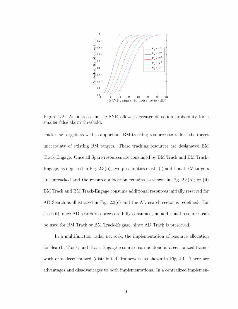
where η is chosen such that PFA = p(X > η|H0). For a minimum probability

of detection and a maximum probability of false alarms, the Signal to Noise ratio

(SNR) can be computed using Albersheim’s equation [4], which provides a closed-

form approximation of the SNR required for non-fluctuating targets in independent

and identically distributed Gaussian noise (see Fig. 2.2).

2.1.2 Resource Allocation

Consider a network of identical multifunction radars that search for and track

ballistic missiles (BM) while also performing air defense (AD) search. Each radar

has the same maximum resource allocation and a fixed location. The initial re-

source allocation is partitioned into AD Search, AD Track, BM Search, BM Track,

and Spare as shown in Fig. 2.3(a). As BM targets are detected and tracking as-

signments determined, BM Track consumes resources initially designated Spare to

15

0 5 10 15 20 25 30 350.1

0.2

0.3

0.4

0.5

0.6

0.7

0.8

0.9

1

(S/N )1, signal to noise ratio (dB)

Pro

bababil

tyof

det

ecti

on

Pfa = 10 3

Pfa = 10 4

Pfa = 10 5

Pfa = 10 6

Pfa = 10 7

Figure 2.2: An increase in the SNR allows a greater detection probability for asmaller false alarm threshold.

track new targets as well as apportions BM tracking resources to reduce the target

uncertainty of existing BM targets. These tracking resources are designated BM

Track-Engage. Once all Spare resources are consumed by BM Track and BM Track-

Engage, as depicted in Fig. 2.3(b), two possibilities exist: (i) additional BM targets

are untracked and the resource allocation remains as shown in Fig. 2.3(b); or (ii)

BM Track and BM Track-Engage consume additional resources initially reserved for

AD Search as illustrated in Fig. 2.3(c) and the AD search sector is redefined. For

case (ii), once AD search resources are fully consumed, no additional resources can

be used for BM Track or BM Track-Engage, since AD Track is preserved.

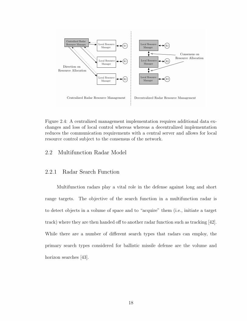
In a multifunction radar network, the implementation of resource allocation

for Search, Track, and Track-Engage resources can be done in a centralized frame-

work or a decentralized (distributed) framework as shown in Fig 2.4. There are

advantages and disadvantages to both implementations. In a centralized implemen-

16

tation, a central radar resource manager receives all search and track information

from participating local resource managers and makes informed decisions based on

global knowledge. These decisions are broadcast as directives to the local resource

managers for execution and in theory should be optimal as compared to some per-

formance objective based on full knowledge of the situation. The drawbacks to a

Spare

AD

Tra

ck

AD

Sea

rch

BM

Sear

ch

BMTrac

k

(a) Initial

BM Track +BM Track-Engage

AD

Tra

ck

AD

Sea

rch

BM

Sear

ch

(b) Fixed

AD

Tra

ck

AD

Sea

rch

BM

Sear

ch

BM Track +BM Track-Engage

(c) Variable

Figure 2.3: The radar resource manager will dynamically allocate finite availablesearch and track resources to accomplish mission objectives and maximize systemperformance.

centralized implementation are the increased data exchange requirements between

the local and central resource manager as well as a loss of local control at the radar

level.

In contrast to a centralized resource management implementation, a distributed

implementation allows each local radar resource manager to decide on the optimal

resource management policy and then reach agreement on the global policy through

the process of consensus. In this implementation, each local resource manager main-

tains control of their resource allocations subject to the consensus of the network.

It also significantly reduces the information exchange requirements over an already

bandwidth-constrained communication link.

17

R1

R2

R3Local Resource

Manager

Local ResourceManager

Local ResourceManager

Centralized RadarResource Manager

R1

R2

R3Local Resource

Manager

Local ResourceManager

Local ResourceManager

Centralized Radar Resource Management Decentralized Radar Resource Management

Direction onResource Allocation

Consensus onResource Allocation

Figure 2.4: A centralized management implementation requires additional data ex-changes and loss of local control whereas whereas a decentralized implementationreduces the communication requirements with a central server and allows for localresource control subject to the consensus of the network.

2.2 Multifunction Radar Model

2.2.1 Radar Search Function

Multifunction radars play a vital role in the defense against long and short

range targets. The objective of the search function in a multifunction radar is

to detect objects in a volume of space and to “acquire” them (i.e., initiate a target

track) where they are then handed off to another radar function such as tracking [42].

While there are a number of different search types that radars can employ, the

primary search types considered for ballistic missile defense are the volume and

horizon searches [43].

18

Volume Search

A volume search is a 360 search patten [44] that covers the area around the

sensor out to a defined range [44]. This type of search is used for radars operating in

air defense applications such as the search and tracking of aircraft, cruise missiles,

and UAVs where targets can originate from multiple directions. The downside of a

volume search is the large amount of radar resources required to cover the full volume

and therefore the relatively large amount of time to complete a search pattern. To

reduce the time required to search the volume, the detection range can be reduced,

however this impacts the long-range performance required for the ballistic missile

defense mission [45].

To prevent range degradation for ballistic missile performance, a search sec-

tor is defined by its range, azimuth, and elevation, creating a volume search on a

well-defined area. In addition to the characteristics above, a volume search is also

specified by the time Tsearch required to execute the search, the allowed false-alarm

rate PFA, and the desired probability of detection PD.

Horizon Search Fence

In contrast to a volumetric search, the horizon search utilizes only a single

row of beams at or above the horizon for search and acquisition applications [42].

This search is commonly used for early warning missile surveillance radars as well

as ballistic missile defense radars and operates under the assumption that for an

adequate detection range, any ascending ballistic target must fly through the fence

19

and thus will be detected.

Resource Model

The Signal to Noise ratio (SNR) is the standard measure of a radar’s ability to

detect a given target at a range ρ from the radar [44]. SNR is a linear function of the

inverse search sector solid angle1 Ω and a quartic function of the inverse detection

range ρ [4, pp. 30-90]:

SNR =PavgAeσTsearch4πκT0Lsρ4Ω

, (2.6)

where Pavg is the average transmitted power, Ae is the effective antenna area, σ is

the target radar cross section, κ is Boltzmann’s constant, T0 is the radar system

temperature, Ls are the total system losses, and Tsearch is the search scan time for

solid angle Ω at range ρ. Radar resource usage is expressed in units of time by

solving 2.6 for the search scan time Tsearch, which yields

Tsearch = aρ4Ω, (2.7)

where

a , 4πκT0(SNR)Ls/(PavgAeσ) (2.8)

is considered identical for all radars. To avoid unnecessary complexity, the radar

model performs search tasks uniformly so that resources are equally distributed

among each of the search directions in Ω.

1The solid angle subtended by a surface is the surface area of the portion of a unit spherecovered by the surface’s radial projection onto the sphere [46].

20

For a particular radar system design and expected target surveillance mission,

the parameters of 2.8 are assumed to be known and fixed. In the event of multiple

search sectors, let Sk represent the total number of ballistic missile and air-defense

search sectors for radar k. The total search scan time T(tot)search,k dedicated to searching

all Sk sectors of radar k is expressed as

T(tot)search,k = a

Sk∑s=1

ρ4s,kΩs,k, (2.9)

where s ∈ 1, ..., Sk is the search sector index.

In many surveillance missions the potential threat axis is known (i.e., the most

probable direction from which a target will arrive). The search sector is typically

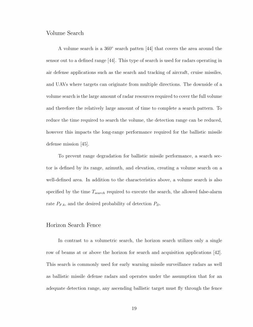
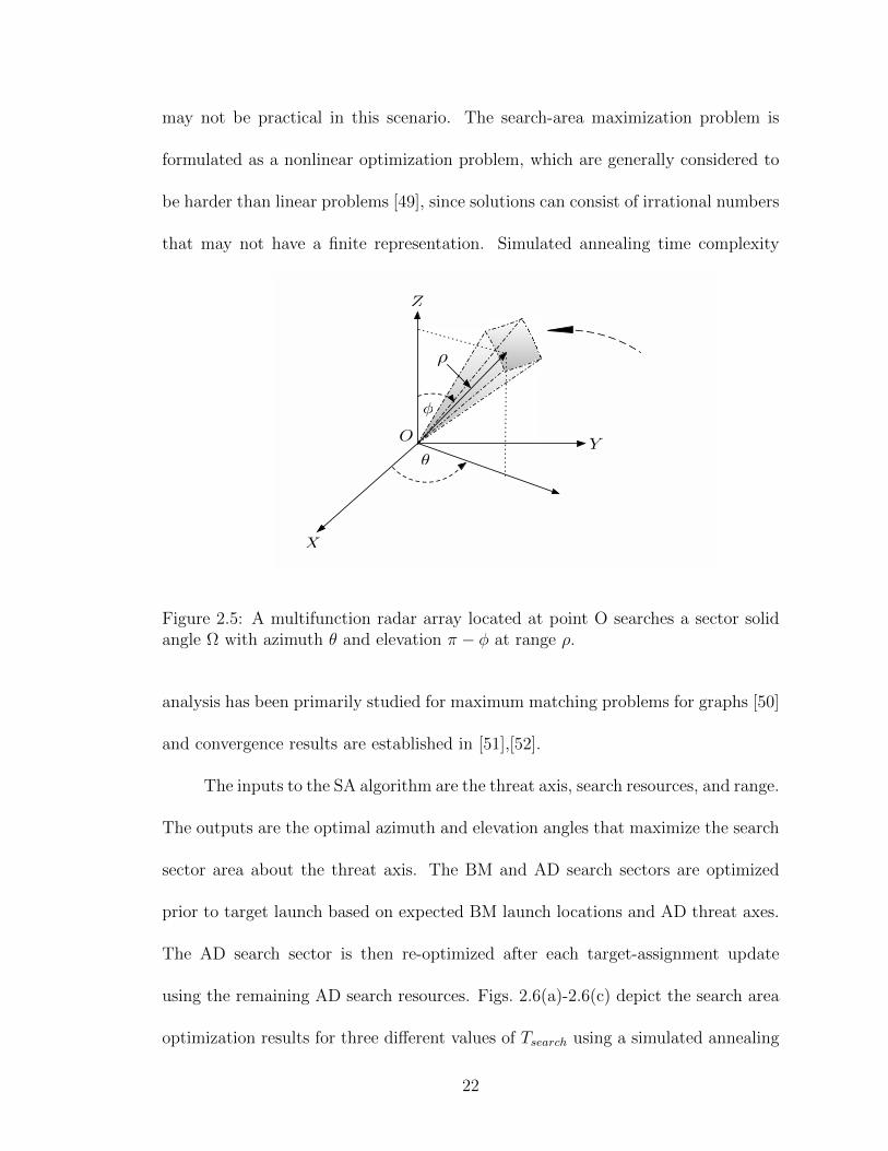
centered on this threat axis and its surface area maximized. Fig. 2.5 illustrates the

geometry required for computing the surface area A and solid angle Ω. The surface

area A of a spherical sector bounded by azimuth angles (θ1, θ2) and elevation angles

(φ1, φ2) is

A = ρ2(θ2 − θ1)(cosφ2 − cosφ1). (2.10)

Dividing 2.10 by ρ2 gives the solid angle [46] Ω = (θ2 − θ1)(cosφ2 − cosφ1).

The surface area in 2.10 is maximized along a potential threat axis at a given

range ρ using a fast, numerical heuristic known as simulated annealing [47] (SA). A

simulated annealing algorithm is employed to solve this optimization problem even

though it is not guaranteed to find the global optimum, because it is significantly

more computationally efficient than exhaustive search strategies [48, Ch. 3], which

21

may not be practical in this scenario. The search-area maximization problem is

formulated as a nonlinear optimization problem, which are generally considered to

be harder than linear problems [49], since solutions can consist of irrational numbers

that may not have a finite representation. Simulated annealing time complexity

X

Y

Z

φ

ρ

θ

O

Figure 2.5: A multifunction radar array located at point O searches a sector solidangle Ω with azimuth θ and elevation π − φ at range ρ.

analysis has been primarily studied for maximum matching problems for graphs [50]

and convergence results are established in [51],[52].

The inputs to the SA algorithm are the threat axis, search resources, and range.

The outputs are the optimal azimuth and elevation angles that maximize the search

sector area about the threat axis. The BM and AD search sectors are optimized

prior to target launch based on expected BM launch locations and AD threat axes.

The AD search sector is then re-optimized after each target-assignment update

using the remaining AD search resources. Figs. 2.6(a)-2.6(c) depict the search area

optimization results for three different values of Tsearch using a simulated annealing

22

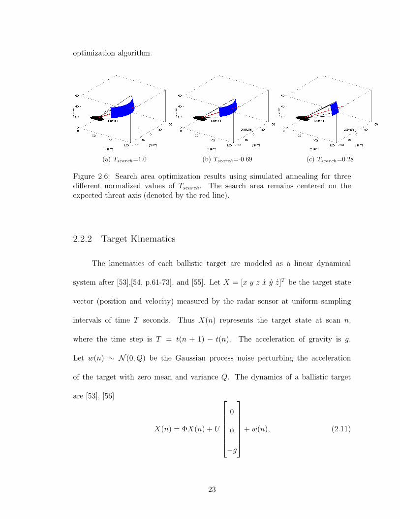
optimization algorithm.

(a) Tsearch=1.0 (b) Tsearch=-0.69 (c) Tsearch=0.28

Figure 2.6: Search area optimization results using simulated annealing for threedifferent normalized values of Tsearch. The search area remains centered on theexpected threat axis (denoted by the red line).

2.2.2 Target Kinematics

The kinematics of each ballistic target are modeled as a linear dynamical

system after [53],[54, p.61-73], and [55]. Let X = [x y z x y z]T be the target state

vector (position and velocity) measured by the radar sensor at uniform sampling

intervals of time T seconds. Thus X(n) represents the target state at scan n,

where the time step is T = t(n + 1) − t(n). The acceleration of gravity is g.

Let w(n) ∼ N (0, Q) be the Gaussian process noise perturbing the acceleration

of the target with zero mean and variance Q. The dynamics of a ballistic target

are [53], [56]

X(n) = ΦX(n) + U

0

0

−g

+ w(n), (2.11)

23

where

Φ=

1 0 0 T 0 0

0 1 0 0 T 0

0 0 1 0 0 T

0 0 0 1 0 0

0 0 0 0 T 0

0 0 0 0 0 T

and U=

T 2/2 0 0 T 0 0

0 T 2/2 0 0 T 0

0 0 T 2/2 0 0 T

T

. (2.12)

The measurements collected by a radar at the uniform time intervals T are

the range ρ, the azimuth θ, and elevation φ, subject to measurement noise with

variance σ2ρ, σ

2θ , and σ2

φ, respectively. Let (xk, yk, zk) be the location of radar k.

The relationships between the radar measurements and the target state are [57, pp.

46],[58, pp. 54]

ρ = [(x− xk)2 + (y − yk)2 + (z − zk)2]1/2

θ = arctan

(x− xky − yk

)φ = arcsin

(z − zkρ

). (2.13)

The (nonlinear) measurement equation is

Z(n) = h(X(n)) + v(n), (2.14)

where Z = [ρ θ φ]T and v ∼ N (0, S) is the zero mean uncoupled measurement error

24

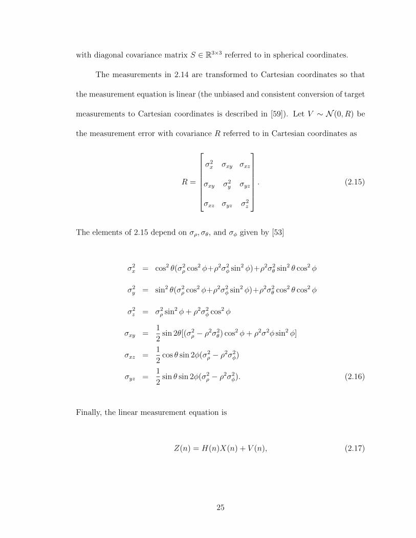
with diagonal covariance matrix S ∈ R3×3 referred to in spherical coordinates.

The measurements in 2.14 are transformed to Cartesian coordinates so that

the measurement equation is linear (the unbiased and consistent conversion of target

measurements to Cartesian coordinates is described in [59]). Let V ∼ N (0, R) be

the measurement error with covariance R referred to in Cartesian coordinates as

R =

σ2x σxy σxz

σxy σ2y σyz

σxz σyz σ2z

. (2.15)

The elements of 2.15 depend on σρ, σθ, and σφ given by [53]

σ2x = cos2 θ(σ2

ρ cos2 φ+ρ2σ2φ sin2 φ)+ρ2σ2

θ sin2 θ cos2 φ

σ2y = sin2 θ(σ2

ρ cos2 φ+ρ2σ2φ sin2 φ)+ρ2σ2

θ cos2 θ cos2 φ

σ2z = σ2

ρ sin2 φ+ ρ2σ2φ cos2 φ

σxy =1

2sin 2θ[(σ2

ρ − ρ2σ2θ) cos2 φ+ ρ2σ2φ sin2 φ]

σxz =1

2cos θ sin 2φ(σ2

ρ − ρ2σ2φ)

σyz =1

2sin θ sin 2φ(σ2

ρ − ρ2σ2φ). (2.16)

Finally, the linear measurement equation is

Z(n) = H(n)X(n) + V (n), (2.17)

25

where Z = [x y z]T and

H =

1 0 0 0 0 0

0 1 0 0 0 0

0 0 1 0 0 0

. (2.18)

Because 2.11 and 2.17 are both linear with w(n) and V (n) additive white noise

Gaussian processes, a Kalman filter provides the optimal (in the minimum mean-

squared sense) unbiased estimate of the target state vector.

2.2.3 Radar Track Function

Once a target is detected and track initiation completed, the radar array beam

is steered directly to the target [4],[38] for track updates, thus

SNR =PtG

2λ2σTtrack(4π)3κT0Lsρ4

, (2.19)

where Pt is the peak transmitter power, G is the antenna gain, λ is the wavelength,

and Ttrack is the amount of time the target is in track. Solving for Ttrack we have

Ttrack = cρ4, (2.20)

where

c , (4π)3κT0(SNR)Ls/(PtG2λ2σ). (2.21)

26

Let Mk be the number of targets tracked by radar k so that the total target track

time for radar k can be expressed as

T(tot)track,k = c

Mk∑m=1

ρ4m,k (2.22)

where m = 1, ...,Mk is the target index.

2.2.4 Target Uncertainty Estimation

A measure of track uncertainty is required by many weapon systems to assess

the performance of the target tracking system as well as aid in sensor resource alloca-

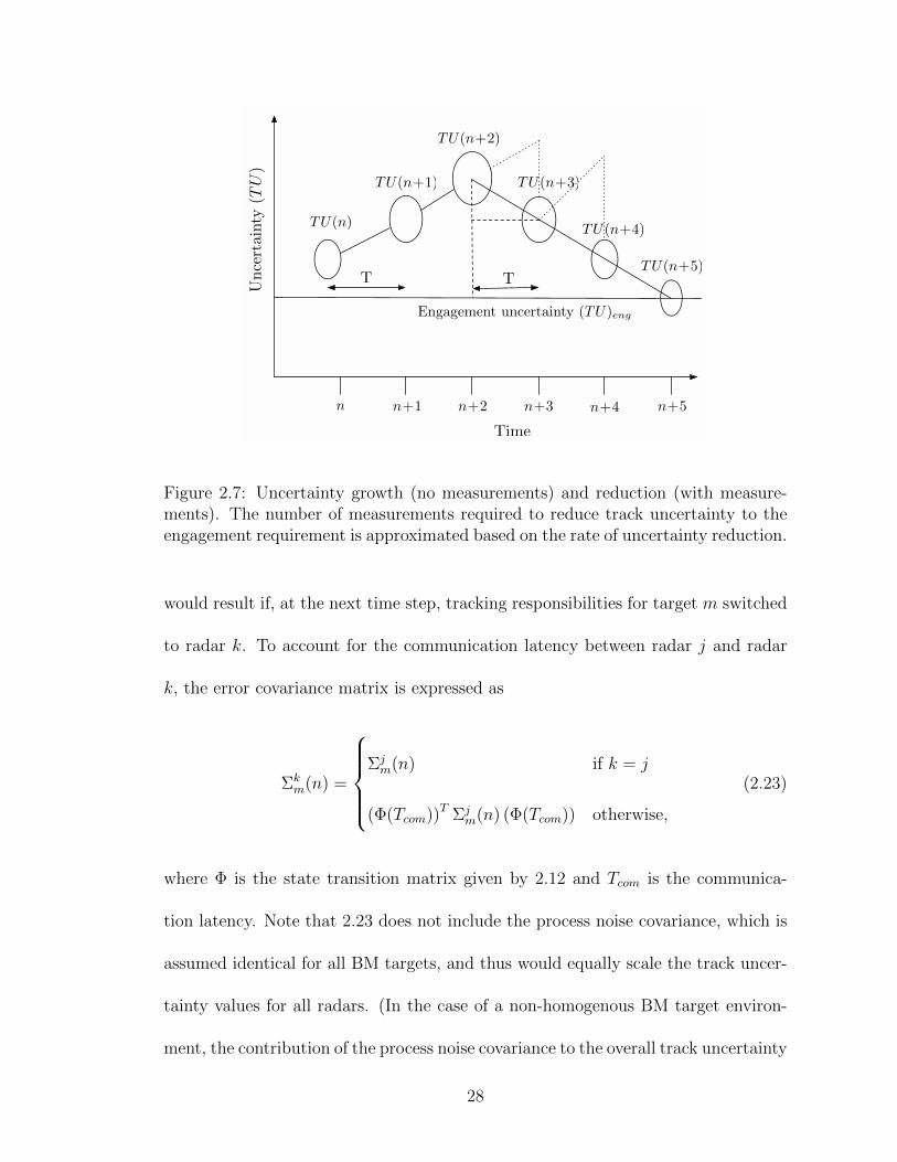
tion decisions to satisfy the demands of engagement [36],[43],[58, pp. 168]. Fig. 2.7

illustrates how target uncertainty grows over time in the absence of measurements.

Successive measurement updates can reduce the target state uncertainty to meet an

engagement performance requirement, provided the target update rate is sufficient.

In [36] and [60], sensors compute their contribution to a target state estimate based

on the reduction in estimate uncertainty. Motivated by this work, the projected

reduction in target uncertainty for each radar-target pairing is found based upon

the outputs of a minimum variance linear tracking filter. This value is then used to

approximate the radar resource requirement (number of measurement updates) to

reduce the target uncertainty to a specified level to support an engagement.

Suppose radar j is tracking target m at time step n. Let xm(n) represent the

target state estimate and Σjm(n) be the 6×6 error covariance. For each radar k that

can track target m, let Σkm(n + 1) represent the 6× 6 error covariance matrix that

27

TU(n)

TU(n+1)

TU(n+2)

TU(n+3)

TU(n+4)

TU(n+5)

Time

Unce

rtai

nty

(TU

)

T T

n n+1 n+2 n+3 n+4 n+5

Engagement uncertainty (TU)eng

Figure 2.7: Uncertainty growth (no measurements) and reduction (with measure-ments). The number of measurements required to reduce track uncertainty to theengagement requirement is approximated based on the rate of uncertainty reduction.

would result if, at the next time step, tracking responsibilities for target m switched

to radar k. To account for the communication latency between radar j and radar

k, the error covariance matrix is expressed as

Σkm(n) =

Σjm(n) if k = j

(Φ(Tcom))T Σjm(n) (Φ(Tcom)) otherwise,

(2.23)

where Φ is the state transition matrix given by 2.12 and Tcom is the communica-

tion latency. Note that 2.23 does not include the process noise covariance, which is

assumed identical for all BM targets, and thus would equally scale the track uncer-

tainty values for all radars. (In the case of a non-homogenous BM target environ-

ment, the contribution of the process noise covariance to the overall track uncertainty

28

can be accounted for by adding an additional term (Φ(Tcom))T Qjm(n) (Φ(Tcom))

to 2.23.)

The projected estimate of the Kalman gain at time step n+ 1 if radar k were

assigned tracking responsibilities for target m is

Kkm(n+ 1) = Σk

m(n)HT[HΣk

m(n)HT +Rkm(n+ 1)

]−1, (2.24)

where the measurement error covariance Rkm depends on the position of target m

relative to radar k as given in 2.15. The projected state covariance matrix for radar

k and target m at time step n+ 1 is then

Σkm(n+ 1) =

(I −Kk

m(n+ 1)H)

Σkm(n), (2.25)

where I is the 6× 6 identity matrix. The track uncertainty for each radar-to-target

pairing is computed by summing the diagonal position elements of the covariance

matrix in 2.25 to obtain

(TU)km(n) = Tr[ΦTΣkm(n)Φ]. (2.26)

(The appearance of Φ in 2.26 ensures the units of TU are km2.) Fig. 2.8(a) plots the

trajectory of a single BM target that is launched from the origin and the locations

of four radars. Fig. 2.8(b) depicts the value of the track uncertainty (TU)km(n +

1) for each radar k ∈ 1, 2, 3, 4 assuming a communication latency of Tcom = 6

seconds [60]. The track uncertainty varies according to range and azimuth to the

29

target, so that Radar 4 does not always provide the smallest track uncertainty

despite being closest to the target.

0100

200300

400500 −500

0

500

0

50

100

150

200

y (km)

Radar3

Radar4

Radar1

Radar2

x (km)

z(k

m)

(a) BM trajectory

200 300 400 500 600 700 8001.5

2

2.5

3

3.5

4

4.5

5

5.5

Range (km)

TU

(km

2)

Radar 1

Radar 2

Radar 3

Radar 4

(b) Track Uncertainty

Figure 2.8: (a) Location of N = 4 radars relative to a single BM target that launchesfrom (0,0,0); (b) Track uncertainty is not always minimized by the closest radar.

The engagement track uncertainty, (TU)eng, may be specified in support of

BM and AD engagements; the resources required to reach a desired (TU)eng are

computed using a linear interpolation between the current target uncertainty and the

projected uncertainty at the next time step. Let (TU)km(n) be the track uncertainty

for radar k and target m at time step n using 2.26 with Σkm(n) given by 2.25 and let

(TU)km(n + 1) be the projected track uncertainty for radar k and target m at time

step n + 1. Then the rate of change in track uncertainty between consecutive time

steps is

∆(TU)km = (TU)km(n)− (TU)km(n+ 1) (2.27)

as shown in Fig. 2.2. Let Tmeng,k be the time required for radar k to achieve a desired

track uncertainty on target m. Under a linear approximation, the rate of change in

30

track uncertainty, ∆(TU)km, remains constant so that

Tmeng,k =(TU)km(n)− (TU)eng

∆(TU)kmTtrack,k =

(TU)km(n)− (TU)eng(TU)km(n)− (TU)km(n+ 1)

Ttrack,k. (2.28)

Let Mk be the total number of targets that may be tracked by radar k so that the

total target engagement time is

T(tot)eng,k = c

Mk∑m=1

Tmeng,k. (2.29)

Combining 2.9, 2.20, and 2.29 yields the total resources in units of time required

to complete the desired search and track functions of radar k and to meet the

engagement requirements of all Mk targets. The total resource usage must satisfy

T(tot)search,k + T

(tot)track,k + T

(tot)eng,k + εk ≤ Tmax, (2.30)

where εk represents the sum of the resources assigned to other functions and spare

resources [3] and Tmax is the maximum resource availability for each radar. In what

follows, Pk , (T(tot)search,k + T

(tot)track,k + T

(tot)eng,k + εk)/Tmax denotes the total normalized

resources used for search and track by radar k. The radar duty cycle determines the

fraction of each transmission cycle that the radar transmitter is active, thus only a

fraction of the total radar cycle time may be dedicated to actively searching for or

tracking targets. The resource usage constraint is

Pk ≤ 1, (2.31)

31

which ensures that the combined search, track, and engage resource allocation of

each radar will always be less than or equal to unity.

2.3 Interaction Networks and Consensus Behavior

2.3.1 Graph Theory

Communication among coordinated radars is modeled here using graph the-

ory [61], [62] to describe the underlying communication network. A graph G =

(N,E) consists of a set of nodes N = 1, ..., N and a set of edges E ⊆ N × N [9].

The edge set E contains all of the ordered (unweighted) pairs of directed commu-

nication links between nodes designated by ejk , (j, k). If a communication link

exists from node j to node k, then node k receives information from node j. An

edge is bidirectional when ejk ∈ E if and only if ekj ∈ E. If all of the edges in

G are bidirectional, then G is undirected; otherwise G is directed. In a directed

graph (digraph), a node k is reachable from node j if there exists a path from j to

k that respects the direction of the edges. A digraph is strongly connected if every

node is reachable from every other node [61]. The entries akj in the binary N ×N

adjacency matrix A of a graph G with no self-loops are defined as akj = 1 if ejk ∈ E

and akj = 0 if k = j. The Laplacian matrix L of graph G is defined by entries

lkj = −akj for k 6= j and lkk =N∑l=1

akj [9]. A node j of a digraph G is balanced if

the number of edges that originate at node j is equal to the number of edges that

terminate at node j (i.e.,∑

k akj =∑

k ajk). A digraph is called balanced if all of

its nodes are balanced.

32

2.3.2 Radar Communication

The radar communication network is modeled as a strongly connected, bal-

anced digraph Gcom with nodes N = 1, ..., N and edges Ecom ⊆ N × N. The

reason for these assumptions is to satisfy the network communication requirements

in the target-assignment optimization approach and the binary average-consensus

algorithm in Chapter 4. Fig. 2.9(a) illustrates an example of a strongly-connected

and balanced directed communication network Gcom for N = 4 radars. If ejk ∈ Ecom,

then radar j can track targets in radar k’s search sector. For each detected target,

the target position, velocity, and covariance is exchanged over Gcom. Each radar

k may also broadcast an estimate of their total search resource usage T(tot)search,k over

Gcom, however this is not guaranteed to occur. For the radar communication network

Gcom illustrated in Fig. 2.9(a), the graph Laplacian Lcom is

Lcom =

1 −1 0 0

0 2 −1 −1

−1 −1 2 0

0 0 −1 1

. (2.32)

2.3.3 Target-Assignment Representation

Graph theory is also used to model the target-assignment network. The

target-assignment network Gtrack = (N ∪ M,Etrack) is a bipartite graph where

33

3

4

2

1

Radars

N = 4

(a)

3

4

2

1

RadarsN = 4

N M1

2

34

5

6

M = 6Targets

(b)

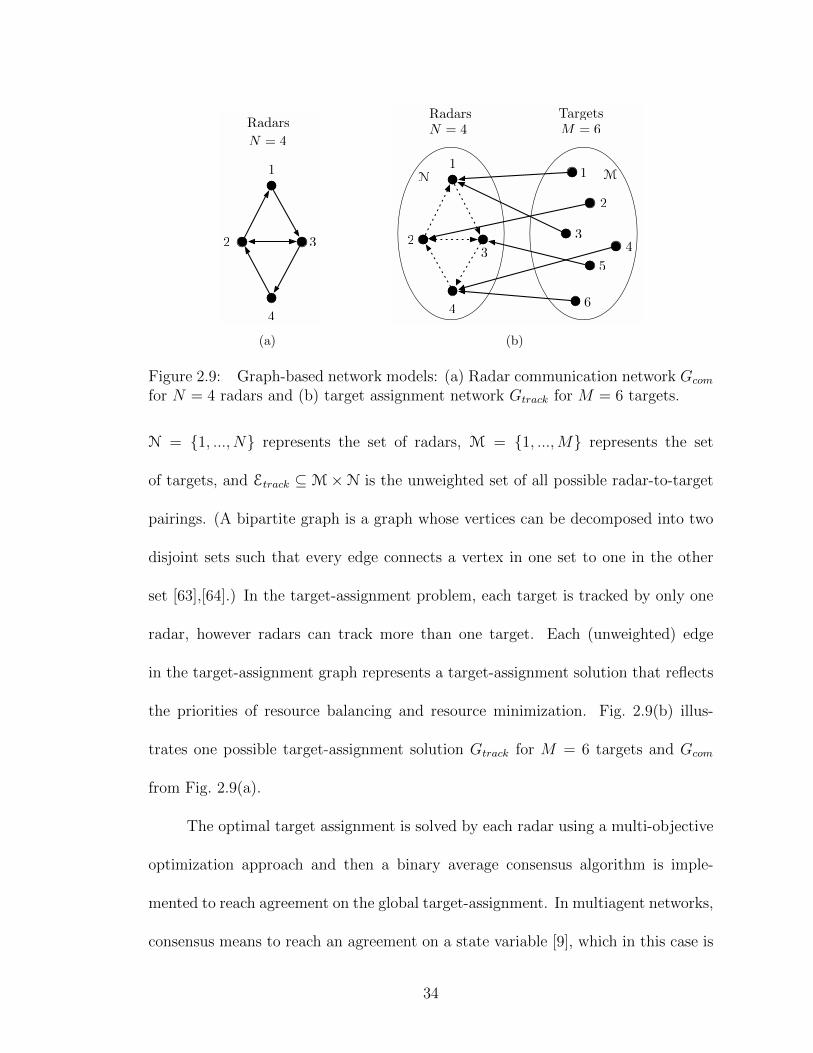
Figure 2.9: Graph-based network models: (a) Radar communication network Gcom

for N = 4 radars and (b) target assignment network Gtrack for M = 6 targets.

N = 1, ..., N represents the set of radars, M = 1, ...,M represents the set

of targets, and Etrack ⊆M×N is the unweighted set of all possible radar-to-target

pairings. (A bipartite graph is a graph whose vertices can be decomposed into two

disjoint sets such that every edge connects a vertex in one set to one in the other

set [63],[64].) In the target-assignment problem, each target is tracked by only one

radar, however radars can track more than one target. Each (unweighted) edge

in the target-assignment graph represents a target-assignment solution that reflects

the priorities of resource balancing and resource minimization. Fig. 2.9(b) illus-

trates one possible target-assignment solution Gtrack for M = 6 targets and Gcom

from Fig. 2.9(a).

The optimal target assignment is solved by each radar using a multi-objective

optimization approach and then a binary average consensus algorithm is imple-

mented to reach agreement on the global target-assignment. In multiagent networks,

consensus means to reach an agreement on a state variable [9], which in this case is

34

the binary matrix of radar-to-target assignments. A consensus algorithm specifies

the interactions and information exchanges between each radar and all of its neigh-

bors on a network [9]. By using a theoretically justified consensus algorithm [9], the

initial target-assignment solution identified by each radar will be updated in such

a way so as to reach an agreement on a single solution. Consensus algorithms are

guaranteed to converge even under very mild assumptions on the communication

network [10]; indeed, they are tolerant to time-varying, directed communication

links [11] and time-delayed communication [12]. Information can be exchanged ei-

ther synchronously (radars communicate at the same time using a global clock)

or asynchronously (radars take turns communicating without the global clock re-

quirement). An agreement problem in which the agents reach agreement on the

average value of their initial states is called an average-consensus problem [65]. Let

x(n) ∈ RN represent the states of N nodes at time step n, where N = 1, ..., N,

and supposed each node evolves according to the discrete-time [9] dynamics (with

step-size T > 0)

xk(n+ 1) = xk(n) + Tuk. (2.33)

Let Nk represent the set of all nodes j in the neighborhood of node k (i.e., each

node j sends its state information to node k). Olfati-Saber and Murray show [9]

that the linear consensus protocol uk =∑

j∈Nk(xj−xk) solves the average Euclidean

consensus problem for agents communicating over a balanced and strongly connected

digraph. The dynamics of all nodes can be expressed in terms of the graph Laplacian

35

L [9]. Let ε ∈ (0, 1/maxklkk) where k ∈ 1, ..., N. Then

x(n+ 1) = (I − εL)x(n). (2.34)

Cai and Ishii [65] have extended the average-consensus convergence results in 2.34

to consider strongly connected digraphs that are not balanced and present [66]

an average-consensus approach for quantized (integer-valued) information flow on

asynchronous networks.

36

Chapter 3

Distributed Optimization and Validation in Two Dimensions

This chapter presents a dynamic load balancing approach to resource alloca-

tion for optimizing the search and track performance of multiple shipboard radars. A

2D linear radar model is introduced in Section 3.2 that is an idealized version of the

3D nonlinear radar model presented in Section 2.2.1. Using the linear model, Sec-

tion 3.2.1 provides theoretically justified strategies to maximize the collective search

area for up to three radars by solving for each radar’s optimal location, search-area

radius, and search sector. Section 3.2.2 solves for the optimal target-assignment

by balancing the search and track tasking among coordinated radars, increasing

the number of trackable targets, and show that the assignment boundaries are hy-

perbolic. Section 3.3 extends the search area maximization and target-assignment

optimization approaches from Sections 3.2.1 and Section 3.2.2 to a nonlinear 2D

radar model.

3.1 Optimization Approach

To solve the target-assignment problem, each radar seeks the target-assignment

solution for the entire network that balances radar resource usage across the radar

network. Radar resource usage depends on the search and track requirements. Bal-

ancing the resource utilization among coordinated radars prevents a single radar

37

from using all of its available resources, unless the other radars are also at their

maximum capacity, which is important if a majority of the targets are detected by

a subset of sensors. Coordinated radars can track targets in another radar’s search

area; an uncoordinated radar can only track targets within its own search area.

3.2 Linear Radar Model

Recall in a multifunction radar system that the radar performs two primary

tasks, search and track [38]. During search, the radar sends out a focused search

beam covering a subset of the search sector and looks for a target. If no target is

detected, then the search beam moves to the next location until the entire sector

is searched. If a target is detected, the radar tracks it by periodically sampling

the projected target location. In a variable resource doctrine, if resources are fully

consumed by tracking targets, the radar will suspend searching for new targets until

resources are freed from tracking requirements. The operating environment is the

set of all possible shipboard radar positions (x, y) ∈ R2 and target locations. The

distance between radar j and radar k is denoted δj,k =√

(xj − xk)2 + (yj − yk)2.

Assume that radar k performs uniform surveillance tasks that consume radar

resources as a linear function of both the search coverage sector Ωk and detection

range ρk. The detection range is equal to the radius of the search sector and satisfies

the requirements of the maximum unambiguous range 2.2. Tracking tasks consume

resources as a linear function of the range ρm,k to the target and number of targets

in track (see Fig. 3.1). A resource reserve εk is also specified, where 0 ≤ εk ≤ 1,

38

which represents the fraction of the total (unit) resource that cannot be used for

search or track. Each radar communicates over the radar network Gcom as described

in Section 2.3.2.

For M ≥ 2 targets, a second network, Gtrack = (M, N , Et), called the

target-assignment network is considered as discussed in Section 2.3.3. The target

assignment problem is to optimize Gtrack given the radar network Gcom. (In the case

of M = 1 target, the target assignment problem is to solve for the optimal radar-

to-target assignment.) Linear models for resource consumption for search, Tsearch,k

and Ttrack,k, by radar k ∈ 1, . . . , N are

Tsearch,k = a(ρk + Ωk) and (3.1)

T(tot)track,k = c

Mk∑m=1

ρm,k, (3.2)

where a, c ∈ R+ are radar parameters common to each (identical) radar and each

radar searches a single sector. Each radar consumes resources to meet its search

requirements, but when radars coordinate on target assignment, only the radar

assigned to track the target of interest consumes resources for tracking. Since Tmax

is the maximum resource availability of each radar k, the total resource consumed

by radar k is

Pk = (Tsearch,k + T(tot)track,k + εk)/Tmax, (3.3)

with resource reserve constraint

Pk ≤ 1. (3.4)

39

targets

ship

Ωi

ρi

3

i

ρ1,k

ρ 2,k

ρ 3,i

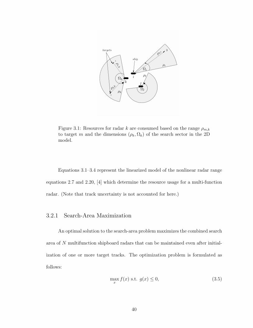
Figure 3.1: Resources for radar k are consumed based on the range ρm,kto target m and the dimensions (ρk,Ωk) of the search sector in the 2Dmodel.

Equations 3.1–3.4 represent the linearized model of the nonlinear radar range

equations 2.7 and 2.20, [4] which determine the resource usage for a multi-function

radar. (Note that track uncertainty is not accounted for here.)

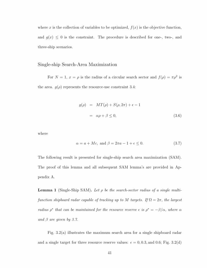
3.2.1 Search-Area Maximization

An optimal solution to the search-area problem maximizes the combined search

area of N multifunction shipboard radars that can be maintained even after initial-

ization of one or more target tracks. The optimization problem is formulated as

follows:

maxx

f(x) s.t. g(x) ≤ 0, (3.5)

40

where x is the collection of variables to be optimized, f(x) is the objective function,

and g(x) ≤ 0 is the constraint. The procedure is described for one-, two-, and

three-ship scenarios.

Single-ship Search-Area Maximization

For N = 1, x = ρ is the radius of a circular search sector and f(ρ) = πρ2 is

the area. g(ρ) represents the resource-use constraint 3.4:

g(ρ) = MT (ρ) + S(ρ, 2π) + ε− 1

= αρ+ β ≤ 0, (3.6)

where

α = a+Mc, and β = 2πa− 1 + ε ≤ 0. (3.7)

The following result is presented for single-ship search area maximization (SAM).

The proof of this lemma and all subsequent SAM lemma’s are provided in Ap-

pendix A.

Lemma 1 (Single-Ship SAM). Let ρ be the search-sector radius of a single multi-

function shipboard radar capable of tracking up to M targets. If Ω = 2π, the largest

radius ρ∗ that can be maintained for the resource reserve ε is ρ∗ = −β/α, where α

and β are given by 3.7.

Fig. 3.2(a) illustrates the maximum search area for a single shipboard radar

and a single target for three resource reserve values: ε = 0, 0.3, and 0.6; Fig. 3.2(d)

41

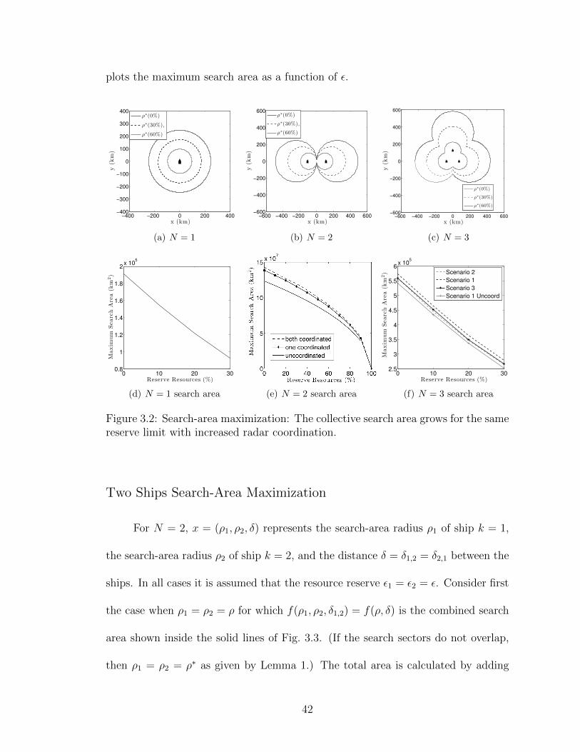
plots the maximum search area as a function of ε.

−400 −200 0 200 400−400

−300

−200

−100

0

100

200

300

400

x (km)

y(k

m)

ρ∗(0%)

ρ∗(30%),

ρ∗(60%)

(a) N = 1

−600 −400 −200 0 200 400 600−600

−400

−200

0

200

400

600

x (km)

y(k

m)

ρ∗(0%)

ρ∗(30%),

ρ∗(60%)

(b) N = 2

−600 −400 −200 0 200 400 600−600

−400

−200

0

200

400

600

x (km)

y(k

m)

ρ∗(0%)

ρ∗(30%)

ρ∗(60%)

(c) N = 3

0 10 20 300.8

1

1.2

1.4

1.6

1.8

2x 10

5

Reserve Resources (%)

Maxim

um

Searc

hA

rea

(km

2)

(d) N = 1 search area (e) N = 2 search area

0 10 20 302.5

3

3.5

4

4.5

5

5.5

6x 10

5

Reserve Resources (%)M

axim

um

Searc

hA

rea

(km

2)

Scenario 2

Scenario 1

Scenario 3

Scenario 1 Uncoord

(f) N = 3 search area

Figure 3.2: Search-area maximization: The collective search area grows for the samereserve limit with increased radar coordination.

Two Ships Search-Area Maximization

For N = 2, x = (ρ1, ρ2, δ) represents the search-area radius ρ1 of ship k = 1,

the search-area radius ρ2 of ship k = 2, and the distance δ = δ1,2 = δ2,1 between the

ships. In all cases it is assumed that the resource reserve ε1 = ε2 = ε. Consider first

the case when ρ1 = ρ2 = ρ for which f(ρ1, ρ2, δ1,2) = f(ρ, δ) is the combined search

area shown inside the solid lines of Fig. 3.3. (If the search sectors do not overlap,

then ρ1 = ρ2 = ρ∗ as given by Lemma 1.) The total area is calculated by adding

42

the individual search areas and subtracting the area of overlap. The area of overlap

is found by calculating the area of each sector described by θ1,2 = θ2,1 = θ (use

Fig. 3.3 and subtract the area of the triangles 1AB and 2AB). Using the identity

cosu sin v = 1/2(sin(u+ v) + sin(u− v)), the total area is

f(ρ, δ) = 2πρ2 − 2

(θ

2ππρ2)

+ 4

(1

2ρ cos

θ

2ρ sin

θ

2

)= (2π − θ + sin θ)ρ2. (3.8)

An expression for θ in terms of δ and ρ is found by solving cos(θ/2) = δ/(2ρ)

for θ. Since 1− δ/(2ρ) > 0 in order for the sensor areas to overlap, this implies that

δ/(2ρ) < 1 and therefore 0 < cos(θ/2) < 1, which implies 0 < θ < π. Note that

sin θ − θ ≤ 0 decreases as θ ≥ 0 increases. Thus the total search area is maximized

when sin θ − θ is maximized, which corresponds to smaller values of θ. Performing

a Taylor series expansion of cos(θ/2) about θ/2 = 0 yields

δ

2ρ= cos

(θ

2

)= 1− θ2

8+ H.O.T. (3.9)

The higher order terms in 3.9 are dropped since including them further in the

analysis does not significantly affect the values for the overlap angle θ. Solving

for θ yields

θ ≈ 2

√2− δ

ρ. (3.10)

In the two-ship scenario with overlapping search areas, the area of overlap

43

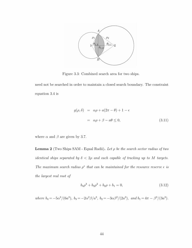
ρ1 ρ2

θ1,2 θ2,1

δ1,2

Figure 3.3: Combined search area for two ships.

need not be searched in order to maintain a closed search boundary. The constraint

equation 3.4 is

g(ρ, δ) = αρ+ a(2π − θ) + 1− ε

= αρ+ β − aθ ≤ 0, (3.11)

where α and β are given by 3.7.

Lemma 2 (Two Ships SAM - Equal Radii). Let ρ be the search sector radius of two

identical ships separated by δ < 2ρ and each capable of tracking up to M targets.

The maximum search radius ρ∗ that can be maintained for the resource reserve ε is

the largest real root of

b4ρ3 + b3ρ

2 + b2ρ+ b1 = 0, (3.12)

where b4 =−5α3/(6a3), b3 =−2α2β/a3, b2 =−3αβ2/(2a3), and b1 = 4π − β3/(3a3).

44

The optimal ship separation is

δ∗ ≈ ρ∗

(2−

(αρ∗ + β

2a

)2). (3.13)

Each radar’s search radius is solved using 3.12 and position using 3.13. Fig. 3.2(b)

illustrates the results of the N = 2, M = 1 search-area maximization for the same

three reserve values.

As shown in Table 3.1, consideration is given to the N = 2 case where the

optimal search radius of each shipboard radar is sought given their position. Note

that the spacing δ must still satisfy δ < ρ1 + ρ2.

Lemma 3 (Two Ships SAM - Equal Radii - Given Position). Given N = 2 ships with

ρ1 = ρ2 = ρ and θ1,2 = θ2,1 that are separated by the distance δ1,2 = δ, the maximum

search radius that can be maintained for the resource reserve ε is the largest real root

of 3.12, where b4 = α2/(4a2), b3 = 2αβ/(4a2), b2 = β2/(4a2)− 2, and b1 = δ.

Consider next a scenario in which neither the search radii ρ1 and ρ2 nor the

overlapping search angles θ1,2 and θ2,1 are equal. One example occurs when ρ1 = ρ∗

(the N = 1 optimal radius), and ρ2 and δ are optimized to maximize the com-

bined search area. This scenario demonstrates the interoperability of the proposed

algorithm with pre-existing uncoordinated radar tasking. The objective function

f(ρ1, ρ2, δ) is the combined search area and x = (ρ1, ρ2, δ) = (ρ∗, ρ2, δ). The com-

bined search area is

f(ρ∗, ρ2, δ)=ρ∗2

2(2π − θ1,2 + sin θ1,2) +

ρ222

(2π − θ2,1 + sin θ2,1), (3.14)

45

where

θ1,2 = 2 arccos

(δ2 + ρ∗2 − ρ22

2δρ∗

)(3.15)

and

θ2,1 = 2 arccos

(δ2 − ρ∗2 + ρ22

2δρ2

). (3.16)

The objective function is maximized when both θ1,2 and θ2,1 are small and the

overlap angles are expressed in terms of δ and ρ2 using Taylor series expansions:

δ2 + ρ∗2 − ρ222δρ∗

≈ cos

(θ1,22

)= 1−

θ21,28

(3.17)

δ2 − ρ∗2 + ρ222δρ2

≈ cos

(θ2,12

)= 1−

θ22,18. (3.18)

Solving for θ1,2 and θ2,1 yields

θ1,2 ≈ 2

√2

(1− δ2 + ρ∗2 − ρ22

2δρ∗

)(3.19)

θ2,1 ≈ 2

√2

(1− δ2 − ρ∗2 + ρ22

2δρ2

). (3.20)

The distance δ between the two ships as a function of the search radius ρ2 and

search angle θ2,1 is found by solving 3.20 for δ:

δ2 + δ

(ρ2θ

22,1

4− 2ρ2

)+ ρ22 − ρ∗

2 ≈ 0. (3.21)

46

Table 3.1: Availability of Search-Area Maximization Analytical Results for N = 2and N = 3 ships (? indicates numerical solution, X indicates analytical solutionpresented in this chapter.)

Radius given Position Radius and PositionEq Rad Two Eq Rad Uneq Rad Eq Rad Two Eq Rad Uneq Rad

N = 2 Lem 3 – Lem 4 Lem 2 – XScen 1 Lem 6 Lem 7 Lem 7 Lem 5 X XScen 2 Lem 9 ? ? Lem 8 ? ?Scen 3 ? ? ? ? ? ?

Solving 3.11 with ρ replaced by ρ2 and θ replaced by θ2,1 yields

θ2,1 =αρ2 + β

b. (3.22)

Substituting 3.22 into 3.21, noting that ρ2 ≥ ρ∗, yields two positive real roots with

one root less than one and the other greater than one. The larger root is chosen in

order to maximize 3.14, which yields

δ =4

8a2

√b6ρ82 + b5ρ72 + b4ρ62 + b3ρ52 + b2ρ42 + b1ρ32 + 4a4ρ∗2

− 1

8a2(α2ρ42 + 2αβρ32 + β2ρ22 − 8a2ρ2

), (3.23)

where b6 =α4/16, b5 =βα3/4, b4 =3β2α2, b3 =(β3α/4−α2a2), b2 =(β4/16−2βαa2),

and b1 =−β2a2.

Using sin θ1,2 ≈ θ1,2 and sin θ2,1 ≈ θ2,1 in 3.14 yields

f(ρ∗, ρ2, δ) ≈ πρ∗2 −θ31,2ρ

∗2

12+ πρ22 −

θ32,1ρ22

12. (3.24)

47

Taking the derivative of 3.24 with respect to ρ2 gives

∂f

∂ρ2= −1

4ρ∗2θ21,2

∂θ1,2∂ρ2

+ 2πρ2 −1

6θ32,1ρ2 −

1

4ρ22θ

22,1

∂θ2,1∂ρ2

, (3.25)

where θ2,1 is given by 3.22 with ∂θ2,1/∂ρ2 = α/a, and θ1,2 is given in 3.19. Evaluating

∂f/∂ρ2 = 0 yields the optimal search radius ρ∗2, and the results in 3.25 can be used

to solve for the optimal spacing δ∗.

The N = 2 search area maximization analysis are concluded by considering a

scenario in which the search radii ρ1 and ρ2 are not equal and the goal is to find the

optimal search-sector radius of each ship given their position.

Lemma 4 (Two Ships SAM - Unequal Radii - Given Position). Given two ships

separated by distance δ1,2 < ρ1 + ρ2, with ρ1 = ρ∗ (the N = 1 optimal radius),

ρ1 6= ρ2, and θ1,2 6= θ2,1, the maximum search radius ρ2∗ that can be maintained for

the resource reserve ε is the largest real root of

b4ρ32 + b3ρ

22 + b2ρ

22 + b1 = 0, (3.26)

where b4 = δα2/(4a2), b3 = 2δαβ/(4a2) + 1, b2 = δβ2/(4a2)− 2δ, and b1 = δ2 + ρ∗2.

Fig. 3.2(e) compares the N = 2 maximum search areas for the following three

scenarios: (1) both ships coordinating on the combined search area and ρ1 = ρ2 = ρ∗

from Lemma 2; (2) ship k = 2 coordinating on the combined search area and

ship k = 1 searching with a radius ρ1 = ρ∗ from Lemma 1; and (3) neither ship

coordinating on the combined search area, i.e., ρ1 = ρ2 = ρ∗ from Lemma 1 and δ is

48

chosen such that δ < 2ρ∗. Note that the combined search area is greater when both

ships coordinate the optimization of their search radii and spacing.

Three or More Ships Search-Area Maximization

Consider three or more shipboard multifunction radars that are tasked to

protect a prioritized list of defended assets and/or search specific launch areas for

targets. Because it is unlikely for N > 3 shipboard radars to have overlapping search

areas due to the large spacing between the target launch locations as compared to the

radar search area, solving the N = 1, 2, and 3 search-area maximization problems

suggests a solution for an arbitrary number of ships. The N = 3 analysis seeks

to maximize the combined search area f(x), subject to the reserve constraint g(x),

where x = (ρ1, ρ2, ρ3, δ1,2, δ1,3, δ2,3) and ε1 = ε2 = ε3 = ε. Note f(x) is the total area

searched by all three radars less any overlap between radars.

Three possible scenarios are considered for N = 3 shipboard multifunction

radars, depending on the desired search mission (see Fig. 3.4). Scenario 1 occurs

when a single ship’s search area overlaps two other ship’s search areas but the other

two ships do not overlap with each other. Scenario 2 occurs when all three ships

have a pairwise search-area overlap with each other but no common overlap area for

all three ships. Scenario 3 occurs when all three ships have a common search overlap

area. In this scenario, the area of common overlap is called a circular triangle [67].

The combined search area for any of the three N = 3 scenarios is calculated

by adding the individual search areas and subtracting the total area of overlap. The

49

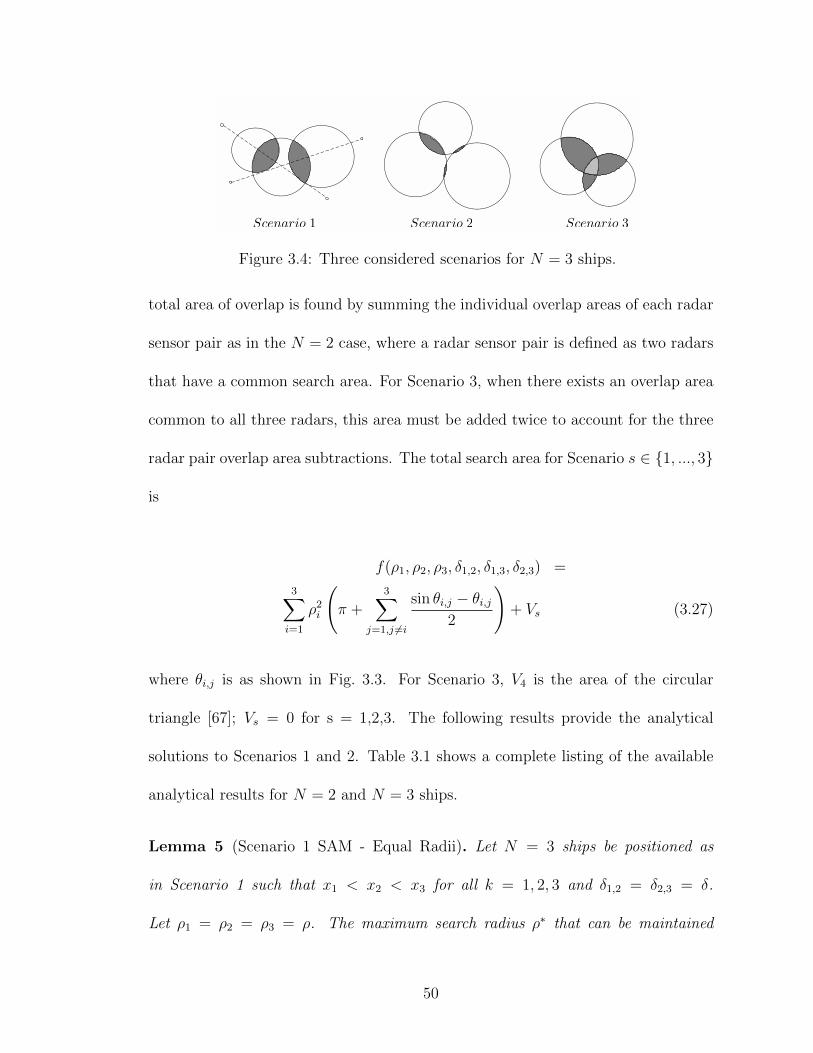
Figure 3.4: Three considered scenarios for N = 3 ships.

total area of overlap is found by summing the individual overlap areas of each radar

sensor pair as in the N = 2 case, where a radar sensor pair is defined as two radars

that have a common search area. For Scenario 3, when there exists an overlap area

common to all three radars, this area must be added twice to account for the three

radar pair overlap area subtractions. The total search area for Scenario s ∈ 1, ..., 3

is

f(ρ1, ρ2, ρ3, δ1,2, δ1,3, δ2,3) =

3∑i=1

ρ2i

(π +

3∑j=1,j 6=i

sin θi,j − θi,j2

)+ Vs (3.27)

where θi,j is as shown in Fig. 3.3. For Scenario 3, V4 is the area of the circular

triangle [67]; Vs = 0 for s = 1,2,3. The following results provide the analytical

solutions to Scenarios 1 and 2. Table 3.1 shows a complete listing of the available

analytical results for N = 2 and N = 3 ships.

Lemma 5 (Scenario 1 SAM - Equal Radii). Let N = 3 ships be positioned as

in Scenario 1 such that x1 < x2 < x3 for all k = 1, 2, 3 and δ1,2 = δ2,3 = δ.

Let ρ1 = ρ2 = ρ3 = ρ. The maximum search radius ρ∗ that can be maintained

50

for the resource reserve ε is the largest root of 3.12, where b4 = −5α3/(3a3), b3 =

−4α2β/a3, b2 =(−3αβ2)/a3, and b1 =6π − 2β3/(3a3). The optimal ship separation

δ∗ is given by 3.13.

Lemma 6 (Scenario 1 SAM - Equal Radii - Given Position). Let N = 3 ships in

Scenario 1 be positioned as in Lemma 5 with ρ1 = ρ2 = ρ3 = ρ and δ1,2 = δ2,3 =

δ. The maximum radar search radius ρ∗ that can be maintained for the resource

reserve ε is the largest real root of 3.12, where b4 = α2/(4a2), b3 = 2αβ/(4a2), b2 =

β2/(4a2)− 2, and b1 = δ.

To satisfy the optimality condition g(ρ∗, δ) = 0, each ship position must sat-

isfy 3.13 for at least one real root ρ∗. Choosing δ ≤ 2ρ1 where ρ1 is the optimal

radius ρ∗ from N = 1 ensures a solution to 3.13.

Lemma 7 (Scenario 1 SAM - Unequal Radii). Let N = 3 ships in Scenario 1 be

positioned as in Lemma 5 with at least two radars having unequal radii and the

radius ρ2 is prescribed. The maximum search radii ρ1 and ρ3 are both equal to the

largest real root of 3.26.

Consider next Scenario 1 with N = 3 ships positioned as in Lemma 5 with

at least two radars having unequal radii. Let ρ2 = ρ∗ from Lemma 1 and δ1,2 =

δ2,3 = δ. The objective function f(ρ1, ρ2, ρ3, δ) is the combined search area and

x = (ρ1, ρ2, ρ3, δ) = (ρ1, ρ∗, ρ3, δ). The combined search area is given in 3.27 with

θ1,2, θ2,1, θ2,3, and θ3,2 given in A.11–A.14 respectively. The combined search area is

maximized when the overlap angle for each ship pair, θj,k, is small, thus a Taylor

series expansion of sin θj,k is performed about θj,k = 0 in 3.27 to obtain A.16. (In

51

what follows, the procedure for solving for search radii ρ1 and ρ3 are identical, thus

only ρ1 is described.)

The distance δ1,2 as a function of the search radius ρ1 and search angle θ1,2 is

found by solving 3.19 for δ to yield

δ2 + δ

(ρ∗2θ21,2

4− 2ρ∗

)+ ρ∗2 − ρ12 ≈ 0. (3.28)

Solving 3.11 with ρ replaced by ρ1 and θ replaced by θ1,2 yields

θ1,2 =αρ1 + β

b(3.29)

Substituting 3.29 into 3.28, noting that ρ1 ≥ ρ∗, yields two positive real roots with

one root less than one and the other greater than one. The larger root is chosen

in order to maximize 3.27, which yields 3.23 with ρ2 replaced by ρ1. Taking the

derivative of A.16 with respect to ρ1 gives

∂f

∂ρ1= 2πρ1 −

1

6θ31,2ρ1 −

1

4ρ1

2θ21,2∂θ1,2∂ρ1

− 1

4ρ∗2θ22,1

∂θ2,1∂ρ1

, (3.30)

where θ1,2 is given by 3.22 with ∂θ1,2/∂ρ1 = α/a, and θ2,1 is given by A.12. Evalu-

ating ∂f/∂ρ1 = 0 yields the optimal search radius ρ∗1, and the results in 3.30 can be

used to solve for the optimal spacing δ∗.

Lemma 8 (Scenario 2 SAM - Equal Radii - Given Position). Let N = 3 sensors be

positioned as in Scenario 2 such that x1 < x2, x2 < x3, y1 > y2, and y2 < y3. Let

52

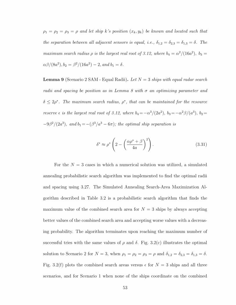
ρ1 = ρ2 = ρ3 = ρ and let ship k’s position (xk, yk) be known and located such that

the separation between all adjacent sensors is equal, i.e., δ1,2 = δ2,3 = δ1,3 = δ. The

maximum search radius ρ is the largest real root of 3.12, where b4 = α2/(16a2), b3 =

αβ/(8a2), b2 = β2/(16a2)− 2, and b1 = δ.

Lemma 9 (Scenario 2 SAM - Equal Radii). Let N = 3 ships with equal radar search

radii and spacing be position as in Lemma 8 with σ an optimizing parameter and

δ ≤ 2ρ∗. The maximum search radius, ρ∗, that can be maintained for the resource

reserve ε is the largest real root of 3.12, where b4 =−α3/(2a2), b3 =−α2β/(a3), b2 =

−9β2/(2a3), and b1 =−(β3/a3 − 6π); the optimal ship separation is

δ∗ ≈ ρ∗

(2−

(αρ∗ + β

4a

)2). (3.31)

For the N = 3 cases in which a numerical solution was utilized, a simulated

annealing probabilistic search algorithm was implemented to find the optimal radii

and spacing using 3.27. The Simulated Annealing Search-Area Maximization Al-

gorithm described in Table 3.2 is a probabilistic search algorithm that finds the

maximum value of the combined search area for N = 3 ships by always accepting

better values of the combined search area and accepting worse values with a decreas-

ing probability. The algorithm terminates upon reaching the maximum number of

successful tries with the same values of ρ and δ. Fig. 3.2(c) illustrates the optimal

solution to Scenario 2 for N = 3, when ρ1 = ρ2 = ρ3 = ρ and δ1,2 = δ2,3 = δ1,3 = δ.

Fig. 3.2(f) plots the combined search areas versus ε for N = 3 ships and all three

scenarios, and for Scenario 1 when none of the ships coordinate on the combined

53

Table 3.2: Simulated Annealing Search-Area Maximization Algorithm [47]

Input: Perturb function to update the input values X, h(X) : Rn → Rn,

cost function J : Rn → R to compare candidate solutions,

constraint function G : Rn → R, and a non-increasing cooling

schedule T(n+ 1) = kT (n),where 0 < k < 1.

Initialize: Estimate at current time step, X(1).

Complete the following steps for n = 1, 2, 3... until a termination criteria is reached.

1. Generate X ′(n) = h(X(n)) and calculate J(X(n)) and J(X ′(n))

2. Set J(X ′(n)) = 0 if G(X ′(n)) > 0. (constraint violated)

3. Sample from a uniform distribution r ∼ U(0, 1) and update X according to:

X(n+ 1) =

X ′(n) if r < exp(−(J(X(n))−J(X′(n)))

kT (n)

)X(n) otherwise

where T (n) is the current temperature.

4. Update the temperature based on the cooling schedule.

search area.

3.2.2 Target Assignment Optimization

This section poses and solves an optimal target-assignment problem that seeks

to balance the search and track tasking between multi-function radar systems. It

starts by considering M = 1 target for N = 3 shipboard multifunction radars and

shows that the solution to the target-assignment problem has a hyperbolic bound-

ary determined by the search-area radii and distance to the target. The results are

extended to M > 1 targets and the target assignment boundary for target M is

solved for, assuming targets 1, ...,M − 1 are already being tracked. In each case

it is assumed that all N = 3 ships have exact knowledge of the position of targets

54

1, ...,M . A combination of analytical and numerical solutions are presented to high-

light the results.

Prior knowledge of the hyperbolic “switching” boundary for multi-function

radars has many benefits. For example, target handovers or migrations can nega-

tively affect the accuracy of the target state information during the time it takes

the new tracking radar to search for and acquire the target, even with accurate

information from the previous tracker. Knowledge of the target-switching bound-

ary also allows a radar to be prepared to track a new target, in effect the radar is

cued beforehand and can plan tasking accordingly. Another benefit of knowing the

target-assignment boundary is the ability to optimize the ship and radar placement

relative to the target(s). Finally, in the event that a target is or will be soon engaged,

the target-switching boundary allows for radars to anticipate a handover that may

occur during or just prior to an engagement order and thus delay or prevent the

target from switching from one radar to another avoid any loss or degradation in

the target state information.

Four possible cases of radar performance are considered to evaluate the target-

assignment algorithm. Case (i) – Unoptimized/Uncoordinated occurs when the

radars do not optimize their combined search area and do not coordinate on the

target assignment. Case (ii) – Unoptimized/Coordinated occurs when the radars

do not optimize their combined search area but coordinate on the target assign-

ment. This case could arise when the radar locations are fixed or when the radar

ship platforms must remain in a particular location for other operational mission

requirements. Case (iii) – Optimized/Uncoordinated occurs when the combined

55

search area is optimized but the radars do not coordinate on the target assignment.

This case could arise if the ship positions and radar search radii were remotely

optimized prior to arriving on station. Case (iv) – Optimized/Coordinated occurs

when the combined search area is optimized and the radars coordinate on the target

assignment.

Single Target Assignment

Recall the total resource loading Pk of ship k defined in 3.3. A balanced radar

resource loading between all pairs of communicating radars can be accomplished by

minimizing the absolute value of the difference |Pk−Pl| between their loading for all

connected pairs k, l, consistent with the resource reserves εk, εl. By minimizing the

difference between the total resource loading between each shipboard radar pair, a

balanced radar resource loading among all radars is achieved. A balanced approach

is shown here to increase the trackable area and allow more targets to be tracked

within a given search area.

Let M = 1 and j be the index of the tracking ship. The measure of resource

balancing among all ships is

Cj(Gcom) =∑

(k,l)∈Es

(Pk − Pl)2 , (3.32)

56

where Gcom is the (undirected) ship communication network. The optimal target

assignment for Gcom that balances the radar tasking between all pairs of ships is

j∗ = argminj∈1,...,N

Cj(Gcom). (3.33)

The optimal target assignment for N = 3 ships and M = 1 target is compute-

dusing the target-assignment optimization algorithm in Table 3.3. Note that the set

of possible target positions assigned to a ship is called the track zone. Fig. 3.5(a) il-

lustrates the solution to the target-assignment problem for Cases (i)–(iv) introduced

earlier. Note that in Case (ii) (three ships whose search area is not optimized but

coordinate on target assignment) ship k = 1 and ship k = 3 are assigned tracking

responsibilities inside ship k = 2’s search area. Also note that in Case (iii) (three

ships whose search area is optimized but are not coordinated on target assignment)

all ships track target M = 1 in their respective search overlap areas, thus expending

twice as many resources as necessary.

Fig. 3.5(b) compares the radar tasking of all four cases and verifies that the optimal

target assignment balances radar tasking. In the cases where the search area and

ship positions are optimized, the optimal solution also yields an increase in the

trackable area.

For Cases (ii) and (iv) (all three ships coordinate their target assignment), the

solution to the target assignment problem for any pair of ships is a conic section

that describes the boundary between the track zones. In Case (ii) the solution is a

pair of hyperbolic boundaries, whereas in Case (iv) the solution is a line.

57

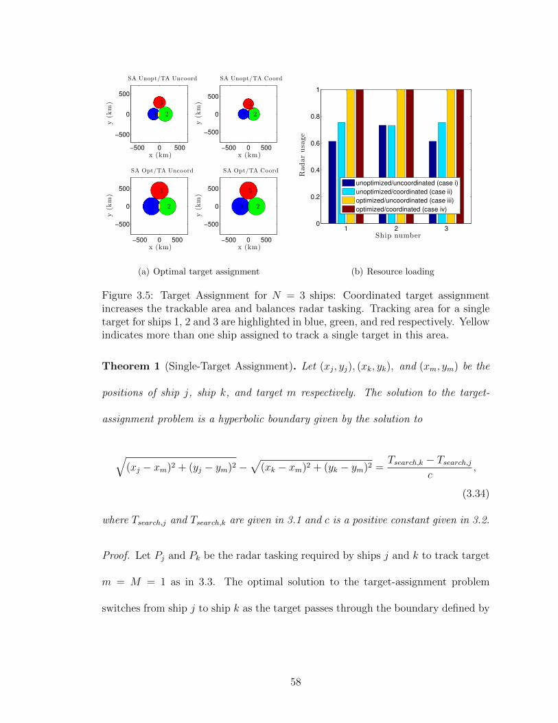
x (km)

y(k

m)

SA Unopt/TA Uncoord

1 2

3

−500 0 500

−500

0

500

x (km)

y(k

m)

SA Unopt/TA Coord

1 2

3

−500 0 500

−500

0

500

x (km)

y(k

m)

SA Opt/TA Uncoord

1 2

3

−500 0 500

−500

0

500

x (km)

y(k

m)

SA Opt/TA Coord

1 2

3

−500 0 500

−500

0

500

(a) Optimal target assignment

1 2 30

0.2

0.4

0.6

0.8

1

Ship number

Radar

usa

ge

unoptimized/uncoordinated (case i)

unoptimized/coordinated (case ii)

optimized/uncoordinated (case iii)

optimized/coordinated (case iv)

(b) Resource loading

Figure 3.5: Target Assignment for N = 3 ships: Coordinated target assignmentincreases the trackable area and balances radar tasking. Tracking area for a singletarget for ships 1, 2 and 3 are highlighted in blue, green, and red respectively. Yellowindicates more than one ship assigned to track a single target in this area.

Theorem 1 (Single-Target Assignment). Let (xj, yj), (xk, yk), and (xm, ym) be the

positions of ship j, ship k, and target m respectively. The solution to the target-

assignment problem is a hyperbolic boundary given by the solution to

√(xj − xm)2 + (yj − ym)2 −

√(xk − xm)2 + (yk − ym)2 =

Tsearch,k − Tsearch,jc

,

(3.34)

where Tsearch,j and Tsearch,k are given in 3.1 and c is a positive constant given in 3.2.

Proof. Let Pj and Pk be the radar tasking required by ships j and k to track target

m = M = 1 as in 3.3. The optimal solution to the target-assignment problem

switches from ship j to ship k as the target passes through the boundary defined by

58

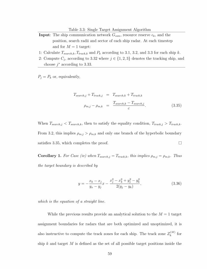
Table 3.3: Single Target Assignment Algorithm

Input: The ship communication network Gcom, resource reserve εk, and the

position, search radii and sector of each ship radar. At each timestep

and for M = 1 target:

1: Calculate Tsearch,k, Ttrack,k and Pk according to 3.1, 3.2, and 3.3 for each ship k.

2: Compute Cj, according to 3.32 where j ∈ 1, 2, 3 denotes the tracking ship, and

choose j∗ according to 3.33.

Pj = Pk or, equivalently,

Tsearch,j + Ttrack,j = Tsearch,k + Ttrack,k

ρm,j − ρm,k =Tsearch,k − Tsearch,j

c. (3.35)

When Tsearch,j < Tsearch,k, then to satisfy the equality condition, Ttrack,j > Ttrack,k.

From 3.2, this implies ρm,j > ρm,k and only one branch of the hyperbolic boundary

satisfies 3.35, which completes the proof.

Corollary 1. For Case (iv) when Tsearch,j = Ttrack,k, this implies ρm,j = ρm,k. Thus

the target boundary is described by

y = −xk − xjyx − yj

x−x2j − x2k + y2j − y2k

2(yj − yk), (3.36)

which is the equation of a straight line.

While the previous results provide an analytical solution to the M = 1 target

assignment boundaries for radars that are both optimized and unoptimized, it is

also instructive to compute the track zones for each ship. The track zone Z(M)k for

ship k and target M is defined as the set of all possible target positions inside the

59

combined search area for ships j = 1, ...,N, where ship j coordinates with ship k

such that the resource loading is most balanced when ship k tracks target M . The

following is a mathematical description of Z(M)k .

Proposition 1 (Single-Target Track Zone). Let (x, y) ∈ R2 be the position of target

M = 1. The track zone Z(M)k for ship k is the set Z

(M)k =

N⋂j=1

Z(M)k,j , where

Z(M)k,j =

(x, y)|

√(xk−x)2+(yk−y)2 ≤ ρk+ρj,k

⋂√

(xj−x)2+(yj−y)2 ≤ ρj⋂

√(xk−x)2+(yk−y)2+aρk+bΩk ≤ (1−ε)

⋂√

(xk−x)2+(yk−y)2 ≤√

(xj−x)2+(yj−y)2+aρj+bΩj−aρk−bΩk

c

.

(3.37)

Fig. 3.6 depicts the analytical solution to the target assignment boundaries

and track zones for Case (ii) when the radars are unoptimized and coordinated.

Multi-Target Assignment

For M > 1 targets, the objective is to balance the radar tasking among all

shipboard radars in the communication network Gcom, where the radar tasking Pk

for ship k now includes the total tracking cost for all Mk targets assigned to ship

k. The measure of the resource balancing among all ships and all targets for a

particular target-assignment network Gtrack and ship communication network Gcom

60

is

C(Gtrack;Gcom) =∑

(k,l)∈Es

(Pk(Gtrack)− Pl(Gtrack))2. (3.38)

Let G∗track = argminGtrackC(Gtrack;Gcom) be the optimal target-assignment network

that balances the radar tasking across ship network Gcom. Then G∗track is computed

using the multi-target assignment algorithm in Table 3.4. For shipboard radars

that coordinate on their target assignment for multiple targets, the following result

is presented.

Theorem 2 (Multi-Target Assignment). For each pair of ships j, k that coordinate

on their target assignment, let m = 1, ...,Mj be the indices of targets tracked

by ship j and l = 1, ...,Mk be the indices of targets tracked by ship k, where

Mj +Mk = M − 1. The target assignment boundary for target M is the solution to

√(xM − xj)2 + (yM − yj)2 −

√(xM − xk)2 + (yM − yk)2 =

Tsearch,k − Tsearch,jc

−Mj∑m=1

√(xm − xj)2 + (ym − yj)2 +

Mk∑l=1

√(xl − xk)2 + (yl − yk)2. (3.39)

Proof. Let T(tot,m)track,j and T

(tot,l)track,k be the total resources consumed by ships j and k

to track targets m and l. The optimal solution to the target assignment problem

for the target M switches from j to k as the target passes through the boundary

Pj,M = Pk,M − T (tot,m)track,j + T

(tot,l)track,k or equivalently

ρM,j − ρM,k =Tsearch,k − Tsearch,j

c−

Mj∑m=1

ρm,j +

Mk∑l=1

ρl,k, (3.40)

61

Table 3.4: Multi-Target Assignment Algorithm

Input: Same as the Single-Target Assignment Algorithm in Table IV.

At each timestep and for each target assignment network Gtrack = (M, Et):

1: Calculate Pk(Gtrack) according to 3.1, 3.2, and 3.3.

2: Calculate C(Gtrack;Gcom) according to 3.38.

3: Find the target assignment network G∗track that minimizes C(Gtrack;Gcom).

which yields 3.39 and completes the proof.

Corollary 2. When Tsearch,k = Tsearch,j, then ρM,k = ρM,j +Mj∑m=1

ρm,j −Mk∑l=1

ρl,k. The

target boundary for target M is the line found by solving

√(xM−xk)2+(yM−yk)2 −

√(xM−xj)2+(yM−yj)2

−Mj∑m=1

√(xj−xm)2+(yj−ym)2 +

Mk∑l=1

√(xl−xk)2+(yl−yk)2 = 0. (3.41)

The multi-target track zone Z(M)k is a function of the positions of the targets

already being tracked by ship k and ship j. For ship k and target M > 1, Z(M)k is

defined as the set of all possible target positions inside the combined search area for

ship j = 1, ...,N, where ship j coordinates with ship k such that the resource loading

is most balanced when ship k tracks target M , assuming Mj is the number of targets

already being tracked by ship j. The following is a mathematical description of the

multi-target track zone.

Proposition 2. Let (x, y) ∈ R2 be the position of target M > 1. The track zone

62

−800−600−400−200 0 200 400 600 800−800

−600

−400

−200

0

200

400

600

800

x (km)

y(k

m)

Ship 1 Track Zone

Ship 2 Track Zone

Ship 3 Track Zone

1

3

2

Figure 3.6: Analytical optimal target assignment boundaries and track zones forM = 1 target.

Z(M)k for ship k is the set Z

(M)k =

N⋂j=1

Z(M)k,j , where

Z(M)k,j =

(x, y)|

√(xk − x)2 + (yk − y)2 ≤ ρk + ρj,k

⋂√

(xj − x)2 + (yj − y)2 ≤ ρj⋂

√(xk − x)2 + (yk − y)2 + aρk + bΩk ≤ (1− ε)

⋂√

(xk − x)2 + (yk − y)2 <√

(xj − x)2 + (yj − y)2 +a(ρj − ρk) + b(Ωj − Ωk)

c

−Mj∑m=1

√(xj − xm)2 + (yj − ym)2 +

Mk∑l=1

√(xk − xl)2 + (yk − yl)2

.

(3.42)

Figs. 3.7(a)–3.7(c) illustrate how the multi-target assignment boundaries and

track zones for the second of two targets changes as the first target passes through

the combined search area of three ships. (The target assignment boundaries and

63

track zones for the first target are shown in Fig. 3.6) The first target is depicted

by a black dot. In Fig. 3.7(a), target M = 1 is being tracked by the leftmost ship

located at (-150,0). In Fig. 3.7(b), target M = 1 is still tracked by the same ship,

however it is approaching the edge of the M = 1 target assignment boundary. In

Fig. 3.7(c), the first target has crossed the M = 1 target assignment boundary and

is now being tracked by the rightmost ship located at (150,0).

3.3 Nonlinear Radar Model

This section presents a Search Area Maximization and Target-Assignment Op-

timization approach using a 2D nonlinear model for radar search and track resource

allocation. The identicalN = 1, 2, and 3 ship scenarios from Sections 3.2.1 and 3.2.2

are considered. Due to the similarity of the approach in this section as compared to

the previous section, the optimization approach is only briefly reviewed; the major-

ity of this subsection focuses on the optimization results, which reinforce the results

of the linear model.

The radar search and track equations given in 3.1 and 3.2 respectively are

modified to account for resource consumption as the fourth power of range. Thus

Tsearch,k = aρ4kΩk , and (3.43)

T(tot)track,k = c

Mk∑m=1

ρ4m,k, (3.44)

64

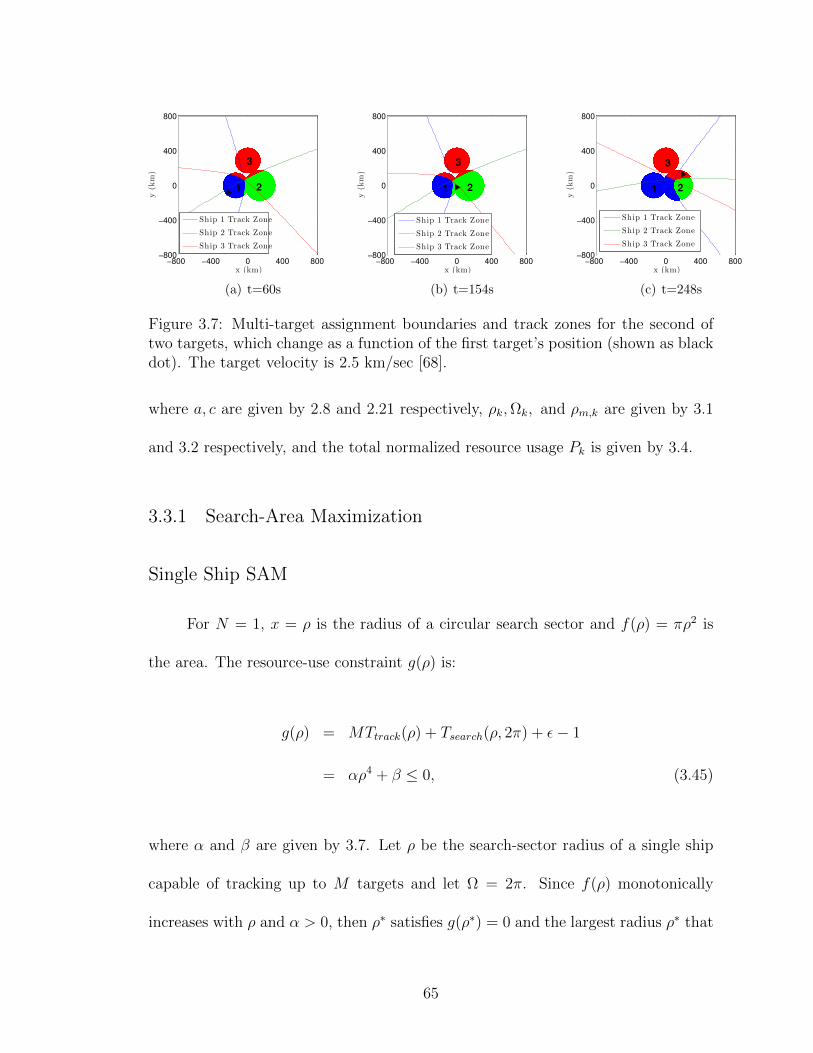
−800 −400 0 400 800−800

−400

0

400

800

x (km)

y(k

m)

Ship 1 Track Zone

Ship 2 Track Zone

Ship 3 Track Zone

3

21

(a) t=60s

−800 −400 0 400 800−800

−400

0

400

800

x (km)

y(k

m)

Ship 1 Track Zone

Ship 2 Track Zone

Ship 3 Track Zone

3

21

(b) t=154s

−800 −400 0 400 800−800

−400

0

400

800

x (km)

y(k

m)

Ship 1 Track Zone

Ship 2 Track Zone

Ship 3 Track Zone

3

21

(c) t=248s

Figure 3.7: Multi-target assignment boundaries and track zones for the second oftwo targets, which change as a function of the first target’s position (shown as blackdot). The target velocity is 2.5 km/sec [68].

where a, c are given by 2.8 and 2.21 respectively, ρk,Ωk, and ρm,k are given by 3.1

and 3.2 respectively, and the total normalized resource usage Pk is given by 3.4.

3.3.1 Search-Area Maximization

Single Ship SAM

For N = 1, x = ρ is the radius of a circular search sector and f(ρ) = πρ2 is

the area. The resource-use constraint g(ρ) is:

g(ρ) = MTtrack(ρ) + Tsearch(ρ, 2π) + ε− 1

= αρ4 + β ≤ 0, (3.45)

where α and β are given by 3.7. Let ρ be the search-sector radius of a single ship

capable of tracking up to M targets and let Ω = 2π. Since f(ρ) monotonically

increases with ρ and α > 0, then ρ∗ satisfies g(ρ∗) = 0 and the largest radius ρ∗ that

65

can be maintained for the resource reserve ε is

ρ∗ = |(−β/α)14 | > 0. (3.46)

Fig. 3.8(a) and 3.8(d) plots the N = 1 results for ε = 0, 0.3, 0.6.

Two- and Three-Ship Search-Area Maximization

The collective search area of N = 2 and N = 3 ships is maximized using

the Simulated Annealing Search-Area Maximization Algorithm in Table 3.2 and the

nonlinear resource constraint

g(ρ, δ) = αρ4 − aθρ4 + β ≤ 0. (3.47)

Figs. 3.8(b); 3.8(e), 3.8(c), and 3.8(f) plot the N = 2 and N = 3 results, respectively.

Note that in both cases, the collective search area is larger if at least one ship is

able to coordinate on the collective search area.

3.3.2 Target Assignment Optimization

Single Target Assignment

To compute the optimal target assignment for N = 3 ships and M = 1 target

for Cases (i)–(iv) described in Section 3.2.2, the single-target assignment algorithm

in Table 3.3 is used. Ship 1 and ship 2 optimize their N = 2 collective search-area

using Table 3.2, whereas ship 3 optimizes its search area using 3.46. Fig. 3.9(a)

66

−400 −200 0 200 400−400

−300

−200

−100

0

100

200

300

400

x (km)

y(k

m)

ρ∗(0%)

ρ∗(30%),

ρ∗(60%)

(a) N = 1

−400 −200 0 200 400−400

−300

−200

−100

0

100

200

300

400

x (km)

y(k

m)

ρ∗(0%)

ρ∗(30%),

ρ∗(60%)

(b) N = 2

−400 −200 0 200 400−400

−300

−200

−100

0

100

200

300

400

x (km)

y(k

m)

(c) N = 3

0 10 20 305.6

5.8

6

6.2

6.4

6.6

6.8

7x 10

7

Reserve Resources (%)

Maxim

um

Sea

rch

Are

a(k

m2)

(d) N = 1 search area

0 20 40 60 80 1000

5

10

15x 10

7

Reserve Resources (%)

Maxim

um

Sea

rch

Are

a(k

m2)

both coordinated

one coordinated

uncoordinated

(e) N = 2 search area

0 20 40 60 80 1000

0.5

1

1.5

2

2.5x 10

8

Reserve Resources (%)

Maxim

um

Sea

rch

Are

a(k

m2)

Scenario 2

Scenario 1

Scenario 3

Scenario 1 Uncoord

(f) N = 3 search area

Figure 3.8: 2D nonlinear search-area maximization: The search area is maximizedwhen at least one shipboard radar is able to coordinate.

illustrates the results. Note that in Case (ii), the track zone for ship 1 extends

into the search area of ship 2. Also observe that in both Case (i) and Case (iii)

(target-assignment uncoordinated), ships 1 and 2 track target M = 1 in their areas

of search overlap (highlighted in yellow), thus expending twice as many resources as

necessary due to redundant tracking. In Case (iv), ships 1 and 2 partition tracking

responsibilities in their collective search area by balancing their resource usage.

Fig. 3.9(b) compares the radar tasking of all four cases and verifies that the optimal

target assignment balances radar tasking. In Case (iv), the optimal solution also

increases the trackable area by reducing the resource loading.

To determine the target-assignment boundary, let Pj and Pk be the radar

67

tasking required by ships j and k to track target m = M = 1 as in (4). The optimal

solution to the target-assignment problem switches from ship j to ship k as the

target passes through the boundary defined by Pj = Pk or,

((xj − x)2 + (yj − y)2

)2 − ((xk − x)2 + (yk − y)2)2

=Sk − Sj

c. (3.48)

Because of the nonlinearity, the boundary is no longer hyperbolic.

For Case (iv) when Sj = Sk, this implies δj,m4 = δk,m

4. Thus the target

boundary 3.48 is the equation of a line given by

y = −xk − xjyk − yj

x−x2j − x2k + y2j − y2k

2(yj − yk). (3.49)

which is identical to the linear result in 3.36.

Multi-Target Assignment

In the case of M > 1 targets, the objective is to balance the radar task-

ing among all shipboard radars in the communication network Gcom, where the

radar tasking Pk for ship k now includes the total tracking cost for all Mk tar-

gets assigned to ship k. The measure of resource balancing is given by 3.38 and

G∗track = argminGtrackC(Gtrack;Gcom) is the optimal target- assignment network

that balances radar tasking across ship network Gcom. The multi-target assignment

algorithm in Table 3.4 is used to compute G∗track.

For each pair of ships j, k that coordinate on their target assignment, let

68

m = 1, ...,Mj be the indices of targets tracked by ship j and l = 1, ...,Mk be

the indices of targets tracked by ship k, where Mj + Mk = M − 1. Let T(tot)track,j and

T(tot)track,k be the total resources consumed by ships j and k to track targets m and l.

x (km)

y(k

m)

SA Unopt/TA Uncoord

1 2

3

−500 0 500−500

0

500

x (km)

y(k

m)

SA Unopt/TA Coord

1 2

3

−500 0 500−500

0

500

x (km)

y(k

m)

SA Opt/TA Uncoord

1 2

3

−500 0 500−500

0

500

x (km)

y(k

m)

SA Opt/TA Coord

1 2

3

−500 0 500−500

0

500

Case iii

Case i Case ii

Case iv

(a) Optimal target assignment

1 2 30

0.2

0.4

0.6

0.8

1

Ship number

Radar

usa

ge

unoptimized/uncoordinated (case i)

unoptimized/coordinated (case ii)

optimized/uncoordinated (case iii)

optimized/coordinated (case iv)

(b) Resource loading

Figure 3.9: Target Assignment for N = 3 ships: Coordinated target assignmentincreases the trackable area and balances radar tasking. Tracking area for a singletarget for ships 1, 2 and 3 are highlighted in blue, green, and red respectively. Yellowindicates more than one ship tracking in this area.

The optimal solution to the target assignment problem for target M switches from

j to k as the target passes through the boundary Pj,M = Pk,M − T (tot)track,j + T

(tot)track,k.

When Sk = Sj, then the target boundary for target M is the line found by solving

((xk−xM)2+(yk − yM)2

)2−((xj − xM)2+(yj − yM)2)2

=

Mj∑m=1

((xj−xm)2 + (yj−ym)2

)2+

Mk∑l=1

((xk − xl)2 + (yk − yl)2

)2. (3.50)

Figs. 3.10(a)–3.10(c) illustrate how the multi-target assignment boundaries

and track zones for case (ii) for the second of two targets changes as the first target

passes through the combined search area of three ships. The first target is depicted

69

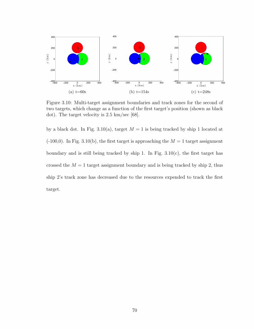
−400 −200 0 200 400−400

−200

0

200

400

x (km)

y(k

m)

1 2

33

1 2

(a) t=60s

−400 −200 0 200 400−400

−200

0

200

400

x (km)

y(k

m)

1 2

33

1 2

(b) t=154s

−400 −200 0 200 400−400

−200

0

200

400

x (km)

y(k

m)

1 2

33

1 2

(c) t=248s

Figure 3.10: Multi-target assignment boundaries and track zones for the second oftwo targets, which change as a function of the first target’s position (shown as blackdot). The target velocity is 2.5 km/sec [68].

by a black dot. In Fig. 3.10(a), target M = 1 is being tracked by ship 1 located at

(-100,0). In Fig. 3.10(b), the first target is approaching the M = 1 target assignment

boundary and is still being tracked by ship 1. In Fig. 3.10(c), the first target has

crossed the M = 1 target assignment boundary and is being tracked by ship 2, thus

ship 2’s track zone has decreased due to the resources expended to track the first

target.

70

Chapter 4

Consensus-based Optimization and Validation in Three Dimensions

This chapter presents a distributed, consensus-based approach to optimize the

radar resource allocation for ballistic missile surveillance and target tracking. Radar

search and target tracking consume resources as described in the three-dimensional

nonlinear physical radar model in Chapter 2. Target tracking includes an estimate

of the resources required to reduce target state uncertainty to a desired level to

support engagements. Each radar determines their preferred radar-to-target as-

signment using a probabilistic optimization algorithm that balances radar resource

loading and minimizes the total radar usage as described in Section 4.2. Under

heightened tracking demand, radar search resources may be reallocated to track as

described in Section 2.1.2 and search sectors degrade symmetrically about a des-

ignated threat axis. A unique global radar-to-target assignment that is robust to

resource estimation error is generated by a distributed consensus algorithm as de-

scribed in Section 4.3.

4.1 Optimization Approach

A two-stage approach is implemented to solve the target-assignment problem.

The first stage is a local optimization in which each radar finds a target-assignment

solution for the entire network that balances radar usage between radars and min-

71

imizes the total amount of radar usage among all radars. Radar resource usage

depends on the ballistic missile and air-defense search and track requirements as

well as resources required to reduce target uncertainty for engagements. Minimiz-

ing total resource usage among each radar allows for additional resources to be

applied to either search or track functions depending on the mission priorities as

described by a resource-allocation doctrine. Because of the binary structure of so-

lutions to the target-assignment problem (each target is assigned to exactly one

radar), graph-theoretic methods described in Section 2.3 are used to represent the

set of all possible target-assignment solutions. Due to the sheer number of candi-

date solutions that would have to be considered in an exhaustive search approach

for a large raid scenario, a probabilistic optimization algorithm known as a genetic

algorithm (GA) [8] is used to find the target-assignment solution that balances and

minimizes the total radar resource usage. GA’s maximize the fitness of a popula-

tion of chromosome-like candidate solutions using crossover, mutation, and other

evolution-inspired operations.

Two common approaches exist for multiple-objective optimization methods

using genetic algorithms [69]. The first approach, which is the approach taken in

this dissertation, combines the individual objective functions into a single compos-

ite function by selecting desired weights for each individual function. The second

approach determines an entire set of solutions that are non-dominated with respect

to each other. This set is known as a Pareto optimal set [69],[70]. Pareto optimal

sets may be preferred to single solutions when weights are difficult to determine or

if the trade-offs between each objective function are desired. However, the size of

72

the Pareto set increases with the number of objectives [70].

The second stage of the target-assignment problem requires inter-radar coordi-

nation. Radars repeatedly exchange and update their individual target-assignment

solutions over a balanced and strongly connected communication network in an it-

erative fashion that yields consensus on a single global solution. By using a theoret-

ically justified consensus control algorithm [9], the initial target-assignment solution

identified by each radar will be updated in such a way so as to reach an agreement

on a single solution.

The binary structure of the target-assignment solutions lends itself to a binary

consensus algorithm [37], [71] which has the additional benefit of being formulated

to be tolerant of communication noise and fading channels. Although reaching

consensus on the optimal target assignment may not always be necessary, since

the coordinating radars may all have access to the same optimization inputs, the

additional stage of reaching consensus among coordinating radars ensures that the

target-assignment process is robust to errors in resource estimation. These errors

arise because of the dynamic nature of the search resource allocation in the presence

of many targets—each radar may not know the search allocation of every other radar.

Consensus also provides robustness to inaccurate or unaccounted for sensor biases,

eliminates the possibility that a detected target is untracked when tracking resources

are available, and ensures that all radars share the same target-assignment solution

even in the presence of communication noise.

Using the radar and communication modeling framework outlined in Sec-

tion 2.3 and the target-assignment optimization and consensus algorithm from Sec-

73

tions 4.2 and 4.3, respectively, Section 4.4 demonstrates the improvement in radar

resource allocation and target tracking as compared to radars that are unable to

coordinate on their target-assignment using Monte Carlo simulations.

4.2 Target Assignment Optimization

This section presents the target assignment optimization framework for multi-

ple radars coordinating over a strongly connected, balanced communication network

with possibly directed links. It is assumed that each radar can accurately estimate

the position of every other radar using either GPS or other available sensors. All

radars implement a linear target tracking filter that uses the target measurements

in 2.13–2.18 to estimate the target state at each time step. Each radar broadcasts

the target state and uncertainty over the radar communication network and uses

this information in addition to an estimate of the other radars’ search resource usage

to optimize their target assignments. Because search resource usage is not usually

broadcast, each radar must estimate the search resource usage of other radars.

A target-assignment solution is the set of radar-to-target pairings that assigns

exactly one radar in the set N to each detected target in the disjoint set M, rep-

resented by the adjacency matrix of the bipartite graph Gtrack. The framework of

the target-assignment optimization problem is based upon meeting the following

two objectives: (i) balancing radar resource tasking and (ii) minimizing total radar

resource usage. Objectives (i) and (ii) are formulated using a quadratic form based

on a weighted graph Laplacian [61] that reflects the priorities of balancing resource

74

usage verses total resource usage. The solution to the optimization problem is the

target-assignment graph Gtrack that best achieves the convex combination of both

objectives.

For even a small number of targets, the exact solution to the problem obtained

by exhaustive search of each radar-to-target pairing yields excessive computational

time requirements since the number of possible pairings is NM . An alternate ap-

proach that achieves convergence to a near-optimal solution after considering dra-

matically fewer candidates is called a genetic algorithm (GA) [8]. A GA’s basic

principle is the maintenance of a population of individuals (genotypes) that evolve

over time based on the laws of natural selection and genetic information recombina-

tion [72]. Each individual represents a feasible solution of an optimization problem,

such as the target-assignment solution, and its objective function value is said to

be its fitness which is to be minimized (or maximized). The input to a genetic

algorithm is an initial population of randomly generated individuals. For each gen-

eration, every individual in the population is evaluated on their fitness, usually the

value of the objective function in the optimization problem being solved. The more

fit individuals are stochastically selected from the current population, and each in-

dividual’s genome is modified to form a new generation. The algorithm terminates

when either a maximum number of generations has been produced, or a satisfactory

fitness level has been reached for the population. A general genetic algorithm is

sketched in Table 4.1. While convergence results to the global optimal solution are

proven in [73] and [74], these results assume an elitist selection strategy (the best

individual survives with probability one). In [75], it is shown by means of homoge-

75

Table 4.1: Canonical Genetic Algorithm [75]choose an initial populationdetermine the fitness of each individualperform selectionrepeat

perform crossoverperform mutationdetermine the fitness of each individualperform selection

until stopping criterion applies

neous finite Markov chains that canonical genetic algorithms never converge to the

global optimum (though modified versions do).

A GA is used as opposed to alternatives like simulated annealing because

the discrete genome-like candidate solutions of ones and zeros closely resemble an

actual target-assignment pairing (i.e., the adjacency matrix of Gtrack). An initial

population of potential target- assignment graphs is encoded as a binary solution as

follows. Let Gtrack,k be the target-assignment solution proposed by radar k for all

radars and targets and let Ak ∈ RN×M be the adjacency matrix of Gtrack,k

such that

aij =

1, if Gtrack,k assigns target j to radar i

0, otherwise.

(4.1)

Note that Ak satisfiesN∑j=1

ajk = 1 which represents the constraint that each target is

assigned to exactly one radar and no (detected) targets are unassigned. Each local

target-assignment solution is evaluated based on the objective function described

below. New target-assignment graphs (offspring) are produced from pairs of current

graphs in the general population [76, pp. 211-231].

76

Objective (i) of the target-assignment optimization is to balance radar re-

sources over the radar communication network Gcom, (i.e., to minimize the dif-

ferences in radar usage between all pairs of communicating radars). Let P =

[P1 P2 ... PN ]T be the collection of all normalized (instantaneous) radar resource

allocations, where Pk , (T(tot)search,k + T

(tot)track,k + T

(tot)eng,k + εk)/Tmax denotes the total

normalized resources used for search and track by radar k. Let Lcom be the graph

Laplacian of Gcom. The optimal target-assignment network Gtrack balances radar

tasking across Gcom by minimizing the Laplacian quadratic form [12]

P TLcomP =∑

(j,k)∈Ecom

(Pk − Pj)2. (4.2)

Note the sum in 4.2 is over all edges (j,k) in Gcom. The quadratic form 4.2 represents

the level of disagreement in the radar resource usage, provided Gcom is a balanced

and strongly connected communication network.

Objective (ii) of the target-assignment optimization problem is to minimize the

total tracking resource usage over all radars in Gcom. Minimizing tracking resource

usage allows each radar to maximize the amount of resources available for BM

track and AD search. Let IN be the N × N identity matrix, which represents the

Laplacian of a balanced graph consisting of only self-loops, i.e. [lij] = 2 for all i = j,

and [lij] = 0 otherwise. (Note that a loop adds two to the degree matrix of a graph

since a vertex with a loop “sees” itself as an adjacent vertex from both ends of the

edge [61].) Minimizing total (squared) radar resources is equivalent to minimizing

77

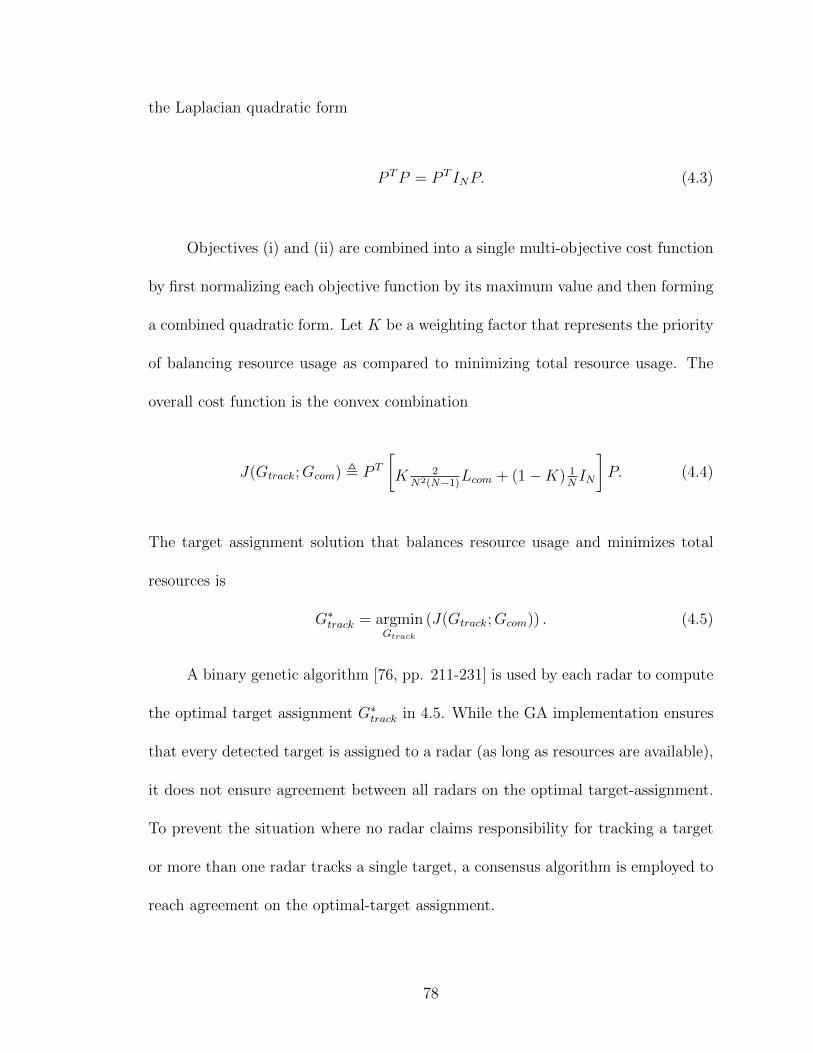
the Laplacian quadratic form

P TP = P T INP. (4.3)

Objectives (i) and (ii) are combined into a single multi-objective cost function

by first normalizing each objective function by its maximum value and then forming

a combined quadratic form. Let K be a weighting factor that represents the priority

of balancing resource usage as compared to minimizing total resource usage. The

overall cost function is the convex combination

J(Gtrack;Gcom) , P T

[K 2

N2(N−1)Lcom + (1−K) 1NIN

]P. (4.4)

The target assignment solution that balances resource usage and minimizes total

resources is

G∗track = argminGtrack

(J(Gtrack;Gcom)) . (4.5)

A binary genetic algorithm [76, pp. 211-231] is used by each radar to compute

the optimal target assignment G∗track in 4.5. While the GA implementation ensures

that every detected target is assigned to a radar (as long as resources are available),

it does not ensure agreement between all radars on the optimal target-assignment.

To prevent the situation where no radar claims responsibility for tracking a target

or more than one radar tracks a single target, a consensus algorithm is employed to

reach agreement on the optimal-target assignment.

78

4.3 Target Assignment Consensus

This section describes a consensus-based framework to reach agreement [9] on

target assignment, as represented by the adjacency matrix of the target-assignment

graph. Reaching consensus ensures exactly one common target assignment solution

and avoids the possibility that a target is not tracked. The consensus algorithm

described here also provides robustness to errors in radar resource estimation, track

uncertainty improvements, and communication noise. A binary consensus algorithm

is adopted, following [77] and [71], because of the binary nature of the target as-

signment solutions.

Let Gtrack,k be the target assignment solution initially proposed by radar k

using 4.5 and let Ak ∈ RN×M be the adjacency matrix of Gtrack,k as in 4.1. Define

Ak ∈ RNM×1 to be the elements of Ak taken column-wise and arranged as a single

column. Ak must be transmitted as a digital signal by radar k over Gcom, which

despite being balanced and strongly connected, may corrupt each transmission with

receiver noise. Let qjk(n) ∈ R represent the receiver noise at the nth time step in the

transmission of the target assignment solution from the kth radar to the jth one.

Because receiver noise typically has a flat power spectral density over the signal

band and a zero mean Gaussian voltage distribution [78, p. 946], the receiver noise

qjk(n) is assumed to be additive and zero-mean Gaussian with constance variance

σ2jk = σ2

w. (Each radar also has the same constant noise variance since identical

radars are considered, however the results also apply to varying and heterogenous

noise variances [77].)

79

Let Ajk(n) represent the reception of the target assignment at the jth radar

from the transmission of the kth one at the nth timestep, i.e., Ajk(n) = Ak(n) +

qjk(n), if (j, k) ∈ Ecom, where Ecom represents the set of radars in the edge set of

Gcom. Let Nj represent the set of radars k that can communicate with radar j

(including itself) and |Nj| be the size of Nj. Let Dec(·) denote a decision function

for the binary 0-1 entry performed on each element such that Dec(x) = 1 if x ≥ 0.5

and 0 otherwise. Each radar updates its own copy of the target assignment solution

based on the received information as follows [77]:

Aj(n+ 1) =Dec

1

1 + |Nj|

Aj(n)+∑

k∈Nj ,k 6=j

(Ak(n) + qjk(n))

. (4.6)

Note that 4.6 has the form of the consensus algorithm in 2.34, with x = A, ε =

1/(1 + |Nj)|, and Lcom = L. The advantage of working with binary consensus as

opposed to Euclidean consensus is that each node will reach consensus in finite time

verses infinite time. A noisy network is in accurate consensus at time step n if each

radar’s updated copy of the target assignment solution is equal to the noise-free

solution.

As shown in [77] and [71], the binary consensus algorithm 4.6 may be modeled

as a Markov Chain, where the transitional probabilities from one state to the next

are independent of the earlier states. Due to the presence of noise, there is no

guarantee in reaching or staying in consensus since the steady-state behavior is

independent of the initial state. However, the network can still achieve accurate

consensus for a certain period of time depending on the size of the network and the

80

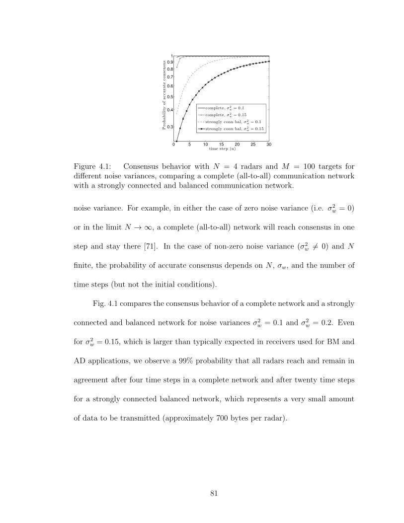
0 5 10 15 20 25 30

0.3

0.4

0.5

0.6

0.7

0.8

0.9

1

time step (n)

Pro

babilit

yof

accura

teconse

nsu

s

complete, σ2w = 0.1

complete, σ2w = 0.15

strongly conn bal, σ2w = 0.1

strongly conn bal, σ2w = 0.15

Figure 4.1: Consensus behavior with N = 4 radars and M = 100 targets fordifferent noise variances, comparing a complete (all-to-all) communication networkwith a strongly connected and balanced communication network.

noise variance. For example, in either the case of zero noise variance (i.e. σ2w = 0)

or in the limit N → ∞, a complete (all-to-all) network will reach consensus in one

step and stay there [71]. In the case of non-zero noise variance (σ2w 6= 0) and N

finite, the probability of accurate consensus depends on N , σw, and the number of

time steps (but not the initial conditions).

Fig. 4.1 compares the consensus behavior of a complete network and a strongly

connected and balanced network for noise variances σ2w = 0.1 and σ2

w = 0.2. Even

for σ2w = 0.15, which is larger than typically expected in receivers used for BM and

AD applications, we observe a 99% probability that all radars reach and remain in

agreement after four time steps in a complete network and after twenty time steps

for a strongly connected balanced network, which represents a very small amount

of data to be transmitted (approximately 700 bytes per radar).

81

Table 4.2: Multifunction array radar values used in simulations [45]

Radar Parameter Description Value

Pt Peak transmitted power (MW) 4

Pavg Average transmitted power (kW) 10

σ Target radar cross section (RCS) m2 1.0

Ae Effective Antenna Aperture (m2) 17.8

T0 Standard temperature (degrees K) 290

Fn Receive noise figure (dB) 6

Ls Total system losses (dB) 12

G Antenna gain (dB) 43.4

λ Wavelength (mm) 0.1

4.4 Performance Validation

Using the radar and communication modeling framework outlined in Chap-

ter 2, the improvement in radar resource allocation and target tracking as com-

pared to radars that are unable to coordinate on their target-assignment is demon-

strated using Monte Carlo simulations. Two different scenarios with four identical

radars, i.e. N = 4, are considered in which each radar maintains a pulse-repetition-

frequency of 100 update beams per second and performs volumetric searches over

BM sectors optimized about the predicted target trajectories. Target measurements

are updated every T = 2 seconds; radars optimize the target-assignment solution

and reach consensus every 4 seconds over a network with a communication latency

of Tcom = 6 seconds. For all search sectors, a maximum five-second search revisit

rate is instructed. The desired track uncertainty for engagement is 14.2 km which

is less than 0.15 seconds of error for a BM target traveling at 200 km/s [45]. Table

I lists the radar parameters used for both scenarios [45].

82

The target launch rate p(k) is modeled as a Poisson distribution p(k) =

(λk/k!)eλ, where λ is the expected number of targets launched every T = 2 sec-

onds and p(k) is the probability that k = 0, 1, 2, ... targets will be launched every

T seconds. BM raid size mean and standard deviation are shown in Fig. 4.2 for in-

creasing values of launch rate λ. Targets are detected with a single–look probability

of detection of 0.9 after they penetrate one of the ballistic missile search sectors [4].

Coordinated radars broadcast the target state and uncertainty over the radar com-

munication network Gcom shown in Fig. 2.9, solve for optimal target-assignment

using 4.5, and use this solution to initialize the binary consensus algorithm 4.6. The

consensus algorithm uses Gcom with noise variance σ2w = 0.1.

Coordinated radars are compared with two types of uncoordinated radars:

Independent radars and Shared radars [79]. In the Independent case, each radar

only tracks targets that are detected within its own search sector. In the Shared

case, each radars may track a target detected by a neighboring radar but radars do

not optimize the target assignment. Thus in the Shared case more than one radar

may track the same target.

4.4.1 Scenario 1: Short-range BM Raid

The first scenario considers a short range (< 500 km) BM raid. Each target has

maximum life span of 300 seconds and vanishes on impact. Targets trajectories are

chosen from a set of four launch points and two aim points with a larger percentage

of the targets coming from the two launch points located near (0,0) as shown in

83

Fig. 4.3. Fig. 4.3 also plots the location of each radar with respect to the aim points

0 1 2 30

50

100

150

200

250

300

Raid rate (λ)

Num

ber

of

targ

ets

Figure 4.2: The total number of launched targets (mean and standard deviation)increases with the raid rate λ (expected number of targets launched every T = 2seconds).

(denoted by the black X’s). The ellipses around the aim points describe the 2σ

ellipses of the impact point probability distribution.

Figs. 4.4(a), 4.4(c), and 4.4(e) plot the mean-centered standard deviation of the

total normalized resource usage obtained from 30 Monte Carlo trials with a variable

resource allocation doctrine, a launch rate of λ = 0.5, and K = 0.5. This value of K

implies minimizing radar resource usage has the same priority as balancing resource

usage. (Recall a variable resource allocation doctrine implies that once resources

initially reserved for BM track are depleted, AD search resources may be converted

to BM track.) In this case the remaining AD search resources are re-optimized to

ensure that the search sector is centered on the expected AD threat axis. Note that

on average, Coordinated radars use less total resources than both the Independent

and Shared radars throughout the scenario. Figs. 4.4(b), 4.4(d), and 4.4(f) plot the

total pairwise difference in radar usage for all three cases. Throughout the entire

84

Figure 4.3: Scenario 1 radar locations and BM search sectors with respect to thetarget launch and impact point distributions.

scenario, the maximum pairwise difference for Coordinated radars is less than the

maximum pairwise difference for both Independent and Shared radars, indicating

superior load balancing as compared to the uncoordinated alternatives. Figs. 4.5(a)–

4.5(b) plot the maximum mean value of the total normalized radar resource usage

and the mean of the sum of pairwise differences in resource usage for Coordinated

radars over a range of launch rates λ and gains K. Note that smaller values of K result

in less total resource usage as compared to larger values of K, which result in a more

balanced resource utilization as expected. To highlight the benefit of coordination in

terms of reducing the number of missed targets, Figs. 4.5(c)–4.5(f) plot the mean-

centered standard deviation (grey bar) and single radar worst-case (dotted-line)

total resource usage and sum of pairwise difference in resource usage statistics from

the Monte Carlo simulations for all raid rates and a fixed value K = 0.6 for both

85

Coordinated and Independent radars. (Shared radars are not plotted since their

maximum resource usage is equal to one for all raid rates.) While the Independent

radars are observed to use less average resources due to their lack of coordination,

their resource usage is unbalanced across the network and leads to a greater number

of missed targets as shown in Table 4.3.

Table 4.3: Scenario 1: Total Number of Missed Targets for K = 0.5

λ = 0.5 λ = 1.0 λ = 1.5 λ = 2.0

Coordinated 0 0 1 14

Independent 0 0 4 38

Shared 11 51 79 94

4.4.2 Scenario 2: Medium-range BM Raid

The second scenario considers a raid of medium range (≈ 1500 km) ballistic

missiles. Radars are stationed farther from the launch points and impact points

as compared to Scenario 1 (see Fig. 4.6). The goal of this scenario is to stress the

resource requirement for both tracking and engagements due to the increased target

range from each radar. While each target has a total life expectancy of 600 seconds,

targets are tracked until they reach apogee altitude at 350 km and the total scenario

time is limited to 200 seconds due to radar resource saturation. Targets trajectories

are chosen from the same set of four launch points and two different aim points

with a larger percentage of the targets coming from the two launch points located

near (0,0). Fig. 4.6 also plots the location of each radar with respect to the aim

points (denoted by the black X’s). The ellipses around the aim points describe the

86

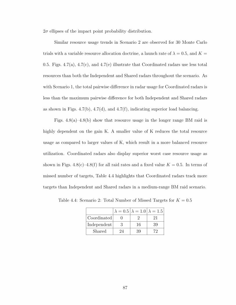
2σ ellipses of the impact point probability distribution.

Similar resource usage trends in Scenario 2 are observed for 30 Monte Carlo

trials with a variable resource allocation doctrine, a launch rate of λ = 0.5, and K =

0.5. Figs. 4.7(a), 4.7(c), and 4.7(e) illustrate that Coordinated radars use less total

resources than both the Independent and Shared radars throughout the scenario. As

with Scenario 1, the total pairwise difference in radar usage for Coordinated radars is

less than the maximum pairwise difference for both Independent and Shared radars

as shown in Figs. 4.7(b), 4.7(d), and 4.7(f), indicating superior load balancing.

Figs. 4.8(a)–4.8(b) show that resource usage in the longer range BM raid is

highly dependent on the gain K. A smaller value of K reduces the total resource

usage as compared to larger values of K, which result in a more balanced resource

utilization. Coordinated radars also display superior worst case resource usage as

shown in Figs. 4.8(c)–4.8(f) for all raid rates and a fixed value K = 0.5. In terms of

missed number of targets, Table 4.4 highlights that Coordinated radars track more

targets than Independent and Shared radars in a medium-range BM raid scenario.

Table 4.4: Scenario 2: Total Number of Missed Targets for K = 0.5

λ = 0.5 λ = 1.0 λ = 1.5

Coordinated 0 2 21

Independent 3 16 39

Shared 24 39 72

87

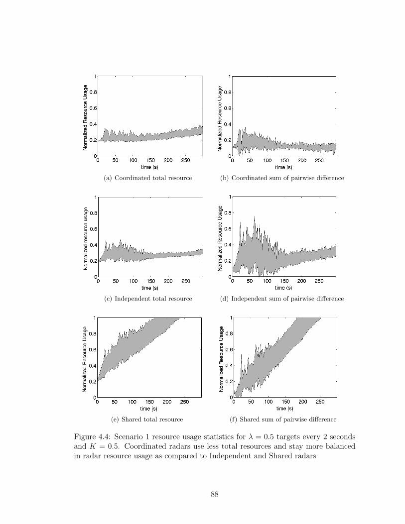
(a) Coordinated total resource (b) Coordinated sum of pairwise difference

(c) Independent total resource (d) Independent sum of pairwise difference

(e) Shared total resource (f) Shared sum of pairwise difference

Figure 4.4: Scenario 1 resource usage statistics for λ = 0.5 targets every 2 secondsand K = 0.5. Coordinated radars use less total resources and stay more balancedin radar resource usage as compared to Independent and Shared radars

88

0 0.2 0.4 0.6 0.8 1

0.4

0.5

0.6

0.7

0.8

0.9

1

K

Norm

ali

zed

Res

ourc

eU

sage

λ = 0.5

λ = 1.0

λ = 1.5

λ = 2.0

(a) Coordinated total resource

0 0.2 0.4 0.6 0.8 10.05

0.1

0.15

0.2

0.25

0.3

0.35

0.4

K

Norm

ali

zed

Res

ourc

eU

sage

λ = 0.5

λ = 1.0

λ = 1.5

λ = 2.0

(b) Coordinated sum of pairwise difference inresource

0.5 1 1.5 20

0.2

0.4

0.6

0.8

1

λ

No

rma

lize

d R

eso

urc

e U

sa

ge

Standard Deviation

Worst Case

(c) Coordinated total resource

0.5 1 1.5 20

0.2

0.4

0.6

0.8

1

λ

No

rma

lize

d R

eso

urc

e U

sa

ge

Standard Deviation

Worst Case

(d) Independent total resource

0.5 1 1.5 20

0.2

0.4

0.6

0.8

1

λ

No

rma

lize

d R

eso

urc

e U

sa

ge

Standard Deviation

Worst Case

(e) Coordinated sum of pairwise difference in re-source

0.5 1 1.5 20

0.2

0.4

0.6

0.8

1

λ

No

rma

lize

d R

eso

urc

e U

sa

ge

Standard Deviation

Worst Case

(f) Independent sum of pairwise difference in re-source

Figure 4.5: (a)–(b) illustrate the total resource usage and sum of pairwise resourceusage dependence on gain K for all raid rates λ; (c)–(f) highlight the increase totalresource usage and the sum of the pairwise difference in resource usage with largerraid rates. Note that, regardless of the raid rate, the worst case radar usage forCoordinated radars is less than Independent and Shared radars (not shown).

89

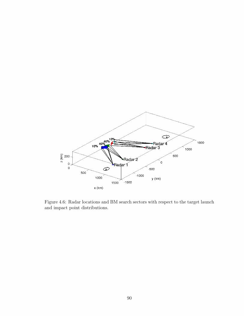
Figure 4.6: Radar locations and BM search sectors with respect to the target launchand impact point distributions.

90

(a) Coordinated total resource (b) Coordinated sum of pairwise difference

(c) Independent total resource (d) Independent sum of pairwise difference

(e) Shared total resource (f) Shared sum of pairwise difference

Figure 4.7: Scenario 2 resource usage statistics for λ = 0.5 targets every 2 secondsand K = 0.5. Coordinated radars use less total resources and stay more balancedin radar resource usage as compared to Independent and Shared radars

91

0 0.2 0.4 0.6 0.8 10.5

0.6

0.7

0.8

0.9

1

K

Norm

ali

zed

Res

ourc

eU

sage

λ = 0.5

λ = 1.0

λ = 1.5

(a) Coordinated total resource

0 0.2 0.4 0.6 0.8 10

0.05

0.1

0.15

0.2

0.25

0.3

0.35

0.4

K

Norm

ali

zed

Res

ourc

eU

sage

λ = 0.5

λ = 1.0

λ = 1.5

(b) Coordinated sum of pairwise difference in re-source

0.5 1 1.50

0.2

0.4

0.6

0.8

1

λ

No

rma

lize

d R

eso

urc

e U

sa

ge

Standard Deviation

Worst Case

(c) Coordinated total resource

0.5 1 1.50

0.2

0.4

0.6

0.8

1

λ

No

rma

lize

d R

eso

urc

e U

sa

ge

Standard Deviation

Worst Case

(d) Independent total resource

0.5 1 1.50

0.2

0.4

0.6

0.8

1

λ

No

rma

lize

d R

eso

urc

e U

sa

ge

Standard Deviation

Worst Case

(e) Coordinated sum of pairwise difference in re-source

0.5 0.6 0.7 0.8 0.9 1 1.10

0.2

0.4

0.6

0.8

1

λ

No

rma

lize

d R

eso

urc

e U

sa

ge

Standard Deviation

Worst Case

(f) Independent sum of pairwise difference in re-source

Figure 4.8: (a)–(b) illustrate the total resource usage and sum of pairwise resourceusage dependence on gain K for all raid rates λ; (c)–(f) highlight the increase totalresource usage and the sum of the pairwise difference in resource usage with largerraid rates. Note that, regardless of the raid rate, the worst case radar usage forCoordinated radars is less than Independent and Shared radars (not shown).

92

Chapter 5

Conclusions

5.1 Summary of Dissertation

Distributed optimization of radar resource allocation addresses the problem of

effectively managing the limited resources among a networked multifunction radars

to accomplish a prioritized list of search and track functions. This dissertation

has contributed to the design of a conceptual architecture and framework for the

distributed resource coordination of multifunction radar systems.

Starting with two-dimensional linear and nonlinear radar models, a distributed

search-area optimization algorithm is described that maximizes the collective search

area of identical shipboard multifunction radar systems in which some or all of the

systems are able to coordinate on their tasking. Analytical results show that the

search-area optimization algorithm increases the combined search area of two and

three ships over the uncoordinated combined search area in a directed network

modeled using graph theory. An optimal target-assignment algorithm is presented

that balances the radar tasking for radars that are both optimized and unoptimized

with respect to their search area. For radars that coordinate on their target as-

signment, the solution to the target assignment problem is a hyperbolic boundary

determined by the radar surveillance requirements, range to the target, and current

target tasking. The proposed solutions are validated by a combination of analytical

93

and numerical results using a simulated annealing algorithm.

Using a three-dimensional nonlinear radar model, a distributed, consensus-

based optimization approach to manage radar resources is described for ballistic mis-

sile and air-defense surveillance and target tracking. A target-assignment optimiza-

tion algorithm that uses a binary genetic algorithm to balance and minimize radar

resource usage across the radars in the network is presented. Radar resources include

the additional resources required to reduce track uncertainty in support of engage-

ments. Remaining air-defense search resources are optimized about a projected

threat-axis by employing a simulated annealing algorithm. Radar reach agreement

on the optimal target-assignment using a binary consensus algorithm. Monte Carlo

simulations demonstrate that the consensus-based distributed target-assignment ap-

proach uses less overall resources and remains more balanced in resource usage than

uncoordinated alternatives, thus increasing the number of additional targets that

may detected and tracked.

5.2 Suggestions for Future Research

Optimization of sensor resource management can lead to many different ap-

proaches and tradeoffs. While this dissertation has advanced the state of the art in

multifunction radar resource coordination for ballistic missile and air-defense surveil-

lance and target tracking, it has also highlighted various focus areas for future work.

The 3D nonlinear radar model considered in Chapter 2 can be improved in

fidelity by considering radar power requirements as an additional dynamic resource

94

constraint and tradeoff [80]. Maneuvering targets would add another level of com-

plexity to the target-assignment optimization problem as additional tracking re-

sources would be required to increase the target measurement update rate to main-

tain a desired level of track accuracy [81], [82]. Additional tracking considerations

such as including imperfect data associations [57],[83] and tracking in clutter are

expected to affect the track uncertainty, however accurately translating these ad-

ditional considerations to a radar time-resource loading requirement requires ad-

ditional research [80] . Certainly the more complicated the threat environment,

the more adaptable and robust the radar resource manager must be to determine

the proper resource to task allocation in order to maintain an accurate situational

awareness picture.

The dynamic load balancing and load minimization approach has demon-

strated improved performance over the uncoordinated alternative strategies for BM

target tracking and to a lesser extent air-defense surveillance. However, these func-

tions represent only two of the many functions that a multifunction radar systems

performs. Indeed the greatest benefit of the radar itself is its ability to perform

many different functions that previously required separate radars. To that end, the

balancing and minimizing approach could be extended to tracking air- and surface

targets as well as long-range search. Radar functions such as track initiation, target

discrimination, and engagement assessment are functions that were not considered

as part of this thesis but may consume a large amount of radar resources depending

on the mission and tasking priorities. Optimizing the sensor placement to balance

and minimize the radar resource usage for search and anticipated target tracking

95

seems to be another relevant extension of our existing work.

The implementation of the target-assignment optimization algorithm presented

in this dissertation can be improved. The genetic algorithm provides a computation-

ally efficient method to solve for a local optimal solution in a significantly reduced

timeframe as compared to an exhaustive search. However, there may exist alterna-

tive optimization algorithms that converge to a global optimal solution in less time

than the genetic algorithm implemented here. While all the computations required

for the Monte Carlo simulations were performed on a standard laptop computer, the

target models and threat environment were less complex than would be observed in

reality. Thus using real target and radar data would be of benefit to compare the

computational performance of the target-assignment optimization algorithm within

the framework of radar’s data processing timeline and communication latency.

Consideration of non-homogenous radars should be a next step in further-

ing this research. Sensors other than radars that can provide an estimate of their

resource usage for surveillance and target tracking should also be considered and

would provide a logical extension of the existing radar modeling framework.

96

Appendix A

Search-Area Maximization Analytical Results

For completeness the proofs of the Lemmas 1–9 from Section 3 are presented.

Proof of Lemma 1

Since f(ρ) monotonically increases with ρ and α > 0, then ρ∗ satisfies 3.6=0.

Proof of Lemma 2

The distance between the two ships as a function of the search radius ρ and

angle of overlap θ is found by solving 3.10 for δ to obtain

δ∗ ≈ ρ

(2− θ2

4

). (A.1)

Using 3.11, the optimality condition g(ρ∗, δ∗) = 0 is satisfied when

θ =αρ∗ + β

a. (A.2)

Substituting A.2 into A.1 yields 3.13.

Since 3.8 is maximized for small values of θ, a Taylor series expansion of sin θ

97

about θ = 0 is performed in 3.8, which yields

f(ρ, δ) ≈ 2πρ2 − θ3ρ2

6. (A.3)

The derivative of A.3 with respect to ρ is

∂f

∂ρ= 4πρ− 1

3θ3ρ− 1

2ρ2θ2

∂θ

∂ρ. (A.4)

A.4 is written in terms of ρ using A.2 and ∂θ/∂ρ = α/a. The final equation

is a quartic function in ρ with a degenerate root equal to 0, leaving the cubic

polynomial 3.12. As a consequence of the intermediate value theorem [84], 3.12 has

at least one solution among the real numbers because the degree of the polynomial

is odd. Because its discriminant

∆ = 18b1b2b3b4 − 4b33b1 + b23b22 − 4b4b

22 − 27b24b

21 (A.5)

is positive, there exists three real roots. The largest root is chosen to maximize A.3,

which completes the proof.

Proof of Lemma 3

From Lemma 2, the objective function is given by A.3 where θ = (αρ∗ + β)/a

as in A.2 for the optimality condition g(ρ∗, δ) = 0. Substituting A.2 into A.1 with

98

δ∗ = δ yields

δ ≈ ρ∗

(2−

(αρ∗ + β

2b

)2). (A.6)

Solving A.6 for ρ∗ yields 3.12, which completes the proof.

It was shown in Lemma 3 that given the position of two ships with equal radii,

one can solve for the maximum search radius for each radar. Note that in order to

satisfy the optimality condition g(ρ∗, δ) = 0, each ship position must satisfy A.6 for

at least one real root ρ∗. Choosing δ ≤ 2ρ1 where ρ1 = ρ∗ from the optimal N = 1

search radius ensures a solution to A.6.

Proof of Lemma 4

Let ρ1 = ρ∗ (the N = 1 optimal radius). The objective function is given

by 3.24, where θ1,2 and θ2,1 are as in 3.19 and 3.20 respectively and δ1,2 = δ ≤

2(ρ∗ + ρ2). To satisfy the N = 2 sensor overlap requirement and to avoid solving

first for δ∗, δ is chosen such that δ ≤ 2ρ∗. 3.24 is maximized when

αρ2 + β − 2a

√2

(1− δ2 − ρ∗2 + ρ22

2δρ2

)= 0. (A.7)

Solving A.7 for ρ2 yields 3.26, which completes the proof.

Proof of Lemma 5

Since each ship is equally spaced with equal radar search radii, the optimal

distance δ∗ is found by solving 3.11 for the optimality condition g(ρ∗, δ∗) = 0.

99

Substituting A.2 into A.1 yields A.6. The combined search area given by 3.27 can

be expressed as

f(ρ, δ) =

(3

2π − θ + sin θ

)2ρ2, (A.8)

where θ1,2 = θ2,1 = θ2,3 = θ3,2 = θ and θ1,3 = θ3,1 = 0 (since shipboard radars 1 and

3 do not overlap in coverage area). A.8 is maximized for small overlap angle θ, thus

a Taylor series expansion of sin θ is performed about θ = 0 in A.8 to obtain

f(ρ, δ) ≈ 3πρ2 − θ3ρ2

3. (A.9)

Taking the derivative of A.9 with respect to ρ yields

∂f

∂ρ= 6πρ− 2

3θ3ρ− ρ2θ2∂θ

∂ρ. (A.10)

A.10 is written in terms of ρ using θ = (αρ∗ + β)/a and ∂θ/∂ρ = α/a. The final

equation is a quartic function of ρ with a degenerate root equal to 0, leaving the

cubic polynomial 3.12 with its discriminant A.5 greater than zero. Thus there exists

three real roots and the largest root is chosen to maximize A.9, which completes the

proof.

Proof of Lemma 6

From Lemma 5, the objective function is given by A.9 where θ = (αρ∗ + β)/a

as in A.2 for the optimality condition g(ρ∗, δ) = 0. Substituting A.2 into A.1 with

δ∗ = δ yields A.6. Solving A.6 for ρ∗ yields 3.12, which completes the proof.

100

Proof of Lemma 7

As in Lemma 4, let ρ2 = ρ∗ from Lemma 1. Then

θ1,2 ≈ 2

√2

(1− δ2 + ρ12 − ρ∗2

2δρ1

)(A.11)

θ2,1 ≈ 2

√2

(1− δ2 + ρ∗2 − ρ12

2δρ∗

)(A.12)

θ2,3 ≈ 2

√2

(1− δ2 + ρ∗2 − ρ23

2δρ∗

)(A.13)

θ3,2 ≈ 2

√2

(1− δ2 + ρ32 − ρ∗2

2δρ3

). (A.14)

The combined search area 3.27 becomes

f(ρ1, ρ2, ρ3, δ) =

(π +

(sin θ1,2 − θ1,2

2

))ρ21

+

(π +

(sin θ2,1 − θ2,1

2+

sin θ2,3 − θ2,32

))ρ22

+

(π +

(sin θ3,2 − θ3,2

2

))ρ23. (A.15)

A.15 is maximized when the overlap angle for each ship pair, θj,k, is small, thus a

Taylor series expansion of sin θj,k is performed about θj,k = 0 in A.15 to obtain

f(ρ1, ρ2, ρ3, δ) ≈ (2π −θ31,26

)ρ212

+ (2π −θ32,16−θ32,36

)ρ∗2

2

+ (2π −θ33,26

)ρ232. (A.16)

It follows from Lemma 4 that A.16 is maximized for the optimality condition

g(ρk, δ) = 0. Given the spacing δ between each adjacent ship pair and ρ2 = ρ∗,

101

A.11 is solved for ρ1 and A.14 for ρ3 with θ1,2 = (αρ1 +β)/a and θ3,2 = (αρ3 +β)/a,

which yields 3.26 and completes the proof.

Proof of Lemma 8

For Scenario 2 there exists no common overlap area for all three radars. In

addition, since all radars have equal radii and separation, the overlap angles between

each radar pair, θj,k, are equal, i.e. θ1,2 = θ2,1 = θ2,3 = θ3,2 = θ1,3 = θ3,1. The

combined search area 3.27 is expressed as

f(ρ, δ) = 3πρ2 − 3θρ2 + 3 sin θρ2, (A.17)

where θ equals the total overlap angle for each individual ship, i.e., θ1 = θ1,2 + θ1,3

and θ1 = θ2 = θ3 = θ. A.17 is maximized when the overlap angle for each ship pair

is small, thus a Taylor series expansion of sin θ is performed about θ = 0 in A.17 to

obtain

f(ρ, δ) = 3πρ2 − θ3ρ2

2. (A.18)

The distance between each ship pair is expressed as a function of the search radius

ρ and pairwise angle of overlap θj,k by solving 3.10 for δ. Using 3.11, the optimality

condition g(ρ∗, δ) = 0 is satisfied for A.2, where θ is the sum of each pairwise angle

of overlap, i.e. θ1 = θ1,2 + θ1,3 = 2θ1,2. Substituting θ/2 into A.6 yields 3.12 and

completes the proof.

102

Proof of Lemma 9

The optimal distance between all three ships follows from Lemma 2 and Lemma

8. Taking the derivative of A.18 with respect to ρ yields

∂f

∂ρ= 6πρ− θ3ρ2 − 3

2θ2ρ2

∂θ

∂ρ. (A.19)

A.19 is written in terms of ρ using A.2 with ∂θ/∂ρ = α/a The rest of the proof

follows the proof of Lemma 2.

103

Bibliography

[1] (2006, July). [Online]. Available: http://news.bbc.co.uk/2/hi/asia-pacific/5152918.stm

[2] [Online]. Available: http://www.mda.mil/system/system.html

[3] S. Sabatini and M. Tarantino, Multifunction Array Radar - System Design andAnalysis. Artech House, 1994.

[4] M. Skolnik, Introduction to Radar Systems, 3rd ed. McGraw-Hill, 2001.

[5] S. Miranda, C. Baker, K. Woodbridge, and H. Griffiths, “Knowledge-basedresource mangement for multifunction radar,” in IEEE Signal Processing Mag-azine, 2006.

[6] B. Weir and T. Sokol, “Radar coordination and resource management in adistributed sensor network using emergent control,” in Proc. of SPIE, vol. 7350,2009.

[7] [Online]. Available: http://tinyurl.com/lqjeff2

[8] C.M.Fonseca and P. Fleming, “Genetic algorithms for multiobjective optimiza-tion: Formulation, discussion and generalization,” in Proc. 5th Int. Conf. Ge-netic Algorithms, 1993, pp. 416–423.

[9] R. Saber and R. Murray, “Consensus and cooperation in networked multi-agentsystems,” in Proceedings of the IEEE, vol. 95, Jan 2007, pp. 215–223.

[10] W. Ren, R. Beard, and E. Atkins, “A survey of consensus problems in multi-agent coordination,” American Control Conference, pp. 1859–1864, June 2005.

[11] W. Ren and R. Beard, “Consensus seeking in multi-agent systems under dy-namically changing interaction topologies,” in IEEE Trans. Autom. Control,vol. 50, May 2005, pp. 655–661.

[12] R. Saber and R. Murray, “Consensus problems in networks of agents withswitching topology and time-delays,” IEEE Transactions on Automatic Con-trol, vol. 49, no. 9, September 2004.

[13] A. Hero and D. Cochran, “Sensor management: Past, present, and future,” inIEEE Sensors Journal, vol. 11, no. 12, 2011, pp. 3064–3075.

[14] D. J. Kershaw and R. J. Evans, “Optimal waveform selection for tracking sys-tems,” in IEEE Trans. Inform. Theory, vol. 40, no. 5, Sep 1994, pp. 1536–1550.

[15] ——, “Waveform selective probabilistic data association,” in IEEE Trans.Aerosp. Electron. Syst., vol. 33, no. 4, Oct 1997, pp. 1180–1188.

104

[16] S. Sowelam and A. H. Tewfik, “Optimal waveform selection in range-dopplerimaging,” in Proc. IEEE Int. Conf. Image Process, Nov 1994, pp. 441–445.

[17] S. M. Sowelam and A. H. Tewfik, “Optimal waveform selection for radar targetclassification,” in Proc. IEEE Int. Conf. Image Process, Oct 1997, pp. 476–479.

[18] S. Ghosh, J. Hansen, R. Rajkumar, and J. Lehoczky, “Integrated resourcemanagement and scheduling with multi-resource constraints,” in Proceedingsof the 25th IEEE International Real-Time Systems Symposium, 2004, pp. 12–22.

[19] A. Charlish, K. Woodbridge, and H. Griffiths, “Multi-target tracking controlusing continuous double auction parameter selection,” in Proc. of the 15th In-ternational Conf on Information Fusion, 2012, pp. 1269–1276.

[20] N. Goodman, P. Venkata, and M. Neifeld, “Adaptive waveform design andsequential hypothesis testing for target recognition with active sensors,” inIEEE. J. Select. Topics Signal Process., vol. 1, no. 1, Jun 2007, pp. 105–113.

[21] S. Sira, Y. Li, A. Papandreou-Suppappola, D. Morrell, D. Cochran, andM. Rangaswamy, “Waveform-agile sensing for tracking,” in IEEE. Signal Pro-cess. Mag., vol. 26, no. 1, 2009 2009, pp. 53–64.

[22] A. Leshem, O. Naparstek, and A. Nehorai, “Information theoretic adaptiveradar waveform design for multiple-extended targets,” in IEEE J. Select TopicsSignal Process., vol. 1, no. 1, Jun 2007, pp. 42–55.

[23] A. Izquierdo-Fuente and J. Casar-Corredera, “Optimal radar pulse schedulingusing a neural network,” in IEEE Int. Conf on Neural Networks, vol. 7, 1994,pp. 4588–4591.

[24] V. Krishnamurthy and D. Djonin, “Optimal threshold policies for multivariatePOMDPs in radar resource management,” in IEEE Trans. Signal Process.,vol. 57, no. 10, Oct. 2009, pp. 3954–3969.

[25] J. Nino-Mora and S. Villar, “Multitarget tracking via restless bandit marginalproductivity indices and kalman filter in discrete time,” in Joint 48th IEEEConf. on Decision and Control and 28th Chinese Control Conf., Dec. 2009, pp.2905–2909.

[26] B. F. L. Scala and B. Moran, “Optimal target tracking with restless bandits,”in Digital Signal Process., vol. 16, no. 5, 2006 2006, pp. 479–487.

[27] D. Khosla and J. Guillochon, “Distributed sensor resource management andplanning,” in Proc. of SPIE on Signal Processing, Sensor Fusion, and TargetRecognition, vol. 6567, 2007.

105

[28] S. Sinno and D. Kreithen, “A constrained joint optimization approach to dy-namic sensor configuration,” in Conf. Record of the 36th Asilomar Conf onSignals, Systems and Computers, vol. 2, 2002, pp. 1179–1183.

[29] M. Kalandros and L. Pao, “Covariance control for multisensor systems,” inIEEE Transactions on Aerospace and Electronic Systems, 2002, pp. 1138–1157.

[30] C. Kreucher, K. Kastella, and A. O. Hero, “Information based sensor manage-ment for multitarget tracking,” in Proc. of SPIE on Signal and Data Process.of Small Targets, vol. 5204, 2003, pp. 480–489.

[31] A. Renyi, “On measures of entropy and information,” in Proc. 4th BerkeleySymp. Math. Stat. and Prob., vol. 1, 1961, pp. 547–561.

[32] C. Schumacher, P. Chandler, and S. Rasmussen, “Task allocation for wide areasearch munitions,” in Proceedings of the American Control Conference, 2002,pp. 1917–1922.

[33] S. L. Smith and F. Bullo, “Monotonic target assignment for robotic networks,”IEEE Transactions on Automatic Control, vol. 54, no. 9, pp. 2042–2057, 2009.

[34] K. J. Obermeyer, A. Ganguli, and F. Bullo, “A complete algorithm for search-light scheduling,” International Journal of Computational Geometry and Ap-plications, vol. 21, no. 1, pp. 101–130, October 2011.

[35] P.-S. Kang and C.-G. Lee, “Coordinated search and track by multiple phasedarray radars,” in 10th IEEE Real-Time and Embedded Technology and Appli-cations Symposium, no. 10. IEEE Computer Society, 2004, pp. 227–235.

[36] H. Lambert and D. Sinno, “Bioinspired resource management for multiple-sensor target tracking systems,” M.I.T., Tech. Rep., 2011.

[37] Y. Mostofi and M. Malmirchegini, “Binary consensus over fading channels,” inIEEE Trans. on Signal Processing, vol. 58, no. 12, 2010, pp. 6340–6353.

[38] D. R. Billetter, Multifunction Array Radar. Artech House, 1989.

[39] A. Charlish, “Autonomous agents for multi-function radar resource manage-ment,” Ph.D. dissertation, Univ. College London, 2011.

[40] C. Scott, “The neyman-pearson criterion.”

[41] M. Richards, Fundamentals of Radar Signal Processing. McGraw-Hill, NewYork, 2005.

[42] T. Jeffrey, Phased Array Radar Design. SciTech Publishing, Inc., 2009.

[43] T. W. Jeffrey, “Track quality estimation for multiple-target tracking radars,”in Proc. of 1989 Nation Radar Conf., 1989, pp. 76–79.

106

[44] M. Skolnik, Radar Handbook, 3rd ed. McGraw-Hill, 2008.

[45] C.Bacchus, D. Bedford, P. Dailey, S. Hill, I.Barford, J.Chung, R. Hazle, andM. Mihocka, “Digital array radar for ballistic missile defense and counter-stealth systems analysis and parameter tradeoff study,” Naval PostgraduateSchool, Tech. Rep. SE-06-001, 2006.

[46] E. W. Weisstein. Solid angle. [Online]. Available: http://mathworld.wolfram.com/SolidAngle.html

[47] D. Bertsimas and J. Tsitsiklis, “Simulated annealing,” Statistical Science, vol. 8,no. 1, pp. 10–15, 1993.

[48] A. Levitin, Introduction to the Design and Analysis of Algorithms, 3rd ed.Addison-Wesley, 2011.

[49] D. S. Hochbaum, “Complexity and algorithms for nonlinear optimization prob-lems,” Annals of Operations Research, vol. 153, no. 1, pp. 257–296, 2007.

[50] G. H. Sasaki and B. Hajek, “The time complexity of maximum matching bysimulated annealing,” Journal of the ACM, vol. 35, pp. 387–403, 1988.

[51] D. Mitra, F. Romeo, and A. Sangiovanni-Vincentelli, “Convergence and finite-time behavior of simmulated annealing,” in Advances in Applied Probability,1986, pp. 747–771.

[52] D. Henderson, S. Jacobson, and A. Johnson, The theory and practice of simu-lated annealing. Handbook of metaheuristics, 2003, pp. 287–319.

[53] A. Farina, B. Ristic, and D. Benvenuti, “Tracking a ballistic target: Comparisonof several nonlinear filters,” in IEEE Transactions on Aerospace and ElectronicSystems, 2002, pp. 854–867.

[54] K. V. Ramachandra, Kalman Filtering Techniquest for Radar Tracking. MarcelDekker, Inc., 2000.

[55] A. Farina, M. D. Gaudio, U. D’Elia, S. Immediata, and L. Ortenzi, “Detectionand tracking of ballistic target,” in Proc. of the IEEE Radar Conf, 2004, pp.450–456.

[56] X. R. Li and V. P. Jilkov, “A survey of maneuvering target tracking - part ii:Ballistic target models,” in Proc. of SPIE Conf on Signal and Data Processingof Small Targets, 2001.

[57] Y. Bar-Shalom, Ed., Multitarget-Multisensor Tracking: Advanced Applications.Artech House, 1990.

[58] S. S. Blackmann, Multiple-Target Tracking with Radar Applications. ArtechHouse, 1986.

107

[59] D. Lerro and Y. Bar-Shalom, “Tracking with debiased consistent convertedmeasurements versus ekf,” in IEEE Transactions on Aerospace and ElectronicSystems, 1993, pp. 1015–1022.

[60] J. Mingrone and M. L. Venuti, Track Quality to Track Error Covariance, Lock-heed Martin Corporation, http://www.freepatentsonline.com/8052054.html,2001.

[61] C. Godsil and G. Royle, Algebraic Graph Theory. Springer, 2001.

[62] N. Biggs, Algebraic Graph Theory, 2nd ed. Cambridge University Press, 1993.

[63] R. Diestel, Graph Theory, Grad. Texts in Math. Springer, 2005.

[64] N.J.Harvey, R. Ladner, L. Lovasz, and T. Tamir, “Semi-matchings for bipartitegraphs and load balancing,” in Workshop of Algorithms and Data Structures,2003.

[65] K. Cai and H. Ishii, “Average consensus on general strongly connected di-graphs,” in Proc. of the 28th American Control Conference (ACC), 2012, pp.14–19.

[66] ——, “Quantized consensus and averaging on gossip digraphs,” in IEEE Trans.Autom. Control, vol. 56, no. 9, Sept 2011, pp. 2087–2100.

[67] M. Fewell, “Area of common overlap of three circles,” Defence Science andTechnology Organisation, P.O. Box 1500, Edinburgh, SA 5111, Australia, Tech.Rep., October 2006.

[68] Army Technology. Arrow 2, Israel. [Online]. Available: http://www.army-technology.com/projects/arrow2

[69] A. Konak, D. Coit, and A. E. Smith, “Multi-objective optimization using ge-netic algorithms: A tutorial,” in Reliability Engineering and System Safety,vol. 91, 2006, pp. 992–1007.

[70] I. Kim and O. de Weck, “Adaptive weighted-sum method for bi-objective opti-mization: Pareto front generation,” in AIAA/ASME/ASCE/AHS/ASC Struc-tures, Structural Dynamics, and Materials Conference, 2004.

[71] Y. Mostofi, “Binary consensus with gaussian communication noise: A proba-bilistic approach,” in Proc of the 46th IEEE Conf on Decision and Control,2007, pp. 2528–2533.

[72] S. Kazarlis, A. Bakistzis, and V. Petridis, “A genetic algorithm solution to theunit commitment problem,” in IEEE Trans on Power Systems, 1996.

[73] D. B. Fogel, “Evolving articifical intelligence,” Ph.D. dissertation, San Diego:Univ. of California, 1992.

108

[74] D. E. Goldberg, Genetic Algorithms in Search, Optimization, and MachineLearning. Reading/Mass.: Addison Wesley, 1989.

[75] G. Rudolph, “Convergence analysis of canonical genetic algorithms,” IEEETrans. Neural Networks, vol. 5, no. 1, pp. 96–101, 1994.

[76] R. Haupt and S. Haupt, Practical Genetic Algorithms. John Wiley and Sons,Inc., 2004.

[77] Y. Yuan and Y. Mostofi, “Impact of link qualities and network topology onbinary consensus,” in Proc. of the 28th American Control Conference (ACC),June 2009, pp. 1821–1826.

[78] B. Skylar, Digital Communications, 2nd ed. Prentice Hall, 2001.

[79] R. Corp. (2002) Cruise missile and ballistic missile defense. [Online]. Avail-able: http://www.rand.org/content/dam/rand/pubs/monograph reports/MR1449/MR1449.ch3.pdf

[80] W. Gilson, “Minimum power requirements of tracking,” in IEEE Radar Con-ference, 1990, pp. 417–421.

[81] S. L. Coetzee, K. Woodbridge, and C. Baker, “Multifunction radar resourcemanagement using tracking optimisation,” in Proc. Int. Conf. RADAR, Sept.2003, pp. 578–583.

[82] Y.-H. Jung and S.-M. Hong, “Modeling and parameter optimization of agilebeam radar tracking,” in IEEE Transactions on Aerospace and Electronic Sys-tems, vol. 39, no. 1. Aerospace, 2003, pp. 13–33.

[83] Y. Bar-Shalom and H. Chen, “Multisensor track-to-track association for trackswith dependent errors,” in Journal of Advances in Information Fusion, vol. 1,no. 1, 2006, pp. 3–14.

[84] S. R. Lay, Analysis With an Introduction to Proof, 2nd ed. Prentice Hall, 1990.

109