OPTIMIZATION AND DESIGN PRINCIPLES OF A MINIMAL …

OPTIMIZATION AND DESIGN

PRINCIPLES OF A MINIMAL-WEIGHT,

WEARABLE

HYDRAULIC POWER SUPPLY

A THESIS SUBMITTED TO

THE UNIVERSITY OF MINNESOTA

JONATHAN NATH

IN PARTIAL FULFILLMENT OF THE

REQUIREMENTS FOR THE DEGREE OF

MASTER OF SCIENCE,

MECHANICAL ENGINEERING

ADVISOR

WILLIAM DURFEE

DECEMBER, 2017

© Jonathan Nath

2017

ABSTRACT

The field of wearable hydraulics for human-assistive devices is expanding. One of the major

challenges facing development of these systems is creating lightweight, portable power units. This

project’s goal was to develop design strategies and guidelines with the use of analytical modeling

to minimize the weight of portable hydraulic power supplies in the range of 50-350 W. Steady-

state, analytical models were developed and validated for a system containing a lithium-polymer

battery, brushless DC motor, and axial-piston pump. Component parameters such as motor size,

pump size, and swashplate angle were varied to develop four design guidelines that can be used by

designers to minimize system weight. First, the smallest electric motor that can provide the required

torque and speed may not result in minimum system weight. Second, cooling systems do not reduce

overall system weight. Third, the gearbox between the electric motor and pump should be

eliminated to reduce system weight. Fourth, iterative modeling is necessary to determine the

various range of component parameters necessary to result in a minimal-weight system. The

analytical model developed takes inputs of desired flowrate, pressure, and runtime, and outputs the

combination of pump size, swashplate angle, and motor size that results in a minimal-weight

system. The four design principles and the computer simulation are tools that can be used to either

design a fully-custom, weight-optimized power supply or to aid in the selection of commercially

available components for a low-weight power supply.

Table of Contents

Abstract………………………………………………………………......................i

1. Introduction………………………………………………………………..….....1

2. Methods……………………………………………………………………….….3

2.1 Component Type Selection……………..………………..………….....4

2.1.1 Battery Selection…………………………………….................4

2.1.2 Electric Motor Selection…………………………………..........5

2.1.3 Pump Selection………………………………….......................5

2.2 Computational Model Development…………………………………...….6

2.2.1 Battery Model………………………………….......................6

2.2.2 Motor Model……………………………….………................7

2.2.2.1 Parameter Calculation…………………………….…..8

2.2.2.2 Motor Losses………………………………………...12

2.2.2.3 Heat Transfer Model and Power Ratings……………..…14

2.2.3 Pump Model…………………………………………………...….17

2.2.3.1 Pump Mechanical Losses…………………………....…..19

2.2.3.2 Pump Volumetric Losses………………………….……..20

2.3 Individual Component Model Validation……………………….…....…...21

2.3.1 Motor Model Validation………………………………………....…21

2.3.2 Pump Model Validation………………………………………...…..23

2.4 Integrated Model Validation…………………………………………...…..24

2.4.1 Test Stand Apparatus ………………………………………………25

3. Results…………………………………………………………………….…………...27

3.1 Integrated Model Validation Test Stand Results……………………...….27

3.2 System Design Guideline Development………………………………...….34

3.2.1 Motor Sizing……………………………………………………..…34

3.2.2 Gearbox Selection…………………………………………….....….35

3.2.3 Motor Cooling…………………………………………...…….……39

3.2.4 Total System Design………………………………………….……..43

3.2.5 Quasi-Steady-State Model…………………………………………..43

4. Discussion and Conclusion………………………………………………………...45

4.1 Test Stand Validation Discussion………………………………….……….45

4.1.1 Experimental vs. Model Predictions…………………….…………..45

4.1.2 Purpose of Model as a Tool……………………………………..…..45

4.1.3 HAFO Power Supply Redesign……………………………………..45

4.2 System Design Guidelines…………………………………………………...47

4.2.1 Design Guidelines………………………………………….………..47

4.2.2 Limitations of Guidelines……………………………………..……..49

5. References………………………………………………………………………50

1

1. INTRODUCTION

The goal of this project was to develop guidelines and optimization techniques for the design

of minimal-weight, wearable electro-hydraulic power supplies. A computational power supply

model was created to aid in the component selection and design of a minimal-weight power supply.

This study focused on small-scale, portable systems in the range of 50-350 W.

Hydraulic actuation systems have several advantages that make them suitable for wearable

human-assistive devices. Hydraulics have force and power densities that are an order of magnitude

higher than electric machines [1-3]. Another advantage of hydraulic systems is that the relatively

heavy electro-hydraulic power supply can be worn on the user’s back or waist, while the lightweight

actuators can easily be located remotely using flexible hoses to route the high-pressure fluid.

Another benefit of hydraulic systems is that they are shown to have high precision control,

especially when compared to pneumatic systems [4].

There are several examples of exoskeletons that utilize the benefits of hydraulic power

including Raytheon Sarcos’s XOS2 and Lockheed Martin’s Human Universal Load Carrier [5,6].

Figure 1. Raytheon XOS2 (left), Lockheed Martin HULC (right)

One issue with many of these types of systems is that they rely on tethered power systems,

where the hydraulic power supply is located remotely and the fluid is routed to the wearable

exoskeleton via hoses.

Other uses of hydraulic power include Boston Dynamic’s BigDog, which uses an internal

combustion engine to drive a hydraulic pump, providing high pressure fluid to the actuators on the

legs. This machine’s purpose was to carry heavy loads over large distances. However, this program

was discontinued due to the high noise of the internal combustion engine [7].

2

Figure 2. Boston Dynamic’s BigDog (left), Spot (right)

The next generation of this project, Spot, was an electro-hydraulic machine that used a battery

to supply power to an electric motor to drive a hydraulic pump [8]. However, this system could

only carry 23 kg for a time of 45 minutes, and development was discontinued. As demonstrated by

these projects, hydraulic systems are effective for providing high forces at several remote points

away from the main power supply. However, the problem appears to be with the power supply.

Internal combustion systems are light and powerful, but too noisy. Electric systems are quiet, but

not energy-dense enough.

A critical factor for maintaining the evolution of devices such as exoskeletons used in military,

medical, and industrial applications will be the development of the power supply [9]. This project

focused on creating design tools and guidelines to aid in the design of an untethered, energy-dense

systems that are also quiet and capable of being used in environments such as a hospital or indoor

workplace.

Previous work at the University of Minnesota has explored the modeling of small-scale

hydraulic systems. A conclusion from these studies found that hydraulic actuation systems around

100 W can be lighter than equivalent electromechanical systems [10,11].

Another study from a collaboration with MOOG hydraulics and the Italian Institute of

Technology showed that hydraulics were the best solution in the construction of a hydraulically

actuated quadraped robot, HyQ. This research team found that hydraulic were the best option for

this application: “We chose the hydraulic solution for HyQ over the electric one, as it guarantees

us higher performance and power and strength of the legs [12].”

However, these studies focused primarily on the actuator side of the systems, and did not look

into optimization of the power supply. While the actuators have been shown to be lightweight and

effective, especially in high force applications, the hydraulic power supply still remains the heaviest

part of the system, and further work needs to be done to lower this weight.

Previous work in our lab also resulted in an untethered power supply for the hydraulic ankle-

foot orthosis shown in Figure 3 [13]. The portable power supply is worn on the user’s lower back

and the hydraulic actuators, located on the ankle, provide up to 90 Nm of torque to the ankle.

3

Figure 3. First generation power supply for hydraulic ankle-foot orthosis

The total weight of this 70 W power supply was 2.2 kg and it could provide up to 12 MPa of

pressure. The design of this power supply began with the definition of the maximum required

pressure and flowrate. Based on these requirements, the smallest capable pump was selected. Then,

the smallest size of electric motor that could meet the torque and speed requirements was chosen.

Finally, a battery was selected that would be able to power the system for the desired runtime.

After analysis, the initial approach used to design this first-generation hydraulic power supply

did not prove to be the most effective strategy for creating a minimal-weight system. The reason

being that the battery weight needs to be considered, which is impacted by the motor and pump

efficiencies. There are cases where heavier electric motors will operate more efficiently than lighter

motors. Although the heavier motor adds more initial weight to the system, because it performs

more efficiently this results in a lower battery weight, which may ultimately result in a lower overall

system weight. Therefore, to explore design principles such as this, analytical models of the power

supply components were created aid in component selection to minimize weight.

2. METHODS

The purpose of a hydraulic power supply is to supply fluid flow at a certain pressure and

flowrate for a desired amount of time. While the desired flowrate and pressure may dynamically

fluctuate for a given application, this study was limited to steady-state operation.

These power supplies could be used in applications ranging from wearable exoskeletons to

hydraulic powered hand tools or autonomous robots used to carry heavy loads. The methods used

in this study are shown in Figure 4.

Figure 4. Project method outline

4

The component type selection was done by considering factors such as operational efficiency,

power density, and commercial availability. After the component types were selected,

computational models were developed. These models were developed by first defining the

geometry of the components and then using dynamic equations to define the operational

performance. Once the computational models were developed, they were validated by comparing

the model performance to commercially available components. Finally, a test stand was constructed

to further validate the integrated model performance.

2.1 Component Type Selection

The wearable power supply must be quiet enough to be used in indoor applications. Therefore,

it was determined that a battery-electric motor configuration is required to drive the hydraulic

pump. The high-pressure fluid coming from the pump could be routed to a component such as a

servo valve or directly to the actuators. Although there are various hydraulic circuit configurations

that could be used to route the high-pressure fluid to the actuators, this project was limited to

optimizing the parts of the system shown in Figure 5.

Figure 5. Power supply configuration

2.1.1 Battery Selection

The battery must have a high energy-density while maintaining reasonable stability for safety

purposes. Additionally, the battery must be commonly available in a range of capacities depending

on the energy needs of the intended application. Figure 6 shows the energy density of several

common types of batteries.

Figure 6. Energy densities of common battery types [14]

Among common battery types lithium-ion polymer (LiPo) have the highest energy densities.

Lithium-ion polymer are a specific type of lithium-ion battery that utilize the exchange of lithium-

ions between electrodes and use a polymer gel electrolyte to separate the anode and cathode. These

5

types of batteries are commercially available in a wide range of capacities and voltages. Therefore,

lithium-polymer was chosen as a suitable battery for this application.

2.1.2 Electric Motor Selection

Since the untethered power system uses a DC battery supply, it was decided that DC motors

would be chosen over AC motors. Also, DC motors are more common and readily available in the

50-350 W power range.

There are two types of DC motors, brushless and brushed. Brushed motors use small brushes

connected to the rotating windings that alternate the current through the windings as they spin.

Most brushless motors have fixed windings that require a motor controller to control the current to

the windings which causes the permanent magnet rotor to spin.

Brushless DC motors have several advantages over brushed motors including higher

efficiencies, better heat transfer properties, and generally higher power densities [15]. Table 1

compares brushless and brushed electric motors.

Table 1. Brushless vs. brushed electric motors [16]

Given the advantages over other motor types, brushless DC motors were chosen for the power

supply configuration.

2.1.3 Pump Selection

Piston pumps have the highest efficiency among all pump types [17]. Axial-piston pumps also

retain relatively high efficiencies at low speeds when compared to other pump types such as gear

pumps. The following plot shows data provided by Takako Industries comparing their line of small

axial-piston pumps to a standard gear pump.

6

Figure 7. Volumetric efficiency of gear (dashed line) and axial-piston pumps

ranging from 0.4-1.6 cc/rev (solid lines), 12 MPa, VG32 oil

As shown in Figure 7, the volumetric efficiency of the gear pump is significantly lower than all

of the axial-piston pump models, especially at low speeds. This low efficiency would result in a

larger motor required to drive the pump as well as a larger battery due to the low system efficiency.

Although the weight of the pump may be lower than a piston pump, the overall system weight may

be higher. As shown in previous research comparing hydraulic power systems with either piston

pumps or vane pumps, the piston pump configuration resulted in a lower overall system weight

[10]. Also, for hydraulic power supplies such as with the HAFO, the battery weight was several

times higher than the pump weight, so the efficiency is likely a more important factor than weight.

Therefore, axial-piston pumps were chosen as the pump of choice for this project. Gear and vane

pump modeling may be considered in the future.

2.2 Computational Model

The goal was to create component models that could be easily adapted and sized. The modeling

was done by first determining the defining characteristic equations for the motor, pump, and

battery, and then by using computer software to run iterations of these equations for various

combinations of component parameters. The equations that define component performance were

developed and tested to ensure matching of performance to commercially available components.

Once each component was validated, a combined system model consisting of the battery, motor,

and pump was created to explore a range of design principles used to create a minimal-weight

power supply.

2.2.1 Battery Model

The model for a lithium-ion battery was developed by obtaining the catalog data for the average

energy density of a wide range of commercially available products, which was found to be about

148 Wh/kg [10]. Batteries have a small internal resistance. However, since this resistance is usually

small, it was not accounted for in the battery model. Therefore, the weight of the battery was

calculated directly from the average energy density of LiPo batteries.

7

𝑊𝑏𝑎𝑡𝑡𝑒𝑟𝑦 =

𝑃𝑟𝑒𝑞𝑢𝑖𝑟𝑒𝑑

148 (𝑊ℎ𝑘𝑔

)

(1)

2.2.2 Motor Model

An electric motor can be modeled as shown in Figure 8, where b is the viscous damping in the

motor, J is the rotor inertia, T is the torque being applied externally to the motor shaft, and kT I is

equivalent to the torque being produced by the motor.

Figure 8. Motor modeling diagrams

The back EMF produced by the motor is proportional to the speed of the motor, where ke is a

motor constant.

𝑉𝑒𝑚𝑓 = 𝑘𝑒�̇� (2)

Using the Kirchhoff voltage law, the summation of the voltage around the electrical circuit must

sum to zero.

𝑉 = 𝐿𝑑𝐼

𝑑𝑡+ 𝑅𝐼 + 𝑘𝑒θ̇ (3)

Next, using the rotational motion diagram in Figure 8, the torques acting on the motor shaft must

sum to zero, where kt is the motor torque constant.

𝐽�̈� = 𝑘𝑡𝐼 − 𝑏�̇� − 𝑇 (4)

This project only focused on steady-state analyses. Therefore, Equations 3 and 4 can be simplified

to:

𝑉 = 𝑅𝐼 + 𝑘𝑒θ̇

(5)

𝑇 = 𝑘𝑡𝐼 − 𝑏�̇�

(6)

Combining these two equations yields:

8

𝐼 = 𝑇 + 𝑏�̇�

𝑘𝑇 (7)

𝑉 = (

𝑇 + 𝑏�̇�

𝑘𝑇) ∗ 𝑅 + 𝑘𝑏�̇�

(8)

These two equations can be used to calculate the required current and voltage required to drive

a motor at a desired speed and torque output. The efficiency for any operating torque and speed can

then be calculated as,

𝜂𝑚𝑜𝑡𝑜𝑟 =

𝑃𝑜𝑢𝑡

𝑃𝑖𝑛=

𝑇�̇�

𝑉𝐼=

𝑇�̇�

(𝑇 + 𝑏�̇�

𝑘𝑇) ∗ [(

𝑇 + 𝑏�̇�𝑘𝑇

) 𝑅 +∗ 𝑘𝑏�̇�]

(9)

Motor model parameters such as winding volume, magnet type and size, stator thickness, and

rotor parameters were designed using approximate dimensions similar to commercially available

DC motors. Motor performance parameters were derived based on this basic motor geometry.

Figure 9. Motor model diagram with key dimensions

The figure above shows they key dimension parameters for the motor model. These parameters

could be altered in the computer model. Additionally, each component could be scaled

proportionally to be able to analyze a wide range of motor sizes of a particular type of construction.

The weight of the motor was calculated by using the motor geometry to find the volume of each

component and multiplying this by the density of the material. For example, to calculate the weight

of the windings in a motor, the length of winding used was determined as the amount of wire that

would fill the defined space of the winding. Then, using a packing factor of 0.8, the volume of

winding was used along with the density of copper to calculate the weight. This was done for all

components of the motor, including the shaft, rotor, magnets, case, and stator.

2.2.2.1 Motor Model Parameter Calculations

The purpose of the motor model is to be able to construct any size motor in the range of 50-350

W and then calculate the performance characteristics of that motor. This was accomplished by

9

defining the size of all components such as the magnet size, shaft diameter, and winding volume,

as shown in Figure 9. Then, the model was designed to scale every component proportionally so

that any size of motor could be defined.

The key motor parameters that define its performance are R, kT, kv, and, b.

Table 2. Motor performance parameters

The winding resistance R is calculated using the following equation:

𝑅 = 𝜌𝐿

𝐴 (10)

Where ρ is the resistivity of copper, around 1.68*10-8 ohm*m at room temperature [18]. L is the

length of wire for one phase in m and A is the cross-sectional area in m2. The diameter of the wire

could also be adjusted. However, while the diameter of the winding changes the speed-torque

characteristics of the motor, it does not significantly change the overall efficiency performance of

the motor. At this point, the winding diameter was chosen to be 0.068 mm, which gives the

approximate speed-torque characteristics of the Maxon EC-i 48 V motors.

The next step in calculating the motor parameter R was to determine the cross-sectional area of

the winding wire, which can be done using the defined winding diameter:

𝐴 =𝜋 ∗ 𝐷2

4 (11)

The length of the winding can then be calculated using the key dimensions shown in Figure 9. This

length can be calculated by finding the amount of wire that will fit inside of the specified volume

for the windings:

𝐿𝑡𝑜𝑡𝑎𝑙 =

𝑉𝑤𝑖𝑛𝑑𝑖𝑛𝑔𝑠

𝐴∗ 𝑃𝑎𝑐𝑘𝑖𝑛𝑔 𝐹𝑎𝑐𝑡𝑜𝑟

(12)

𝑉𝑤𝑖𝑛𝑑𝑖𝑛𝑔𝑠 =𝜋 ∗ (𝐷𝑚𝑜𝑡𝑜𝑟 − 2 ∗ 𝑇𝑐𝑎𝑠𝑒)

4−

𝜋 ∗ (𝐷𝑚𝑜𝑡𝑜𝑟 − 2 ∗ 𝑇𝑐𝑎𝑠𝑒 − 2 ∗ 𝑡𝑤𝑖𝑛𝑑 )

4∗ ℎ

(13)

It is common for small brushless motors to have 3 phases, therefore the winding resistance for

each individual phase would be the total resistance divided by 3.

10

𝐿 =𝐿𝑡𝑜𝑡𝑎𝑙

3 (14)

A packing factor of 0.8 was used for this calculation, which is an approximate packing factor for

bundled wires. By using Equations 10-14, the winding resistance R can be calculated for any size

of motor constructed in the computer simulation.

The motor parameter kT is the torque-current proportionality constant. In the absence of any

frictional damping the torque produced is proportional to the current supplied to the motor, I.

𝑇 = 𝑘𝑇𝐼 (15)

To calculate the value of kT, the Lorentz force equation was used.

Figure 10. Lorentz force diagram

The force acting on the length of wire is,

�⃗� = 𝐼𝐿 × �⃗⃗�

(16)

The wire length L was calculated in Equation 14 above, where this is the winding length per each

of the 3 phases.

The magnetic field strength was determined by the following equation, using neodymium

magnets with a strength of 1.2 T [19].

Figure 11. Block magnet dimensions

11

The magnetic field strength B at a distance along the z-axis is calculated as follows, where Br is the

remanence field, a property of the neodymium field strength [20].

𝐵 = 𝐵𝑟

𝜋 [arctan (

𝐿𝑊

2𝑧√4𝑧2 + 𝐿2 + 𝑊2)

− arctan (𝐿𝑊

2(𝐷 + 𝑧)√4(𝐷 + 𝑧)2 + 𝐿2 + 𝑊2)]

(17)

Figure 12 below shows the cross-section of one winding as well as the magnets connected to

the motor rotor. As shown, current is running upward (out of the page) on the left side of the

winding, and as the current loops around to the right side of the wire it travels downward (into the

page). To produce a force that will drive the motor shaft clockwise the two magnets next to each

other are flipped, where the north pole is near the windings on the left magnet, and the south pole

is near the windings on the right magnet. As explained by the Lorentz force diagram of Figure 10,

this will produce the forces directed to the right, as shown in Figure 12.

Figure 12. Torque production in DC brushless motor

The torque produced by the motor is equivalent to the Lorentz force generated by the magnet-

winding interaction multiplied by the radius of the rotor. The motor parameter kT has units of Nm/A.

𝑇 = 𝐹𝐿𝑜𝑟𝑒𝑛𝑡𝑧 ∗ 𝑟𝑟𝑜𝑡𝑜𝑟 (18)

kt is in units of Nm/A. The calculation of this parameter assumes that the magnet would be

directly in front of the windings on average. Also, the switching of the current direction in the

winding would be handled by the motor controller, which would alternate as magnets of alternating

polarity pass by each side of one winding. This equation for calculating kt assumes that, on average,

one total phase is active at a time. With these assumptions, this motor parameter can be estimated

by.

𝑘𝑡 =

𝑇

𝐼=

𝐹𝐿𝑜𝑟𝑒𝑛𝑡𝑧 ∗ 𝑟𝑟𝑜𝑡𝑜𝑟

𝐼=

𝐼 ∗ 𝐿 ∗ 𝐵 ∗ 𝑟𝑟𝑜𝑡𝑜𝑟

𝐼= 𝐿 ∗ 𝐵 ∗ 𝑟𝑟𝑜𝑡𝑜𝑟

(19)

12

The motor constant kv is equivalent to 1/kt. Equations 20-21 show how the units of Nm/A are

equivalent to V/(rad/sec):

𝑘𝑡 =

1

𝑘𝑣= 𝑘𝑒

(20)

1𝑉 = 1

𝑘𝑔 ∗ 𝑚2

𝐴 ∗ 𝑠3

(21)

1

𝑁 ∗ 𝑚

𝐴= 1

𝑘𝑔 ∗ 𝑚2

𝐴 ∗ 𝑠2= 1

𝑉

𝑟𝑎𝑑/𝑠𝑒𝑐 (22)

Equation 23 shows how kt is equivalent to ke using the electrical circuit model equations developed

earlier:

𝑃𝑖𝑛 = 𝑉 ∗ 𝐼 = 𝐼2 ∗ 𝑅 + 𝐼 ∗ 𝑘𝑒θ̇ (23)

The mechanical power out is,

𝑃𝑜𝑢𝑡 = 𝑇 ∗ �̇� = 𝑘𝑡𝐼 ∗ �̇� (24)

The input electrical power must be equivalent to the output power plus the winding losses.

𝑃𝑖𝑛 = 𝑃𝑜𝑢𝑡 + 𝐼2𝑅 (25)

This relationship shown in Equation 25 holds true only if kt = ke, showing that these motor

parameters are in fact equivalent.

The final motor performance characteristic, b, viscous damping will be outlined in the

following section discussing motor losses.

2.2.2.2 Motor Losses

Primary losses in the motor include winding losses due to the resistance of the copper winding,

mechanical losses such as bearing friction, and iron losses due to such phenomena as eddy currents

[20]. The motor model incorporates these losses.

The two main types of losses in a brushless DC motor are known as the load and no-load losses.

Load losses are dependent on the torque load on the motor and no-load losses are generally

dependent on the speed of the motor.

13

Figure 13. BLDC motor power loss overview

The dominant part of the load losses are the resistive winding losses.

𝑃𝑤 = 𝐼2𝑅

(26)

The no-load losses that contribute to the viscous damping coefficient b are factors such as eddy

current losses, bearing losses, and magnetic hysteresis losses. The following Equations 27-30

outline various no-load losses that contribute to the viscous damping parameter, b [20]. Eddy

currents are small circulating currents created when the magnetic flux changes through conductive

core components of the motor as well as in the permanent magnets themselves. The power loss

associated with the heating caused by these currents is,

𝑃𝑐 =

𝜋2

6𝑉𝑐𝐵2𝑓2𝑎2𝜎

(27)

where Vc is the volume of magnetic core in m3, B is the peak flux density, f is the frequency of

magnetization, σ is the electrical conductivity, and a is the lamination thickness in m.

The bearing losses in a motor can be represented by the following equations:

𝑇𝑉 = 10−7𝑓0(𝑣0𝑛)2/3𝐷𝑚3 𝑣0𝑛 ≥ 2000 (28)

𝑇𝑉 = 160 ∗ 10−7𝑓0𝐷𝑚3 𝑣0𝑛 ≤ 2000 (29)

Where Tv is the torque losses in Nm, f0 is the bearing type factor, V0 is the kinematic viscosity of

lubricant in centistokes, n is the bearing rotation speed in rpm, and Dm is the mean diameter of

bearing in m.

Magnetic hysteresis losses are caused by the change in magnetic field in a ferromagnetic

material that causes the magnetic particles in the material to align and change directions, aligning

with the changing magnetic field, thus causing friction and heat. The following equation represents

these losses,

14

𝑃ℎ = 𝐾ℎ 𝑉𝐶𝐵𝑛𝑓

(30)

where Kh is the hysteresis coefficient, n is the Steinmetz coefficient, f is the frequency of

magnetization, Vc is the volume of magnet in m3, and B is the magnetic field strength.

These losses (Equations 27-29) can be summed to estimate the power losses due to the viscous

damping present in the motor. However, there are several factors that would have to be estimated

using these equations such as the hysteresis coefficient, bearing type factor, lamination thickness,

etc. Therefore, to make an estimate of the viscous damping coefficient, b, these equations were not

used directly. Instead, several viscous damping coefficients from commercially available motors

from Micromo were compared as shown in Figure 14, and a best-fit line was used to extract an

equation to estimate viscous damping as a function of the size of the motor.

Figure 14. Viscous damping of motors (Micromo motors)

The viscous damping as a function of the motor height is as follows:

𝑏 = 0.534 ℎ3.88 (31)

This equation was used in the motor model to determine the viscous damping coefficient for

any size of motor. This form of equation was used since it provided the best fit, with an R2 value

of 0.93, which was higher than using exponential, linear, logarithmic, polynomial, or moving

average fits.

Using these equations developed in the previous sections, motor performance coefficients of kt,

kv, R, and b could be calculated for any size motor in the range of 50-350 W.

2.2.2.3 Heat Transfer Model and Power Ratings

Motors are assigned a power rating at which they must be operated below to ensure overheating

does not occur. The heat generated in a motor is due to the inefficiencies as previously outlined.

Often, the motor windings and winding insulation material are the components that overheat first.

For most Maxon motors, the maximum winding temperature is 155⁰ C. Therefore, in the motor

model, a maximum winding temperature of 155⁰ C was set, and the maximum power rating for a

particular size motor was calculated by iteratively increasing the load applied to a motor until the

15

winding temperature reached this maximum value. The diagram in Figure 15 shows the basics of

heat production in a motor.

Figure 15. Heat production in an electric motor

It was assumed that all of the heat produced from inefficiencies originates from the windings

and travels to the surrounding environment through the motor housing as shown in the heat-flow

diagram in Figure 16.

Figure 16. Electric motor heat transfer model

This set of thermal resistances are in series, so the total resistance is equal to the summation of

each:

𝑅𝑡𝑜𝑡𝑎𝑙 = 𝑅𝑐𝑜𝑛𝑡𝑎𝑐𝑡 + 𝑅𝑐𝑜𝑛𝑑𝑢𝑐𝑡𝑖𝑜𝑛 + 𝑅𝑐𝑜𝑛𝑣𝑒𝑐𝑡𝑖𝑜𝑛

(32)

The contact resistance in a motor property that is a function of the winding diameter as well as

winding insulation and construction techniques. Therefore, to estimate the contact resistance as a

function of the motor size, the data in Figure 17 was taken from the data sheets of several Maxon

motors:

16

Figure 17. Winding-Case contact resistance as a function of motor surface area (Maxon motors)

From the data shown in the Figure 17 plot, a best-fit line was used to get the following equation

relating motor surface area to contact resistance, this form of fit resulted in the highest R2 value

when compared to all other forms of fit within Excel.

𝑅𝑐𝑜𝑛𝑡𝑎𝑐𝑡 = 0.0268 ∗ 𝐴−0.68

(33)

Also, as shown by Figure 17, the winding-case thermal resistance is lower for brushless versus

brushed motors. This is because in brushed motors, the windings are in the center of the motor,

whereas with brushless motors, the windings are in the outer region, just inside of the casing. This

is what allows brushless motors to have higher power-densities than brushed motors.

The heat transfer model was developed primarily using standard heat transfer equations [21].

The equation for the conduction resistance is:

𝑅𝑐𝑜𝑛𝑑𝑢𝑐𝑡𝑖𝑜𝑛 =

𝐿

𝑘𝐴

(34)

where L is the thickness of the motor case, A is the total surface area of the case, and k is the

conduction coefficient for steel, 60 W/m*K [21].

The equation for the convective heat transfer from the outer surface of the motor case is:

𝑅𝑐𝑜𝑛𝑣𝑒𝑐𝑡𝑖𝑜𝑛 =

1

ℎ𝐴

(35)

To get an approximation of the convective heat transfer coefficient, h, for natural convection, the

following equations were used to approximate for laminar flow over a vertical plate. For a motor

of height 0.15 m and a surface temperature of 100 ⁰C the Rayleigh number is:

𝑅𝑎𝐿 =

𝑔β(𝑇𝑠 − 𝑇∞)𝐿3

𝛼𝑣=

9.81𝑚𝑠2 ∗ 0.00275 𝐾−1 ∗ (373 − 298)𝐾 ∗ (0.08𝑚)3

(29.9 ∗ 10−6 𝑚2

𝑠 ) ∗ (20.92 ∗ 10−6 𝑚𝑠2)

= 1.66 ∗ 106

(36)

17

𝑁𝑢𝐿̅̅ ̅̅ ̅̅ = 0.68 +

0.670 𝑅𝑎𝐿

14

[1 + (0.492 Pr )⁄9

16]

49

= 0.68 + 0.670 ∗ (1.66 ∗ 106)𝐿

14

[1 + (0.492 0.700 )⁄9

16]

49

= 19.1

(37)

ℎ = 𝑁𝑢𝐿̅̅ ̅̅ ̅̅ ∗ 𝑘

𝐿 =

19.1 ∗ (30 ∗ 10−3)𝑊

𝑚 ∗ 𝐾0.08 𝑚

= 𝟕. 𝟐𝑊

𝑚2 ∗ 𝐾

(38)

This is the approximate value used for the motor heat transfer model. Small changes to the setup

conditions could affect this value such as the orientation of the motor being vertical or horizontal.

So, this value may range from 5-15 W/m^2*K, depending on the exact setup of the motor and the

environment it is operated in.

The total heat generated inside of the motor was assumed to be originating within or near the

windings, so all the heat generated due to inefficiencies is assumed to flow from the windings to

the external environment as outlined in Figure 16. Additionally, the winding resistance losses are

often higher than the other no-load losses, so this approximation should be valid. The heat generated

in the motor is:

�̇� = (1 − 𝜂𝑚𝑜𝑡𝑜𝑟) ∗ (𝑉 ∗ 𝐼)

(39)

where �̇� is the rate of heat generated, η is the overall motor efficiency, V is the applied voltage and

I is the applied current. Next, to calculate the temperature of the windings Equations 40-41 were

used.

�̇� =

Δ𝑇

𝑅𝑡𝑜𝑡𝑎𝑙=

𝑇𝑤𝑖𝑛𝑑𝑖𝑛𝑔 − 𝑇𝑎𝑖𝑟

𝑅𝑡𝑜𝑡𝑎𝑙

(40)

𝑇𝑤𝑖𝑛𝑑𝑖𝑛𝑔 = �̇� ∗ 𝑅𝑡𝑜𝑡𝑎𝑙 + 𝑇𝑎𝑖𝑟 (41)

These heat transfer equations were used in the motor model to calculate the operational

temperature of a motor’s winding for a given torque and speed output. This allowed for the

calculation of the maximum power ratings for a range of motor sizes.

2.2.3 Pump Model

The axial-piston pump model was adapted from an existing model by Jeong [22]. This model

was modified to more closely model miniature axial-piston pumps, such as the Takako 0.4 cc/rev

and Oildyne 0.17 cc/rev axial-piston pumps, which have simpler features compared to larger-scale

pumps. Figure 18 shows the main pump components and key dimensions are defined in Table 3.

18

Figure 18. Axial-piston pump model dimensions

Table 3. Axial-piston pump key dimension parameters

The area of one piston is:

19

𝐴𝑝 =

𝜋 ∗ 𝑑𝑝2

4

(42)

and the displacement that a single piston makes with one revolution of the pump is:

𝑉𝑃𝑚𝑎𝑥 =

𝐴𝑝 ∗ 𝑅𝑝 ∗ tan 𝛼 ∗ 𝜋

sin (𝜋

2𝑧 )

(43)

Further dimensional calculations of the pump are shown in Appendix A.

The two types of losses in a hydraulic pump are mechanical and volumetric. The mechanical

losses are due to friction caused by moving parts as well as viscous losses associated with the

flowing fluid inside of the pump. Volumetric losses are due to leakage in the small gaps between

moving components of the pump. The mechanical losses are usually more significant than

volumetric losses. An outline of these losses is shown in Figure 19.

Figure 19. Axial-piston pump loss outline

2.2.3.1 Pump Mechanical Losses

The torque required to drive the pump without considering any friction losses can be written as

𝑇𝑝𝑝 =

𝑃 ∗ 𝐴𝑝 ∗ 𝑅𝑝 ∗ tan 𝛼 ∗ 𝑧

𝜋

(44)

Viscous friction between the pistons and cylinder blocks causes an average torque loss as follows:

𝑇𝑙𝑢𝑝 =

𝜇 ∗ 𝜋 ∗ 𝑑𝑝 ∗ (𝑅𝑝 ∗ tan 𝛼)2

∗ (𝑙𝐹 + 𝑅𝑝 ∗ tan 𝛼) ∗ 𝑤 ∗ 𝑧

2 ∗ ℎ𝑝

+ 𝑑𝑝 ∗ ℎ𝑝 ∗ 𝑅𝑝 ∗ tan 𝛼 ∗ 𝑃 ∗ 𝑧

2

(45)

The torque loss due to Coulomb friction between the pistons and cylinder block is shown below:

𝑇𝑙𝑓𝑝 = [

𝐵

𝑏+

𝐴 ∗ 𝑏 − 𝑎 ∗ 𝐵

𝑏 ∗ √𝑎2 − 𝑏2] 𝑐 ∗ 𝐴𝑝 ∗ 𝑃 ∗ 𝑅𝑝 ∗ tan 𝛼 ∗

𝑧

𝜋

(46)

20

Where A, B, a, and b are defined as:

𝐴 = 𝑓𝑝 ∗ tan 𝛼 ∗ (𝑙𝑝 + 𝑙𝐶𝑂 − 𝑓𝑝 ∗ 𝑑𝑝)

(47)

𝐵 = 𝑓𝑝 ∗ tan 𝛼 ∗ 𝑙𝐵𝑂

(48)

𝑎 = 𝑙𝑝 − 𝑙𝐶𝑂 − 𝑓𝑝 ∗ tan 𝛼 ∗ (𝑙𝑝 + 𝑙𝐶𝑂 − 𝑓𝑝 ∗ 𝑑𝑝)

(49)

𝑏 = −(1 + 𝑓𝑝 ∗ tan 𝛼) ∗ 𝑙𝐵𝑂

(50)

The torque loss due to the viscous friction between the slippers and swashplate can be approximated

with the following equation:

𝑇𝑙𝑠 =

𝑧 ∗ 𝜇 ∗ 𝑤 ∗ 𝑅𝑝 ∗ 𝜋 ∗ 𝑟𝑠𝑜2 ∗ 𝑅𝑝

ℎ𝑠

(51)

The torque loss due to the viscous friction loss between the valve plate and cylinder block is as

follows:

𝑇𝑙𝑣 =

𝜇 ∗ 𝜋 ∗ 𝑤 ∗ (𝑟𝑣44 − 𝑟𝑣3

4 + 𝑟𝑣24 − 𝑟𝑣1

4 )

2 ∗ ℎ𝑣

(52)

The mechanical efficiency is defined as follows:

𝜂𝑚 =

𝑇𝑝𝑝

𝑇𝑝𝑝 + 𝑇𝑙𝑢𝑝+ 𝑇𝑙𝑓𝑝+ 𝑇𝑙𝑠+ 𝑇𝑙𝑣

(53)

2.2.3.2 Pump Volumetric Losses

The displacement per revolution of the pump with no leakage is as follows:

𝑄𝑣𝑝 = 𝑤 ∗ 𝐴𝑝 ∗ 𝑅𝑝 ∗ tan 𝛼 ∗𝑧

𝜋

(54)

The leakage past the piston-cylinder block gap is:

𝑄𝑙𝑝 =

𝜋 ∗ 𝑑𝑝 ∗ ℎ𝑝3 ∗ 𝑧 ∗ 𝑃

24 ∗ 𝜇 ∗ √(𝑙𝐹 + 𝑅𝑝 ∗ tan 𝛼)2

− (𝑅𝑝 ∗ tan 𝛼)2

+ 𝑑𝑝 ∗ ℎ𝑝 ∗ 𝑤 ∗ 𝑅𝑝 ∗ tan 𝛼 ∗ 𝑧

2

(55)

The leakage between the gap between the valve plate and cylinder block is:

𝑄𝑙𝑣 =

ℎ𝑣3 ∗ 𝜆𝑣 ∗ 𝑧 ∗ 𝑃

24 ∗ 𝜇 ∗ 𝑙𝑣+

ℎ𝑣 ∗ (𝑏𝑣1 + 𝑏𝑣2) ∗ 𝑅𝑝 ∗ 𝑤 ∗ 𝑧

4

(56)

The volumetric efficiency is as follows:

21

𝜂𝑣 =

𝑄𝑣𝑝 − 𝑄𝑙𝑝 − 𝑄𝑙𝑣

𝑄𝑣𝑝

(57)

The overall pump efficiency can be calculated by combining the mechanical and volumetric

efficiencies:

𝜂 = 𝜂𝑣 ∗ 𝜂𝑚

(58)

The pump model was designed to be able to scale in size. In addition to overall size, individual

component parameters such as the swashplate angle and piston dimensions could be varied. As

with the motor model, the weight of the pump model was calculated by using the component

dimensions to calculate the volume, and then multiplying the volume by the density of the material

of that part.

2.3 Component Model Validation

2.3.1 Motor Model Validation

The brushless DC motor model was validated by comparing its output to catalog data for

commercially available motors. A motor’s power rating is the maximum power that a motor can

operate at continuously without overheating, as shown by Figure 20 right. Figure 20 left shows the

peak efficiency for a range of motor sizes compared to commercially available motors.

Figure 20. Motor model validation, data points from Maxon and Micromo catalog data, dashed

line from model output

The motor model approximated the catalog data. The model’s power-weight ratio prediction is

about in the middle of the Maxon and Micromo motors. The maximum efficiency of the motor

model is near the upper range of the catalog data.

The motor model was also validated by comparing the maximum operation ranges of the

computational model to three of the Maxon EC-i motors: 70, 100, and 180 W. The model data for

this comparison was created by first determining the weight of the motor in the model that was

rated for maximum power outputs of each 70, 100, and 180 W. Then at each given torque, the

motor model was operated at a higher and higher voltage (or speed) until the simulated temperature

of the windings reached a maximum of 155⁰ C. Any operating condition underneath the curve

22

would be allowable as a continuous operating condition. Any continuous operation outside of this

curve would result in overheating of the motor.

Figure 21. Continuous operation range limits, Maxon EC-i 70 W (a), 100 W (b), and 180 W

(c) motors, model data (dashed lines), Maxon catalog data (solid lines)

The computational motor model was compared to the Maxon EC-i 100 W, 48V motor’s speed-

torque characteristics. A 100 W sized motor was built with the model, and then the winding

diameter was adjusted until similar motor characteristics as the Maxon motor were achieved,

approximately 0.68 mm. The plot in Figure 22 shows both the catalog data for the Maxon motor’s

speed torque characteristics as well as the motor model characteristics at 3 different applied

voltages.

23

Figure 22. Maxon EC-i 100 W motor, catalog spec. performance (solid line),

model data (dashed line)

Also, the motor parameters of kt, kb, and R and weight were compared to ensure the model

was producing reasonable results. The following table compares the motor performance

parameters of the model to the EC-i 100 W motor. As in Figure 22, the winding diameter of the

model was chosen to be 0.68 mm, which resulted in close matching of motor parameters.

Table 4. Motor model validation, performance parameter comparison

The weight of the model is higher than the Maxon motor. However, as shown by Figure 20,

the model power-weight ratio was in the middle of the commercial motors, and the Maxon EC-i

100 W motor has a higher than average power-weight ratio.

2.3.2 Pump Model Validation

There are only a few commercially available axial-piston pumps in the size range considered

in this project. Therefore, unlike the motor model validation, where many commercial motors were

compared, the pump model was validated by comparing its performance to three pumps, the Takako

miniature axial-piston pumps (0.4, 0.8, and 1.6 cc/rev). Figure 23 shows the mechanical and

volumetric efficiencies as well as the required input torque for the 0.4-1.6 cc/rev pump driven at a

constant 200 rad/sec speed and varying pressures with VG32 oil. Most of the dimensions for the

three Takako pumps were measured and input to the pump model, and the output of this model

compared to the catalog data for each pump is shown in Figure 23. The measured dimensions are

listed in Appendix B.

24

Figure 23. Takako pump validation, model data (dashed lines), measured data from Takako

catalog

(solid lines), 0.4 cc/rev (a), 0.8 cc/rev (b), 1.6 cc/rev (c)

The component parameters that could not be measured were the three clearance gaps including

the piston-cylinder block gap, slipper-swashplate gap, and valve plate-cylinder block gap. Values

for these clearance gaps were known to be between 1 and 10 microns. The model was run and

compared to the Takako catalog data. Iterations were made to the clearance gap values until the

volumetric efficiency approximately matched the catalog data. The clearance gaps were assumed

to be the same for all three gaps and these values were determined to be 4 microns for the 0.4 and

0.8 cc/rev and 6 microns for the 1.6 cc/rev pump.

The energy density and efficiency of hydraulics tend to increase with pressure [23-24].

Therefore, most of the analyses performed using this model were for pressures exceeding 3 MPa

since it was assumed that that the potential applications would utilize high pressures, such as with

the ankle-foot orthosis, which required a maximum peak pressure of 12 MPa.

After each component model was validated, a combined system model was created. This

combined model was used to explore a range of component parameters to aid in the development

of guidelines and principles related to the overall design of a portable hydraulic power supply.

2.4 Test Stand Validation

A test stand was constructed to validate the performance of the total system model and to

demonstrate how the computer model can be used to aid in the component selection process for the

design of a low-weight, wearable power supply.

25

2.4.1 Test Stand Apparatus

The test stand consisted of a brushless DC motor directly coupled to an axial-piston pump.

Figure 24 shows a CAD rendering of the setup.

Figure 24. Test stand set-up

The design of the test stand allowed for a range of pump and motor sizes to be interchanged.

The motors used were Maxon EC-i brushless DC motors, with power ratings of 70, 100, and 180

W. The pumps used were Parker-Oildyne 3-piston cartridge axial-piston pumps with varying

swashplate angles of 5.23⁰, 7.65⁰, 10.05⁰ (0.17, 0.25, 0.33 cc/rev). Figure 25 illustrates the 9

possible power supply combinations that could be analyzed in the test stand.

Figure 25. Possible combinations for power supply setup

Figure 27 below shows the inner components of the Oildyne, 3-piston pumps used. The 3

models with varying swashplate angles were identical except for the different swashplate angles.

26

Figure 27. Oildyne cartridge, 3-piston, axial-piston pump

A DC power supply was used to provide power to a Maxon ESCON 50/4 motor controller. This

power supply provided a constant 48.2 V at a load 10 A.

A needle valve was used to regulate the pressure of the system. The Maxon motor controller

has a closed loop speed control function that was used to regulate a desired motor speed and thus a

desired flowrate. The needle valve was tightened to a particular position at a given motor speed

until the desired load pressure was reached. The hydraulic circuit for this setup is below in Figure

28.

Figure 28. Test stand hydraulic circuit + electric motor circuit

The voltage and current coming from the DC power supply were measured to determine the

power input to the system.

27

𝑃𝑖𝑛 = 𝑉 ∗ 𝐼

(59)

The output power was calculated by measuring the output pressure with a pressure transducer

(Omega 0-2000 psi), and the output flowrate was determined by using the motor model to find the

required rotational speed of the pump and using the closed-loop speed control on the motor

controller to set the desired speed.

𝑃𝑜𝑢𝑡 = 𝑃 ∗ 𝑄

(60)

𝜂𝑡𝑜𝑡𝑎𝑙 =

𝑃𝑜𝑢𝑡

𝑃𝑖𝑛=

𝑉𝐼

𝑃𝑄

(61)

The weight of the battery required to run the system for the designed runtime was calculated as

follows:

𝑊𝑏𝑎𝑡𝑡𝑒𝑟𝑦 =

𝑃𝑖𝑛 ∗ 𝑟𝑢𝑛 𝑡𝑖𝑚𝑒 (ℎ𝑟𝑠. )

148 𝑊ℎ/𝑘𝑔

(62)

Then, the total weight of the system was calculated by summing the motor, pump, and model-

based battery weight.

𝑊𝑡𝑜𝑡𝑎𝑙 = 𝑊𝑝𝑢𝑚𝑝 + 𝑊𝑚𝑜𝑡𝑜𝑟 + 𝑊𝑏𝑎𝑡𝑡𝑒𝑟𝑦

(63)

The simulation was used to determine what combination of motor size and pump swashplate angle

would result in the lowest system weight for various pressure, flowrate, and runtime conditions.

3. RESULTS

3.1 Integrated Model Validation Test Stand Results

Figures 29-36 show the simulation and experimental results of the overall system weight for a

range of motor sizes and swashplate angles. Appendix D shows the data collected from the

experiments. The plots shown for the experimental results are created with these 9 data points, and

a linear interpolation and averaging function in MATLAB was used to smooth out the plots. Each

figure demonstrates a different operating pressure, flowrate, and runtime.

28

Figure 29. 3.5 MPa, 10 cc/sec, 2 hr runtime, 9 red dots show 9 motor-swashplate combinations

Figure 30. 3.5 MPa, 10 cc/sec, 8 hr runtime


29


Figure 33. 5 MPa, 5 cc/sec, 2 hr runtime


30



As shown by the plots, the experimental results match the overall trends of the simulation. The

approximate regions of minimal system weight as well as the high system weight regions are

similar.

While the overall trends of high and low systems weight matched between the model and

experimental results, the model system weights were consistently lower than the experimental

weights. There are four main factors that likely contribute to this discrepancy. These factors are

likely due to additional inefficiencies that were not accounted for in the model. First, the electric

motor efficiency in the model was shown to be on the high end of the commercially available

motors, so the experimental motor was likely running at a higher efficiency than the model

predicted. Second, the Oildyne cartridge piston pumps have simpler designs than the Takako pumps

which likely resulted in lower operational efficiencies in the test stand. The Oildyne pumps do not

have ball bearings to center the rotational members inside of the outer case, which may result in

binding between the cylinder block and case if there are small misalignments in the pump-motor

shaft coupling. Third, the model did not account for any fluid friction losses outside of the pump.

The test-stand had additional hose fittings and hoses that would result in pressure losses. For the

10 cc/sec flowrate, the pressure loss was calculated to be about 0.3 MPa in the length of hose used,

which would result in decreased system efficiency in the test-stand setup. Fourth, the model

assumed that the motor controller operated at the peak data sheet efficiency of 95%, however,

31

depending on the operating conditions this efficiency may have been lower. Also, volumetric losses

due to fluid compressibility were considered. At a pressure of 12 MPa, the change in volume of

hydraulic oil was found to be only 0.8%, meaning that the effect of fluid compressibility likely did

not have a significant impact on the performance of the test stand compared to the model.

The model was modified to reflect these inefficiencies not accounted for. A decrease in overall

efficiency of 35% was incorporated into the model. This value of 35% was selected by considering

the addition of the efficiencies as described, and this value was manually adjusted until this fixed

value was found to produce a good match between the simulation and experimental weights. The

results of this modification are shown in Figures 37-44.

Figure 37. 3.5 MPa, 10 cc/sec, 2 hr runtime, 35% additional inefficiency in model


32



Figure 41. 5 MPa, 5 cc/sec, 2 hr runtime, 35% additional inefficiency in model

33




34

3.2 System Design Guideline Development

3.2.1 Motor Sizing

The motor model was used explore methods of motor sizing. A case study was done using the

motor model, where motors (Maxon EC-i, 70 W (240 g), 100 W (390 g), and 180 W (820g)) were

compared at several steady-state operating points. The total system mass, including the motor and

battery were compared for the system running at constant 200 rad/sec, 2 hour runtime, and various

torques (Figure 45).

Figure 45. Motor + battery mass for various steady-state torque conditions

The 70 W motor results in the lowest system weight at the low torque conditions. However, at

the higher torque conditions, it is the heavier 180 W motor that produces the lowest system weight.

This is because at the higher torque conditions, the larger motor operates more efficiently. Although

the larger motor adds more weight on its own, the higher operating efficiency results in a lower

battery weight, and thus a lower overall system weight. The plot in Figure 46 below, was created

to observe the motor model efficiency for varying sizes of motors at steady-state operation of 100

rad/sec and various steady-state torques.

35

Figure 46. Electric motor efficiency is higher for larger motors, 100 rad/sec, varying torques

Figure 46 shows that in general, larger motors operate at higher efficiencies. This is especially true

for high torques.

Next, the motor model was used to explore how the desired runtime affects motor sizing. Figure

47 shows the results from a case study where a fixed pump size was used and the motor size was

iterated to find what size would produce the lowest system weight. A 0.17 cc/rev pump was used

and specified to output 5 cc/sec at 5 MPa

Figure 47. Motor selection, 0.5 hr. runtime (left), 8 hr. runtime (right)

Figure 47 shows how there is one motor size that produces a minimal system weight. These

plots also show how the motor size for a minimal-weight system is affected by the desired system

runtime, with all other design requirements held the same. The motor size that results in a minimal

system weight for the 0.5 hour case is around 62 W, while it is 100 W for the 8 hour runtime case.

3.3.2 Gearbox Elimination

The speed and torque characteristics of electric motors do not match well to pumps because

electric motors are generally designed to operate at higher speeds and lower torques than pumps.

Two options to correct for this mismatch are to add a gearbox or to modify the pump characteristics

36

to result in a lower displacement per revolution. The displacement of an axial-piston pump can be

reduced by simply making the overall pump smaller or by reducing the piston bore. Another option

to lower the displacement is to reduce the swashplate angle. The swashplate angle is easy to modify,

and was chosen as the means to modify the torque characteristics of the pump. The torque required

to operate a pump without friction losses was defined previously by Equation 44:

𝑇𝑝 =

𝑃 ∗ 𝐴𝑝 ∗ 𝑅𝑝 ∗ tan 𝛼 ∗ 𝑧

𝜋

This equation shows that for a given pressure P, the torque required to drive the pump is

proportional to the swashplate angle α. The displacement per revolution of the pump also depends

on the swashplate angle, as defined previously in Equation 43:

𝑉𝑝 =

𝐴𝑝 ∗ 𝑅𝑝 ∗ tan 𝛼 ∗ 𝜋

sin (𝜋2𝑧

)

Equation 43 shows that the displacement per revolution also increases as swashplate angle

increases. Therefore, the swashplate angle can be decreased to better match the speed-torque

characteristics of the motor. Decreasing the swashplate angle will decrease the displacement per

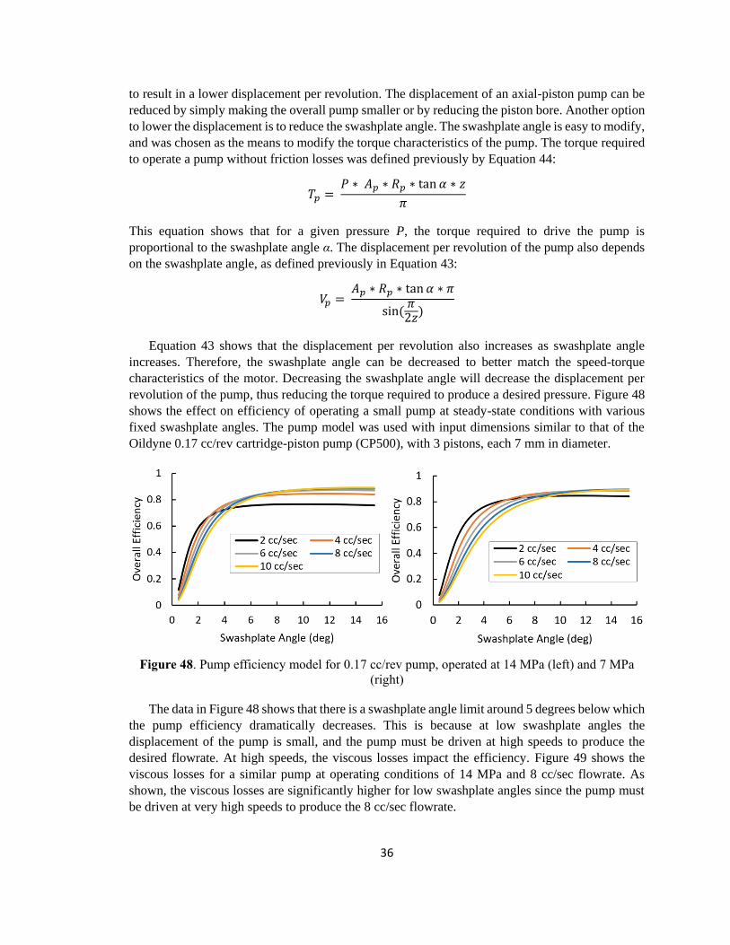
revolution of the pump, thus reducing the torque required to produce a desired pressure. Figure 48

shows the effect on efficiency of operating a small pump at steady-state conditions with various

fixed swashplate angles. The pump model was used with input dimensions similar to that of the

Oildyne 0.17 cc/rev cartridge-piston pump (CP500), with 3 pistons, each 7 mm in diameter.

Figure 48. Pump efficiency model for 0.17 cc/rev pump, operated at 14 MPa (left) and 7 MPa

(right)

The data in Figure 48 shows that there is a swashplate angle limit around 5 degrees below which

the pump efficiency dramatically decreases. This is because at low swashplate angles the

displacement of the pump is small, and the pump must be driven at high speeds to produce the

desired flowrate. At high speeds, the viscous losses impact the efficiency. Figure 49 shows the

viscous losses for a similar pump at operating conditions of 14 MPa and 8 cc/sec flowrate. As

shown, the viscous losses are significantly higher for low swashplate angles since the pump must

be driven at very high speeds to produce the 8 cc/sec flowrate.

37

Figure 49. Breakdown of torque losses in 0.17 cc/rev axial-piston pump operated at 14 MPa, 8

cc/sec, torque loss is difference in required torque to drive pump versus required torque with no

friction losses

A reduction in the piston diameter would accomplish the same task as reducing the swashplate

angle. Referring to Equations 43-44, a piston diameter reduction would decrease the torque and

decrease the flowrate per revolution of the pump. As with the swashplate angle decrease, a piston

diameter decrease would require the pump to be driven at a higher speed to produce a certain

flowrate. A similar trend occurs with viscous losses beginning to dominate as smaller and smaller

piston diameters are used. This trend is seen with all types of pumps, regardless of geometry,

because as the pump displacement per revolution is decreased to reduce torque requirements, the

pump must be driven at higher speeds, resulting in increased viscous losses.

If the swashplate angle of a small axial-piston pump is reduced to around 5 degrees to better

match the speed-torque characteristics of an electric motor, it is necessary to determine what range

of torques are required by the electric motor for various operating pressures.

Figure 50. Motor torque to drive pump (left), maximum continuous motor

torque for various motor sizes (right)

38

The left plot in Figure 50 shows that for a 3-piston, 7 mm piston diameter pump, the torque

required to output 14 MPa is in the range of 0.4-0.6 Nm for swashplate angles in the range of 5-8

deg. Shown by the plot on the right, motors above 150 W could produce this torque. Therefore, a

gearbox could be eliminated and the electric motor could be directly coupled to the pump, thus

eliminating both the added weight of the gearbox itself as well as the added weight of the battery

due to the inefficiencies of the gearbox, which would often be below 80%.

Another aspect to consider is that a gearbox can allow a motor to operate more efficiently, which

would reduce the battery weight. Figure 51 shows a case that uses a fixed 150 W size motor driving

a fixed 0.17 cc/rev axial-piston pump for a 2 hour runtime at 10 cc/sec. The overall system weight

was calculated for various gear reduction ratios applied to the motor-pump connection for pressures

of 5 and 15 MPa.

Figure 51. Gear reduction exploration effect on system weight, 5 MPa (left), 15

MPa (right), assuming ideal gearbox with no weight or efficiency losses

For lower pressures, adding a gear reduction does not lower the overall system weight.

However, as shown in Figure 51, at higher pressures a gear reduction ratio allows the fixed motor

to operate at a higher efficiency, thus resulting in a lower battery weight and a lower overall system

weight.

A gearbox configuration was considered for 9 different operating pressures and flowrates. The

weight reductions, shown in Table 5, are equivalent to the amount of battery weight saved due to

the optimized gear reduction allowing the motor to operate more efficiently.

Table 5. Optimized gearbox battery weight savings for various operating conditions,

assuming ideal, massless gearbox, 2 hr runtime, 0.17 cc/rev pump, 150 W motor

39

Table 5 shows that only the high pressure, 15 MPa cases benefited from the addition of a gear

reduction to allow the motor to operate more efficiently, thus lowering the battery weight. However,

this analysis did not consider the weight or the efficiency of the gearbox, which would result in

additional battery weight. A small gearbox may be around 150 g itself. For the three 15 MPa cases,

if the gearbox operated at an 80% efficiency, it would add 307, 617, and 968 g of battery weight to

the 5, 10, and 15 cc/sec cases, thus outweighing the reduction in battery weight due to the increase

in motor efficiency. This demonstrates that a gearbox will ultimately add additional weight to the

system

3.2.3 Motor Cooling

Another weight reduction method that was explored was the idea of using active cooling

systems to allow the use of a smaller, lighter motor. The primary limit on maximum motor power

operation is ensuring that overheating does not occur. With active cooling, a smaller motor can be

used without overheating. Figure 52 shows the maximum power rating for a range of motor sizes

in several cooling conditions. As the cooling convection coefficient is increased the maximum

continuous power a motor can operate at also increases.

Figure 52: Active cooling effect on maximum motor power rating for various

convection cooling coefficients, results from thermal motor model

While a smaller motor would reduce motor weight, there are several tradeoffs that must be

considered. As demonstrated by the motor sizing exploration, although a smaller motor is lighter,

it is often less efficient than a larger motor, thus resulting in more battery weight. This tradeoff was

explored for various operating conditions to assess the potential weight savings. Figure 53 shows

the motor size that results in a minimal system weight for various system runtimes. This was done

for the same conditions as shown in Figure 47, where a fixed 0.17 cc/rev pump was used and

operation conditions of 5 MPa and 5 cc/sec were specified. This study demonstrated that the motor

size required to produce a minimum system weight for the given conditions was 62 W and 100 W

for runtimes of 0.5 and 8 hours. Figure 53 below shows the motor size that results in a minimum

system weight for a range of desired run times, with all other setup conditions held constant.

40

Figure 53. Optimal motor size selection is dependent on runtime,

5 MPa, 5 cc/sec, weight of active cooling systems not considered

This shows that as the desired runtime is increased, the motor size that results in a minimum

system weight also increases. This is because at longer runtimes, the battery weight dominates

overall system weight, so using a heavier, more efficient motor is optimal for minimizing system

weight. Using the motor model, it was determined that the minimum possible motor size that could

drive the pump at continuous conditions of 5 MPa and 5 cc/sec was 81 W to ensure overheating

did not occur. This means that for the runtimes under 2.5 hours, where the optimally-sized motor

is below 81 W, active cooling is required to allow the motor to run without overheating. For

designed runtimes above 2.5 hours, active cooling would not be required, and oversized motors

would produce lower overall system weights.

For active cooling it is useful to determine what the approximate weight savings would be if a

cooling system was implemented to allow undersized motors to operate. Figure 54 shows the case

for a 0.5 hour runtime, showing the overall system weight using a range of motor sizes. The 46 g

difference is the total system weight difference between using active cooling to be able to use the

weight-optimum, undersized 62 W motor versus using the minimum 81 W motor without cooling.

Figure 54. 0.5 hr. runtime, system weight difference between using

41

an actively-cooled 62 W motor compared to using a non-cooled 81 W motor

This 46 g savings does not consider the weight added by the cooling system, which would likely

be more than 46 g. Additionally, several operating pressures, flowrates, and runtimes were

modelled to determine the weight savings of using undersized motors with active cooling systems

for short design runtimes. Most cases showed that using a zero-weight cooling system could reduce

overall system weight for design runtimes under about 3 hours.

Figure 55. Left: 10 MPa, 5 cc/sec, 133 W minimum motor without active cooling;

Right: 1 hr runtime, comparing ideal sized motor vs. minimum motor without active cooling

These cases resulted in weight savings in the range of 40-130 g when using an undersized motor

versus the minimum sized motor without active cooling for short runtimes around 0.5-1.0 hours

(Appendix C). Again, this analysis did not include the weight of an active cooling system. A

practical cooling system might include a small fan as well as additional battery weight needed to

power the fan. For example, a small blower fan (Fugetek 12V fan) weighs about 80 g. The power

consumption is 6 W, which for a 1 hour runtime would translate to about 40 g of battery weight.

So, adding a basic cooling system such as this may add somewhere around 120 g to the system.

Therefore, an active cooling system does not reduce overall system weight, especially for long

system runtimes.

Shown in Figure 55, as the designed runtime for a system is increased, the weight of the battery

becomes dominant in the overall system weight, and therefore larger, more efficient, electric motors

result in lower overall system weights. However, also shown in Figure 56, the energy density of

the batteries used has an impact on optimal motor selection for a minimized system weight. The

plot shows the optimal motor size for a range of design runtimes.

42

Figure 56: Effect of battery energy density on system design motor size selection

for 10 MPa, 5 cc/sec, and a 0.17 cc/rev pump

As the energy density of the battery goes down, the weight of the battery becomes an even higher

percent of the overall system weight. This means that for lower battery energy densities it is more

important to select larger motors that operate more efficiently than for cases where the battery

energy density is high.

Another area where a cooling system might potentially reduce overall weight comes from the

resistivity of copper being temperature dependent. As the motor is cooled, the resistivity of the

copper windings is reduced, making the electric motor more efficient, thus resulting in a lower

battery weight. Figure 57 demonstrates the effect of actively cooling an 80 W motor driving a 0.17

cc/rev pump at 5 MPa and various flowrates.

Figure 57. Copper winding loss effect on motor efficiency due to copper temperature dependence

The results show that the temperature difference of the windings due to using active cooling

does not have a significant impact on the overall efficiency of the motor. A maximum increase in

efficiency of about 3% was observed.

43

3.2.4 Total System Design

A combined system model was used to aid in the design of a complete minimal-weight system.

The inputs to the model were desired pressure, flowrate, and runtime. The program was designed

to iterate through several combinations of motor size, pump size, and pump swashplate angle. The

resulting output was the motor size, piston size, and swashplate angle that resulted in the lowest

overall system weight. Parameters such as the number of pistons was fixed to three. Figure 58

shows an output from the program with desired 10 MPa pressure, 10 cc/sec flowrate, 2 hour

runtime, and a 150 W motor. The program output in Figure 58 is only for a 150 W, but for the

entire analysis several similar plots were produced for varying motor sizes.

Figure 58. Weight optimization using fixed 150 W motor,

variable pump, and desired 10 cc/sec, 10 MPa, 2 hr runtime

The results for the minimal-weight configuration are a pump size with three pistons, 4 mm in

diameter, a 19⁰ swashplate angle, and 0.11 cc/rev displacement, a 93 W motor, and overall system

weight of 2.01 kg. As shown by Figure 58, near the lower left corner of the plot, the pump

displacement is low, with both small pistons as well as low swashplate angles. As shown in Figure

48, as the displacement of the pump is reduced to small values, viscous losses become large,

resulting in high systems weight. This combined system model could be used in the design of power

supply with a range of desired flowrates, pressures, and runtimes defined by the user.

While the total system model outputs a combination of pump and motor parameters that results

in a minimal system weight, Figure 58 shows that there is a wide range of pump parameters close

to the optimal solution that results in a system weight close to the optimal design weight. Therefore,

the combined system model could be used to either design a minimal-weight system with custom

parts or it could be used to aid in the selection of commercially available components that are close

to the optimal components determined by the model.

3.2.5 Quasi-Steady-State Model

The previously described analyses were limited steady-state operating conditions for fixed

operating pressures and flowrates. However, in a real-world application it is likely that the

operating conditions would vary throughout a cycle. The model was adapted to calculate system

44

weight for a sequence of operating pressures and flowrates. To demonstrate this, Figure 59 shows

a 9 seconds cyclical operation with three steady-state operating conditions. This analysis still does

not account for dynamic motor and pump operations, but the steady-state analysis should be

adequate for cycles with relatively low dynamic shifting. These pressures and flowrates were

chosen to be in a similar range to that of the hydraulic-ankle foot orthosis requirements.

Figure 59. Quasi-steady-state, cyclical operation

The model was used to determine the overall system weight for various motor powers and

swashplate angles for a run time of 4.5 hours (1800 cycles).

Figure 60. Quasi-steady-state system analysis results

A swashplate angle of 7.2⁰ and a motor size of 108 W results in the lowest system weight, 1.95

kg, for this set of operating conditions. Other applications that require a cyclical mode of operation

could be broken into even smaller sections for analysis. However, this method of analysis has

limitations since it does not account for dynamic operation, which may be significant for

applications with high levels of variability in operation pressure and flowrate.

45

4. Discussion and Conclusion

4.1 Test Stand Validation Discussion

4.1.1 Experimental vs. Model Predictions

The test stand results showed somewhat higher overall system weights than the simulation

predictions. As discussed, the likely reason for this mismatch was due to inefficiencies that were

unaccounted for in the simulation. After the 35% additional inefficiencies were added to the model,

the simulation results matched well to the experimental results.

4.1.2 Purpose of Model as a Tool

The purpose of this computational model is for it to be used as a tool for finding approximate

combinations of component parameters that will result in a low system weight. As shown by the

plots of the experimental results, the minimal-weight combination of motor and pump size is

usually surrounded by a relatively large area of low system weight combinations, only a small

amount higher than the minimum. Therefore, the simulation can be used to find an approximate

combination of pump and motor size that will result in a low system weight, and it is not critical to

have an exact motor and pump size combination to result in a low system weight. This simulation

tool is especially useful for avoiding combinations of pump and motor size that results in an

exceptionally high system weight. As shown by the plots in Figures 37-44, there are certain regions

of the plots that result in exceptionally high system weights. For example, Figure 38 with the 3.5

MPa, 10 cc/sec, and 8 hr runtime shows that the 5.23⁰ and 7.76⁰ pump sizes should be avoided for

all motor combinations, and the 10.05⁰ pump would result in a low system weight for all

combinations of motor sizes, especially the 100 and 180 W motors. The simulation versus the

experimental results showed that while the areas of minimum system weight generally matched,

there were some discrepancies. However, the areas of exceptionally high system weight seemed to

be a very close match for every pressure, flowrate, and runtime tested. This shows that the model

is especially useful for avoiding these poor designs.

4.1.3 HAFO Power Supply Redesign

The validated model can be used for applications such as redesigning the power supply for the

hydraulic ankle-foot orthosis. The HAFO power supply consisted of a 3.7 transmission ratio

gearbox. The HAFO power supply used a Takako 0.4 cc/rev pump with a swashplate angle of 13.2

degrees, and the original 627g battery was calculated to allow the system to run for 45 minutes at

steady-state conditions of 3.97 MPa and 10.3 cc/sec, which was calculated by finding the average

pressure and flowrate requirements for one walking cycle. The plots in Figure 62 show the minimal-

weight designs for a 45 and 120 minute runtime.

46

Figure 61. Hydraulic ankle-foot orthosis power supply

Figure 62. HAFO power supply design using computation model to explore design parameters of

motor size and pump swashplate angle

For the 45 minute runtime, a 8.0 degree swashplate angle and a 51 W motor results in the

lowest system weight. For the 120 minute runtime, a 9.9 degree swashplate angle and a 67 W

motor results in the lowest system weight. Table 6 below shows the weight comparison between

the model design and the original HAFO power supply.

Table 6. Weight comparison of original HAFO power supply to computational model design

These results show that for the 45 minute runtime, the original power supply is 192 g heavier,

and for the 120 minute runtime the original power supply is 498 g heavier. This shows that the

original power supply design is sufficient for a 45 minute runtime. However, this original design

47

performs poorly for longer runtimes, as with the 120 runtime case. For the 120 minute runtime it

would be beneficial to reduce the pump swashplate angle from 13.2 to 8.0 degrees, and use a 51 W

motor directly driving the pump.

4.2 System Design Guidelines Discussion

4.2.1 Design Guidelines

There are four main guidelines that were developed after analyzing the results of section 4.2 -

Design Guideline Development:

1. The smallest electric motor that can provide the required torque and speed may not result

in minimum system weight.

As shown previously, it is often best to select an oversized motor. As shown in Figure 46, larger

electric motors generally operate more efficiently than smaller motors, especially at high torques.

The reason is because the majority of DC electric motor losses come from winding I2R losses [20].

This can be shown by examining the equations that govern torque production in an electric motor,

𝑇 = 𝑘𝑡 ∗ 𝐼 (64)

𝐹 = 𝐼𝐿 𝑥 𝐵 (65)

𝑅 =

𝜌𝐿

𝐴 (66)

𝑃𝑤 = 𝐼2𝑅

(67)

To see how these equations demonstrate the described trend, assume two motors, one smaller

with winding length L, and one larger motor with winding length 2L. Both have equivalent wire

diameters and identical magnetic field strength B. To produce an equivalent force with both motors,

from Equation 65, the larger motor will need half the current since it has twice the length of wire.

From Equation 66, the resistance of the winding for the larger motor will be twice that of the

smaller. Then, using Equation 67 for the larger motor, the power loss will be half of the smaller

motor. Although the resistance is twice that of the smaller motor, the current is half that of the

smaller motor, thus resulting in half the power loss. Although this analysis does not consider

viscous losses, it demonstrates why larger motors operate more efficiently, especially at higher

torques.

Also, it was shown that the optimal motor size is dependent on design runtime, and as the design

runtime increases the optimal motor size also increases. This is because as the desired runtime of

the system becomes longer, the weight of the battery dominates the overall system weight. Thus,

the operating efficiency of the motor becomes more important than the weight of the motor itself.

These case studies demonstrate that it is often best to select an oversized motor, since larger

motors often operate more efficiently, which reduces battery weight and therefore overall system

weight. Also, selecting larger motors helps to ensure that overheating will not occur in the case of

unforeseen heating conditions in real-world applications.

48

2. The gearbox between the electric motor and pump should be eliminated to reduce system

weight.

As demonstrated by the case study shown in Table 5, the addition of a gearbox could allow the

motor to operate more efficiently and save battery weight in this manner. However, when

considering the additional weight added by both the gearbox itself and the additional battery weight

due to the gearbox inefficiencies, it was determined that adding a gearbox would ultimately add

weight to the system.

To directly drive the pump with an electric motor, the pump needs have sufficiently low

displacements. For motors in the 100-300 W range, the displacement of the pump must be around

0.2 cc/rev or lower to allow pressures up to 14 MPa to be generated There are very few

commercially available axial-piston pumps with such a small displacement. So, it would be

beneficial to develop designs for new pumps with even lower displacements than current available

pumps. This would allow for these motors to be directly coupled to the pumps, thus eliminating the

additional weight associated with a gearbox.

To best match the motor to the pump in a direct-drive configuration, another area to consider is

varying the motor construction. The motor model that was developed is the most common type of

BLDC motor design with an internal rotor. However, there is a less common design known as an

outer rotor design, where the windings are fixed in the center of the motor and the rotor with the

permanent magnets attached is external to this.

Figure 63. Outer and inner rotor BLDC motor designs

As shown in Figure 63 above, the radius of the acting force for the outer rotor design is greater

than for the inner rotor. This allows the outer rotor design to be able to produce higher torques at

lower speeds than the inner rotor design. This essentially creates the same effect as a gearbox by

reducing the speed and increasing the torque, which allows for a better matching of motor to pump

performance. Although these types of motors may be better suited to an application for small

hydraulic power supplies, the availability of these types of motors is limited compared to

conventional designs.

49

3. Active cooling of the motor does not reduce system weight.

Active cooling can allow undersized motors to be used for a certain application, which reduces

the motor weight in the system. However, it was shown that for several designs, this did not reduce

system weight. Using an undersized motor actually increased the overall system weight in many

cases. This is again due to the fact that larger motors often operate more efficiently. Although an

undersized motor may reduce the motor weight, because the smaller motor if less efficient, it will

add additional battery weight to the system. Therefore, active cooling should not be used in an

attempt to reduce overall system weight. However, in real-world applications of such power

supplies, cooling systems may still be of potential use to ensure that the motor does not overheat in

the case of variations in natural convection cooling conditions. Also, for systems designed for very

short runtimes under 30 minutes, it may be effective to use active cooling and an undersized motor

since the battery weight is not a significant amount of the overall system weight at these runtimes,

and it is therefore not as important to use a more efficient, heavier motor.

4. Iterative modeling is necessary to determine the various range of component parameters

necessary to result in a minimal-weight system

As shown by the analyses performed in this study, there are several factors that contribute to

the selection of individual components. Additionally, the selection of one component influences

the operational efficiency of the other components in the system. Therefore, while it is useful to

have basic guidelines to aid in the selection of components, the best was to design a system is to

use the computational model to iterate through a wide range of design possibilities.

4.2.2 Limitations of Guidelines

The system design guidelines can be used aid in the design of a lightweight hydraulic power

supply. One limitation of these guidelines is that the analyses for this project were all done for

steady-state operation. While the quasi-steady-state model addressed this matter, the quasi-steady-

state model assumes that dynamic operating effects are negligible. For systems that have a high

degree of dynamic changes in pressure and flowrate requirements throughout a cycle, it may be the

case that the models developed would not be accurate. Therefore, the model developed should be

used for systems that have low levels of dynamic changes in pressure and flowrate.

Although the steady-state limitation on the models may not translate perfectly to a dynamically

changing system, many of the design guidelines would likely still apply. For example, even with

dynamic changes in motor speed and direction, the fact that larger motors will generally operate

more efficiently than small motors still applies, and therefore the guideline are a good place to start

when designing small-scale power supplies.

50

5. References

[1] Akers, A., Gassman, M., and Smith, R., Hydraulic Power System Analysis. Taylor &

Francis, 2006.

[2] Durfee, W., and Sun, Z., Fluid Power System Dynamics. Center for Compact and

Efficient Fluid Power, 2009.

[3] Hunt, T.M., The Hydraulic Handbook. Elsevier, 1996.

[4] Gilbertson, M., Beekman, D., Mohanty, B., Hashemi, S., Lee, S., Van de Ven, J. D., &

Kowalewski, T. M. (2016, October). Force Analysis and Modelling of Soft Actuators for

Catheter Robots. In ASME 2016 Dynamic Systems and Control Conference (pp.

V002T25A005-V002T25A005). American Society of Mechanical Engineers of Physical

Medicine & Rehabilitation, 71(2), pp. 112-115.

[5] Shields, Guy; Kovalsky, Corrine (27 September 2010). "Raytheon Unveils Lighter,

Faster, Stronger Second Generation Exoskeleton Robotic Suit". Raytheon. Retrieved 9

July 2016.

[6] (June 2011) “Lockheed Martin’s HULC Robotic Exoskeleton Enters Biomechanical

Testing at U.S. Army Natick Soldier Systems Center” available at: lockheedmartin.com,

Retrieved 10 October 2016

[7] www.bostondynamics.com/bigdog, 2017 Boston Dynamics

[8]

www.bostondynamics.com/spot, 2017 Boston Dynamics

[9] National Research Council. 2004. Meeting the Energy Needs of Future Warriors.

Washington, DC: The National Academies Press. doi:https://doi.org/10.17226/11065.

[10] Jicheng, Xia, 2015, “Modeling and Analysis of Small-Scale Hydraulic Systems” PhD.

Thesis, University of Minnesota, Minneapolis, MN

[11] Neubauer, Brett, 2017, “Principles of Small-Scale Hydraulic Systems for Human-

Assistive Machines” PhD Thesis, University of Minnesota, Minneapolis

[12] “New Quadruped Robot Takes Big Strides Toward Saving Lives” Moog Industrial

Newsletter Issue 38, October 2015

[13] Neubauer, B., Nath, J., and Durfee, W., 2014. “Design of a portable hydraulic ankle-foot

orthosis”. In Engineering in Medicine and Biology Society (EMBC), 2014 36th Annual

51

International Conference of the IEEE. IEEE, 2014, pp. 1182–1185.

[14] Rahn, Christopher D. Battery Systems Engineering. Hoboken: Wiley, 2013.

[15] Toliyat, Hamid A., and Gerald B. Kliman, eds. Handbook of electric motors. Vol. 120.

CRC press, 2004

[16] Yedamale P., Microchip Technology In., “Brushless DC (BLDC) Motor Fundamentals”

AN885

[17] Wilson, W. E., 1950. Positive-displacement pumps and fluid motors. Pitman, London.

[18] Metallic Materials Specification Handbook, Fourth Ed., Robert B. Ross, Chapman &

Hall, London, 1992

[19] Juha Pyrhönen; Tapani Jokinen; Valéria Hrabovcová (2009). Design of Rotating

Electrical Machines. John Wiley and Sons. p. 232. ISBN 0-470-69516-1.

[20] Tong, Wei., Mechanical Design of Electric Motors. CRC press, 2014

[21] Bergman, T., Lavine, A., Incropera, F., DeWitt, D., Fundamentals of Heat and Mass

Transfer 7th Edition, John Wiley and Sons, April 2011

[22] Jeong, H., 2007. “A novel performance model given by the physical dimensions of

hydraulic axial piston motors: model derivation”. Journal of Mechanical Science and

Technology, 21(1), pp. 83–97.

[23] Xia, J., & Durfee, W. K., 2014. Experimentally validated Models of O-ring seals for tiny

hydraulic cylinders. In ASME/BATH 2014 Symposium on Fluid Power and Motion

Control, FPMC 2014 Web Portal ASME (American Society Of Mechanical Engineers).

DOI: 10.1115/FPMC2014-7825

[24] Hashemi, S., & Durfee, W., 2017. Low-Friction, Long- Stroke Rolling Diaphragm

Cylinder for Passive Hydraulic Rehabilitation Robots. In press, ASME Journal of Medical Devices

52

Appendix

A: Pump Dimensions

The distance between the ball joint on the piston and the top of the cylinder block while the piston

is at bottom dead center is as follows:

𝑙𝐵𝑂 = 𝑅𝑝 ∗ tan 𝛼

This displacement per piston can also be defined as follows:

𝑉𝑃𝑚𝑎𝑥 = 𝐴𝑝 ∗ (𝑙𝑝 − 𝑙𝐵𝑂 − 𝑙𝐹)

The length of the piston inside of the cylinder block at top dead center is as follows:

𝑙𝐹 = 𝑙𝑝 − 𝑙𝐵𝑂 − 𝜋 ∗ 𝑅𝑝 ∗ tan 𝛼

sin (𝜋2𝑧

)

The length that the piston travels from top dead center to bottom dead center is:

𝑙𝐶𝑂 = 𝑙𝑝 − 𝑙𝐹 − 𝑙𝐵𝑂

The radius of the slipper pad is estimated to be as follows:

𝑟𝑠𝑜 =5

4∗ 𝑑𝑝

The diagram below shows the key dimensions of the valve plate.

53

Figure 57: Key valve plate dimensions

The following equations can be used to approximate the valve plate dimensions:

𝜆𝑣 = 0.4 ∗ 𝑑𝑝

𝑏𝑣1 = 0.15 ∗ 𝑑𝑝

𝑏𝑣1 = 𝑏𝑣2

𝑙𝑣 = 𝑏𝑣1 ∗ 𝑏𝑣2

𝑏𝑣1 + 𝑏𝑣2

𝑠 = 2 ∗ [𝑅𝑝 ∗ sin (180

𝑧) −

𝑑𝑝

2]

𝑟𝑣4 = 𝑅𝑝 + 𝑠 +𝑑𝑝

2

𝑟𝑣1 = 𝑅𝑝 − 𝑠 −𝑑𝑝

2

𝑟𝑣3 = 𝑟𝑣4 − 𝑏𝑣2

𝑟𝑣2 = 𝑟𝑣1 − 𝑏𝑣1

B: Takako Pump Dimensions

54

C: Motor Cooling

55

D: Test Stand Data

OPTIMIZATION AND DESIGN PRINCIPLES OF A MINIMAL …

Documents

Transcript of OPTIMIZATION AND DESIGN PRINCIPLES OF A MINIMAL …