Optimal Feedback Law Recovery by Gradient-Augmented Sparse ...

Journal of Machine Learning Research 22 (2021) 1-32 Submitted 7/20; Revised 11/20; Published 1/21

Optimal Feedback Law Recovery by Gradient-AugmentedSparse Polynomial Regression

Behzad Azmi [email protected] Institute for Computational and Applied MathematicsAustrian Academy of SciencesAltenbergerstraße 69, A-4040 Linz, Austria

Dante Kalise [email protected] of Mathematical SciencesUniversity of NottinghamUniversity Park, Nottingham NG7 2QL, United Kingdom

Karl Kunisch [email protected]

Radon Institute for Computational and Applied Mathematics

Austrian Academy of Sciences

and

Institute of Mathematics and Scientific Computing

University of Graz

Heinrichstraße 36, A-8010 Graz, Austria

Editor: George Konidaris

Abstract

A sparse regression approach for the computation of high-dimensional optimal feedback laws aris-ing in deterministic nonlinear control is proposed. The approach exploits the control-theoreticallink between Hamilton-Jacobi-Bellman PDEs characterizing the value function of the optimalcontrol problems, and first-order optimality conditions via Pontryagin’s Maximum Principle.The latter is used as a representation formula to recover the value function and its gradient atarbitrary points in the space-time domain through the solution of a two-point boundary valueproblem. After generating a dataset consisting of different state-value pairs, a hyperbolic crosspolynomial model for the value function is fitted using a LASSO regression. An extended set oflow and high-dimensional numerical tests in nonlinear optimal control reveal that enriching thedataset with gradient information reduces the number of training samples, and that the sparsepolynomial regression consistently yields a feedback law of lower complexity.

Keywords: Optimal Feedback Control, Optimality Conditions, Hamilton-Jacobi-BellmanPDE, Polynomial Approximation, Sparse Optimization

1. Introduction

A large class of design problems including the synthesis of autopilot and guidance systems, thestabilization of chemical reactions, and the control of fluid flow phenomena, among others, canbe cast as deterministic nonlinear optimal control problems. In this framework, we synthesize atime-dependent control signal u(t) in Rm by solving a dynamic optimization problem which we

c©2021 Behzad Azmi, Dante Kalise, and Karl Kunisch.

License: CC-BY 4.0, see https://creativecommons.org/licenses/by/4.0/. Attribution requirements are provided athttp://jmlr.org/papers/v22/20-755.html.

https://creativecommons.org/licenses/by/4.0/

http://jmlr.org/papers/v22/20-755.html

Azmi, Kalise and Kunisch

formulate as

minu(·)∈L2(t0,T ;Rm)

J(u; t0,x) :=

∫ >t0

`(y(t)) + β‖u(t))‖22 dt , β > 0 , (1)

subject to y(t) in Rn being the solution to the control-affine nonlinear dynamics

d

dty(t) = f(y(t)) + g(y(t))u(t) , y(t0) = x . (2)

We assume that the running cost ` : Rn → R, the dynamics f : Rn → Rn, and g : Rn → Rn×m,are continuously differentiable. The numerical realization of control laws by solving the dynamicoptimization problem above is a topic at the interface between control theory, computationaloptimization, and numerical analysis. While this problem dates back to the birth of Calculusof Variations, it was during the second half of the 20th century when two major methodologicalbreakthroughs shaped our understanding of optimal control theory, namely, the developmentof Pontryagin’s Maximum Principle and the theory of Dynamic Programming (see (Pesch andPlail, 2009) for a historical survey on this topic). On the one hand, Pontryagin’s MaximumPrinciple (PMP) (Pontryagin et al., 1962) yields first-order optimality conditions for (1)-(2)in the form of a two-point boundary value problem for a forward-backward coupling betweenoptimal state,adjoint p∗ = (p∗1, . . . , p

∗n), and control variables, denoted by (y∗(t),p∗(t),u∗(t))

respectively, which in short reads

d

dty∗(t) = f(y∗(t)) + g(y∗(t))u∗(t) ,

y∗(t0) = x ,

− d

dtp∗(t) = ∂y(f(y∗(t)) + g(y∗(t))u∗(t))>p(t) + ∂y`(y

∗(t)) ,

p∗(T ) = 0 ,

(TPBVP)

closed with the optimality condition

u∗(t) = − 1

2βg>(y∗(t))p∗(t) , ∀t ∈ (t0, T ) . (3)

This procedure yields an optimal state-adjoint-control triple originating from the initial conditionx, in what is known as an open-loop control. On the other hand, the Dynamic Programmingapproach synthesizes the optimal control as

u∗(t,x) = argminu∈Rm

β‖u‖22 +∇V (t,x)> (g(x)u)

= − 1

2βg>(x)∇V (t,x) , (4)

where V (t,x) : [0, T ]× Rn −→ R is the value function of the problem

V (t,x) := infu(·)J(u; t,x) subject to (2) , (5)

which in turn satisfies a first-order, nonlinear Hamilton-Jacobi-Bellman (HJB) partial differentialequation of the form

∂tV (t,x)− 12β∇V (t,x)>g(x)g>(x)∇V (t,x) +∇V (t,x)>f(x) + `(x) = 0 ,

V (T,x) = 0 ,(HJB)

2

Optimal Feedback Law Recovery by Gradient-Augmented Polynomial Regression

to be solved over the state space of the dynamics X ⊂ Rn (Bardi and Capuzzo-Dolcetta, 1997,Chapter 1). Here and throughout we assume that V is C1, see e.g.Frankowska (2002). This ap-proach expresses the optimal control as a feedback map or closed-loop form, i.e. u∗ = u∗(t,y(t)),yielding a control law that is optimal in the whole state space. From a practical viewpoint,optimal trajectories obtained from the solution of (TPBVP) are not robust with respect to dis-turbances, justifying the necessity of a HJB-based feedback synthesis. However, the solution ofHJB PDEs, especially for high-dimensional dynamical systems, comes at a formidable computa-tional cost, often referred in the literature as the curse of dimensionality (Bellman, 1961). Overthe last years, a number of works have reported remarkable progress in the solution of high-dimensional HJB PDEs, including the use of sparse grids (Garcke and Kroner, 2017; Bokanowskiet al., 2013), tree structure algorithms (Alla et al., 2019), max-plus methods (McEneaney, 2007;Akian et al., 2008), polynomial approximation (Kalise et al., 2020; Kalise and Kunisch, 2018),tensor decomposition techniques (Horowitz et al., 2014; Stefansson and Leong, 2016; Gorodetskyet al., 2018; Dolgov et al., 2019; Oster et al., 2019), and an evergrowing literature on artificialneural networks (Han et al., 2018; Darbon et al., 2020; Nusken and Richter, 2020; Ito et al.,2020; Kunisch and Walter, 2020).

On the link between PMP and HJB PDEs. In this work, we follow an alternative ap-proach that circumvents the curse of dimensionality in the computation of optimal feedback lawsby exploiting the relation between the HJB PDE and the PMP. We interpret system (TPBVP)as a representation formula for the solution of (HJB) . There exists an extensive literaturedating back to (Pontryagin et al., 1962, Chapter 1) discussing the relation between dynamicprogramming and first-order optimality conditions. In the simplest version of the statement,assuming the solution of the HJB PDE is C2, it can be shown that the forward-backward dynam-ics originating from the PMP correspond to the characteristic curves of the HJB equation.Thisresult was further improved in (Barron and Jensen, 1986), where the PMP was derived from theviscosity solution of a first-order HJB PDE. The precise result linking the solution of the PMPwith the characteristic curves of the HJB PDE, and the identification of the adjoint variable asthe gradient of the value function can be found in (Subbotina, 2004, Theorems II.9 and II.10).We refer the reader to (Bardi and Capuzzo-Dolcetta, 1997, Section 3.4) for an exhaustive revi-sion of the main results in this topic. More concretely, the computation of a given V (ti,xi) canbe realized by solving (TPBVP) setting t0 = ti and the initial condition y(t0) = xi, and evalu-ating the optimal cost (1) using the optimal triple (y∗(t),p∗(t),u∗(t)). Moreover, the optimaladjoint verifies p∗(t) = ∇V (t,y∗(t)) (Clarke and Vinter, 1987; Cannarsa and Frankowska, 1991;Cristiani and Martinon, 2010). The PMP can be thus understood as a representation formulafor the value function and its gradient along an optimal trajectory.

A data-driven method for computing optimal feedback laws. We restrict our atten-tion to a class of smooth and unconstrained nonlinear optimal control problems where theaforedescribed link between PMP and the HJB PDE is direct, and we use it to generate acharacteristic-based, causality-free method to approximate V (t,x) and as a by-product u(t,x),without solving (HJB). To do this, we sample a set of initial conditions (ti,xi)Ni=1, for whichwe compute both V (ti,xi) and ∇V (ti,xi) by realizing the optimal trajectory through PMP.This is done by following a reduced gradient approach (Herzog and Kunisch, 2010), in whichforward-backward iterative solves of (TPBVP) are combined with a gradient descent methodto find the minimizer of J(u; t0,x). Having collected a dataset ti,xi, V (ti,xi),∇V (ti,xi)Ni=1

3


enriched with gradient information, we fit a polynomial model for the value function

Vθ(t,x) =

q∑i=1

θiΦi(t,x) = 〈θ,Φ〉 , (6)

with Φ(t,x) = (Φ1(t,x), . . . ,Φq(t,x)) are elements of a suitable polynomial basis, and the pa-rameters θ = (θ1, . . . , θq) obtained from a LASSO regression

minθ∈Rq‖[Φ;∇Φ] θ − [V ;∇V ]‖22 + λ‖θ‖1,w , (7)

where the matrix [Φ;∇Φ] ∈ R(n+1)N×q and the vector [V ;∇V ] ∈ R(n+1)N include value functionand gradient data. Finally, the optimal feedback map is recovered as

u∗(t,x) = argminu

β‖u‖22 +∇Vθ(t,x)> (g(x)u) . (8)

Recall from the discussion above that the gradient ∇V (x) can be obtained at no extra cost fromopen-loop evaluations of V (x).

Related literature and contributions. The idea of using open-loop solves to build a nu-merical representation of an optimal feedback law dates back at least to (Beeler et al., 2000;Ito and Schroeter, 2001), where a low-dimensional feedback law was constructed directly byinterpolating the optimal control from a set of collocation points. More recently, this idea hasbeen revisited and improved in (Kang and Wilcox, 2017, 2015) by exploiting the extremelyparallelizable structure of the open-loop solves together with a sparse grid interpolant, scalingup to 6-dimensional examples. In (Nakamura-Zimmerer et al., 2019; Kang et al., 2019) this ideahas been further developed by replacing the use of a grid-based interpolant with artificial neuralnetworks which are trained using a dataset consisting of both the value function and gradientevaluations, presenting computational results up to dimension 30. In a similar vein, the works(Chow et al., 2019, 2018, 2017; Darbon and Osher, 2016) have proposed the use of representationformulas for HJB PDEs, ranging from the celebrated Lax-Hopf formula to variations of the PMP,in conjunction with efficient convex optimization techniques for the solution of point values ofthe HJB PDE on the fly. These results have been further studied in (Yegorov and Dower, 2018),and used in (Yegorov et al., 2019; lar, 2020) for the construction of control Lyapunov functionsboth with sparse grids and neural networks. Our work, while in line with the aforedescribed,proposes a different methodology which is summarized in the following ingredients:

• An enriched dataset containing both value function and gradient information. Approxi-mating a function based on measurements of both the function values and its derivativesdates back to Hermite and spline interpolants. Here, we follow the approach presentedin (Adcock and Sui, 2019), where gradient information is used in a sparse regressionframework, showing that gradient-augmented sparse regression can reduce the amount ofsamples required to reach a certain training error. In our case, samples are obtained fromthe solution of open-loop solves that are realized through a reduced gradient approach.The reduction of the number of samples due to the inclusion of gradient information isparticularly relevant for high-dimensional nonlinear optimal control problems, as samplinggeneration can be particularly costly.

4


• The value function, and as a consequence the feedback law, is approximated with a polyno-mial ansatz (6). This choice is backed by the extensive literature concerning power seriesapproximations of the value function (Al’brekht, 1961; Krener et al., 2013; Lukes, 1969;Bre, 2019). In fact, it is well-known that for linear dynamics and quadratic cost functions,the value function corresponds to a quadratic form, which is contained in the span of ourapproximation space. In (Kalise et al., 2020; Kalise and Kunisch, 2018), we have studied aGalerkin approach for HJB PDEs arising in nonlinear control and games with polynomialapproximation functions. In these works we have constructed a polynomial basis limitedby the total degree of the monomials, solving up to 14-dimensional tests. Here instead,borrowing a leaf from the vast literature on polynomial approximation theory (Beck et al.,2012; Chkifa et al., 2015b; Cohen et al., 2011; Chkifa et al., 2015a), we consider a hierar-chical basis defined through hyperbolic cross approximation, for which we report tests upto dimension 80 at moderate computational cost. Following results such as (Adcock andSui, 2019, Theorem 4.1), the sparse regression of a feedback law with gradient-augmentedinformation and a hyperbolic cross expansion has an error in the H1-norm that is gov-erned by the projection of the original value function over the hyperbolic cross set1 Ingeneral, given an optimal control problem, it is difficult to establish a priori bounds forthis projection error. This is mainly due to the fact that the regularity of V as a functionof f, g and ` is difficult to quantify. Of course, for the linear-quadratic control problemthe value function is a quadratic function and therefore it can be accurately representedby expansion in the hyperbolic cross with low polynomial degree. Sufficient conditions forlocal C2, 1-regularity of V are given in Cannarsa and Frankowska (2013). Higher orderregularity will depend on the problem structure, see e.g. Bre (2019). As we restrict ourproblem formulation to control-affine dynamics without control or state constraint andsmooth value functions, circumventing the fully nonlinear case, we expect that the valuefunction can be correctly captured by quadratic and high-order polynomial terms.

• The use of a polynomial expansion for the value function, which is linear in the coefficients,allows us to fit the value function model through a LASSO regression framework (7). Thisleast squares problem can easily account for the use of gradient data and has a well-understood numerical realization (Adcock and Sui, 2019; Laurent et al., 2019). Moreover,we include an `1 penalty on the expansion coefficients, leading to the synthesis of lowcomplexity feedback laws (8), which is crucial for a fast online computation of the feedbackaction.

• Our extensive numerical assessment of the methodology includes a class of genuinely non-linear, fully coupled, high-dimensional dynamics arising in agent-based modelling (Choiet al., 2019), which ultimately connects with the control of non-local transport equationsarising in mean field control (Albi et al., 2017; Fornasier and Solombrino, 2014; Gomesand Pavliotis, 2018).

Stabilization with static feedback laws. For large optimization horizon T, and `(y) =‖y‖2, the cost (1) can be considered as an approximation to the asymptotic stabilization problemwere T =∞. This scenario will be the focus of our numerical tests. This also motivates that inthe rest of the paper we will restrict our presentation to the approximation of V (0,x) = V (x)and ∇V (0,x) = ∇V (x), and to the associated static feedback law u∗(0,x) = u∗(x). This

1. assuming a sufficiently large training set, which we generate offline.

5


approximation also relates to the one done in nonlinear model predictive control, where afteran open-loop solve is computed, the initial optimal control u∗(0) is used to evolve the stateequation for a short period , after which the open-loop optimization is re-computed with anupdated initial state. It can be shown that as the prediction horizon T increases, the optimalcontrol approaches the stationary feedback laws, see for instance (Azmi and Kunisch, 2016;Grune and Rantzer, 2008; Reble and Allgower, 2012; Worthmann et al., 2014). For the readerinterested in obtaining the complete time-dependent optimal feedback law, we discuss at theend of Section 2 how to extend the proposed methodology.

The rest of the paper is structured as follows. In Section 2, we describe our numericalmethodology, including the numerical generation of the dataset, the polynomial ansatz for thevalue function and the model fit through LASSO regression. Then, in Section 3 we presentan exhaustive numerical assessment of the proposed methodology, including the synthesis ofhigh-dimensional optimal feedback laws for nonlinear PDEs and multiagent systems.

2. Data-driven Recovery of Feedback Laws

In this section, we develop the different building blocks of the proposed approach. We first discusshow to generate the training dataset by solving a set of open-loop optimal control problems witha reduced gradient approach. Next, we build a polynomial model for the value function basedon a hyperbolic cross approximation. Having specified both the data and the model, we fitour model with a LASSO regression. At the end of the section, we explain how to modify theproposed framework to recover time-dependent feedback laws.

2.1 Generating a dataset with a reduced gradient approach

We begin by generating a dataset xj , V (0,xj),∇V (0,xj)Nj=1 which is obtained from solvingopen-loop optimal control problems of the form (1) (with t0 = 0 and T sufficiently large) throughthe use of first-order optimality conditions (2)-(3). For this purpose we follow a reduced gradientapproach with a Barzilai-Borwein update (Barzilai and Borwein, 1988; Azmi and Kunisch, 2020),which is summarized as follows.

Assuming that the solution operator y(u) = y(u,x) corresponding to the state equation (2) iswell-defined and continuously differentiable, we can rewrite (1)-(2) as the following unconstraineddynamic optimization problem depending solely on the control variable u

minu(·)J (u) = min

u(·)J(y(u),u) = min

(y(·),u(·))J(y,u) : subject to e(y,u) = 0, (9)

where

e(y,u) :=

(ddty(t)− (f(y(t)) + g(y(t))u(t))

y(0)− x

). (10)

Formally, we obtain the directional derivative of J at u ∈ L2(0, T ;Rm) in a direction δu ∈L2(0, T ;Rm) by computing

J ′(u)δu = (G(u), δu) = ((y′(u))∗∂yJ(v) + ∂uJ(v), δu), (11)

where v := (y, u) with y := y(u), G denotes the gradient of J , (·, ·) stands for the scalar productin the space of controls L2(0, T ;Rm), and the superscript ∗ corresponds to the adjoint operator.Moreover, the term y′(u) is given by

y′(u)δu = −(∂ye(v))−1∂ue(v)δu. (12)

6


It can be shown that (∂ye(y(u),u))−1, defined by (φ,q0) 7→ q, is the solution operator of thefollowing linearised equation

ddtq(t)− ∂y (f(y(t)) + g(y(t))u(t))q(t) = φ,

q(0) = q0,(13)

and that the adjoint operator (∂ye(y(u),u))−∗ defined by (ψ,pT ) 7→ p, is the solution operatorto the following backward-in-time equation

− ddtp(t)− (∂y (f(y(t)) + g(y(t))u(t))> p(t) = ψ,

p(T ) = pT .(14)

Putting these elements together, we are now in a position to compute the gradient G of J at u.Using (11) and (12), we obtain

G(u) = ∂uJ(v)− (∂ue(v))∗(∂ye(v))−∗∂yJ(v) , (15)

and therefore, for almost every t ∈ (0, T ), we have

G(u)(t) = g(y(t))>p(t) + 2βu(t), (16)

where p is the solution to− ddtp(t)− (∂y (f(y(t)) + g(y(t))u(t))> p(t) = ∂y`(y(t)),

p(T ) = 0.(17)

Having a realization of the reduced gradient, we follow the Barzilai-Borwein gradient methodfor finding the stationary point u∗ of J ( i.e. G(u∗) = 0). In this method, the stepsizes arechosen according to be either

αBB1k :=

(Sk−1,Yk−1)

(Sk−1,Sk−1), or αBB2

k :=(Yk−1,Yk−1)

(Sk−1,Yk−1), (18)

where Gk := G(uk), Sk−1 := uk − uk−1 and Yk−1 := Gk − Gk−1. With these specifications, weintroduce Algorithm 1, which is used for solving the open-loop problems. Note that the formulasabove are written for continuous-time dynamical systems. In practice, Algorithm 1 is expectedto be used in conjunction with a suitable numerical integrator for an accurate approximationof both the state and its adjoint. Finally, fixing an initial condition xj , after Algorithm 1 hasconverged to u∗ the dataset is completed with V (xj) = J (u∗) and ∇V (xj) = p∗(0).

2.2 Building a polynomial model for the value function

Having generated a dataset for recovering the value function associated to the optimal controlproblem, we now turn our attention to deriving a suitable model for regression. Our approxi-mation of the static value function V (x) : Rn → R follows the ideas presented in (Adcock andSui, 2019; Adcock et al., 2019).

Let D ⊂ Rn be a bounded domain and Φii∈Nn0 be a tensor-product orthonormal basisof L2(D). We consider bases which are polynomial, using for instance Legendre or Chebyshev

7


Algorithm 1 Barzilai-Borwein two-point step-size gradient method

Input: Choose u−1 := 0 and u0 := −G(0), tolerance tol > 0.1: Set k = 0.2: while ‖Gk‖ ≥ tol , do3: Compute yk(uk) via (2).4: Compute pk(yk,uk) via (17).5: Compute Gk = G(uk) using (16) with (yk,pk,uk).6: Choose

αk =

αBB1k for odd k,

αBB2k for even k.

7: Set dk = 1αkGk.

8: Compute the step-size ηk > 0 based on the non-monotone linesearch given in (Dai andZhang, 2001).

9: Set uk+1 = uk − ηkdk, k = k + 1, and go to Step 2.

polynomials. Concretely, assume that D := (−1, 1)n and that φi∞i=0 is one-dimensional or-thonormal basis of L2(−1, 1). Then, the corresponding tensor-product basis of L2(D) is definedby

Φi(x) :=n∏j=1

φij (xi) , with i = (i1, i2, . . . , in) ∈ Nn, x = (x1, x2, . . . , xn), (19)

where N0 := N ∪ 0. Assuming that V (x) ∈ L2(D) ∩ L∞(D), we can write

V (x) =∑i∈Nn0

θiΦi , (20)

with θi = (V (x),Φi)L2(D) for every i ∈ Nn0 . We approximate V (x) by considering a truncatedbasis Φii∈I with a finite multi-index set I ⊂ Nn0 with cardinality |I| = q < ∞. Hence, wewrite

V (x) = V Iθ + eI =

∑i∈I

θiΦi +∑i/∈I

θiΦi (21)

with θii∈Nn0 ∈ `2(Nn0 ). In this work we are particularly interested in the case where D is ahigh-dimensional space and computing V (x) by solving a HJB PDE is not a feasible alternative.Therefore, the selection of a basis I whose cardinality scales reasonably well in high-dimensions,while maintaining an acceptable level of accuracy, is a fundamental criterion in our modelselection. Figure 1 illustrates some of the typical options for generating a multi-dimensionalpolynomial basis. Generating a basis by directly taking the tensor product of polynomials upto a certain degree s leads to

ITP (s) = i = (i1, i2, . . . , in) ∈ Nn0 : ‖i‖∞ ≤ s , (22)

with |ITP (s)| = (s + 1)n, scaling exponentially in the dimension, limiting its applicability ton ≤ 5 unless additional low-rank structures are assumed (Dolgov et al., 2019). This exponentialincrease in the dimension can be mitigated by considering a total degree truncation

ITD(s) = i = (i1, i2, . . . , in) ∈ Nn0 : ‖i‖1 ≤ s , (23)

8


Figure 1: Alternatives for generating a high-dimensional polynomial basis. From left to right: directtensorization of a 1-dimensional basis, truncation by total degree, hyperbolic cross approximation.

with cardinality

|ITD(s)| =s∑j=1

(n+ j − 1

j

). (24)

This combinatorial dependence on the dimension allows to solve moderately high-dimensionalproblems, in our experience for n ≤ 15 (Kalise et al., 2020; Kalise and Kunisch, 2018). In thiswork, we opt for a basis constructed with the hyperbolic cross index set, defined as

I = I(s) =

i = (i1, i2, . . . , in) ∈ Nn0 :n∏j=1

(ij + 1) ≤ s+ 1

. (25)

While there are no explicit formulas for the cardinality of I, different upper bounds (Adcocket al., 2017) such as

|I(s)| ≤ min

2s34n, e2s2+log2(n), (26)

indicate that it scales reasonably well for high-dimensional problems. For reference, in thispaper we report results up to n = 80 at moderate computational cost. With 80 dimensions anddegree 4, the tensor product basis would contain, 8.27 × 1055 elements, the total degree basis1.93× 106 elements, while the upper bound above for the hyperbolic cross above is 7.56× 105.Besides the dimensionality argument, the hyperbolic cross set is also an adequate basis regardingbest approximation properties (Adcock and Sui, 2019) in conjunction with the `1 regressionframework we will discuss in the following section. For the rest of the paper, we will adoptthe notation i1, i2, . . . , iq(s) for an order of multi-indices in I(s), and we write θI = θii∈I =θik

qk=1.

2.3 Gradient-augmented regression

The last building block of our approach consists in fitting the polynomial expansion presentedabove with the dataset containing information of both the value function and its gradient. Wefirst present an un-augmented linear least squares approach which will be used for numericalcomparison. Based on the data generation procedure presented in section 2.1, we assume theexistence of a dataset consisting of N samples

D =xj , V j

Nj=1

, (27)

9


where V j := V (xj). By defining V ∈ RN , A ∈ RN×q, and e ∈ RN by

V :=1√N

(V (xj)

)Nj=1

, A :=1√N

(Φik(xj)

)N,qj,k=1

, and e :=1√N

(eI(xj)

)Nj=1

, (28)

we write the following linear system to be satisfied by our model

V =

[1√NVθ(x

i)

]Ni=1

= AθI + e , (29)

from which V (x) can be approximated on the subspace span(Φii∈I), by solving the linearleast squares problem

minθ∈Rq‖Aθ −V‖22. (P`2)

In order to enhance sparsity in the vector of coefficients, we consider the weighted LASSOregression

minθ∈Rq‖Aθ −V‖22 + λ‖θ‖1,w, (P`1)

where λ > 0 , and the weights w := wii∈Nn0 with wi ≥ 1 define the ‖ · ‖1,w norm as

‖θ‖1,w =∑i∈Nn0

wi|θi|. (30)

Denoting by θ`2 ∈ Rq and θ`1 ∈ Rq the solutions to problems (P`2) and (P`1), respectively, werecover the following approximations of V (x)

V`2(x) =

q∑k=1

(θ`2)ikΦi(x) =∑i∈I

(θ`2)iΦi(x) and V`1 =∑i∈I

(θ`1)iΦi(x). (31)

Building on the fact that our data generation procedure retrieves the value function and itsgradient, we recast the regression problems by using the augmented data (Adcock and Sui,2019). We assume V (x) ∈ H1(D). For the augmented dataset

Daug =xj , V j , V j

x

Nj=1

, with V jx =

(∂VT∂x1

(xj),∂VT∂x1

(xj), . . . ,∂VT∂xn

(xj)

)>for j = 1, . . . , N,

(32)and, for every m = 0, . . . , n, we define

Am :=1√N

(∂Φik

∂xm(xj)

)N,qj,k=1

, Vm :=1√N

(∂VT∂xm

(xj)

)Nj=1

, and em :=1√N

(∂eI∂xm

(xj)

)Nj=1

,

(33)where

A0 :=1√N

(Φik(xj)

)N,qj,k=1

, V0 :=1√N

(VT (xj)

)Nj=1

, and e0 :=1√N

(eI(xj)

)Nj=1

. (34)

Then by assembling

A :=

A0

A1...

An

, V :=

V0

V1...

Vn

, and e :=

e0e1...en

, (35)

10


we obtain the following system of linear equations

V = AθI + e , (36)

for which we formulate the augmented-gradient optimization problems

minθ∈Rq‖Aθ − V‖22, (AP`2)

andminθ∈Rq‖Aθ − V‖22 + λ‖θ‖1,w. (AP`1)

Denoting by θ`2 ∈ Rq and θ`1 ∈ Rq the solutions to (AP`2) and (AP`2), respectively, we recoverthe following gradient-augmented approximations of V (x)

V`2(x) =∑i∈I

(θ`2)iΦi(x) and V`1(x) =∑i∈I

(θ`1)iΦi(x). (37)

Similarly, we obtain the following representations for ∇xV (x), where ∇x = ( ∂∂x1

, . . . , ∂∂xn

)>

∇xV`2(x) =∑i∈I

(θ`2)i∇xΦi(x) and ∇xV`1(x) =∑i∈I

(θ`1)i∇xΦi(x) (38)

recovering the optimal feedback laws

u∗?(x) = − 1

2βg>(x)∇xV?(x) , ? ∈ `1, `2 . (39)

On the numerical realization of the weighted LASSO regression. The linear leastsquares problems (P`2) and (AP`2) can be efficiently solved by using a preconditioned conjugategradient method. The formulations (P`1) and (AP`1) are instead convex, nonsmooth optimiza-tion problem which require a more elaborate treatment. In this work, we compute the solution of(P`1) and (AP`1) by means of the Alternating Direction Method of Multipliers (ADMM) (Boydet al., 2011). To make matters precise, Algorithm 2 presents its implementation for problem(P`1). In this algorithm, I stands for the identity matrix and the proximal operator Proxλ

ρ‖·‖1,w

Algorithm 2 ADMM for solving weighted LASSO

Input: Choose θ0, z0, h0 ∈ Rq, ρ > 0, and tolerance tol > 0.1: Set k = 0.2: while ‖θk − zk‖ ≥ tol and ‖ρ(hk − hk−1)‖ ≥ tol do

3: θk+1 =(2AA> + ρI

)−1 (2A>V + ρ(zk − hk)

)4: zk+1 = Proxλ

ρ‖·‖1,w(θk+1 + hk).

5: hk+1 = hk + θk+1 − zk+1.6: Set k = k + 1 and go to Step 2.

is explicitly given by a soft-thresholding type operator (Beck, 2017, Chapter 6)

Proxλρ‖·‖1,w(x) =

([|xi| −

λwiρ

]+ sgn(xi)

)qi=1

for x = (x1, . . . , xq) , (40)

where [·]+ denotes the positive part. The application of Algorithm 2 for problem (AP`1) isdirectly done by replacing A and V by A and V, respectively.

11


2.4 Recovering time-dependent feedback laws.

The present computational framework can be extended to recover time-dependent value func-tions and feedback laws. While we argue that the primary object of study in deterministicoptimal control of physical systems is the synthesis of static feedback laws, there exist applica-tions such as operations research and the stabilization to non-stationary trajectories (Breitenet al., 2017) where the computation of time-dependent feedback controls is of great interest. Asdiscussed at the end of Section 1, the solution of the optimal control problem for a given initialcondition (tj ,xj) generates data for V (t,y∗(t)) and ∇V (t,y∗(t)) with t ∈ (tj , T ), along the op-timal trajectory departing from y∗(tj) = xj . From an approximation viewpoint, this space-timedata can be use to fit a model for V (t,x). The simplest option is to approximate V (t,x) alongthe space-time cylinder treating time in the same way as x, that is

V (t,x) ≈ Vθ(x) =∑i∈I

θiΦi(x) , x = (t,x) ∈ Rn+1 . (41)

The computational cost of this augmented representation is related to the new polynomial basisand the increase of |I(s)| in Rn to Rn+1. An alternative to this treatment is to establish atime-marching structure for t, and embed this time dependence in θ, similar to the method oflines for parabolic PDEs (Sarmin and Chudov, 1963). Formally, we write

V (t,x) ≈ Vθ(t,x) =∑i∈I

θi(t)Φi(x) , (42)

where an additional approximation for θ is required. It is reasonable to assume that the artificialdataset from the numerical optimal control solutions will be provided as a time series with auniform time discretization parameter τ , so we use a piecewise constant approximation for θi(t)

θi(t) ≈ θk,i , for t ∈ [(k − 1)τ, kτ) , k = 1, . . . , NT (43)

where NT = T/τ , and the space-time approximation of V (t,x) becomes

Vθ(t,x) =

NT∑k=1

∑i∈I

θk,iΦi(x) , (44)

which can be further simplified in the absence of terminal penalties in the cost functional sincein this case V (T,x) = 0. Thus, the computational increase is linear with respect to the costassociated to the static feedback law. A high-order discretization in time can be used to reducethe number of time nodes, however, it is necessary to always maintain a linear structure in θ.

3. Numerical Tests

In this section we assess the proposed methodology for recovering optimal feedback laws in threedifferent tests. After presenting the practical aspects of our numerical implementation, we studythe control of a nonlinear, low-dimensional oscillator. Then, we study large-dimensional dynam-ics arising in optimal control of nonlinear parabolic PDEs and non-local agent-based dynamics.In these tests, we focus on studying the effects of the sparse regression and the selection of weightsin the `1 penalty, the gradient-augmented recovery, the selection of a suitable polynomial basis,and the effectiveness of the recovered control law. Both sampling and regression algorithms wereimplemented in MATLAB R2014b, and the numerical tests were run in a MacBook Pro with2.9 GHz Dual-Core Intel Core i5 and memory 16 GB 1867 MHz DDR3.

12


3.1 Practical aspects

Generating the samples. For each test we fixed an n− dimensional hyperrectangle as thedomain for sampling initial condition vectors xjNj=1 ∈ Rn. These initial vectors were generated

using Halton quasi-random sequences2 in dimension n. Then for every i ∈ 1, . . . , N, wecompute the value function V j = V (0,xj) by solving the open-loop optimal control problem(1)-(2). Every optimal control problem was solved in the reduced form by using Algorithm 1with tol = 10−5 as discussed in Section 2.1. Note that the computational burden associated tosolving an optimal control problem for each initial condition of the ensemble can be alleviatedby directly parallelising this task. Further, for each control problem, the gradient of the valuefunction was obtained by evaluating the solution p∗ of the adjoint equation (17) at initial timet0 = 0, so that ∇V j

x (xj) = ∇V (0,xj) = p∗(0). This quantity is obtained as a by-product ofsolving the optimal control problem at no additional cost.

Training and validation. We split the sampling dataset xj , V j , V jx Nj=1 into two sets: a set

of training indices Itr which is used for regression, and a set of validation indices Ival, withIval ∪ Itr = 1, . . . , N. Without loss of generality, we assume that Itr = 1, . . . , Nd andIval = Nd + 1, . . . , N for N ∈ N with Nd < N .

The linear least square problems (P`2) and (AP`2) were solved using a preconditioned conju-gate gradient method, and the algorithm was terminated when the norm of residual was less than10−8. For the LASSO regressions (P`1) and (AP`1), we employed Algorithm 2 with tol = 10−5.

To analyse the generalization error of the approximated value function V (x) with respect tothe exact value V (0,x), we use the following relative errors:

ErrL2(V ) =

∑

j∈Ival|V (xj)− V (0,xj)|2∑

j∈Ival|V (0,xj)|2

12

,

ErrH1(V ) =

∑

j∈Ival

(|V (xj)− V (0,xj)|2 +

∑ni=1

∣∣∣∂V (xj)∂xi

− ∂V (0,xj)∂xi

∣∣∣2)∑

j∈Ival

(|V (0,xj)|2 +

∑ni=1

∣∣∣∂V (0,xj)∂xi

∣∣∣2)

12

.

(45)

Weights in the `1 norm. Regarding the selection of weights for the ‖·‖1,w norm, we considerexpressions of the form

wi = vαi for α > 0, (46)

where the terms vi depend on the polynomial basis chosen for regression. In the case of Legendreand Chebyshev polynomials, we proceed as in (Rauhut and Ward, 2016), which we summarizein the following. We consider tensorized Legendre polynomials on D = [−1, 1]n of the from

Li(x) :=

n∏j=1

Lij (xi) with i = (i1, i2, . . . , in) ∈ Nn, x = (x1, x2, . . . , xn), (47)

with Lk defined as the univariate orthonormal Legendre polynomials of degree k. In this case,the Legendre polynomials form a basis for the real algebraic polynomials on D and are orthog-onal with respect to the tensorized uniform measure on D. Moreover, due to the fact that

2. https://www.mathworks.com/help/stats/generating-quasi-random-numbers.html

13

https://www.mathworks.com/help/stats/generating-quasi-random-numbers.html


‖Lk‖L∞(−1,1) ≤√k, we can write that

‖Li‖L∞(D) ≤n∏j=1

(1 + ij)12 , (48)

from where we take the hyperbolic cross weights vi =∏nj=1(1 + ij)

12 . For tensorized Chebyshev

polynomials on D

Ci(x) :=n∏j=1

Cij (xi) with i = (i1, i2, . . . , in) ∈ Nn, x = (x1, x2, . . . , xn), (49)

with Ck(x) =√

2 cos((k − 1) arccos(x)), the uniform bound ‖Ck‖L∞(−1,1) ≤√

2 holds, leading

to ‖Ci‖L∞(D) ≤ 2‖i‖02 . The latter is a valid alternative for setting vi, however we note that the

bound (48) also holds in this case, so we choose vi =∏nj=1(1 + ij)

12 . To fit with these settings,

in our numerical experiments we rescale the sampling set of initial conditions D to the unithypercube [−1, 1]n.

3.2 Test 1: Van der Pol oscillator

We consider the optimal control of the Van der Pol oscillator expressed as

minu∈L2(0,T ;R)

∫ T

0y2

1(t) + y22(t) + βu2(t)dt (50)

subject to ∂ty1 = y2,

∂ty2 = −y1 + y2(1− y21) + u,

(y1(0), y2(0)) = (x1, x2),

(51)

where we set x := (x1, x2), β = 0.1, and T = 3. A dataset xj , V j , V jx Nj=1 with N = 2000

is prepared by solving open-loop problems for different values of quasi-randomly chosen initialvectors from the domain D = [−3, 3]2. The temporal discretization is done by the Crank-Nicolson time stepping method with step-size ∆t = 10−4. Here we set s = 16 in the Hyperboliccross index set I(s) given in (25). In this case we have q ≡ |I(s)| = 52. That is, we use 52polynomial basis functions to approximate the value function V (x) := V (0,x) corresponding tothe optimal control problem (50)-(51).

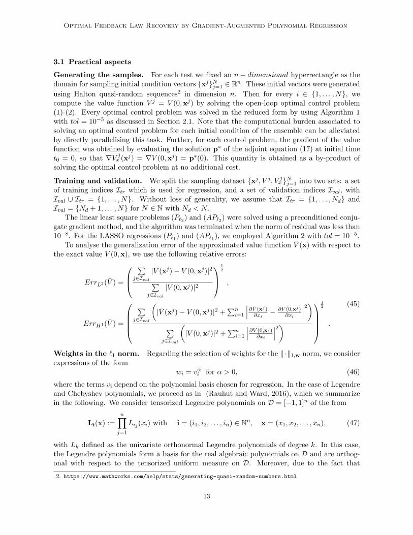
We computed the solutions θ`2 , θ`2 , θ`1 and θ`1 to the problems (P`2) , (AP`2), (P`1), and(AP`1), respectively, analysing different sizes for the training dataset Nd, the choice of `1 weightsencoded through α in (46), and polynomial bases. A compact summary of these results is givenin Table 1. The first column gives the errors of the value function and the nonzero componentsin its expansion without relying on gradient information and without sparsification. In thesecond column gradient information is added and the errors decrease for the same number oftraining samples (Nd = 40). For the third column the sparsity enhancing functional is addedand approximately the same errors are obtained with significantly fewer nonzero components inthe expansion.

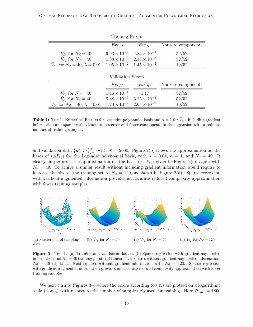
To illustrate the approximation of the value function V (x) by the different regression formu-lations, we consider Figure 2(a). This figure displays the scatter plot associated to the training

14


Training Errors

ErrL2 ErrH1 Nonzero components

V`2 for Nd = 40 9.93× 10−9 4.83× 10−1 52/52V`2 for Nd = 40 1.38× 10−3 2.34× 10−3 52/52

V`1 for Nd = 40, λ = 0.01 1.05× 10−2 1.45× 10−2 19/52

Validation Errors


V`2 for Nd = 40 1.46× 10−1 1.17 52/52V`2 for Nd = 40 9.38× 10−3 3.25× 10−2 52/52

V`1 for Nd = 40, λ = 0.01 1.20× 10−2 2.05× 10−2 19/52

Table 1: Test 1. Numerical Results for Legendre polynomial basis and α = 1 for V`1 . Including gradientinformation and sparsification leads to less error and fewer components in the expansion with a reducednumber of training samples.

and validation data xj , V jNj=1 with N = 2000. Figure 2(b) shows the approximation on thebases of (AP`1) for the Legendre polynomial basis, with λ = 0.01, α = 1, and Nd = 40. Itclearly outperforms the approximation on the basis of (P`2) given in Figure 2(c), again withNd = 40. To achive a similar result without including gradient information would require toincrease the size of the training set to Nd = 120, as shown in Figure 2(d). Sparse regressionwith gradient-augmented information provides an accurate reduced complexity approximationwith fewer training samples.

(a) Scatter plot of samplingdata

(b) V`1 for Nd = 40 (c) V`2 for Nd = 40 (d) V`2 for Nd = 120

Figure 2: Test 1. (a) Training and validation dataset (b) Sparse regression with gradient-augmentedinformation andNd = 40 training points (c) Linear least squares without gradient-augmented information,Nd = 40 (d) Linear least squares without gradient information with Nd = 120. Sparse regressionwith gradient-augmented information provides an accurate reduced complexity approximation with fewertraining samples.

We next turn to Figures 3–6 where the errors according to (45) are plotted on a logarithmicscale ( log10) with respect to the number of samples Nd used for training. Here |Ival| = 1800

15


validation samples were used. For problem (P`1) and (AP`1) we chose the sparse penalty param-eter λ = 0.002 and λ = 0.01, 0.02, respectively. Choosing λ larger for (AP`1) than for (P`1)allows to approximately balance the contributions for the data and the regularization terms inthe cost functionals of these two problems. The cardinality of the non-zero coefficients of θ`1 andθ`1 is determined by defining components as nonzero if its absolute value is bigger than doublemachine extended precision 10−20. Let us next make some observations on these results.

As expected, the error decreases with the training size Nd, up to a certain threshold. Thebest possible fit for the chosen order s = 16 (q = 52) of the polynomial approximation is reachedat about Nd = 50 and Nd = 75 for Legendre and Chebyshev polynomials, respectively, withoutthe use of gradient information, see Figures 3 and 4. These error levels are reached much earlierwhen we include gradient information, as shown in Figures 5 and 6. The influence of the `1weights, expressed in terms of α, is not very pronounced. Note that α = −∞ corresponds to noregularisation, whereas α = 0 corresponds to a constant weight. In the case that Nd ≪ 52, thesystem is highly under-determined for α = −∞, which goes along with a large error. For smallNd, the choice α = 2 can be favoured over the choice α = 0, with the latter giving best resultsfor Nd sufficiently large.

In the last column of these plots the cardinality of nonzero coefficients for θ`1 is depicted. Ittypically increases with Nd up to a certain threshold, and roughly stays constant thereafter, atless than 50 percent of the total number of free coefficients. Increasing λ promotes sparsity, asexpected, see Figures 5 -6, (c) and (f).

Nd

50 100 15010

-3

10-2

10-1

100

ErrH1(V )

α = −∞

α = 2α = 1α = 0.5α = 0

(a) λ = 0.002

Nd

50 100 15010

-3

10-2

10-1

100

ErrL2(V )

α = −∞

α = 2α = 1α = 0.5α = 0

(b) λ = 0.002

Nd

50 100 1500

10

20

30

40

50

Number of non-zero components

α = 1

α = 0

(c) λ = 0.002

Figure 3: Test 1. Numerical results for the polynomial approximation without gradient informationusing the Legendre polynomial basis. Both H1 and L2 validation errors decrease as the number of trainingsamples increases for different weights in the `1 norm penalty. The sparse regression reduces the numberof non-zero coefficients in the feedback law expansion.

Figures 3 and 5 correspond to the Legendre polynomial basis, while Figures 4 and 6 areobtained with Chebyshev polynomials. The results are quite similar in terms of the asymptotic(with respect to Nd) behavior of the errors. The number of non-zero components is higher for theChebyshev than for the Legrendre polynomial expansion. By comparing Figures 5 (resp. Figure6 ) with 3 (resp. Figure 4 ), we can see that for obtaining the same precision of approximation weneed to consider more samples. As expected, for the case of gradient-augmented approximationwe obtained better results for the H1-errors for small Nd.

16


Nd

50 100 15010

-3

10-2

10-1

100

ErrH1(V )

α = −∞

α = 2α = 1α = 0.5α = 0

(a) λ = 0.002

Nd

50 100 15010

-3

10-2

10-1

100

ErrL2(V )

α = −∞

α = 2α = 1α = 0.5α = 0

(b) λ = 0.002

Nd

50 100 1500

10

20

30

40

50


α = 1

α = 0

(c) λ = 0.002

Figure 4: Test 1. Numerical results for the polynomial approximation without gradient informationsusing the Chebyshev polynomial basis. Results are qualitatively similar to those in Figure 3 for a Legendrebasis.

Nd

10 20 30 40 50 6010

-3

10-2

10-1

100

ErrH1(V )

α = −∞

α = 2α = 1α = 0.5α = 0

(a) λ = 0.01

Nd

10 20 30 40 50 6010

-3

10-2

10-1

100

ErrL2(V )

α = −∞

α = 2α = 1α = 0.5α = 0

(b) λ = 0.01

Nd

10 20 30 40 50 600

10

20

30

40

50


α = 1

α = 0

(c) λ = 0.01

Nd

10 20 30 40 50 6010

-3

10-2

10-1

100

ErrH1(V )

α = −∞

α = 2α = 1α = 0.5α = 0

(d) λ = 0.02

Nd

10 20 30 40 50 6010

-3

10-2

10-1

100

ErrL2(V )

α = −∞

α = 2α = 1α = 0.5α = 0

(e) λ = 0.02

Nd

10 20 30 40 50 600

10

20

30

40

50


α = 1

α = 0

(f) λ = 0.02

Figure 5: Test 1. Numerical results for the gradient-augmented polynomial approximation using theLegendre polynomial basis. Similarly to Figures 3 and 4, H1 and L2 validation errors decrease as thenumber of training samples increases. However, lower errors are reached with fewer samples due to theinclusion of gradient information, and without affecting the sparsity of the feedback law expansion.

Moreover, we approximated the optimal control by using (38) and (39). To be more precise,we compute the following feedback law:

uθ(x) = − 1

2β

∑i∈I

θi∇xΦi(x). (52)

17


Nd

10 20 30 40 50 6010

-3

10-2

10-1

100

ErrH1(V )

α = −∞

α = 2α = 1α = 0.5α = 0

(a) λ = 0.01

Nd

10 20 30 40 50 6010

-3

10-2

10-1

100

ErrL2(V )

α = −∞

α = 2α = 1α = 0.5α = 0

(b) λ = 0.01

Nd

10 20 30 40 50 600

10

20

30

40

50


α = 1

α = 0

(c) λ = 0.01

Nd

10 20 30 40 50 6010

-3

10-2

10-1

100

ErrH1(V )

α = −∞

α = 2α = 1α = 0.5α = 0

(d) λ = 0.02

Nd

10 20 30 40 50 6010

-3

10-2

10-1

100

ErrL2(V )

α = −∞

α = 2α = 1α = 0.5α = 0

(e) λ = 0.02

Nd

10 20 30 40 50 600

10

20

30

40

50


α = 1

α = 0

(f) λ = 0.02

Figure 6: Test 1. Numerical results for the gradient-augmented polynomial approximation using theChebyshev polynomial basis. Results are qualitatively similar to those in Figure 5 for the Legendre basis.

where ∇xΦi stands for the gradient of the polynomial basis. We applied this feedback law for thechoices θ`2 , θ`2 , and θ`1 for two initial vectors (2, 1) and (2,−1). The evolution of the norm forthe states controlled by these feedback laws, compared to the optimal state, and the uncontrolledstate is illustrated in Figures 7(a) and 8(a). Figures 7(b) and 8(b) depict the evolution of theabsolute value of the controls. Clearly, the controls uθ`2

and uθ`1on the basis of V`2 and V`1

approximate well the challenging behaviour of the optimal control, and they outperform uθ`2obtained by V`2 .

Another advantage of using a sparse regression is the synthesis of a feedback law of reducedcomplexity. This is particularly relevant for the implementation of feedback laws in a real-timeenvironment, where the number of calculations in the control loop needs to be minimized. Ingeneral, a feedback law expressed in the form

uθ(x) = − 1

2βg>(x)

∑i∈I

θi∇xΦi(x) , with g(x) ∈ Rn×m ,∇Φi(x) ∈ Rn , (53)

requires O((mn2 +n)q) floating-point operations, where q is the number of non-zero componentsin the expansion. Thus, the operation count decreases linearly with the level of sparsity. Goingback to Table 1, this implies a reduction of 63% in the number of operations with respect to an`2-based controller.

18


t0 1 2 3

0

0.5

1

1.5

2

2.5

‖y(t)‖ℓ2

APℓ2

UnCo

APℓ1

Pℓ2

Op

(a) State

t0 1 2 3

0

0.5

1

1.5

2

|u(t)|

APℓ2

APℓ1

Pℓ2

Op

(b) Control

Figure 7: Test 1. Evolution of ‖y(t)‖`2 and |u(t)| for x = (2,−1). Here UnCo stands for the uncontrolledtrajectory, and Op refers to the exact optimal trajectory. We observe that the optimal feedback lawobtained from the gradient-augmented sparse polynomial regression follows the true optimal trajectory,unlike the feedback law computed without gradient information.

t0 1 2 3

0

0.5

1

1.5

2

2.5

‖y(t)‖ℓ2

APℓ2

UnCo

APℓ1

Pℓ2

Op

(a) State

t0 1 2 3

0

2

4

6

8

|u(t)|

APℓ2

APℓ1

Pℓ2

Op

(b) Control

Figure 8: Test 1. Evolution of ‖y(t)‖`2 and |u(t)| for x = (2, 1). Here UnCo stands for the uncontrolledtrajectory, and Op refers to the exact optimal trajectory. Results are qualitatively similar to Figure 7(b).

3.3 Test 2: Controlled Allen-Cahn equation

In the following test, we consider the PDE-constrained optimal control problem

minu∈L2(0,T ;R2)

∫ T

0(‖y(t)‖2L2(0,1) + β‖u(t)‖22)dt (54)

subject to ∂ty − ν∂2

xy − y(1− y2) =∑3

i=1 ui(t)1ωi in (0, T )× Ω,

∂xy(t, 1) = ∂xy(t, 0) = 0 in (0, T ),

y(0, y) = y0 in Ω,

(55)

with the 3-d control vector u(t) := [u1(t), u2(t), u3(t)] ∈ L2(0, 4;R3), Ω = (−1, 1), ν = 0.1,β = 0.01 and T = 4. The control signals act through 1ωi = 1ωi(x), which denote the indicatorfunctions with supports ω1 = (−0.7,−0.4), ω2 = (−0.2, 0.2), and ω3 = (0.4, 0.7). Due to theinfinite-dimensional nature of the state equation this problem does not fall directly into theoptimal control setting considered in this paper. We first perform an approximation of (55) inspace by doing a pseudospectral collocation using Chebyshev spectral elements with 18 degrees

19


of freedom as in (Kalise and Kunisch, 2018). This approximates the PDE control dynamics as an18-dimensional nonlinear dynamical system. The resulting ODE system was treated numericallyby the Crank-Nicolson time stepping method with step-size ∆t = 0.005. Subsequently, a datasetxj , V j , V j

x Nj=1 with N = 9000 (including samples for training and validation) was generated bysolving open-loop problem (54)-(55) for different values of quasi-randomly chosen initial vectorsfrom the hypercube [−10, 10]18.

For this example we used the two different values s = 4 and s = 8 in the hyperbolic crossindex set I(s). For these choices we have |I(4)| = 226 and |I(8)| = 1879, resulting in 226 (resp.1897) polynomial basis functions to approximate the value functions V := V (0, ·). We computedthe solutions θ`2 , θ`2 , θ`1 and θ`1 to problems (P`2) , (AP`2), (P`1), and (AP`1) for the differentchoices of Nd, α, and polynomial basis. For problems (P`1) and (AP`1) we show results withλ = 0.01 and λ = 0.008, 0.04, respectively, using Chebyshev polynomials. Similarly as in Test1, we report the level of non-sparsity of θ`1 , θ`1 . The errors (45) are shown for a validation setwith |Ival| = 5000 samples. These results are depicted in Figures 9 and 10.

Overall, these results allow to draw the same conclusions as for the previous test. In par-ticular, as Nd increases, the validation errors are getting smaller. Again, comparing Figures 9and 10 the gradient-augmented results reach the lowest errors with significantly smaller datasetsNd than the gradient-free ones. Figures 9-10 also confirm that the errors for s = 8 are smallercompared to s = 4. Naturally, for polynomials basis associated to s = 8, we need to increasethe training data in comparison to s = 4. Comparing rows 1 and 2 in Figure 9, we observe thatdecreasing λ results in an increase on the number of non-zero components and in a decrease ofthe errors.

We approximated the optimal control using (39) and (38), resulting in the feedback law

uθ(x) = − 1

2βg>∑i∈I

θi∇xΦi(x) , (56)

where g := [1ω1 |1ω2 |1ω3 ] ∈ Rn×3. We applied this feedback law for the choices θ`2 , θ`2 , and θ`1on the initial condition

y0(x) = (x− 1)(x+ 1) + 5. (57)

We report the results for the Chebyshev polynomial basis with s = 4 and thus q = 226. Forthe case θ`1 we set λ = 0.008 and α = 1. The evolution of the norm of the resulting controlled,optimal, and uncontrolled states are depicted in Figures 11(a), and the associated controls in11(b).

Figure 12(a) depicts the uncontrolled state. It converges to the stable equilibrium given bythe constant function with value 1. The state controlled by uθ`1 is illustrated in Figure 12(b).Here the state tends to 0 as expected.

3.4 Test 3: Optimal consensus control in the Cucker-Smale model

We conclude with a thorough discussion of a high-dimensional, non-linear, non-local optimalcontrol problem related to consensus control of agent-based dynamics (Bailo et al., 2018; Bonginiet al., 2015; Caponigro et al., 2015). We study the Cucker-Smale model (Cucker and Smale,2007) for consensus control with Na agents with states (yi, vi) ∈ Rd×Rd for i = 1, . . . , Na, whereyi and vi stand for the position and velocity of the i-th agent, respectively, and d ∈ N is the

20


Nd

10 20 30 40

10-1

100

ErrH1(V )

α = −∞

α = 2α = 1α = 0.5α = 0

(a) s = 4, λ = 0.04

Nd

10 20 30 40

10-1

100

ErrL2(V )

α = −∞

α = 2α = 1α = 0.5α = 0

(b) s = 4, λ = 0.04

Nd

0 10 20 30 400

50

100

150

200


α = 1

α = 0

(c) s = 4, λ = 0.04

Nd

10 20 30 40

10-1

100

ErrH1(V )

α = −∞

α = 2α = 1α = 0.5α = 0

(d) s = 4, λ = 0.008

Nd

10 20 30 40

10-1

100

ErrL2(V )

α = −∞

α = 2α = 1α = 0.5α = 0

(e) s = 4, λ = 0.008

Nd

0 10 20 30 400

50

100

150

200


α = 1

α = 0

(f) s = 4, λ = 0.008

Nd

100 200 300 400

10-1

100

ErrH1(V )

α = −∞

α = 2α = 1α = 0.5α = 0

(g) s = 8, λ = 0.008

Nd

100 200 300 400

10-1

100

ErrL2(V )

α = −∞

α = 2α = 1α = 0.5α = 0

(h) s = 8, λ = 0.008

Nd

0 100 200 300 4000

500

1000

1500


α = 1

α = 0

(i) s = 8, λ = 0.008

Figure 9: Test 2. Numerical results for the gradient-augmented polynomial approximation using theChebyshev polynomial basis. Due to the inclusion of gradient-augmented information in the training,the validation error in the H1 and L2 norms decrease as the number of samples is moderately increased.The sparsity pattern of the resulting feedback law can be controlled through the parameter α whichdetermines the weight in the `1-norm penalty term.

dimension of the physical space. Then dynamics of the agents are governed by

dyidt

= vi ,

dvidt

=1

Na

Na∑j=1

vj − vi1 + ‖yi − yj‖2

+ ui , i = 1, . . . , Na ,

yi(0) = xi , vi(0) = wi .

(58)

21


Nd

100 200 300 400

10-1

100

ErrH1(V )

α = −∞

α = 2α = 1α = 0.5α = 0

(a) s = 4, λ = 0.01

Nd

100 200 300 400

10-1

100

ErrL2(V )

α = −∞

α = 2α = 1α = 0.5α = 0

(b) s = 4, λ = 0.01

Nd

100 200 300 4000

50

100

150

200


α = 1

α = 0

(c) s = 4, λ = 0.01

Nd

1000 2000 3000 4000

10-1

100

ErrH1(V )

α = −∞

α = 2α = 1α = 0.5α = 0

(d) s = 8, λ = 0.01

Nd

1000 2000 3000 4000

10-1

100

ErrL2(V )

α = −∞

α = 2α = 1α = 0.5α = 0

(e) s = 8, λ = 0.01

Nd

1000 2000 3000 40000

500

1000

1500


α = 1

α = 0

(f) s = 8, λ = 0.01

Figure 10: Test 2. Numerical results for the polynomial approximation without gradient informationsusing the Chebyshev polynomial basis. Results are qualitatively similar to Figure 9 with the Legendrepolynomial basis.

t0 1 2 3 4

0

5

10

15

‖y(t)‖L2(Ω)

APℓ2 with Nd = 34UnCo

APℓ1 with Nd = 34Pℓ2 with Nd = 646Pℓ2 with Nd = 510Op

t0 1 2 3 4

-5

-4

-3

-2

-1

0

1

2

3

log10(‖u(t)‖ℓ2)

APℓ2 with Nd = 34APℓ1 with Nd = 34Pℓ2 with Nd = 646Pℓ2 with Nd = 510Op

Figure 11: Test 2. Evolution of ‖y(t)‖L2(Ω) and log10(‖u(t)‖) for the choices λ = 0.008, α = 1, andChebyshev polynomial basis.The gradient-augmented feedback laws outperform, both in stabilization andcontrol energy, the control laws recovered without gradient information.

The consensus control problem consists of finding a control u(t) := (u1(t), . . . , uNa(t)) ∈ Rd×Nawhich steers the system towards the consensus manifold

vi = v =1

Na

Na∑j=1

vj , ∀i = 1, . . . , Na . (59)

22


(a) Uncontrolled (b) Controlled

Figure 12: Test 2. The uncontrolled state and the controlled state by uθ`1 for Nd = 34, λ = 0.008,α = 1, and α = 1. The recovered feedback law effectively stabilizes the state of the system around theequilibrium y ≡ 0.

Asymptotic consensus emergence is conditional to the cohesiveness of the initial state x0 =(x1, . . . , xNa) and w0 = (w1, . . . , wNa) (Cucker and Smale, 2007). To remove this dependenceon the initial state, we cast this problem as an optimal control problem by defining the followingcost functional

J(u;x0,w0) :=

∫ >0

Na∑i=1

1

Na‖vi(t)− v‖2 + β‖ui(t)‖2 dt, (60)

and formulating the optimal control problem

minu∈L2(0,T ;Rd×Na )

J(u;x0,v0) subject to (58). (OC(x0))

For the sake of completeness, in this case the adjoint system is given by (Bailo et al., 2018)

−dpyidt

=1

Na

∑j 6=i

−2(pvj − pvi)(1 + ‖yj − yi‖2)2

[(yi − yj)⊗ (vi − vj)] , (61)

−dpvidt

= pyi +1

Na

∑j 6=i

pvj − pvi1 + ‖yi − yj‖2

+2

N(vi − v)> i = 1, . . . , Na , (62)

pyi(T ) = 0, pvi(T ) = 0 , (63)

and the optimality condition reads

pvi(t) + 2βu∗i (t) = 0 ∀ t ∈ (0, T ) , i = 1, . . . , N . (64)

We denote the augmented initial state x0 = (x0,w0), and we approximate the value func-tion V (x) = V (0, x). We set Na = 20, d = 2, T = 10, and β = 0.01, and we compute adataset xj , V j , V j

x Nj=1 with N = 104. For every j, the initial vectors xj ∈ R80 were chosen

quasi-randomly from the hypercube [−3, 3]80. The dataset was computed by solving open-loop

23


problems with a time discretization using the fourth order Runge-Kutta method with step-size∆t = 0.01.

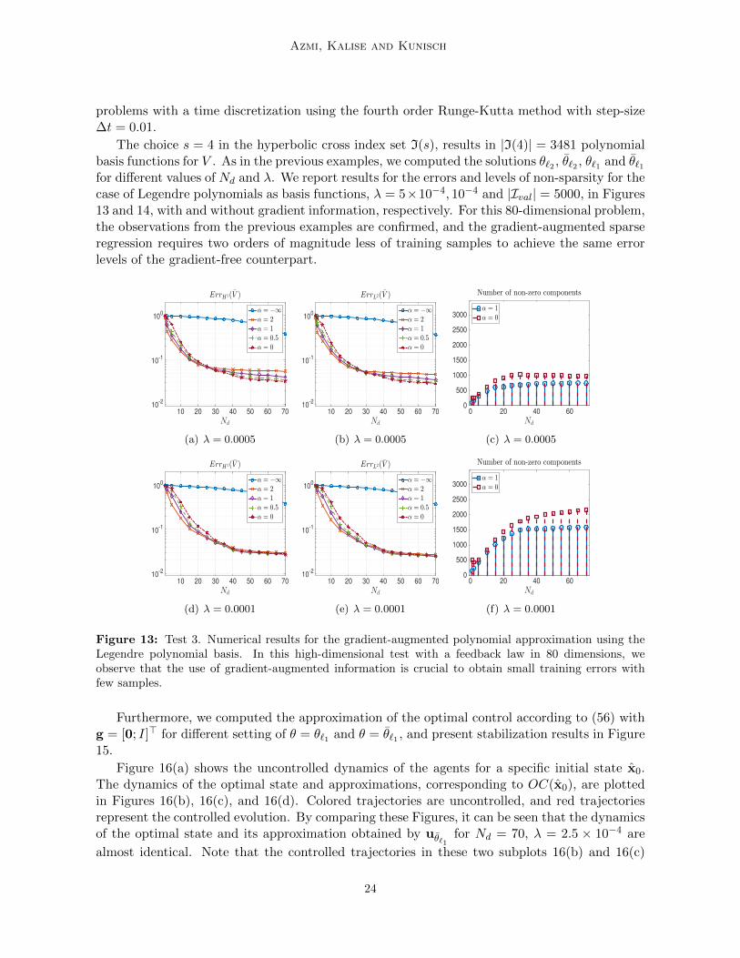
The choice s = 4 in the hyperbolic cross index set I(s), results in |I(4)| = 3481 polynomialbasis functions for V . As in the previous examples, we computed the solutions θ`2 , θ`2 , θ`1 and θ`1for different values of Nd and λ. We report results for the errors and levels of non-sparsity for thecase of Legendre polynomials as basis functions, λ = 5×10−4, 10−4 and |Ival| = 5000, in Figures13 and 14, with and without gradient information, respectively. For this 80-dimensional problem,the observations from the previous examples are confirmed, and the gradient-augmented sparseregression requires two orders of magnitude less of training samples to achieve the same errorlevels of the gradient-free counterpart.

Nd

10 20 30 40 50 60 7010

-2

10-1

100

ErrH1(V )

α = −∞

α = 2α = 1α = 0.5α = 0

(a) λ = 0.0005

Nd

10 20 30 40 50 60 7010

-2

10-1

100

ErrL2(V )

α = −∞

α = 2α = 1α = 0.5α = 0

(b) λ = 0.0005

Nd

0 20 40 600

500

1000

1500

2000

2500

3000


α = 1

α = 0

(c) λ = 0.0005

Nd

10 20 30 40 50 60 7010

-2

10-1

100

ErrH1(V )

α = −∞

α = 2α = 1α = 0.5α = 0

(d) λ = 0.0001

Nd

10 20 30 40 50 60 7010

-2

10-1

100

ErrL2(V )

α = −∞

α = 2α = 1α = 0.5α = 0

(e) λ = 0.0001

Nd

0 20 40 600

500

1000

1500

2000

2500

3000


α = 1

α = 0

(f) λ = 0.0001

Figure 13: Test 3. Numerical results for the gradient-augmented polynomial approximation using theLegendre polynomial basis. In this high-dimensional test with a feedback law in 80 dimensions, weobserve that the use of gradient-augmented information is crucial to obtain small training errors withfew samples.

Furthermore, we computed the approximation of the optimal control according to (56) withg = [0; I]> for different setting of θ = θ`1 and θ = θ`1 , and present stabilization results in Figure15.

Figure 16(a) shows the uncontrolled dynamics of the agents for a specific initial state x0.The dynamics of the optimal state and approximations, corresponding to OC(x0), are plottedin Figures 16(b), 16(c), and 16(d). Colored trajectories are uncontrolled, and red trajectoriesrepresent the controlled evolution. By comparing these Figures, it can be seen that the dynamicsof the optimal state and its approximation obtained by uθ`1

for Nd = 70, λ = 2.5 × 10−4 are

almost identical. Note that the controlled trajectories in these two subplots 16(b) and 16(c)

24


Nd

1000 2000 3000 400010

-2

10-1

100

ErrH1(V )

α = −∞

α = 2α = 1α = 0.5α = 0

(a) λ = 0.0005

Nd

1000 2000 3000 400010

-2

10-1

100

ErrL2(V )

α = −∞

α = 2α = 1α = 0.5α = 0

(b) λ = 0.0005

Nd

1000 2000 3000 40000

500

1000

1500

2000

2500

3000


α = 1

α = 0

(c) λ = 0.0005

Figure 14: Test 3. Numerical results of the polynomial approximation using the Legendre basis withoutgradient information. Compared to Figure 13, the number of samples required to reach similar errors isalmost 2 orders of magnitude larger, as this regression does not include gradient measurements.

t0 2 4 6 8 10

0

0.1

0.2

0.3

0.4

0.5

1N

∑Ni=1 ‖vi(t)− v‖2

APℓ1 with Nd = 30, λ = 0.005APℓ1 with Nd = 50, λ = 0.00075APℓ1 with Nd = 70, λ = 0.00025Pℓ1 with Nd = 2430, λ = 0.00025Pℓ1 with Nd = 4455, λ = 0.0001Op

UnCo

(a) State

t0 2 4 6 8 10

0

1

2

3

4

5

6

7

‖u(t)‖

APℓ1 with Nd = 30, λ = 0.005APℓ1 with Nd = 50, λ = 0.00075APℓ1 with Nd = 70, λ = 0.00025Pℓ1 with Nd = 2430, λ = 0.00025Pℓ1 with Nd = 4455, λ = 0.0001Op

(b) Control

Figure 15: Test 3. (a) Evolution of the consensus variance 1Na

∑Na

i=1 ‖vi(t)−v‖2 for different control lawsand (b) the norm ‖u(t)‖ of the associated control signals. Here Op stands for the exact optimal control,and UnCo for the uncontrolled solution. Recovered feedback laws including gradient information and asmall number of samples (50 and 70 in this case) effectively stabilize the dynamics around consensus,while a similar control law without gradient information requires over 4000 training samples.

achieve consensus, unlike 16(d), where the feedback obtained with a sparse regression withoutgradient information does not stabilize the dynamics despite the large training dataset. Thisobservation is also supported by Table 2 and Figure (15). Table 2 shows that the smallestvalidation error is achieved for the gradient-augmented sparse regression of the value functionwith only 70 training samples, with approximately 20% of nonzero components. Figure (15)depicts the evolution of the tracking term 1

Na

∑Nai=1 ‖vi(t) − v‖2 and the norm of the control of

every feedback law. From this figure, we can see that the control uθ`1associated to Nd = 70,

λ = 2.5 × 10−4 delivers the best approximation for the optimal control of OC(x0) among thedifferent control laws.

25


-10 -5 0 5-10

-5

0

5

10

15

(a) Uncontrolled State

-2 -1 0 1 2-1.5

-1

-0.5

0

0.5

1

1.5

2

2.5

3

(b) Optimal state

-2 -1 0 1 2 3-1.5

-1

-0.5

0

0.5

1

1.5

2

2.5

3

3.5

(c) AP`1 withNd = 70, λ =2.5 × 10−4

-2 -1 0 1 2 3 4-2

-1

0

1

2

3

4

5

6

(d) P`1 with Nd = 2430,λ = 2.5 × 10−4

Figure 16: Test 3. Trajectories generated by different control laws. (a) Uncontrolled trajectoriesdiverging in space. (b) Optimal trajectory for reference. In this high-dimensional problem (n = 80), thesparse, gradient-augmented regression for V (c) yields an feedback law which approaches the optimaltrajectory (b) with few training samples Nd = 70. In (d) we observe a controlled trajectory with afeedback law without gradient information and an insufficient number of samples, which fails to stabilizethe dynamics.


V`1 for Nd = 50, λ = 7.5× 10−4 5.40× 10−2 6.37× 10−2 393/3481V`1 for Nd = 70, λ = 2.5× 10−4 3.56× 10−2 4.11× 10−2 738/3481V`1 for Nd = 2430, λ = 2.5× 10−4 7.46× 10−2 9.38× 10−2 656/3481

Table 2: Test 3. Validation errors for different regressions. The use of gradient-augmented informationfor the regression leads to the recovery of high-dimensional feedback laws with a reduced number oftraining samples. The inclusion of a sparsity promoting term in the regression reduces to the number ofnon-zero components in the control law to less than 15%.

Concluding remarks

We have presented a sparse polynomial regression framework for the approximation of feedbacklaws arising in nonlinear optimal control. The main ingredients of our approach include: thegeneration of a gradient-augmented dataset for the value function associated to the controlproblem by means of PMP solves, a hyperbolic cross polynomial ansatz for recovering the valuefunction and its feedback law, and a sparse optimization method to fit the model. Througha series of numerical tests, we have shown that the proposed approach can approximate high-dimensional control problems at moderate computational cost. It is worth to note that ournumerical tests correspond to smooth value functions, where gradients are regular and theirinclusion in the regression is well-posed. The gradient-augmented dataset reduces the numberof open-loop solves required to recover the optimal control, and the sparse regression provides afeedback law of reduced complexity, which is an appealing feature for real-time implementations.The effectiveness of the proposed methodology suggests different research directions:

• The deep neural network ansatz proposed in (Nakamura-Zimmerer et al., 2019) can becombined with a sparsity-promoting loss function along the lines of our work. In the lightof recent results discussed in (Adcock and Dexter, 2020), it is a pertinent question to findwhether deep neural networks or polynomial approximants are more effective ansatz for the

26


value function. As we have previously mentioned, there are different control-theoreticalarguments which support the case for having a polynomial approximation of the valuefunction.

• The study of the regression framework in control problems with a fully nonlinear controlstructure. For the sake of simplicity, we have restricted our problem formulation to thecontrol-affine case, however, the link between PMP and HJB holds in the fully nonlinearcase under standard regularity assumptions (Subbotina, 2004, Section 3.2). Nevertheless,the nonlinear control structure can deteriorate the approximation power of the hyperboliccross ansatz for the value function. Moreover, dataset generation in the fully nonlinearcase can be costly as the structure of (TPBVP) becomes more complex.

• The extension of the presented results in the context to time-dependent, and second-orderstochastic control problems where the representation formula given by the PMP is replacedby a backward stochastic differential equation (Gnoatto et al., 2020). Finally, the ideasproposed in this work regarding sparse polynomial regression can be implemented in thecontext of approximate dynamic programming in reinforcement learning (Bertsekas, 2019).

Acknowledgments

Dante Kalise was supported by a public grant as part of the Investissement d’avenir project,reference ANR-11-LABX-0056-LMH, LabEx LMH. Karl Kunisch was supported in part by theERC advanced grant 668998 (OCLOC) under the EU’s H2020 research program.

References

Taylor expansions of the value function associated with a bilinear optimal control problem. Ann.Inst. H. Poincare Anal. Non Lineaire, 36(5):1361 – 1399, 2019.

Computing Lyapunov functions using deep neural networks, 2020.

B. Adcock and N. Dexter. The gap between theory and practice in function approximation withdeep neural networks, 2020. arXiv preprint: 2001.07523.

B. Adcock and Y. Sui. Compressive Hermite interpolation: sparse, high-dimensional approxi-mation from gradient-augmented measurements. Constr. Approx., 50(1):167–207, 2019.

B. Adcock, S. Brugiapaglia, and C. G. Webster. Compressed sensing approaches for polynomialapproximation of high-dimensional functions. In Compressed sensing and its applications,Appl. Numer. Harmon. Anal., pages 93–124. Birkhauser/Springer, Cham, 2017.

B. Adcock, A. Bao, and S. Brugiapaglia. Correcting for unknown errors in sparse high-dimensional function approximation. Numer. Math., 142(3):667–711, 2019.

M. Akian, S. Gaubert, and A. Lakhoua. The max-plus finite element method for solving de-terministic optimal control problems: basic properties and convergence analysis. SIAM J.Control Optim., 47(2):817–848, 2008.

27


G. Albi, Y.-P. Choi, M. Fornasier, and D. Kalise. Mean field control hierarchy. Appl. Math.Optim., 76(1):93–135, 2017.

E. Al’brekht. On the optimal stabilization of nonlinear systems. Journal of Applied Mathematicsand Mechanics, 25(5):1254, 1961.

A. Alla, M. Falcone, and L. Saluzzi. An efficient DP algorithm on a tree-structure for finitehorizon optimal control problems. SIAM J. Sci. Comput., 41(4):A2384–A2406, 2019.

B. Azmi and K. Kunisch. On the stabilizability of the Burgers equation by receding horizoncontrol. SIAM J. Control Optim., 54(3):1378–1405, 2016.

B. Azmi and K. Kunisch. Analysis of the Barzilai-Borwein step-sizes for problems in Hilbertspaces. J. Optim Theory Appl., 185:819–844, 2020.

R. Bailo, M. Bongini, J. A. Carrillo, and D. Kalise. Optimal consensus control of the cucker-smale model. IFAC-PapersOnLine, 51(13):1 – 6, 2018.

M. Bardi and I. Capuzzo-Dolcetta. Optimal control and viscosity solutions of Hamilton-Jacobi-Bellman equations. Systems & Control: Foundations & Applications. Birkhauser Boston, Inc.,Boston, MA, 1997. With appendices by Maurizio Falcone and Pierpaolo Soravia.

E. N. Barron and R. Jensen. The Pontryagin maximum principle from dynamic programmingand viscosity solutions to first-order partial differential equations. Trans. Amer. Math. Soc.,298(2):635–641, 1986.

J. Barzilai and J. M. Borwein. Two-point step size gradient methods. IMA J. Numer. Anal., 8(1):141–148, 1988.

A. Beck. First-order methods in optimization, volume 25 of MOS-SIAM Series on Optimization.Society for Industrial and Applied Mathematics (SIAM), Philadelphia, PA; MathematicalOptimization Society, Philadelphia, PA, 2017.

J. Beck, R. Tempone, F. Nobile, and L. Tamellini. On the optimal polynomial approximationof stochastic PDEs by Galerkin and collocation methods. Math. Models Methods Appl. Sci.,22(9):1250023, 33, 2012.

S. C. Beeler, H. T. Tran, and H. T. Banks. Feedback control methodologies for nonlinear systems.J. Optim. Theory Appl., 107(1):1–33, 2000.

R. Bellman. Adaptive control processes: A guided tour. Princeton University Press, Princeton,N.J., 1961.

D. P. Bertsekas. Reinforcement Learning and Optimal Control. Athena Scientific, Belmont, MA,2019.

O. Bokanowski, J. Garcke, M. Griebel, and I. Klompmaker. An adaptive sparse grid semi-Lagrangian scheme for first order Hamilton-Jacobi Bellman equations. J. Sci. Comput., 55(3):575–605, 2013.

M. Bongini, M. Fornasier, and D. Kalise. (Un)conditional consensus emergence under perturbedand decentralized feedback controls. Discrete Contin. Dyn. Syst., 35(9):4071–4094, 2015.

28


S. Boyd, N. Parikh, E. Chu, B. Peleato, J. Eckstein, et al. Distributed optimization and statisticallearning via the alternating direction method of multipliers. Foundations and Trends R© inMachine learning, 3(1):1–122, 2011.

T. Breiten, K. Kunisch, and S. S. Rodrigues. Feedback stabilization to nonstationary solutionsof a class of reaction diffusion equations of fitzhugh–nagumo type. SIAM J. Control Optim.,55(4):2684–2713, 2017.

P. Cannarsa and H. Frankowska. Some characterizations of optimal trajectories in control theory.SIAM J. Control Optim., 29(6):1322–1347, 1991.

P. Cannarsa and H. Frankowska. Local regularity of the value function in optimal control.Systems Control Lett., 62(9):791–794, 2013.

M. Caponigro, M. Fornasier, B. Piccoli, and E. Trelat. Sparse stabilization and control ofalignment models. Math. Models Methods Appl. Sci., 25(3):521–564, 2015.

A. Chkifa, A. Cohen, G. Migliorati, F. Nobile, and R. Tempone. Discrete least squares poly-nomial approximation with random evaluations - application to parametric and stochasticelliptic pdes. ESAIM: M2AN, 49(3):815–837, 2015a.

A. Chkifa, A. Cohen, and C. Schwab. Breaking the curse of dimensionality in sparse polynomialapproximation of parametric PDEs. J. Math. Pures Appl. (9), 103(2):400–428, 2015b.

Y.-P. Choi, D. Kalise, J. Peszek, and A. A. Peters. A collisionless singular Cucker-Smale modelwith decentralized formation control. SIAM J. Appl. Dyn. Syst., 18(4):1954–1981, 2019.

Y. T. Chow, J. Darbon, S. Osher, and W. Yin. Algorithm for overcoming the curse of dimension-ality for time-dependent non-convex Hamilton-Jacobi equations arising from optimal controland differential games problems. J. Sci. Comput., 73(2-3):617–643, 2017.

Y. T. Chow, J. Darbon, S. Osher, and W. Yin. Algorithm for overcoming the curse of di-mensionality for certain non-convex Hamilton-Jacobi equations, projections and differentialgames. Ann. Math. Sci. Appl., 3(2):369–403, 2018.

Y. T. Chow, J. Darbon, S. Osher, and W. Yin. Algorithm for overcoming the curse of di-mensionality for state-dependent Hamilton-Jacobi equations. J. Comput. Phys., 387:376–409,2019.

F. H. Clarke and R. B. Vinter. The relationship between the maximum principle and dynamicprogramming. SIAM J. Control Optim., 25(5):1291–1311, 1987.

A. Cohen, R. Devore, and C. Schwab. Analytic regularity and polynomial approximation ofparametric and stochastic elliptic PDE’s. Anal. Appl. (Singap.), 9(1):11–47, 2011.

E. Cristiani and P. Martinon. Initialization of the shooting method via the Hamilton-Jacobi-Bellman approach. J. Optim. Theory Appl., 146(2):321–346, Aug 2010.

F. Cucker and S. Smale. Emergent behavior in flocks. IEEE Trans. Automat. Control, 52(5):852–862, 2007.

29


Y.-H. Dai and H. Zhang. Adaptive two-point stepsize gradient algorithm. Numer. Algorithms,27(4):377–385, 2001.

J. Darbon and S. Osher. Algorithms for overcoming the curse of dimensionality for certainHamilton-Jacobi equations arising in control theory and elsewhere. Res. Math. Sci., 3:PaperNo. 19, 26, 2016.

J. Darbon, G. P. Langlois, and T. Meng. Overcoming the curse of dimensionality for someHamilton-Jacobi partial differential equations via neural network architectures, 2020.

S. Dolgov, D. Kalise, and K. Kunisch. Tensor Decompositions for High-dimensional Hamilton-Jacobi-Bellman Equations, 2019. arXiv preprint: 1908.01533.

M. Fornasier and F. Solombrino. Mean-field optimal control. ESAIM: COCV, 20(4):1123–1152,2014.

H. Frankowska. Value function in optimal control. In Mathematical control theory, Part 1, 2(Trieste, 2001), ICTP Lect. Notes, VIII, pages 516–653. Abdus Salam Int. Cent. Theoret.Phys., Trieste, 2002.

J. Garcke and A. Kroner. Suboptimal feedback control of PDEs by solving HJB equations onadaptive sparse grids. J. Sci. Comput., 70(1):1–28, 2017.

A. Gnoatto, A. Picarelli, and C. Reisinger. Deep xVA solver – A neural network based coun-terparty credit risk management framework, 2020. arXiv preprint: 2005.02633.

S. N. Gomes and G. A. Pavliotis. Mean field limits for interacting diffusions in a two-scalepotential. J. Nonlinear Sci., 28(3):905–941, 2018.

A. Gorodetsky, S. Karaman, and Y. Marzouk. High-dimensional stochastic optimal control usingcontinuous tensor decompositions. Int. J. Robot. Res., 37(2-3):340–377, 2018.

L. Grune and A. Rantzer. On the infinite horizon performance of receding horizon controllers.IEEE Trans. Automat. Control, 53(9):2100–2111, 2008.

J. Han, A. Jentzen, and W. E. Solving high-dimensional partial differential equations using deeplearning. Proc. Natl. Acad. Sci. USA, 115(34):8505–8510, 2018.

R. Herzog and K. Kunisch. Algorithms for PDE-constrained optimization. GAMM-Mitt., 33(2):163–176, 2010.

M. B. Horowitz, A. Damle, and J. W. Burdick. Linear Hamilton Jacobi Bellman equations inhigh dimensions. In 53rd IEEE Conference on Decision and Control, pages 5880–5887, 2014.

K. Ito and J. Schroeter. Reduced order feedback synthesis for viscous incompressible flows.Math. Comput. Modellingg, 33(1):173 – 192, 2001.

K. Ito, C. Reisinger, and Y. Zhang. A neural network-based policy iteration algorithm withglobal h2-superlinear convergence for stochastic games on domains. Found. Comput. Math.,2020. doi: 10.1007/s10208-020-09460-1.

30


D. Kalise and K. Kunisch. Polynomial approximation of high-dimensional Hamilton-Jacobi-Bellman equations and applications to feedback control of semilinear parabolic PDEs. SIAMJ. Sci. Comput., 40(2):A629–A652, 2018.

D. Kalise, S. Kundu, and K. Kunisch. Robust feedback control of nonlinear PDEs by numericalapproximation of high-dimensional Hamilton-Jacobi-Isaacs equations. SIAM J. Appl. Dyn.Syst., 19(2):1496–1524, 2020.

W. Kang and L. Wilcox. A Causality Free Computational Method for HJB Equations withApplication to Rigid Body Satellites. 2015. doi: 10.2514/6.2015-2009. AIAA Guidance,Navigation, and Control Conference.

W. Kang and L. C. Wilcox. Mitigating the curse of dimensionality: sparse grid characteristicsmethod for optimal feedback control and HJB equations. Comput. Optim. Appl., 68(2):289–315, 2017.

W. Kang, Q. Gong, and T. Nakamura-Zimmerer. Algorithms of Data Development For DeepLearning and Feedback Design, 2019. arXiv preprint:1912.00492.

A. Krener, C. Aguilar, and T. Hunt. Series solutions of HJB equations. In K. Huper andJ. Trumpf, editors, Mathematical System Theory – Festschrift in Honor of Uwe Helmke onthe Occasion of his Sixtieth Birthday, pages 247–260. CreateSpace, 2013.

K. Kunisch and D. Walter. Semiglobal optimal feedback stabilization of autonomous systemsvia deep neural network approximation, 2020. arXiv preprint:2002.08625.

L. Laurent, R. Le Riche, B. Soulier, and P.-A. Boucard. An overview of gradient-enhancedmetamodels with applications. Archives of Computational Methods in Engineering, 26(1):61–106, Jan 2019.

D. Lukes. Optimal regulation of nonlinear dynamical systems. SIAM Journal on Control, 7(1):75–100, 1969.

W. M. McEneaney. A curse-of-dimensionality-free numerical method for solution of certain HJBPDEs. SIAM J. Control Optim., 46(4):1239–1276, 2007.

T. Nakamura-Zimmerer, Q. Gong, and W. Kang. Adaptive Deep Learning for High-DimensionalHamilton-Jacobi-Bellman Equations, 2019. arXiv preprint:1907.05317.

N. Nusken and L. Richter. Solving high-dimensional Hamilton-Jacobi-Bellman pdes using neuralnetworks: perspectives from the theory of controlled diffusions and measures on path space,2020. arXiv preprint:2005.05409.

M. Oster, L. Sallandt, and R. Schneider. Approximating the stationary Hamilton-Jacobi-Bellman equation by hierarchical tensor products, 2019. arXiv preprint:1911.00279.

H. J. Pesch and M. Plail. The maximum principle of optimal control: a history of ingeniousideas and missed opportunities. Control Cybernet., 38(4A):973–995, 2009.

L. S. Pontryagin, V. G. Boltyanskii, R. V. Gamkrelidze, and E. F. Mishchenko. The mathematicaltheory of optimal processes. Translated from the Russian by K. N. Trirogoff; edited by L. W.Neustadt. Interscience Publishers John Wiley & Sons, Inc. New York-London, 1962.

31


H. Rauhut and R. Ward. Interpolation via weighted `1 minimization. Appl. Comput. Harmon.Anal., 40(2):321–351, 2016.

M. Reble and F. Allgower. Unconstrained model predictive control and suboptimality estimatesfor nonlinear continuous-time systems. Automatica J. IFAC, 48(8):1812–1817, 2012.

E. Sarmin and L. Chudov. On the stability of the numerical integration of systems of ordinarydifferential equations arising in the use of the straight line method. USSR ComputationalMathematics and Mathematical Physics, 3(6):1537 – 1543, 1963.

E. Stefansson and Y. P. Leong. Sequential alternating least squares for solving high dimensionallinear Hamilton-Jacobi-Bellman equation. In 2016 IEEE/RSJ International Conference onIntelligent Robots and Systems (IROS), pages 3757–3764, 2016.

N. N. Subbotina. The method of characteristics for the Hamilton-Jacobi equations and itsapplications in dynamic optimization. Sovrem. Mat. Prilozh., (20, Differ. Uravn.):3–132,2004. ISSN 1512-1712. English translation appeared in Journal of Mathematical Sciences(New York) [135 (2006), no. 3].

K. Worthmann, M. Reble, L. Grune, and F. Allgower. The role of sampling for stability andperformance in unconstrained nonlinear model predictive control. SIAM J. Control Optim.,52(1):581–605, 2014.

I. Yegorov and P. M. Dower. Perspectives on Characteristics Based Curse-of-Dimensionality-Free Numerical Approaches for Solving Hamilton–Jacobi Equations. Appl. Math. Optim., Jul2018. doi: 10.1007/s00245-018-9509-6.

I. Yegorov, P. M. Dower, and L. Grune. Synthesis of control lyapunov functions and stabilizingfeedback strategies using exit-time optimal control, 2019. arXiv preprint:1906.02703.

32

Optimal Feedback Law Recovery by Gradient-Augmented Sparse ...

Documents

Transcript of Optimal Feedback Law Recovery by Gradient-Augmented Sparse ...