Optical Holography Reconstruction of...

9

Optical Holography Reconstruction of Nano-objects

Cesar A. Sciammarella1,2, Luciano Lamberti2 and

Federico M. Sciammarella1 1College of Engineering & Engineering Technology, Northern Illinois University,

2Dipartimento di Ingegneria Meccanica e Gestionale, Politecnico di Bari, 1USA 2Italy

1. Introduction

The continuous growth of many fields in nanoscience and nanotecnology puts the demand

for observations at the sub-micron level. Electron microscopy and X-rays can provide the

necessary short wavelengths to gather information at the nanometer and sub-nanometer

range but, in their current form, are not well suited to perform observations in many

problems of scientific and technical interest. Furthermore, the environment required for the

observation via X-rays or electron microscopy is not suitable for some type of specimens

that it is necessary to study. Another concern is the changes that may be induced in the

specimen’s structure by the utilized radiation. These issues have led to the return to optics

and to the analysis of the optical problem of “super-resolution” , that is the capacity of

producing optical images beyond the classical diffraction limit.

Classical optics has limitations on the resolution that can be achieved utilizing optical

microscopy in the observation of events taking place at the sub-micron level, i.e. to a few

hundreds of nanometers. To overcome this limitation and achieve super-resolution, non

conventional methods of illumination such as evanescent waves are utilized. The initial

approach to the utilization of evanescent field properties was the creation of near-field

techniques: a probe with dimensions in the nano-range detects the local evanescent field

generated in the vicinity of the objects that are observed. A perspective review on super-

resolution can be found in Sciammarella (2008).

New methods recently developed by C.A. Sciammarella and his collaborators (see, for

example, Sciammarella, 2008; Sciammarella et al., 2009) rely on the emission of coherent light

by the objects that are under analysis. This is done through the phenomenon of light

generation produced by electromagnetic resonance. Object self-luminosity is the consequence

of electromagnetic resonance. Why self-luminosity may help to increase resolution? The

light generated in this way has particular properties that are not present in the light sent by

an object that results from external illumination. The produced wave fronts can travel long

distances or go through an optical system without the diffraction changes experienced by

ordinary wave fronts (see, for example, Durnin et al., 1987; Buchal, 2003; Gutierrez-Vega et

al., 2001; Hernandez-Aranda et al., 2006).

www.intechopen.com

Holography, Research and Technologies

192

This paper will discuss two alternative approaches to near field techniques: (i) Using

diffraction through the equivalent of a diffraction grating to generate an ample spectrum of

wave vectors; (ii) Exciting the objects to be observed with the evanescent fields so that the

objects become self-luminous. Examples of optical holography reconstruction of nano-

objects are presented in the chapter.

The paper is structured as follows. After the Introduction section, evanescent waves and

super-resolution are briefly recalled in Section 2. Section 3 describes the experimental setup.

Section 4 analyzes the diffraction pattern of a 6 μm diameter polystyrene microsphere

immersed in a NaCl solution and illuminated by evanescent light. Section 5 analyzes the

system of rectilinear fringes observed in the image. Section 6 describes the process of

formation of holograms at the nano-scale. Sections 7 and 8 respectively present the results of

optical reconstruction of NaCl nanocrystals and polystyrene nanospheres contained in the

saline solution. Finally, Section 9 summarizes the most important findings of this study.

2. Theoretical background

2.1 Properties of evanescent waves The self generation of light is achieved through the use of total internal reflection (TIR). At

the interface between two media such that the index of refraction of medium 1 is larger than

the index of refraction of medium 2 (i.e. n1>n2), if a light beam is incident with an angle

θi>θi,crit, a total reflection of the beam, in which essentially all of the light is reflected back

into the first medium, takes place (Fig. 1a). Even though the light no longer propagates into

the second medium, there is a small amount of penetration of the electromagnetic field

across the interface between the two media. In the vector form solution of Maxwell

equations, it can be shown that, under the condition of total reflection, the electromagnetic

field does not disappear in the second medium (Born and Wolf, 1999). However, there is no

energy exchange with the second medium. The components of the electromagnetic field

transmitted in the second medium, vectors E and H, depend on (Born and Wolf, 1999):

2

212

sin2exp 1ii z

n

θπλ

⎡ ⎤⎢ ⎥− −⎢ ⎥⎣ ⎦ (1)

where the relative index of refraction is defined as n12=n2/ n1.

The intensity of the field decays by 1/ e at the distance z from the interface equal to:

2

212

sin2 1i

z

n

λθπ

=−

(2)

Under this condition a particular type of waves are produced in the interface (Fig. 1a). These

waves are called evanescent waves and travel at the interface decaying exponentially in the

second medium at a depth that is a fraction of the wavelength of the utilized light as shown

by Eq. (2). The decay of electromagnetic field is sketched in Fig. 1a.

The electromagnetic field of evanescent waves hence does not propagate light in the second

medium. However, if a dielectric medium or a conducting medium comes in contact with

the evanescent field, light is emitted by the medium itself. This interaction depends on the

properties, size and geometry of the medium. In the case of a dielectric medium, through

www.intechopen.com


193

Rayleigh molecular scattering, light is emitted in all directions as illustrated in Fig. 1b. The

light emission is a function of the electronic configuration of the medium. If the medium is a

metal, the Fermi’s layer electrons produce resonances called plasmons. The effect is

reversible, photons can generate plasmons, and the decaying plasmons generate photons. In

the case of very small dielectric objects, the resonance takes place at the level of the bound

electrons. The actual dimensions of the object determine the different resonance modes and

light at frequencies different from the frequency of illuminating light is generated.

θi,crit

Incident beam Totally reflected beam

n1

Evanescent wave

θi,crit

Incident beamTotally reflected beam

n1

n2<n1

E(z)/Eo z Scattered waves

n2<n1

b)a)

Fig. 1. a) Formation and characteristics of evanescent waves; b) Propagation in a dielectric

medium.

According to the Quantum Mechanics principle of preservation of momentum for the

photons, some of the energy of the incident beam continues in the second medium (the

direction indicated by the blue arrow in Fig. 1b).

2.2 Super-resolution The possibility of getting higher resolutions depends on the energy available and detector

spatial frequency capability. This was foreseen by Toraldo di Francia (Toraldo di Francia,

1952) when he postulated that the resolution of an optical system could be increased almost

continuously beyond the classical Rayleigh’s diffraction limit, provided that the necessary

energy to achieve these results is available. When Toraldo di Francia presented this original

work (Toraldo di Francia, 1958) it was argued that his proposed super-resolution approach

violated the Heisenberg uncertainty principle. However, the arguments using the Heisenberg

principle, those arguments are included in many text books of Optics, can be easily

dismissed because they are based on the wave function of a single photon while one is

dealing with the wave function of millions of photons. The question can be summarized

according to Yu (2000). If ΔE is the amount of energy invested in an observation and Δx is a

distance to be measured, the Heisenberg principle can be stated as follows:

2

hcE xΔ Δ ≥ (3)

where h is the Planck’s constant, c is the speed of light. By increasing the energy there is no

limit to the smallness of distance that can be measured. Therefore, increases in smallness of

the distance that one wants to measure will require enormous increases in the energy that

must be invested. This is because in Eq. (3) there is a large factor: the speed of the light c.

There is another important application of the Heisenberg principle that is more relevant to

the topic of this chapter and was pointed out by Vigoureux (2003). This relationship is:

www.intechopen.com


194

2xx k πΔ Δ > (4)

The wave propagation vector has two components xkiif

and ykiif

. In Eq. (4), xkiif

is the wave

vector component in the x-direction. Vigoureux showed that for waves propagating in the

vacuum Eq. (4) leads to the Rayleigh limit of λ/ 2. In order to go beyond the λ/ 2 limit, one

must have values of xkiif

falling in the field of evanescent waves. Therefore, to capture

evanescent waves is an effective approach to getting super-resolution. This conclusion is in

agreement with the conjecture made by Toraldo di Francia in 1952.

a) b) c)

Fig. 2. a) Harmonic wave train of finite extent Lwt; b) Corresponding Fourier spectrum in

wave numbers k; c) Representation of a spatial pulse of light whose amplitude is described

by the rect(x) function.

A further mathematical argument may be based on the Fourier expansion of the Maxwell

equation solution. In the classical optics scheme of plane-wave solutions of the Maxwell

equations, monochromatic waves of definite frequencies and wave numbers are considered.

This idealized condition does not apply in the present case. One can start from the Fourier

solution of the Maxwell equations in the vector field (time-space):

_ ( )1

( , ) ( )2

ikx i kE x A k e dkω ττ π

+∞−∞= ∫ (5)

where: E(x,τ) is the scalar representation of the propagating electromagnetic field, x is the

direction of propagation of the field, τ is the time, A(k) is the amplitude of the field, k is the

wave number 2π/ λ, ω(k) is the angular frequency. A(k) provides the linear superposition of

the different waves that propagate and can be expressed as:

A(k) 2π= δ(k-ko) (6)

where δ(k-ko) is the Dirac’s delta function. This amplitude corresponds to a monochromatic

wave E(x,τ)=_ ( )ikx i k

eω τ

. If one considers a spatial pulse of finite length (Fig. 2a), at the time

τ=0, E(ξ,0) is (see Fig. 2c) a finite wave-train of length Lwt where A(k) is a function spreading

a certain length Δk (Fig. 2b). The dimension of Lwt depends on the analyzed object size. In

the present case, objects are smaller than the wavelength of the light.

Since Lwt and Δk are defined as the RMS deviations from the average values of Lwt and Δk

evaluated in terms of the intensities |E(x,0)|2 and |A(k)|2 (Jackson, 2001), it follows:

1

2wtL kΔ ≥ (7)

www.intechopen.com


195

Since Lwt is very small, the spread of wave numbers of monochromatic waves must be large.

Hence there is a quite different scenario with respect to the classical context in which the

length Lwt is large when compared to the wavelength of light.

In order to simplify the notation, one can reason in one dimension without loss of

generality. The spatial pulse of light represented in Fig. 2c is defined as follows:

( ) ( )oA x A rect x= (8)

where: rect(x)=1 for |x|<1/ 2; rect(x)=1/ 2 for |x|=1/ 2; rect(x)=0 elsewhere.

The Fourier transform of the light intensity [A(x)]2 is [sinc(x)]2. To the order 0 it is necessary

to add the shifted orders ±1. The function A(x±Δx) can be represented through the

convolution relationship:

( ) ( ') ( ) 'A x x A x x x dxδ+∞−∞± Δ = ⋅ ± Δ ⋅∫ (9)

where x’=x±Δx. The Fourier transform of the function A(x±Δx) will be:

[ ( )] ( )[2 ( / 2)]

xxFT A x x A f e

i f x xπ± Δ = ⋅ Δ∓ (10)

where fx is the spatial frequency. The real part of Eq. (10) is:

{ } { }osRe [ ( ] ( ) [2 ( / 2)]x xFT A x x A f c f x xΔ π Δ± = ⋅ ∓ (11)

By taking the Fourier transform of Eq. (11), one can return back to Eq. (9). For the sake of

simplicity, the above derivations are in one dimension but can be extended to the 3D case.

Brillouin (1930) showed that for a cubic crystal the electromagnetic field can be represented

as the summation of plane wave fronts with constant amplitude as assumed in Eq. (5). In

such circumstances the above derivation can be extended to 3-D and can be applied to the

components of the field in the different coordinates.

3. Experimental setup

Figure 3 shows the schematic representation of the experimental setup. Following the

classical arrangement of total internal reflection (TIR), a helium-neon (He-Ne) laser beam

with nominal wavelength λ=632.8 nm impinges normally to the face of a prism designed to

produce limit angle illumination on the interface between a microscope slide (supported by

the prism itself) and a saline solution of sodium-chloride contained in a small cell supported

by this slide. Consequently, evanescent light is generated inside the saline solution.

The objects observed with the microscope are supported by the upper face of the microscope

slide. Inside the cell filled with the NaCl solution there is a polystyrene microsphere of 6 μm

diameter. The microsphere is fixed to the face of the slide through chemical treatment of the

contact surface in order to avoid Brownian motions. The polystyrene sphere acts as a relay

lens which collects the light wave fronts generated by nano-sized crystals of NaCl resting on

the microscope slide. Polystyrene nanospheres also are injected in the solution. More details

on the polystyrene sphere and the saline solution are given in the table included in Fig. 3.

The observed image is focused by a microscope with NA=0.95 and registered by a

monochromatic CCD attached to the microscope. At a second port, a color camera records

color images. The CCD is a square pixel camera with 1600x1152 pixels. The analysis of the

www.intechopen.com


196

images recorded in the experiment is performed with the Holo Moiré Strain Analyzer

software (General Stress Optics, 2008).

Parameter Value Note

Polystyrene microsphere diameter Dsph 6 ± 0.042 μm Tolerance specified by manufacturer

Refraction index of polystyrene sphere np 1.57 ± 0.01 Value specified by manufacturer

Refraction index of saline solution ns 1.36 From NaCl concentration at λ=590 nm

Fig. 3. Experimental set up to image nano-size objects using evanescent illumination. Two

CCD cameras are attached to a microscope to record images: monochromatic, color.

Three features can be clearly distinguished in the images recorded by the CCD: the

diffraction pattern of the microsphere, a system of rectilinear fringes independent of the

microsphere, luminous spots well above the speckle average intensity. These features will be

analyzed in detail in the chapter explaining how to extract information from the image.

4. Diffraction pattern of the polystyrene microsphere

Figure 4 shows the image of the diffraction pattern of the 6 μm diameter microsphere (Fig.

4a), the FFT of the pattern (Fig. 4b), and an expanded scale of the central part of the FFT

pattern (Fig. 4c). Below are the corresponding images (Figs. 4d-f) of the diffraction pattern of

a circular aperture of nominal diameter 6 μm (the classical Airy’s pattern). Since the two

patterns are different, the wave front of light diffracted by the microsphere is not planar. For

this reason, the diffraction pattern of the particle has been simulated with an algorithm

based on the multi-corona analysis originally developed by Toraldo di Francia (1952 & 1958)

and later reprised by Mugnai et al. (2001 & 2004).

www.intechopen.com


197

(a) (b) (c)

(d) (e) (f)

Fig. 4. Diffraction pattern of the 6 μm particle and of the 6 μm pinhole: a) Diffraction pattern

(6 μm sphere); b) FFT of the diffraction pattern; c) Enlarged view of Fig. 4b); d) Diffraction

pattern (6 μm pinhole); e) FFT of the diffraction pattern; f) Enlarged view of Fig. 4e.

In the multi-corona analysis, the 6 μm diameter particle is modeled as a circular pupil of

diameter equal to the particle diameter. Let us assume that the pupil of diameter D is

divided in N circular coronae by N+1 concentric circumferences. The ith portion of the pupil

is thus a circular corona limited by the diameters Di-1 and Di where the generic diameter Di

is defined as αiD. The αi parameter ranges between 0 and 1 and increases as the corona goes

far from the center of the pupil. If all coronae have the same thickness, parameters αi are in

arithmetic progression: 0, 1/ N, 2/ N,…, i/ N,…, 1 (i=1,…,N).

The complex amplitude – expressed as a function of the observation angle θ limited by the

position vector of the observation point and the axis perpendicular to the plane of the

corona – diffracted by a circular corona limited by Dint and Dext is:

int1 int 1( ) sin sin

2 sinext

ext

D DAA D J D Jθ π θ π θλ θ λ λ

⎡ ⎤⎛ ⎞ ⎛ ⎞= −⎜ ⎟ ⎜ ⎟⎢ ⎥⎝ ⎠ ⎝ ⎠⎣ ⎦ (12)

where A is the uniform complex amplitude illuminating the corona, λ is the wavelength of

the light, and J1 is the Bessel function of the first order.

Introducing the dimensionless variable X=πDsinθ/ λ and summing over the complex

amplitudes diffracted by each corona, the total complex amplitude diffracted by the

complete pupil comprised of N circular coronae can be expressed as:

[ ]11

1 1 1 10

( ) ( ) ( )N

ii i i i

i

kA x J x J x

xα α α α− + + +=

= −∑ (13)

www.intechopen.com


198

The ki coefficients were determined by minimizing the difference between the normalized

intensity distribution of the diffraction pattern recorded experimentally and its counterpart

predicted by the theoretical model (13). For that purpose, the SQP-MATLAB® optimization

routine (The MathWorks, 2006) was utilized. Figure 5 compares the experimental results

with the predictions of the multi-corona analysis that was extended up to 7 coronae in order

to verify the consistency of the algorithm with the experimental data outside of the central

region of the pattern. In the central region of the pattern taking three coronae is enough to

get an excellent agreement. By increasing the number of coronae the Bessel function

expansion (13) captures very well the positions of all the minima and maxima of the

experimental curve but causes secondary maxima to reduce in magnitude.

The present results were obtained in the range of visible optics and agree well with the

experimental results found by Mugnai et al. (Mugnai et al, 2001 & 2004) in the microwave

range; both phenomena are described very well by the three-coronae theoretical model.

Experimental data are consistent also with the results of a theoretical study recently carried

out by Ayyagari and Nair (Ayyagari and Nair, 2009) on the scattering of p-polarized

evanescent waves by a dielectric spherical particle.

It can be seen from Fig. 5 that the central spot of the diffraction pattern observed

experimentally is almost two times more narrow in size than its counterpart in the classical

Airy’s pattern: the position of the first minimum of intensity in the experimental pattern is

in fact X=2.05 vs. the classical value of X=3.83 for the Airy’s pattern. Therefore, the

diffraction pattern of the polystyrene microsphere is equivalent to that produced by a super-

resolving pupil.

Fig. 5. Comparison between the multi-corona theoretical model and experimental results.

The first step to understand the process of formation of the diffraction pattern observed

experimentally is to consider the microsphere as a lens (Fig. 6). The focal distance f of this

lens can be computed using the equations of geometric optics. The source of the illumination

generating the diffraction pattern of the microsphere and the fringes covering the image of

www.intechopen.com


199

the particle is the resonant electro-magnetic oscillations of interaction of the microsphere

with the supporting microscope slide. The whole region of contact between the particle and

the microscope slide becomes the equivalent of a micro-laser. The light is generated in the

sphere around the first 100 nm in depth and focused in the focal plane of the sphere. The

microscope is focused to the plane of best contrast of the diffraction pattern, which must be

very close to the microsphere focal plane. The diffraction pattern is not formed by a plane

wave front illuminating the microsphere, as is the case with the classical Mie’s solution for a

diffracting sphere. In the present case, a large number of evanescent wave fronts come in

contact with the microsphere and then generate propagating wave fronts that are seen as

interference fringes. This mechanism will be clarified in the next section.

Fig. 6. Polystyrene microsphere modeled as a small spherical lens.

5. System of fringes contained in the recorded image: multi-k vector fields

As is mentioned above, besides the diffraction pattern of the polystyrene microsphere, the

image recorded by the optical microscope contains also a system of rectilinear fringes.

Figure 7 illustrates the process of generation of the evanescent beams that provide the

energy required for the formation of the images. The optical setup providing the

illumination is similar to the setup originally developed by Toraldo di Francia to prove the

existence of evanescent waves (Toraldo di Francia, 1958). A grating is illuminated by a light

beam at the limit angle of incidence θc. A matching index layer is interposed between the

illuminated surface and a prism which is used for observing the propagating beams

originated on the prism face by the evanescent waves. In the original experiment conducted

by Toraldo di Francia the diffraction orders of the grating produced multiple beams that by

interference generated the fringes observed with a telescope. In the present case, the

interposed layer corresponds to the microscope slide. Although the microscope slide does

not have exactly the same index of refraction of the prism, it is close enough to fulfill its role.

The diffraction effect is produced by the residual stresses developed in the outer layers of

prism. The multiple illumination beams are the result of residual stresses in the outer layers

of the prism. Guillemet (1970) analyzed in detail the process of formation of interference

fringes originated by evanescent illumination in presence of residual stresses on glass

surfaces. The glass in the neighborhood of surface can be treated as a layered medium and

the fringe orders depend on the gradients of index of refraction. A more extensive analysis

www.intechopen.com


200

of the role played by birefringence in the present example was carried out by Sciammarella

and his collaborators (Sciammarella and Lamberti, 2007; Sciammarella et al., 2010).

Fig. 7. Model of the interface between the supporting prism and the microscope slide as a

diffraction grating causing the impinging laser beam to split into different diffraction orders.

Figure 7 provides a schematic representation of the process of illumination of the observed

nano-objects. The laser beam, after entering the prism, impinges on the prism-microscope

slide interface, symbolically represented by a grating, where it experiences diffraction. The

different diffraction orders enter the microscope slide and continue approximately along the

same trajectories determined by the diffraction process. The slight change in trajectory is

due to the fact that the indices of refraction of the prism and microscope slide are slightly

different. As the different orders reach the interface between the microscope slide and saline

solution, total reflection takes place and evanescent wave fronts emerge into the solution in

a limited depth that is a function of the wavelength of the light as shown in Eq. (2).

Since the wave fronts are originated by artificial birefringence, for each order of diffraction

there are two wave fronts: the p-polarized wave front and the s-polarized wave front. Upon

entering the saline solution these wave fronts originate propagating wave fronts that

produce interference fringes. Figure 8 shows the diffraction orders corresponding to one

family of fringes extracted from the FT of the image captured by the optical system and

contains the diffraction pattern of the microsphere that acts as a relay lens. Since these wave

fronts come from the evanescent wave fronts, their sine is a complex number taking values

greater than 1. Figure 8 includes also the image extracted from the FT of the central region of

the diffraction pattern of the microsphere (the first dark fringe of the microsphere diffraction

pattern is shown in the figure) and shows the presence of the families of fringes mentioned

above. The fringes form moiré patterns that are modulated in amplitude in correspondence

of the loci of the interference fringes of the microsphere. A total of 120 orders can be

detected for this particular family (Sciammarella et al., 2010). These wave fronts play a role

in the observation of the NaCl nanocrystals contained in the saline solution.

The detail view of Fig. 9 shows the ordinary beam and the extraordinary beam originated by

the artificial birefringence of the prism outer layers: birefringence is caused by residual

stresses at the boundary between glass slide and prism. The angles of inclination of the

www.intechopen.com


201

Fig. 8. System of fringes observed in the image of the 6 μm diameter polystyrene sphere. The

dotted circle represents the first dark ring in the particle diffraction pattern

ordinary and the extraordinary beams with respect to the normal to the glass slide surface

are respectively φpp and φsp where the first subscript “p” and “s” indicates the type of

polarization while the second subscript “p” indicates that these wave fronts come from the

prism. The p-wave front order emerges at the angle φpm in the saline solution while the s-

wave front emerges at the angle φsm in the saline solution. Those angles can be determined

experimentally by utilizing the following relationships:

sin

sin

sperpm

pm

spersm

sm

p

p

λφλφ

⎧ =⎪⎪⎨⎪ =⎪⎩ (14)

where ppm and psm, respectively, correspond to the spatial frequencies of the two families of

fringes formed by the p and s-waves traveling through the thickness of the glass slide. The

pitches ppm and psm can be measured experimentally by retrieving the sequence of orders

produced by the two beams from the FT of the formed images. Since the fundamental

pitches of p and s-wave fringes are, respectively, ppm=3.356 μm and psm=2.258 μm, the

corresponding angles are φpm,sper=10.860° and φsm,sper=16.425°.

If the birefringence effect is neglected in the glass slide, the theoretical values of the angles

of the p and s-wave fronts emerging in the saline solution can be expressed as follows (the

full derivation is given in Sciammarella et al., 2010):

2 2

2 2

sin

sin

pp g

pmsol

sp g

smsol

n n

n

n n

n

φ

φ

⎧ −⎪ =⎪⎪⎨⎪ −⎪ =⎪⎩

(15)

www.intechopen.com


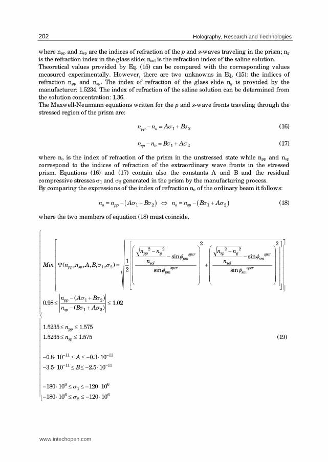
202

where npp and nsp are the indices of refraction of the p and s-waves traveling in the prism; ng

is the refraction index in the glass slide; nsol is the refraction index of the saline solution.

Theoretical values provided by Eq. (15) can be compared with the corresponding values

measured experimentally. However, there are two unknowns in Eq. (15): the indices of

refraction npp and nsp. The index of refraction of the glass slide ng is provided by the

manufacturer: 1.5234. The index of refraction of the saline solution can be determined from

the solution concentration: 1.36.

The Maxwell-Neumann equations written for the p and s-wave fronts traveling through the

stressed region of the prism are:

1 2pp on n A Bσ σ− = + (16)

1 2sp on n B Aσ σ− = + (17)

where no is the index of refraction of the prism in the unstressed state while npp and nsp

correspond to the indices of refraction of the extraordinary wave fronts in the stressed

prism. Equations (16) and (17) contain also the constants A and B and the residual

compressive stresses σ1 and σ2 generated in the prism by the manufacturing process.

By comparing the expressions of the index of refraction no of the ordinary beam it follows:

( )1 2o ppn n A Bσ σ= − + ⇔ ( )1 2o spn n B Aσ σ= − + (18)

where the two members of equation (18) must coincide.

2 2 2 2

1 2

1 2

1 2

2 2

sin sin1

( , , , , , )2 sin sin

( )0.98 1.0

( )

pp g sp gsper sperpm sm

sol solpp sp sper sper

pm sm

pp

sp

n n n n

n nMin n n A B

n A B

n B A

φ φσ σ φ φ

σ σσ σ

⎡ ⎤⎡ ⎤⎢ ⎥⎛ ⎞ ⎛ ⎞⎢ ⎥− −⎢ ⎥⎜ ⎟ ⎜ ⎟⎢ ⎥− −⎢ ⎥⎜ ⎟ ⎜ ⎟⎢ ⎥Ψ = +⎢ ⎥⎜ ⎟ ⎜ ⎟⎢ ⎥⎢ ⎥⎜ ⎟ ⎜ ⎟⎢ ⎥⎢ ⎥⎜ ⎟ ⎜ ⎟⎢ ⎥⎜ ⎟ ⎜ ⎟⎢ ⎥⎝ ⎠ ⎝ ⎠⎢ ⎥⎣ ⎦⎢ ⎥⎣ ⎦− +≤ ≤− +

11 11

11

2

1.5235 1.575

1.5235 1.575 (19)

0.8 10 0.3 10

3.5 10 2.

pp

sp

n

n

A

B

− −−

≤ ≤≤ ≤

− ⋅ ≤ ≤ − ⋅− ⋅ ≤ ≤ − 11

6 61

6 62

5 10

180 10 120 10

180 10 120 10

σσ

−

⎧⎪⎪⎪⎪⎪⎪⎪⎪⎪⎪⎪⎪⎪⎪⎨⎪⎪⎪⎪⎪⎪⎪⎪⎪ ⋅⎪⎪⎪− ⋅ ≤ ≤ − ⋅⎪⎪− ⋅ ≤ ≤ − ⋅⎩

www.intechopen.com


203

The optimization problem (19) was formulated where the objective function Ψ represents

the average difference between the theoretical angles at which the p and s-wave fronts

emerge in the saline solution and their counterpart measured experimentally. The Maxwell-

Neumann equations were included as constraints in the optimization process: the equality

constraint on the ordinary wave, Eq. (18), must be satisfied within 2% tolerance. There are

six optimization variables: the two indices of refraction npp and nsp in the error functional;

the two constants A and B and the residual stresses σ1 and σ2 in the constraint equation. The

last unknown of the optimization problem, the refraction index no corresponding to the

unstressed prism, can be removed from the vector of design variables by combing the

Maxwell-Neumann relationships into the constraint equation (18).

Three different optimization runs were carried out starting from: (i) lower bounds of design

variables (Run A); (ii) mean values of design variables (Run B); (iii) upper bounds of design

variables (Run C). The optimization problem (19) was solved by combining response surface

approximation and line search (Vanderplaats, 2001). SQP-MATLAB performed poorly as

design variables range over very different scales.

Fig. 9. Schematic of the optical path of p and s-polarized beams generated by the artificial

birefringence of prism.

Parameters Run A Run B Run C

npp 1.5447 1.5447 1.5468

nsp 1.5716 1.5709 1.5699

no 1.5399 1.5399 1.5405

A (m2/ N) −0.5167⋅10−11 −0.3017⋅10−11 −0.6994⋅10−11

B (m2/ N) −2.8096⋅10−11 −2.9645⋅10−11 −3.1390⋅10−11

C=A−B (m2/ N) 2.2929⋅10−11 2.6628⋅10−11 2.4396⋅10−11

σ1 (MPa) −135.30 −142.50 −161.85

σ2 (MPa) −145.01 −145.83 −164.90

τ (MPa) 4.8549 1.6657 1.5279

Residual error Ψ (%) 0.3872 0.2732 0.3394

Error on no (%) 1.730 1.673 1.485

Table 1. Results of optimization runs to analyze the effect of artificial birefringence of prism

www.intechopen.com


204

Optimization results are listed in Table 1. Besides the residual error on the optimized value

of Ψ and the constraint margin (18), the table shows also the resulting value of the index of

refraction of the ordinary beam no, the photoelastic constant C=A−B and the shear stress τ in

the prism determined as |(σ1−σ2)/ 2|. Remarkably, the residual error on emerging wave

angles is always smaller than 0.39%. The error on refraction index of the ordinary beam is

less than 1.75%. The optimization process was completed within 20 iterations.

6. Formation of the holograms at the nano-scale

The wave fronts emerging from the microscope slide play a role in the observation of the

prismatic NaCl nanocrystals contained in the saline solution. The observed images are not

images in the classical sense but they are lens holograms (theory of Fourier holography is

explained in the classical textbook written by Stroke (Stroke, 1969)) generated by the self-

luminous nanocrystals. Figure 10 shows the schematic representation of the optical circuit

bringing the images to the CCD detector. It can be seen that different diffraction orders

emerge from the interfaces of the crystals and the supporting microscope slide. These

emerging wave fronts act as multiplexers creating successive shifted images of the object.

Let us assume to look at a prism (Fig. 10, Part 1) approximately parallel to the image plane

of the CCD. Successive shifted luminous images of the prism are then recorded.

The largest fraction of energy is concentrated in the zero order and the first order

(Sciammarella et al., 2009). These orders overlap in an area that depends on the process of

formation of the image (see Fig. 10). The order 0 produces an image on the image plane of

the optical system, that is centered at a value x of the horizontal coordinate. Let us call S(x)

this image. The order +1 will create a shifted image of the particle, S(x-Δx). The shift implies

a change of the optical path between corresponding points of the surface. In the present

case, the trajectories of the beams inside the prismatic crystals are straight lines and the

resulting phase changes are proportional to the observed image shifts. The phase change is:

_ _( , ) ( ) ( )px x K S x S x xφ ⎡ ⎤Δ Δ = Δ⎣ ⎦ (20)

where Kp is a coefficient of proportionality. Equation (20) corresponds to a shift of the image

of the amount Δx. If the FT of the image is computed numerically, one can apply the shift

theorem of the Fourier transform. For a function f(x) shifted by the amount Δx, the Fourier

spectrum remains the same but the linear term ωspΔx is added to the phase: ωsp is the

angular frequency of the FT. It is necessary to evaluate this phase change. The shift can be

measured on the image by determining the number of pixels representing the displacement

between corresponding points of the image (see Fig. 10, Part 4). Through this analysis and

using the Fourier Transform it is possible to compute the thickness t of the prism in an

alternative way to the procedure that will be described in the following. These

developments are a verification of the mechanism of the formation of the images as well as

of the methods to determine prism thickness (Sciammarella et al., 2009).

Let us now consider the quasi-monochromatic coherent wave emitted by a nano-sized

prismatic crystal. The actual formation of the image is similar to a typical lens hologram of a

phase object illuminated by a phase grating (Tanner, 1974). The Fourier Transform of the

image of the nanocrystal extended to the complex plane is an analytical function. If the FT is

known in a region, then, by analytic continuation, F(ωsp) can be extended to the entire

domain. The resolution obtained in this process is determined by the frequency ωsp captured

www.intechopen.com


205

Fig. 10. Schematic representation of the optical system leading to the formation of lens

hologram: 1) Prismatic nanocrystal; 2) Wave fronts entering and emerging from the

polystyrene micro-sphere acting as a relay lens; 3) Wave fronts arriving at the focal plane of

the spherical lens; 4) Wave fronts arriving at the image plane of the CCD. The simulation of

the overlapping of orders 0, +1 and -1 in the image plane of the CCD is also shown.

in the image. The image can be reconstructed by a combination of phase retrieval and

suitable algorithms. The image can be reconstructed from a F(ωsp) such that ωsp<ωsp,max,

where ωsp,max is determined by the wave fronts captured by the sensor.

www.intechopen.com


206

The fringes generated by different diffraction orders experience phase changes that provide

depth information. These fringes are carrier fringes that can be utilized to extract optical

path changes. This type of setup to observe phase objects was used in phase hologram

interferometry as a variant of the original setup proposed by Burch and Gates(Burch et al.,

1966; Spencer and Anthony, 1968). When the index of refraction in the medium is constant,

the rays going through the object are straight lines. If a prismatic object is illuminated with a

beam normal to its surface, the optical path sop through the object is given by the integral:

( , ) ( , , )op is x y n x y z dz= ∫ (21)

where the direction of propagation of the illuminating beam is the z-coordinate and the

analyzed plane wave front is the plane x-y; ni(x,y,z) is the index of refraction of the object

through which light propagates.

The change experienced by the optical path is:

_

0( , ) ( , , )

t

op i os x y n x y z n dz⎡ ⎤Δ = ⎣ ⎦∫ (22)

where t is the thickness of the medium. By assuming that ni(x,y,z)=nc where nc is the index

of refraction of the observed nanocrystals, Eq. (22) then becomes:

Δsop(x,y) = (nc−no)t (23)

By transforming Eq. (23) into phase differences and making no=ns, where ns is the index of

refraction of the saline solution containing the nanocrystals, one can write:

2

( )c sn n tp

πφΔ = − (24)

where p is the pitch of the fringes present in the image and modulated by the thickness t of

the specimen. In general, the change of optical path is small and no fringes can be observed.

In order to solve this problem, carrier fringes can be added. An alternative procedure is the

introduction of a grating in the illumination path (Tanner, 1974). In the present case of the

nanocrystals, carrier fringes can be obtained from the FT of the lens hologram of analyzed

crystals. In the holography of transparent objects, one can start with recording an image

without the transparent object of interest. In a second stage, one can add the object and then

superimpose both holograms in order to detect the phase changes introduced by the object

of interest. In the present experiment, reference fringes can be obtained from the

background field away from the observed objects. This procedure presupposes that the

systems of carrier fringes are present in the field independently of the self-luminous objects.

This assumption is verified in the present case since one can observe fringes that are in the

background and enter the nanocrystals experiencing a shift.

7. Observation of prismatic sodium-chloride nanocrystals

The prismatic nanocrystals of sodium-chloride grow on the surface of the microscope slide

by precipitation from the saline solution. Different isomers of NaCl nanocrystals are formed

and they are the object of dimensional analysis. There is a variety of nano-isomers that can

form at room temperature (Hudgins et al., 1997). In this study, only three isomers types and

four crystals were analyzed out of a much larger population of possible configurations.

www.intechopen.com


207

Fig. 11. NaCl nanocrystal of length 54 nm: a) gray-level image (512 x 512 pixels); b) 3-D

distribution of light intensity; c) isophote lines; d) FT pattern; e) theoretical crystal structure.

Fig. 12. NaCl nanocrystal of length 55 nm: a) gray level image (512 x 512 pixels); b) 3-D


www.intechopen.com


208

The sodium-chloride nanocrystals are located in the recorded images by observing the

image of the lens hologram with increasing numerical zooming. A square region around a

selected particle is cropped and the image is digitally re-pixelated to either 512×512 pixels or

1024×1024 pixels to increase the numerical accuracy of the FT of the crystals images. Image

intensities are also normalized from 0 to 255. Figure 11 shows the nanocrystal referred to as

crystal L=54 nm. The isophotes (lines of equal light intensity) of the crystal along with the

corresponding isophote level lines and the FT of the image pattern are presented in the

figure; the theoretical structure of the nanocrystal is also shown.

A similar representation is given in Fig. 12 for another prismatic crystal with about the same

length, that will be referred as crystal L=55 nm.

Figure 13 illustrates the case of a square cross-section crystal that will be called crystal L=86

nm. Figure 13b is an image of the crystal recorded by a color camera; the crystal has a light

green tone. The monochromatic image and the color image have different pixel structures,

but, by using features of the images clearly identifiable, a correspondence between the

images could be established and the image of the nanocrystal located. The picture indicates

that the image color is the result of an electromagnetic resonance and not an emission of

light at the same wavelength as the impinging light wavelength.

Fig. 13. NaCl nanocrystal of length 86 nm: a) gray-level image (1024 x 1024 pixels); b) image

of the crystal captured by a color camera; c) 3-D distribution of light intensity; d) isophote

lines; e) FT pattern; f) theoretical crystal structure.

www.intechopen.com


209

Finally, Fig. 14 is relative to the nanocrystal referred to as crystal L=120 nm.

Fig. 14. NaCl nanocrystal of length 120 nm: a) gray-level image (512 x 512 pixels); b) 3-D


Since the change of phase is very small, fractional orders must be used for measuring the

change of optical path as the light travels through nanocrystals. The procedure to obtain

depth information from the recorded images is now described. For each analyzed crystal a

particular frequency is selected. This frequency must be present in the FT of the image and

should be such that the necessary operations for frequency separation are feasible. This

means that frequencies that do not depend on the thickness of the nanocrystal must not be

near the selected frequency. The frequency of interest is individualized in the background of

the observed object. Then, the selected frequency is located in the FT of the object. A proper

filter size is then selected to pass a number of harmonics around the chosen frequency.

Those additional frequencies carry the information of the change in phase produced by the

change of optical path. In the next step, the phase of the modulated carrier and the phase of

the unmodulated carrier are computed. The change of phase is introduced in Eq. (24) and

the value of t is computed. Since the phase difference is not constant throughout the

prismatic crystal face as it is unlikely that the crystal face is parallel to the image plane of

camera, an average thickness is computed. The process was repeated for all prismatic

crystals analyzed. For the nanocrystal L=86 nm, the face under observation is not a plane

but has a step; furthermore, the face is also inclined with respect to the CCD image plane.

Hence, depth was computed as an average of the depth coordinates of points of the face.

To completely describe the prisms, one needs to obtain the in-plane dimensions as well. For

that purpose, an edge detection technique based on the Sobel filter was utilized in this

www.intechopen.com


210

study. The edge detection is a difficult procedure since the Goos-Hänchen effect may cause

distortions of the wave fronts at the edges. However, a careful procedure allowed the edge

detection to be used within a margin of error of a few nanometers. It has to be expected that

the prismatic crystals faces are not exactly parallel to the image plane of the camera.

Furthermore, due to the integration effect of the pixels on the arriving wave fronts, not all

the nanocrystals images can provide meaningful results.

The values of thickness determined for the different nanocrystals were in good agreement

with the results provided by the image-shift procedure – Eq. (20) – outlined in Section 6: the

standard deviation is within ±5 nm.

Table 2 shows the experimentally measured aspect ratios of nanocrystal dimensions

compared with the corresponding theoretical values: the average error on aspect ratios is

4.59% while the corresponding standard deviation is ±6.57%.

Nanocrystal

length (nm)

Experimental dimensions

(nm)

Experimental

aspect ratio

Theoretical

aspect ratio

54 72 x 54 x 53 5.43 x 4.08 x 4 5 x 4 x 4

55 55 x 45 x 33.5 4.93 x 4.03 x 3 5 x 5 x 3

86 104 x 86 x 86 4.84 x 4 x 4 5 x 4 x 4

120 120 x 46 x 46 7.83 x 3 x 3 8 x 3 x 3

Table 2. Aspect ratio of the observed nanocrystals: experiments vs. theory

Table 3, on the basis of aspect ratios, shows the theoretical dimensions of the sides of

nanocrystals and compares them with the measured values: the average absolute error is

3.06 nm, the mean error is –1.39 nm, the standard deviation of absolute errors is ±3.69 nm. A

conservative assumption to estimate the accuracy of measurements is to adopt the smallest

dimensions of the crystals as given quantities from which the other dimensions are then

estimated. The smallest dimensions are the ones that have the largest absolute errors.

Nanocrystal

length (nm)

Dimensions

Measured

Dimensions

Theoretical

Difference

(nm)

72 66.3 +5.7

54 54 53 +1

53 53 -----

55 55.8 -0.8

55 45 55.8 -10.8

33.5 33.5 -----

104 107.5 -3.5

86 86 86 0

86 86 -----

120 122.7 -2.7

120 46 46 0

46 46 -----

Table 3. Main dimensions of the observed nanocrystals: experiments vs. theory.

www.intechopen.com


211

The theoretical structure 5×4×4 corresponding to the crystal L=86 nm has one step in the

depth dimension. The numerical reconstruction of this crystal is consistent with the

theoretical structure (Fig. 15a); Fig. 15c shows the level lines of the top face; Fig. 15d shows a

cross section where each horizontal line corresponds to five elementary cells of NaCl. The

crystal shows an inclination with respect to the camera plane that was corrected by means of

an infinitesimal rotation. This allowed the actual thickness jump in the upper face of the

crystal (see the theoretical structure in Fig. 15b) to be obtained. The jump in thickness is 26

nm out of a side length of 86 nm: this corresponds to a ratio of 0.313 which is very close to

theory. In fact, the theoretical structure predicted a vertical jump of one atomic distance vs.

three atomic distances in the transverse direction: that is, a ratio of 0.333.

Fig. 15. a) Numerical reconstruction of the NaCl nanocrystal of length 86 nm; b) theoretical

structure; c) level lines; d) rotated cross section of the upper face of the nanocrystal: the

spacing between dotted lines corresponds to the size of three elementary cells.

8. Observation of the polystyrene nanospheres

Microspheres and nanospheres made of transparent dielectric media are excellent optical

resonators. Unlike the NaCl nanocrystals whose resonant modes have not been previously

studied in the literature, both theoretical and experimental studies on the resonant modes of

microspheres and nanospheres can be found in the literature. Of particular interest are the

modes localized at the surface, along a thin equatorial ring. These modes are called

whispering-gallery modes (WGM). WGM result from light confinement due to total internal

reflection inside a high index spherical surface within a lower index medium and from

resonance as the light travels a round trip within the cavity with phase matching (Johnson,

1993). The WG modes are within the Mie’s family of solutions for resonant modes in light

scattering by dielectric spheres. The WG modes can also be derived from Maxwell equations

www.intechopen.com


212

by imposing adequate boundary conditions (Bohren and Huffman, 1998). They can also be

obtained as solutions of the Quantum Mechanics Schrodinger-like equation describing the

evolution of a complex angular-momentum of a particle in a potential well.

Figure 16a shows the image of a spherical particle of diameter 150 nm. This image presents

the typical WG intensity distribution. Waves are propagating around the diameter in

opposite directions thus producing a standing wave with 7 nodes and 6 maxima. The light is

trapped inside the particle and there is basically a surface wave that only penetrates a small

amount into the radial direction. The signal recorded for this particle is noisier compared

with the signal recorded for the prismatic crystals. The noise increase is probably due to the

Brownian motion of the spherical particles. While NaCl nanocrystals seem to grow attached

to the supporting surface, nanospheres are not in the same condition. Of all resonant

geometries a sphere has the capability of storing and confining energy in a small volume.

(a) (c)

(b)

Fig. 16. Spherical nanoparticle of estimated diameter 150 nm: a) FT and zero order filtered

pattern; b) systems of fringes modulated by the particle; c) color image of the particle.

The method of depth determination utilized for the nanocrystals can be applied also to the

nanospheres. While in prismatic bodies made out of plane surfaces the pattern

interpretation is straightforward, in the case of curved surfaces the analysis of the patterns is

more complex since light beams experience changes in trajectories determined by the laws

of refraction. In the case of a sphere the analysis of the patterns can be performed in a way

similar to what is done in the analysis of the Ronchi test for lens aberrations. Figure 16

shows the distortion of a grating of pitch p=83.4 nm as it goes through the nanosphere. The

appearance of the observed fringes is similar to that observed in a Ronchi test. The detailed

description of this process is not included in this chapter for the sake of brevity.

Figure 17a shows a spherical particle of estimated diameter 187 nm while Fig. 17b shows the

average intensity. Figure 17c is taken from Pack (2001) and shows the numerical solution for

the WGM of a polystyrene sphere of diameter 1.4 μm while Fig. 17d shows the average

intensity. There is good correspondence between experimental results and numerical

simulation. The electromagnetic resonance occurs at the wavelength λ=386 nm which

corresponds to UV radiation. The color camera is sensitive to this frequency and Fig. 16c

shows the color picture of the D=150 nm nanosphere: the observed color corresponds

approximately to the above mentioned resonance wavelength.

www.intechopen.com


213

(a) (b) (c) (d)

Fig. 17. Spherical nano-particle of estimated diameter 187 nm: a) Original image; b) Average

intensity image; c) Numerical simulation of WG modes; d) Average intensity of numerical

simulation.

Fig. 18. a) FT pattern of the image of the 150 nm polystyrene nanosphere; b) Fourier

transform of the real part of the FT of the nanosphere image; c) 2D view of the zero order

extracted from the real part of the FT pattern of the nanosphere image; d) cross-section of

the zero order in the X-direction; e) cross-section of the zero order in the Y-direction.

Four particles with radius ranging between 150 and 228 nm were analyzed. For example,

Fig. 18 illustrates the different stages involved by the determination of the D=150 nm

nanoparticle diameter. The Fourier transform of the image is shown in Fig. 18a while Fig.

18b shows the FT of the real part of the FT of the image. Figure 18c shows the intensity

distribution of order 0. Different peaks corresponding to fringe systems present in the image

can be observed. Figures 18d-e show the cross sections of the zero order with the

corresponding peaks observed in Fig. 18c. These patterns are similar to those observed for

the prismatic nanocrystals (Sciammarella et al., 2009). The gray level intensity decays from

255 to 20 within 75 nm: this quantity corresponds to the radius of the nanosphere.

An alternative way to determine diameter from experimental data is based on the WGM

properties that relate the diameter or radius of the nanosphere to the standing waves which

in turn are characterized by the number of zero nodes or the number of maxima. These

numbers depend on the index of refraction and on the radius of the nanosphere. The

numerical solution of the WG mode of polystyrene sphere developed by Pack (Pack, 2001)

www.intechopen.com


214

(a)

(b)

Fig. 19. Relationships between nanosphere radius and a) equatorial wavelength of the WG

mode; b) normalized equatorial wavelength of the WG mode.

was utilized in this study as the resonance modes occur approximately at the same

wavelength, λ=386 nm. Figure 19a shows the equatorial wave length of the WG plotted vs.

the particle radius. The experimentally measured wavelengths are plotted in a graph that

includes also the numerically computed value (radius of 700 nm). A very good correlation

(R2=0.9976) was obtained showing that the edge detection gradient utilized yields values

that are consistent with the numerically computed WG wavelengths. The graph shown in

Fig. 19b − the ratio of equatorial wavelength to radius is plotted vs. the radius − seems to

provide a correlation with a better sensitivity. The correlation was again good (R2=0.9994).

9. Summary and conclusions

This paper illustrated a new approach to investigations at the nano-scale based on the use of evanescent illumination. The proposed methodology allows to measure topography of

www.intechopen.com


215

nano-sized simple objects such as prismatic sodium-chloride crystals and spherical polystyrene particles. The basic foundation of the study is that the observed images are lens holographic interferograms of phase objects. The process of formation of those interferograms can be explained in view of the self-luminosity of the observed nano-objects caused by electromagnetic resonance. Another aspect to be considered is the possibility for the generated wave fronts to go through the whole process of image formation without the restrictions imposed by diffraction-limited optical instruments. Remarkably, nanometer resolution was achieved using an experimental setup including just a conventional optical microscope. Besides the nano-size objects, the diffraction pattern of a

6 μm microsphere illuminated by the evanescent field was also recorded by the sensor.

Although the sphere was in the range of the objects that can be visualized by classical microscopy, the diffraction pattern was described by an expansion of the electromagnetic field in a series of Bessel functions and coincided with the typical pattern of a super-resolving pupil. This is again a consequence of electromagnetic resonance phenomena

taking place in regions with dimensions smaller than the wavelength of the light. A great deal of theoretical developments is required to substantiate the experimentally observed properties of the illumination resulting from evanescent waves. However, it can be said that, from the point of view of direct application of these properties, it is possible to access the nano-range utilizing far-field observations. The results presented in the paper indicate that evanescent illumination is the key to making Experimental Mechanics methodologies well suitable for nano-engineering applications.

10. References

Ayyagari, R.S. and Nair, S. (2009). Scattering of P-polarized evanescent waves by a spherical dielectric particle. Journal of the Optical Society of America, Part B: Optical Physics, Vol. 26, pp. 2054-2058.

Bohren, C.F. and Huffman, D.R. (1998). Absorption and Scattering of Light by Small Particles. Wiley, New York (USA), ISBN: 978-0471293408.

Born, M. and Wolf, E. (1999). Principles of Optics. VII Edition. Cambridge University Press, Cambridge (UK), ISBN: 978-0521642224.

Bouchal, Z. (2003). Non diffracting optical beams: physical properties, experiments, and applications. Czechoslovak Journal of Physics, Vol. 53, pp. 537-578.

Brillouin, L. (1930). Les électrons dans les métaux et le classement des ondes de de Broglie correspondantes. Comptes Rendus Hebdomadaires des Séances de l'Académie des

Sciences, Vol. 191, pp. 292-294. Burch, J.W., Gates, C., Hall, R.G.N. & Tanner, L.H. (1966). Holography with a scatter-plate as

a beam splitter and a pulsed ruby laser as light source. Nature, Vol. 212, pp. 1347-1348, 1966.

Durnin, J., Miceley, J.J. & Eberli, J.H. (1987). Diffraction free beams. Physical Review Letters, Vol. 58, pp. 1499-1501.

General Stress Optics Inc. (2008) Holo-Moiré Strain Analyzer Version 2.0, Chicago (IL), USA. http:/ / www.stressoptics.com

Guillemet, C. (1970) L’interférométrie à ondes multiples appliquée à détermination de la répartition

de l’indice de réfraction dans un milieu stratifié. Ph.D. Dissertation, University of Paris, Paris (France).

Gutiérrez-Vega, J.C., Iturbe-Castillo, M.D., Ramirez, G.A., Tepichin, E., Rodriguez-Dagnino, R.M., Chávez-Cerda, S. & New, G.H.C. (2001). Experimental demonstration of optical Mathieu beams. Optics Communications, Vol. 195, pp. 35-40.

www.intechopen.com


216

Hernandez-Aranda, R.I., Guizar-Sicairos, M. & Bandres, M.A. (2006). Propagation of

generalized vector Helmholtz–Gauss beams through paraxial optical systems.

Optics Express, Vol. 14, pp. 8974–8988.

Hudgins, R.R., Dugourd, P., Tenenbaum, J.N. & Jarrold, M.F. (1997). Structural transitions

of sodium nanocrystals. Physical Review Letters, Vol. 78, pp. 4213-4216.

Jackson, J.D. (2001). Classical Electrodynamics, Third Edition. John Wiley & Sons, New York

(USA), ISBN: 978-0471309321.

Johnson, B.R. (1993). Theory of morphology-dependent resonances - shape resonances and

width formulas. Journal of the Optical Society of America, Part A: Optics Image Science

and Vision, Vol. 10, pp. 343-352.

Mugnai, D., Ranfagni, A. & Ruggeri, R. (2001). Pupils with super-resolution. Physics Letters,

Vol. A 311, pp. 77-81.

Mugnai, D., Ranfagni, A. & Ruggeri, R. (2004). Beyond the diffraction limit: Super-resolving

pupils. Journal of Applied Physics, Vol. 95, pp. 2217-2222.

Pack, A. (2001). Current Topics in Nano-Optics. PhD Dissertation. Chemnitz Technical

University, Chemnitz (Germany).

Sciammarella, C.A. (2008). Experimental mechanics at the nanometric level. Strain, Vol. 44,

pp. 3-19.

Sciammarella, C.A. and Lamberti, L. (2007). Observation of fundamental variables of optical

techniques in nanometric range. In: Experimental Analysis of Nano and Engineering

Materials and Structures (E.E. Gdoutos Ed.). Springer, Dordrecht (The Netherlands),

ISBN: 978-1402062384.

Sciammarella, C.A., Lamberti, L. & Sciammarella, F.M (2009). The equivalent of Fourier

holography at the nanoscale. Experimental Mechanics , Vol. 49, pp. 747-773.

Sciammarella, C.A., Lamberti, L. & Sciammarella, F.M. (2010). Light generation at the nano

scale, key to interferometry at the nano scale. Proceedings of 2010 SEM Annual

Conference & Exposition on Experimental and Applied Mechanics. Indianapolis (USA),

June 2010.

Spencer, R.C. and Anthony, S.A. (1968). Real time holographic moiré patterns for flow

visualization. Applied Optics, Vol. 7, p. 561.

Stroke, G.W. (1969). An Introduction to Coherent Optics and Holography, 2nd Edition. Academic

Press, New York (USA), ISBN: 978-0126739565.

Tanner, L.H. (1974). The scope and limitations of three-dimensional holography of phase

objects. Journal of Scientific Instruments, Vol. 7, pp. 774-776.

The MathWorks Inc. MATLAB® Version 7.0, Austin (TX), USA, 2006.

http:/ / www.mathworks.com

Toraldo di Francia, G. (1952). Super-gain antennas and optical resolving power. Nuovo

Cimento, Vol. S9, pp. 426-435.

Toraldo di Francia, G. (1958). La Diffrazione della Luce. Edizioni Scientifiche Einaudi, Torino

(Italy).

Vanderplaats, G.N. (2001). Numerical Optimization Techniques for Engineering Design, 3rd Edn.

VR&D Inc., Colorado Springs (USA), 2001, ISBN: 978-0944956014.

Vigoureux, J.M. (2003). De l’onde évanescente de Fresnel au champ proche optique. Annales

de la Fondation Luis de Broglie, Vol. 28, pp. 525-547.

Yu, F.T.S. (2000). Entropy and Information Optics. Marcel Dekker, New York (USA), ISBN:

978-0824703639.

www.intechopen.com

Holography, Research and TechnologiesEdited by Prof. Joseph Rosen

ISBN 978-953-307-227-2Hard cover, 454 pagesPublisher InTechPublished online 28, February, 2011Published in print edition February, 2011

InTech EuropeUniversity Campus STeP Ri Slavka Krautzeka 83/A 51000 Rijeka, Croatia Phone: +385 (51) 770 447 Fax: +385 (51) 686 166www.intechopen.com

InTech ChinaUnit 405, Office Block, Hotel Equatorial Shanghai No.65, Yan An Road (West), Shanghai, 200040, China

Phone: +86-21-62489820 Fax: +86-21-62489821

Holography has recently become a field of much interest because of the many new applications implementedby various holographic techniques. This book is a collection of 22 excellent chapters written by various experts,and it covers various aspects of holography. The chapters of the book are organized in six sections, startingwith theory, continuing with materials, techniques, applications as well as digital algorithms, and finally endingwith non-optical holograms. The book contains recent outputs from researches belonging to different researchgroups worldwide, providing a rich diversity of approaches to the topic of holography.

How to referenceIn order to correctly reference this scholarly work, feel free to copy and paste the following:

Cesar A. Sciammarella, Luciano Lamberti and Federico M. Sciammarella (2011). Optical HolographyReconstruction of Nano-objects, Holography, Research and Technologies, Prof. Joseph Rosen (Ed.), ISBN:978-953-307-227-2, InTech, Available from: http://www.intechopen.com/books/holography-research-and-technologies/optical-holography-reconstruction-of-nano-objects

© 2011 The Author(s). Licensee IntechOpen. This chapter is distributedunder the terms of the Creative Commons Attribution-NonCommercial-ShareAlike-3.0 License, which permits use, distribution and reproduction fornon-commercial purposes, provided the original is properly cited andderivative works building on this content are distributed under the samelicense.

https://creativecommons.org/licenses/by-nc-sa/3.0/

Optical Holography Reconstruction of...

Documents

Transcript of Optical Holography Reconstruction of...