One-sample inference: Categorical...

IntroductionConfidence intervals

Hypothesis testsConclusion

One-sample inference: Categorical Data

Patrick Breheny

October 8

Patrick Breheny STA 580: Biostatistics I



One-sample vs. two-sample studies

A common research design is to obtain two groups of peopleand look for differences between them

We will learn how to analyze these types of two-group, ortwo-sample studies in a few weeks

We are going to start, however, with a simpler case: theone-sample study




One-sample inference

For example, a researcher collects a random sample ofindividuals, measures their heights, and wants to make ageneralization about the heights in the population

Or a researcher collects a random sample of individuals,determines whether or not they smoke, and wants to makeinferences about the percentage of the population that smokes

These are examples of one-sample inference problems – thefirst involving continuous data, the second involvingcategorical data




One-sample inference: categorical data

Today’s topic is inference for one-sample categorical data

The object of such inference is percentages:

What percent of patients survive surgery?What percent of women develop breast cancer?What percent of people who do better on one therapy thananother?

Investigators see one percentage in their sample, but whatdoes that tell them about the population percentage?

In short, how accurate are percentages?




Approximate approachExact approachThe big picture

The normal approximation

A percentage is a kind of average – the average number oftimes an event occurs per opportunity

Thus, one approach is to use the central limit theorem, whichtells us that:

The expected value of the sample percentage is the populationpercentageThe standard error of the sample average is equal to thepopulation standard deviation divided by the square root of nThe shape of the sampling distribution is approximately normal(how accurate this is depends on n)





The normal approximation (cont’d)

Statisticians often use p to represent the populationproportion, and p̂ to represent the sample proportion

Thus, if we observe p̂ in our sample, the central limit theoremsuggests that p̂ is a good estimate of p

If p̂ is a good estimate of the population percentage, then itfollows that

√p̂(1− p̂) is a good estimate of the population

standard deviation

Continuing, a good estimate for the SE is

SE =

√p̂(1− p̂)

n





The probability that p and p̂ are close

If the probability that p̂ is within 1 standard error of p is 68%,what is the probability that p is within 1 standard error of p̂?

Also 68%; it’s the same thing, just worded differently

Therefore, if p plus or minus 1.96 standard errors has a 95%chance of containing p̂, then p̂ plus or minus 1.96 standarderrors has a 95% chance of containing p





The form of confidence intervals

Thus, x% confidence intervals look like:

(p̂− zx%SE, p̂+ zx%SE)

where zx% contains the middle x% of the standard normaldistribution

For 95% confidence intervals, then, z is always 1.96





Procedure for finding confidence intervals

To sum up, the central limit theorem tells us that we cancreate x% confidence intervals by:

#1 Calculate the standard error: SE =√p̂(1− p̂)/n

#2 Determine the values of the normal distribution that containthe middle x% of the data; denote these values ±zx%

#3 Calculate the confidence interval:

(p̂− zx%SE, p̂+ zx%SE)





Example: Survival of premature infants

In order to estimate the survival chances of infants bornprematurely, researchers at Johns Hopkins surveyed therecords of all premature babies born at their hospital in athree-year period

They found 39 babies who were born at 25 weeks gestation,31 of which survived at least 6 months

Their best estimate (point estimate) is that 31/39 = 79.5% ofall babies (in other hospitals, in future years) born at 25 weeksgestation would survive at least 6 months, but how accurate isthat percentage?





Example: Survival of premature infants (cont’d)

The standard error of the percentage is

SE =

√.795(1− .795)

39= 0.0647

So, one way of expressing the accuracy of the estimatedpercentage is: 79.5%± 6.5% (this would be about a 68%confidence interval)

Another way wold be to calculate the 95% confidence interval:

(79.5− 1.96(6.47), 79.5 + 1.96(6.47)) = (66.8%, 92.2%)





Problems with the normal approximation

That approach works pretty well, but if you think about it, thedistribution our data isn’t normal – it’s binomialThe normal approximation works because the binomialdistribution looks a lot like the normal distribution when n islarge and p isn’t close to 0 or 1Other times, the normal approximation doesn’t work as well

20 22 24 26 28 30 32 34 36 38

n=39, p=0.8

Pro

babi

lity

0.00

0.05

0.10

0.15

10 11 12 13 14 15

n=15, p=0.95

Pro

babi

lity

0.0

0.1

0.2

0.3

0.4





Example: Survival of premature infants, part II

In their study, the Johns Hopkins researchers also found 29infants born at 22 weeks gestation, none of which survived 6months

The normal approximation is clearly not going to work here,for two reasons:

The estimated standard deviation will be 0Even if it wasn’t, the confidence interval will be symmetricabout 0, so half of it would be negative





Using the binomial distribution directly

But why settle for an approximation?

The number of infants who survive is going to follow abinomial distribution; why not use that directly?

It seems pretty obvious that the lower limit of our confidenceinterval should be 0, but how can we use the binomialdistribution to find an upper limit?

The upper limit should be a number p such that there wouldonly be a 2.5% probability of observing 0 infants who surviveif the probability of surviving really were p





Finding the upper limit for p

0.00 0.05 0.10 0.15 0.20 0.25

0.0

0.2

0.4

0.6

0.8

1.0

p

P(0

out

of 2

9 in

fant

s su

rviv

e)





Exact confidence intervals

Thus, the exact confidence interval for the populationpercentage of infants who survive after being born at 22weeks is (0%,11.9%)

The exact confidence interval for the population percentage ofinfants who survive after being born at 25 weeks is(63.5%,90.7%)

Recall that our approximate confidence interval for thepopulation percentage of infants who survive after being bornat 25 weeks was (66.8%, 92.2%)





Exact vs. approximate intervals

When n is large and p isn’t close to 0 or 1, it doesn’t reallymatter whether you choose the approximate or the exactapproach

The advantage of the approximate approach is that it’s easyto do by hand

In comparison, finding exact confidence intervals by hand isquite time-consuming





Exact vs. approximate intervals (cont’d)

However, we live in an era with computers, which do the workof finding confidence intervals instantly (as we will see in lab)

If we can obtain the exact answer easily, there is no reason tosettle for the approximate answer

That said, in practice, people use and report the approximateapproach all the time

Possibly, this is because the analyst knew it wouldn’t matter,but more likely, it’s because the analyst learned theapproximate approach in their introductory statistics courseand doesn’t know any other way to calculate a confidenceinterval




Paired samplesThe sign testThe z-test

One-sample hypothesis tests

It is relatively rare to have specific hypotheses aboutpopulation percentages

One important exception is the collection of paired samples

In a paired sampling design, we collect n pairs of observationsand analyze the difference between the pairs





Hypothetical example: A sunblock study

Suppose we are conducting a study investigating whethersunblock A is better than sunblock B at preventing sunburns

The first design that comes to mind is probably to randomlyassign sunblock A to one group and sunblock B to a differentgroup

This is nothing wrong with this design, but we can do better





Signal and noise

Generally speaking, our ability to make generalizations aboutthe population depends on two factors: signal and noise

Signal is the magnitude of the difference between the twogroups – in the present context, how much better onesunblock is than the other

Noise is the variability present in the outcome from all othersources besides the one you’re interested in – in the sunblockexperiment, this would include factors like how sunny the daywas, how much time the person spent outside, how easily theperson burns, etc.

Hypothesis tests depend on the ratio of signal to noise – howeasily we can distinguish the treatment effect from all othersources of variability





Signal to noise ratio

To get a larger signal-to-noise ratio, we must either increasethe signal or reduce the variability

The signal is usually determined by nature and out of ourcontrol

Instead, we are going to have to reduce the variability/noise

If our sunblock experiment were controlled, we could attemptsuch steps as forcing all participants to spend an equalamount of time outside, on the same day, in an equally sunnyarea, etc.





Person-to-person variability

But what can be done about person-to-person variability (howeasily certain people burn)?

A powerful technique for reducing person-to-person variabilityis pairing

For each person, we can apply sunblock A to one of theirarms, and sunblock B to the other arm, and as an outcome,look at the difference between the two arms

In this experiment, the items that we randomly sample fromthe population are pairs of arms belonging to the same person





Benefits of paired designs

What do we gain from this?

As variability goes down,

Confidence intervals become narrowerHypothesis tests become more powerful

How much narrower? How much more powerful?

This depends on the fraction of the total variability thatcomes from person-to-person variability





More examples

Investigators have come up with all kinds of clever ways to usepairing to cut down on variability:

Before-and-after studies

Crossover studies

Split-plot experiments





Pairing in observational studies

Pairing is also widely used in observational studies

Twin studiesMatched studies

In a matched study, the investigator will pair up (“match”)subjects on the basis of variables such as age, sex, or race,then analyze the difference between the pairs

In addition to increasing power, pairing in observationalstudies also eliminates (some of the) potential confoundingvariables





Cystic fibrosis experiment

You may not have known it at the time, but you have alreadyconducted an exact hypothesis test for paired categorical datain your homework

Recall our cystic fibrosis experiment in which each patienttook both drug and placebo and the reduction in their lungfunction (measured by FVC) over a 25-week period wasrecorded

This is a crossover study, an example of a paired design





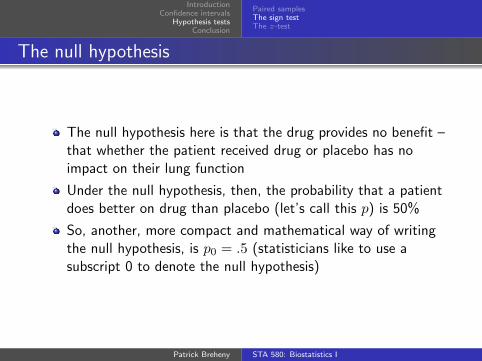
The null hypothesis

The null hypothesis here is that the drug provides no benefit –that whether the patient received drug or placebo has noimpact on their lung function

Under the null hypothesis, then, the probability that a patientdoes better on drug than placebo (let’s call this p) is 50%

So, another, more compact and mathematical way of writingthe null hypothesis, is p0 = .5 (statisticians like to use asubscript 0 to denote the null hypothesis)





The sign test

We can test this null hypothesis by using our knowledge that,under the null hypothesis, the number of patients who dobetter on the drug than placebo (x) will follow a binomialdistribution with n = 14 and p = 0.5This approach to hypothesis testing is called the sign test

All we need to do is calculate the p-value (the probability ofobtaining results as extreme or more extreme than the oneobserved in the data, given that the null hypothesis is true)





“As extreme or more extreme”

The result observed in the data was that 11 patients didbetter on the drug

But what exactly is meant by “as extreme or more extreme”than 11?

It is uncontroversial that 11, 12, 13, and 14 are as extreme ormore extreme than 11

But what about 0? Is that more extreme than 11?

Under the null, P (11) = 2.2%, while P (0) = .006%So 0 is more extreme than 11, but in a different direction





One-sided vs. two-sided tests

Potentially, then, we have two different approaches tocalculating this p-value:

Find the probability that x ≥ 11Find the probability that x ≥ 11 ∪ x ≤ 3 (the number that isas far away from the expected value of 7 as 11 is, but in theother direction)

These are both reasonable things to do, and intelligent peoplehave argued both sides of the debate

However, the statistical and scientific community has for themost part come down in favor of the latter – the so called“two-sided test”

For this class, all of our tests will be two-sided tests





The sign test

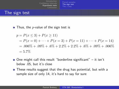
Thus, the p-value of the sign test is

p = P (x ≤ 3) + P (x ≥ 11)= P (x = 0) + · · ·+ P (x = 3) + P (x = 11) + · · ·+ P (x = 14)= .006% + .09% + .6% + 2.2% + 2.2% + .6% + .09% + .006%= 5.7%

One might call this result “borderline significant” – it isn’tbelow .05, but it’s close

These results suggest that the drug has potential, but with asample size of only 14, it’s hard to say for sure





Introduction

Thinking about the sign test, what enabled us to calculate thep-value? How were we able to attach a specific number to theprobability that x would take on certain values?

We were able to do this because we knew that, under the null,x followed a specific distribution (in that case, the binomial)

This is the most common strategy for developing hypothesistests – to calculate from the data a quantity for which weknow its distribution under the null hypothesis

Note that in general, we would not know the distribution ofthe number of patients who do better on drug than placebo –only under the null hypothesis





Test statistics

This quantity that we know the distribution of under the nullhypothesis is called a test statistic

Because we can calculate the test statistic from the data, andbecause we know its distribution under the null hypothesis, wecan calculate the probability of obtaining a result as extremeor more extreme than the observed result (the p-value)





The z test statistic

As we did before with confidence intervals, we can use thecentral limit theorem for this problem, now to create a teststatistic

From the central limit theorem, we know that z, the numberof standard errors away from p that p̂ falls, follows(approximately) a standard normal distribution

Our test statistic, then is

z =p̂− p0

SE

Having calculated z, we can get p-values from the standardnormal distribution

This approach to hypothesis testing is called the z-test





The standard error

What about the standard error?

Under the null, the population standard deviation is√p0(1− p0), which means that, under the null,

SE =

√p0(1− p0)

n





Procedure for a z-test

The procedure for a z-test is then:

#1 Calculate the standard error: SE =√p0(1− p0)/n

#2 Calculate the test statistic z = (p̂− p0)/SE#3 Calculate the area under the normal curve outside ±z





The z-test for the cystic fibrosis experiment

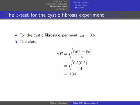
For the cystic fibrosis experiment, p0 = 0.5Therefore,

SE =

√p0(1− p0)

n

=

√0.5(0.5)

14= .134





The z-test for the cystic fibrosis experiment (cont’d)

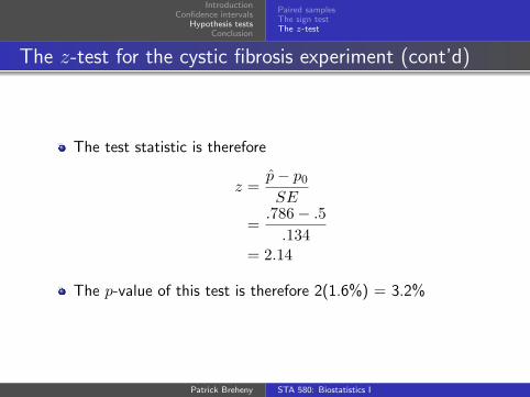
The test statistic is therefore

z =p̂− p0

SE

=.786− .5.134

= 2.14

The p-value of this test is therefore 2(1.6%) = 3.2%




Confidence intervals can produce hypothesis tests

It may not be obvious, but there is a close connection betweenconfidence intervals and hypothesis tests

For example, suppose our hypothesis test was to construct a95% confidence interval and then reject the null hypothesis ifp0 was outside the interval

It turns out that this is exactly the same as conducting ahypothesis test with α = 5%




Hypothesis tests can produce confidence intervals

Alternatively, suppose we formed a collection of all the valuesof p0 for which the p-value of our hypothesis test was above5%

This would form a 95% confidence interval for p

Note, then, that there is a correspondence between hypothesistesting at significance level α and confidence intervals withconfidence level 1− αIt turns out that the z-test corresponds to the approximateinterval, and that the sign test corresponds to the exactinterval




Conclusion

In general, then, confidence levels and hypothesis tests alwayslead to the same conclusion

This is a good thing – it would be confusing otherwise

Furthermore, this is not just true of confidence intervals forone-sample categorical data; it is generally true of allconfidence intervals and hypothesis tests

However, the information provided by each technique isdifferent: the confidence interval is an attempt to estimate aparameter, while the hypothesis test is an attempt to measurethe evidence against the hypothesis that the parameter isequal to a certain, specific number


One-sample inference: Categorical...

Documents

Transcript of One-sample inference: Categorical...