On the use of density kernels for concentration estimations within particle and puff dispersion...

*E-mail: [email protected].

Atmospheric Environment 33 (1999) 2007—2021

On the use of density kernels for concentration estimationswithin particle and puff dispersion models

Peter de Haan*

Swiss Federal Institute of Technology, GIETH, Winterthurerstrasse 190, 8057 Zurich, Switzerland

Received 7 May 1998; received in revised form 27 November 1998; accepted 27 November 1998

Abstract

Stochastic particle models are the state-of-science method for modelling atmospheric dispersion. They simulate thereleased pollutant by a large number of particles. In most particle models the concentrations are estimated by countingthe number of particles in a rectangular volume (box counting). The effects of the choice of the width and of the positionof these boxes on the estimated concentration is investigated. For the estimation of the concentration at a given point inspace, it is shown that this numerical procedure can cause either oversmoothed predictions or too much scatter. As analternative approach, the density kernel method to estimate concentrations is proposed, which optimizes bias andvariance. It allows for a reduction of the number of particles simulated for the same accuracy. The efficiency of severaldensity kernel shapes is compared, and methods for choosing their bandwidths are proposed. The relationship betweenthe numerically motivated bandwidths and the description of the growth of a cluster of pollutant particles (puffdispersion) is discussed. ( 1999 Elsevier Science Ltd. All rights reserved.

Keywords: Kernel density estimation; Box counting; Particle models; Puff models; Relative diffusion

1. Introduction

At present, stochastic particle or random-walk modelsare the most advanced approach to simulate atmosphericdispersion, especially for convective atmospheric condi-tions (for a review, see Wilson and Sawford, 1996). Insuch particle models, the emitted pollutant is simulatedby a large number of particles, which are assumed toexactly follow the flow. This approach has several ad-vantages over dispersion models like Gaussian plume orpuff models. However, simulating the emitted pollutantby many discrete particles brings up one difficulty: the cor-rect estimation of the concentration at a certain location.

In atmospheric dispersion modelling with stochasticparticle models, it is a common practice to calculate suchaverages over a grid cell in space, i.e. by counting allparticles in a box (see, for example, Borgas and Sawford,1994; Luhar and Rao, 1994; Hurley and Physick, 1991;Luhar and Britter, 1989; Rotach et al., 1996). The estima-tion of concentration is then obtained by multiplying thenumber of particles with their mass, and dividing thistotal mass by the size of the grid box. This way ofcounting the number of particles in a box is identical tocalculating a three-dimensional histogram. Of course, ifthe volume average over such a box is what the modellerwants, such box-counting methods are most efficient.

Histogram estimations in general depend, however, onthe choice of the width and the centre of the averaginginterval, area or volume. To estimate point concentra-tions in the context of atmospheric dispersion modelling,

1352-2310/99/$ - see front matter ( 1999 Elsevier Science Ltd. All rights reserved.PII: S 1 3 5 2 - 2 3 1 0 ( 9 8 ) 0 0 4 2 4 - 5

there are no physical restrictions determining either thecentre of a numerical averaging volume, or its size (be-sides the sampling volume of field instruments, whichwould lead to very small averaging volumes). This meansthat when choosing large averaging volumes, importantdetails might get lost, and the estimation of the con-centration density simulated by the particles will beoversmoothed. On the other hand, when choosing smallaveraging volumes, one runs at risk having random fluc-tuations in the number of particles per sampling volume.The stochastic particle modeller will thus try to choose‘‘reasonable’’ sizes and positions of the averaging vol-umes. The differences in the resulting concentration pre-dictions can be significant (see Section 2) and of the sameorder of magnitude as effects which are of interest (i.e. areto be modelled). It should be stressed that this uncertain-ty originates from a numerical procedure only. Sinceatmospheric dispersion modelling already has to copewith considerable uncertainties, it is desirable to havea numerical method for concentration estimation withinparticle models which does not lead to much additionaluncertainty.

Another approach to obtain concentrations withstochastic particle models is the backward-modelling ap-proach of Flesch et al. (1995). In this approach boxcounting is used, but instead of having an exact sourcelocation, the backward method has an exact receptorposition (and thus sampling box position), and all back-ward trajectories coming ‘‘near’’ to (i.e. originating from)the source are related to that source. This approach issuited for area sources together with small receptor vol-umes. But even then, in principle the uncertainties relatedwith either box counting or kernel methods can only becircumvented when the source is located exactly atground level, and all particles being reflected at theground surface within the source area being related to thesource. Flesch et al. (1995) discuss this special case indetail.

Clearly, for very high particle densities, the uncertain-ties of box counting vanish; e.g. Borgas and Sawford(1994) theoretically assume the number of particles be‘‘high enough’’ for the choice of the dimensions of theparticle counting box to be ‘‘negligible’’. But at present,computing power still drastically limits the number ofparticles which are normally emitted. With computingpower currently available, only for one-dimensionalmodels the effects might become negligible (see Section 2).

For these reasons, another method is proposed in thispaper. It relies on the concept of density distributions ofdifferent shape which are ‘‘added’’ to the particle’s posi-tion, i.e. the mass represented by the particle is spread outin space. Such a density distribution around the centre ofmass is called the density kernel. The kernel method hasbeen widely applied since it was introduced in 1950 (fora good review, see Scott 1992, Ch. 6), whereas in atmo-spheric dispersion modelling the box counting method is

still used despite its deficiencies; Lorimer (1986) was thefirst, to the author’s knowledge, to use a kernel methodfor atmospheric dispersion modelling.

In contrary to the choice of box size and position,which makes the box counts a bad choice for concentra-tion estimation, the shape of the kernel and its width asa function of the particle distribution have to be specified.Of these two, the latter is chosen such that the bias andvariance of the concentration estimation are minimisedjointly. The number of particles normally simulated atpresent is more than sufficient to let this method becomenearly independent of the shape of the kernel. This makesthe kernel density method a suitable approach for par-ticle modellers to estimate the concentrations simulatedby their model.

The RAPTAD model of Yamada et al. (1987) andYamada and Bunker (1988) combines a particle modelwith Gaussian-shaped density kernels. They use thephysical concept of absolute dispersion to estimate theappropriate size of these kernels. This approach is dis-cussed in more detail in Section 6.

The box counting method to estimate concentrationsin particle models is reviewed in Section 2. The concept ofdensity kernel estimators is introduced in Section 3, andthe important issue of the determination of the band-width of such kernels is treated in Section 4. Differentkernel shapes are compared in Section 5. The analogybetween these numerically determined density kernelsand the physical description of the expansion of a clusterof particles is discussed in Section 6.

2. Concentration estimation by box counting

2.1. Box counting in particle models

The smoothing of any given data actually is a non-parametric method to estimate the ‘‘true’’ curve (beinga density or a function), which is polluted by randomnoise. Most particle model simulations are one- or two-dimensional. The histogram (i.e. box counting, see above)still is the commonly used density estimator for particlemodels. In the vertical direction, the size of the intervals(the averaging volume) is often constant with height. Fortheir one-dimensional model, Luhar and Britter (1989)and Luhar et al. (1996), with 15 000 and 20 000 particlesreleased, respectively, use vertical box heights *z of*z/z

i" 0.05, and a ‘‘horizontal’’ extent *X"0.1, where

X is the dimensionless travel distance, X"w*t/zi, and

w* denotes the convective velocity scale. Luhar and Rao(1994) release 12 000 particles per hour in their fullythree-dimensional model, and use box dimensions*x]*y]*z of 200 m]50 m]10 m for elevated and200 m]25 m]5 m for surface releases (and take theaverage over 1 h). Hurley and Physick (1991) have 5000

2008 P. de Haan / Atmospheric Environment 33 (1999) 2007—2021

particles released in a two-dimensional model, and take*z"25 m (with the inversion height z

i"1000 m) and

*x"100 m. Rotach et al. (1996) present a two-dimen-sional model and use 10 000 particles; the dimensions ofthe averaging boxes are *z"20 m (with inversion heightvarying from 820 to 1980 m) and *x"300 m.

The amount of additional variability of the modelpredictions caused by the box counting method differs.For one-dimensional models and the use of approx.100000 particles, this variability seems to be small,whereas for two-dimensional particle models, this samenumber of particles, when applying Taylor’s frozen tur-bulence hypothesis, has to be simulated for far longertime periods, which is about the limit of today’s possibili-ties. For three-dimensional models, the order of magni-tude of the number of particles roughly is the square ofthe number used in one- and two-dimensional models.

For example, Venkatram and Du (1997) report thatwith the simulation of 50000 particles in a one-dimen-sional model, model results are not sensitive to the size ofthe numerical sampling box. On the other hand, Du andWilson (1994) (who do not mention the number ofsimulated particles) show concentration contour plotsfrom a two-dimensional model where the size of thesampling volume can still be detected from the figuresshown in their paper. The same holds for results from theone-dimensional particle model from Thomson andMontgomery (1994), who use 90000 to 120000 particles.This means that for two- and three-dimensional models,the expected increases in computing power in the nearfuture will not be sufficient to rely on box countingconcentration estimations. Anyway, all of the box sizesused by particle modellers mentioned above are averagesover volumes far larger than any receptor sampling vol-ume.

Also, Yamada and Bunker (1988) report that determin-ing the concentration at a given time and location bycounting the particles simulated by their fully three-di-mensional RAPTAD meso-scale particle model yieldsconsiderably varying results, depending on the size of thesampling volume and the number of particles used.

2.2. Near-source concentration estimation

Two areas can be identified where the box-countingmethod is most likely to be sensitive. Firstly, concentra-tion predictions for the near-source field, where changesin the particle density are sharp and large proportions ofthe total number of particles might still be within thevolume of few sampling boxes. Secondly, the estimationof surface concentrations, which are of interest for mostair pollution simulations, but are likely to show gradientsnear the surface over distances similar to the verticalextent of box sampling volumes. For concentrationpredictions in the far field and for smooth particle prob-ability density functions, the box-counting method will

produce the same results as any other method, althoughthe kernel method remains more efficient in these cases aswell.

As an example to illustrate the variability in concentra-tion predictions while using the box counting method,simulations have been performed for a non-buoyant re-lease at the height z

s"z

i/2, with different widths and

positions of the boxes in which the particles are counted(Fig. 1). For the simulation, 1000 particles are emitted persecond, the total duration of the simulation was 1000 s.The stochastic Lagrangian particle model used fulfils thewell-mixed condition of Thomson (1987). All details ofthe model are outlined in Rotach et al. (1996).

Concentration predictions for two sampling box sizesare shown in Fig. 1. The vertical size of 0.05z

i(dashed line

in Fig. 1) is often chosen by particle modellers (see above).The ‘‘true’’ concentration profile, based on 100 000 in-stead of 1000 particle trajectories, is depicted by a thickline in Fig. 1. It becomes clear that the near-sourcemaximum concentration will be clearly underestimatedfor box sizes of 0.05z

i. The other density estimation

shown in Fig. 1, with box size 0.005zi(short-dashed line),

makes the concentration prediction fluctuating from onebox volume to the other. However, the true value ofconcentration is approximated more adequately by thesmaller box sampling volumes, despite the additionalscatter. An additional smoothing procedure would im-prove the results (see, for example, Rotach et al., 1996). Asan example, the results from a kernel density estimationfollowing the recommendations of Section 5.5 of thispaper are also depicted in Fig. 1 (thin line).

2.3. Ground-level concentration estimations

In Fig. 2 an example for the effects of box counting onpredicting ground-level concentrations is given. In thisnumerical experiment, the release took place at a heightof 5 m, i.e. within the lowest sampling box. As for Fig. 1,results for vertical box sizes of 0.05z

i(dashed line) and

0.005zi

(dotted line) are depicted. Also shown are the‘‘true’’ concentration based on 100 000 particles (thickline) and the results from a triweight density kernel con-structed after Section 5.5 (thin line).

For the (widely used) 0.05zi

vertical box size, theground-level concentrations, in this example, are over-smoothed, i.e. underestimated, by a factor of appro-ximately 2 in the near-source field. The box size inthe horizontal directions has been chosen equal to thevertical box size, leading to a first box centre at a down-wind-distance of approx. 5 m (0.005z

ibox size) and 50 m

(0.05zibox size), respectively. For the smaller box with

0.005zivertical size, the estimates show a large random

scatter (large variance) but no bias. The kernel estima-tion, on the other hand, provides a smooth estimate withalmost no bias.

P. de Haan / Atmospheric Environment 33 (1999) 2007—2021 2009

Fig. 1. Vertical profiles of estimated concentration (in lgm~3) for different sizes of the boxes in which the particles are counted. Profilesare taken at 200, 300, 400, and 500 m downwind of the source. The dashed line (- - -) shows the box counting prediction for vertical andhorizontal box sizes of 0.05 z

i. The dotted line (- - -) is for vertical and horizontal sizes of 0.005z

i. The thick line (––) depicts the ‘‘true’’

concentration (see text). The thin solid line (—) shows the concentration predition using the kernel method as recommended in Section5.5. Release height is at z/z

i"0.5; source strength 1 g s~1; z

i"2000 m, u*"0.36 m s~1, ¸"!37 m, u6 (z "10 m)"2.1 m s~1.

3. Density kernels

3.1. Concentration estimation with density kernels

The kernel density estimator for the normalised con-centration c of n given particles of equal mass at positionsxiis

c(x) "1

nh

n+

i/1

KAx!x

ih B, (1)

where h is the width of the kernels (see Section 4), andK is the kernel function, fulfilling K(x)50 ∀x, andnormalised so that

: K(x) dx " 1 (2)

(thus making c a density distribution, i.e., :c(x) dx"1).One of the most widely used kernels is the Gaussian

kernel KG,

KG(r)"

1

(2n)d@2expA!

1

2rTrB, (3)

where d denotes the dimension (for example, d"2 fortwo-dimensional particle models).

The proper choice of the bandwidth h is of greaterimportance than the choice of the shape of the kernel(additional kernel shapes are introduced in Section 3.2),since h plays the role of a smoothing parameter. Thereare several proposals for determining the value of h fromthe data. These methods aim at ‘‘balancing’’ two counter-acting measures, the bias (caused by the smoothing,which increases for large h) and the variance (increasingfor small h).

In the following, the underlying distribution of particlepositions x

iwill be denoted as f (x). Then, the measure on


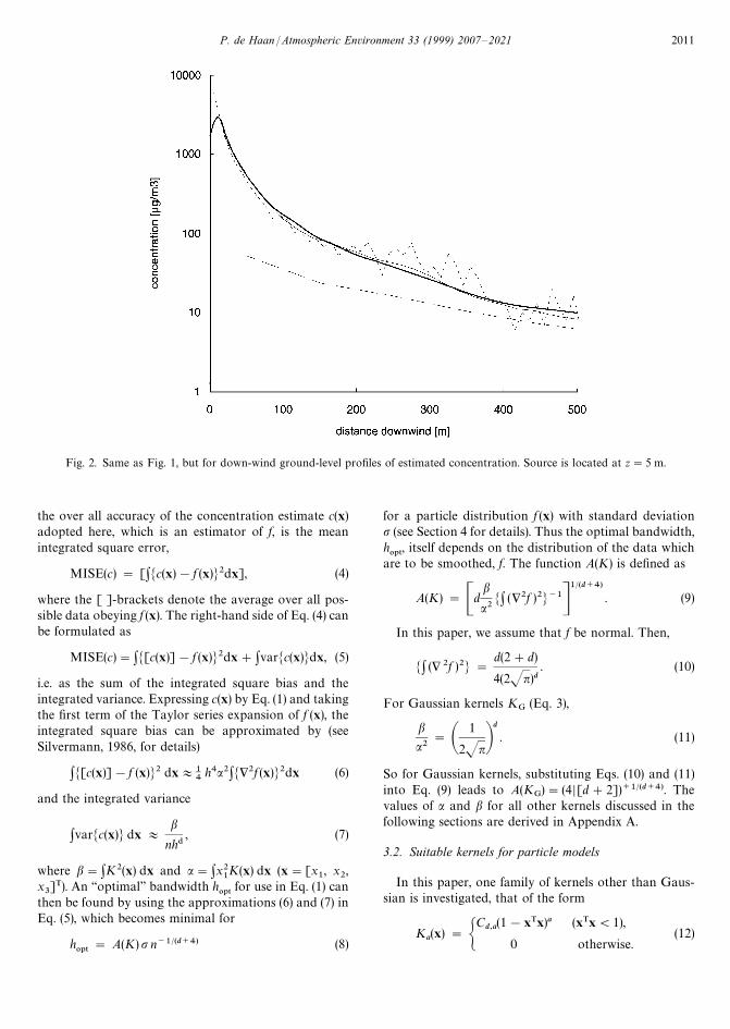
Fig. 2. Same as Fig. 1, but for down-wind ground-level profiles of estimated concentration. Source is located at z"5 m.

the over all accuracy of the concentration estimate c(x)adopted here, which is an estimator of f, is the meanintegrated square error,

MISE(c) " [:Mc(x)!f (x)N2dx], (4)

where the [ ]-brackets denote the average over all pos-sible data obeying f (x). The right-hand side of Eq. (4) canbe formulated as

MISE(c)":M[c(x)]!f (x)N2dx#:varMc(x)Ndx, (5)

i.e. as the sum of the integrated square bias and theintegrated variance. Expressing c(x) by Eq. (1) and takingthe first term of the Taylor series expansion of f (x), theintegrated square bias can be approximated by (seeSilvermann, 1986, for details)

:M[c(x)]!f (x)N2 dx+14

h4a2:M+2f (x)N2dx (6)

and the integrated variance

:varMc(x)N dx +

b

nh$, (7)

where b":K2(x) dx and a":x21K(x) dx (x"[x

1, x

2,

x3]T). An ‘‘optimal’’ bandwidth h

015for use in Eq. (1) can

then be found by using the approximations (6) and (7) inEq. (5), which becomes minimal for

h015

" A(K)p n~1@(d`4) (8)

for a particle distribution f (x) with standard deviationp (see Section 4 for details). Thus the optimal bandwidth,h015

, itself depends on the distribution of the data whichare to be smoothed, f. The function A(K) is defined as

A(K) " Cdb

a2M: (+2f )2N~1D

1@(d`4). (9)

In this paper, we assume that f be normal. Then,

M: (+ 2f )2N "

d(2#d)

4(2Jn)d. (10)

For Gaussian kernels KG

(Eq. 3),

ba2

" A1

2JnBd. (11)

So for Gaussian kernels, substituting Eqs. (10) and (11)into Eq. (9) leads to A(K

G)"(4 D[d#2])`1@(d`4). The

values of a and b for all other kernels discussed in thefollowing sections are derived in Appendix A.

3.2. Suitable kernels for particle models

In this paper, one family of kernels other than Gaus-sian is investigated, that of the form

Ka(x) " G

Cd,a

(1!xTx)a (xTx(1),

0 otherwise.(12)


Table 1Normalisation constant C

d,afor Epanechnikov (a"1), biweight

(a"2), triweight (a"3), quadweight (a"4) and quintweight(a"5) kernels for up to three dimensions (c

1"2, c

2"n,

c3"4n/3)

Cd,a

a"1 a"2 a"3 a"4 a"5

d"1 3 15 105 945 6932c

18c

148c

1384c

1256c

1d"2 2 3 4 5 6

c2

c2

c2

c2

c2

d"3 5 35 315 1155 30032c

38c

348c

3128c

3256c

3

Fig. 3. Comparison of one-dimensional Gaussian, Epanech-nikov, bi-, tri-, quad- and quintweight kernels. The bandwidth ofthe Gaussian kernel is unity, and taken from Table 2 for theother kernels (see Section 4.2). (Only the part for positive x isdepicted; all kernels are symmetric around zero.)

In Eq. (12), Cd,a

are normalising factors (Table 1) ensuringthat :K

adx"1, which are derived in Appendix A. For

a"1 up to a"5, these kernels are called Epanechnikovand bi-, tri, quad- and quintweight kernels, respectively.Fig. 3 depicts their one-dimensional form, with differentbandwidths h for every kernel. The relations betweenvalues of h for different kernels having approximately thesame smoothing effect are given in Section 4.2.

Note that the support (the d-dimensional interval overwhich the kernel function is non-zero) is infinite for theGaussian kernel (Eq. (3)) and limited for the other fivetypes (Eq. (12)). The Epanechnikov kernel (a"1) is opti-mal in minimising the MISE (Epanechnikov, 1969), butits derivative is discontinuous. As can be seen from Fig. 3,the differences between the Gaussian kernel and kernelsof the (1!xTx)a-type decrease for increasing a, the onlysignificant differences occurring at the tails of the distri-bution. Because of the small differences between thekernel shapes, other criteria such as the ease of computa-tion are important as well as the question, which of thekernel functions resembles most the distribution ofobserved turbulent wind fluctuations. The latter aregenerally assumed to be normally distributed (with theexception of the vertical component for convective condi-tions), making the Gaussian kernel the most naturalchoice. However, the assumption of a normal distribu-tion of wind fluctuations attributes a non-zero possibility(though very small) to unphysically large values. Thiswould support the choice of a kernel with a limitedsupport interval such as, say, the triweight kernel.

Another approach is the kernel method adopted byLorimer (1986). He uses the product of a three-dimen-sional Gaussian with a three-dimensional Epanechnikovkernel. Because this kernel is still defined over an infinitedomain, we only compare kernels after Eq. (12) with theGaussian kernel.

It should be kept in mind that the concentration es-timation using density kernels within particle models isa numerical task, and thus any form of kernel functioncan be used in principle. But the analogies which show up

between these numerically motivated kernel densityestimators and the concept of clusters of particles asadopted in puff models is remarkable, and is furtherdiscussed in Section 6. Recommended kernel functionswhich perform well numerically and have a form whichcan be compared to physical observations are given inSection 5.5.

3.3. Three-dimensional vs. product kernels

The approach formulated in Section 3.1 is d-dimen-sional, and thus yields a single bandwidth for d-dimen-sional kernels. Since atmospheric dispersion in thelogitudinal, cross-wind and vertical directions is, fromthe point of view of density estimation, very similar, thisapproach is justified.

In other scientific areas, however, often three-dimen-sional density kernels are being used which are the prod-uct of one-dimensional kernels. In such so-called productkernels, instead of Eq. (1),

c(x) "1

nhxhyhz

n+i/1G

3<j/1

KAxi!x

ijhjBH . (13)

where the bandwidths hiof the kernel distributions in the

three directions are calculated in analogy to the one-dimensional case. Product kernels have the advantage ofeasier mathematics, and are easier to handle in the case ofdata points with large differences in the standard devi-ations in the three directions (dimensions).


Fig. 4. Density differences for a two-dimensional triweight vs.the corresponding product kernel.

For Gaussian kernels, Eqs. (1) and (13) are identical.This relationship does not hold any longer for Eq. (12)-type kernels. Fig. 4 depicts the differences in densitydistribution between a three-dimensional triweight (usingEq. (1)) and the corresponding product kernel (Eq. (13)).The product kernel formulation leads to higher densitiesin the edges and in the centre of the carrier domain, whilehaving smaller densities in the other regions. In the fieldof atmospheric dispersion, diffusion is approximatelyequal in all directions and no ‘‘edges’’ with higher prob-abilities exist. This means that product kernels are lesssuited for atmospheric dispersion data than fully three-dimensional kernels. Therefore, only the latter are inves-tigated in this paper. But for applications where thestandard deviations of the data points substantially differaccording to direction, product kernels may avoid thenecessity of scale transformations.

4. Bandwidth estimation

4.1. Theory

The optimal bandwidth as given by Eq. (8) is onlyoptimal under the assumption that the distribution of thedata be normal. Therefore, more robust rules-of-thumbhave been constructed. A recommended one is

h30"

"aA(K) n~1@(d`4) minAp,R

1.34B , (14)

where R is the interquartile range, i.e. R"R3@4

!R1@4

,and a is taken as 0.85 in the present study. The upperquartile R

3@4and lower quartile R

1@4are defined as those

values out of the data to be smoothed where 25% of thedata has a larger or smaller value, respectively.

Lorimer (1986) used a slightly different approach todetermine the kernel bandwidth. The bandwidth for theinitial particle distribution was calibrated by visual com-parision of the resulting density distribution. This pro-vides an approximate value for the term A(K)n~1@(d`4) inEq. (14), which remains constant. Then, Lorimer (1986)calculates the new standard deviation of the particleensemble for every new time step, and thus calculates thebandwidth using Eq. (14).

At this point, the idea of having an estimate pL for thevalue of p might come up. This would circumvent tosome extent the fact that the optimal bandwidth dependson the density distribution of the particles to besmoothed, and would save computing time, as the stan-dard deviation of the given particle distribution has notto be calculated. However, deriving expressions forpL means to theoretically solve the problem of atmo-spheric dispersion, and then no numerical dispersionmodel would be required as soon as correct, i.e. bias-freepL expressions (as a function of travel time or of downwinddistance) are available.

4.2. Equivalent bandwidths for different kernels

It is possible to switch between kernels without recon-sidering the optimal bandwidth. As soon as an optimalbandwidth has been chosen for one type of kernel, band-widths for other kernels which show the same smoothingcharacteristics (called ‘‘equivalent bandwidths’’, can bederived using Eq. (8)). The kernel dependence of thebandwidth is expressed by the function A(K), and onlythe b/a2-part (Eq. (11)) depends on the kernel itself. Theratio between two equivalent bandwidths for two kernelsK

1and K

2of the same dimensionality is

h1

h2

" Cb1/a2

1b2/a2

2D1@(d`4)

. (15)

For d"1 and d"3, Table 2 lists the correspondingconversion factors between equivalent kernel band-widths.

4.3. Kernels with variable bandwidth

The use of individual bandwidths for every kernelrather than using the same h

015for all kernels allows for

adequate smoothing where particle density is high, whilstminimising the variance of the estimation in regions oflow simulated particle densities. This is of special use fornear-source as well as ground-level concentration estima-tions, e.g. the most natural field of use of density kernelsin atmospheric dispersion modelling.

For every kernel an individual bandwidth hjiis used.

To obtain the ji, a first-guess estimator cL (x) is used (for

example using h015

from Eq. (8)). The jiare then chosen

proportional to cL (xi)~a, where x

idenotes the position of


Table 2Bandwidth conversion factors for different kernel shapes. To obtain equivalent smoothing with the kernel shape K2 as with kernel K1,multiply the K1 bandwidths with the factor from row K1, column K2. Also shown are results for a uniform kernel

From/to Gaussian Uniform Epanech Biw. Triw. Quadw. Quintw.

One dimensional Gaussian 1 1.740 2.214 2.623 2.978 3.296 3.586Uniform 0.575 1 1.272 1.507 1.711 1.894 2.061Epanech. 0.452 0.786 1 1.185 1.345 1.489 1.620Biw. 0.381 0.663 0.844 1 1.136 1.257 1.367Triw. 0.336 0.584 0.743 0.881 1 1.107 1.204Quadw. 0.303 0.528 0.672 0.796 0.904 1 1.088Quintw. 0.279 0.485 0.617 0.731 0.830 0.919 1

Three dimensional Gaussian 1 2.220 2.572 2.924 3.244 3.537 3.808Uniform 0.450 1 1.158 1.317 1.461 1.593 1.715Epanech. 0.389 0.863 1 1.137 1.261 1.375 1.481Biw. 0.342 0.759 0.880 1 1.109 1.210 1.302Triw. 0.308 0.684 0.793 0.901 1 1.090 1.174Quadw. 0.283 0.628 0.727 0.827 0.917 1 1.077Quintw. 0.263 0.583 0.675 0.768 0.852 0.929 1

the ith particle. Silvermann (1986) recommends a valuea"0.5. However, such variable bandwidths are not in-vestigated in this paper.

5. Kernel sensitivity

5.1. Kernel shape comparison

The effect of different shapes of density kernels isinvestigated and compared to the ‘‘true’’ concentrationprediction within a Lagrangian particle model. This‘‘true’’ concentration is obtained by using a very largenumber (500 000) of particle trajectories for the fullthree-dimensional model simulation. For 500 000 par-ticles, the effect of kernel shape vanishes (no differencelarger than 1.1%), and the arithmetric mean of the bi-,tri- and quadweight kernel results has been used as the‘‘true’’ estimate. These ‘‘true’’ concentration predictionsare then compared to estimations by different kernelmethods, for different numbers of particles released (500,5000 and 50 000).

The meteorological conditions and the set-up of theCopenhagen tracer experiment are used for comparison.This experiment took place under atmospheric condi-tions of forced convection. Measurements of wind speed,friction velocity, wind fluctuation standard deviations,Obukhov length and mixing layer depth are available(see Gryning and Lyck, 1984, for more details on theexperiment). The tracer was released from a 115 m highstack, and sampled at arcs of ground-level receptorstypically 2—6 km down-wind from the source. The aver-aging time is 1 h. For the present kernel shape compari-son, the simulated concentrations have been evaluated

for those locations where the receptors have been placedduring the Copenhagen experiment. This was done toobtain a typical application for a Lagrangian particledispersion model.

For the numerical simulation, the Lagrangian particlemodel of Rotach et al. (1996) is used, which has aprobability density function (pdf ) suitable for neutral toconvective conditions. It has been extended to threedimensions (de Haan and Rotach, 1998b) and fulfils thewell-mixed condition of Thomson (1987). However, inthe validation discussed in this section, the focus is not onfinding the kernel shape obtaining the highest corres-pondence with the measured concentration values. In-stead, the kernel concentration estimates are comparedto the ‘‘true’’ concentrations yielded for the simulation of500 000 particles (see above). This way, we will be able toknow which kernel shape has the lowest bias for a givennumber of released particles, and is best suited for tellingthe particle modeller what the model actually predicted.The near-source field is investigated in Section 5.3, andthe intermediate field (roughly between 1 and 6 kmdown-wind from the source) in Section 5.4.

5.2. Experimental set-up

The simulations are performed by essentially rebuild-ing the experimental set-up. At the mixing height z

ias

well as at the ground, perfect reflection without anyentrainment or deposition of pollutants is assumed. Toensure that the inverse of the time steps for the simulationlies in the inertial subrange for the particle part of themodel, the criteria after Rotach et al. (1996) are applied.The mean wind profile was determined based on anapproach by Sorbjan (see Rotach et al., 1996 for details).


To ensure mass conservation, for the kernel concen-tration distributions belonging to each particle, imagesources are assumed below the ground and above theinversion height. For Gaussian-shaped kernels K

G(Eq.

(3)), six image sources were placed, i.e. at z"!hs,

2zi!h

s, !2z

i!h

s, 4z

i#h

s, etc., where h

sis the actual

height of the particle. This is necessary to ensure that nomass gets lost (maximum loss is 0.10%). For the non-Gaussian kernel shapes with a limited carrier interval,only 4 image sources (2 below the ground, 2 above z

i) are

needed at maximum (maximum loss is 0.06%).For the present comparison, all data from the Copen-

hagen experiment (9 runs) have been simulated.

5.3. Near-source predictions

In Fig. 5 results are shown for one of the experimentalruns. The ‘‘true’’ estimate based on 500 000 particles actsas ‘‘reference’’. The effect of the number of particles uponthe ground-level concentrations is larger than the choiceof kernel shape. This result had to be expected, sincea kernel, and its shape, is only a numerical method oftranslating particles positions into concentrations,whereas a tenfold increase in the number of simulatedparticles is likely to significantly increase model perfor-mance.

The kernel method will always produce ‘‘smooth’’concentration profiles, even for very low numbers ofparticles, because the kernel bandwidths adapt to thenumber of particles. For a similar effect using the boxcounting method, it would be necessary to automaticallydetermine the sampling box size from the number ofparticles. But the amount of unwillingly introduced addi-tional smoothing (bias), i.e. artificial dispersion, will behigher for lower particle numbers. This will lead to anearlier and steeper increase of ground-level concentrationnear the source, and a faster decline of ground-levelconcentration after reaching the concentration max-imum (Fig. 5).

The interesting question is which kernel shape ap-proaches the ‘‘true’’ estimate faster, that is, performs bestfor a given number of particles. To assess the near-sourceprediction performance, four ratios are calculated: Theratio of predicted to ‘‘true’’ maximum ground-level con-centration, R

1"s.!9

13%$./s.!9‘536%’

!1: the corresponding ratioof down-wind distances, R

2"s.!9

13%$./s.!9‘536%’

!1: (wherethe distances are defined by s (x.!9

13%$.)"s.!9

13%$.and

s(x.!9‘true’)"s.!9‘true’); the ratio of the down-wind plume-cen-treline integrated ‘‘over-/underpredicted’’ concentrationto the total down-wind integrated ‘‘true’’ concentration,i.e,

R3"

=:0K s13%$. (x)!s‘536%’

(x)DdxN=:0

s‘536%’(x) dx (16)

and a ratio which measures the ‘‘smoothness’’ of theprediction,

R4"

=:0KLLx

s13%$.

(x)KN=:0KLLx

s‘536%’(x)K!1. (17)

Unity is subtracted from R1, R

2and R

4so that all

ratios are zero for a perfect prediction. The cross-windintegrated plume-centreline ground-level concentrationsfor experiment 7 of the Copenhagen data set were com-pared. The resulting ratios are listed in Table 3. Twogroups can be distinguished: the Gaussian, Epanech-nikov and quintweight kernel on the one hand, and thebi-, tri- and quadweight kernels on the other hand. How-ever, the first group is heterogeneous, since the perfor-mance of the Gaussian and Epanechnikov kernels isworsened because of ‘‘oversmoothing’’ (the maximumconcentration is overpredicted, and too close to thesource, which leads to higher values of R

1and R

2, respec-

tively). The performance of the quintweight kernel ismost influenced by its ‘‘undersmoothing’’, i.e. the oscillat-ing prediction (scatter) (see Fig. 5c).

Out of Table 3, two tendencies can be distinguished.First, for an increasing number of particles, the quad-weight kernel takes over the role of best predicting kernelfrom the triweight kernel. Second, the influence of theshape of the kernel vanishes for higher numbers ofsimulated particles, and is in fact negligible for the simu-lation of 50 000 particles. As a result, the triweight kernelcan be recommended as the best kernel shape for near-source predictions; for high numbers of particles, thequadweight kernel performs slightly better.

5.4. Intermediate-field predictions

The intermediate-field prediction performance of thedifferent kernel shapes is compared by calulating widelyused statistical measures. From the predicted concentra-tions at the individual receptor locations, the arcwisemaximum concentration and the cross-wind integratedconcentration (on the arc) are determined. As statisticalmeasures to describe the model performance, the frac-tional bias, FB " (C1 ‘‘true’’!CM

13%$.)/(0.5(CM ‘‘true’’#CM

13%$.)),

and the normalised mean square error,

NMSE " (C‘‘true’’!C13%$.

)2/(CM ‘‘true’’CM 13%$.), are deter-mined, where C‘‘true’’ is the ‘‘true’’ (reference) concentrationand C

13%$.the simulated one.

The behaviour found for the single run 7 as depicted inFig. 5 can be found for all 9 runs. In Table 4, the NMSEand FB statistical measures for the performance on thewhole data set are listed. Note that the statisticalmeasures are given relative to the ‘‘true’’ estimate, not tofield measurements.

Several conclusions can be drawn from the results inTable 4. First, even for 500 particles, the resulting NMSEand FB values are not that large. Other assumptions


Fig. 5. Intercomparison of estimated ground-level concentration for different kernel types and numbers of particles. (a) Gaussian andEpanechnikov kernels; (b) bi- and triweight kernels; (c) quad- and quintweight kernels. Thick solid line (——): estimate for 500 000 particletrajectories using triweight kernels. Simulations with 500 particles are marked with minus signs (!), 5000 particles with circles (s),50 000 particles with plus signs (#). Copenhagen exp. from 27 Jun, 1979 (z

i"1850 m, u

*"0.64 m s~1, ¸"!104 m,

uN (z"10m)"4.1 m s~1).


Fig. 5. (continued).

Table 3Ratios for the near-source performance of different concentration estimation kernel methods (using Gaussian, Epanechnikov, bi-, tri-,quad- and quintweight kernels) for the release of 50 000, 5000 or 500 particles, respectively. The reference estimation was obtained byreleasing 500 000 particles. For definitions of R

1—R

4see text. The lowest absolute value in each row is shown in bold typeface. The sum

denotes the sum of the absolute values of the ratios

Gaussian Epanechn. Biweight Triweight Quadw. Quintw.

500 part. R1

0.3138 0.3875 0.2939 0.0407 0.4342 0.1836R

2!0.4268 !0.4157 !0.3846 !0.2564 0.0623 0.1201

R3

0.2987 0.3441 0.2439 0.0941 0.1196 0.1379R

40.4182 0.5085 0.3792 0.0762 0.5844 1.1997

Sum 1.4575 1.6558 1.3017 0.4674 1.2006 1.6413

5000 part. R1

0.1270 0.0951 0.0889 0.0331 0.0641 0.2274R

2!0.2654 !0.2829 !0.2564 !0.2102 !0.2033 !0.2267

R3

0.1076 0.1180 0.0801 0.0447 0.0289 0.0344R

40.1798 0.1525 0.1409 0.0533 0.0963 0.4377

Sum 0.6798 0.6486 0.5663 0.3413 0.3926 0.8762

50000 part. R1

0.0984 0.0438 0.0461 0.0528 0.0350 0.0634R

2!0.1236 !0.2033 !0.0705 !0.0173 0.0092 !0.0273

R3

0.0488 0.0488 0.0241 0.0126 0.0091 0.0170R

40.1261 0.0703 0.0581 0.0581 0.0300 0.2055

Sum 0.3968 0.3661 0.1988 0.1408 0.0833 0.3132

underlying the dispersion model could cause effects ofa comparable magnitude. This means that for intermedi-ate to far-field concentration predictions with particlemodels, a few thousand particles will do the job even in

three-dimensional models (with kernel density estima-tion). Second, for all three different numbers of simulatedparticles, the quadweight kernel performs best, andthe triweight kernel second best. These two kernel shapes


Table 4Statistical measures for the performance of different concentra-tion estimation kernel methods (using Gaussian, Epanechnikovand bi-, tri-, quad- and quintweight kernels) for the release of50 000, 5000 or 500 particles, respectively. The reference estima-tion is the arithmetic mean of the results obtained for 500 000particles for bi-, tri- and quadweight kernels

ArcMax CIC

NMSE FB NMSE FB

500000 Reference 0.000 0.000 0.000 0.00050000 Gaussian 0.009 0.014 0.014 !0.008

Epanechnikov 0.008 0.045 0.004 0.011Biweight 0.005 0.029 0.002 0.008Triweight 0.004 !0.021 0.002 !0.026Quadweight 0.003 !0.039 0.001 !0.021Quintweight 0.019 !0.083 0.006 !0.057

5000 Gaussian 0.020 0.068 0.007 0.001Epanechnikov 0.034 0.101 0.011 0.042Biweight 0.022 0.069 0.007 0.029Triweight 0.013 0.020 0.003 0.007Quadweight 0.010 !0.003 0.003 0.007Quintweight 0.060 !0.129 0.003 !0.034

500 Gaussian 0.136 0.253 0.033 0.107Epanechnikov 0.151 0.261 0.036 0.104Biweight 0.101 0.206 0.026 0.084Triweight 0.037 0.116 0.016 0.060Quadweight 0.033 0.007 0.010 0.007Quintweight 0.184 !0.249 0.019 !0.023

also performed well in the near-source assessment.Third, for 50 000 simulated particles, the differences inperformance between different kernel shapes are minor,and certainly not significant anymore: regarding the lowvalues of NMSE and FB, it is hard to determine whichkernel actually performs best.

The results listed in Table 4 show that the NMSE andFB values are reduced by a factor between 2 and 4 bysimulating the tenfold number of particles. For 5000particles, the NMSE and FB caused by the kernel pro-cedure are already neglibible. This statement holds forconcentration predictions at down-wind distances likethose where the receptor arcs in the Copenhagen experi-ment were located (2—6 km down-wind from the source).For near-source predictions, before the maximumground-level concentration occurs, this number probablyis inaccurate, as can be seen in Fig. 5, but a number of50000 simulated particles should give a high accuracy.When conducting particle simulations for down-winddistances so near to the source that even a number of50000 particles (using the kernel estimate method) couldbe considered insufficient, parametrizations within theparticle model (e.g. for turbulence, the timestep and thepdf ) are likely to have an even larger impact.

5.5. Recommended scheme

The triweight kernel approaches the near-source‘‘true’’ estimate faster than the other kernel shapes inves-tigated (see previous sections). For intermediate to far-field estimations, the quadweight kernel is best. For theCopenhagen experiment, the simulation of 5000 particletrajectories has been shown to be more than sufficientwhen using a fully three-dimensional stochastic particlemodel. The same number has also been used by theauthor to simulate other tracer experiments which tookplace under stable and fully convective conditions. Infact, when the measurements available took place furtherdown-wind than the location at which the ground-levelconcentration has its maximum (as is the case for theCopenhagen experiment), 500 particles together withquadweight kernels produce very good results.

It also is recommended to use the more robust formu-lation of Eq. (14) instead of Eq. (8). This produces clearlybetter predictions especially in situations where the as-sumption of normal distribution of the particle positionscannot be justified, i.e. for fully convective conditions, aswell as for the vertical direction after the release hasbecome well-mixed over the entire boundary layer (notshown). In future work, the use of kernels with variablebandwidths, as briefly outlined in Section 4.3, will befurther refined. This technique will eventually allow formore robust and even more efficient concentration pre-dictions.

6. Analogy of density kernels and puffs

6.1. Interpretation of density kernels as clusters of particles

When interpreting density kernel distributions asmodels for clusters of pollutant particles (puffs), one hasto be aware of the fact that the kernel approach orig-inates from the need for a numerical non-parametricregression method. To fullfil this numerical task best, thebandwidths of density kernels should be chosen accord-ing to the procedure outlined in Section 3. With thecorresponding Eqs. (8) and (14), for the simulated par-ticles obeying the same density distribution, kernels ob-tain smaller bandwidths as the particle number increases.

Density kernel bandwidths formulations derived fromsome physical description of cluster growth must notdepend on the number of particles within the cluster, butonly on the size of the latter. The growth rate of sucha cluster of particles depends on its size, i.e. the range ofeddies small enough to be capable of dispersing thecluster.

Numerically obtained kernel bandwidths, on theother hand, depend on the number of particles released(Eq. (8)). This fundamental difference could lead to the


assumption that no relation can be established betweencluster growth and kernel bandwidth, although such a re-lation would be desirable in order to be able to ‘‘blend’’puff and particle models. One way to indeed blend puffand particle models, which uses kernels with physicallymotivated sizes taken from dispersion theory, is thepuff—particle approach by de Haan and Rotach (1998b).

6.2. Bandwidth estimates taken from dispersion theory

It should be distinguished between absolute and rela-tive dispersion: Relative dispersion accounts for the dis-persing effect of all turbulent eddies smaller than theseparation of two particles, since these eddies will be ableto enlarge their mean distance. Absolute dispersion de-scribes the spread of a release with respect to a fixed pointin space, and thus accounts for the dispersing effect ofeddies of all sizes.

As the growth of a cluster of particles is described byrelative dispersion, parametrisations of this growth, e.g.as a function of cluster size, could also be used as band-widths of density kernels. Relative dispersion is applied inpuff dispersion models which use frequently updatedwind fields to account for all dispersion originating fromeddies larger than the size of an individual cluster (thus notyet covered by the relative dispersion for such a cluster).

However, the size of a relatively dispersed cluster (i.e.puff) differs fundamentally from the numerical band-width for a density kernel. This can easily be verified bylooking at two hypothetical cases: First, doubling thenumber of simulated particles will reduce the numericalbandwidth according to Eq. (8); the physical size ofa cluster under the given turbulence conditions is notaffected. Second, kernel bandwidths will only increasewhen the mean distance between particles increases,whereas relatively dispersed clusters grow with everytimestep.

6.3. Use of absolute dispersion to describe kernelbandwidths

The RAPTAD model of Yamada et al. (1987, 1989) andYamada and Bunker (1988) combines a particle model withGaussian-shaped density kernels. They use the physicalconcept of absolute dispersion to estimate the appropriatebandwidth of these kernels. This is a physical constraintdetermining the size, in contrast to the numerically moti-vated bandwidths as outlined in Section 4.

For a sufficient high number of particles, the band-widths of the numerical kernel will be smaller than thesize of relatively dispersed puffs (see preceding section).This adds dispersion to the dispersion model as a whole,i.e. it widens the predicted concentration distribution.Therefore, this additional dispersion has to be removedfrom the particle model, by modifying (reducing) theturbulent energy spectrum representing the stochastic

particle trajectories. This approach is realised in de Haanand Rotach (1998a), where a low-pass filter depending onthe size of the relatively dispersed puff filters out disper-sion from the particle trajectories.

Note that the ‘‘dispersion’’ added to the model by thenumerical kernel bandwidths should not be filtered outof the particle model. It is the smoothing necessary tointerpolate between particle positions, and tends to zeroas the number of particles approaches infinity (whereasthe overdispersion caused by the physical sizes remainsconstant).

7. Summary and conclusions

A method is proposed to estimate concentrations fromstochastic Lagrangian particle models. Traditionally,most particle modellers use the box counting method,where concentration is estimated by counting particles inimaginary sampling boxes. Using such box-averagedconcentrations as an estimation for point concentrations,if boxes are chosen too small, the concentration distribu-tion becomes noisy (having a large variance); if they aretoo large, the concentration is oversmoothed (havinga large bias). It is shown for two hypothetical source—receptor configurations that the choice of box sizes cancause large differences in the predicted concentration,especially for near-field and ground-level predictions.Only large particle numbers can minimise these effects.

The kernel density estimation method is proposed asan alternative which minimises the sum of the varianceand the bias of the predicted concentration distribution.This allows for the number of particles to be reduced byan order of magnitude as compared to predictions madewith the box-counting method. The most importantparameter, the bandwidth of the kernels, is determinedfrom the standard deviations of the particle positiondistribution.

The effectiveness of six different kernel shapes in con-centration estimation is investigated. The so-called quad-weight kernel, used with a robust parametrisation for thecalculation of bandwidth, has optimal performance. Ityields optimal results even if only a few thousand particletrajectories are simulated. The use of dispersion theory todescribe kernel bandwidths, allowing an interpretation ofthe kernels as physically meaningful clusters of particles,is only possible if the corresponding amount of disper-sion which has been added by the bandwidths of thekernels is removed from the stochastic particle trajecto-ries (de Haan and Rotach, 1998a).

Acknowledgements

The comments of Dr. R. Yamartino on a first draftof this paper have been very helpful. Thanks go to


Dr. P. Manins for drawing my attention to the work ofG. Lorimer. The present work was partly financed by theSwiss Agency of Education and Sciences (BBW) and theSwiss Agency of Environment, Forest and Landscape(BUWAL) through a project in the framework of COST615 (citair), and by the Swiss National Science Founda-tion through Grant No. 21-46849.96.

Appendix A. Determination of Cd,a, a and b

The normalising factor Cd,a

for kernels of the form(1!xTx)a (introduced in Eq. (12)) is calculated by integ-rating in d dimensions the non-normalised kernel. Alter-natively, the d-dimensional rotational volume can becalculated, C~1

d,a"c

d:=0[K~1

a(y)]d dy, with the substitu-

tion y"(1!x2)a"Ka(x) and K~1

a(y)"(1!y1@a)1@2:

Cd,a

"M: (1!xTx)a dxN~1

" Gcd1:0

(1!y1@a)d@2 dyH~1

, (18)

where cdis the volume of the unit d-dimensional sphere

(i.e. c1"2, c

2"n, c

3"4n/3). For a"1, this gives

C~1d,1

"2cd/(d#2), and the general solution is

Cd,a

"Gnd@2C (a#1)

C (a#1#d/2)H~1

"

<ai/1

(d#2i)

cd2aa!

. (19)

For the kernel functions used in this paper and for up tothree dimensions, the corresponding normalising factorsare listed in Table 1.

The determination of the value of b":K2(x)dx (intro-duced in Eq. (9)) is straightforward using the abovemethod and result, yielding

b"C2d,a

: (1!xTx)2!dx"C2d,aGnd@2

C (2a#1)

C(2a#1#d/2)H"C2

d,a

cd22a (2a)!

%2ai/1

(d#2i). (20)

To obtain a " :x21K(x)dx(x"[x

1, x

2, x

3]T), we calcu-

late

a" Cd,a

1:

~1A

J1!x21

:!J1!x2

1

AJ1!x2

1!x2

2

:!J1!x2

1!x2

2

x21

(1!xTx)adx3Bdx

2B dx1

"

C (a#1)n(d~1)@2

C (a#(d#1)/2)

1:

~1

t2 (1!t2)(2a`d~1)@2 dt .

(21)

With the solution

a"Cd,a

2aa!cd

%a`1i/1

(d#2i)(22)

which has been proved for d43 and a4 3. CombiningEqs. (21) and (22) with Eq. (10), A(K) from Eq. (9) canthen be calculated.

References

Batchelor, G.K., 1952. Diffusion in a field of homogeneousTurbulence — Part II: the relative motion of particles. Pro-ceedings of the Cambridge Philosophical Society 48,345—362.

Borgas, M.S., Sawford, B.L., 1994. A family of stochastic modelsfor two-particle dispersion in isotropic homogeneousstationary turbulence. Journal of Fluid Mechanics 279,69—99.

Du, S., Wilson, J.D., 1994. Probability density functions forvelocity in the convective boundary layer, and implied tra-jectory models. Atmospheric Environment 28, 1211—1217.

Epanechnikov, V.K., 1969. Non-parametric estimation of amultivariate probability density. Theory of Probability andits Applications 14, 153—158.

Flesch, T.K, Wilson, J.D., Yee, E., 1995. Backward-time Lagran-gian stochastic dispersion models and their application toestimate gaseous emissions. Journal of Applied Meteorology34, 1320—1332.

Gryning, S.-E., Lyck, E., 1984. Atmospheric dispersion fromelevated sources in an urban area: comparison betweentracer experiments and model calculations. Journal of Cli-matology Applied Meteorology 23, 651—660.

de Haan, P., Rotach, M.W., 1998a. The treatment of relativedispersion within a combined puff-particle model (PPM).In: Gryning, S.-E., Chaumerliac, N. (Eds.), Air PollutionModeling and its Application, vol. XII. Plenum Press, NewYork, pp. 389—396.

de Haan, P., Rotach, M.W., 1998b. A novel approach to atmo-spheric dispersion modelling: the puff-particle model (PPM).Quarterly Journal of the Royal Meteorological Society, inpress.

Hurley, P., Physick, W., 1991. A Lagrangian particle model offumigation by breakdown of the nocturnal inversion. Atmo-spheric Environment 25A, 1313—1325.

Hurley, P., Physick, W., 1993. A skewed homogeneous Lagran-gian particle model for convective conditions. AtmosphericEnvironment 27A, 619—624.

Lorimer, G.S., 1986. A kernel method for air quality modelling— I: mathematical foundation. Atmospheric Environment 20,1447—1452.

Luhar, A.K., Britter, R.E., 1989. A random walk model fordispersion in inhomogeneous turbulence in a convectiveboundary layer. Atmospheric Environment 23, 1911—1924.

Luhar, A.K., Rao, K.A., 1994. Lagrangian stochastic disper-sion model simulations of tracer data in nocturnal flowsover complex terrain. Atmospheric Environment 28,3417—3431.

Luhar, A.K., Hibberd, M.F., Hurley, P.J., 1996. Comparison ofclosure schemes used to specify the velocity PDF in Lagrangian


stochastic dispersion models for convective conditions.Atmospheric Environment 30, 1407—1418.

Mikkelsen, T., Larsen, S.E., Pecseli, H.L., 1987. Diffusion ofGaussian puffs. Quarterly Journal of the Royal Meteorologi-cal Society 113, 81—105.

Rotach, M.W., Gryning, S.-E., Tassone, C., 1996. A two-dimen-sional stochastic Lagrangian dispersion model for daytimeconditions. Quarterly Journal of the Royal MeteorologicalSociety 122, 367—389.

Scott, D.W., 1992. Multivariate Density Estimation: Theory,Practice, and Visualisation. Wiley, New York.

Silverman, B.W., 1986. Density Estimation. Chapman & Hall,London.

Thomson, D.J., 1987. Criteria for the selection of stochasticmodels of particle trajectories in turbulent flows. Journal ofFluid Mechanics 180, 529—556.

Thomson, D.J., Montgomery, M.R., 1994. Reflection boundaryconditions for random walk models of dispersion in non-Gaussian turbulence. Atmospheric Environment 28,1981—1987.

Venkatram, A., Du, S., 1997. An analysis of the asymptoticbehavior of cross-wind-integrated ground-level concentra-tions using Lagrangian stochastic simulation. AtmosphericEnvironment 31, 1467—1476.

Wilson, J.D., Sawford, B.L., 1996. Review of Lagrangianstochastic models for trajectories in the turbulent atmo-sphere. Boundary-Layer Meteorology 78, 191—210.

Yamada, T., Bunker, S., Niccum, E., 1987. Simulations of theASCOT brush creek data by a nested-grid, second-momentturbulence closure model and a kernel concentration es-timator. AMS 4th Conference on Mountain Meteorology,25—28 August 1987, Seattle, WA.

Yamada, T., Bunker, S., 1988. Development of a nested grid,second moment turbulence closure model and application tothe 1982 ASCOT brush creek data simulation. Journal ofApplied Meteorology 27, 562—578.

Yamada, T., Jim Kao, C.-H., Bunker, S., 1989. Airflow and airquality simulations over the western mountainous regionwith a four-dimensional data assimilation technique. Atmo-spheric Environment 23, 539—554.


On the use of density kernels for concentration estimations within particle and puff dispersion...

Documents

Transcript of On the use of density kernels for concentration estimations within particle and puff dispersion...