On the Salience of Political Issues: The Problem with ‘Most Important Problem’*

Electoral Studies, forthcoming

Christopher Wlezien

University of Oxford

E-mail: Christopher.Wlezien@nuffield.oxford.ac.uk

* Previous versions of the paper were presented at the Annual Meetings of the the Midwest Political Science Association, Chicago, 2001, the Southwest Political Science Association, New Orleans, 2002, and the Elections and Public Opinion Section of the Political Studies Association, Cardiff, September, 2003, as well as the Juan March Institute, the London School of Economics, the University of North Carolina, Chapel Hill, the University of Pittsburgh, and Temple University. Portions of the research also have been presented at the University of Arizona, Oxford University, and Texas A&M University. I am most grateful to Bryan Jones for providing his most important problem time series and to T. Jens Feeley for helping me sort through the data. I also thank David Barker, Chris Bonneau, Chris Carman, Keith Dowding, Robert Erikson, Mark Franklin, Garrett Glasgow, Virginia Gray, Susan Herbst, Simon Hix, Michael Hooper, Pat Hurley, Jon Hurwitz, Bill Keech, Stuart Elaine MacDonald, Michael MacKuen, Michael Marsh, David Sanders, Joe Schwartz, James Tilley, Jennifer Victor, Jennifer Wolak, and especially Harold Clarke, Luke Keele, Kevin McGuire, Stuart Soroka, James Stimson and the anonymous reviewers for comments.

Abstract

Salience is an important concept throughout political science. Traditionally, the word has

been used to designate the importance of issues, particularly for voters. To measure salience in

political behavior research, scholars often rely on people’s responses to the survey question that

asks about the “most important problem” (MIP) facing the nation. In this manuscript, I argue

that the measure confuses at least two different characteristics of salience: The importance of

issues and the degree to which issues are a problem. It even may be that issues and problems are

themselves fundamentally different things, one relating to public policy and the other to

conditions. Herein, I conceptualize the different characteristics of MIP. I then undertake an

empirical analysis of MIP responses over time in the US. It shows that most of the variation in

MIP responses reflects variation in problem status. To assess whether these responses still

capture meaningful information about the variation in importance over time, I turn to an analysis

of opinion-policy dynamics, specifically on the defense spending domain. It shows that changes

in MIP mentions do not structure public responsiveness to policy or policymaker responsiveness

to public preferences themselves. Based on the results, it appears that the political importance of

defense has remained largely unchanged over time. The same may be true in other domains.

Regardless, relying on MIP responses as indicators of issue importance of any domain is

fundamentally flawed. The responses may tell us something about the “prominence” of issues,

but we simply do not know. The implication is clear: We first need to decide what we want to

measure and then design the instruments to measure it.

1

Salience is an important concept in much political science research (see the overview in

Behr and Iyengar, 1985). The word originally was used by voting behavior scholars to designate

the importance individual voters attach to different issues when evaluating political candidates

(e.g., Berelson, Lazersfeld, and McPhee, 1954). In effect, greater salience meant greater

importance. For the most part, this remains true today. (But see Rabinowitz, Prothro, and

Jacoby, 1982.) To measure salience, scholars initially turned to voters’ responses to the survey

question that asks about the “most important problem” (MIP) facing the nation (Repass, 1974;

Miller, Miller, Raine, and Browne, 1976).1 These responses were taken to indicate the

importance of issues to individual voters. This also remains true today (see, e.g., Burden and

Sanberg, 2003) though other measures have been tried (see Niemi and Bartels, 1985; Krosnick,

1988; Glasgow, 1998; Janowitz, 2002). Scholars have used aggregate MIP responses as well,

that is, to characterize the broader public salience of issues at particular points in time and over

time (see, e.g., McCombs and Shaw, 1972; MacKuen and Coombs, 1981; Jones, 1994;

McCombs and Zhu, 1995; McCombs, 1999; Soroka, 2002; Binzer Hobolt and Klemmensen,

N.d.).2 Based on this research, the political importance of issues seems to have changed

dramatically over time, presumably with meaningful implications for political behavior and

policy itself (especially see Jones, 1994).3

What I propose in this paper is that research relying on MIP responses confuses at least

two very different characteristics of issues—the “importance” of issues and the degree to which

they are a “problem”—and that the confusion is rooted in basic measurement. It is a simple

conjecture based on a simple observation: The MIP question asks about the most important

1 The exact wording is: What is the most important problem facing the nation today? 2 Other scholars use aggregate MIP responses as indicators of public preferences for policy (McDonald, Budge, and Pennings, 2004). 3 Most studies of mass media coverage—predictably, I think—suggest much the same.

2

problems. Consider, for example, the economy. We have reason to believe that the economy is

always an important issue to voters, but that it is a problem only when unemployment and/or

inflation are high, for example. With a good economy, we need to look elsewhere for problems.

Give us peace and we have to look further still. This seemingly is by definition given the

wording of the survey question itself, which asks about problems. Indeed, it even may be that

issues and problems are fundamentally different things, with one relating more to policy and the

other to conditions.4

In this manuscript, I do two things. First, relying partly on traditional models of voting

behavior, I offer a general conceptualization of an “important issue,” an “important problem,”

and the “most important problem,” and outline a model relating these characteristics of issues.

This allows for the possibility that problems and issues may be in direction relation to each other:

That is, it sets out possibilities that can be settled empirically, not merely by assumption.

Second, I undertake a time series analysis of aggregate MIP responses in the US between 1945

and 2000. To begin with, the idea is to explore the degree to which variation in MIP responses

over time is due to changes in “problem.” Next, to assess whether MIP responses still capture

information about the variation in issue importance over time, I turn to an analysis of opinion-

policy dynamics, focusing specifically on the defense spending domain. Based on the results, it

appears that MIP responses contain little information about variation in the public importance of

the issue. Indeed, while MIP responses fluctuate dramatically over time, it appears that the

importance of this issue has remained largely unchanged. The broader implications are

considered in a concluding section.

Issue Salience in Theory

4 Of course, people with problems may want a government response, at least in certain areas.

3

What is a salient issue? It is customary to write about salience but less common to define

it. Originally, as noted above, it was used by political scientists to refer to the “importance”

individuals placed on certain issues. It similarly can be used in reference to other kinds of things

of political relevance, including candidate characteristics for example. From this point of view,

salience designates a weight individuals attach to political information—the degree to which it

impacts party attachment or candidate evaluation, for example. There are other perspectives.

Some scholars use the word to mean “prominence,” the degree to which information is

uppermost in people’s minds (Taylor and Fiske, 1978). Prominence is not completely

orthogonal to importance; it is different, however. Although important information will tend to

be prominent and prominent information important, these are not universally true. Thus, the

distinction may be meaningful and of use, at least for certain questions. There are of course

other perspectives. In some cases, however, it simply is not clear what scholars mean (e.g.,

Epstein and Segal, 2000). “Salience” is used but not defined. There thus is little consensus

about what the word means: It means different things to different people and nothing in

particular at all to others.

There is much more consensus about measurement. Indeed, as we have said, the standard

approach to defining salience in political behavior research is functional. Researchers typically

rely on responses to the well-known survey item that asks about the most important problem

facing the nation. These responses, it appears, are salience. If a person says “the environment”

is the most important problem, that issue is salient to the individual. At the very least, it is more

salient than all other issues. If more people say “the environment” than any other issue, it is the

most salient issue to the public. If the number of people saying so increases, the general public

salience of the issue has increased. But what does the most important problem actually

represent? What does it tell us about the public salience of political issues? Let us consider its

4

characteristics.

On Importance

Imagine asking different people about the “most important problem facing the nation.”

What exactly does word “important” mean to the respondents? People can interpret it to mean

different things. Some may think of the general importance to society as a whole, which

presumably is what the people who designed the question intended. Some actually may think of

the general importance to themselves. They may emphasize short-run or long-run concerns.

They may not consider things that have anything to do with politics. There clearly is room for a

lot of variance here. After all, it is left to the respondent to decide.

Given the use of MIP in political science research, “important” is presumed to designate

something political. That is, an important issue is one that people care about and on which they

have (meaningful) opinions that structure party support and candidate evaluation (see, e.g.,

Miller, Miller, Raine and Browne, 1976; Abramowitz, 1994; van der Eijk and Franklin, 1996).

Candidates are likely to take positions on the issue and it is likely to form the subject of political

debate (Graber, 1989). People are more likely to pay attention to politicians' behavior on an

important issue, as reflected in news media reporting (see, e.g., Brody, 1991) or as

communicated in other ways (Ferejohn and Kuklinski, 1990). Politicians, meanwhile, are likely

to pay attention to public opinion on the issue—it is in their self-interest to do so, after all (Hill

and Hurley, 1998). There are many different and clear expressions of this conception of

importance.

Perhaps the most formal statement on issue importance comes from the voting behavior

tradition in which political judgments are modeled in terms of issue distance. Beginning with

Downs (1957), a stream of scholars has relied on the classic spatial model, which posits that an

5

individual’s utility is greatest for candidates or parties closest to their own issue positions (see,

e.g., Alvarez 1997; Enelow and Hinich 1984; 1989; Enelow, Hinich, and Mendell 1986; Erikson

and Romero 1990; Jackson 1975; Rabinowitz, Prothro, and Jacoby 1982). For any one particular

political actor and a single issue dimension, the model is straightforward.5 Specifically, each

individual’s utility (Ui) for the political actor, say, the president, is a function of the distance

between each individual’s position (Si) and the president’s position (Q):

(1) Ui = ao + B |Si - Q|x + ui,

where ao represents the intercept and ui is a normally distributed disturbance term that captures

other sources of utility for the president. The effect (B) of distance is expected to be negative, so

that the greater (smaller) the distance between the individual’s position and the president’s

position, the lower (higher) the utility for the president. The superscript x above the distance

term accounts for the possibility that the effects of distance are non-linear.6

Now, individuals may rely on a variety of different issue dimensions when evaluating the

president or any other political actor. In actuality, then, utility is a function of the weighted sum

of distances across various (m) dimensions:

m (2) Ui = ao + B Σ bij |Sij - Qj|x + ui, j = 1

assuming a common metric across the dimensions. Here, bij represents the weight—what

scholars typically refer to as a salience weight—an individual i attaches to each dimension j and

the sum of the weights for each individual equals 1.0.7 These weights are indicators of

5 The application is very broad, and “political actor” refers to any of a range of individual and institutional actors, e.g., candidates, parties, and government institutions. 6 Scholars typically assume that the effects of issue distance are linear or else take the form of quadratic loss, so that x equals 1 or 2, respectively. Of course, the exponent can vary across domains and individuals. 7 Notice in equation 2 (and equation 1) that the position of the political actor in each dimension is a constant across individuals. This is understandable, and reflects the fact that at any point in time the actor’s position on a particular issue dimension is fixed, though, of course, there is uncertainty surrounding the position.

6

importance. They describe how much different issues matter to people. The aggregate public

importance of an issue j is simply the mean weight (bj) across individuals i. This is

straightforward, at least in theory. It is much harder to capture empirically.

An Important Problem

An important problem is different. It may have nothing at all to do with an “issue” per

se. (More on this momentarily.) Even to the extent it does, it at best captures the importance of

an issue and the degree to which it is a problem. An issue is a problem if we are not getting the

policy we want. For expository purposes, consider a collection of individuals distributed along a

dimension of preference for policy, say, spending on defense. This is implied in equations 1 and

2 above. It is not meant to imply that individuals have specific preferred levels of policy in

mind, which is difficult to imagine in many policy domains. Rather, the characterization is

intended to reflect the fact that individuals’ preferences differ and that some want more than

others. Policy is at some point on the dimension. Now, the greater the distance between what an

individual wants (Si) and policy (Q) itself, the greater the “problem.” When the distance is “0,”

the individual is perfectly happy with the status quo. As |Si - Q| increases, however, the problem

increases. The government is doing either “too little” or “too much.”

Although this tells us something about the degree to which an issue is a problem, it tells

us nothing about the issue’s importance. It is possible for something to be a problem but of little

importance. It also is possible for something to be important but not a problem. Whether

something is an “important problem” reflects the combined effect of the two; in effect, the

salience weights from equation 2 and the distance from above. Let I represent the importance of

an issue reflected in the salience weights, bi. Let P represent the degree to which the issue is a

problem, |Si - Q|. The interaction between the two, IP, captures important problem. The point is

7

basic: Importance and important problem are conceptually different.8 By our formulation, IP at

the individual level is essentially equivalent to the term within the summation in Equation 2.

That is, IPij = bij |Sij - Qj|x. At the aggregate level, IPj is the mean of IPij across individuals i.

This characterization may not apply in all domains, however. A person may have a

problem with policy but they also may have a problem with conditions, and there is reason to

think that the latter is common (Soroka, 2002). We thus can let Q represent any of a range of

policies or conditions. Introducing conditions nevertheless raises the possibility of asymmetry

with respect to Q. It is hard to imagine that people would have a problem if things are better

than they might want or expect, at least in some areas, i.e., that people would conclude that the

environment is too clean, that national security is too strong, or that education is too good. On

these things and others, a problem is defined only asymmetrically, when conditions are worse

than people would like. We may still think the issues are important of course. We also may

reward politicians based on this success. The issues nevertheless wouldn’t be considered salient

based on people’s hypothetical important problem judgments. This clearly limits the utility of IP

as an indicator of importance. By definition, it also limits the utility of MIP.9

The Most Important Problem

In theory, the most important problem (MIP) is a clearly defined subset of IP.

Specifically, it is that issue for which IP is greatest. Put formally, MIPi = max{IPij}. The MIP

not only combines “importance” and “problem,” it is singular. In the aggregate, we simply sum

across individuals, so that the public’s most important problem represents the plurality IP

winner. At either the individual or aggregate levels, for any domain d at any point in time, MIPd

8 They nevertheless may be correlated over time, and this possibility is considered below. 9 You may notice that I virtually stop using the word “salience” to refer to importance through the rest of the paper, and this is for expository purposes, that is, to be perfectly clear about what I mean to say.

8

is a function of Id and Pd as well as Ik and Pk, where k designates the set of other domains. Over

time, MIPdt is a function of Idt, Pdt, Ikt, and Pkt. MIPd clearly will vary over time when the

importance of the domain changes. It also will vary when the problem status of the domain

changes, even if importance remains the same. Even if the importance and problem status of

domain d remain unchanged, MIPd will vary simply because of shifts in the degree to which the

other issues k are important or problems. Give us peace and we need to look elsewhere for our

MIP. Add in prosperity and we have to look further still. There thus is good reason a priori to

wonder about the utility of MIP as an indicator of importance.10 Now, let us see how it works in

practice. Specifically, let us see whether and to what extent the variation in most important

problem responses captures variation in the importance of an issue and not its problem status, or

the characteristics of other issues altogether.

The Problem with “Most Important Problem” In Practice

Although the foregoing “theory” generalizes across space and time, there are real

difficulties in modelling the cross-sectional coordinates of MIP. We just do not have very good

subjective or objective indicators of problem status at the individual level. Consider the

economy. Some people will say that it is the most important problem and other people will

mention something else. How we know whether these differences are due to differences in

perceived problem or else importance? We cannot tell given existing data whether one

individual has more of a problem with the economy than another. We can tell whether the

economy is a bigger problem at one point in time than another, however. That is, there are

reasonable over time indicators, both subjective and objective. The same is true in other

10 The general logic also would apply to a hypothetical measure of IP as well, i.e., IP for any particular domain will go up or down simply because of changes in the degree to which other issues are important or problems.

9

domains. The analysis that follows thus focuses on aggregate MIP responses over time.

The data are for the US and cover the period since World War II. They are from Feeley,

Jones, and Larsen (2001), who relied on the complete series of Gallup polls through the early

part of 2001.11 The analysis here focuses specifically on three very general subcategories of MIP

responses, namely, foreign affairs, economic issues, and a catch-all category of “other”

responses. Following the literature, the foreign affairs category includes both “defense-military”

issues and “international” ones, though there are significant differences between the two

subcategories, explored in the analyses that follow. Also following the literature, economic

issues are defined narrowly to include macroeconomic concerns, e.g., “inflation,” “recession,”

“unemployment,” “the economy,” and the like. That is, distributional economic problems are

not included within the category.

The measures used here represent percentages of respondents (not total responses)

offering MIP responses in each category. To be clear, multiple MIP responses provided by

respondents are included in the tallies. This means that the sum of responses in a particular year

may exceed 100, and often does.12 The total number of mentions also varies over time. It thus

may be tempting to take percentages of total responses, but doing so has an unfortunate

consequence: It artificially increases the evident interdependence among different categories.13

This clearly needs to be avoided.

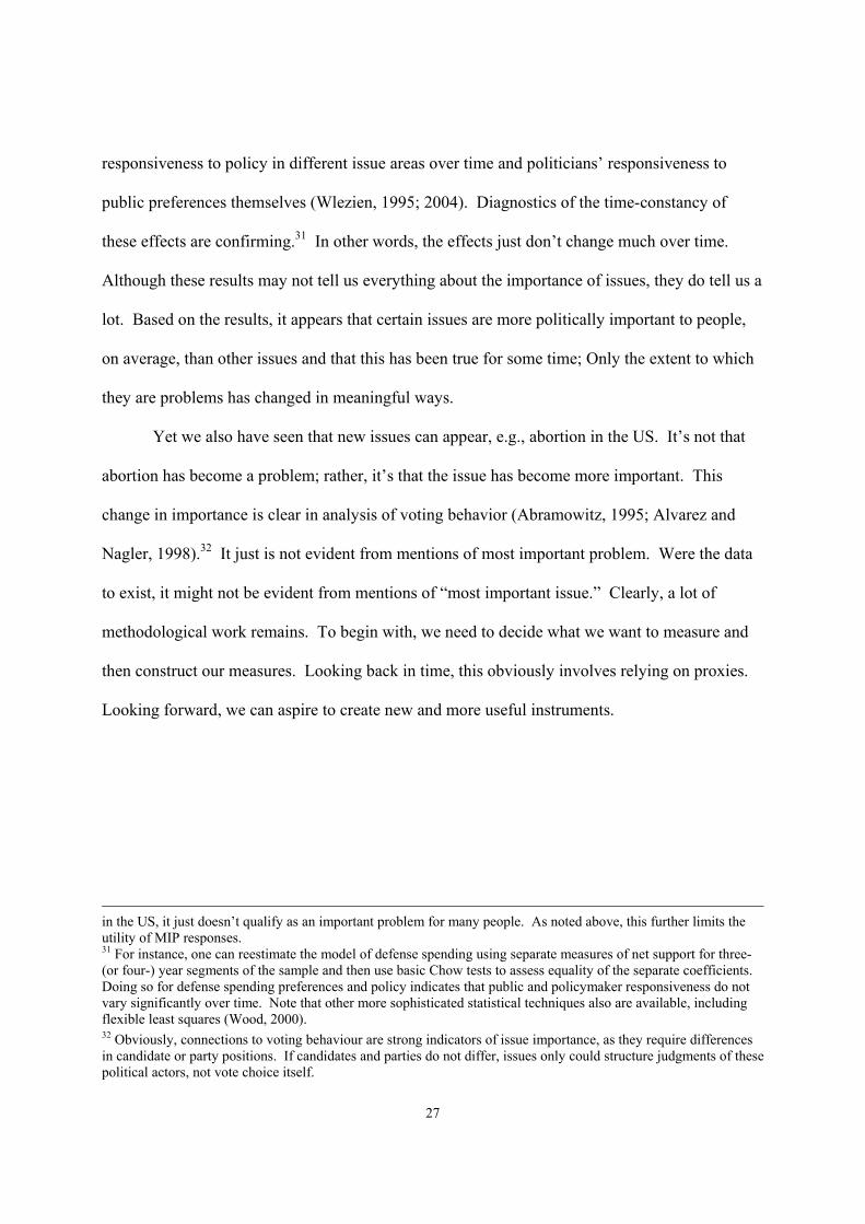
—Figure 1 about here—

Figure 1 plots the basic data. It shows the percentages of respondents offering MIP

11 Data are missing in four years during the period—1949, 1953, 1955, and 1959—but this does not impact any of our statistical analyses, which focus on the period since 1973. 12 This is of some consequence, particularly if one conceives of MIP responses as issue salience weights. That is, the sum of the weights will exceed 1.0 for some individuals and the public as a whole. Of course, this makes little sense, just as one really can’t give 110 percent. 13 That is, MIP in a particular category Y equals 100*YMIPt / TMIPt, where the superscript T designates “Total.” Even assuming that YMIPt is constant, when TMIPt increases (decreases) the percentage owing to YMIPt will decrease

10

responses in the three general categories—foreign affairs, the economy, and other—between

1945 and 2000. We can see that MIP responses within the categories vary a lot over time, but it

is hard to see much else. In Figure 2, which plots only foreign and economic responses, we can

detect more pattern. The foreign policy mentions are large in number early in the series and

comparatively low later on. Economic mentions, conversely, are low early on and then increase

sharply through the 1970’s and into the 1980’s, before dropping off sharply, bouncing up in the

early 1990’s, and then continuing to fall through the end of the series. There thus is some

suggestion of a trade-off between economic and foreign mentions.

—Figure 2 about here—

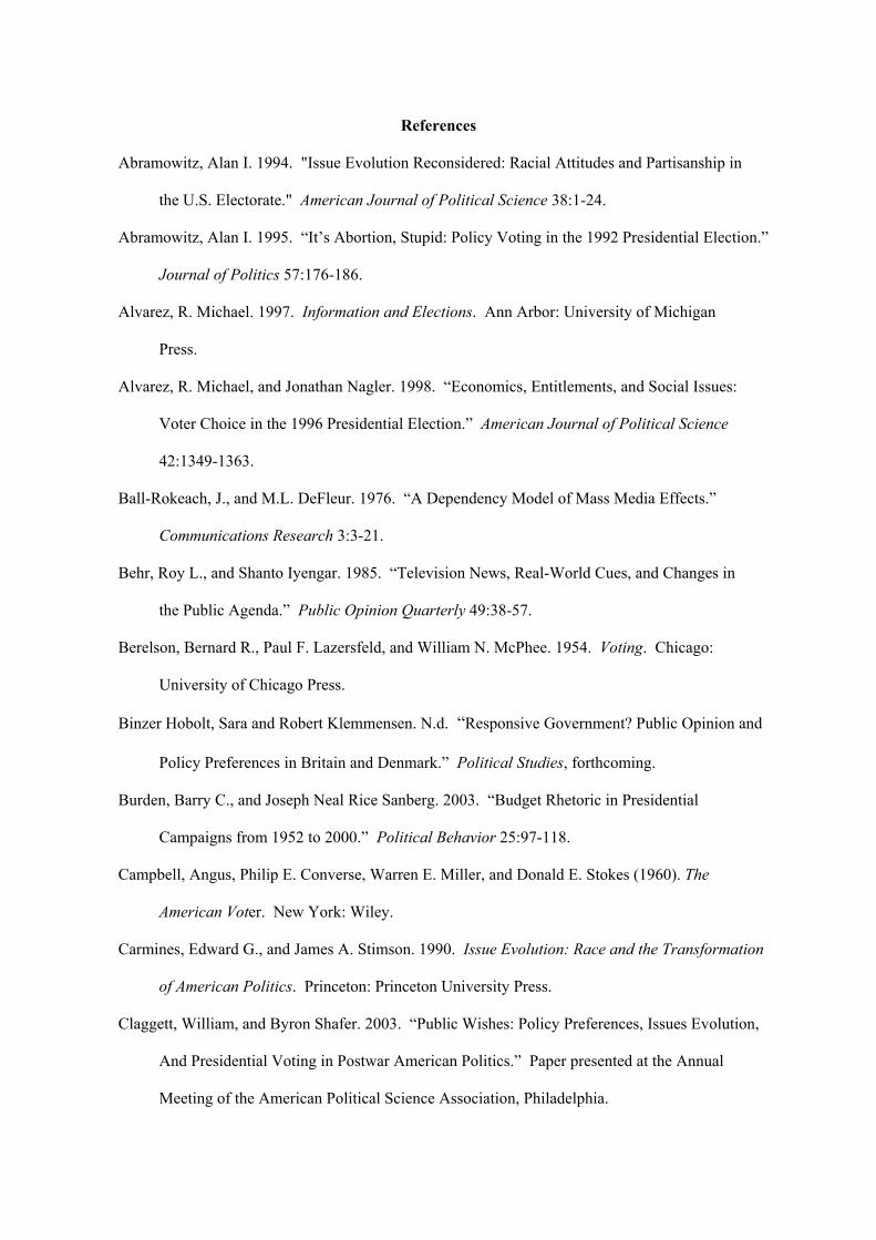
Figure 3 displays the sum of economic and foreign mentions alongside the mentions of

other—non-economic, non-foreign responses. In the figure we can see that mentions of “other”

problems are low early on, jump abruptly during the 1960’s and then decline fairly consistently

through the early 1980’s, when the numbers rebound. They explode through the late 1990’s.

There also is evidence of interdependence between the combined economic-foreign responses on

the one hand and other MIP responses on the other, as increases in the one tend to correspond

with decreases in the other. Indeed, the two series are virtual mirror images of each other over

time.

—Figure 3 about here—

Now, let us explicitly address how much of the variation in MIP responses is due to

changes in importance on the one hand and changes in problem status on the other. We can’t

easily identify the former, but we can explore the latter. That is, we can measure the variation in

“problem” status over time and assess its covariation with MIP responses. In theory, this would

tell us quite a lot about the variation in importance. It is not a perfect strategy, however, as it

(increase) by definition.

11

may be that problem and importance are positively correlated over time, i.e., that when

something becomes a problem it also becomes important. It is a useful—and necessary—first

step, however. We also can take further steps, as we will see. For the analysis, let us focus only

on economic and foreign problems, where reasonable instruments can be found. The literature

offers little basis for tapping the variation in “other” problems, at least in any very general way

across the many different domains (see Soroka, 2002).

There are various indicators of problems with the economy. This analysis relies on

leading economic indicators (LEI) from the Commerce Department, distributed by The

Conference Board. The measure used in the analysis represents the mean annual value of LEI.

The measure includes both objective indicators and the important subjective indicator— the

Index of Consumer Expectations from the University of Michigan.14 It offers useful information

about both the level and direction of the US economy (see, e.g., Wlezien and Erikson, 1996). It

also outperforms measures of coincident and lagging indicators in predicting economic MIP

mentions. (See Appendix A.) For expository purposes, the variable is inverted, so high values

indicate a bad economy and low values a good one. Thus, the measure should be positively

related to economic MIP mentions over time.

There are fewer indicators of problems with foreign policy, either objective or subjective.

We nevertheless do have some indication of public perceptions of the Soviet Union, the primary

reliable source of threat to the US during the period. Specifically, we have a measure of public

dislike of Russia from responses to the like/dislike item in the GSS and surveys conducted by the

Gallup Organization. These responses appear to capture a good portion of the variation in

14 The nine objective indicators are: average weekly hours worked in manufacturing, average weekly claims for unemployment insurance, manufacturers’ new orders for consumer goods and materials, manufacturers’ new orders for nondefense capital goods, building permits for new private housing, Standard and Poor’s 500 stock prices, the money supply (M2), the interest rate spread between 10-year Treasury bonds and federal funds, and vendor

12

perceived national security threat over time, in effect, the degree to which foreign affairs were a

problem in the eyes of the public.15 They do not capture all of the variation in national security

over time, of course, and thus permit only a very conservative test. The specific measure

represents the percentage of people that dislikes Russia minus the percentage that likes the nation

(see Wlezien, 1995; 1996). Unfortunately, the data are available only since 1973, which clearly

limits the time frame for our analysis. Note also that the question was asked only in alternate

years after 1992, and the value from that year is simply carried forward in the ensuing years.16

The variable should be positively related to foreign policy MIP mentions over time: When net

public of dislike increases, mentions of foreign policy MIP are expected to increase.

—Table 1 about here—

Let us now turn to an analysis of economic and foreign policy MIP responses. Table 1

contains the results of regressing economic and foreign mentions on the respective indicators of

economic and foreign problems. The lagged level of MIP responses also is included in each

model. The results confirm our expectations. That is, MIP responses are predicted by the degree

to which there are problems within categories. The positive significant coefficient for (inverted)

leading economic indicators in the first column indicates that when the economy weakens,

economic mentions increase. In the second column we can see that the same is true for national

security and foreign policy responses—when net dislike of Russia increases, foreign mentions

increase. It thus would appear that the degree to which the economy and national security are

performance (slower deliveries diffusion index). For more information on the construction of the index, see the Conference Board website: http://www.globalindicators.org/. 15 That is, they follow standard interpretations of U.S.-Soviet relations over time, marking low relative dislike in the mid-1970's and then tending to erode before reaching a peak of dislike in 1980. The measure levels off during the mid-1980's and drops sharply thereafter. While imperfect, in that it does not incorporate information about national security in general, the measure evidently does capture much of the apparent threat from the Soviet Union over the period. 16 The question was not included in the 1993 GSS and there was no GSS in 1995, 1997, and 1999. Although carrying forward the 1992 value may be a less than perfect solution, notice that the coding that results is consistent with the clearly reduced importance of Russian relations to US national security. Linear interpolation makes little

13

problems structures the variation in MIP responses within those areas. This makes perfect sense

and is exactly as one would expect given the previous literature (Ball-Rokeach and DeFleur,

1976; MacKuen and Coombs, 1981, Soroka, 2002).

Let us now see whether the variation in problem status in one category affects MIP

responses in the other categories. To do this, we simply include the measures of both leading

economic indicators and net dislike into each of the models. We also estimate a parallel model

of “other” MIP responses. We are interested in seeing whether the coefficients of the variables

are negatively-signed and statistically significant. This would indicate that when the causes of

MIP mentions in one category go up, the MIP mentions for the other categories go down. The

results are shown in Table 2.

—Table 2 about here—

It is clear in the table that the degree to which one category is a problem influences

mentions of other categories. In the first column, we can see that when economic security

worsens, the percentage of respondents naming foreign problems decreases. The coefficient not

only is negative; it is highly reliable. Interestingly, the effect holds only for “defense/military”

mentions and not those of a more general “international” flavor. This can be seen in Table 3,

which contains the results of estimating the model separately for the two categories.17 Back in

Table 2, we can see in the third column that mentions of other—non-economic, non-foreign—

problems shift in the same way. When economic security weakens, and economic mentions

increase, the “other” MIP mentions decline. Notice also that the sum (-1.47) of the estimated

effects of leading economic indicators on foreign and other problems is virtually equal and

opposite to its effect (1.37) on economic mentions. Changes in economic security thus leave

difference. 17 Purely “international” problems are entirely unrelated to variation in our indicators of either national or economic security. Presumably, variation in these problems evidently is largely exogenous to the system.

14

total MIP responses essentially unchanged.

In Table 2 we also can see that changes in national security have similar effects on

economic and other problems, though these effects are not highly reliable when the categories

are taken separately. While the coefficients for net dislike in the first and third columns are

appropriately negative, they are not even close to conventional levels of statistical significance.

When economic and other MIP mentions are taken together, however, the net effect of shifting

national security is much more reliable (p < .05, one-tailed). The estimated effect on these

combined responses is -.17, slightly less in absolute terms than its effect (.19) on foreign affairs

responses in Table 2. As we saw for the economic security, the effects of changing national

security on MIP mentions within the domain come at the expense of—not in addition to—

mentions in other domains.

—Table 3 about here—

The foregoing analysis is important. It implies that much of the movement in MIP

responses not only is unrelated to changes in importance per se; much is unrelated to changes in

the degree to which the particular domain is a problem. A large part of the variance in MIP

responses within domains reflects the degree to which there are problems in other domains. It

ultimately appears that much of the variance in MIP responses is unrelated to variation in

importance.

But, what portion of the variance is due to changes in importance? It is fair—indeed,

appropriate—to wonder. The problem is that we can’t tell for sure. However, based on the

foregoing models, we can estimate the amount in each category that is due to variance in

problem status, both within and without each category. In one sense, the remaining, residual

variance from our analysis constitutes an upper-bound estimate of the variance that is due to

changing importance. Indeed, the estimate seems a quite liberal one because it contains basic

15

sampling (and other survey) error as well as unmeasured variation in problem status. The

estimate actually could be a conservative one, as it may be that the variance attributed to changes

in problem status partly capture changes in importance, noted earlier. These possibilities can be

to some extent addressed in the analyses of defense spending opinion and policy that follow.

Estimating the proportion of variance that is unrelated to our indicators of problem variation

provides directly relevant information. To generate the numbers, it is necessary to first

reestimate the equations in Table 2 (and Table 3) excluding the lagged dependent variables,

which may contain information unrelated to problem status.18 The results of the analysis of

variance are shown in Table 4.

—Table 4 about here—

In the table it is clear that most of the variance in MIP responses reflects changes in our

basic indicators of problem status. The first column shows the variance of MIP responses in the

different categories—economic, foreign, and other. The second column reports the variance

explained by the basic indicators of economic and national security used above. The third

column shows the residual variance and the final column the percentage of the total variance that

is residual. The two indicators account for just over 77 percent of the variance in economic MIP

responses and about 55 percent of foreign affairs mentions (58 percent for “defense”).

Approximately 68 percent of the variance in non-economic, non-foreign MIP is predicted by the

indicators of economic and national security. This puts in perspective—and makes more

understandable—the stunning rise in “other” MIP, e.g., education and drugs and crime, through

the 1990’s (and the subsequent drop in 2001 and 2002).19 Of course, nontrivial portions of

variance remain in each of the three broad categories. They may be the simple result of survey

18 Including lags of the problem status indicators makes no significant difference to the analyses. All of these results are available on request. 19 That is, as peace and prosperity broke out through the 1990’s, people had to look elsewhere for their most

16

error. They may reflect unmeasured variation in problem status, either real or perceived. The

possibility remains that the residual variance in MIP responses actually is due to changing

importance of the domains. We can begin to explore these possibilities.

MIP Responses and Importance?

The foregoing analyses reveal potential problems with using aggregate MIP responses as

indicators of the importance of issues or even important problems. Most of the variance reflects

changes in problem status within domains and in other domains. Still, it is important to not

overdraw the conclusion—at least not yet—for at least two reasons that have already been noted.

First, there is surplus variance, and it may be that this to some extent reflects change in issue

importance. Second, it may be that some of the variance we have attributed to changes in

problem status reflects changes in importance, i.e., that problem and importance are positively

correlated over time. Let us consider these possibilities, loosely following Jones’ (1994) logic.

That is, let us consider whether changes in MIP mentions structure opinion-policy dynamics:

both policymaker responsiveness to public preferences and public responsiveness to policy itself.

As Jones has argued, policymakers may be more likely to notice and pay attention to public

opinion for policy in a particular area when the public views that issue as important.20 Likewise,

following Franklin and Wlezien (1997), the public may be more responsive to policy change as

importance increases. If MIP responses capture variation in importance, therefore, we should

expect that policymakers will be more responsive to public opinion and/or that the public will be

more responsive to policy behavior itself when MIP is high. It is useful to be more specific

about these expectations, using the thermostatic model of opinion and policy.

important problems. After 9/11 and the recession that followed, they didn’t. 20 This reflects the now classic perspective. See, e.g., McCrone and Kuklinski, 1979; Geer, 1996; Hill and Hurley, 1998.

17

A Model of Opinion-Policy Dynamics, Including MIP

The thermostatic model (Wlezien, 1995; 1996) implies that policymakers respond to

public preferences for policy change and that the public, in turn, adjusts its preferences in

response to what policymakers do. To begin with, the public’s preference for ‘more’ or ‘less’

policy—its relative preference, R—represents the difference between the public’s preferred level

of policy (P*) and the level it actually gets (P).

(3) Rt = P*t - Pt

Rt = Rt-1 + ∆P*t - ∆Pt

∆Rt = ∆P*t - ∆Pt.

Thus, as the preferred level of policy or policy itself changes, the relative preference signal

changes accordingly. Changes in the preferred level obviously have positive effects. Changes in

policy have negative ones: When policy increases (decreases), the preference for more policy

decreases (increases). This negative feedback is the real crux of the thermostatic model. The

public is expected to respond currently to actual policy change when put into effect. This is

straightforward, at least in theory. It is less straightforward in practice.

Most importantly, we typically do not directly observe P* over time. With some

exceptions, survey organizations do not ask people how much policy they want. Instead, these

organizations usually ask about relative preferences, e.g., whether we are spending "too little,"

whether spending should "be increased," or whether we should "do more.” The public

preference, however defined, also is necessarily relative. In one sense, this is quite convenient,

as we can measure the thermostatic signal the public sends to policymakers. Because we must

rely on instruments to estimate P*—and because metrics of the other variables differ—it is

necessary to rewrite equation 3 from above as follows:

18

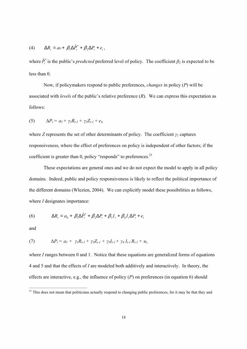
(4) tttt ePPaR +∆+∆+=∆ 2*

1 0 ˆ ββ ,

where *t̂P is the public’s predicted preferred level of policy. The coefficient β2 is expected to be

less than 0.

Now, if policymakers respond to public preferences, changes in policy (P) will be

associated with levels of the public’s relative preference (R). We can express this expectation as

follows:

(5) ∆Pt = a1 + γ1Rt-1 + γ2Zt-1 + et,

where Z represents the set of other determinants of policy. The coefficient γ1 captures

responsiveness, where the effect of preferences on policy is independent of other factors; if the

coefficient is greater than 0, policy “responds” to preferences.21

These expectations are general ones and we do not expect the model to apply in all policy

domains. Indeed, public and policy responsiveness is likely to reflect the political importance of

the different domains (Wlezien, 2004). We can explicitly model these possibilities as follows,

where I designates importance:

(6) ttttttt ePIIPPaR +∆++∆+∆+=∆ 432*

1 0ˆ ββββ

and

(7) ∆Pt = a1 + γ1Rt-1 + γ2Zt-1 + γ3It-1 + γ4 It-1 Rt-1 + ut,

where I ranges between 0 and 1. Notice that these equations are generalized forms of equations

4 and 5 and that the effects of I are modeled both additively and interactively. In theory, the

effects are interactive, e.g., the influence of policy (P) on preferences (in equation 6) should

21 This does not mean that politicians actually respond to changing public preferences, for it may be that they and

19

depend on the level of I. Thus, we are most interested in whether the interactive variables in

equations 6 and 7 have significant effects. That is, we want to know whether the B4 is less than 0

and γ4 is greater than 0, which would tell us that the level of I influences either public or

policymaker responsiveness. In the extreme, responsiveness would depend entirely on I and B2

and γ1 would equal 0.

Of course, we do not have a direct measure of I, and we want to see whether the measure

MIP contains relevant information, as many scholars suppose. This is straightforward. We can

use MIP as our measure of I in equations 6 and 7 and assess the parameters B4 and γ4. As we

already have seen, however, MIP responses capture variation in problem status. It may be that

this variation is highly correlated with importance over time, in which case simply using MIP

would be appropriate. Alternatively, it may be that this variation is largely uncorrelated with

changes in importance over time, in which case using MIP would not be right. A more

appropriate specification then would be to include only the variation in MIP that is due to

variation in importance per se. Consider MIP* to be the variation in MIP purged of the variation

due to changing problem status, both within the particular domain and other domains, from Table

4. To see whether it matters, we simply substitute MIP* for I in equations 6 and 7. We can see

what happens when we do.

An Expository Empirical Analysis

For this analysis, consider the interrelationships between public preferences and policy

change in a single domain—spending on defense in the U.S. The decision reflects a variety of

considerations. First, and most importantly, we know a good amount about defense MIP from

the foregoing analysis. This is of obvious significance given the theoretical model outlined

the public both respond to something else. All we can say for sure is that the coefficient (γ1) captures policy

20

above. Second, we have good data on defense spending decisions and public spending

preferences themselves over a reasonable time period, 1973-1994. Third, the thermostatic model

appears to work quite well in the domain. That is, there is strong evidence of public

responsiveness to policy and policymaker responsiveness to preferences (Wlezien, 1996).22 It

thus makes sense to ask: Does the evident opinion representation and policy feedback vary with

MIP? Let us begin with the public itself.

An Analysis of Public Responsiveness to Policy

The basic model of public preferences follows Wlezien’s (1996) research. The

dependent variable is the difference in net support for spending, where net support is the

percentage of people who think we are spending “too little” minus the percentage of people who

think we are spending "too much.” Thus, as noted above, the measure taps relative preferences.

The data are based on responses to the standard question: Are we spending too much, too little,

or about the right amount on the military, armaments, and defense? The General Social Survey

(GSS) has asked this item in every year between 1973 and 1994, with the exception of 1979,

1981, and 1992. Fortunately, Gallup asked the same question in those years. Since 1994, data

are available only in alternate years, which clearly limits our analysis. From these data, we

nevertheless can construct annual time series of public preferences for spending that cover 1973-

1994.

Recall that the thermostatic model implies that the public’s relative preference for

spending represents the difference between the public’s preferred level of spending and spending

itself. It is easy to measure spending, which we can draw from the Budget of the United States

Government. This analysis relies on appropriations data instead of actual spending, the latter of

responsiveness in a statistical sense, that is, the extent to which public preferences directly influence policy change, other things being equal.

21

which often lag far behind actual budgetary decisions, and the numbers are adjusted for

inflation.23 Following equation 4, a first difference measure is used. Now, as noted above, we

do not have a measure of the public’s preferred level of spending, so it is necessary to rely on

instruments. For this analysis, the measure of net dislike of Russia is used. We already have

seen that it nicely captures variation in problem status over time. It also has been shown to

powerfully predict variation in preferences for defense spending in the US (Wlezien, 1995;

1996).

The results of estimating this basic model are shown in the first column of Table 5.24

Here we can see that changes in net support are positively related to changes in Net Dislike:

When dislike of Russia increases, support for more spending increases. We also can see that

changes in net support are negatively related to changes in appropriations: When appropriations

increase, support for more spending decreases. These patterns are already known. The results

serve as the baseline for our analysis including MIP.

—Tables 5 about here—

Now, let’s see whether the MIP responses add any additional information. To begin

with, let us estimate equation 6 using raw defense mentions. The results of this analysis are

shown in the second column of Table 5. Notice first that the coefficient for the additive MIP

variable actually is positive, though too unreliable to credit. More importantly, the coefficient

for the interactive variable is “0.” The performance of this model is lower, as can be seen from

the adjusted R-squared, which goes down, and the mean squared error, which goes up. Thus, we

22 For comparative perspectives, see Eichenberg and Stoll (2003) and Soroka and Wlezien (2004). 23 For a comparative analysis of appropriations and outlays, see Wlezien and Soroka (2003). Real dollar values are calculated by dividing current dollar values into the gross national product implicit price deflator (1987=1.00), from The National Income and Product Accounts. 24 The model also includes a control for the Iraq-Kuwaiti crisis in 1991-1992.

22

are better off not including MIP in the model. This is an important result: It implies that defense

MIP responses do not capture variation in the importance of defense-related issues.

As noted above, however, there is another perhaps more appropriate way to capture the

information in MIP responses. Our analyses have shown us that the variation in defense MIP

responses to a large extent is due to changes in national and economic security over time. This

variation reflects the degree to which foreign policy (and the economy) is a problem, and it may

be that the variation is unrelated to changes in importance. The remaining variation in MIP

responses may be due to changing importance. It thus may be more appropriate to model the

effects of this “residual” portion of MIP responses instead of the whole. This is fairly easy to do.

That is, we can use the residuals from the analysis summarized in Table 4. To be absolutely

clear, the residuals are from the regression of defense MIP on net dislike and leading economic

indicators.25 The results of substituting this “purged” measure for raw MIP in our analysis of

public preferences are shown in the third column of Table 5.

These results differ somewhat from those using the raw measure of MIP. That is, the

additive effect of MIP* is negative and the interactive effect positive. The latter runs completely

contrary to our expectations, though it is not statistically significant. The results are telling: To

the extent MIP responses capture variation in importance, it seems clear that the importance of

the defense domain remained essentially unchanged during the period, at least in the public’s

mind. Let us now consider whether this also is true for policymakers in their response to public

opinion itself.

An Analysis of Policymaker Responsiveness to Public Preferences

25 The estimated equation is as follows: Defense MIPt = 6.39 + .23 Net Disliket - .57 Leading Economic Indicatorst, R-squared= .61; Adjusted R-squared=.58; Mean squared error=5.08.

23

The model of spending policy also follows Wlezien’s (1996) research. The dependent

variable represents the first difference of real dollar-valued appropriations (in billions of 1987

dollars) for defense. The independent variables include the party of the president, the party

composition of Congress, and a measure of net support for defense spending. Given that the

measure of net support captures relative preferences, changes in appropriations are expected to

be positively related to the levels of net support for spending. Politicians are expected to respond

currently. In the budgetary context, this means that the change in appropriations for fiscal year t

follows the level of net support in year t-1, when the bulk of appropriations for fiscal year t are

made.

As noted above, measures of the party of the president and the party composition of

Congress also are included in the models. The former variable takes the value “1” under

Democratic presidents and “0” under Republican presidents, and the latter variable represents the

average percentage of Democrats in the House and Senate. Like for net support, these political

variables are measured during year t-1. Thus, the analysis that follows relies on a very simple

model that includes the party of the president, the party composition of Congress, and the

measure of public preferences for spending.26

The results from estimating the original model are shown in the first column of Table 6.

Here we see that changes in appropriations do closely follow public preferences for defense

spending over time. As indicated by the positive, significant coefficient for net support, when

public support for more defense spending is high, politicians tend to provide more defense

appropriations. Defense appropriations also reflect the party affiliation of the president. Based

on the coefficient in Table 6, the change in defense appropriations is about 11 billion (1987)

26 The model also includes a control for the Iraq-Kuwaiti crisis in 1992

24

dollars higher under Republican presidents than under Democratic presidents, given public

preferences. The Congressional composition has no effect, however.

— Table 6 about here —

Now, let us see what MIP responses add. To begin with, let us estimate equation 7 using

the raw measure of defense MIP, the results of which are shown in the second column of Table

6. Here we can see that the coefficient for the important interactive variable is appropriately

positive but does not approach conventional levels of statistical significance. Adding the MIP

variables, moreover, actually reduces model performance. As we saw with public

responsiveness, it appears that raw MIP responses offer little additional information to our

understanding of policy, that is, above and beyond what is reflected in public policy preferences.

Analysis using the purged MIP variable (MIP*) is more promising, as can be seen in the third

column of Table 6. Here, the coefficient for the interactive variable not only is positive; it

borders on statistical significance (p = .08, one-tailed).27

The last result is suggestive about the effect of importance. Notice first that the result

implies that importance and problem status are not highly correlated over time. That is, the

“purged” MIP* measure outperforms the raw MIP measure. The fact that the interactive

coefficient borders on statistical significance even implies that MIP responses may capture

something meaningful about the public importance of issues, at least as perceived by

policymakers. (We should not forget, after all, that MIP responses had absolutely no effect on

the public’s responsiveness to policy change.) As we more fully control for the variation in

problem status, we may see more clearly the variation in importance. This remains to be seen,

27 Taking into account sampling error seems to make little difference. First, the sampling error variance of defense MIP presumably is very small relative to the true variance. This is difficult to prove, but consider that the mean percentage of respondents stating a defense MIP since 1973 is only 6.1 and the observed yearly variance is 61 percent. Even assuming sample sizes of 100, the estimated reliability would approach 0.90. Second, the error variance is shared between the predicted and residual components, both of which are based on survey responses.

25

however. Even so, the variation nevertheless is small, at least when compared with that due to

changing problem status. Recall from Table 4 that our very basic measures of defense and

economic problem status already account for approximately 60 percent of the variance in defense

MIP; A more complete accounting would only increase the percentage. It thus appears that

importance is at best a comparatively small part of the variance of defense MIP over time.

Although MIP responses have fluctuated dramatically over time, the importance of the defense

domain has nevertheless remained largely unchanged. This may be true for other issues as well.

Concluding Thoughts

One might think that an important issue is salient by definition. This is not the case given

traditional measurement, which relies on responses to questions about the “most important

problem” facing the nation. Whether an issue is an “important problem” to the public is a

function of importance and the degree to which it is a problem. The most important problem, in

turn, is just that, the plurality important problem winner. At best, then importance and measured

salience are two related, but different things. At worst, problems and issues are two

fundamentally different things, one about conditions and the other about policy. The foregoing

analyses indicate that most important problem responses are largely driven by problem status;

indeed, a large part of the variation in particular categories reflects the degree to which other

things are problems. These responses simply tell us little, if anything, about the importance of

issues. This is not surprising; it actually may seem obvious. Scholars nevertheless continue to

use these responses to indicate importance. This practice is mistaken. It may be that MIP

responses nicely indicate “prominence” or other aspects of salience. The problem is that we just

don’t know. In effect, we are doing science backwards, making do with existing instruments

Even assuming a reliability of 0.90, however, the results change only marginally (b = 0.10, s.e. = 0.06).

26

without knowing or being clear about what they represent.

This is not to say that the importance of issues does not change over time. But, how

should one go about measuring this changing importance? It is not straightforward capturing

current changes let alone those that have passed us by. As for the future, one possibility is to

simply ask people about the importance of different issues. This has been and is being tried

(Fournier, et al, 2003) and, while some progress is being made, the answer still remains elusive.28

To begin with, as noted earlier, it is not clear exactly how respondents interpret questions asking

about the importance of a particular issue. Do they interpret it to mean the general importance to

society? The general importance to themselves? The importance to their vote choice? There are

other possibilities. If we are interested in political relevance, however, perhaps we should ask

about the “importance” of an issue to their vote choice. This is becoming quite common, but it’s

not clear what the responses reveal. What we do know is that most people think most issues are

“extremely” important or “very” important.29

We don’t have to ask people, however. We can observe their behavior. This is of

obvious relevance when trying to characterize the past, that is, where new innovations in

question wording are of no use. Studies of voting behavior and election outcomes have taught us

quite a lot, both at particular points in time and over time (Asher, 1992; Abramowitz, 1994;

Claggett and Shafer, 2003; also see Stokes, 1966). We know that certain issues have mattered

quite consistently over time, such as the economy. Other issues also have mattered, such as

national security and social welfare in the US.30 Similar patterns are evident in the public’s

28 See Janowitz’s (2002) interesting analysis. 29 Consider the following results from a Newsweek Poll conducted February 19-20, 2004. Respondents were asked to tell whether a series of issues were “very important, somewhat important, not too important, or not at all important” in determining their vote for president in that year. The percentages saying “very important” are as follows: economy (77), education (72), health care (70), terrorism (69), American jobs (68), the situation in Iraq (63), taxes (55). Source: www.pollingreport.com/prioriti.htm. 30 Note that MIP mentions of welfare are very rare. Although the issue clearly is important to voting and elections

27

responsiveness to policy in different issue areas over time and politicians’ responsiveness to

public preferences themselves (Wlezien, 1995; 2004). Diagnostics of the time-constancy of

these effects are confirming.31 In other words, the effects just don’t change much over time.

Although these results may not tell us everything about the importance of issues, they do tell us a

lot. Based on the results, it appears that certain issues are more politically important to people,

on average, than other issues and that this has been true for some time; Only the extent to which

they are problems has changed in meaningful ways.

Yet we also have seen that new issues can appear, e.g., abortion in the US. It’s not that

abortion has become a problem; rather, it’s that the issue has become more important. This

change in importance is clear in analysis of voting behavior (Abramowitz, 1995; Alvarez and

Nagler, 1998).32 It just is not evident from mentions of most important problem. Were the data

to exist, it might not be evident from mentions of “most important issue.” Clearly, a lot of

methodological work remains. To begin with, we need to decide what we want to measure and

then construct our measures. Looking back in time, this obviously involves relying on proxies.

Looking forward, we can aspire to create new and more useful instruments.

in the US, it just doesn’t qualify as an important problem for many people. As noted above, this further limits the utility of MIP responses. 31 For instance, one can reestimate the model of defense spending using separate measures of net support for three- (or four-) year segments of the sample and then use basic Chow tests to assess equality of the separate coefficients. Doing so for defense spending preferences and policy indicates that public and policymaker responsiveness do not vary significantly over time. Note that other more sophisticated statistical techniques also are available, including flexible least squares (Wood, 2000). 32 Obviously, connections to voting behaviour are strong indicators of issue importance, as they require differences in candidate or party positions. If candidates and parties do not differ, issues only could structure judgments of these political actors, not vote choice itself.

28

Appendix A: How the Economy Matters

Table A1. A Diagnosis of Economic Effects, 1973-2000 ------------------------------------------------------------------------------------ Independent Variable Economic MIP Responses ------------------------------------------------------------------------------------ Intercepta 19.83* 31.69** 35.00** (11.41) (8.26) (1.10) MIPt-1 0.68** 0.50** 0.47** (0.17) (0.13) (0.11) Lagging Economic 1.19 --- --- Indicatorst (inverted) (.98) Coincident Economic --- .61** -.61 Indicatorst (inverted) (.17) (0.41) Leading Economic --- --- 2.25** Indicatorst (inverted) (0.70) R-squared .67 .77 .84 Adjusted R-squared .65 .75 .82 Standard Error 12.85 10.70 9.11 Durbin-Watson 1.62 1.72 1.85 N = 28, ** p < .01 * p < .05 (two-tailed) ----------------------------------------------------------------------------------- Note: The numbers in parentheses are standard errors.

References

Abramowitz, Alan I. 1994. "Issue Evolution Reconsidered: Racial Attitudes and Partisanship in

the U.S. Electorate." American Journal of Political Science 38:1-24.

Abramowitz, Alan I. 1995. “It’s Abortion, Stupid: Policy Voting in the 1992 Presidential Election.”

Journal of Politics 57:176-186.

Alvarez, R. Michael. 1997. Information and Elections. Ann Arbor: University of Michigan

Press.

Alvarez, R. Michael, and Jonathan Nagler. 1998. “Economics, Entitlements, and Social Issues:

Voter Choice in the 1996 Presidential Election.” American Journal of Political Science

42:1349-1363.

Ball-Rokeach, J., and M.L. DeFleur. 1976. “A Dependency Model of Mass Media Effects.”

Communications Research 3:3-21.

Behr, Roy L., and Shanto Iyengar. 1985. “Television News, Real-World Cues, and Changes in

the Public Agenda.” Public Opinion Quarterly 49:38-57.

Berelson, Bernard R., Paul F. Lazersfeld, and William N. McPhee. 1954. Voting. Chicago:

University of Chicago Press.

Binzer Hobolt, Sara and Robert Klemmensen. N.d. “Responsive Government? Public Opinion and

Policy Preferences in Britain and Denmark.” Political Studies, forthcoming.

Burden, Barry C., and Joseph Neal Rice Sanberg. 2003. “Budget Rhetoric in Presidential

Campaigns from 1952 to 2000.” Political Behavior 25:97-118.

Campbell, Angus, Philip E. Converse, Warren E. Miller, and Donald E. Stokes (1960). The

American Voter. New York: Wiley.

Carmines, Edward G., and James A. Stimson. 1990. Issue Evolution: Race and the Transformation

of American Politics. Princeton: Princeton University Press.

Claggett, William, and Byron Shafer. 2003. “Public Wishes: Policy Preferences, Issues Evolution,

And Presidential Voting in Postwar American Politics.” Paper presented at the Annual

Meeting of the American Political Science Association, Philadelphia.

Clarke Harold, Nitish Dutt, and Jonathon Rapkin. 1997. “Conversations in Context.” Political

Behavior 19:19-39.

Converse, Philip E. 1975. "Public Opinion and Voting Behavior." In Fred I. Greenstein and

Nelson W. Polsby, (eds.), Handbook of Social Science, Volume 4. Reading, Mass.:

Addison-Wesley.

-----. 1964. "The Nature of Belief Systems in Mass Publics." In David Apter, ed., Ideology and

Discontent. New York: Free Press.

Deutsch, Karl W. 1963. The Nerves of Government. New York: Free Press.

Downs, Anthony. 1957. An Economic Theory of Democracy. New York: Harper.

Durr, Robert H. 1993. "What Moves Policy Sentiment?" American Political Science Review

87:158-170.

Easton, David. 1965. A Framework for Political Analysis. Englewood Cliffs, N.J.: Prentice-

Hall.

Eichenberg, Richard, and Richard Stoll. 2003. “Representing Defense: Democratic Control of the

Defense Budget in the United States and Western Europe.” Journal of Conflict Resolution

47:399-423.

van der Eijk, Cees and Mark N. Franklin. 1996. Choosing Europe? The European Electorate

and National Politics in the Face of Union. Ann Arbor, MI: University of Michigan Press.

Epstein, Lee and Jeffrey A. Segal. 2000. “Measuring Issue Salience.” American Journal of

Political Science 44:66-83.

Erikson, Robert S., Gerald C. Wright, and John P. McIver. 1993. Statehouse Democracy:

Public Opinion and Policy in the American States. New York: Cambridge University

Press.

Erikson, Robert S. and David Romero. 1990. “Candidate Equilibrium and the Behavioral

Model of the Vote. American Political Science Review 84:1103-1126.

Feeley, T. Jens, Bryan D. Jones, Heather Larsen. 2001. Public Agendas: Most Important

Problem Polling Data, 1939-2001. Seattle, WA: University of Washington (Portions

of this data originally compiled by the Gallup Organization) [Computer file].

Ferejohn, John A. and James H. Kuklinski (eds.). 1990. Information and Democratic Processes.

Urbana: University of Illinois Press.

Fournier, Patrick, Andre Blais, Richard Nadeau, Elisabeth Gidengil, and Neil Nevitte. 2003.

“Issue Importance and Performance Voting.” Political Behavior 25: 51-67.

Franklin, Mark and Christopher Wlezien. 1997. "The Responsive Public: Issue Salience, Policy

Change, and Preferences for European Unification." Journal of Theoretical Politics 9:

247-263.

Geer, John G. 1996. From Tea Leaves to Opinion Polls. New York: Columbia University Press.

Glasgow, Garrett. 1998. “Comparing Measures of Issue Salience in a Spatial Model of Voting.”

Unpublished manuscript, California Institute of Technology.

Hartley, Thomas and Bruce Russett. 1992. "Public Opinion and the Common Defense: Who

Governs Military Spending in the United States?" American Political Science Review

86:905-915.

Hill, Kim Quaile, and Patricia A. Hurley. 1998. “Dyadic Representation Reappraised.”

American Journal of Political Science 43: 109-137.

Jackson, John. 1975. “Issues, Party Choices, and Presidential Voting.” American Journal

Of Political Science 19:161-186.

Jacoby, William G. 1994. "Public Attitudes Toward Government Spending." American

Journal of Political Science 38: 336-361.

Janowitz, Paul. 2002. “Issue Salience: A Fresh Look with a New Measure.” Paper presented

at the Annual Meeting of the Midwest Political Science Association, Chicago.

Jones, Bryan D. 1994. Reconceiving Decision-Making in Democratic Politics: Attention,

Choice, and Public Policy. Chicago: University of Chicago Press.

Jones, Bryan D., Frank Baumgartner and James L. True. 1998. “Policy Punctuations: U.S.

Budget Authority, 1947-1995.” Journal of Politics. 60:1-33.

Krosnick, Jon A. 1988. “The Role of Attitude Importance in Social Evaluation: A Study of

Policy Preferences, Presidential Candidate Evaluation, and Voting Behavior.” Journal

of Personality and Social Psychology 55:196-210.

MacKuen, Michael B., and Steven L. Coombs. 1981. More Than News: Media Power in

Public Affairs. Beverly Hills, CA: Sage Publications.

McCombs, Maxwell. 1999. “Personal Involvement with Issues on the Public Agenda.”

International Journal of Public Opinion Research 11:152-168.

McCombs, Maxwell E., and Donald L. Shaw. 1972. “The Agenda-Setting Function of the

Mass Media.” Public Opinion Quarterly 36:176-185.

McCombs, Maxwell, and Jian-Hua Zhu. 1995. “Capacity, Diversity, and Volatility of the

Public Agenda: Trends from 1954 to 1994.” Public Opinion Quarterly 59:495-525.

McCrone, Donald J. and James H. Kuklinski. 1979. “The Delegate Theory of

Representation.”American Journal of Political Science 23:278-300.

McDonald, Michael D., Ian Budge, and Paul Pennings. 2004. “Choice versus Sensitivity:

Party Reactions to Public Concerns.” European Journal of Political Research 43:

845-868.

Miller, Arthur H., Warren E. Miller, Alden S. Raine, and Thad A. Browne. 1976. "A

Majority Party in Disarray: Policy Polarization in the 1972 Election." American

Political ScienceReview 70:753-778.

Miller, Warren E. and Donald E. Stokes. 1963. "Constituency Influence in Congress,"

American Political Science Review 57:45-56.

Niemi, Richard G., and Larry M. Bartels. 1985. “New Measures of Issue Salience: An

Evaluation.” Journal of Politics 47:1212-1220.

Niemi, Richard G., John Mueller, and Tom Smith. 1989. Trends in Public Opinion: A

Compendium of Survey Data. Westport, Conn.: Greenwood Press.

Rabinowitz, George, James Prothro, and William Jacoby. 1982. “Salience as a Factor in the

Impact of Issues on Candidate Evaluation.” Journal of Politics 44:41-64.

RePass, David E. 1971. "Issue Salience and Party Choice." American Political Science

Review 65:389-400.

River, Douglas. 1988. “Heterogeneity in Models of Electoral Choice.” American Political

Science Review 32:737-758.

Schuman, Howard, Jacob Ludwig, and Jon A. Krosnick. 1986. “Perceived Threat of

Nuclear War, Salience, and Open Questions.” Public Opinion Quarterly 50:519-536.

Sharpe, Elaine. 1999. The Sometime Connection: Public Opinion and Social Policy.

Albany,New York: SUNY Press.

Smith, Tom W. 1985. “America’s Most Important Problems, Part 1: National and

International.” Public Opinion Quarterly 49:264-74.

Sniderman, Paul. 1993. "The New Look in Public Opinion Research." In Ada W. Finifter

(ed.),Political Science: The State of the Discipline II. Washington, D.C.: American

Political Science Association.

Soroka, Stuart N. 2002. Agenda-Setting Dynamics in Canada. Vancouver: University of

British Columbia Press.

Soroka, Stuart N. and Christopher Wlezien. 2004. Degrees of Democracy: Public Opinion and

Policy in Comparative Perspective.” Center for Advanced Study in the Social Sciences

Working Paper, #206. Madrid: Juan March Institute.

Stokes, Donald E., 1966. “Some Dynamic Elements of Contests for the Presidency.”

American Political Science Review. 60:19-28.

Taylor, Shelley. E., & Susan T. Fiske. 1978. “Salience, Attention, and Attribution: Top of the Head

Phenomena.” Advances in Experimental Social Psychology 11:249-288.

Wlezien, Christopher. 2004. “Patterns of Representation: Dynamics of Public Preferences

and Policy.” Journal of Politics 66:1-24.

-----. 1996. "Dynamics of Representation: The Case of U.S. Spending on Defense."

British Journal of Political Science 26:81-103.

-----. 1995. "The Public as Thermostat: Dynamics of Preferences for Spending." American

Journal of Political Science 39:981-1000.

Wlezien, Christopher and Christopher Carman. 2001. “Ideological Placements and Political

Judgments of Government Institutions.” Public Opinion Quarterly 65:550-561.

Wlezien, Christopher and Robert S. Erikson. 1996. “Temporal Horizons and Presidential

Election Forecasts.” American Politics Quarterly 24: 495-512.

Wlezien, Christopher and Stuart Soroka. 2003. “Measures and Models of Budgetary Policy.

Policy Studies Journal 31: 273-286.

Wood, B.Dan. 2000. “Weak Theories and Parameter Instability: Using Flexible Least

Squares to Take Time-Varying Relationships Seriously.” American Journal of Political

Science 44:603-618.

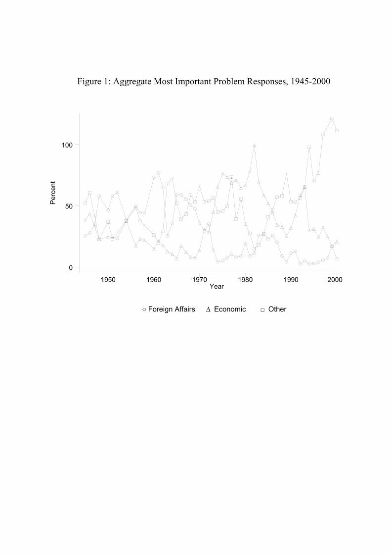
Figure 1: Aggregate Most Important Problem Responses, 1945-2000

Perc

ent

Year1950 1960 1970 1980 1990 2000

0

50

100

○ Foreign Affairs ∆ Economic □ Other

Figure 2: Aggregate Most Important Problem Responses, 1945-2000

Perc

ent

Year1950 1960 1970 1980 1990 2000

0

50

100

○ Foreign Affairs ∆ Economic

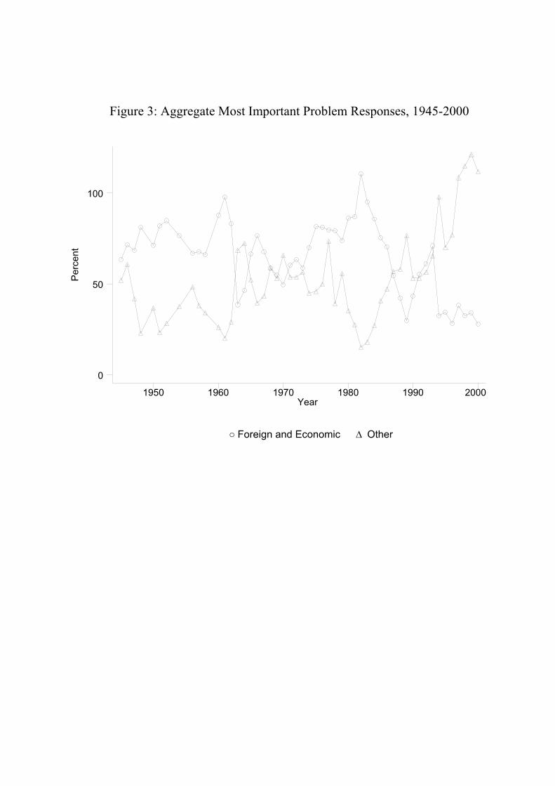
Figure 3: Aggregate Most Important Problem Responses, 1945-2000

Perc

ent

Year1950 1960 1970 1980 1990 2000

0

50

100

○ Foreign and Economic ∆ Other

Table 1. A Preliminary Analysis of Economic and Foreign Policy MIP Responses, 1973-2000 -------------------------------------------------------------------------------------- MIP Mentions (Percentage of Respondents) Independent Variable Economic Foreign -------------------------------------------------------------------------------------- Intercepta 36.46** 8.44** (7.22) (2.25) Economict-1 0.44** --- (0.11) Foreignt-1 --- 0.34* (0.14) Leading Economic 1.27** --- Indicatorst (inverted) (.25) Net Dislike of Russiat --- 0.08* (.03) R-squared .83 .47 Adjusted R-squared .81 .43 Standard Error 9.34 5.70 Durbin-Watson 1.79 1.50 N = 28, ** p < .01 * p < .05 (two-tailed) -------------------------------------------------------------------------------------- Note: The numbers in parentheses are standard errors. a Intercepts reflects the effects of the mean values of Leading Economic Indicators and Net Dislike of Russia.

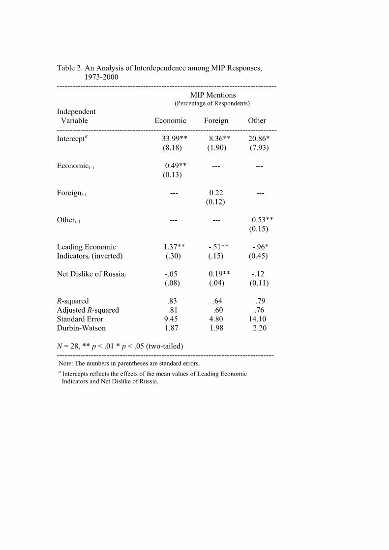
Table 2. An Analysis of Interdependence among MIP Responses, 1973-2000 ------------------------------------------------------------------------------------ MIP Mentions (Percentage of Respondents) Independent Variable Economic Foreign Other ------------------------------------------------------------------------------------ Intercepta 33.99** 8.36** 20.86* (8.18) (1.90) (7.93) Economict-1 0.49** --- --- (0.13) Foreignt-1 --- 0.22 --- (0.12) Othert-1 --- --- 0.53** (0.15) Leading Economic 1.37** -.51** -.96* Indicatorst (inverted) (.30) (.15) (0.45) Net Dislike of Russiat -.05 0.19** -.12 (.08) (.04) (0.11) R-squared .83 .64 .79 Adjusted R-squared .81 .60 .76 Standard Error 9.45 4.80 14.10 Durbin-Watson 1.87 1.98 2.20 N = 28, ** p < .01 * p < .05 (two-tailed) ----------------------------------------------------------------------------------- Note: The numbers in parentheses are standard errors. a Intercepts reflects the effects of the mean values of Leading Economic Indicators and Net Dislike of Russia.

Table 3. On the Structure of “Foreign Affairs” Responses, 1973-2000 -------------------------------------------------------------------------------------- MIP Mentions (Percentage of Respondents) Independent Variable Defense International -------------------------------------------------------------------------------------- Intercepta -.16 4.15** (1.12) (1.35) Defenset-1 0.43** ---

(0.09) Internationalt-1 --- 0.16 (0.20) Leading Economic -.44** .01 Indicatorst (inverted) (.11) (.11) Net Dislike of Russiat 0.16** -.01 (.03) (.03) R-squared .81 .05 Adjusted R-squared .78 -.07 Standard Error 3.64 3.64 Durbin-Watson 1.59 1.98 N = 28, ** p < .01 * p < .05 (two-tailed) -------------------------------------------------------------------------------------- Note: The numbers in parentheses are standard errors.

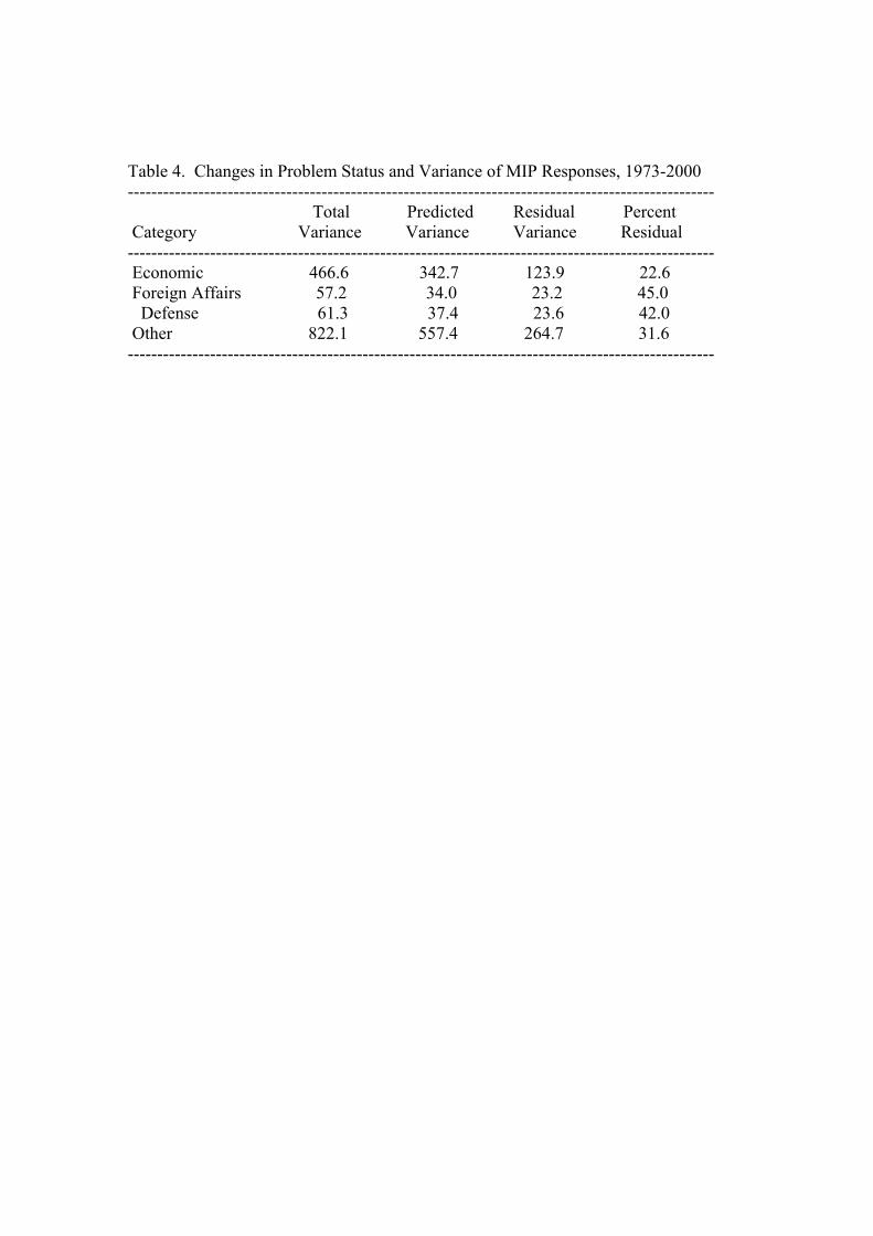
Table 4. Changes in Problem Status and Variance of MIP Responses, 1973-2000 ---------------------------------------------------------------------------------------------------- Total Predicted Residual Percent Category Variance Variance Variance Residual ---------------------------------------------------------------------------------------------------- Economic 466.6 342.7 123.9 22.6 Foreign Affairs 57.2 34.0 23.2 45.0 Defense 61.3 37.4 23.6 42.0 Other 822.1 557.4 264.7 31.6 ----------------------------------------------------------------------------------------------------

Table 5. Defense Spending Preference Regressions, 1974-1995a ------------------------------------------------------------------------------------------- Independent Variableb Basic With MIP With MIP* ------------------------------------------------------------------------------------------- Intercept 3.56* 3.45* 4.13** (1.82) (1.98) (1.56) Net Dislike of 0.51** 0.53** 0.48** the Soviet Uniont (0.11) (0.12) (0.14) (differenced) Net Dislike of 0.39** 0.41** 0.42** the Soviet Uniont-1 (0.12) (0.13) (0.14) (differenced) Defense Appropriationst -.68** -.72** -.92** (differenced) (0.13) (0.21) 0.26) Defense MIPt --- 0.16 --- (0.25) Defense Appropriationst --- 0.00 --- (differenced) * Defense MIPt (0.02) Defense MIP*

t --- --- -.14 (0.45) Defense Appropriationst --- --- 0.03 (differenced) * Defense MIP*

t (0.03) R-squared .75 .75 .77 Adjusted R-squared .67 .63 .65 Standard Error 7.84 8.25 8.08 Durbin-Watson 2.03 1.95 1.73 N=22, * p<.05, ** p<.01 (one-tailed) -------------------------------------------------------------------------------------------- Note: The numbers in parentheses are standard errors. a Results are based on estimated models that include controls for the Kuwait-Iraq crisis. b All independent variables are mean-centered.

Table 6. Defense Appropriations Regression, Fiscal Years 1974-1995, in Billions of 1987 Dollarsa --------------------------------------------------------------------------------------------- Independent Variableb Basic With MIP With MIP* ---------------------------------------------------------------------------------------------- Intercept 11.38** 11.48** 16.55** (2.80) (3.01) (4.28) Democratic -11.00* -10.96* -10.60* Presidentt-1 (5.26) (5.55) (5.11) Democratic -.21 -.11 -.42 Composition (0.53) (0.64) (0.56) of Congresst-1 Net Support for 0.66** 0.66** 0.85** Defense Spendingt-1 (0.10) (0.10) (0.19) Defense MIPt-1 --- 0.23 --- (0.44) Net Supportt-1 * Defense MIPt-1 --- 0.02 --- (0.03) Defense MIP*

t-1 --- --- 0.56 (0.77) Net Supportt-1 * Defense MIP*

t-1 --- --- 0.05 (0.03) R-squared .74 .74 .78 Adjusted R-squared .68 .64 .70 Standard Error 8.50 8.93 8.23 Durbin-Watson 1.95 2.12 2.47 N=22, * p<.05, ** p<.01 (one-tailed) ---------------------------------------------------------------------------------------------- Note: The numbers in parentheses are standard errors. a Results are based on estimated models that include a control for the Kuwait-Iraq crisis in fiscal year 1992. b All independent variables are mean-centered.