On the quality of measured optical aberration coefficients using phase wheel monitor

Lena V. Zavyalova*, Aaron R. Robinson, Anatoly Bourov, Neal V. Lafferty, and Bruce W. Smith

Center for Nanolithography Research Rochester Institute of Technology, 82 Lomb Memorial Drive, Rochester NY 14623, USA

ABSTRACT

In-situ aberration measurement often requires indirect methods that retrieve the pupil phase from the measured images and presents unique challenges to the engineers involved. Phase wheel monitor allows such in-situ measurement of aberrations in photolithography systems. The projection lens aberrations may be obtained with high accuracy from images of phase wheel targets printed in photoresist. As a result, the photolithography tool optics can be characterized under standard wafer printing conditions. Resulting features are mathematically analyzed to extract information about the aberrations in optics. We use a detection algorithm and multi-domain modeling to process resist images and determine the image deviation from the ideal shape, which in turn allow the amount of aberration introduced by the optical system to be quantified. Experimental results are shown and multiple measurements on the same tool before and after system corrections are compared. Keywords: Phase wheel monitor, aberrations, lithography, wavefront, Zernike polynomials

1. INTRODUCTION This imaging problem deals with images that have been degraded by the presence of aberrations as well as by the limited resolution of the system. The resolution is limited by diffraction and other sources that are well understood. To understand the impact of aberrations, the optical system, in the coherent case, can be characterized by way of the point spread function (PSF). The point spread function describes the optical system response to an impulse or a δ-function. The PSF has a specific character based on the aberration present. Figure 1 shows the system PSF obtained based on the point as object. It is noted that different aberrations produce different impulse response. Analogously to PSF, the argument can be made that the ring spread function (RSF) describes the system’s response to a given ring target. This function is similar to the point spread function, instead using a ring-δ function as the system input. It also has a unique character based on the aberration type, magnitude, and sign. Figure 2 shows how RSF relates to image quality when aberrations are present. For instance, coma aberration, known to cause pattern asymmetry and pattern shifts, affects the ring images in its characteristically unique way.

* lvzemc@rit.edu; phone 1 585 475 7991; fax 1 585 475 5041; www.rit.edu/lithography

Fig. 1. Coherent system PSF for a point object in the presence of 3-foil, astigmatism, and coma aberration.

Fig. 2. A radial arrangement of ‘ring’ spread functions for the multiple ring-delta-like objects: ideal unaberrated (left) vs. coma-only aberration (right).

2. PHASE WHEEL ABERRATION MONITOR The phase wheel aberration target is shown in Figure 3. On the photomask (Figure 3, left), it is a transparent pattern of nine radially arranged circular zones—a phase wheel—each π phase shifted relative to the background. The 0-to-180 degree phase transitions on the mask print as rings into the photoresist, yielding a set of RSFs. Figure 3 (right) shows the top-down SEM image of phase wheel target on the wafer, indicative of the aberration effects. Different target zones exhibit different response to aberration.

Fig. 3. Typical Phase Wheel target on a two level 0/π phase shift mask (left) and its image that results on the photoresist coated wafer (right).

3-point Coma Astigmatism

The target features are typically sized in ranges between 0.5 and 1.5 λ/NA and the entire phase wheel target is between 2.5 and 5 λ/NA in size. The phase wheel test implementation is made possible through the use of a standard phase shift mask with the chromeless π-phase shifted regions defining the test object structure in complex amplitude. Further, the test implementation requires producing a varying phase signal at the image plane. One of these images (and the spread function) is the in-focus image that has been degraded by the unknown aberrations. Additional images of the same object are formed by perturbing these aberrations with a known amount of phase error such as defocus. The relative phase difference introduced between the wavefronts is encoded within the spread function signal of each. The test is run during a standard operation of a lithography system in the Focus-Exposure Matrix mode, where the phase wheel target is projected onto a wafer image plane where it is captured in photoresist and evaluated.

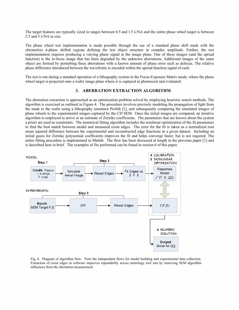
3. ABERRATION EXTRACTION ALGORITHM The aberration extraction is approached as an optimization problem solved by employing heuristic search methods. The algorithm is exercised as outlined in Figure 4. The procedure involves precisely modeling the propagation of light from the mask to the wafer using a lithography simulator Prolith [1], and subsequently comparing the simulated images of phase wheels to the experimental images captured by the CD SEM. Once the initial images are compared, an iterative algorithm is employed to arrive at an estimate of Zernike coefficients. The parameters that are known about the system a priori are used as constraints. The numerical fitting algorithm includes the nonlinear optimization of the fit parameters to find the best match between model and measured resist edges. The error for the fit is taken as a normalized root mean squared difference between the experimental and reconstructed edge functions in a given dataset. Including an initial guess for Zernike polynomial coefficients improves the fit and helps converge faster, but is not required. The entire fitting procedure is implemented in Matlab. The flow has been discussed at length in the previous paper [1] and is described here in brief. The examples of fits performed can be found in section 6 of this paper.

Fig. 4. Diagram of algorithm flow. Note the independent flows for model building and experimental data collection. Extraction of resist edges in software improves repeatability across metrology tool sets by removing SEM algorithm influences from the aberration measurement.

The experimental part of the phase wheel procedure involves the generation of a focus-exposure (FE) matrix wafer. The user performs experiment, collects the SEM data, and feeds the images into the Phase Wheels software (which is described in more detail in the next section) for image processing and analysis.

4. USING PHASE WHEEL IMAGE ANALYSIS SOFTWARE: FITTING AND ANALYSIS The Phase Wheels software program was developed in Matlab [3] with the goal to easily define models, gather data, automate data processing, manage model formulations, analyze results, and perform visualization tasks. At present the software implements several key steps of the algorithm. The initial step of dataset generation, which processes the SEM images, extracts and measures features, and further parameterizes the feature edges, is designed to work with several different SEM tool types. The next step it the dataset calibration which is based on parameters of the dataset that are independent of aberrations. Finally, the fitting of the dataset to the supplied model is performed. The output of this is a visualized wavefront along with the predicted Zernike values.

Fig. 5. Phase Wheel software environment during image analysis stage of phase wheel SEM with corresponding extracted Bossung plot and response surface model calibration The software includes the SEM image analysis feature to verify and predict the Focus/Dose performance of phase wheel targets (shown in Figure 5). The main goals are to visualize the effects of exposure, defocus, and aberrations on the target’s image.

The image analyzer is a valuable tool for visualizing the ED-window of the test target and parameters used to describe the edges in the test target, such as ring radius, width, etc., from hereon referred to as phase wheel target parameters. Each SEM picture is parameterized and analyzed as a function of exposure, defocus, and aberration, as demonstrated in Figure 5. The edges are extracted, denoised, and superimposed over the SEM image. This is also a quick sanity check for the user to ensure that the images being fed into the system are being processed correctly. Software panels with multiple custom options to achieve optimal fit to the data are present and let the user to define the models and specify how the fit should be performed. Simple operations for comparison of wavefront from multiple sources are also built-in. The user may define specific wavefronts to visualize and compare against fitted data as well as save those wavefronts for future comparisons and importing them into other programs. In addition to various wavefront inspection options, the phase wheel software provides the broad range of features and visualizations, including familiar Bossung-type output, that consolidate large amounts of information and facilitate the model building process.

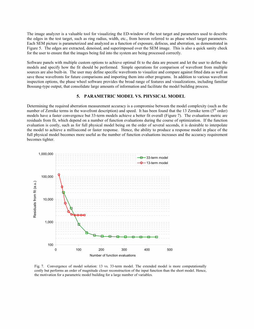
5. PARAMETRIC MODEL VS. PHYSICAL MODEL Determining the required aberration measurement accuracy is a compromise between the model complexity (such as the number of Zernike terms in the wavefront description) and speed. It has been found that the 13 Zernike term (5th order) models have a faster convergence but 33-term models achieve a better fit overall (Figure 7). The evaluation metric are residuals from fit, which depend on a number of function evaluations during the course of optimization. If the function evaluation is costly, such as for full physical model being on the order of several seconds, it is desirable to interpolate the model to achieve a millisecond or faster response. Hence, the ability to produce a response model in place of the full physical model becomes more useful as the number of function evaluations increases and the accuracy requirement becomes tighter.

100

1,000

10,000

100,000

1,000,000

0 100 200 300 400 500

Number of function evaluations

Res

idua

ls fr

om fi

t (a.

u.)

33-term model13-term model

Fig. 7. Convergence of model solution: 13 vs. 33-term model. The extended model is more computationally costly but performs an order of magnitude closer reconstruction of the input function than the short model. Hence, the motivation for a parametric model building for a large number of variables.

To replace costly simulations, design of experiments theory and response surface modeling are used to build compact polynomial response surface models that describe lithographic imaging of the phase wheels. The focus, dose, and Zernike coefficients are variables, and phase wheel edges are the modeled responses. In addition to faster computation (1 msec vs. 5 sec), the advantage of response model over the full physical model is that the important contributions from the multitude of variables can be easily identified. And once they are built, they are easy to use and distribute, without additional need for the full lithography simulator. By their nature, the interpolating models are accurate within the specified design space only. For example, the useable focus range is ±λ/NA2, exposure range may be ±12.5% from the nominal dose; Z4-Z36 aberration coefficients might each be within 50 mwaves; a single NA and σ setting applies. The nonlinear optimization will set the constraints based on these variables values when solving for aberration coefficients. Focus and dose have to be calibrated for each photoresist process; therefore a calibration model is built along with each fit model. Calibration is automatically performed every time a dataset is analyzed. In its most general form, the parametric model equation with n inputs is: ( ) β β β β β β ε

> > >

= + + + + + + +∑ ∑∑ ∑ ∑∑∑ ∑ KK2

0 , , ,; nj j jk j k jj j jkl j k l j j j j

j j k j j j k j l k j

f x x x x x x x xx β ,

where x is a vector of predictors and β is a vector of model coefficients.

Fig. 6. Example response model surface is viewed in three dimensions vs. calibrated focus (µm) and dose correctable. The dots are experimentally obtained points, which are in close agreement with the computed model of data (surface).

In Figure 6, model parameterization is visualized to the user in 3 dimensions and serves as the fit diagnostic tool. It demonstrates the use of a quadratic polynomial response surface to approximate the extracted signal from the phase wheel. Plotted on the z-axis is one of the many a parameters used to describe the printed target. The response model provides a good estimation for the chosen coefficient. Furthermore, such low-dimensional model representation is fairly simple and intuitive to the lithographer accustomed to working with the Bossung plots. It is implied however that when the number of model parameters grows large, other metrics and/or tests become useful in quantifying statistical significance of parameter estimates for the models. These more specialized diagnostics are also available to the user via the report generation options inside the phase wheels software.

6. MODEL VERIFICATION The model verification has been performed to better understand the capabilities of models of varying complexity.

-0.15 -0.1 -0.05 0 0.05 0.11.25

1.3

1.35

1.4

1.45

1.5-75

-70

-65

-60

-55

-50

Focus

Dose

Z

Wavefront analysis tool in phase wheels software allows the user to run a comparison of two fitted wavefronts, as illustrated in Figure 8. The pupil of Figure 8 had Z4-Z36 aberrations. Fitted wavefront surface using 13 Zernike coefficients (top left) is compared to wavefront fitted with 22 Zernike terms (top right). Both models provide a reasonable fit to the data, as the difference plot between the two wavefronts (bottom left) shows. The fit differences are mainly in the outer portion of the pupil, which highlights the need to include high-order Zernike polynomial terms in the wavefront description [4]. Also in Figure 8, a direct comparison for each coefficient is made with original wavefront (bar plot bottom right). The coefficients predicted with the 22-term model more closely match the actual coefficients.

Fig. 8. Single target fit to 13 and 22 Zernike-term models (λ=193nm, NA=0.85). The 13-term model predicts Z4-Z16 coefficients, while the 22-term model operates on Z4-Z25 coefficients. Fringe Zernike numbering scheme is used.

In the next case (shown in Figure 9), the goal was to detect and quantify a third order astigmatism Z5 term that was adjusted on the tool and compare wavefronts before and after correction. Most of the contribution from the low order astigmatism term (Z5) will come as orientation dependent best focus position and can result in the horizontal to vertical CD difference; hence, the Z5 correction was desired. As depicted in Figure 9, the wavefront in the top left is before the correction, and in the top right is the fitted wavefront after the Z5 correction. The fifth order 13 term (Z4-Z16) model was used to fit the data from three different phase wheel targets simultaneously. The fit results from both settings are consistent except for Z5 astigmatism where there is a 0.01 wave delta observed. The difference between the two wavefronts (bottom left) highlights the astigmatism signature that has been successfully removed upon the lens adjustment.

Fig. 9. Tool characterization and correction using Phase Wheels (λ=193nm, NA=0.85). Settings 1 and 2 correspond to fitted wavefronts sampled before and after correction, respectively.

7. SUMMARY We have presented our latest progress on the phase wheel aberration extraction method. The method has been speed optimized using a compact parametric response surface model in conjunction with optical lithography simulation. Furthermore, several improvements on the edge extraction algorithm have been realized, allowing more reliable, robust detection for a variety of SEM tools and increased accuracy. A stand-alone aberration analysis application has been developed in Matlab that supports the entire phase wheel analysis process and provides a flexible environment for the large-scale problems that we model. The wavefronts have been fit using up to 36 Zernike terms, incorporating image processing, calibration, edge extraction and wavefront surface fitting. Better than 0.7 nm (0.0035 λ) of accuracy with less than 0.4 nm (0.002 λ) of repeatability at 193 nm in photoresist has been achieved.

ACKNOWLEDGEMENTS The authors would like to acknowledge the support of Benchmark Technologies and TI. The authors would also like to gratefully acknowledge KLA-Tencor Corp. for donating the Microelectronic Engineering Department at RIT PROLITH™ lithography software licenses.

REFERENCES 1. Lithography simulator PROLITH™ v. 9.3 by KLA-Tencor. 2. Zavyalova L., Smith B., Bourov A., Zhang G., Vellanki V., Reynolds P., Flagello D. “Practical approach to full-

field wavefront aberration measurement using phase wheel targets,” Proc. SPIE, 6154, 2006. 3. MATLAB v.7.2, The MathWorks Inc., Natick, MA. 4. Zavyalova L., Bourov A., Smith B. “Automated aberration extraction using phase wheel targets,” Proc. SPIE,

5754, 2005.