ON THE EXTRACTION OF THE STRONG COUPLING CONSTANT FROMHADRONIC TAU DECAY

A Thesis Submitted to the Faculty ofSan Francisco State University

In Partial Fulfillment ofThe Requirements for

The Degree

Master of ScienceIn

Physics

by

James Alexander Osborne

San Francisco, CA

August 2011

Copyright by

James A. Osborne

2011

Certification of Approval

I certify that I have read On the Extraction of the Strong Coupling Constant from

Hadronic Tau Decay by James Alexander Osborne, and that in my opinion this

work meets the criteria for approving a thesis submitted in partial fulfillment of the

requirements for the degree: Master of Science in Physics at San Francisco State

University.

Dr. Maarten Golterman

Professor of Physics

Dr. Santiago Peris

Professor of Physics

Dr. Andisheh Mahdavi

Professor of Physics

On the Extraction of the Strong Coupling Constant from HadronicTau Decay

James Alexander OsborneSan Francisco, California

2011

We discuss the extraction of the strong coupling constant αs using hadronic τ

decay data. We examine the effects of duality violations and other systematic un-

certainties on the analysis of this data, and propose a more comprehensive method

of analysis which accounts for such uncertainties. We conclude that the presence

of these systematic uncertainties has a non-negligible effect on the analysis of

hadronic τ decay. Preliminary results correspond to αs(M2Z) = 0.1193 ± 0.0038

using contour-improved perturbation theory and αs(M2Z) = 0.1166± 0.0023 using

fixed order perturbation theory.

I certify that the Abstract is a correct representation of the content of this thesis.

Chair, Thesis Committee Date

This page intentionally left blank.

Acknowledgements

First and foremost I must express my gratitude to my adviser Dr. Maarten Golterman,

without whom this thesis would not be possible. His dedication to the advancement of my

education beyond the scope of coursework has truly enriched my life, and it has been both

a privilege and a joy to work with him.

I wish to thank my collaborators: Diogo Boito, Oscar Cata, Matthias Jamin, Kim Maltman,

and Santi Peris. Their continuing encouragement of my contributions to this project has

enabled me to succeed.

I wish to thank the faculty of the physics and astronomy department at San Francisco State

University for their unyielding commitment to quality education.

I wish to thank my family for their emotional and financial support. I would especially like to

recognize my mother and father, Thomas and Judith Osborne, as well as my grandmother,

Helen Brock, for enabling me to pursue my dreams.

Finally, I wish to thank the uncountable number of people who have provided friendship

throughout my life. I am indebted to you all for keeping me sane.

v

Table of Contents

List of Tables . . . . . . . . . . . . . . . . . . . . . . . . . . . . . . . . . . . . . . . . . . . . . . . . . . . . . . . . . . . . . . viii

List of Figures . . . . . . . . . . . . . . . . . . . . . . . . . . . . . . . . . . . . . . . . . . . . . . . . . . . . . . . . . . . . . ix

1. Introduction . . . . . . . . . . . . . . . . . . . . . . . . . . . . . . . . . . . . . . . . . . . . . . . . . . . . . . . . . . . . 1

2. Theoretical Framework . . . . . . . . . . . . . . . . . . . . . . . . . . . . . . . . . . . . . . . . . . . . . . . . . . 2

2.1. Tau Decay . . . . . . . . . . . . . . . . . . . . . . . . . . . . . . . . . . . . . . . . . . . . . . . . . . . . . . . . 4

2.2. Perturbation Theory . . . . . . . . . . . . . . . . . . . . . . . . . . . . . . . . . . . . . . . . . . . . . . 7

2.3. Operator Product Expansion . . . . . . . . . . . . . . . . . . . . . . . . . . . . . . . . . . . . . 10

3. Duality Violations . . . . . . . . . . . . . . . . . . . . . . . . . . . . . . . . . . . . . . . . . . . . . . . . . . . . . . 11

3.1. The Model . . . . . . . . . . . . . . . . . . . . . . . . . . . . . . . . . . . . . . . . . . . . . . . . . . . . . . . 12

3.2. Duality Violation Ansatz . . . . . . . . . . . . . . . . . . . . . . . . . . . . . . . . . . . . . . . . . 13

4. The “km” Spectral Analysis . . . . . . . . . . . . . . . . . . . . . . . . . . . . . . . . . . . . . . . . . . . . . 15

4.1. Systematic Errors . . . . . . . . . . . . . . . . . . . . . . . . . . . . . . . . . . . . . . . . . . . . . . . . . 16

5. Data . . . . . . . . . . . . . . . . . . . . . . . . . . . . . . . . . . . . . . . . . . . . . . . . . . . . . . . . . . . . . . . . . . . . 18

6. Fitting Strategies . . . . . . . . . . . . . . . . . . . . . . . . . . . . . . . . . . . . . . . . . . . . . . . . . . . . . . . 19

6.1. Correlated Fits . . . . . . . . . . . . . . . . . . . . . . . . . . . . . . . . . . . . . . . . . . . . . . . . . . . 22

6.2. Diagonal Fits . . . . . . . . . . . . . . . . . . . . . . . . . . . . . . . . . . . . . . . . . . . . . . . . . . . . . 23

6.3. Other Strategies . . . . . . . . . . . . . . . . . . . . . . . . . . . . . . . . . . . . . . . . . . . . . . . . . . 24

7. Fits . . . . . . . . . . . . . . . . . . . . . . . . . . . . . . . . . . . . . . . . . . . . . . . . . . . . . . . . . . . . . . . . . . . . . 25

7.1. Fits to w0(x) . . . . . . . . . . . . . . . . . . . . . . . . . . . . . . . . . . . . . . . . . . . . . . . . . . . . . 26

7.2. Combined Fits to w0(x), w2(x), and w3(x) . . . . . . . . . . . . . . . . . . . . . . . . 31

vi

7.3. Fits Excluding Duality Violations . . . . . . . . . . . . . . . . . . . . . . . . . . . . . . . . . 34

8. Summary of Results . . . . . . . . . . . . . . . . . . . . . . . . . . . . . . . . . . . . . . . . . . . . . . . . . . . . 35

9. Conclusion . . . . . . . . . . . . . . . . . . . . . . . . . . . . . . . . . . . . . . . . . . . . . . . . . . . . . . . . . . . . . . 37

Appendix A. Linear Fluctuation Analysis . . . . . . . . . . . . . . . . . . . . . . . . . . . . . . . . . . 38

References . . . . . . . . . . . . . . . . . . . . . . . . . . . . . . . . . . . . . . . . . . . . . . . . . . . . . . . . . . . . . . . . . 39

vii

List of Tables

Table Page

1 Vector channel fits for w0 . . . . . . . . . . . . . . . . . . . . . . . . . . . . . . . . . . . . . . . . . . . . . . . . . . 27

2 Axial-vector channel fits for w0 . . . . . . . . . . . . . . . . . . . . . . . . . . . . . . . . . . . . . . . . . . . . . 29

3 Combined vector and axial-vector channel fits for w0 . . . . . . . . . . . . . . . . . . . . . . . 30

4 Vector channel diagonal fits for w0,2,3 . . . . . . . . . . . . . . . . . . . . . . . . . . . . . . . . . . . . . . . 31

5 Vector channel block-diagonal fits for w0,2,3 . . . . . . . . . . . . . . . . . . . . . . . . . . . . . . . . . 32

6 Combined vector and axial-vector diagonal fits for w0,2,3 . . . . . . . . . . . . . . . . . . . . 34

7 Vector channel fits with no duality violation ansatz for w3 . . . . . . . . . . . . . . . . . . 35

viii

List of Figures

Figure Page

1 Dependence of αs on energy . . . . . . . . . . . . . . . . . . . . . . . . . . . . . . . . . . . . . . . . . . . . . . . . 3

2 Individual determinations of αs from ALEPH data . . . . . . . . . . . . . . . . . . . . . . . . . 4

3 Feynman diagrams for τ decay . . . . . . . . . . . . . . . . . . . . . . . . . . . . . . . . . . . . . . . . . . . . . 5

4 The optical theorem . . . . . . . . . . . . . . . . . . . . . . . . . . . . . . . . . . . . . . . . . . . . . . . . . . . . . . . 6

5 Finite energy sum rule contour . . . . . . . . . . . . . . . . . . . . . . . . . . . . . . . . . . . . . . . . . . . . . 8

6 OPAL data compared to our model . . . . . . . . . . . . . . . . . . . . . . . . . . . . . . . . . . . . . . . . 13

7 Duality violation contour . . . . . . . . . . . . . . . . . . . . . . . . . . . . . . . . . . . . . . . . . . . . . . . . . . 14

8 OPAL data versus perturbation theory . . . . . . . . . . . . . . . . . . . . . . . . . . . . . . . . . . . . . 17

9 OPAL and ALEPH correlations . . . . . . . . . . . . . . . . . . . . . . . . . . . . . . . . . . . . . . . . . . . . 18

10 OPAL spectral function data . . . . . . . . . . . . . . . . . . . . . . . . . . . . . . . . . . . . . . . . . . . . . . . 20

11 OPAL data versus OPE + DV theory for w0 . . . . . . . . . . . . . . . . . . . . . . . . . . . . . . . 28

12 Integrated OPAL data versus OPE + DV theory for w3 . . . . . . . . . . . . . . . . . . . . 33

ix

List of Appendices

Appendix Page

A. Linear Fluctuation Analysis . . . . . . . . . . . . . . . . . . . . . . . . . . . . . . . . . . . . . . . . . . . . . . . . 38

x

1

1. Introduction

Quantum Chromodynamics (QCD) is the standard model theory of strong interac-

tions, which describes the generation of the majority of visible mass in our universe.

It is a theory of quarks, which bind together to form hadrons such as protons and

neutrons, and gluons, a massless force mediating boson. QCD predicts that the po-

tential between quarks increases linearly as a function of distance. For this reason,

individual quarks and gluons do not exist in nature and only their hadronic bound

states are directly observed. The belief that a theory of quarks and gluons accurately

describes observable hadronic physics goes by the name of quark-hadron duality, and

our ability to calculate physics from QCD is an important test of this duality.

The strong coupling constant αs is the fine structure constant equivalent of QCD,

and it governs the strength of strong interactions. As an input parameter in the

standard model, it is important to have a precise determination of the value of αs.

High precision determinations benefit not only our current understanding of particle

physics, but also aid in the search for theories of physics beyond the standard model

such as grand unification. The value of αs grows as a function of distance to match

to the predicted strength of quark interactions. In fact, QCD is asymptotically free:

the value of αs approaches zero at very short distances, or, equivalently, at very high

energies after a Fourier transformation. This allows us to employ QCD perturbation

theory to analyze high-energy processes, which then makes it possible to measure αs

directly.

It has been known for some time that hadronic decays of the tau lepton (τ) can

lead to a relatively clean extraction of the strong coupling constant [1]. The mass

of the τ (mτ = 1.78 GeV) is large enough that perturbative expressions can ac-

curately describe the physics of its decay with only small corrections coming from

non-perturbative contamination. This then makes it possible to obtain a value for

αs from experimental measurements. Currently, the most precise experimental deter-

minations of αs come from experiments performed by the ALEPH [2] and OPAL [3]

collaborations at CERN’s LEP collider.

2

This paper introduces a new framework for the analysis of hadronic τ decay in

which we examine previously unquantified systematic errors. In section 2 we present

a summary of the theoretical background employed to isolate αs from τ decay. In

section 3 we discuss the development of a model for “duality violations,” a systematic

error unaccounted for in all previous τ decay analyses. In section 4 we give an overview

of prior analysis methods, and discuss the major systematic errors involved. In section

5 we discuss currently available hadronic τ decay data, and in section 6 we introduce a

more comprehensive strategy for extracting αs from this data. In section 7 we present

the results of fits to this data, and in section 8 we offer our conclusion regarding the

best available fitting strategy. Additionally, we present preliminary values for αs

based on this new method of analysis.

2. Theoretical Framework

The research discussed here involves determining the value of αs. Following con-

vention, the coupling constant is extracted after renormalization, at the τ mass, and

in the modified minimal subtraction (MS) regularization scheme. Figure 1 shows the

dependence of αs on energy. The data points depicted are select experimental deter-

minations, shown at the natural mass of each experiment, along with the theoretical

lattice QCD determination. The yellow band shows the QCD prediction, with the

central value and errors given by the world average of αs. At the Z mass this is [4]

αs(M2z ) = 0.1184± 0.0007 . (2.1)

It should be noted that the errors associated with these determinations of αs also

scale according to energy, so that precise determinations at low energies become even

more precise when scaled up to higher energies.

Hadronic τ decay currently claims the most precise experimental determination

of αs. Because of the relatively low mass of the τ (mτ = 1.78 GeV), precision

determinations at this energy scale compete with determinations at much higher

energies (MZ = 91.19 GeV) with the appropriate scaling of errors. Determinations

of αs(m2τ ) from hadronic τ decay using contour-improved perturbation theory (cf.

3

Figure 1. A summary of αs as a function of energy. Select experi-mental results are shown at the natural mass of each experiment. Thecurves shown represent the QCD predictions given by the world averagevalue of αs. (Figure from reference [4].)

section 2.2) provided

αs(m2τ ) = 0.345± 0.004exp ± 0.009th (ALEPH [2]),

αs(m2τ ) = 0.348± 0.009exp ± 0.019th (OPAL [3]). (2.2)

These determinations are on the high side of the world average, which is currently

dominated by the lattice QCD computation. Understanding the disparity between

results from τ decay and lattice QCD represents an important test of QCD’s ability

to accurately describe fundamental physics.

More importantly, determinations of αs from the same experimental data by differ-

ent groups do not agree within their respective errors (see Figure 2). The discrepancies

arise from different choices of how to include both perturbative and non-perturbative

4

Figure 2. Determinations of αs from ALEPH [2] hadronic τ decaydata by [5, 6, 7, 8, 9, 10]. The dashed line and yellow band show theaverage value and the inclusive error estimated for the 2009 world av-erage. (Figure from reference [4].)

effects. Although the correlations between data points may have been significantly

underestimated (cf. section 5), it is vital to understand the underlying mechanism

behind these variations. Here, we will present an analysis of the systematic errors

present in these determinations in an attempt to come up with a more comprehensive

framework for the analysis of τ decay.

2.1. Tau Decay. The analysis of hadronic τ decay begins with the ratio of its decay

rate into hadrons to its decay rate into electrons,

Rτ ≡Γ[τ− → ντ hadrons]

Γ[τ− → ντ e− νe]. (2.3)

The τ decays through the weak interaction into a τ neutrino and aW boson (Figure 3).

The W in turn can decay into either leptons – an electron and anti-electron neutrino

pair, or a muon and anti-muon neutrino pair – or hadrons – an anti-up and down quark

pair (ud), or an anti-up and strange quark pair (us). Heavier quark production is

excluded by energy conservation, and other possible quark combinations are excluded

due to charge considerations. These quark anti-quark pairs can then interact strongly

through the exchange of gluons, which allows us to extract QCD-related information.

Experimentally, the ratio (2.3) can be decomposed into non-strange and strange

quark current contributions. The non-strange contribution can be further decomposed

5

a) decay to electrons:

b) decay to hadrons:

+ + . . .

Figure 3. Feynman diagrams depicting tau decay through weak in-teractions into a) electrons and associated neutrinos, and b) quark-antiquark pairs.

into vector and axial-vector components, so that we can write Rτ = RVud +RA

ud +Rus.

Only the non-strange contributions are typically analyzed in the extraction of αs

because analysis of the non-strange interactions involves only the lightest quarks,

whose masses can safely be neglected in perturbative calculations. Exclusion of Rus

provides a cleaner analysis by removing the error associated with the value of ms.

We define the two-point correlation functions of the non-strange quark currents as

ΠµνV,A ≡ i

∫d4x eiq·x〈0|T{JµV,A(x)J† νV,A(0)}|0〉

= (qµqν − q2gµν)Π(1)V,A(q2) + qµqνΠ

(0)V,A(q2), (2.4)

where JµV (x) = u(x)γµd(x) and JµA(x) = u(x)γµγ5d(x). The superscript J = 1, 0

denotes the angular momentum in the hadronic rest frame. By use of the optical

theorem (Figure 4), equation (2.3) can be expressed in terms of the imaginary parts

of these correlators, which are proportional to the experimentally accessible spectral

6

Figure 4. The optical theorem: the sum of all possible final state par-ticles equals the imaginary part of the shown scattering process.

functions as measured in τ decays. This gives [1]:

RV,Aτ = 12πSEW |Vud|2

∫ m2τ

0

ds

m2τ

(1− s

m2τ

)2 [(1 + 2

s

m2τ

)Im Π

(1)V,A(s) + Im Π

(0)V,A(s)

],

(2.5)

where SEW is a short-distance electroweak correction and Vud is the ud CKM matrix

element. The polynomials in the integrand come from kinematic considerations and

s = q2 is the total energy of the final state hadrons. In the initial decay process

τ → ντ +W , the τ neutrino can take away any amount of energy between 0 and m2τ .

The energy of the final state hadrons must then be integrated over, since the off-shell

W boson can carry any energy between 0 ≤ s ≤ m2τ .

The individual spin components currently have not been separated experimentally.

However, we may rewrite equation (2.5) as

RV,Aτ = 12πSEW |Vud|2

∫ m2τ

0

ds

m2τ

(1− s

m2τ

)[(1 + 2

s

m2τ

)Im Π

(1+0)V,A (s)− 2

s

m2τ

Im Π(0)V,A

].

(2.6)

All contributions to the J = 0 term are numerically negligible, apart from a contri-

bution to the axial-vector channel due to the pion bound state [2, 3]. The measured

data does not contain this contribution, and so its estimated value must be added to

the axial-vector spectral function. We will show the details of this calculation below.

The spectral functions ρV,A(s) = (1/π) Im Π(1+0)V,A are physically measured. Because

of this, we are not confined to the specific form of the integrand in equation (2.6). We

may instead replace the kinematic weight with an arbitrary polynomial. Additionally,

7

the only significant contribution to the second term comes from the pion, which is

not included in the experimental determinations. We therefore drop this term and

consider the general “moment”

RV,Aw = SEW |Vud|2

∫ s0

0

dsw(s)1

πIm Π

(1+0)V,A (s) . (2.7)

Traditionally, w(s) = wτ (s) ≡ (12π2/s0)(1 − s/s0)2(1 + 2s/s0) and s0 = m2τ , but in

theory any polynomial w(s) may be employed since only ρV,A(s) ≡ 1/π Im ΠV,A(s) is

determined experimentally.

As mentioned above, the experimental data does not contain a contribution from

the π pole in the axial-vector channel which will therefore need to be added in. This

numerically significant term takes the form ρ(0)π (s) = 2 f 2

π δ(s−M2π), where fπ is the

pion decay constant. Inserting this expression into equation (2.7), we can isolate the

π pole contribution to the axial-vector spectral function to

RAw(s0, π) = 2SEW |Vud|2 f 2

π w(M2π) . (2.8)

As this is the only significant contribution to the J = 0 term, we will set it aside until

later and drop the J = 1 + 0 superscript on ΠV,A(s).

2.2. Perturbation Theory. Although the exact structure of the correlators ΠV,A(s)

is unknown, they have poles and branch cuts at momenta where the intermediate

states from the optical theorem exist, along the positive real s axis. Furthermore,

ΠV,A(s) can be expressed perturbatively as a power series expansion in αs, but only at

large s. The moment (2.7), however, requires evaluating ΠV,A(s) both on the positive

real s axis where it has a branch cut and at low energy where the perturbative

expression is not valid. We must therefore find an expression that relates equation

(2.7) to a region where ΠV,A(s) need only be evaluated at s � Λ2QCD away from the

positive real s axis.

Using Cauchy’s theorem and the analytic properties of the correlators, we can re-

express equation (2.7) in terms of a contour integral of radius |s| = s0. Integrating

w(s) Π(s) with Π(s) = ΠV,A(s) along the contour in figure 5, we arrive at the finite

8

Figure 5. FESR contour. The discrepancy across the cut is equal to 2i Im Π(s).

energy sum rule (FESR) [11]:∫ s0

0

dsw(s)1

π[Π(s+ iε)− Π(s− iε)] = − 1

π

∮|s|=s0

dsw(s) Π(s) ,

or∫ s0

0

dsw(s)1

πIm Π(s) = − 1

2πi

∮|s|=s0

dsw(s) Π(s). (2.9)

Above we have used the fact that Π(s∗) = Π∗(s). Using this, we can rewrite RV,Aw in

terms of a contour integral that allows us to both avoid the poles and cuts on the

positive real s axis and evaluate ΠV,A(s) at energies where the perturbative expres-

sions are valid. Rewriting equation (2.7) using equation (2.9) and the perturbative

approximation ΠV,A(s) ≈ ΠPTV,A, we have

RV,Aw ≈ −SEW |Vud|2

1

2πi

∮|s|=s0

dsw(s) ΠPTV,A(s) . (2.10)

9

In the limit of vanishing quark masses, the vector and axial-vector correlators have

identical perturbative expansions of the form [12]

ΠPT (s) = − 1

4π2

∞∑n=0

an(µ2)n+1∑k=0

cnk logk(− s

µ2

), (2.11)

where a(µ2) ≡ αs(µ2)/π and µ is the renormalization scale. The coefficients cnk have

been analytically determined up to n = 4 [7]. The scaling of αs(µ2) as a function of

energy is defined by the QCD β function

−µdadµ≡ β(a) = β1a

2 + β2a3 + β3a

4 + β4a5 + . . . , (2.12)

where the coefficients have been determined up to β4 [7].

As this section deals solely with the short distance perturbative effects of QCD, we

drop the PT subscript on Π(s) and define the Adler function as

D(s) ≡ −s dds

Π(s) =1

4π2

∞∑n=0

an(µ2)n+1∑k=1

k cnk logk−1(− s

µ2

). (2.13)

Although Π(s) itself is not a physical quantity, the spectral functions ρV,A(s) (because

they are measurable) and the Adler function D(s) (because the derivative removes

an unphysical infinite constant) are. Therefore, their values can not depend on the

renormalization scale µ, and we are free to choose any value for µ2 in expression

(2.13).

To simplify equation (2.10), we first express the right hand side in terms of the

physical Adler function by partial integration.

RPTw = −SEW |Vud|2

1

2πi

∮|s|=s0

ds

sW (s)D(s) ,

=SEW |Vud|2

8π3i

∮|s|=s0

ds

sW (s)

∞∑n=0

an(µ2)n+1∑k=1

k cnk logk−1(− s

µ2

), (2.14)

where w(s) ≡ ddsW (s) and W (s0) = 0. We can simplify this expression somewhat

through our choice of the renormalization scale µ. Two traditional choices are either

µ2 = s0, which goes by the name of fixed order perturbation theory (FOPT), or

10

µ2 = −s, which goes by the name of contour-improved perturbation theory (CIPT)

[8, 13, 14, 15].

We therefore have the following perturbative expressions for RV,Aw :

RFOw =

SEW |Vud|2

8π3i

∞∑n=0

an(s0)n+1∑k=1

k cnk

∮|s|=s0

ds

sW (s) logk−1

(− s

s0

), (2.15)

RCIw =

SEW |Vud|2

8π3i

∞∑n=0

cn1

∮|x|=1

ds

sW (s) an(−s) . (2.16)

These series must be truncated for any practical application, which creates differences

between the two expressions above. And although the truncated series are different

and thus lead to different values of αs, our goal is to focus on non-perturbative

systematics. We will therefore present both FOPT and CIPT results simultaneously

without attempting to reconcile the values we obtain by these two methods.

2.3. Operator Product Expansion. Because m2τ is relatively small and pertur-

bation theory is at best asymptotic, non-perturbative effects should be expected to

impact this analysis. One method to account for such effects is by including non-

perturbative corrections from the operator product expansion (OPE). The OPE takes

the form

Π(s) =∑

D=0,2,4,...

1

(−s)D/2∑

dimO=D

CD(s, µ) 〈O(µ)〉. (2.17)

The Wilson coefficients C(s, µ) can be expanded perturbatively in powers of αs. Thus

the D = 0 term in the OPE, with the unit operator being the only operator with

dimension 0, is given by perturbation theory. The dimension 2 operators take the

form mimj, where i(j) = u, d. Because mu,d are small, the D = 2 contributions to

the OPE may be neglected.

We will assume that the energy dependence of the Wilson coefficients is small in

the energy range of this analysis, so that it can be neglected. We can then express

the OPE in the form

ΠOPEV,A (s) = ΠPT

V,A(s) +C4

s2− C6

s3+C8

s4− C10

s5+ . . . , (2.18)

11

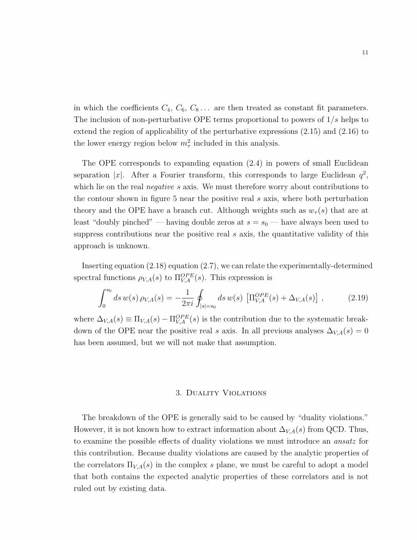
in which the coefficients C4, C6, C8 . . . are then treated as constant fit parameters.

The inclusion of non-perturbative OPE terms proportional to powers of 1/s helps to

extend the region of applicability of the perturbative expressions (2.15) and (2.16) to

the lower energy region below m2τ included in this analysis.

The OPE corresponds to expanding equation (2.4) in powers of small Euclidean

separation |x|. After a Fourier transform, this corresponds to large Euclidean q2,

which lie on the real negative s axis. We must therefore worry about contributions to

the contour shown in figure 5 near the positive real s axis, where both perturbation

theory and the OPE have a branch cut. Although weights such as wτ (s) that are at

least “doubly pinched” — having double zeros at s = s0 — have always been used to

suppress contributions near the positive real s axis, the quantitative validity of this

approach is unknown.

Inserting equation (2.18) equation (2.7), we can relate the experimentally-determined

spectral functions ρV,A(s) to ΠOPEV,A (s). This expression is∫ s0

0

dsw(s) ρV,A(s) = − 1

2πi

∮|s|=s0

dsw(s)[ΠOPEV,A (s) + ∆V,A(s)

], (2.19)

where ∆V,A(s) ≡ ΠV,A(s)−ΠOPEV,A (s) is the contribution due to the systematic break-

down of the OPE near the positive real s axis. In all previous analyses ∆V,A(s) = 0

has been assumed, but we will not make that assumption.

3. Duality Violations

The breakdown of the OPE is generally said to be caused by “duality violations.”

However, it is not known how to extract information about ∆V,A(s) from QCD. Thus,

to examine the possible effects of duality violations we must introduce an ansatz for

this contribution. Because duality violations are caused by the analytic properties of

the correlators ΠV,A(s) in the complex s plane, we must be careful to adopt a model

that both contains the expected analytic properties of these correlators and is not

ruled out by existing data.

12

3.1. The Model. The model we will adopt is that of a vector two-point correlator

which contains an infinite set of finite-width resonsances. This model was first sug-

gested in references [16, 17, 18] for the purpose of studying duality violations. The

version we will consider here was adapted in references [19, 20], and is given by

ΠV (s) =1

ζ

[2F 2

ρ

z +m2ρ

+∞∑n=0

2F 2

z +m2V (n)

+ constant

], (3.1)

where

z = Λ2

(−s− iε

Λ2

)ζ, ζ = 1− η , and m2

V (n) = m20 + nΛ2 .

Note that η is a small parameter such that ζ is close to unity, which corresponds

to narrow decay widths. Although a separate ρ resonance is included in the above

expression due to phenomenological considerations, its inclusion will not be relevant

for the developments that follow.

Equation (3.1) can be expressed in closed form as

ΠV (s) =1

ζ

[2F 2

ρ

z +m2ρ

− 2F 2

Λ2ψ

(z +m2

0

Λ2

)+ constant

], (3.2)

where ψ(z) = Γ′(z)/Γ(z) is the Euler digamma function. Using an asymptotic ex-

pansion of the digamma function,

ψ(z) = log z − 1

2z−∞∑n=1

B2n

2nz2n|z| � 1 , −π < arg(z) < π (3.3)

where B2n are the Bernoulli numbers, it is straightforward to obtain the OPE for this

model:

ΠOPEV (s) ≈ 2F 2

Λ2C0 log(−s) +

∞∑k=1

C2k

zk+ constant , (3.4)

where

C0 = 1 , C2k =2

ζ(−1)k

[−F 2

ρm2k−2ρ +

1

kΛ2k−2F 2Bk

(m2

0

Λ2

)](3.5)

and Bk(x) are the Bernoulli polynomials

Bn(x) =n∑k=0

(n

k

)Bk x

n−k . (3.6)

13

0.0 0.5 1.0 1.5 2.0 2.5 3.0

0.00

0.02

0.04

0.06

0.08

0.10

0.12

0.14

s HGeV2L

ΡVHsL

Figure 6. OPAL vector channel spectral data (black) versus the curvegiven by the model defined in equation (3.1) (blue).

Figure 6 shows a comparison between OPAL spectral function data in the vector

channel and the model defined by equation (3.1). The choice of parameters used here

is

Fρ = 138.9 MeV, mρ = 775.1 MeV, F = 133.8 MeV,a

Nc

= 0.158,

Λ = 1.189 GeV, and m0 = 1.493 GeV . (3.7)

While clearly not perfect, this demonstrates that this model does capture the main

features of the spectrum.

3.2. Duality Violation Ansatz. The restriction of the asymptotic expansion (3.3)

to the region | arg(z)| < π means that we can not simply replace ΠV,A(s)→ ΠOPEV,A (s)

in equation (2.7). The validity of the series, when truncated, deteriorates in the

region near the Minkowski axis. This is the explicit source of duality violations in

this model, and mimics what we presume to be the source of duality violations in the

analysis of hadronic τ decay.

14

Figure 7. Contour relating the duality violation contribution from thecorrelators to that of the spectral functions. The discrepancy across thecut is equal to 2i Im ∆(s).

Using the reflection property of the Euler digamma function ψ(z) = ψ(−z) −π cot(πz) − 1/z, we can write an expansion for large values of |s| which is valid for

Re s > 0, in particular on the Minkowski axis. The difference between this expansion

and the OPE (3.4) gives us

∆V (s) =2πF 2

Λ2

1

ζ

[−i+ cot

(π(− s

Λ2

)ζ+ π

m20

Λ2

)], (3.8)

where ∆V (s) ≡ ΠV (s)−ΠOPEV (s). For large values of complex s, this function behaves

as

∆V (s) ∼ e−2π(|s|Λ2 )

ζ| sin{(π−φ)ζ}| , s = |s|eiφ , φ ∈ [0, π/2] ∪ [3π/2, 2π] , (3.9)

and for large s on the Minkowski axis one obtains

1

πIm ∆V (s) ≈ 4

F 2

ζΛ2e−2π(

sΛ2 )

ζsin(πζ) cos

[2π

(( s

Λ2

)ζcos(πζ) +

m20

Λ2

)]. (3.10)

15

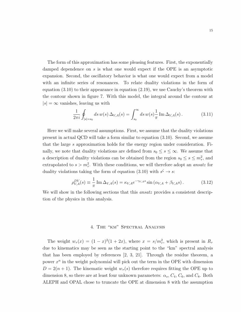
The form of this approximation has some pleasing features. First, the exponentially

damped dependence on s is what one would expect if the OPE is an asymptotic

expansion. Second, the oscillatory behavior is what one would expect from a model

with an infinite series of resonances. To relate duality violations in the form of

equation (3.10) to their appearance in equation (2.19), we use Cauchy’s theorem with

the contour shown in figure 7. With this model, the integral around the contour at

|s| =∞ vanishes, leaving us with

1

2πi

∮|s|=s0

dsw(s) ∆V,A(s) =

∫ ∞s0

dsw(s)1

πIm ∆V,A(s) . (3.11)

Here we will make several assumptions. First, we assume that the duality violations

present in actual QCD will take a form similar to equation (3.10). Second, we assume

that the large s approximation holds for the energy region under consideration. Fi-

nally, we note that duality violations are defined from s0 ≤ s ≤ ∞. We assume that

a description of duality violations can be obtained from the region s0 ≤ s ≤ m2τ , and

extrapolated to s > m2τ . With these conditions, we will therefore adopt an ansatz for

duality violations taking the form of equation (3.10) with sζ → s:

ρDVV,A(s) ≡ 1

πIm ∆V,A(s) = κV,Ae

−γV,As sin (αV,A + βV,As) . (3.12)

We will show in the following sections that this ansatz provides a consistent descrip-

tion of the physics in this analysis.

4. The “km” Spectral Analysis

The weight wτ (x) = (1 − x)2(1 + 2x), where x = s/m2τ , which is present in Rτ

due to kinematics may be seen as the starting point to the “km” spectral analysis

that has been employed by references [2, 3, 21]. Through the residue theorem, a

power xn in the weight polynomial will pick out the term in the OPE with dimension

D = 2(n + 1). The kinematic weight wτ (s) therefore requires fitting the OPE up to

dimension 8, so there are at least four unknown parameters: αs, C4, C6, and C8. Both

ALEPH and OPAL chose to truncate the OPE at dimension 8 with the assumption

16

that contributions from higher order terms were negligible. Additionally, both groups

made the assumption ∆V,A(s) = 0.

To create a data set large enough to fit four parameters, fits to the spectral function

data using the relation∫ s0

0

dswkm(s) ρV,A(s) = − 1

2πi

∮|s|=s0

dswkm(s) ΠOPEV,A (s), (4.1)

for the set of weights wkm(x) = (1 − x)k xmwτ (x) were employed. The choice of

moments (km) = (00), (10), (11), (12), and (13) provided a five point data set with

which to fit these four parameters at s0 = m2τ , the highest energy allowable by τ decay.

The values of αs(m2τ ) quoted in equation (2.2) were extracted using this method of

analysis.

4.1. Systematic Errors. Several systematic errors are introduced in the above anal-

ysis. First, there are at least two ways to partially resum the perturbative contribution

to ΠOPEV,A (s), CIPT and FOPT (cf. section 2.2). While these two methods have been

the subject of a number of investigations [7, 8, 9, 13], we instead choose to focus on

the non-perturbative systematic errors. Although we do not attempt to reconcile the

two methods of resummation, we will report on the results of our analysis using both

CIPT and FOPT.

Second, through the application of the residue theorem, the term in the polynomial

w(x) of order xn picks out a contribution only from the D = 2(n + 1) term in the

OPE. In the sum rules employed in the “km” analysis, this means that contributions

from the OPE up to D = 16 should in principle be included in the case of w13(x).

However, as mentioned above, this analysis truncates the OPE at dimension 8 with

the assumption that higher dimension contributions are negligible. Because the OPE

is at best an asymptotic series, the validity of this assumption is far from obvious.

An analysis of the contributions from each order in the OPE by reference [5] not

only found that dimension D > 8 terms may be numerically significant in the above

sum rules, but also demonstrated that an analysis which was consistent between

the degree of the weight and the truncation of the OPE shifted the central value of

17

0.0 0.5 1.0 1.5 2.0 2.5 3.0

0.00

0.02

0.04

0.06

0.08

0.10

0.12

0.14

s HGeV2L

ΡVHsL

Figure 8. OPAL vector channel spectral data (black) versus pertur-bation theory (red). The red band shows the theory deviations due tothe error on αs from the OPAL results reported in equation (2.2). Thepresence of duality violations is evident.

αs beyond its previously reported error margin. This indicates that the systematic

error introduced by truncating the OPE was not correctly accounted for in the “km”

analysis. As discussed below, we will require consistent treatment of the OPE by

restricting our analysis to weights of degree n ≤ 3.

Third, all previous analyses were executed under the assumption that any con-

tribution from duality violations to the sum rules employed were negligible. This

corresponds to setting ∆V,A = 0 in equation (2.19), or κ = 0 in the ansatz (3.12).

Figure 8 demonstrates the presence of duality violations in the perturbative spectral

function. Although the doubly pinched weights wkm(s) suppress these duality viola-

tions, the overall impact on the extraction of αs is relatively unknown. In light of

the extremely small errors obtained this assumption clearly needs to be investigated

quantitatively. The studies of references [19, 20] have suggested that this assumption

is, in fact, not valid. It is therefore reasonable to suggest that any analysis of τ decay

requires a more thorough evaluation of the effects of duality violations.

18

1 50 123

1

50

123

1 50 123

1

50

123

1 20 40 60 80 94

1

20

40

60

80

94

1 20 40 60 80 94

1

20

40

60

80

94

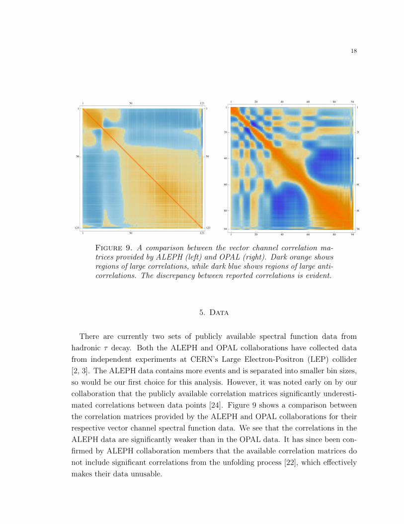
Figure 9. A comparison between the vector channel correlation ma-trices provided by ALEPH (left) and OPAL (right). Dark orange showsregions of large correlations, while dark blue shows regions of large anti-correlations. The discrepancy between reported correlations is evident.

5. Data

There are currently two sets of publicly available spectral function data from

hadronic τ decay. Both the ALEPH and OPAL collaborations have collected data

from independent experiments at CERN’s Large Electron-Positron (LEP) collider

[2, 3]. The ALEPH data contains more events and is separated into smaller bin sizes,

so would be our first choice for this analysis. However, it was noted early on by our

collaboration that the publicly available correlation matrices significantly underesti-

mated correlations between data points [24]. Figure 9 shows a comparison between

the correlation matrices provided by the ALEPH and OPAL collaborations for their

respective vector channel spectral function data. We see that the correlations in the

ALEPH data are significantly weaker than in the OPAL data. It has since been con-

firmed by ALEPH collaboration members that the available correlation matrices do

not include significant correlations from the unfolding process [22], which effectively

makes their data unusable.

19

The data we therefore use are the OPAL non-strange vector or axial-vector spec-

tral functions shown in figure 10. The spectral functions are binned in increments of

0.032 GeV2, up to smax = 3.120 GeV2 in the vector channel and smax = 3.088 GeV2

in the axial-vector channel. Correlation matrices between data points are provided

by OPAL, including cross-correlations between the vector and axial-vector data. Al-

though there have been recent improvements in the determination of constants present

in the normalization of this data, we do not expect these updates to significantly im-

pact results. We will therefore use the original OPAL normalizations in this analysis.

6. Fitting Strategies

The development of a more comprehensive fitting strategy begins with the require-

ment that the order of the OPE truncation be consistent with the weights employed

in the analysis. Restricting ourselves to weights of degree three or less provides us

with no more than four linearly independent weights. Even without the duality vio-

lation ansatz, this requires fitting four parameters: αs, C4, C6, and C8. To progress,

we must generate data by examining FESRs for a range of s0 values below m2τ . The

complete expression relating the non-strange experimental spectral function data to

theory is∫ s0

0

dsw(s) ρexpV,A(s) = − 1

2πi

∮|s|=s0

dsw(s) ΠOPEV,A (s)−

∫ ∞s0

dsw(s) ρDVV,A(s), (6.1)

with ΠOPEV,A (s) given by equation (2.18), ρDVV,A(s) given by equation (3.12), and ρexpV,A

the experimentally determined spectral functions.

Because the OPAL data is binned, the integral appearing on the left hand side of

equation (6.1) is replaced by a Riemann sum over all bins up to s0. Our data set is

generated by examining sum rules between smin ≤ s0 ≤ smax, where we always choose

smax = 3.120 GeV2 in the vector channel and smax = 3.088 GeV2 in the axial-vector

channel. Our data set in the vector channel is generated by the expression

dVi = (0.032 GeV2)

Ni∑j=1

w

(sj

sNi + 0.016 GeV2

)ρexpV (sj) , (6.2)

20

0.0 0.5 1.0 1.5 2.0 2.5 3.0

0.00

0.02

0.04

0.06

0.08

0.10

0.12

0.14

s HGeV2L

ΡVHsL

0.0 0.5 1.0 1.5 2.0 2.5 3.0

0.00

0.01

0.02

0.03

0.04

0.05

s HGeV2L

ΡAHsL

Figure 10. OPAL spectral functions. The top graph shows the vectorchannel data, while the bottom graph shows the axial-vector channeldata minus the pion peak.

21

where sj = j × 0.032 GeV2 for j = 1, 2, . . . , Ni, and Ni corresponds to the bin at

energy sNi for smin ≤ sNi ≤ smax. For the axial channel, the data does not include

the pion pole contribution (2.8) which is included in the expression on the right hand

side of (6.1). We add this contribution to the data, which gives us for the axial-vector

channel

dAi =

Ni∑j=1

[(0.032 GeV2)w

(sj

sNi + 0.016 GeV2

)ρexpA (sj) + 2f 2

π w

(M2

π

sNi + 0.016 GeV2

)],

(6.3)

where fπ = 0.0922 is the pion decay constant and Mπ = 0.140 GeV is the pion mass.

For a typical choice of smin = 1.5 GeV2, this provides roughly 50 data points per

moment with which to fit the theory expressions.

We choose to include terms in the OPE up to D = 8 in our analysis for several

reasons. First, we expect that the condensates are sensitive to duality violations.

Extracting their values from this analysis will therefore provide additional checks

on the impact of duality violations by comparing to previous determinations of the

condensates. The quality of existing data, however, makes it unlikely that we would

expect to obtain reliable estimates of condensates with D > 8. Moreover, although

little is known about the OPE, it is almost certainly not a convergent expansion and

so will break down at some order. It is therefore prudent to limit ourselves to a

relatively low maximum order in the OPE.

Because we assume the model presented in section 3 provides a reliable description

of the physics, we are no longer restricted to using moments that are at least doubly

pinched. Indeed, we find that to consistently fit the duality violation model at least

one unpinched moment should be included. This maximizes the contributions from

duality violations and helps determine the parameter values κV,A, γV,A, αV,A, and βV,A

in the ansatz (3.12). Here we will examine the set of weights

w0(x) = 1 ,

w2(x) = 1− x2 ,

w3(x) = (1− x)2(1 + 2x) , (6.4)

22

where x = s/s0. The weight w0 is unpinched, while the weights w2,3(x), which have

zeros at s = s0, are singly and doubly pinched respectively. These weights provide

a relatively smooth transition between emphasizing contributions from either duality

violations or the OPE, and will allow us to analyze the effect of our choice of moments

on this analysis.

Studies of higher orders in perturbation theory along the lines of references [8, 12]

appear to indicate that perturbation theory may be less convergent for sum rules

employing weights which include terms linear in x. For this reason we examine only

polynomials that do not include linear terms. A more detailed discussion of this

phenomenon will be found in a forthcoming publication [23].

6.1. Correlated Fits. Although the data generated by the methods described above

are highly correlated, it is possible to perform fully correlated fits to some moments.

This provides the simplest and most straight forward method of analysis. The func-

tion we wish to minimize is the standard χ2 function

χ2 = [di(n)− ti(n; ~p)]C−1ij [dj(n)− tj(n; ~p)], (6.5)

where di(n) and ti(n; ~p) represent the left and right hand sides of equation (6.1)

respectively for the choice of weight wn(x), Cij represents the complete integrated

covariance matrix for the data di(n), and a sum over repeated indices is implied. The

fit parameters contained in the expressions on the right hand side of equation (6.1)

are denoted by ~p. By definition we take i = 1 to be the label corresponding to the

data point where s0 = smin and imax to be the label corresponding to the data point

where s0 = smax.

The primary goal of this paper is to extract a value of αs(mτ ) with the lowest

possible fit error. The weight w0(x) = 1 represents the cleanest extraction method

for several reasons. Because w0(x) is independent of energy it weighs the entire

spectral function evenly. Additionally, w0(x) is unpinched, so it does not suppress

contributions from the duality violation ansatz which represents a large fraction of

the total number of parameters. The weight w2(x) also provides a stable fit and the

results are in excellent agreement with the results from w0(x). Conversely, fits only

23

to moments that are doubly pinched such as w3(x) do not produce stable fit results,

presumably due to their strong suppression of duality violations relative to the OPE.

We present results to fits using w0(x) in section 7.1.

We have also considered fits directly to the spectral function. This fit can be

cast in terms of a FESR by choosing the weight w(s) = δ(s− s0). The perturbative

expression for the spectral function can then be compared directly to the OPAL data.

However, these fits turn out to be less than ideal for multiple reasons. First, because

perturbation theory is only valid for sufficiently large energy, we are forced to exclude

a large section of data that the weighted integral in equation (6.1) can access. Second,

these fits are apparently not sensitive enough to αs which makes the fits unstable.

6.2. Diagonal Fits. It is of course interesting to examine simultaneous fits to mul-

tiple moments. Sum rules for multiple moments provide additional constraints on

the value of αs(m2τ ), so one might imagine the error on such a determination to be

reduced through this method. However, because the moments are not independent

of each other, the correlations between moments must be taken into account. These

cross-correlations end up being rather large, which lead to correlation matrices with

essentially zero eigenvalues at machine precision. In order to carry out an analysis of

multiple moments, we must therefore define non-standard “fit quality” functions Q2

which remove this obstacle.

The simplest thing to do in this case is to employ diagonal fits where all off-diagonal

elements of the integrated correlation matrix are omitted from the fit quality. The

new function we wish to minimize would then be given by

Q2diag =

∑n

imax∑i=1

[di(n)− ti(n, ~p)

ei(n)

]2, (6.6)

where ei(n) are the diagonal errors on di(n) and the sum over n represents a sum over

all weights wn(x) employed in the fit. This fixes the poor behavior of the correlation

matrix, but this fit quality no longer indicates the confidence level of the fit. Of course,

if Q2diag were to be interpreted as a traditional χ2 function, the errors produced by

such a fit would be significantly underestimated.

24

To account for the removal of all off-diagonal correlations in the fit quality Q2diag,

errors can be computed using the method detailed in appendix A. Errors can then

be computed for fit parameters including the full correlations between data using the

covariance matrix given by

〈δpi δpj〉 = A−1ik A−1jm

∂tn(~p)

∂pk

∂tq(~p)

∂pmC−1nl C

−1qr Clr , Aij ≡

∂tk(~p)

∂piC−1km

∂tm(~p)

∂pj. (6.7)

Here, C is the full integrated covariance matrix, including correlations between mo-

ments, and C is the integrated covariance matrix with all off-diagonal elements set

to zero. When possible, errors calculated with equation (6.7) have been compared to

standard χ2 errors, and have always been in good agreement. This lends confidence

to the propagation of errors in this fashion.

The results from such fits are found to be consistent with those obtained from the

strategy presented in section 6.1. However, due to the exclusion of all correlations in

the fits, errors on αs become much larger for fits to multiple moments. Because of

this we are led to consider other strategies that may help in reducing the fit error on

αs.

6.3. Other Strategies. The use of equation (6.7) makes it possible to explore fits

using other non-standard functions. It does not matter what fit qualityQ2 one chooses

to minimize as long as the errors are propagated correctly. Here we present a third

type of fit in which the full correlations for each moment are included, but the cross-

correlations between moments are not included in the fit. The function to minimize

is then

Q2block =

∑n

[di(n)− ti(n, ~p)]C−1ij (n) [dj(n)− tj(n, ~p)], (6.8)

where C(n) is the complete integrated covariance matrix for the weight wn(x). This

also solves the problem of having machine precision zero eigenvalues, but without

modifying the correlation matrix as severely as in section 6.2. Again, although it is

not possible to obtain an estimate of the confidence level of the fit from this function,

we may use the results to compare between the quality of fits performed using the

same method.

25

We wish to explore fits of this kind for the following reason. Suppose we consider

fits to two different moments with weights w and w′. The full covariance matrix then

has the form (Cw C

CT Cw′

),

where C is a matrix containing the cross-correlations between moments. In the case of

the weights presented in equation (6.4), however, the weights are nearly equal over a

significant range of s. This could conceivably lead to a situation where Cw ≈ Cw′ ≈ C,

which would then lead to a covariance matrix of the form(Cw Cw

Cw Cw

).

However, if we were to consider fitting to the same moment with weight w twice, one

would instead wish to use a correlation matrix of the form(Cw 0

0 Cw

),

with the fit quality function rescaled by a factor of 1/2.

Suspecting that our moments are closer to the latter case leads to this form of anal-

ysis. The errors on fit parameters would again be calculated by equation (6.7), with

C now being the block-diagonal covariance matrix and C being the full covariance

matrix including correlations between moments. Fits using this strategy lead to our

most precise determination of αs and are presented in section 7.2. Finally, it should

be noted that although we have explored a great many fitting strategies, it remains

an open question whether fit qualities different than equations (6.6) or (6.8) may lead

to a more precise determination of αs(m2τ ).

7. Fits

Here we present the results of fits performed as a function of smin. In section 7.1,

we explore fully correlated fits with the weight w0(x) = 1. As was discussed in section

6.1, results from correlated fits to both unpinched and singly-pinched moments were

not only in excellent agreement with each other, but also similarly stable as a function

26

of smin. Because of this, w0(x) is chosen to explore the differences between fits to the

vector channel, fits to the axial channel, and fits to both vector and axial channels.

We then use this information to obtain benchmark results for both FOPT and CIPT.

In section 7.2 we explore the inclusion of additional moments with the hope that

the added information will reduce the errors from single moment fits. However, as

discussed in section 6.2, fully correlated fits to multiple moments are not possible.

Instead, we utilize the fit quality functions (6.6) and (6.8) and obtain errors including

the full correlations from equation (6.7). These fits provide additional tests on the

ability of the duality violation model, equation (3.12), to describe the data, and

ultimately lead to a marginal improvement in the precision determination of αs.

In section 7.3 we examine fits which exclude the duality violation ansatz. We find

that even for doubly pinched weights such as w3(s) the results depend strongly on

the value of smin. We conclude that while varying s0 is necessary in order to impose

a consistent treatment of the OPE, it is not possible to do so without addressing the

presence of duality violations. As there is currently no systematic theory of duality

violations, this makes the inclusion of a model such as that represented by equation

(3.12) a necessity.

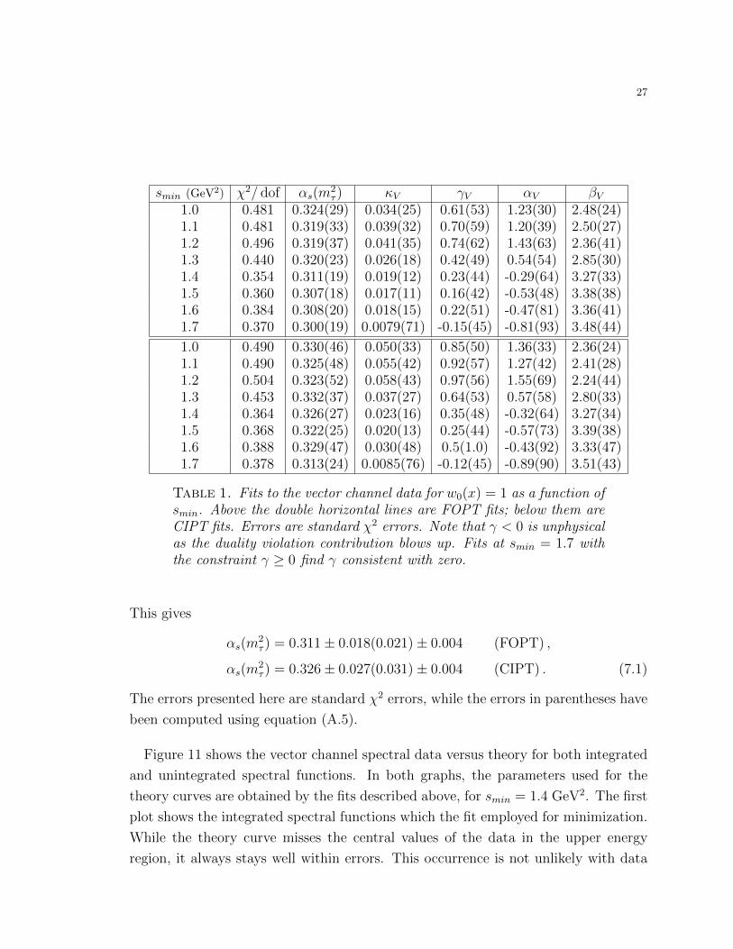
7.1. Fits to w0(x). Fully correlated fits using fit quality (6.5) are possible for fits

to w0(x) = 1. Table 1 presents the results of these fits to the OPAL vector channel

data including the χ2 value per degree of freedom as well as all values for the fit

parameters. Here the OPE coefficients appear only to non-leading order in αs, and

therefore have been neglected. We see that the fits are consistent for both CIPT and

FOPT across a wide range of smin values.

The χ2 per degree of freedom reaches a minimum at smin = 1.4 GeV2. For values

of smin ≥ 1.6 GeV2, however, the error on αs is larger. We will take our “benchmark”

results to be the fit results in the vector channel at smin = 1.4 GeV2. Because the χ2

per degree of freedom is essentially consistent between smin = 1.4 and 1.5 GeV2, we

will also allow for an error of ±0.004 from the variation in αs between these two fits.

27

smin (GeV2) χ2/ dof αs(m2τ ) κV γV αV βV

1.0 0.481 0.324(29) 0.034(25) 0.61(53) 1.23(30) 2.48(24)1.1 0.481 0.319(33) 0.039(32) 0.70(59) 1.20(39) 2.50(27)1.2 0.496 0.319(37) 0.041(35) 0.74(62) 1.43(63) 2.36(41)1.3 0.440 0.320(23) 0.026(18) 0.42(49) 0.54(54) 2.85(30)1.4 0.354 0.311(19) 0.019(12) 0.23(44) -0.29(64) 3.27(33)1.5 0.360 0.307(18) 0.017(11) 0.16(42) -0.53(48) 3.38(38)1.6 0.384 0.308(20) 0.018(15) 0.22(51) -0.47(81) 3.36(41)1.7 0.370 0.300(19) 0.0079(71) -0.15(45) -0.81(93) 3.48(44)

1.0 0.490 0.330(46) 0.050(33) 0.85(50) 1.36(33) 2.36(24)1.1 0.490 0.325(48) 0.055(42) 0.92(57) 1.27(42) 2.41(28)1.2 0.504 0.323(52) 0.058(43) 0.97(56) 1.55(69) 2.24(44)1.3 0.453 0.332(37) 0.037(27) 0.64(53) 0.57(58) 2.80(33)1.4 0.364 0.326(27) 0.023(16) 0.35(48) -0.32(64) 3.27(34)1.5 0.368 0.322(25) 0.020(13) 0.25(44) -0.57(73) 3.39(38)1.6 0.388 0.329(47) 0.030(48) 0.5(1.0) -0.43(92) 3.33(47)1.7 0.378 0.313(24) 0.0085(76) -0.12(45) -0.89(90) 3.51(43)

Table 1. Fits to the vector channel data for w0(x) = 1 as a function ofsmin. Above the double horizontal lines are FOPT fits; below them areCIPT fits. Errors are standard χ2 errors. Note that γ < 0 is unphysicalas the duality violation contribution blows up. Fits at smin = 1.7 withthe constraint γ ≥ 0 find γ consistent with zero.

This gives

αs(m2τ ) = 0.311± 0.018(0.021)± 0.004 (FOPT) ,

αs(m2τ ) = 0.326± 0.027(0.031)± 0.004 (CIPT) . (7.1)

The errors presented here are standard χ2 errors, while the errors in parentheses have

been computed using equation (A.5).

Figure 11 shows the vector channel spectral data versus theory for both integrated

and unintegrated spectral functions. In both graphs, the parameters used for the

theory curves are obtained by the fits described above, for smin = 1.4 GeV2. The first

plot shows the integrated spectral functions which the fit employed for minimization.

While the theory curve misses the central values of the data in the upper energy

region, it always stays well within errors. This occurrence is not unlikely with data

28

1.5 2.0 2.5 3.0

3.2

3.3

3.4

3.5

3.6

3.7

3.8

s0 HGeV2L

Rw

0Hs

0L

0.0 0.5 1.0 1.5 2.0 2.5 3.0

0.00

0.02

0.04

0.06

0.08

0.10

0.12

0.14

s HGeV2L

ΡVHsL

Figure 11. OPAL vector channel spectral function data (black dots)versus theory, with parameters from a fit to w0(x) at smin = 1.4 GeV2.The red curves are FOPT and the blue curves are CIPT. The top graphshows the integrated data as compared to Rw0(s0), normalized by a fac-tor of 12π2/s0. The bottom graph compares the OPAL spectral functiondirectly to perturbation theory + duality violations.

29

smin (GeV2) χ2/dof αs(m2τ ) κA γA αA βA

1.0 0.477 0.299(17) 0.063(31) 0.91(32) -0.58(31) -2.96(22)1.1 0.469 0.296(25) 0.058(39) 0.85(44) -0.69(68) -2.90(40)1.2 0.484 0.281(51) 0.045(36) 0.69(54) -1.2(1.3) -2.64(74)1.3 0.477 0.24(20) 0.035(19) 0.46(50) -2.0(2.1) -2.2(1.2)1.4 0.455 0.20(33) 0.041(20) 0.50(26) -2.49(36) -1.93(19)

1.0 0.482 0.315(22) 0.060(29) 0.89(32) -0.50(34) -3.01(23)1.1 0.472 0.309(33) 0.052(34) 0.79(43) -0.70(77) -2.90(45)1.2 0.485 0.284(78) 0.0400(31) 0.61(56) -1.3(1.6) -2.56(89)1.3 0.477 0.23(21) 0.034(14) 0.44(37) -2.1(1.7) -2.11(92)1.4 0.455 0.20(33) 0.041(30) 0.50(26) -2.50(36) -1.93(19)

Table 2. Fits to the axial channel data for w0(x) = 1 as a functionof smin. Above the double horizontal lines are FOPT fits; below themare CIPT fits. Errors are standard χ2 errors. Note that the constraintαs(mτ ) ≥ 0.20 has been enforced, such that the fits with smin = 1.4GeV2 have reached that limit.

that is as highly correlated as ours. The second graph shows the unintegrated spectral

functions, demonstrating that the duality violation ansatz (3.12) is indeed a reliable

description of the data.

As can be seen in table 2, fits to the axial-vector channel alone are not as consistent

as in the vector channel. This is primarily attributed to the fact that the only major

feature present in the axial channel is the a1 resonance, which has a wide width

and peaks at ∼ 1.3 GeV2. In order to successfully fit the duality violation ansatz,

features attributed to duality violations must be present in the range smin ≤ s ≤ smax.

Bearing in mind that equation (3.12) is an asymptotic solution for duality violations,

it is possible that our model has not set in at such low energies in the axial channel.

We can of course also perform combined fits to both the vector and axial channels

using fit quality (6.5) in the hope that the added information will further constrain

αs(m2τ ) and reduce the fit error. However, although the fit results appear consistent

with vector channel fits, the fit quality becomes very flat in parameter space which

leads to both physical and unphysical solutions. Fits employing fit quality (6.6) do

not appear to have this problem but, as discussed in section 6.2, the errors on αs

30

smin (GeV2) Q2diag/dof αs(m

2τ ) κV,A γV,A αV,A βV,A

1.3 1.96/106 0.301(25) 0.037(54) 0.64(97) -0.8(1.6) 3.58(89)0.064(58) 0.86(55) -0.6(1.6) -2.95(86)

1.4 1.84/100 0.299(29) 0.032(51) 0.6(1.0) -1.0(2.1) 3.7(1.1)0.068(96) 0.89(77) -0.7(1.8) -2.90(96)

1.5 1.79/94 0.299(33) 0.029(52) 0.5(1.1) -1.0(2.5) 3.7(1.3)0.06(13) 0.8(1.1) -0.7(1.9) -2.9(1.0)

1.6 1.60/88 0.300(39) 0.026(60) 0.5(1.3) -0.9(2.8) 3.6(1.4)0.04(14) 0.7(1.5) -0.8(1.9) -2.83(97)

1.3 2.03/106 0.315(33) 0.043(63) 0.71(98) -0.8(1.6) 3.60(90)0.059(55) 0.81(55) -0.6(1.6) -2.94(86)

1.4 1.89/100 0.313(37) 0.037(58) 0.6(1.0) -1.1(2.1) 3.7(1.1)0.063(91) 0.84(79) -0.7(1.8) -2.89(94)

1.5 1.83/94 0.312(42) 0.033(58) 0.6(1.1) -1.1(2.5) 3.7(1.3)0.06(12) 0.08(1.1) -0.8(1.9) -2.87(97)

1.6 1.62/88 0.313(51) 0.029(65) 0.5(1.2) -1.0(3.0) 3.7(1.5)0.04(13) 0.6(1.6) -0.9(1.7) -2.82(92)

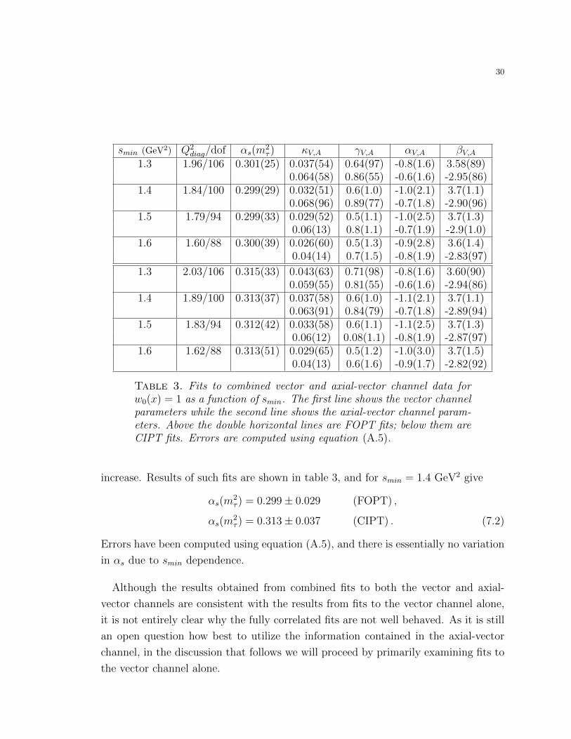
Table 3. Fits to combined vector and axial-vector channel data forw0(x) = 1 as a function of smin. The first line shows the vector channelparameters while the second line shows the axial-vector channel param-eters. Above the double horizontal lines are FOPT fits; below them areCIPT fits. Errors are computed using equation (A.5).

increase. Results of such fits are shown in table 3, and for smin = 1.4 GeV2 give

αs(m2τ ) = 0.299± 0.029 (FOPT) ,

αs(m2τ ) = 0.313± 0.037 (CIPT) . (7.2)

Errors have been computed using equation (A.5), and there is essentially no variation

in αs due to smin dependence.

Although the results obtained from combined fits to both the vector and axial-

vector channels are consistent with the results from fits to the vector channel alone,

it is not entirely clear why the fully correlated fits are not well behaved. As it is still

an open question how best to utilize the information contained in the axial-vector

channel, in the discussion that follows we will proceed by primarily examining fits to

the vector channel alone.

31

smin Q2diag αs(m

2τ ) κV γV αV βV C6,V C8,V

(GeV2) dof1.3 6.00/167 0.299(27) 0.035(63) 0.6(1.1) -1.3(1.7) 3.83(95) -0.0059(51) 0.0094(83)1.4 4.28/158 0.298(28) 0.025(42) 0.5(1.1) -1.4(2.1) 3.9(1.1) -0.0062(51) 0.0102(83)1.5 3.20/149 0.297(28) 0.019(29) 0.31(99) -1.4(2.3) 3.9(1.2) -0.0065(50) 0.0109(82)1.6 2.04/137 0.294(24) 0.009(15) 0.00(97) -1.2(22) 3.8(1.1) -0.0075(39) 0.0131(63)

1.3 0.186/167 0.323(53) 0.039(58) 0.7(1.0) -0.4(2.1) 3.4(1.1) -0.0048(73) 0.006(13)1.4 0.173/158 0.322(58) 0.039(53) 0.65(95) -0.4(2.6) 3.4(1.3) -0.0049(83) 0.007(15)1.5 0.136/149 0.326(71) 0.047(65) 0.73(93) -0.2(3.1) 3.3(1.6) -0.004(11) 0.005(21)1.6 0.0933/137 0.333(95) 0.07(15) 0.9(1.1) 0.1(3.8) 3.1(2.0) -0.0026(17) 0.001(37)

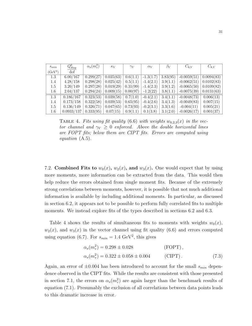
Table 4. Fits using fit quality (6.6) with weights w0,2,3(x) in the vec-tor channel and γV ≥ 0 enforced. Above the double horizontal linesare FOPT fits; below them are CIPT fits. Errors are computed usingequation (A.5).

7.2. Combined Fits to w0(x), w2(x), and w3(x). One would expect that by using

more moments, more information can be extracted from the data. This would then

help reduce the errors obtained from single moment fits. Because of the extremely

strong correlations between moments, however, it is possible that not much additional

information is available by including additional moments. In particular, as discussed

in section 6.2, it appears not to be possible to perform fully correlated fits to multiple

moments. We instead explore fits of the types described in sections 6.2 and 6.3.

Table 4 shows the results of simultaneous fits to moments with weights w0(x),

w2(x), and w3(x) in the vector channel using fit quality (6.6) and errors computed

using equation (6.7). For smin = 1.4 GeV2, this gives

αs(m2τ ) = 0.298± 0.028 (FOPT) ,

αs(m2τ ) = 0.322± 0.058± 0.004 (CIPT) . (7.3)

Again, an error of ±0.004 has been introduced to account for the small smin depen-

dence observed in the CIPT fits. While the results are consistent with those presented

in section 7.1, the errors on αs(m2τ ) are again larger than the benchmark results of

equation (7.1). Presumably the exclusion of all correlations between data points leads

to this dramatic increase in error.

32

smin Q2block αs(m

2τ ) κV γV αV βV C6,V C8,V

(GeV2) dof1.3 0.415 0.300(18) 0.050(35) 0.87(48) 0.38(77) 2.87(44) -0.0039(40) 0.0045(62)1.4 0.329 0.304(17) 0.027(18) 0.46(88) -0.48(88) 3.35(48) -0.0043(31) 0.0067(47)1.5 0.326 0.304(19) 0.021(12) 0.31(38) -0.7(1.1) 3.46(58) -0.0046(33) 0.0076(51)1.6 0.338 0.305(25) 0.029(23) 0.48(48) -0.5(1.6) 3.39(81) -0.0043(51) 0.0067(87)1.7 0.329 0.300(26) 0.010(77) 0.00(39) -0.9(1.6) 3.53(81) -0.0060(46) 0.0106(74)

1.3 0.399 0.332(47) 0.035(32) 0.60(64) 0.5(1.0) 2.84(52) -0.0027(59) 0.0019(95)1.4 0.319 0.326(31) 0.023(16) 0.34(47) -0.3(1.0) 3.27(54) -0.0044(36) 0.0059(58)1.5 0.320 0.322(31) 0.019(13) 0.26(42) -0.6(1.3) 3.39(66) -0.0050(37) 0.0073(62)1.6 0.333 0.323(46) 0.027(21) 0.43(50) -0.4(1.9) 3.33(98) -0.0047(62) 0.006(11)1.7 0.327 0.314(37) 0.011(79) 0.00(40) -0.9(1.8) 3.50(88) -0.0067(46) 0.0109(81)

Table 5. Fits using fit quality (6.8) with weights w0,2,3(x) in the vec-tor channel and γV ≥ 0 enforced. Above the double horizontal linesare FOPT fits; below them are CIPT fits. Errors are computed usingequation (A.5).

Motivated by the discussion in section 6.3, we can also perform fits to the block

diagonal fit quality (6.8), where correlations within each moment are kept but ignoring

correlations between moments. The results of these fits are shown in table 5, and for

smin = 1.4 GeV2 yields

αs(m2τ ) = 0.304± 0.017 (FOPT) ,

αs(m2τ ) = 0.326± 0.031± 0.004 (CIPT) . (7.4)

Errors have again been computed using equation (6.7), while an error of ±0.004 has

been added to the CIPT result to account for the variation in the central value of

αs from neighboring fits with essentially the same fit quality. The fit results are in

excellent agreement with those presented in section 7.1, while we find a marginal

improvement in the error on αs(m2τ ).

Figure 12 shows the FOPT results from equation (7.4) plotted versus Rτ (s0). This

fit incorporated each of the weights in equation (6.4) and we find that the theory

expressions are able to describe the integrated data sets within error for each of these

weights. It appears that the duality violation ansatz is even able to describe moments

that are doubly pinched, further verifying the ability of equation (3.12) to correctly

33

1.5 2.0 2.5 3.0

1.80

1.85

1.90

1.95

2.00

2.05

2.10

s0 HGeV2L

Rw

3Hs

0L

Figure 12. Integrated OPAL vector channel spectral function data(black dots) versus theory, with parameters from a combined fit tow0,2,3(s) at smin = 1.4 GeV2. The red curve is FOPT and the bluecurve is FOPT. The integrated data has been normalized by a factor of12π2/s0.

describe the physics. Indeed, the consistency between the values of αs(m2τ ) obtained

across a variety of moments provides strong support for our model.

Although our primary concern in this section has been a study of vector channel

fits, we have also explored fits employing multiple weight functions to both the vector

and axial-vector channels. However, inclusion of the axial-vector channel data again

leads to additional complications. In particular, block diagonal fits using fit quality

(6.8) are no longer stable, and we must resort to diagonal fits using fit quality (6.6).

Results for FOPT fits are presented in table 6, and for smin = 1.4 GeV2 this fit yields

αs(m2τ ) = 0.292± 0.022 (FOPT) . (7.5)

Errors have been computed using equation (6.7), and there is essentially no variation

in αs(m2τ ) due to a dependence on smin.

34

smin Q2diag αs(m

2τ ) κV,A γV,A αV,A βV,A C6,(V,A) C8,(V,A)

(GeV2) dof1.3 13.4/332 0.293(21) 0.043(79) 0.7(1.2) -1.8(1.7) 4.10(93) -0.0069(40) 0.0112(64)

0.068(71) 0.86(61) -1.0(1.4) -2.72(76) -0.0001(40) 0.0050(69)1.4 9.94/314 0.292(22) 0.025(44) 0.4(1.1) -2.0(2.1) 4.2(1.1) -0.0073(40) 0.0121(74)

0.08(12) 0.92(84) -1.1(1.5) -2.71(80) -0.0005(40) 0.0062(68)1.5 7.63/296 0.291(22) 0.013(22) 0.2(1.0) -2.0(2.3) 4.2(1.2) -0.0077(38) 0.0132(82)

0.08(17) 0.9(1.1) -1.1(1.5) -2.68(76) -0.0009(38) 0.0068(63)1.6 5.14/272 0.291(20) 0.009(18) 0.0(1.1) -1.6(2.3) 3.9(1.2) -0.0081(33) 0.0141(90)

0.05(17) 0.8(1.5) -1.2(1.1) -2.62(57) 0.0004(33) 0.0047(54)

Table 6. Fits to the combined vector and axial-vector channels usingfit quality (6.6) with weights w0,2,3(x). The first line shows the vectorchannel parameters, while the second line shows the axial-vector pa-rameters. FOPT results are shown, with γV ≥ 0 enforced. Errors arecomputed using equation (A.5).

7.3. Fits Excluding Duality Violations. The values of αs reported here are clearly

different than those found in references [2, 3], with larger errors. One might then

wonder how much of this shift is due to our more consistent treatment of the OPE,

and how much is due to the inclusion of our duality violation ansatz. However, it turns

out that these systematics are not so easy to disentangle. As was already explained

in section 6, consistency between the OPE truncation and the degree of the weight

w(s) necessitates varying s0 below m2τ . As we will show, the exclusion of our duality

violation model then makes the fits much more sensitive to the choice of smin, which

implies a significant effect from duality violations.

To perform fits that exclude duality violations, in other words to assume that

ρV,ADV (s)→ 0 in equation (6.1), we must restrict ourselves to weights that are at least

doubly pinched. The only weight that satisfies this criteria with degree ≤ 3 that

does not include a term linear in s is the kinematic weight w3(s). Table 7 shows the

results of a fit to the vector channel using fit quality (6.5) with no model for duality

violations included.

Because the fits do not require fitting the duality violation ansatz (3.12), we are

able to scan a larger range of smin. However, it is clear that the results here depend

much more strongly on smin than the results presented in previous sections which

35

smin (GeV2) χ2/dof αs(m2τ ) C6,V C8,V

1.3 2.44 0.3868(14) 0.000221(35) 0.01313(74)1.4 2.52 0.3897(21) 0.00235(37) 0.01399(90)1.5 2.65 0.3893(55) 0.00235(43) 0.0139(17)1.6 2.02 0.322(13) 0.00666(86) 0.01390(88)1.7 0.92 0.298(13) 0.00958(80) 0.0182(10)1.8 0.54 0.278(16) 0.0120(10) 0.0222(15)1.9 0.33 0.260(16) 0.0144(13) 0.0267(21)2.0 0.34 0.260(19) 0.0145(18) 0.0268(32)2.1 0.35 0.260(22) 0.0143(25) 0.0263(47)2.2 0.34 0.270(21) 0.0125(27) 0.0222(55)2.3 0.37 0.272(16) 0.0121(21) 0.0213(45)

Table 7. Correlated fits using fit quality (6.5) with w3(s) in the vectorchannel. FOPT results are shown, and no model for duality violationsis included (ρVDV (s)→ 0).

include the ansatz. The value of αs stabilizes at smin ≥ 1.9 GeV2, but the χ2 value

per degree of freedom would lead us to pick a value of αs(m2τ ) ≈ 0.26± 0.02 which is

very different from the values obtained in the previous sections. Fits including both

the vector and axial-vector data suffer from similar inconsistencies, and would lead

to a value of αs(m2τ ) ≈ 0.29 ± 0.02, which is barely consistent with the result from

the vector channel only.

8. Summary of Results

The results presented in the previous sections demonstrate that fit results including

the ansatz (3.12) are stable not only as a function of smin, but also between different

fitting strategies and choice of weights. Because of this consistency, we choose to

present the results from fits with the smallest fit errors for our preliminary value of

αs(m2τ ). This was found by using the block diagonal fit quality (6.8) with weights

w0(s), w2(s), and w3(s) in the vector channel. These results were presented in table

36

5, and for smin = 1.4 GeV2 we find

αs(m2τ ) = 0.304± 0.017 (FOPT) ,

αs(m2τ ) = 0.326± 0.031 (CIPT) . (8.1)

The fit errors have been computed using equation (6.7), and the CIPT errors have

been added in quadrature.

Comparing these results with the original results of equation (2.2) from the OPAL

and ALEPH collaborations, we find both a significant shift in the central values and

an increase in the fit errors. In order to compare these results with the 2009 world

average, these values must be scaled to the Z mass. This gives us

αs(M2Z) = 0.1166± 0.0023 (FOPT) ,

αs(M2Z) = 0.1193± 0.0038 (CIPT) . (8.2)

The errors have been computed by averaging the slightly asymmetrical results which

arise when scaling the values at ± 1σ. We find that our results have shifted beyond

the previously reported errors from OPAL data analysis which, at the Z mass, gave

αs(M2Z) = 0.1219 ± 0.0010exp ± 0.0017th using CIPT. Comparing to the value cited

in equation (2.1), we find that our new results are certainly in better agreement than

this previous incomplete estimate.

These are results to fits of the unmodified OPAL vector channel spectral function

data. The errors quoted are fit errors only, and do not yet account for all possible

sources of error. In particular, we have not attempted to estimate the error due to

the truncation of the perturbative series. Additionally, we have not included the

information contained in the axial-vector spectral function data, as fits including

this data are not yet fully understood. The instability in the fits to only the axial-

vector channel raises concerns regarding the ability of the duality violation ansatz to

accurately describe the physics present in the axial-vector channel. It is left to future

studies to determine how best to incorporate the axial-vector information into our

current strategy.

37

9. Conclusion

Here we have presented an updated framework for the analysis of hadronic τ decay

data including a comprehensive treatment of systematic errors which were previously

unaccounted for. Following the work of reference [5], we have required that the

truncation of the OPE be consistent with the highest degree of weights employed.

This requirement then necessitates employing sum rules below s0 = m2τ . As we

demonstrated in section 7.3, this in turn required a quantitative study of duality

violations. By introducing a physically motivated ansatz to account for duality vio-

lations, we were then able to determine the value of αs(m2τ ) from hadronic τ decay

including quantitative estimates of these systematic errors which had not previously

been quantitatively investigated.

The accuracy of the results presented here depends in part on our ability to correctly

model the physics present in duality violations. Conservatively, these results can be

seen as a lower bound on the error introduced by ignoring duality violations. However,

the stability of αs, a purely perturbative parameter, across the range of moments

analyzed here provides strong support for the validity of our ansatz. We conclude not

only that the ansatz is able to accurately describe the data but also that it provides

a reasonable estimate of the physics present in duality violations.

The inclusion of an ansatz for duality violations comes at the price of introducing

four new fit parameters per channel. Regardless, we have demonstrated that this

method of analysis is feasible. The presence of additional parameters, combined with

the necessity of examining sum rules below s0 = m2τ , lead to larger errors than have

previously been reported. Additionally, the central values from preliminary estimates

vary outside the error margin of the previous estimates using OPAL data. These

results demonstrate that the previous analyses are afflicted by uncertainties that can

not be ignored.

With the demonstration that previously errors have been significantly underesti-

mated, there is certainly room for improvement on the precision of αs obtained from

hadronic τ decay. We have presented a new framework for this analysis, but the next

step in precision improvement will likely be with the introduction of improved data.

38

With the comprehensive framework developed here along with the future improve-

ment in data quality, we expect that higher precision results can be reached.

Appendix A. Linear Fluctuation Analysis

We begin by defining a minimizing function as

Q2 = [di − ti(~p)] C−1ij [dj − tj(~p)], (A.1)

where di is the experimental data set, ti(~p) is a function that describes this data for

a set of parameters ~p, C is a positive-definite but otherwise arbitrary matrix, and a

sum over repeated indices is implied. In the case where C = C, this becomes the χ2

function for a fully correlated fit. The minimum of equation (A.1) is given by

∂Q2

∂pi= −2

∂tj(~p)

∂piC−1jk [dk − tk(~p)] = 0. (A.2)

We wish to determine how fluctuations in the experimental data, δdj, will affect

the values of the fit parameters ~p. To do so we take the derivative of equation (A.2)

with respect to both dl and pl. This gives(∂tj(~p)

∂piC−1jk

∂tk(~p)

∂pl− ∂2tj(~p)

∂pi ∂plC−1jk [dk − tk(~p)]

)δpl =

∂tj(~p)

∂piC−1jk δdk (A.3)

Provided that the difference dk − tk(~p) can be considered to be small, we may drop

the term proportional to the second derivative on the left hand side. We then obtain

an expression for the fluctuations in the fit parameters as a linear function of the data

fluctuations,

δpl = A−1li∂tj(~p)

∂piC−1jk δdk , where Ail ≡

∂tj(~p)

∂piC−1jk

∂tk(~p)

∂pl. (A.4)

Equation (A.4) can now be used to compute the covariance matrix for the fit

parameters in terms of the full covariance matrix of the experimental data:

〈δpi δpj〉 = A−1ik Ajl∂tm(~p)

∂pk

∂tn(~p)

∂plC−1mr C

−1ns 〈δdr δds〉 , (A.5)

39

where 〈δdr δds〉 = Crs is the full experimental covariance matrix. This provides an

estimate for the full covariance matrix of the parameter set ~p. In the particular case

in which C = C, this result simplifies to

〈δpiδpj〉 =

(∂tk(~p)

∂piC−1km

∂tm(~p)

∂pj

)−1, (A.6)

which is equal to the familar χ2 error matrix estimate assuming once again that

di − ti(~p) is small.

References

[1] E. Braaten, S. Narison and A. Pich, QCD analysis of the tau hadronic width, Nucl. Phys. B373 (1992) 581.

[2] S. Schael et al. [ALEPH Collaboration], Branching ratios and spectral functions of tau decays:Final ALEPH measurements and physics implications, Phys. Rept. 421 (2005) 191 [arXiv:hep-ex/0506072]

[3] K. Ackerstaff et al. [OPAL Collaboration], Measurement of the strong coupling constant alpha(s)and the vector and axial-vector spectral functions in hadronic tau decays, Eur. Phys. J. C 7, 571(1999) [arXiv:hep-ex/9808019]

[4] S. Bethke, The 2009 world average of αs, Eur. Phys. J. C 64 (2009) [arXiv:0908.1135][5] K. Maltman and T. Yavin, αs(MZ) from hadronic tau decays, Phys. Rev. D 78 (2008)

[arXiv:0807.0650][6] M. Davier et al., The determination of alpha(s) from tau decays revisited, Eur. Phys. J. C 56,

305 (2008) [arXiv:0803.0979]

[7] P.A. Baikov, K.G. Chetyrkin, and J.H. Kuhn, Hadronic Z- and tau- Decays in Order alpha s4,Phys. Rev. Lett. 101 (2008) [arXiv:0801.1821]

[8] M. Beneke and M. Jamin, alpha s and the tau Hadronic Width: Fixed-order, Contour Improvedand Higher-order Perturbation Theory, Martin Beneke, JHEP 0809 (2008) [arXiv:0806.3156]

[9] S. Menke, On the Determination of alpha s from Hadronic tau Decay with Contour-improved,Fixed Order and Renormalon-chain Perturbation Theory, [arXiv:0904.1796]

[10] S. Narison, Power Corrections to alpha s(M tau), —V {us}— and m s, Phys. Lett. B673, 30(2009) [arXiv:0901.3823]

[11] E. de Rafael, An Introduction to Sum Rules in QCD, (1998) [arXiv:hep-ph/9802448v1][12] M. Jamin, Contour-improved Versus Fixed Order Perturbation Theory in Hadronic τ Decay,

JHEP 0509 (2005) [arXiv:hep-ph/0509001v2][13] I. Caprini and J. Fisher, αs from τ Decays: Contour-Improved versus Fixed Order summation

in a New QCD Perturbation Expansion, Eur. Phys. J. C 64 (2009)[14] A. A. Pivovarov, Renormalization Group Analysis of the Tau-Lepton Decay within QCD, Z.

Phys. C 53 (2003)

40

[15] F. Le Diberder and A. Pich, The Perturbative QCD Prediction to R(tau) Revisited, Phys. Lett.B286 (1992)

[16] M. A. Shifman, Quark-Hadron Duality, [arXiv:hep-ph/0009131][17] B. Blok, M. A. Shifman, and D. X. Zhang, An Illustrative Example of How Quark-Hadron

Duality Might Work, Phys. Rev. D 57, 2691 (1998) [arXiv:9709333][18] I. I. Y. Bigi, M. A. Shifman, N. Uraltsev, and A. I. Vainshtein, Heavy Flavor Decays, OPE and

Duality in Two-Dimensional ’t Hooft Model, Phys. Rev. D 59 (1999) [arXiv:hep-ph/9805241][19] O. Cata, M. Golterman, and S. Peris, Unraveling duality violations in hadronic tau decays,

Phys. Rev. D 77 (2008) [arXiv:0803.0246][20] O. Cata, M. Golterman, and S. Peris, Possible duality violations in tau decay and their impact

on the determination of αs, Phys. Rev. D 79 (2008) [arXiv:0812.2285][21] F. Le Diberder and A. Pich, Testing QCD with tau Decays, Phys. Lett. B289 (1992)[22] M. Davier, A. Hocker, B. Malaescu, and Z. Zhang, private communication.[23] D. Boito, O. Cata, M. Golterman, M. Jamin, K. Maltman, J. Osborne, and S. Peris, In prepa-

ration.[24] D. Boito et al., Duality Violations in Tau Hadronic Spectral Moments, [arXiv:1011.4426v1]