ON LARGE RING SOLUTIONS FOR GIERER-MEINHARDT SYSTEM …jcwei/gm-largering-10-11-12.pdf · ON LARGE...

ON LARGE RING SOLUTIONS FOR GIERER-MEINHARDT

SYSTEM IN R3

T. KOLOKOLONIKOV, JUNCHENG WEI, AND WEN YANG

Abstract. We consider the stationary radial solution in the classical Gierer-Meinhardt system in R

3:

ǫ2∆u− u+ u2

v= 0 in R

3,

∆v − v + u2 = 0 in R3,

u, v > 0, u(x), v(x) → 0 as |x| → +∞.

We prove the existence of a large ring-like solution. This complements anearlier work of Ni and Wei [33] in which the existence of O(1) ring solutionswas proved in R

2.

1. introduction

Of concern is the stationary Gierer-Meinhardt system in R3:

ε2∆u− u+ u2

v= 0 in R

3,

∆v − v + u2 = 0 in R3,

u > 0, v > 0, u(x), v(x) → 0 as |x| → +∞,

(1.1)

where ε > 0 is a small constant.Gierer-Meinhardt system was proposed in [14] to model head formation of hydra,

an animal of a few millimeters in length, made up of approximately 100,000 cellsof about fifteen different types. It consists of a “head” region located at one endalong its length. Typical experiments with hydra involve removing part of the“head” region and transplanting it to other parts of the body column. Then, anew “head” will form if the transplanted area is sufficiently far from the (old)head. These observations led to the assumption of the existence of two chemicalsubstances—a slowly diffusing activator u and a rapidly diffusing inhibitor v. Theratio of their diffusion rates, denoted by ε, is assumed to be small.

The Gierer-Meinhardt system falls within the framework of a theory proposedby Turing [35] in 1952 as a mathematical model for the development of complexorganisms from a single cell. He speculated that localized peaks in concentrationof chemical substances, known as inducers or morphogens, could be responsiblefor a group of cells developing differently from the surrounding cells. Turing dis-covered through linear analysis that a large difference in relative size of diffusivi-ties for activating and inhibiting substances carries instability of the homogeneous,constant steady state, thus leading to the presence of nontrivial, possibly stablestationary configurations. Activator-inhibitor systems have been used extensivelyin the mathematical theory of biological pattern formation [21], [22]. Among themGierer-Meinhardt system has been the object of extensive mathematical treatment

1991 Mathematics Subject Classification. Primary 35J55, 35B25; Secondary 35J60, 92C37.Key words and phrases. Gierer-Meinhardt system, radial solution, singular perturbations.

1

2 T. KOLOKOLONIKOV, JUNCHENG WEI, AND WEN YANG

in recent years. We refer the reader to two survey articles [25, 42] for a descriptionof progress made and references.

In particular, it has been a matter of high interest to study nonconstant positivesteady states, namely, solutions of the following elliptic system

ε2∆u− u+ up

vq = 0 in Ω,

D∆v − v + um

vs = 0 in Ω,

∂u∂ν

= ∂v∂ν

= 0 on ∂Ω,

(1.2)

where the exponents (p, q,m, s) satisfy the following condition:

p > 1, q > 0,m > 1, s ≥ 0,qm

(p− 1)(1 + s)> 1. (1.3)

A first step in solving Problem (1.2) is to study its shadow system, namely, wetake D = +∞ first. By suitable scaling, the study of steady-state for the shadowsystem can be transformed to that of the scalar equation

ε2∆u− u+ up = 0 in Ω,

u > 0 in Ω, ∂u∂ν

= 0 on ∂Ω.(1.4)

For problem (1.4), there have been intense works on the construction of a singleor multiple spikes. For the case p in subcritical range, we refer the readers to thearticles [6], [7], [15], [16], [29], [36], [38] and the references therein, starting with thepioneering works [17], [26], [27], [28], [32]. For the critical exponent case, we referto the papers [3], [4], [13], [31], and the references therein. A review of the subjectup to 2004 can be found in [42].

In the case of finite D and bounded domain case, Takagi [34] first constructedmultiple symmetric peaks in the one-dimensional case. In higher dimensional case,Ni and Takagi [29] constructed multiple boundary spikes in the case of axiallysymmetric domains, assuming that D is large. Multiple interior spikes for finite Dcase in a bounded two dimensional domain are constructed in [39], [40] and [41].The stability of multiple spikes as well as the dynamics of spikes are considered in[11], [30], [37], [40], [41] and the references therein.

From now on, we focus on the case of Ω = RN . Problem (1.2) has been shown

to exhibit single or multiple bump solutions in one or two dimensions. See [8], [9],[11], [12] and the references therein.

A long-standing problem is the existence of radially symmetric bound states inR

N when N ≥ 3. (See also page 579 of [42].) Ni and Wei [33] first constructedring-like solutions for the generalized Gierer-Meinhardt system

ε2∆u− u+ up

vq = 0 in RN ,

∆v − v + um

vs = 0 in RN ,

u > 0, v > 0, u(x), v(x) → 0 as |x| → +∞,

(1.5)

where (p, q,m, s) satisfies, in addition to the usual structural condition (1.3), thefollowing new condition

(N − 2)q

N − 1+ 1 < p < q + 1 if N ≥ 3; 1 < p ≤ q + 1 if N = 2. (1.6)

These are radially symmetric solutions such that u concentrates on an the surfaceof a ball of a certain O(1) radius as ε→ 0. In the case of R2, the first two authorsshowed in [19] that there are solutions with multiple clustered rings.

ON LARGE RING SOLUTIONS FOR GIERER-MEINHARDT SYSTEM IN R3 3

In R3, unfortunately the classical Gierer-Meinhardt system (1.1) (i.e. p = 2, q =

1), lies at the bordeline case (p = q + 1) in the condition (1.6). The purpose ofthis paper is to give a confirmative answer to the existence of radially symmetricbound states of the classical Gierer-Meinhardt system (1.1) in R

3. This seems tobe the first radial bound states for Gierer-Meinhardt system. We should remarkthat as far as non-radial solutions are concerned, in [20], a smoke-ring solution wasconstructed for (1.5) with N = 3, provided that (p, q,m, s) satisfy

p = q + 1, 1 < m− s < 3. (1.7)

This includes the case of the classical GM system (1.1). A smoke-ring solutionconcentrates on a circle in R

3 and is axi-symmetric but not radially symmetric.Before we state the main result of this paper, we define some notations to be

used throughout the paper. Let the Green function be

G′′ +2

rG′ −G+ δ(r − r0) = 0, G′(0, r0) = 0. (1.8)

Its solution is given by

G(r, r0) =

r02r (e

r−r0 − e−r−r0) = r0re−r0 sinh(r), r < r0,

r02r (e

r0−r − e−r−r0) = r0re−r sinh(r0), r > r0.

(1.9)

Let w(y) be the unique solution for the following ODE:

w′′

− w + w2 = 0 in R, w > 0, w(0) = maxy∈R

w(y), w(y) → 0 as |y| → ∞; (1.10)

it is well known that

w(y) =3

2sech2

(y

2

)

.

We now state our main theorem in this paper.

Theorem 1.1. For ε sufficiently small, problem (1.1) has a solution with the fol-lowing properties:

• uε,R, vε,R are radially symmetric,• uε,R = 1

6εG(rε,rε)w(

r−rεε

)

(1 + o(1)),

• vε,R = 16εG(rε,rε)2

G(r, rε)(1 + o(1)), where rε stands for the solution of the

following equation

(2r + 1)e−2r =103

70ε. (1.11)

Asymptotically the radius rǫ behaves like

rǫ =1

2log

1

ǫ+O(log log

1

ǫ); (1.12)

so in fact rε → ∞ as ε→ 0. In contrast, for the general GM model (1.5) and underconditions (1.6), the ring radius was derived in [33]; it was found that when N = 3,rε → r0 where r0 satisfies

p− 1

q=e2r0 − 1− r0

e2r0 − 1

It is clear that r0 → +∞ as p→ q + 1 from the the right; this is indeed consistentwith Theorem 1.1.


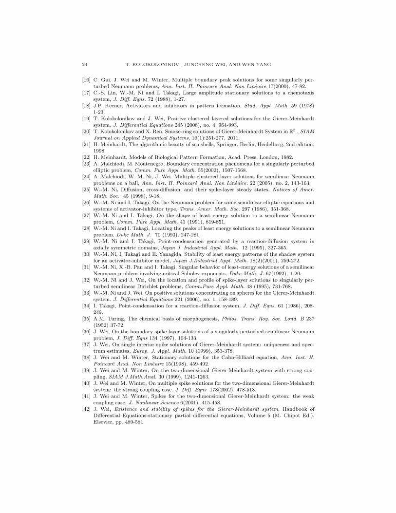
v

u

Figure 1. The ring solution to (1.1) with ε = 0.06. Dashed curvescorrespond to the asymptotic profile given in Theorem 1.1

In addition to the rigorous proof below, we also verify the formula (1.11) directlyby comparing it to the full numerical solution of (1.1). This is shown in Figure 1with ε = 0.06. The following table gives the data for a few additional values of ε :

ε rε (from full numerics) rε from (1.11 ) relative error

0.12 1.5414 1.5797 2.4%0.06 1.9701 2.0228 2.6%0.03 2.3917 2.4472 2.2%

Excellent agreement is observed.For concreteness, we limit this paper to the classical GM model p = 2, q = 1,m =

2, s = 0. However we expect the techniques to apply for more general p, q,m, s,provided that p = q + 1.

Acknowledgments. The research of the first author is supported by a grantfrom AARMS CRG in Dynamical Systems and NSERC grant 47050. He is is alsograteful for the hospitality of Juncheng Wei and CUHK, Mathematics department,where part of this paper was written. The research of the second author is partlysupported by a General Research Fund from RGC of Hong Kong.

2. outline of the proof of Theorem 1.1

Our strategy of the proof of the main results is based on the idea of solving thesecond equation in (1.1) for v and then working with a nonlocal elliptic PDE ratherthan directly with the system. This procedure is standard that have been used in[9], [19] and [33]. However, for the problem (1.1), the key function M(t) introduced


in [33] can be explicitly computed M(t) = 2e2t−1 . It is easy to see that the function

M(t) never possesses a zero point in t ∈ (0,+∞), as a result, we can not get thereduced problem solved. Instead, we need to give a more precise formula of theapproximate solution.

It’s convenient to rescale the problem by replacing the u by (εξ)−1u and v by(εξ)−1v, where ξ > 0 is to be chosen. (1.1) is transformed into the following radialform:

ε2(u′′ + 2ru′)− u+ u2

v= 0,

v′′ + 2rv′ − v + u2

εξ= 0,

(2.1)

where ξ =∫∞

0w2 is for convenience and we will give reason for this choice in

Appendix A.We consider a point t ∈ (0,+∞) which is a candidate for the location of con-

centration. Then we come to consider the second equation and by T[u2] we denotethe unique solution of the equation

v′′ +2

rv′ − v +

u2

εξ= 0. (2.2)

By using the Green function defined in (1.9), T[u2] can be written in the followingway:

T[u2](r) =1

εξ

∫ ∞

0

G(r, r′)u2(r′)dr′. (2.3)

Once we solved the second equation for v in (2.1) and scaling r = t+ εy, we getthe nonlocal PDE for u

u′′ +2ε

t+ εyu′ − u+

u2

T[u2](t+ εy)= 0, y ∈ (−

t

ε,+∞), u′(−

t

ε) = 0. (2.4)

By writing r′ = t+ εz, we have

v(y) =1

ξ

∫ ∞

0

G(t+ εy, t+ εz)u2(t+ εz)dz. (2.5)

We look for a solution to (2.4) in the form u = w( r−tε) + εU1 + φ, where U1 is

a function that will be introduced in Appendix A and φ is the perturbation term.Here we want to say more about the function U1. If we only use w( r−t

ε) + φ as

our approximate solution, the equation (2.4) would be transformed into a linearequation with respect to φ of order O(ε), and the reduced problem of this linearequation is to find the zero point of the function M(t) = 2

e2t−1 . ThoughM(t) never

vanishes in t ∈ (0,+∞), thanks to the fast decay property of this function M(t),we still can solve the equation (2.4) by giving a better approximation. Followingthis idea, we use U1 to cancel out the first order term appeared in the transformedequation of (2.4), in other words, if we use w( r−t

ε) + εU1 + φ as our approximate

solution, equation (2.4) will be transformed into a linear equation with respect toφ of order O(ε2). Then, by using the Lyapunov-Schmidt reduction, we can reducethis linear equation to a finite dimension problem which can be solved. Formally,we have

T[u2] = T[w2] + 2εT[wU1] + 2T[wφ] + ε2T[U21 ] + h.o.t., (2.6)

where h.o.t. corresponds to the higher order terms.


Using (2.5) and (2.6), we will prove in Section 4 that v can be written

v = 1 +

∫∞

−∞ wφ∫∞

0 w2+ εV1 + h.o.t., (2.7)

where V1 represents the ε−order term in the expansion of v, we will give a explicitformula for V1 in Appendix A. Then

u2

v= w2 + 2wφ−

∫∞

−∞ wφ∫∞

0 w2w2 − εV1w

2 + 2εwU1 + h.o.t.. (2.8)

Substituting all this in (2.4) we obtain the equation for φ

φ′′ +2ε

t+ εyφ′ − φ+ 2wφ−

2∫∞

−∞wφ

∫∞

−∞w2

w2 = Eε +Mε[φ], (2.9)

where Eε and Mε[φ] will be explicitly given in Section 5.Thus we have reduced the problem of finding solutions to (2.1) to a problem of

solving (2.9) for φ.Rather than directly solving problem (2.9), we consider first the following aux-

iliary problem: given any point t, find a function φ such that for certain constantsβε(t) the following equation is satisfied

Lε,tφ = Eε +Mε[φ] + βεww′,

∫

R

φww′ = 0, (2.10)

where

Lε,t[φ] := φ′′ +2ε

t+ εyφ′ − φ+ 2wφ−

2∫∞

−∞wφ

∫∞

−∞w2

w2.

We will prove in Section 3 and Section 5 that this problem is uniquely solvablewithin a class of small functions φ. We will then get a solution of the originalproblem when the point t is adjusted in such a way that βε(t) = 0. We show theexistence of such a point in Section 6, thereby proved Theorem 1.1. In Section 7,we will give a detail for computing U1 and V1. In Section 8, we list some numericalresults that would be used in Section 6 and Section 7.

3. linear problem

This section is devoted to a study of a linear problem, which reduces our problemto a one dimensional problem.

Let r1, r2 be a positive given number such that

r1 < t < r2, r1 = 1, r2 =1

ε2.

We set

Iε,t := (−t

ε,R− t

ε), (3.1)

where R = 3r2. Choose two fixed numbers R1 = r12 , R2 = 2r2. Let χ(s) be a

function such that χ(s) = 1 for s ∈ [R1,R2+r2

2 ] and χ(s) = 0 for s < R1

2 or s > R2.

Set

wε,t(y) = w(y)χ(t + εy), U1(y) = U1(y)χ(t+ εy). (3.2)


For u, v ∈ H1c (R

3), we equip them with the following scalar product:

(u, v)ε =

∫

Iε,t

(u′v′ + uv)(t+ εy)2dy (3.3)

(which is equivalent to the inner product of H1(R3).)Then orthogonality to the function w′

ε,t with respect to this scalar product isequivalent to the orthogonality to the function

Zε,t = w′′′ε,t +

2ε

t+ εyw′′

ε,t − w′ε,t (3.4)

in L2(Iε,t), equipped with the following scalar product

〈u, v〉ε =

∫

Iε,t

(uv)(t+ εy)2dy. (3.5)

(which is equivalent to the inner product of L2(R3).)Then we consider the following problem: for h ∈ L2 ∩L∞(Iε,t) being given, find

a function φ satisfying

Lε,t[φ] := φ′′ + 2εt+εy

φ′ − φ+ 2wε,tφ− 2

∫Iε,t

wε,tφ∫Iε,t

w2ε,t

w2ε,t = h+ cZε,t,

φ′(− tε) = 0, 〈φ, Zε,t〉ε = 0

(3.6)

for some constant c.Before we solve system (3.6), we need the following result which is just the

Lemma 5.1 in [33]. For convenience of the readers, we repeat the proof here.

Lemma 3.1. Let φ ∈ C2 (Iε,t) satisfy

|φ′′(y) +2ε

t+ εyφ′(y)− φ(y)| ≤ c0e

−µ|y|, φ′(−t

ε) = 0,

for some c0 > 0 and µ ∈ (0, 1). Then, provided that µ > 0 is sufficiently small,

|φ(y)| ≤ 2e2(|φ(0)|+ c0)e−µ|y|, ∀y ∈ Iε,t.

Proof. We use a comparison principle. Take η(t) a smooth cut-off function suchthat

η(t) = 1 for |t| ≤ 1, η(t) = 0 for |t| ≥ 2, 0 ≤ η ≤ 1.

Now consider the following auxiliary function:

Φ(y) = A[eµy + (eµy0 − eµy)η(µ(y +t

ε))],

where

y0 = −t

ε+

1

µ, A = 2e(|φ(0)|+ c0).

If y ∈ (− tε, y0), Φ(y) = Aeµy0 and hence

Φ′′ +2ε

t+ εyΦ′ − Φ = −Aeµy0 ≤ −c0e

µy.

If y ∈ (− tε+ 2

µ, 0), Φ(y) = Aeµy and ε

t+εy≤ µ

2 , hence

Φ′′ +2ε

t+ εyΦ′ − Φ ≤ A[2µ2 − 1]eµy ≤ −c0e

µy


provided that µ is sufficiently small. Finally it is easy to see that for y ∈ (y0, y0+1µ)

eµy0 ≤ eµy ≤ eeµy0 , Φ(y) ≥ Aeµy0 ,µ

2≤

ε

t+ εy≤ µ;

hence

Φ′′ +2ε

t+ εyΦ′ − Φ ≤CA(µ2)eµy −Aeµy0

≤CA(µ2)eµy −A

eeµy ≤ −c0e

µy

provided that µ is sufficiently small. Here C is a positive constant.In any case, we have that for y ∈ (− t

ε, 0), Φ(y) satisfies

Φ′′

+2ε

t+ εyΦ

′

− Φ ≤ −c0eµy, Φ

′

(−t

ε) = 0, Φ(0) ≥ |φ(0)|. (3.7)

Combining (3.7) with the hypothesis we obtain

(Φ− φ)′′(y) +2ε

t+ εy(Φ− φ)′(y)− (Φ− φ)(y) ≤ 0, ∀y ∈ [−

t

ε, 0] (3.8)

and

(Φ− φ)(0) > 0, (Φ− φ)′(−t

ε) = 0,

we claim that (Φ − φ)(y) ≥ 0 for y ∈ [− tε, 0). Assume the contrary, if we call

y the minimum point of Φ − φ in [− tε, 0), then it would be (Φ − φ)(y) < 0 and

(Φ−φ)′(y) = 0, (Φ−φ)′′(y) ≥ 0, in contradiction with (3.8). Hence we have provedthat φ ≤ Φ in [− t

ε, 0]. On the other hand by (3.8) and the hypothesis we also get

(Φ + φ)′′(y) +2ε

t+ εy(Φ + φ)′(y)− (Φ + φ)(y) ≤ 0 ∀y ∈ [−

t

ε, 0]

and (Φ + φ)(0) > 0, (Φ + φ)′(− tε) = 0. Proceeding as before we conclude φ ≥ −Φ

in [− tε, 0].

For y ∈ [0, R−tε

), we use Φ(y) = Acosh(µ(R−t

ε−y))

cosh(µ(R−t)ε

)as comparison function. Note

that Φ(0) = A, Φ′(R−tε

) = 0. It is easy to see that A2 e

−µy < Φ(y) < 2Ae−µy andhence

Φ′′ +2ε

t+ εyΦ′ − Φ ≤ −c0e

−µy

provided that µ is sufficiently small. By repeating the previous argument we obtain

|φ| ≤ Φ in [0, R−tε

) and the conclusion follows.

Let µ ∈ (0, 110 ) be a small number such that Lemma 3.1 holds. For every function

φ : Iε,t → R, we define

‖φ‖∗ = ‖eµ〈y〉φ(y)‖Iε,t , 〈y〉 = (1 + y2)12 . (3.9)

Since 2εt+εy

U ′′0 = O(ε)e−|y|, we obtain

Zε,t(y) = w′′′ − w′ +O(ε)e−µ〈y〉 = −2ww′ +O(ε)e−µ〈y〉 (3.10)

uniformly for t ∈ [R1, R2].The following proposition provides a priori estimates of φ satisfying (3.6).


Proposition 3.2. Let (φ, c) satisfy (3.6). Then for ε sufficiently small, r0 ∈[R1, R2], we have

‖φ‖∗ ≤ C‖h‖∗, (3.11)

where C is a positive constant depending on R,N only.

Remark. A more precise inequality should be

‖φ‖∗ ≤ C‖h⊥‖∗, where h⊥ = h−

〈h, Zε,t〉

〈Zε,t, Zε,t〉Zε,t. (3.12)

Proof. We prove the inequality by contradiction. Arguing by contradiction thereexists sequence εk → 0, tk ∈ [R1, R2] and a sequence of functions φεk,tk satisfying(3.6) such that the following holds

‖φεk,tk‖∗ = 1, ‖hk‖∗ = o(1),

∫

Iεk,tk

φεk,tkZεk,tk(tk + εky)2dy = 0.

For simplicity of notation, we drop the subindex k.Multiplying the first equation of (3.6) by w′

ε,t and integrating over Iε,t, we obtainthat

c

∫

Iε,t

Zε,tw′ε,t = −

∫

Iε,t

hw′ε,t +

∫

Iε,t

(Lε,t[φε,t]w′ε,t). (3.13)

The left-hand side of (3.13) equals c(−∫

Rpwp−1w′2 + o(1)) because of (3.10). The

first term on the right-hand side of (3.13) can be estimated by∫

Iε,t

hw′ε,t = O(‖h‖∗),

where we have used the fact that w is exponentially decay.The last term equals

∫

Iε,t

(Lε,t[φε,t])w′ε,t =

∫

Iε,t

[

φ′′ε,t +2ε

t+ εyφ′ε,t − φε,t + 2wε,tφε,t

]

w′ε,t

− 2

∫

Iε,twε,tφε,t

∫

Iε,tw2

ε,t

∫

Iε,t

w2ε,tw

′ε,t

=

∫

Iε,t

[

w′′′ε,t − w′

ε,t + 2wε,tw′ε,t

]

φε,t +O(ε‖φε,t‖∗)

=o(‖φε,t‖∗).

Hence we obtain that

|c| = O(‖h‖∗) + o(‖φε,t‖∗), ‖h+ cZε,t‖∗ = o(1). (3.14)

Next, we claim that ‖φε,t(y)‖ → 0 in any compact interval of R. In fact, we

consider φε(y) = φε,tχ(t + εy) where χ is the cut-off function introduced at the

beginning of the this section. Then since ‖φε,t‖∗ = 1, it is easy to see that ‖φε‖H2 ≤

C and hence φε → φ0 weakly in H2(R) and φ0 satisfies

φ′′0 − φ0 + 2wφ0 −2∫

Rwφ0

∫

Rw2

w2 = 0, |φ0| ≤ Ce−µ|y|.


By Lemma 4.2 in [33], we must have φ0 = cw′. On the other hand,∫

Iε,tφε,tZε,t(t+

εy)2dy = 0 and hence∫

Rφ0ww

′ = 0 which implies that c = 0 and hence φε,t → 0in any compact interval of R. This shows that

‖wε,tφε,t‖∗ = supy∈Iε,t

|eµ〈y〉wε,t(y)φε,t(y)| = o(1). (3.15)

On the other hand, by Lebesgue’s Dominated Convergence Theorem, we havethat

∫

Iε,t

wε,tφε,t → 0

which implies

‖

∫

Iε,twε,tφε,t

∫

Iε,tw2

ε,t

wε,t‖∗ = o(1). (3.16)

Thus we have arrived at the following situation φε,t satisfies

φ′′ε,t +2ε

t+ εyφ′ε,t − φε,t = o(eµ〈y〉), φ′ε,t(−

t

ε) = 0. (3.17)

Since φε,t → 0 in any compact interval, φε,t(0) = o(1). Applying Lemma 3.1,

we conclude that φε,t = o(eµ|y|). A contradiction to the assumption that ‖φ‖∗ = 1.This proves the proposition.

Finally, we have

Proposition 3.3. There exists an ε0 > 0 such that for any ε0 > 0 such that forany ε < ε0, t ∈ [R1, R2], given any h ∈ L2(Iε,t) ∩ L∞(Iε,t), there exists a uniquepair (φ, c) such that the following hold:

Lε,t[φ] = h+ cZε,t, φ′(−

t

ε) = 0, 〈φ, Zε,t〉ε = 0. (3.18)

Moreover, we have‖φ‖∗ ≤ C‖h‖∗. (3.19)

Proof. The existence follows from Fredholm alternatives. To this end, let us set

H = u ∈ H1(BR) | (u,w′ε,t)ε = 0.

Observe that φ solves (3.18) if only if φ ∈ H1(BR) satisfies∫

BR

(∇φ∇ψ + φψ) − 2〈wε,tφ, ψ〉ε − 2

∫

Iε,twε,tφ

∫

Iε,tw2

ε,t

〈w2ε,t, ψ〉ε = 〈h, ψ〉ε, ∀ψ ∈ H1(BR).

This equation can be rewritten in the following form:

φ+ S(φ) = h, (3.20)

where S is a linear compact operator from H to H, h = (∆ − 1)−1(h⊥) ∈ H andφ ∈ H.

Using Fredholm’s alternatives, we will show Eq.(3.20) has a unique solvablesolution for each h by proving that the equation has a unique solution for h = 0,i.e., h⊥ = 0. To this end, we assume the contrary. That is, there exists (φ, c) suchthat

Lε,t[φ] = cZε,t, φ′(−

t

ε) = 0, 〈φ, Zε,t〉ε = 0. (3.21)

From (3.21), it is easy to see that ‖φ‖∗ < +∞. So without loss of generality, wemay assume ‖φ‖∗ = 1. But then this contradicts (3.12).


4. Study of the operator T[h]

In this section, we study the operator T[h], where we choose h to be

h = (wε,t(r − t

ε) + εU1(

r − t

ε) + φ(

r − t

ε))2, ‖φ‖∗ = O(εσ), σ > 1. (4.1)

According the choice of h and the definition of operator T, we have

T[h](y) =1

ξ

∫ ∞

0

G(t+ εy, t+ εz)(wε,t(z) + εU1(z) + φ(z))2dz,

where ξ =∫∞

0 w2. From Appendix A, we can easily prove that U1 and w areexponential decay, therefore, we conclude

T[h](y) =1

ξ

∫ ∞

−∞

G(r0 + εy, r0 + εz)(wε,t(z) + εU1(z) + φ(z))2dz + o(ε3)

=1

ξ

∫ ∞

−∞

G(r0 + εy, r0 + εz)(w(z) + εU1(z) + φ(z))2dz + o(ε3). (4.2)

Define a by

e−2t = aε. (4.3)

Then we write

G(t+ εy, t+ εz) = G0 +

εG−1 + ε2G−

2 , y < z,

εG+1 + ε2G+

2 , y > z,(4.4)

where:

G0 =1

2, G−

1 = −a

2+ (y − z)(

1

2−

1

2t), G+

1 = −a

2+ (y − z)(−

1

2−

1

2t),

G−2 =

(y − z)2

4t2(y(t2 − 2t+ 2) + z(−t2 + 2t)) +

a

2t(y(t+ 1) + z(t− 1)),

G+2 =

(y − z)2

4t2(y(t2 + 2t+ 2) + z(−t2 − 2t)) +

a

2t(y(t+ 1) + z(t− 1)).

Substituting (4.3) and (4.4) into (4.2),

T[h](y) =1

ξ

∫ ∞

−∞

G0(w(z) + εU1(z) + φ(z))2dz

+1

ξ

∫ y

−∞

εG+1 (w(z) + εU1(z) + φ(z))2dz

+1

ξ

∫ ∞

y

εG−1 (w(z) + εU1(z) + φ(z))2dz

+1

ξ

∫ y

−∞

ε2G+2 (w(z) + εU1(z) + φ(z))2dz

+1

ξ

∫ ∞

y

ε2G−2 (w(z) + εU1(z) + φ(z))2dz + o(ε3)

=A1 +A2 +A3 +A4 +A5 + o(ε3). (4.5)


We study the terms Ai (i = 1, 2, 3, 4, 5) respectively in the following. For A1, wehave

A1 =1

ξ

∫ ∞

−∞

G0(w2 + 2wφ+ 2εwU1 + 2εU1φ+ ε2U2

1 + φ2)

=1 +1

ξ

∫ ∞

−∞

wφ+ε

ξ

∫ ∞

−∞

(wU1 + U1φ) +ε2

2ξ

∫ ∞

−∞

U21

+O(ε1+σ + ‖φ‖2∗), (4.6)

where we have used G0 = 12 and ‖φ‖∗ ≤ Cεσ, σ > 1. For A2 and A3, we have

A2 +A3 =ε

ξ(

∫ y

−∞

G+1 w

2 +

∫ ∞

y

G−1 w

2) +ε2

ξ(

∫ y

−∞

2G+1 wU1 +

∫ ∞

y

2G−1 wU1)

+O(ε1+σ + ‖φ‖2∗). (4.7)

For A4 and A5, we have

A4 +A5 =ε2

ξ(

∫ y

−∞

G+2 w

2 +

∫ ∞

y

G−2 w

2) +O(ε1+σ + ‖φ‖2∗). (4.8)

Combining (4.6)-(4.8), we get

T[h] =1 +1

ξ

∫ ∞

−∞

wφ+ εΘ1 +ε2

2ξ

∫ ∞

−∞

U21 +

ε2

ξ

∫ y

−∞

(2G+1 wU1 +G+

2 w2)

+ε2

ξ

∫ ∞

y

(2G−1 wU1 +G−

2 w2) +O(ε1+σ + ‖φ‖2∗), (4.9)

where

Θ1 =1

ξ(

∫ ∞

−∞

wU1 +

∫ y

−∞

G+1 w

2 +

∫ ∞

y

G−1 w

2).

From Appendix A, we can see Θ1 = V1. Summarizing the results, we obtain thefollowing lemma:

Lemma 4.1. For r = t+ εy, we have

T[(wε,t + εU1 + φ)2](t+ εy) =1 +1

ξ

∫ ∞

−∞

wφ+ εV1 +ε2

2ξ

∫ ∞

−∞

U21

+ε2

ξ

∫ y

−∞

(2G+1 wU1 +G+

2 w2)

+ε2

ξ

∫ ∞

y

(2G−1 wU1 +G−

2 w2)

+O(ε1+σ + ‖φ‖2∗). (4.10)


5. A nonlinear problem

In this section, we solve the following system of equation for (φ, β):

(wε,t + εU1 + φ)′′ +2ε

t+ εy(wε,t + εU1 + φ)′ − (wε,t + εU1 + φ)

+(wε,t + εU1 + φ)2

T[(wε,t + εU1 + φ)2]= βZε,t, (5.1)

with the following constrained condition

φ′(−t

ε) = 0,

∫

Iε,t

φZε,t(t+ εy)2dy = 0. (5.2)

The main result in this section is to show the following proposition

Proposition 5.1. For t ∈ [R1, R2] and ε sufficiently small, there exists a uniquepair (φε,t, βε,(t)) satisfying (5.1) and (5.2). Furthermore, (φε,t, βε,(t)) is continuousin t and we have the following estimate

‖φε,t‖∗ ≤ εσ, (5.3)

where σ ∈ (1, 2) is a constant.

Proof. We write (5.1) in the following form

Lε,t[φ] = Eε +Mε[φ] + βZε,t, (5.4)

where

Eε = −ε(U ′′1 − U1 + 2wε,tU1 +

2

tw′

ε,t − V1w2ε,t)− (w′′

ε,t − wε,t + w2ε,t), (5.5)

and

Mε[φ] =−

[

(wε,t + εU1 + φ)2

T[(wε,t + εU1 + φ)2]− w2

ε,t + 2

∫

Iε,twε,tφ

∫

Iε,tw2

ε,t

w2ε,t − 2wε,tφ+ εV1w

2ε,t

− 2εwε,tU1

]

+ (2ε

t−

2ε

t+ εy)w′

ε,t −2ε2

t+ εyU ′1

= M1ε[φ] +M

2ε[φ] +M

3ε[φ]. (5.6)

For Eε, it is easy to see

Eε =− ε(U ′′1 − U1 + 2wε,tU1 +

2

tw′

ε,t − V1w2ε,t)− (w′′

ε,t − wε,t + w2ε,t)

=− ε(U ′′1 − U1 + 2wU1 +

2

tw′ − V1w

2)− (w′′ − w + w2) +O(ε3e−µ〈y〉), (5.7)

where we have used the fact that U1, w are exponential decay and 0 < µ < 110 .

From Appendix A, we see U1 is just the solution to the following equation

U ′′1 − U1 + 2wU1 +

2

tw′ − V1w

2 = 0.

While w′′ − w + w2 = 0 holds for the setting of w. Hence, we conclude

‖Eε‖∗ ≤ Cε3. (5.8)


For Mε, using (4.10), we can write(wε,t+εU1+φ)2

T[(wε,t+εU1+φ)2]as

(wε,t + εU1 + φ)2

T[(wε,t + εU1 + φ)2]=w2

ε,t + 2εwε,tU1 − εV1w2ε,t + 2wε,tφ−

∫∞

−∞wφ

ξw2

ε,t + ε2U21

+ ε2w2ε,tV

21 − 2ε2wε,tU1V1 − ε2Θ2w

2ε,t +O(ε2+δ), (5.9)

where

Θ2 =ε2

2ξ

∫ ∞

−∞

U21 +

ε2

ξ

∫ y

−∞

(2G+1 wU1 +G+

2 w2) +

ε2

ξ

∫ ∞

y

(2G−1 wU1 +G−

2 w2).

Substituting (5.9) into M1ε, we obtain

‖M1ε[φ]‖∗ ≤ C(ε2 + ‖φ‖2∗), (5.10)

where we have used U1 and w are exponential decay. For the another two terms, itis not difficult to find that

‖M2ε[φ]‖∗ + ‖M3

ε[φ]‖∗ ≤ Cε2. (5.11)

Combining (5.10) and (5.11), we get ‖Mε[φ]‖∗ ≤ C(‖φ‖2∗ + ε2).Set B = φ ∈ H | ‖φ‖∗ < Cεσ. Fix φ ∈ B and let Aε be the unique map h→ φ

given by Proposition 3.3. Defining

Gε = Aε(Eε +Mε[φ]).

We now show that Gε is a contraction map. In fact, by Proposition 3.3, we have

‖Gε[φ]‖∗ ≤ C‖Eε +Mε[φ]‖∗ ≤ Cε2 + ε2σ ≤ Cε2, (5.12)

since 1 < σ < 2, and hence Gε[φ] ∈ B. Moreover, we also have

‖Gε[φ1]− Gε[φ2]‖∗ ≤C‖Mε[φ1]−Mε[φ2]‖

≤C(ε+ ‖φ1‖∗ + ‖φ2‖∗)‖φ1 − φ2‖∗. (5.13)

Eq. (5.12) and (5.13) show that the map Gε is a contraction map from B to B. Bythe contraction mapping theorem, (5.4) has a unique solution φ ∈ B, called φε,t.

The continuity of (φε,t, βε(t)) follows from the uniqueness of (φε,t, βε(t)).

6. The reduced problem

In this section we solve the reduced problem and prove our main result. Inparticular, we obtain that

Proposition 6.1. For ε sufficiently small, βε(t) is continuous in t and we have

βε(t) =b0

tε2(

309

700−

3

5ta−

3

10a) + o(ε2+δ), (6.1)

where b0 6= 0 is some generic constant and δ ∈ (0, σ).

From Proposition 6.1, we can finish the proof of Theorem 1.1.


Proof of Theorem 1.1. Since ε−2b−10 βε(t) = 1

t(309700 − 3

5 ta − 310a) + o(εδ). On the

other hand, we have a = e−2t

ε. Then we can write

b−10 ε−2βε(t) =

1

t(309

700−

3

10

(2t+ 1)e−2t

ε) + o(εδ). (6.2)

For ε sufficiently small. From Section 3, we have 1 < t < 1ε2. If we choose t = 2, we

can make the right hand side of (6.2) negative. While if we choose t = −2 ln(ε) < 1ε2

we can make the right hand side of (6.2) positive. By the continuity of βε(t) andthe mean value theorem, a zero of βε, denoted by tε, is thus guaranteed, whichproduces a solution uε = wε,t + εU1 + φε,t to (5.1) and (5.2). It is easy to verifythat uε satisfies all the properties of Theorem 1.1.

We now prove Proposition 6.1. Observing that φε,t satisfies (5.4). MultiplyingEq.(5.4) by w′

ε,t and integrating by over Iε,t, we obtain

βε(t)

∫

Iε,t

Zε,tw′ε,t =

∫

Iε,t

Lε,t[φε,t]w′ε,t +

∫

Iε,t

(−Eεw′ε,t) +

∫

Iε,t

(−Mε[φε,t]w′ε,t).

(6.3)

The left hand side of (6.3) can be computed as:

βε(t)

∫

Iε,t

Zε,tw′ε,t = −2βε(t)

∫

R

(w(w′)2) +O(εβε(t)). (6.4)

We estimate each term on the right hand side of (6.3). For the first term, we useintegration by parts:

∫

Iε,t

Lε,t[φε,t]w′ε,t =

∫

Iε,t

[φ′′ε,t − φε,t + 2wε,tφε,t]w′ε,t +O(ε‖φε,t‖∗)

=

∫

Iε,t

[w′′′ε,t − w′

ε,t + 2wε,tw′ε,t]φε,t = O(ε1+σ). (6.5)

The second term in (6.3) gives, using (5.8),∫

Iε,r0

EεU′0 = O(ε3). (6.6)

It remains to compute the third term on the right hand side of (6.3), by (5.9),

(wε,t + εU1 + φ)2

T[(wε,t + εU1 + φ)2]=w2

ε,t + 2εwε,tU1 − εV1w2ε,t + 2wε,tφ−

∫∞

−∞wφ

ξw2

ε,t + ε2U21

+ ε2w2ε,tV

21 − 2ε2wε,tU1V1 − ε2Θ2w

2ε,t +O(ε2+δ), (6.7)

we can write Mε as

Mε[φ] =ε2[

−2

tU ′1 +

2y

t2w′

ε,t + w2ε,tΘ2 + 2wε,tU1V1 − U2

1 − w2ε,tV

21

]

+ (2ε

t−

2ε

t+ εy−

2yε2

t2)w′

ε,t + (2ε2

t−

2ε2

t+ εy)U ′

1 + o(ε2+σ)

=ε2[

−2

tU ′1 +

2y

t2w′ + w2Θ2 + 2wU1V1 − U2

1 − w2V 21

]

+ o(ε2+δ), (6.8)

where we used that fact that w, U1 are exponential decay.


Next, we consider the term

Π = −2

tU ′1 +

2y

t2w′ + w2Θ2 + 2wU1V1 − U2

1 − w2V 21 .

Specifically, we need to compute the inner product of Π and w′ε,t, and we find

∫ ∞

−∞

Πw′ε,t =

∫ ∞

−∞

Πw′ +O(ε3).

Therefore, it is only necessary to compute∫∞

−∞ Πw′. From Appendix A, we see

Θ2 = V2 −1

ξ

∫ ∞

−∞

wU2,

where U2, V2 represent the ε2−order term in the expansion of u, v respectively.Then we find∫ ∞

−∞

Πw′ =

∫ ∞

−∞

[

2

tU1(w − w2)−

1

3w3V ′

2 + 2ww′U1V1 − U21w

′ − w2w′V 21

]

, (6.9)

where we used the fact∫ ∞

−∞

yw′2 = 0,

∫ ∞

−∞

w2w′ = 0, w′′ − w + w2 = 0.

It is to check (6.9) is just the following one

2

t(I1 − I2)−

1

3I3 + 2I4 − I5 − I6,

where

I1 =

∫ ∞

0

U1evenw, I2 =

∫ ∞

0

U1evenw2, I3 =

∫ ∞

0

w3(V ′2 )even,

I4 =1

2

∫ ∞

−∞

ww′U1V1 =

∫ ∞

−∞

ww′[U1evenV1odd + V1evenU1odd],

I5 =1

2

∫ ∞

−∞

w′U21 = 2

∫ ∞

0

w′(U1evenU1odd),

I6 =1

2

∫ ∞

−∞

w2w′V 21 = 2

∫ ∞

0

w2w′(V1evenV1odd),

where U1even stands for the even function part of U1, U1odd stands for the oddfunction part of U1(same notation for U0, U2, V0, V1, V2).

By (7.9), we have

I1 − I2 =

∫ ∞

0

(C0w − φ1)(w − w2) = −3

5C0 +

∫ ∞

0

φ1w2 −

∫ ∞

0

φ1w (6.10)

and

I3 =

∫ ∞

−∞

w3(a−C0

t+

1

t(2ρ(y) + 3

∫∞

0zw2

∫∞

0w2

− 2

∫ y

0zw2

∫∞

0w2

− 2w2

∫∞

0w2

))

=(a−C0

t+

1

t

∫ ∞

0

zw2)

∫ ∞

−∞

w3 −2

3t

∫ ∞

0

w3(

∫ y

0

zw2dz)dy

−2

3t

∫ ∞

0

w5 +2

t

∫ ∞

0

w3ρ, (6.11)


where ρ(y), φ1, C0 will be given in Appendix A and we have used∫∞

0w2 = 3 (this

identity will be given in Appendix B). Thus, we obtain

I1 − I2 −t

6I3 =

∫ ∞

0

φ1w2 −

∫ ∞

0

φ1w −3

5(ta+

∫ ∞

0

zw2) +1

9

∫ ∞

0

w3(

∫ y

0

zw2dz)dy

+1

9

∫ ∞

0

w5 −1

3

∫ ∞

0

w3ρ. (6.12)

Then, in Appendix B, we show

I1 − I2 −t

6I3 = −

57

100−

3

5ta. (6.13)

On the other hand, we have

I4 = −2

tC0

∫ ∞

0

ww′(w′ + yw) +1

t

∫ ∞

0

ww′[yφ1 + (2w′ + yw)ρ],

I5 = −2

t

∫ ∞

0

w′(C0w − φ1)(2w′ + yw), I6 = −

2

t

∫ ∞

0

yww′(C0 − ρ).

Hence,

−t

2(I5 + I6 − 2I4) =−

∫ ∞

0

2w′2φ1 +

∫ ∞

0

ww′(2w′ + yw − y)ρ

+ C0

∫ ∞

0

yww′(1− w). (6.14)

Further, we will show in Appendix B

−t

2(I5 + I6 − 2I4) =

177

175−

3

10a. (6.15)

Combining (6.7)-(6.15), we get∫ ∞

−∞

Mε,tw′ε,t =

2

tε2(

309

700−

3

5ta−

3

10a) + o(ε2+δ). (6.16)

By (6.3)-(6.6) and (6.16), we have

βε(t) =b0

tε2(

309

700−

3

5ta−

3

10a) + o(ε2+δ). (6.17)

Therefore, we get the proposition proved.

7. Appendix A

In this appendix, we compute the explicit expressions of the first and secondapproximation of u and v. Let U(y) = u(r), V (y) = v(r), y = r−t

ε. We formally

write U, V into the following

U = U0 + εU1 + ε2U2 + · · · ; V = V0 + εV1 + ε2V2 + · · · .

By (2.3), we have

V (y) ∼1

ξ

∫ ∞

−∞

G(r0 + εy, r0 + εz)U2(z)dz. (7.1)


At leading order, we then get

V0 =G0

ξ

∫ ∞

−∞

U20 ; U ′′

0 − U0 +U20

V0= 0,

where we used the expansion of G in (4.4). We now choose the constant ξ so thatV0 = 1 and therefore U0 = w; that is

ξ =

∫ ∞

0

w(y)2dy; V0 = 1; U0 = w.

Next, after computing all the terms up to O(ε2) in (2.1), we obtain

L0U1 +2

tU ′0 − U2

0V1 = 0,

L0U2 +2

tU ′1 −

2y

r20U ′0 − U2

0V2 − 2U0U1V1 + U21 + U2

0V21 = 0,

V ′′1 +

1

ξU20 = 0,

V ′′2 +

2

tV ′1 − 1 +

2

ξU0U1 = 0, (7.2)

where the operator L0 is defined as L0ψ = (∂2 − 1 + 2U0)ψ. Multiplying the firstequation in (7.2) by U ′

0, we get

2

t

∫ ∞

−∞

U ′20 +

1

3

∫ ∞

−∞

U30V

′1 = 0. (7.3)

From (7.1), we have

ξV1 = 2G0

∫ ∞

−∞

U0U1dz +

∫ y

−∞

G+1 (y, z)U

20 (z)dz +

∫ ∞

y

G−1 (y, z)U

20 (z)dz. (7.4)

Differentiating the both two sides with respect to y, we get

ξV ′1 =

∫ y

−∞

(−1

2−

1

2t)U2

0 (z)dz +

∫ ∞

y

(1

2−

1

2t)U2

0 (z)dz

=−1

2t

∫ ∞

−∞

U20 (z)dz + f1,

where f1 is an odd function of y. In addition, we can write

V ′1 = −

1

t+ f2, f2 is an odd function of y.

Then, the left hand side of (7.3) becomes

2

t

∫ ∞

−∞

U ′20 −

1

3t

∫ ∞

−∞

U30 = 0.

This expression is identically zero, since∫∞

−∞ U ′20 = 6

5 and∫∞

−∞ U30 = 36

5 . These two

identities can be directly proven by using w(y) = 32 sech

2(y2 ).Next we consider the function V2. From (7.1), we have

ξV2 =

∫ ∞

−∞

G2U20 +

∫ ∞

−∞

2G1U0U1 +

∫ ∞

−∞

G0(U21 + 2U0U2). (7.5)


Actually we only care about the even part of V ′2 . We have

ξV ′2 =[G+

2 (y, y)−G−2 (y, y)]U

20 +

∫ y

−∞

G+2yU

20 +

∫ ∞

y

G−2yU

20

+ 2[G+1 (y, y)−G−

1 (y, y)]U0U1 +

∫ y

−∞

2G+1yU0U1 +

∫ ∞

y

2G−1yU0U1, (7.6)

where G+2y =

∂G+2

∂y, similar notation will be used for G+

1 , G−1 , G

−2 respectively. Since

G+2 (y, y)−G−

2 (y, y) = G+1 (y, y)−G−

1 (y, y) = 0,

(7.6) becomes

ξV ′2 =

∫ y

−∞

G+2yU

20 +

∫ ∞

y

G−2yU

20 +

∫ y

−∞

2G+1yU0U1 +

∫ ∞

y

2G−1yU0U1. (7.7)

Now we evaluate the first two terms on the right hand side of (7.7), keeping onlythe even terms in y. We have

G−2y =

1

2t2(y + (y − z)(t− 1)2) +

a

2t(t+ 1),

G+2y =

1

2t2(y + (y − z)(t+ 1)2) +

a

2t(t+ 1),

then∫ y

−∞

G+2yU

20 +

∫ ∞

y

G−2yU

20 =

∫ y

0

G+2yU

20 +

∫ 0

y

G−2yU

20 +

∫ 0

−∞

G+2yU

20 +

∫ ∞

0

G−2yU

20 ,

∫ 0

−∞

G+2yU

20 +

∫ ∞

0

G−2yU

20 = a(1 +

1

t)

∫ ∞

0

U20 +

2

t

∫ ∞

0

zU20 + f3,

and∫ y

0

G+2yU

20 +

∫ 0

y

G−2yU

20 =

2

t

∫ y

0

(y − z)U20 ,

where f3 is an odd function of y. So that∫ y

−∞

G+2yU

20 +

∫ ∞

y

G−2yU

20 = a(1 +

1

t)

∫ ∞

0

U20 +

2

t

∫ ∞

0

zU20 +

2

t

∫ y

0

(y − z)U20 + f3.

Next we compute the terms involving U1. We can write∫ y

−∞

2G+1yU0U1 +

∫ ∞

y

2G−1yU0U1 =

∫ 0

−∞

2G+1yU0U1 +

∫ ∞

0

2G−1yU0U1

+

∫ y

0

2G+1yU0U1 +

∫ 0

y

2G−1yU0U1. (7.8)

Since G−1y = (12 − 1

2t ) and G+1y = (− 1

2 − 12t ), we get

∫ 0

−∞

2G+1yU0U1 +

∫ ∞

0

2G−1yU0U1 =

∫ 0

−∞

(−1−1

t)U0U1 +

∫ ∞

0

(1−1

t)U0U1

=−2

t

∫ ∞

0

U0U1even + 2

∫ ∞

0

U0U1odd,


and∫ y

0

2G+1yU0U1 +

∫ 0

y

2G−1yU0U1 =

∫ y

0

(1

t− 1)U0U1odd −

∫ y

0

(1

t+ 1)U0U1odd + f4

=− 2

∫ y

0

U0U1odd + f4,

where f4 is a odd function of y. Let’s define ρ(y) :=∫

y

0(y−z)U2

0dz

ξ. Then we have

(V ′2 )even =a(1 +

1

t) +

2

tξ

∫ ∞

0

zU20 +

2

tρ(y)−

2

tξ

∫ ∞

0

U0U1even

+2

ξ

∫ ∞

0

U0U1odd −2

ξ

∫ y

0

U0U1odd.

Next, we compute U1, V1 explicitly. We have

ξV1 =

∫ ∞

−∞

U0(z)U1(z)dz +

∫ ∞

0

G−1 U

20 +

∫ 0

−∞

G+1 U

20 +

∫ 0

y

G−1 U

20 +

∫ y

0

G+1 U

20 ,

∫ 0

−∞

G+1 U

20 +

∫ ∞

0

G−1 U

20 = −

y

t

∫ ∞

0

U20 +

∫ ∞

0

(−zU20 − aU2

0 ),

∫ y

0

G+1 U

20 +

∫ 0

y

G−1 U

20 = −

∫ y

0

(y − z)U20 .

So that

V1 = −y

t− a−

1

ξ

∫ ∞

0

zU20 − ρ(y) +

1

ξ

∫ ∞

−∞

U0(z)U1(z)dz.

Separating the odd and even part of V1 and U1, we find

V1odd = −y

t, V1even = −a−

1

ξ

∫ ∞

0

zU20 − ρ(y) +

2

ξ

∫ ∞

0

U0U1even,

U1odd and U1even satisfies

L0U1odd +2

tU ′0 +

y

tU20 = 0,

L0U1even − U20 (−a−

1

ξ

∫ ∞

0

zU20 − ρ(y) +

2

ξ

∫ ∞

0

U0U1even) = 0.

Therefore

U1even =

(

− a−1

ξ

∫ ∞

0

zU20 +

2

ξ

∫ ∞

0

U0U1even

)

U0 − L−10 (U2

0 ρ),

U1odd = −y

tU0 −BU ′

0,

where B is defined later. Now we can get∫ ∞

0

U0U1even = −a

∫ ∞

0

U20 −

∫ ∞

0

zU20 + 2

∫ ∞

0

U0U1even −

∫ ∞

0

U0L−10 (U2

0 ρ),

so that∫ ∞

0

U0U1even = a

∫ ∞

0

U20 +

∫ ∞

0

zU20 +

∫ ∞

0

U0L−10 (U2

0 ρ).

As a consequence,

U1even =

(

a+1

ξ

∫ ∞

0

zU20 +

2

ξ

∫ ∞

0

U0L−10 (U2

0 ρ)

)

U0 − L−10 (U2

0 ρ).


To get the constant B, we impose U ′1(0) = 0. We have

−U ′1(0) =

1

tU0(0) +BU ′′

0 (0) =1

t

3

2+B(

3

2−

9

4) = 0,

so that B = 2t. Then we obtain

U1odd = −1

t(2U ′

0 + yU0).

Combining the formula of U1even and V1even, we get

V1even = a+1

ξ

∫ ∞

0

zU20 − ρ(y) +

2

ξ

∫ ∞

0

U0L−10 (U2

0 ρ).

Next we simplify (V ′2)even as follows. First, we have

∫ ∞

0

U0U1even = a

∫ ∞

0

U20 +

∫ ∞

0

zU20 +

∫ ∞

0

U0L−10 (U2

0 ρ),

∫ y

0

U0U1odd = −1

t(U2

0 −9

4+

∫ y

0

zU20 ),

∫ ∞

0

U0U1odd = −1

t(−

9

4+

∫ ∞

0

zU20 ).

Then, we define

ρ(y) :=1

ξ

∫ y

0

(y − z)U20 , φ1 = L−1

0 (U20 ρ), C0 := a+

1

ξ

∫ ∞

0

zU20 +

2

ξ

∫ ∞

0

U0φ1.

Summarizing our results, which are the following

U1even = C0U0 − φ1, U1odd = −1

t(2U ′

0 + yU0),

V1even = C0 − ρ(y), V1odd = −y

t,

V2y,even = a−C0

t+

1

t

(

2ρ(y) +3

ξ

∫ ∞

0

zU20 −

2

ξ

∫ y

0

zU20 −

2

ξU20

)

. (7.9)

8. Appendix B

In this appendix we compute explicitly the expressions (6.13) and (6.15). Weclaim

I1 − I2 −t

6I3 = −

57

100−

3

5ta, (8.1)

−t

2(I5 + I6 − 2I4) =

177

175−

3

10a. (8.2)

Let’s define

J(p) :=

∫ ∞

0

wpρ, K(p) :=

∫ ∞

−∞

wpρy, M(p) :=

∫ ∞

0

wp,

where ρ = 13

∫ y

0 (z − y)w2(z)dz. Using the equations

w′′ − w + w2 = 0, w′2 − w2 +2

3w3 = 0, ρyy =

1

3w2,


we derive the following recursion identities

J(p) =3(p− 1)

2p− 1J(p− 1)−

1

(p− 1)(2p− 1)M(p+ 1), p > 1, (8.3)

K(p) =3(p− 1)

2p− 1K(p− 1)−

2p

(p+ 1)(p− 1)(2p− 1)M(p+ 1), p > 1, (8.4)

M(p) =3(p− 1)

2p− 1M(p− 1), p > 1. (8.5)

The proof of (8.3)-(8.5) are directly and we omit the details. Using (8.3)-(8.5), weobtain the following table

i 1 2 3 4 5

M(i) 3 3 185

16235

21635

K(i) 72

1910

11170

J(i) 132 − 6 ln(2) 53

10 − 6 ln(2) 1032175 − 36

5 ln(2) 89281225 − 324

35 ln(2)In addition we evaluate

∫ ∞

0

zw2 = −3

2+ 6 ln(2),

∫ ∞

0

w3(

∫ y

0

zw2dz) = −4527

350+

108

5ln(2). (8.6)

We now compute

∫ ∞

0

φ1w2 =

∫ ∞

0

w3ρ = J(3) =1032

175−

36

5ln(2) (8.7)

∫ ∞

0

φ1w =

∫ ∞

0

w2ρ(w +1

2yw′) =

∫ ∞

0

w3ρ+1

6

∫ ∞

0

y(w3)′ρ

=

∫ ∞

0

5

6w3ρ−

∫ ∞

0

1

6w3yρ′ =

5

6J(3)−

1

6K(3)

=93

20− 6 ln(2). (8.8)

To evaluate∫∞

0w′2φ1, we note

L0w2 = 2w′′w + 2w′2 − w2 + 2w3 = 2w′2 + w2,

so that L−10 w′2 = 1

2 (w2 − w). Thus

−

∫ ∞

0

2w′2φ1 = −

∫ ∞

0

(w2 − w)ρ =

∫ ∞

0

w′′ρ =1

3

∫ ∞

0

w3 =6

5. (8.9)

Finally, we get

C0 = a+1

3

∫ ∞

0

zw2 +2

3

∫ ∞

0

wφ1 = a+13

5− 2 ln(2), (8.10)

∫ ∞

0

yww′(1− w) =

∫ ∞

0

yw′′w′ = −1

2

∫ ∞

0

w′2 = −3

10, (8.11)


∫ ∞

0

ww′(2w′ + yw − y)ρ =

∫ ∞

0

2w′2wρ− yw′w′′ρ

=

∫ ∞

0

(2(w2 −2

3w3)wρ+

1

2w′2(ρ+ yρy))

=

∫ ∞

0

(2w3 −4

3w4)ρ+

∫ ∞

0

(1

2w2 −

1

3w3)(ρ+ yρy)

=1

2J(2) +

5

3J(3)−

4

3J(4) +

1

2K(2)−

1

3K(3)

=7797

2450−

93

35ln(2). (8.12)

Then, using (8.3)-(8.12), we get the claim proved.

References

[1] A.Ambrosetti, A. Malchiodi and W.-M. Ni, Singularly perturbed elliptic equations with sym-metry: existence of solutions concentrating on spheres, Part I, Comm. Math. Phys. 235(2003), no. 3, 427-466.

[2] A.Ambrosetti, A. Malchiodi and W.-M. Ni, Singularly perturbed elliptic equations with sym-metry: existence of solutions concentrating on spheres, Part II, Indiana Univ. Math. J. 53(2004), no. 2, 297-329.

[3] Adimurthi, G. Mancini, and S.L. Yadava, The role of mean curvature in a semilinear Neumannproblem involving the critical Sobolev exponent, Comm. P.D.E. 20(1995), 591-631.

[4] Adimurthi, F. Pacella, and S.L. Yadava, Interaction between the geometry of the boundaryand positive solutions of a semilinear Neumann problem with critical nonlinearity, J. Funct.Anal. 113 (1993), 318-350.

[5] M. Abramowitz and I.A. Stegun, Handbook of Mathematical Functions with Formulas,Graphs, and Mathematical Tables, Washington, National Bureau of Standards Applied Math-ematics, 1964.

[6] P. Bates and G. Fusco, Equilibria with many nuclei for the Cahn-Hilliard equation, J. Diff.Eqns. 4(1999),1-69.

[7] E.N. Dancer and S. Yan, Multipeak solutions for a singular perturbed Neumann problem,Pacific J. Math. 189(1999), 241-262.

[8] M. del Pino, M. Kowalczyk and X. Chen, The Gierer-Meinhardt system: the breaking ofsymmetry of homoclinics and multi-bump ground states, Comm. Contemp. Math. , 3 (3),(2001) 419–439.

[9] M. del Pino, M. Kowalczyk and J. Wei, Multi-bump ground states of the Gierer-Meinhardtsystem in R

2, Ann. Inst. H. Poincare Anal. Non Lineaire 20(2003), 53-85.[10] M. del Pino, M. Kowalczyk and J. Wei, Concentration on curves for nonlinear Schr?dinger

equations. Comm. Pure Appl. Math. 60 (2007), no. 1, 113-146.[11] A. Doelman, R. A. Gardner and T.J. Kaper, Large stable pulse solutions in reaction-diffusion

equations, Indiana Univ. Math. J 50 (1), (2001) 443–507.[12] A. Doelman, T.J. Kaper, and H. van der Ploeg, Spatially periodic and aperiodic multi-pulse

patterns in the one-dimensional Gierer-Meinhardt equation, Methods Appl. Anal. 8(2001),387-414.

[13] C. Ghoussoub and C. Gui, Multi-peak solutions for a semilinear Neumann problem involvingthe critical Sobolev exponent, Math. Z. 229 (1998), 443–474.

[14] A. Gierer and H. Meinhardt, A theory of biological pattern formation, Kybernetik (Berlin)12 (1972), 30-39.

[15] C. Gui and J. Wei, Multiple interior peak solutions for some singular perturbation problems,J. Diff. Eqns. 158(1999), 1-27.


[16] C. Gui, J. Wei and M. Winter, Multiple boundary peak solutions for some singularly per-turbed Neumann problems, Ann. Inst. H. Poincare Anal. Non Lineaire 17(2000), 47-82.

[17] C.-S. Lin, W.-M. Ni and I. Takagi, Large amplitude stationary solutions to a chemotaxissystem, J. Diff. Eqns. 72 (1988), 1-27.

[18] J.P. Keener, Activators and inhibitors in pattern formation, Stud. Appl. Math. 59 (1978)1-23.

[19] T. Kolokolonikov and J. Wei, Positive clustered layered solutions for the Gierer-Meinhardtsystem. J. Differential Equations 245 (2008), no. 4, 964-993.

[20] T. Kolokolonikov and X. Ren, Smoke-ring solutions of Gierer-Meinhardt System in R3 , SIAM

Journal on Applied Dynamical Systems, 10(1):251-277, 2011.[21] H. Meinhardt, The algorithmic beauty of sea shells, Springer, Berlin, Heidelberg, 2nd edition,

1998.[22] H. Meinhardt, Models of Biological Pattern Formation, Acad. Press, London, 1982.[23] A. Malchiodi, M. Montenegro, Boundary concentration phenomena for a singularly perturbed

elliptic problem, Comm. Pure Appl. Math. 55(2002), 1507-1568.[24] A. Malchiodi, W. M. Ni, J. Wei. Multiple clustered layer solutions for semilinear Neumann

problems on a ball, Ann. Inst. H. Poincare Anal. Non Lineaire. 22 (2005), no. 2, 143-163.[25] W.-M. Ni, Diffusion, cross-diffusion, and their spike-layer steady states, Notices of Amer.

Math. Soc. 45 (1998), 9-18.

[26] W.-M. Ni and I. Takagi, On the Neumann problem for some semilinear elliptic equations andsystems of activator-inhibitor type, Trans. Amer. Math. Soc. 297 (1986), 351-368.

[27] W.-M. Ni and I. Takagi, On the shape of least energy solution to a semilinear Neumannproblem, Comm. Pure Appl. Math. 41 (1991), 819-851.

[28] W.-M. Ni and I. Takagi, Locating the peaks of least energy solutions to a semilinear Neumannproblem, Duke Math. J. 70 (1993), 247-281.

[29] W.-M. Ni and I. Takagi, Point-condensation generated by a reaction-diffusion system inaxially symmetric domains, Japan J. Industrial Appl. Math. 12 (1995), 327-365.

[30] W.-M. Ni, I. Takagi and E. Yanagida, Stability of least energy patterns of the shadow systemfor an activator-inhibitor model, Japan J.Industrial Appl. Math. 18(2)(2001), 259-272.

[31] W.-M. Ni, X.-B. Pan and I. Takagi, Singular behavior of least-energy solutions of a semilinearNeumann problem involving critical Sobolev exponents, Duke Math. J. 67(1992), 1-20.

[32] W.-M. Ni and J. Wei, On the location and profile of spike-layer solutions to singularly per-turbed semilinear Dirichlet problems, Comm.Pure Appl. Math. 48 (1995), 731-768.

[33] W.-M. Ni and J. Wei, On positive solutions concentrating on spheres for the Gierer-Meinhardtsystem. J. Differential Equations 221 (2006), no. 1, 158-189.

[34] I. Takagi, Point-condensation for a reaction-diffusion system, J. Diff. Eqns. 61 (1986), 208-249.

[35] A.M. Turing, The chemical basis of morphogenesis, Philos. Trans. Roy. Soc. Lond. B 237(1952) 37-72.

[36] J. Wei, On the boundary spike layer solutions of a singularly perturbed semilinear Neumannproblem, J. Diff. Eqns 134 (1997), 104-133.

[37] J. Wei, On single interior spike solutions of Gierer-Meinhardt system: uniqueness and spec-trum estimates, Europ. J. Appl. Math. 10 (1999), 353-378.

[38] J. Wei and M. Winter, Stationary solutions for the Cahn-Hilliard equation, Ann. Inst. H.Poincare Anal. Non Lineaire 15(1998), 459-492.

[39] J. Wei and M. Winter, On the two-dimensional Gierer-Meinhardt system with strong cou-pling, SIAM J.Math.Anal. 30 (1999), 1241-1263.

[40] J. Wei and M. Winter, On multiple spike solutions for the two-dimensional Gierer-Meinhardtsystem: the strong coupling case, J. Diff. Eqns. 178(2002), 478-518.

[41] J. Wei and M. Winter, Spikes for the two-dimensional Gierer-Meinhardt system: the weakcoupling case, J. Nonlinear Science 6(2001), 415-458.

[42] J. Wei, Existence and stability of spikes for the Gierer-Meinhardt system, Handbook ofDifferential Equations-stationary partial differential equations, Volume 5 (M. Chipot Ed.),Elsevier, pp. 489-581.


Department of Mathematics, Dalhousie University, Canada

Department of Mathematics, The Chinese University of Hong Kong, Shatin, Hong

Kong

E-mail address: [email protected]

Department of Mathematics, The Chinese University of Hong Kong, Shatin, Hong

Kong

E-mail address: [email protected]

ON LARGE RING SOLUTIONS FOR GIERER-MEINHARDT SYSTEM …jcwei/gm-largering-10-11-12.pdf · ON LARGE...

Documents

Transcript of ON LARGE RING SOLUTIONS FOR GIERER-MEINHARDT SYSTEM …jcwei/gm-largering-10-11-12.pdf · ON LARGE...