ON INTRINSIC NONLINEAR PARTICLE MOTION IN COMPACT...
123
ON INTRINSIC NONLINEAR PARTICLE MOTION IN COMPACT SYNCHROTRONS Kilean Hwang Submitted to the faculty of the University Graduate School in partial fulfillment of the requirement for the degree Doctor of Philosophy in the Department of Physics, Indiana University April, 2016
Transcript of ON INTRINSIC NONLINEAR PARTICLE MOTION IN COMPACT...
ON INTRINSIC NONLINEAR PARTICLE
MOTION IN COMPACT SYNCHROTRONS
Kilean Hwang
Submitted to the faculty of the University Graduate School
in partial fulfillment of the requirement
for the degree
Doctor of Philosophy
in the Department of Physics,
Indiana University
April, 2016

ii
Accepted by the Graduate Faculty, Indiana Univeristy, in partial fulfillment of the
requirement for the degree of Doctor of Philosophy.
Shyh-Yuan Lee, Ph.D.
John Carini, Ph.D.
Doctoral
Committee
Rex Tayloe, Ph.D.
July 23th, 2015 W. Michael Snow, Ph.D.

iii
Copyright c©2016 by
Kilean Hwang
ALL RIGHTS RESERVED

iv
Acknowledgments
As I look back from the first year of graduate school, I realize my personality,
knowledge, way of thinking and view on physics has greatly developed. As I reflect
how was it possible, I surprise that I have received many supports, teaching, caring,
encouraging and even pushing. Here, I would like take the opportunity to express my
gratitude.
First of all, I would like to thank my adviser, Dr. Shyh-Yuan Lee. He listened
carefully to my presentation about study and research progress every week and guided
me step by step through numerous discussions. His insight on physics influenced me
to widen my physical view. He was great a mentor and an adviser not only for physics,
but also for life. He cared all of his students with great earnest. He concerned his
student’s study, research and even heath, well being. He cared us like family. I am
very lucky to be his student. I can not imagine how could I have accomplished my
Ph.D. without his caring.
I would like to thank to many people I met in U. S. Particle Accelerator School
(USPAS) : Dr. Bruce Carlsten, Dr. Kim Nichols, Dr. Gregory Penn, Dr. David
Whittum, Dr. Eric Colby, Dr. Kwang-Je Kim, Dr. Zhirong Huang, Dr. Ryan
Lindberg, Dr. Ralph Pasquinelli and Dr. David McGinnis for their great teachings
and discussions.
I also want to thank my colleagues Hong-Chun Chao, Haisheng Xu, Jeffrey El-
dred, Kun Fang, Zhenghao Gu, Ao Liu, Honghuan Liu, Michael Ng, Xiaozhe Shen,
Alfonse Pham, Alper Duru and Patrick McChesney for their friendship, support, and
discussions. I could rely on my colleagues whenever I had issues and problems. We
also had good times of sharing and talking.
I would like to thank my Doctorate committee, Dr. John Carini, Dr. Michael

v
Snow, and Dr. Rex Tayloe for being my committee and their insightful comments on
my thesis.
Finally, I would like to thank my parents and wife who loved me and supported
me in many ways and also my baby who gave me a strength.

vi
Kilean Hwang
ON INTRINSIC NONLINEAR PARTICLE MOTION IN
COMPACT SYNCHROTRONS
Due to the low energy and small curvature characteristics of compact synchrotrons,
there can be unexpected features that were not present or negligible in high energy
accelerators. Nonlinear kinematics, fringe field effect, and space charge effect are those
features which become important for low energy and small curvature accelerators.
Nonlinear kinematics can limit the dynamics aperture for compact machine even
if it consists of all linear elements. The contribution of the nonlinear kinematics on
nonlinear optics parameters are first derived.
As the dipole bending radius become smaller, the dipole fringe field effect become
stronger. Calculation of the Lie map generator and corresponding mapping equa-
tion of dipole fringe field is presented. It is found that the higher order nonlinear
potential is inverse proportional to powers of fringe field extent and correction to
focusing and low order nonlinear potential is proportional to powers of fringe field
extent. The fringe field also found to cause large closed orbit deviation for compact
synchrotrons [9].
The 2:1 and 4:1 resonances are well known leading order space charge resonances.
For a low energy accelerator, higher order space charge resonances can be visible.
Especially the strong 6:2 resonance is encountered by [1]. Explanation of the strong
6:2 resonance of combination of 2:1 and 4:1 resonances is presented through canonical
perturbation method.
In addition, an explicit symplectic tracking method for compact electrostatic ma-
chine is presented.

vii
Shyh-Yuan Lee, Ph.D.
John Carini, Ph.D.
Rex Tayloe, Ph.D.
W. Michael Snow, Ph.D.

CONTENTS viii
Contents
Acceptance ii
Acknowledgments iv
Abstract vi
1 Introduction 1
2 Fundamental Hamiltonian System of Accelerator Physics 3
3 Nonlinear Kinematics and Nonlinear Optics Parameters 7
3.1 Notation . . . . . . . . . . . . . . . . . . . . . . . . . . . . . . . . . . 8
3.2 Hamiltonian . . . . . . . . . . . . . . . . . . . . . . . . . . . . . . . 8
3.3 Linear optics parameter . . . . . . . . . . . . . . . . . . . . . . . . . 10
3.4 Chromaticity . . . . . . . . . . . . . . . . . . . . . . . . . . . . . . . 11
3.5 Nonlinear detuning parameters . . . . . . . . . . . . . . . . . . . . . 13
3.5.1 Canonical Perturbation . . . . . . . . . . . . . . . . . . . . . . 13
3.5.2 Calculation of nonlinear detuning Parameter . . . . . . . . . . 16
3.5.3 Nonlinear detuning Parameter for a simple lattice modeling . 20
3.6 Numerical and Theoretical Evaluation on TTX . . . . . . . . . . . . 22
3.6.1 3rd order and 4th order effect of nonlinear kinematics . . . . . 22

CONTENTS ix
3.6.2 Comparison . . . . . . . . . . . . . . . . . . . . . . . . . . . . 24
3.7 Conclusion . . . . . . . . . . . . . . . . . . . . . . . . . . . . . . . . . 24
4 Dipole Fringe Field 26
4.1 Expected features of dipole fringe field . . . . . . . . . . . . . . . . . 27
4.1.1 Closed orbit deviation . . . . . . . . . . . . . . . . . . . . . . 27
4.1.2 Relation between fringe field extent and magnet vertical gap . 30
4.1.3 Horizontal field degradation . . . . . . . . . . . . . . . . . . . 31
4.2 Calculation of the Lie map for dipole entrance . . . . . . . . . . . . . 32
4.2.1 Field Symmetries . . . . . . . . . . . . . . . . . . . . . . . . . 32
4.2.2 Vector Potential . . . . . . . . . . . . . . . . . . . . . . . . . . 35
4.2.3 Fringe Field Hamiltonian . . . . . . . . . . . . . . . . . . . . . 37
4.2.4 Magnus’s exponential solution . . . . . . . . . . . . . . . . . . 38
4.2.5 Perturbation Map . . . . . . . . . . . . . . . . . . . . . . . . . 39
4.2.6 Thin Map . . . . . . . . . . . . . . . . . . . . . . . . . . . . . 40
4.2.7 Leading Order and Next Leading Order . . . . . . . . . . . . . 42
4.2.8 Integrands . . . . . . . . . . . . . . . . . . . . . . . . . . . . . 43
4.2.9 Integration . . . . . . . . . . . . . . . . . . . . . . . . . . . . 46
4.2.10 Lie Map Generator I . . . . . . . . . . . . . . . . . . . . . . . 49
4.2.11 Field Integration . . . . . . . . . . . . . . . . . . . . . . . . . 50
4.2.12 Lie Map Generator II . . . . . . . . . . . . . . . . . . . . . . . 51
4.3 Calculation of the Lie map for dipole exit . . . . . . . . . . . . . . . . 51
4.3.1 Fringe field Hamiltonian . . . . . . . . . . . . . . . . . . . . . 52
4.3.2 Thin Map . . . . . . . . . . . . . . . . . . . . . . . . . . . . . 52
4.3.3 Integration . . . . . . . . . . . . . . . . . . . . . . . . . . . . 53
4.3.4 Lie Map Generator . . . . . . . . . . . . . . . . . . . . . . . . 55
4.4 Mapping Equations . . . . . . . . . . . . . . . . . . . . . . . . . . . . 56
CONTENTS x
4.5 Design angle and K1 . . . . . . . . . . . . . . . . . . . . . . . . . . . 57
4.6 Simulation Method . . . . . . . . . . . . . . . . . . . . . . . . . . . . 58
4.6.1 Lorentz Force . . . . . . . . . . . . . . . . . . . . . . . . . . . 58
4.6.2 B-Field . . . . . . . . . . . . . . . . . . . . . . . . . . . . . . 59
4.6.3 Leapfrog Method . . . . . . . . . . . . . . . . . . . . . . . . . 59
4.6.4 Transformation of canonical variables between the two frames 60
4.6.5 Simulation Steps for Thin Map . . . . . . . . . . . . . . . . . 62
4.6.6 Magnetic Field Setting for Simulation . . . . . . . . . . . . . . 62
4.7 Simulation Result . . . . . . . . . . . . . . . . . . . . . . . . . . . . . 63
4.7.1 Cloed Orbit Deviation . . . . . . . . . . . . . . . . . . . . . . 63
4.7.2 Octupole Like Potential Effect . . . . . . . . . . . . . . . . . . 66
4.8 Example : TTX . . . . . . . . . . . . . . . . . . . . . . . . . . . . . . 67
4.9 Effect on LINAC Transport . . . . . . . . . . . . . . . . . . . . . . . 68
4.10 Nonlinear Detuning by octupole like potential . . . . . . . . . . . . . 69
4.11 Conclusion . . . . . . . . . . . . . . . . . . . . . . . . . . . . . . . . . 70
5 6:2 Space Charge Resonance 71
5.1 Observed Strong 6th order resonance . . . . . . . . . . . . . . . . . . 72
5.2 Explanation . . . . . . . . . . . . . . . . . . . . . . . . . . . . . . . . 73
5.3 Simulation . . . . . . . . . . . . . . . . . . . . . . . . . . . . . . . . . 77
5.4 conclusion . . . . . . . . . . . . . . . . . . . . . . . . . . . . . . . . . 77
6 Explicit Symplectic Tracking for Electric Ring 79
6.1 Problem . . . . . . . . . . . . . . . . . . . . . . . . . . . . . . . . . . 80
6.2 Splitting and Composition method revisited . . . . . . . . . . . . . . 80
6.2.1 Splitting Method . . . . . . . . . . . . . . . . . . . . . . . . . 81
6.2.2 Self Adjoint Map . . . . . . . . . . . . . . . . . . . . . . . . . 81

CONTENTS xi
6.2.3 Composition Method . . . . . . . . . . . . . . . . . . . . . . . 81
6.3 Hamiltonian . . . . . . . . . . . . . . . . . . . . . . . . . . . . . . . . 83
6.3.1 Lorentz Covariant Hamiltonian . . . . . . . . . . . . . . . . . 83
6.3.2 Normalization and Canonical Transformation . . . . . . . . . 84
6.3.3 Splitting . . . . . . . . . . . . . . . . . . . . . . . . . . . . . . 86
6.3.4 s-domain Hamiltonian . . . . . . . . . . . . . . . . . . . . . . 86
6.4 Thin Elements . . . . . . . . . . . . . . . . . . . . . . . . . . . . . . 87
6.5 Explicit Symplectic Tracking in Transverse Magnetic Elements . . . . 88
6.5.1 Reaching exact end of an element . . . . . . . . . . . . . . . . 89
6.5.2 Numerical Error on Closed Orbit . . . . . . . . . . . . . . . . 90
6.5.3 Comparison with MADX PTC module . . . . . . . . . . . . . . . 92
6.6 Explicit Symplectic Tracking in Transverse Electric Elements . . . . . 93
6.6.1 Reaching exact end of an element . . . . . . . . . . . . . . . . 94
6.6.2 Comparision with the classical Runge-Kutta method . . . . . 95
6.7 Conclusion . . . . . . . . . . . . . . . . . . . . . . . . . . . . . . . . . 97
6 Conclusion 98
Bibliography 100
Curriculum Vitae

LIST OF TABLES xii
List of Tables
3.1 Specifications of elements of TTX [6]. e1, e2 are dipole edge angles at
entrance and exit. K1 is the quadrupole strength respectively. They
are chosen to produce proper tune and damping partition in absence
of the fringe field correction. . . . . . . . . . . . . . . . . . . . . . . . 23
3.2 Evaluation of theoretical chromaticity and detuning parameters grad-
ually turning on 3rd order and 4th order Hamiltonian. . . . . . . . . 23
3.3 Comparison of chromaticities and detunning parameters between the-
ory, and ELEGANT tracking. . . . . . . . . . . . . . . . . . . . . . . 24
4.1 The effect of nonlinear fringe field on chromaticities and nonlinear de-
tuning parameters of TTX. αij are the nonlinear detuning parameters
of dimension [m−1], and ξi are the chromaticity. . . . . . . . . . . . . 67

LIST OF TABLES xiii
6.1 Test of the method to reach the end of an element by τ -domain track-
ing. Standard deviation of ∆s is recorded with one million particles
whose initial value of phase space set by Gaussian distribution with
σ(x) = σ(z) = 1mm, σ(px) = σ(pz) = 1mrad, and σ(δE) = 0.001
where σ represent the standard deviation. The coaxial electric bend-
ing of ρ = 0.25m and length= 0.4m is used. The 4th order integrator
of Yoshida’s method is used. The number of integration is chosen to be
4 plus an additional step for correction. Action I is when the adjust-
ment on the step size is made only for the last integration step among
the 4 steps, and Action II is when additional correction integration
step is made on remaining or extra ∆s after Action I . . . . . . . . . 95

LIST OF FIGURES xiv
List of Figures
2.1 Frenet-Serret Frame. A curvilinear coordinate system. Looked down
from above. Right hand rule coordinate (x, s, z) applies where x is
radially outward and z is vertically upward . . . . . . . . . . . . . . . 4
3.1 Layout of TTX ring. The blue represent the quadrupoles and the red
represent the dipoles[6] . . . . . . . . . . . . . . . . . . . . . . . . . . 22
4.1 Closed orbit deviation at dipole exit. The curvature of particle trajec-
tory increase step by step. Initially ρ, then, ρ1 = 2ρ, and then ρ0 = 3ρ,
and finally fly straight. Large three dots correspond to the origins
of three curvatures. The bold line is the design orbit, and the thick
dashed line is the particle orbit. . . . . . . . . . . . . . . . . . . . . . 28
4.2 Closed orbit and momentum deviation at dipole entrance. The curva-
ture of particle trajectory decreased step by step. Initially ρ0 = 3ρ,
then ρ1 = 2ρ and finally reach ρ. Large three dots correspond to the
origins of three curvatures. The bold line is the design orbit, and the
thick dashed line is the particle orbit. The blue line represent the
longitudinal coordinate of Frenet-Serret frame where the the particle
fully passed the fringe field region. The two red lines show the angular
difference between the design orbit and the particle orbit. . . . . . . . 29

LIST OF FIGURES xv
4.3 Illustration of presence of the closed orbit after passing the dipole . . 30
4.4 Curved field boundary model. R is the radius of the curved field bound-
ary, and r is distance from the origin to an arbitrary point. The overbar
on each coordinates (x, s, z) represent the rectilinear frame parallel to
the edge face. . . . . . . . . . . . . . . . . . . . . . . . . . . . . . . . 32
4.5 The rectilinear frame (rFrame) coordinate system vs the Frenet-Serret
frame (fsFrame) coordinate system. The rFrame is characterized by
adding bar on top of each variable. The shaded region indicate the
dipole. ρ is the design curvature, θE is the edge angle, θE − θS is
the rotation angle of design orbit, s is the longitudinal coordinate in
the fsFrame and s is the longitudinal coordinate in the rFrame. The
drawing is about a rectangular dipole for easy understanding, but the
coordinate relation can be used for any edge angle. Also, the horizon-
tal and vertical mirror symmetry applies for any edge angle near the
longitudinal ends of the dipole. . . . . . . . . . . . . . . . . . . . . . 33
4.6 ∆xco at dipole entrance. The red marks are simulation data and blue
line is the theoretical prediction. . . . . . . . . . . . . . . . . . . . . . 64
4.7 ∆px,co at dipole entrance . . . . . . . . . . . . . . . . . . . . . . . . . 64
4.8 ∆xco at dipole exit . . . . . . . . . . . . . . . . . . . . . . . . . . . . 65
4.9 ∆px,co at dipole exit . . . . . . . . . . . . . . . . . . . . . . . . . . . 65
4.10 Octupole-like potential effect on ∂3z∆pz . . . . . . . . . . . . . . . . . 66
4.11 Closed orbit TTX by the dipole fringe field effect . . . . . . . . . . . 68
5.1 Poincare surface plot by Dong-O Jeon et.al. [1] at σ = 2π(νx − ξSC) =
114 . . . . . . . . . . . . . . . . . . . . . . . . . . . . . . . . . . . . 72

LIST OF FIGURES xvi
5.2 Phase space plot on FODO cells. The bare tune is set to νx = 0.339.
From left to right and top to bottom, the particle line density is in-
creasing and the reduced tune per cell are found to be 0.334, 0.324,
0.314, 0.304, 0.295 and 0.285 . . . . . . . . . . . . . . . . . . . . . . . 78
6.1 Numerical Closed Orbit Error. MAD represent MADX PTC module [23],
and Tim represent the τ -domain tracking. The test lattice is TTX [6].
The number of integration step for all the magnetic elements is chosen
to be 10 and 20, and represented by 10Kicks and 20Kicks repectively. . . 91
6.2 Poincare surface section of horizontal phase space. TimTrack represent
the τ -domain tracking. The number of integration step for all the
magnetic elements is chosen to be 100 for both of the tracking codes.
6 particles of different initial x are tracked. . . . . . . . . . . . . . . . 92
6.3 Poincare Surface plot of Synchrotron motion. TimTrack represent the
τ -domain tracking. The number of integration step for all the magnetic
elements is chosen to be 100 for both of the tracking codes. 6 particles
of different initial δE are tracked. . . . . . . . . . . . . . . . . . . . . 93
6.4 Poincare surface plot of horizontal phase space. TimTrack represent
the 4-th order symplectic τ -domain tracking and RK4 represent the
classical Runge-Kutta method. The number of integration steps for
each dipoles are chosen to be 10 for TimTrack and 100 for RK4. And
the number of turns tracked are 100 million for TimTrack and 2048
turns for RK4 . . . . . . . . . . . . . . . . . . . . . . . . . . . . . . . 96

Introduction 1
Chapter 1
Introduction
The application of particle accelerators are increasing in number and widening
in area of field. High energy particle beams are essential for fundamental physics
research. Proton beams can penetrate into tissue and deposit energy at specific depth
to destroy cancer cells. The high energy and high intensity photons from the particle
beam are used to visualize structure of matter and molecules. Beams of heavy ions
can be used to produce isotopes for medical or research use. Long storage of various
kind of atomic and biological molecule beam enables the measurement of life time of
them.
However, the size and cost of synchrotron light sources are enormous that they are
present only in national laboratories [5]. The recent proposal of compact X-ray source
using Inverse Compton Scattering (ICS) is expected to deliver 10 keV order of energy
photons out of 10 MeV order of electron beams [6]. The very compact electrostatic
storage rings are under operation for atomic and nuclear physics study [3]. The
electrostatic stroage ring is proposed for electric dipole moment (EDM) search [41].
Compact rings are also considered as a prototype for a large accelerator to test various
design accelerator concepts [4].
Introduction 2
Although, there are many application and possibility, the compact synchrotron
and storage ring were less popular research topic in accelerator physics compared to
higher energy and higher intensity study. Many things need to be figured out and
considered in compact ring which were not present or negligible in high energy accel-
erators. The collective force due to coherent synchrotron radiation become important
at small curvature bending magnet [2]. Centrifugal space charge force at bending can
become strong at small curvature bending. Nonlinear kinetics become important for
low energy compact machine. For example, in a recent study of 4.8 meter compact
ICS light source which consists of all linear elements, the presence of significant third
and fourth order resonances, due to nonlinear kinetics, have been noted out [6]. The
dipole fringe field can become significant source of nonlinearity for compact ring [9].
High order of space charge resonances, other than the strong low order resonances,
also become important source of beam loss for low energy accelerators [1]. The nu-
merical explicit symplectic tracking on compact electrostatic accelerators is also an
important topic as there are no such code so far without approximation or truncation
of power series.
This dissertation is organized as follows. Fundamental Hamiltonian system of
accelerator physics is reviewed in Chapter 2. Nonlinear kinematic contribution to
nonlinear optics parameters are calculated and compared with numerical simulation
in Chapter 3. Dipole fringe field effect will be studied in Chapter 4. The 6:2 space
charge resonance is studied in Chapter 5. And finally the explicit symplectic tracking
for electric elements is presented in Chapter 6.

Fundamental Hamiltonian System of Accelerator Physics 3
Chapter 2
Fundamental Hamiltonian System
of Accelerator Physics
A charged particle motion in electromagnetic force is governed by the following
Hamiltonian
H = c
[m2c2 +
(~P − q ~A
)2]1/2
+ qΦ (2.1)
where P is the conjugate momentum, Φ and A are scalar and vector potential respec-
tively. In an accelerator, we are interested in the well confined particle motion around
the design orbit. The coordinate system around the design orbit is called Frenet-
Serret frame [11]. See Fig. 2.1 Canonical transformation of Hamiltonian Eq. (2.1)
onto Frenet-Serret frame can be achieved using the type-III generating function,
F3(~P ;x, s, z) = −~P · [~r0(s) + xx(s) + zz(s)] (2.2)

Fundamental Hamiltonian System of Accelerator Physics 4
s x
r0
Figure 2.1: Frenet-Serret Frame. A curvilinear coordinate system.Looked down from above. Right hand rule coordinate(x, s, z) applies where x is radially outward and z isvertically upward
where ~r0 is the radial vector described in Fig. 2.1. The new conjugate momenta are
defined by
ps = −∂F3
∂s= ~P ·
[∂ ~r0
∂s+ x
∂x
∂s
]= (1 + x/ρ)~P · s, (2.3)
px = −∂F3
∂x= ~P · x, (2.4)
pz = −∂F3
∂s= ~P · z (2.5)
where ρ is the curvature. Then, the new Hamiltonian is
H(~x, ~p; t) = c
[m2c2 +
(ps − qAs)2
(1 + x/ρ)2 + (px − qAx)2 + (pz − qAz)2
]1/2
+ qΦ (2.6)

Fundamental Hamiltonian System of Accelerator Physics 5
where As = (1 + x/ρ) ~A · s.
Since, the majority of the electromagnetic field in accelerator is static defined along
the design orbit, it is convenient to express particle motion in terms of longitudinal
coordinate s instead of time t. In order to promote the canonical coordinate s of the
Hamiltonian Eq. (2.6) to the independent variable, we use the following relation,
dH =
(∂H
∂px
)dpx +
(∂H
∂ps
)dps = 0
dH =
(∂H
∂x
)dx+
(∂H
∂ps
)dps = 0,
hense,
dx
ds=
dx/dλ
ds/dλ=
(∂H
∂ps
)−1(∂H
∂px
)=∂ (−ps)∂px
dpxds
=dpx/dλ
ds/dλ= −
(∂H
∂ps
)−1(∂H
∂px
)= −∂ (−ps)
∂px
Note that −ps plays the role of Hamiltonian whose independent variable is s. The
same relation holds for the vertical and energy conjugate pair. Therefore, the new
Hamiltonian is −ps, i.e.,
H (x, px, z, pz, t,−E) (2.7)
= −(
1 +x
ρ
)√(E − qΦ)2 −m2c2 − (px − qAx)2 − (pz − qAz)2 − qAs
where E is the particle energy. In general, the accelerator lattice is composed of
magnetic field elements such that Φ = 0. In addition, The rigidity of a charged
particle under magnetic field is given by 1/ρB = q/p0 where B is the nominal field
strength of bending magnet and p0 is the design momentum. Therefore, we normalize

Fundamental Hamiltonian System of Accelerator Physics 6
the Hamiltonian by p0. Then,
H (x, px, z, pz, l, δ) = −(
1 +x
ρ
)√(1 + δ)2 − (px − ax)2 − (pz − az)2 − qas (2.8)
where δ = ∆p/p0 is the fractional momentum deviation, px,z are normalized conjugate
momentum, ax,z,s are normalized vector potential and l is the path length.

Nonlinear Kinematics and Nonlinear Optics Parameters 7
Chapter 3
Nonlinear Kinematics and
Nonlinear Optics Parameters
As we pointed out in Chapter 2., the accelerator lattice is defined along the lon-
gitudinal coordinate of the design orbit. Therefore, it is desirable to describe the
particle dynamics along the longitudinal coordinate s. However, the particle kinetics,
which is linear in time, appears to be highly nonlinear when it is viewed along the
longitudinal coordinate s. This can be seen explicitly in Eq. (2.7). In high energy ac-
celerator physics, the nonlinear kinetics is often disregarded because the longitudinal
cooridnate s become more linearly related to time t as the particle speed approches to
the light speed. In the opposite, it can play an important role for low energy compact
accelerators and thus must be considered carefully. For example, in a recent design
study of a 4.8 meter compact ring named Tsinghua Thomson scattering X-ray(TTX)
source, the unexpected third and fourth order resonances have been noted out even
though the machine consists of linear elements only [6].
The power of accelerators are demonstrated in many fields of research. In order
for accelerators to serve more widely in research and even in commercial area, it has
3.1 Notation 8
to become more cost effective. Therefore, advances and understanding on compact
accelerator is essential for the future. And, the things like the nonlinear kinetics that
are often disregarded customarily in large accelerators need to be reconsidered. In
this chapter, we derive the nonlinear optics parameters from a general Hamiltonian
including nonlinear kinetics. Especially, we study the how the nonlinear kinetics effect
the optics parameters for TTX.
3.1 Notation
Throughout this chapter, we will use following notation. For an arbitrary function
f , we define
f ′ =df
dsf =
df
dδ
∣∣∣∣δ=0
(3.1)
where δ is the fractional momentum deviation and s is the longitudinal coordinate of
the design orbit.
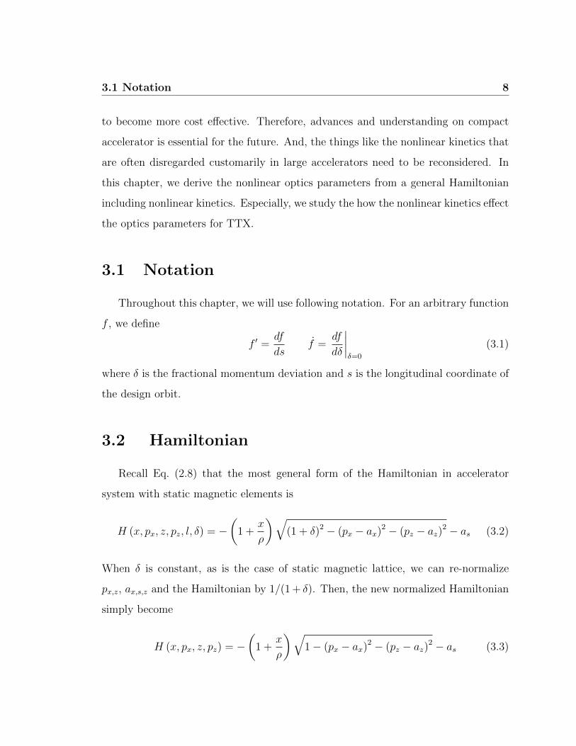
3.2 Hamiltonian
Recall Eq. (2.8) that the most general form of the Hamiltonian in accelerator
system with static magnetic elements is
H (x, px, z, pz, l, δ) = −(
1 +x
ρ
)√(1 + δ)2 − (px − ax)2 − (pz − az)2 − as (3.2)
When δ is constant, as is the case of static magnetic lattice, we can re-normalize
px,z, ax,s,z and the Hamiltonian by 1/(1 + δ). Then, the new normalized Hamiltonian
simply become
H (x, px, z, pz) = −(
1 +x
ρ
)√1− (px − ax)2 − (pz − az)2 − as (3.3)

3.2 Hamiltonian 9
The potential as can be written by
as = − x
rx(s)− z
rz(s)−Kx(s)
x2
2−Kz(s)
z2
2−Kxz(s)xz + . . . (3.4)
where rx and rz are actual field curvatures in horizontal and vertical plane respectively
while ρ is the design curvature in horizontal plane and Kx, Kz, Kxz are the focusing
strengths.
In order to get to the normal form, we first move the system onto the closed orbit.
We use the following generating function,
G = [x−∆x(s)]Px + x∆px(s) + [z −∆z(s)]Pz + z∆pz(s) (3.5)
so that
x = X + ∆x px = Px + ∆px
z = Z + ∆z pz = Pz + ∆pz (3.6)
where X, and Z are new canonical coordinate Px, and Pz are new canonical momen-
tum, ∆x and ∆z are horizontal and vertical closed orbit respectively and ∆px and ∆pz
are horizontal and vertical closed orbit momentum respectively. In general, however,
the exact solution of ∆x, ∆z, ∆px and ∆pz are not available. It has to be solved
numerically or approximately.
A good modeling, often used in accelerator physics, is to assume that the design
and actual curvature coincide for on momentum particles and thus allow the closed
orbit to arise only for off momentum particles. In this case, the closed orbit can be
calculated approximately in order of the fractional momentum deviation δ, and the
closed orbit to the first order of δ is called dispersion functions, i.e, according our

3.3 Linear optics parameter 10
notation ∆x,z.
Once we remove the closed orbit deviation, the Hamiltonian become the following
form,
H(x, px, z, pz) =∑
jklm≥2
hjklmxjzkplxp
mz (3.7)
Next, we remove horizontal and vertical linear coupling. There are infinite number
of ways to parameterize the uncoupling rotation. Typical way of doing it is described
in Ref. [7], and a sophiticated way, which is recently realized, is in Ref. [8].
After uncoupling, the Hamiltonian coefficients in Eq. (3.7) satisfy the followings
h1100 = h1001 = h0110 = h0011 = 0 (3.8)
3.3 Linear optics parameter
We start from the Eqs. (3.7,3.8) which is the linearly uncoupled Hamiltonian on
closed orbit. The linear part of the Hamiltonian looks like the following form
H = h20y2
2+ h02
p2y
2+ h11ypy (3.9)
where y is either x or z. The following generating function
G = − y2
2βy(tanφy + αy) (3.10)

3.4 Chromaticity 11
allow us to transform the linear Hamiltonian into normal form if the optics parameters
βy and αy are chosen appropriately. The new Hamiltonian reads,
H = Jy cos2 φy
(h20βy + h02
α2y
βy+αyβ
′
y
βy− 2h11αy − α
′
y
)+Jy sin2 φy
h02
βy
+Jy sinφy cosφy
(2h02
αyβy
+β
′
y
βy− 2h11
)(3.11)
Note that if the optics parameters satisfy followings
αy =2βyh11 − β
′
y
2h02
(3.12)
h02
βy= h20βy + h02
α2y
βy+αyβ
′
y
βy− 2h11αy − α
′
y (3.13)
the new Hamiltonian becomes normal form, i.e.,
H = Jyh02
βy(3.14)
Therefore, Eqs. (3.12, 3.13) defines the linear optics parameter.
3.4 Chromaticity
In addition, Eq. (3.14) tells us that the phase advance is given by
φy(s) =
∫ s
0
dsh02
βy(3.15)

3.4 Chromaticity 12
Then, the chromaticity νy can be easily calculated by
νy =
∮ds
d
dδ
(h02
2πβy
)(3.16)
Or equivalently, through Eq. (3.13),
νy =
∮ds
2π
d
dδ
(h20βy + h02
α2y
βy+αyβ
′
y
βy− 2h11αy
)(3.17)
In order to see how the nonlinear kinetics contribute to the chromaticity, we model
a storage ring with transverse magnetic elements, no linear x− z coupling, and per-
fect bending such that ax = az = 0, rx = ρ, rz = ∞ and Kxz = 0 in Eqs. (3.3,
3.4). The closed orbit is essentially dispersive in this modeling. Then, through the
canonical transformations described in the previous sections, it can be shown that
the Hamiltonian on the closed orbit become
H =1
2
(Kxx
2 +Kzz2)
+1
2
(p2x + p2
z
)+ Hδ + higher order terms
H = K2∆xx2 − z2
2+
(∆x
ρ− 1
)p2x + p2
z
2+
∆px
ρxpz (3.18)
where K2 is the sextupole strength. Therefore, according to Eq. (3.17), the chro-
maticities are
νx =1
2π
∮ [−γx
2
(1− ∆x
ρ
)+βx2K2∆x − αx
∆px
ρ
]ds (3.19)
νz =1
2π
∮ [−γz
2
(1− ∆x
ρ
)− βz
2K2∆x
]ds (3.20)
where γ = (1+α2)/β. The natural chromaticity which arise naturally due to magnetic
rigidity dependence on δ is −∮
γ4πds [11]. The last term in Eq. (3.19) corresponds

3.5 Nonlinear detuning parameters 13
to combined effect of the kinetics and curved geometry. Note that it’s effect can be
strong for small bending radius, hense for a compact ring.
3.5 Nonlinear detuning parameters
3.5.1 Canonical Perturbation
In Section 3.3, we could transform the Hamiltonian into normal form to the linear
order. The nonlinear parts need further process. In order to do this, we re-write
Eq. (3.14) including the nonlinear parts
H (φ,J ; s) = Jxh0020
βx+ Jz
h0002
βz+∑
n+m≥3
vnm (φ; s) Jn
2x J
m
2z (3.21)
Here, we are interested in normal form up to 2nd order of action so that the nonlinear
detuning parameter can be calculated. Equivalently, we want to cancel out the n +
m = 3 terms from the Hamiltonian Eq. (3.21) by a canonical transformation. To do
this, we introduce a parameterized generating function like the following and find the
solution of the parameters so that n+m = 3 terms cancel out.
G3 (φ, I; s) = φxIx + φzIz +∑
n+m=3
wnm (φ; s) In
2x I
m
2z (3.22)
Here, wnm are the parameters we want to solve. Then, the new actions are simply
I = J − ∂
∂φ
∑n+m=3
wnm (φ, s) Jn
2x J
m
2z (3.23)

3.5 Nonlinear detuning parameters 14
so that
Jn
2x J
m
2z = I
n
2x I
m
2z +
(n
2In
2−1
x Im
2z
∂
∂φx+m
2In
2x I
m
2−1
z∂
∂φz
) ∑l+k=3
wnm (φ, s) Il
2x I
k
2z (3.24)
Such a procedure is called canonical perturbation. The resulting new Hamiltonian is
H = Ixh0020
βx+ Iz
h0002
βz
+∑
n+m=3
In
2x I
m
2z
[(h0020
βx
∂
∂φx+h0002
βz
∂
∂φz+
∂
∂s
)wnm + vnm
]
+∑
n+m=3
vnm
[(n
2In
2−1
x Im
2z
∂
∂φx+m
2In
2x I
m
2−1
z∂
∂φz
) ∑l+k=3
wnm (φ, s) Il
2x I
k
2z
]+∑
n+m=4
vnmIn
2x I
m
2z + higher order terms (3.25)
The second line of Eq. (3.25) gives the equations of the generating function parameters
0 =
(h0020
βx
∂
∂φx+h0002
βz
∂
∂φz+
∂
∂s
)wnm + vnm for n+m = 3 (3.26)
In order to solve Eq. (3.26), we use Fourier decomposition.
vnm =∑σ,ρ
vσρnm(s)ei(σφx+ρφz)
wnm =∑σ,ρ
wσρnm(s)ei(σφx+ρφz) (3.27)
Then, Eq. (3.26) becomes
0 =
(iσh0020
βx+ iρ
h0002
βz+
∂
∂s
)wσρnm + vσρnm for n+m = 3 (3.28)

3.5 Nonlinear detuning parameters 15
Substituting the following ansatz [19] into Eq. (3.26)
wσρ = uσρ exp
[−i∫ds
(σh0020
βx+ ρ
h0002
βz
)](3.29)
we find that
0 =
(∂
∂suσρ)
+ vσρ exp
[i
∫ds
(σh0020
βx+ ρ
h0002
βz
)](3.30)
On the other hands, when the accelerator lattice is periodic, the Hamiltonian coeffi-
cients vnm is also periodic. Then Floquet’s theorem states that the solution of wnm
Eq. (3.26) can be factorized into periodic amplitude and a phase which increase by
same amount every periodicity. The Fourier components wσρnm are such amplitudes
which must be periodic. For a storage ring, the lattice is periodic over the circumfer-
ence C, thus according to Eq. (3.29),
uσρ(s+ C) = uσρ(s)e2πi(σνx+ρνz) (3.31)
where
2πνx ≡∫φxds =
∫h0020
βxds (3.32)
2πνz ≡∫φzds =
∫h0002
βzds (3.33)
Then, Eqs. (3.30, 3.31) lead to
uσρ(s+ C)− uσρ(s) = uσρ(s)[e2πi(σνx+ρνz) − 1
](3.34)∫ s+C
s
(∂
∂suσρ)ds = −
∫ s+C
s
ds vσρ(s)ei(σφx+ρφz) (3.35)
3.5 Nonlinear detuning parameters 16
Therefore,
wσρnm(s) =
[ie−πi(σνx+ρνz)
2 sinπ (σνx + ρνz)
∫ s+C
s
vσρei(σφx+ρφz)ds
]e−i(σφx+ρφz) (3.36)
It can be re-written in a more compact form
wσρnm(si) =i
2 sinπ (σνx + ρνz)
∮dsj v
σρnm(sj) e
i(σχxji+ρχzji) (3.37)
where
χx(z)ji ≡
φx(z)(sj)− φx(z)(si)− πνx(z) j ≥ i
φx(z)(sj)− φx(z)(si) + πνx(z) j < i
(3.38)
3.5.2 Calculation of nonlinear detuning Parameter
Once, we have removed n + m = 3 terms in Eq. (3.25), the nonlinear detuning
parameters can be easily obtained by calculation of the zeroth harmonic of the third
and fourth line of of Eq. (3.25). Let us re-write Eq. (3.25) into the following form
H (ψ, I; s) = Ixh0020
βx+ Iz
h0002
βz+ axx (ψ; s)
I2x
2+ azz (ψ; s)
I2z
2+ axz (ψ; s) IxIz + . . .
(3.39)
where the terms In
2x I
m
2z of n+m = 4 other than I2
x, I2z and IxIz are irrelevant because
they do not have zeroth harmonics when there is no resonance. Explicitly, referring
to Eq. (3.25),
axx2
= v40 +1
2v21
∂w21
∂φz+ v12
∂w30
∂φz+
3
2v30
∂w30
∂φx
axz = v22 +1
2v21
∂w03
∂φz+
1
2v12
∂w30
∂φx+ v12
∂w12
∂φz+ v21
∂w21
∂φx+
3
2v03
∂w21
∂φz+
3
2v30
∂w12
∂φxazz2
= v04 +3
2v03
∂w03
∂φz+ v21
∂w03
∂φx+
1
2v12
∂w12
∂φx(3.40)
3.5 Nonlinear detuning parameters 17
By the definition of vnm in Eq. (3.21), the harmonics vρσnm are calculated explicitly
v1030 =
√β3x
4√
2h3000 +
√βx
4√
2(i− 3αx)h2010 +
1− 2iαx + 3α3x
4√
2βxh1020
− γx
4√
2βx(αx − i)h0030
v3030 =
√β3x
12√
2h3000 −
√βx
4√
2(αx − i)h2010 +
(αx − i)2
4√
2βxh1020 −
(αx − i)3
12√
2β3x
h0030
v0121 =
γx (αz − i)2√
2βzh0021 +
αx (αz − i)√2βz
h1011 −βx
2√
2βz(αz − i)h2001 +
γx√βz
2√
2h0120
−αx√βz√
2h1110 +
βx√βz
2√
2h2100
v2121 =
(αx − i) (αz − i)2√
2βzh1011 −
(αx − i)2 (αz − i)4√
2βzβxh0021 −
βx
4√
2βz(αz − i)h2001
−√βz
2√
2(αx − i)h1110 +
(αx − i)2√βz4√
2βxh0120 +
βx√βz
4√
2h2100
v−2121 =
(αx + i) (αz − i)2√
2βzh1011 −
(αx + i)2 (αz − i)4√
2βzβxh0021 −
βx
4√
2βz(αz − i)h2001
−√βz
2√
2(αx + i)h1110 +
(αx + i)2√βz4√
2βxh0120 +
βx√βz
4√
2h2100 (3.41)
Note that these are functions of the Hamiltonian coefficient habcd and linear optics
parameter or so called twiss parameters tx(z) where t stands for β or α. Then, by
x− z symmetry
vσρnm (habcd, tx, tz) = vρσmn (hbadc, tz, tx) (3.42)
In addition, by the reality condition,
vσρnm =(v−σ,−ρmn
)∗(3.43)

3.5 Nonlinear detuning parameters 18
Therefore, Eq. (3.41) provides a complete expression of the potential harmonics vnm
for n+m = 3. As for the n+m = 4 terms, zeroth harmonic is enough.
v0040 =
γ2x
16h0040 −
αxγx4
h1030 +1 + 3α2
x
8h2020 −
αxβx4
h3010 +β2x
16h4000
v0022 = αxαzh1111 +
γxγz4h0022 +
βxβz4
h2200 −αxγz
2h1012 −
αzγx2
h0121
+βxγz
4h2002 +
βzγx4
h0220 −αzβx
2h2101 −
αxβz2
h1210 (3.44)
Again, v04 can be deduced from the x− z symmetry.
Note also that Eq. (3.40) contains terms of vjk∂wlm∂φ〈x,z〉
, where 〈x, z〉 indicate x or z.
Referring to Eqs. (3.27, 3.37), the integration on this term over the ring will result in
the following form
∮ds vjk
∂wlm∂φ〈x,z〉
= −∮ds∑σρ
i 〈σ, ρ〉 vσρjk w−σ,−ρlm
= −∮dsidsj
∑σρ
〈σ, ρ〉vσρjk(si)v
−σ,−ρlm (sj)
2 sinπ (σνx + ρνz)e−i(σχ
xji+ρχ
zji)
= −∮dsidsj
∑σρ
〈σ, ρ〉2 sinπ (σνx + ρνz)
(3.45)
×[<σρjklm cos
(σχxji + ρχzji
)+ =σρjklm sin
(σχxji + ρχzji
)]where
<σρjklm ≡ <[vσρjk(si)v
−σ,−ρlm (sj)
]= <
[v−σ,−ρjk (si)v
σρlm(sj)
]=σρjklm ≡ =
[vσρjk(si)v
−σ,−ρlm (sj)
]= −=
[v−σ,−ρjk (si)v
σρlm(sj)
](3.46)
are real and imaginary parts. Now, we are finally ready to write the nonlinear detun-
ing parameters by
αjk =
∮ds
2πajk (3.47)

3.5 Nonlinear detuning parameters 19
Explicitly,
αxx =1
π
∮ds v00
40(s)− 1
2π
∮dsjdsi
[<01
2121
cosχzjisin πνz
+ =012121
sinχzjisin πνz
]− 1
2π
∮dsjdsi
[<21
2121
cos(2χxji + χzji
)sin π (2νx + νz)
+ =212121
sin(2χxji + χzji
)sin π (2νx + νz)
]
+1
2π
∮dsjdsi
[<2,−1
2121
cos(2χxji − χzji
)sin π (2νx − νz)
+ =2,−12121
sin(2χxji − χzji
)sin π (2νx − νz)
]
− 9
2π
∮dsjdsi
[<30
3030
cos 3χxjisin 3πνx
+ =303030
sin 3χxjisin 3πνx
]− 3
2π
∮dsjdsi
[<10
3030
cosχxjisin πνx
+ =103030
sinχxjisin πνx
](3.48)
αxz =1
2π
∮ds v00
22(s)− 1
π
∮dsjdsi
[<01
2103
cosχzjisin πνz
+ =012103
sinχzjisin πνz
]− 1
π
∮dsjdsi
[<10
1230
cosχxjisin πνx
+ =101230
sinχxjisin πνx
]− 1
π
∮dsjdsi
[<12
1212
cos(χxji + 2χzji
)sin π (νx + 2νz)
+ =121212
sin(χxji + 2χzji
)sin π (νx + 2νz)
]
+1
π
∮dsjdsi
[<1,−2
1212
cos(χxji − 2χzji
)sin π (νx − 2νz)
+ =1,−21212
sin(χxji − 2χzji
)sin π (νx − 2νz)
]
− 1
π
∮dsjdsi
[<21
2121
cos(2χxji + χzji
)sin π (2νx + νz)
+ =212121
sin(2χxji + χzji
)sin π (2νx + νz)
]
− 1
π
∮dsjdsi
[<2,−1
2121
cos(2χxji − χzji
)sinπ (2νx − νz)
+ =2,−12121
sin(2χxji − χzji
)sin π (2νx − νz)
](3.49)
αzz =1
π
∮ds v00
04(s)− 1
2π
∮dsjdsi
[<10
1212
cosχxjisin πνx
+ =101212
sinχxjisin πνx
]− 1
2π
∮dsjdsi
[<12
1212
cos(χxji + 2χzji
)sin π (νx + 2νz)
+ =121212
sin(χxji + 2χzji
)sin π (νx + 2νz)
]
− 1
2π
∮dsjdsi
[<1,−2
1212
cos(χxji − 2χzji
)sinπ (νx − 2νz)
+ =1,−21212
sin(χxji − 2χzji
)sin π (2νx − 2νz)
]
− 9
2π
∮dsjdsi
[<03
0303
cos 3χzjisin 3πνz
+ =030303
sin 3χzjisin 3πνz
]− 3
2π
∮dsjdsi
[<01
0303
cosχzjisin πνz
+ =010303
sinχzjisinπνz
](3.50)

3.5 Nonlinear detuning parameters 20
3.5.3 Nonlinear detuning Parameter for a simple lattice mod-
eling
In order to grasp how the nonlinear kinetics contribute to the detuning parameter,
we use a simple lattice modeling as in Section 3.4. We assume the design curvature
coincide with actual curvature for the on momentum particle, and consider linearly
uncoupled transverse magnetic fields such that
H = −(
1 +x
ρ
)(1 + δ)
[1− p2
x + p2z
2 (1 + δ)2 −p4x + 2p2
xp2z + p4
z
8 (1 + δ)4 + . . .
]+
1
ρ
(x+
x2
2ρ
)+K1
2
(x2 − z2
)+K2
6
(x3 − 3xz2
)(3.51)
where K1, K2 and K3 are focusing, sextupole and octupole strength respectively.
This idealized modeling is approximately true for many accelerators. When there
is significant non-chromatic closed orbit deviation by fringe field, misalignment, etc,
one need to go back to general Hamiltonian Eq. (3.7). We will treat the fringe field
case in the next chapter. Plugging this model Hamiltonian into Eqs. (3.41, 3.48, 3.49,
3.50), we find that
<103030 =
K2iK2jβ3/2xi β
3/2xj
32+K2jβ
3/2xj (3α2
xi + 1)
16ρiβ1/2xi
+1 + 6α2
xi + 9α2xiα
2xj + 4αxiαxj
32ρiρjβ1/2xi β
1/2xj
=103030 = −
K2jβ3/2xj αxi
8ρiβ1/2xi
−αxi + 3αxiα
2xj
8ρiρjβ1/2xi β
1/2xj
<303030 =
K2iK2jβ3/2xi β
3/2xj
288+K2jβ
3/2xj (α2
xi − 1)
48ρiβ1/2xi
+1− 2α2
xi + α2xiα
2xj + 4αxiαxj
32ρiρjβ1/2xi β
1/2xj
=303030 = −
αxj + αxiα2xj
8ρiρjβ1/2xi β
1/2xj
−K2jβ
3/2xj αxi
24ρiβ1/2xi
(3.52)

3.5 Nonlinear detuning parameters 21
<101212 =
K2iK2jβziβzjβ1/2xi β
1/2xj
8−K2jγziβzjβ
1/2xi β
1/2xj
4ρiβzi+
β1/2xi β
1/2xj
8ρiρjβziβzj
(1 + 2α2
zi + α2ziα
2zj
)=10
1212 = 0
<121212 =
K2iK2jβziβzjβ1/2xi β
1/2xj
32+K2jβzjβ
1/2xi β
1/2xj
16ρiβzi
(1− α2
zi
)+
β1/2xi β
1/2xj
32ρiρjβziβzj
(1− 2α2
zi + α2ziα
2zj + 4αziαzj
)=12
1212 = −β
1/2xi β
1/2xj
(αzj + αziα
2zj
)8ρiρjβziβzj
+K2jαziβzjβ
1/2xi β
1/2xj
8ρiβzi
<1,−21212 = <12
1212
=1,−21212 = <12
1212 (3.53)
<101230 =
K2iK2jβ3/2xi βzjβ
1/2xj
16+γzj (1 + 3α2
xi)
16ρiρj
β1/2xj
β1/2xi
+K2iβ
2xiγzj −K2jβzj (1− 3α2
xi)
16ρi
β1/2xj
β1/2xi
=101230 = −αxi
8ρi
β1/2xj
β1/2xi
(γzjρj−K2jβzj
)(3.54)
Through these coefficients Eqs. (3.52, 3.53, 3.54), the terms which are proportional
to ρ−1 are the combined effect of the kinetics and curved geometry.
In addition, plugging the Hamiltonian coefficients of Eq. (3.51) into Eq. (3.44),
v0040 =
3
16γ2x
v0004 =
3
16γ2z
v0022 =
1
4γxγz (3.55)
we find the pure nonlinear kinetics contribution. Since γx,z ∝ β−1x,z and βx,z are gener-
ally small for compact machine, the nonlinear kinetics contribution can be important.

3.6 Numerical and Theoretical Evaluation on TTX 22
3.6 Numerical and Theoretical Evaluation on TTX
In order to demonstrate the nonlinear kinetics contribution on optics parameters,
we choose TTX[6] which is a 4.8 meter long storage ring consists 4 dipoles and 2
quadrupoles as described in Fig. 3.1 for a test bed. The specifications of elements are
listed on Table. 3.1.
Figure 3.1: Layout of TTX ring. The blue represent thequadrupoles and the red represent the dipoles[6]
3.6.1 3rd order and 4th order effect of nonlinear kinematics
In order to see how much nonlinear optics contribution come from each order of
Hamiltonian, we gradually turned on the nonlinear kinetic Hamiltonian order by order
to evaluate the theoretical values using Eqs. (3.17, 3.48, 3.49, 3.50). Table 3.2. shows
the numerical integration of the theoretical prediction for each step of the Hamiltonian
switch. The integration is performed using trapezoidal rule [22] with integration

3.6 Numerical and Theoretical Evaluation on TTX 23
Table 3.1: Specifications of elements of TTX [6]. e1, e2 are dipoleedge angles at entrance and exit. K1 is the quadrupolestrength respectively. They are chosen to produceproper tune and damping partition in absence of thefringe field correction.
Elements Specifications
Dipole l = 0.4m, θ = π/2, e1 = e2 = 0.5061Quadrupole l = 0.1m, K1 = 35m−2
Drift l = 0.5m
bin length ds = 0.001m. The natural chromaticities are indicted by the 2nd order
Hamiltonian contribution. Note that when the 3rd order of Hamiltonian terms are
turned on, the nonlinear optics parameters related to the horizontal motion increased
significantly. This is because the 3rd order terms in Hamiltonian ∼ xρ(p2x + p2
z) is
the combined effect of kinetics and geometric factor. On the other hands, the 4th
order terms in Hamiltonian ∼ (p2x+p2
z)2 contribute to the vertical detuning parameter
mostly. It can be understood by looking at Eq. (3.44) because βz is generally smaller
than βx in storage ring due to dipoles.
Table 3.2: Evaluation of theoretical chromaticity and detuning pa-rameters gradually turning on 3rd order and 4th orderHamiltonian.
Hamiltonian νx νz αxx αxz αzz
2nd -1.21 -2.16 0 0 02-3rd -2.48 -2.39 6.29 1.91 -0.0602-4th -2.48 -2.39 9.71 4.94 14.3
3.7 Conclusion 24
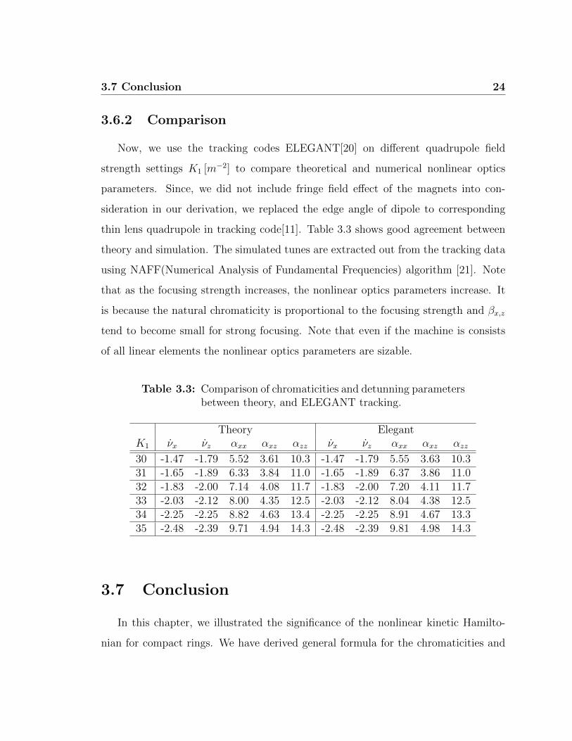
3.6.2 Comparison
Now, we use the tracking codes ELEGANT[20] on different quadrupole field
strength settings K1 [m−2] to compare theoretical and numerical nonlinear optics
parameters. Since, we did not include fringe field effect of the magnets into con-
sideration in our derivation, we replaced the edge angle of dipole to corresponding
thin lens quadrupole in tracking code[11]. Table 3.3 shows good agreement between
theory and simulation. The simulated tunes are extracted out from the tracking data
using NAFF(Numerical Analysis of Fundamental Frequencies) algorithm [21]. Note
that as the focusing strength increases, the nonlinear optics parameters increase. It
is because the natural chromaticity is proportional to the focusing strength and βx,z
tend to become small for strong focusing. Note that even if the machine is consists
of all linear elements the nonlinear optics parameters are sizable.
Table 3.3: Comparison of chromaticities and detunning parametersbetween theory, and ELEGANT tracking.
Theory ElegantK1 νx νz αxx αxz αzz νx νz αxx αxz αzz
30 -1.47 -1.79 5.52 3.61 10.3 -1.47 -1.79 5.55 3.63 10.331 -1.65 -1.89 6.33 3.84 11.0 -1.65 -1.89 6.37 3.86 11.032 -1.83 -2.00 7.14 4.08 11.7 -1.83 -2.00 7.20 4.11 11.733 -2.03 -2.12 8.00 4.35 12.5 -2.03 -2.12 8.04 4.38 12.534 -2.25 -2.25 8.82 4.63 13.4 -2.25 -2.25 8.91 4.67 13.335 -2.48 -2.39 9.71 4.94 14.3 -2.48 -2.39 9.81 4.98 14.3
3.7 Conclusion
In this chapter, we illustrated the significance of the nonlinear kinetic Hamilto-
nian for compact rings. We have derived general formula for the chromaticities and

3.7 Conclusion 25
nonlinear detuning parameters. In order to verify the formula and see the significance
of the nonlinear kinetics contribution, we tested our formula against tracking data
of a 4.8 meter long compact ring. The agreement of the theory and simulation was
beautiful. Although our formula is very general, the expression looks too long and
complicated to be useful. In addition, it is more practical to calculate the nonlinear
optics parameters using numerical particle tracking. However, the analytic expression
can still be beneficial for understanding and thus can help correction or introduction
of nonlinearities.

Dipole Fringe Field 26
Chapter 4
Dipole Fringe Field
Fringe field of dipole magnets can be important in charged-particle beam dy-
namics. Its effects on vertical focusing correction have been measured [24] and
parametrized by the fringe field integral FINT introduced by K. Brown [13]. The
nonlinear beam dynamics of fringe field has also been included up to sextupole-like
potential with hard edge approximation in Ref. [13, 17]. In recent years, compact
storage rings have been considered for the Inverse Compton Light Source [6]. As the
bending radius of dipole become small, the dipole fringe field effect become strong.
The fringe field of dipole magnets typically extends to the range of the magnet gap.
The range of fringe field is usually minimized to avoid magnetic field coupling due
to limited available space in compact storage rings. As the range of the fringe field
is reduced, i.e., the field is made to rise up or fall down sharply, the nonlinear effect
fringe field effects can be amplified. Therefore, we would like to understand how does
fringe field extent and bending radius contributes to the dipole fringe field map. Nu-
merical simulation gives much more precise fringe field map via differential algebra
of truncated power series [12]. However, analytic expression is often more useful to
understand the scaling law and thus help machine and magnet design. There already

4.1 Expected features of dipole fringe field 27
are analytic dipole fringe field mapping equations by many other authors. However,
most of them are either 3rd order map or long and very complicated form including
many double integral of fields [14, 15, 16, 13, 17]. Proper approximation without
covering important physics is necessary for good formula. Here, we present a simpler
expression with parameters of single integral, but include important physics of the
dipole fringe field effect. This work is published report. Here we give more details in
calculation steps. Better physical explanation can be found in [9]
4.1 Expected features of dipole fringe field
In order for a formula to be useful it should be able to describe the important
physics and at yet must be simple as possible. Therefore, it is important to think
about various aspects of fringe field effects, before we derive the fringe field map, so
that we know what kind of simplification and approximation is proper which does
not hide important physics and what kind of parameters we need to use or define to
describes the scaling law of the fringe field effect.
4.1.1 Closed orbit deviation
The fringe field effect on the closed orbit deviation rise from the non-constant
curvature of the particle trajectory. It can be best understood by drawing particle
a trajectory under fringe field region. We use three different curvatures ρ0 = 3ρ,
ρ1 = 2ρ and the design curvature ρ to model the fringe field for easy sketch.
First, consider a particle trajectory starting from the design orbit inside of a dipole
magnet and travels toward outside. As soon as the particle starts to see the fringe
field, which is modeled by ρ1 here, it curves less than the design curvature and result
in orbit distortion. When it fully exit out of the field region, such a orbit distortion
4.1 Expected features of dipole fringe field 28
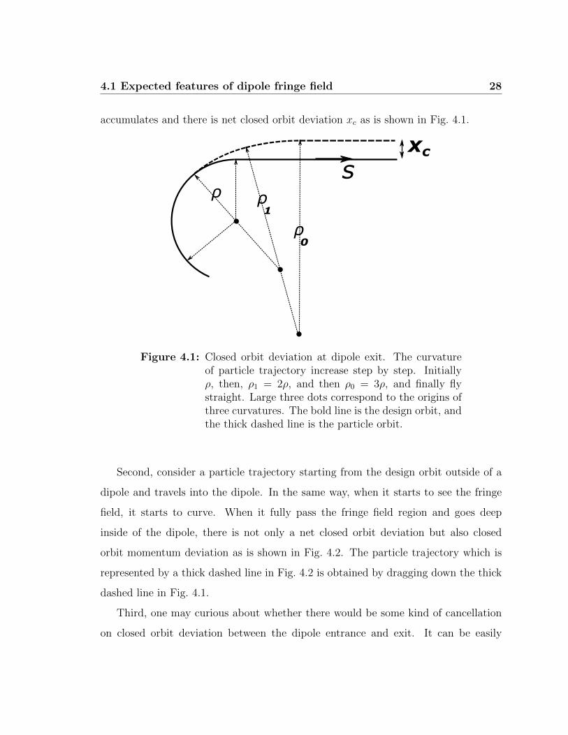
accumulates and there is net closed orbit deviation xc as is shown in Fig. 4.1.
s
xc
ρ0
ρ1
ρ
Figure 4.1: Closed orbit deviation at dipole exit. The curvatureof particle trajectory increase step by step. Initiallyρ, then, ρ1 = 2ρ, and then ρ0 = 3ρ, and finally flystraight. Large three dots correspond to the origins ofthree curvatures. The bold line is the design orbit, andthe thick dashed line is the particle orbit.
Second, consider a particle trajectory starting from the design orbit outside of a
dipole and travels into the dipole. In the same way, when it starts to see the fringe
field, it starts to curve. When it fully pass the fringe field region and goes deep
inside of the dipole, there is not only a net closed orbit deviation but also closed
orbit momentum deviation as is shown in Fig. 4.2. The particle trajectory which is
represented by a thick dashed line in Fig. 4.2 is obtained by dragging down the thick
dashed line in Fig. 4.1.
Third, one may curious about whether there would be some kind of cancellation
on closed orbit deviation between the dipole entrance and exit. It can be easily

4.1 Expected features of dipole fringe field 29
s
ρ0
ρ1
ρ
Figure 4.2: Closed orbit and momentum deviation at dipole en-trance. The curvature of particle trajectory decreasedstep by step. Initially ρ0 = 3ρ, then ρ1 = 2ρ and finallyreach ρ. Large three dots correspond to the origins ofthree curvatures. The bold line is the design orbit, andthe thick dashed line is the particle orbit. The blue linerepresent the longitudinal coordinate of Frenet-Serretframe where the the particle fully passed the fringe fieldregion. The two red lines show the angular differencebetween the design orbit and the particle orbit.
answered and understood by Fig. 4.3 where the particle enters and exit with the net
closed orbit deviation xc. Note that the closed orbit deviation is still present at both
sides.

4.1 Expected features of dipole fringe field 30
s
xc
ρ0
ρ1
ρ
xc
Figure 4.3: Illustration of presence of the closed orbit after passingthe dipole
4.1.2 Relation between fringe field extent and magnet verti-
cal gap
As we pointed out earlier, we expect the fringe field extent to play a important
role in describing fringe field effect. Using dimensional analysis, we can understand
the relationship between the vertical gap and the fringe field extent. The physical
quantities of length dimension include horizontal width, longitudinal length, and ver-
tical gap g of a dipole magnet. Among them the horizontal width and longitudinal
length are normally large enough that their effect on fringe field is minimal. There-
fore, the vertical gap is the main contribution to the fringe field extent. Apart from
the vertical gap, the pole face shaping or a magnetic clamp are used to shape the
fringe field and effectively reduce the fringe field extent. However, even after shaping
the fringe field, the extent will still increase as the vertical gap increases. The field

4.1 Expected features of dipole fringe field 31
shaping can be understood by the Enge functional model, which is often used for
fringe field modeling [12].
Bz(s)
B0
=1
1 + ec0+c1( sε)+c2( sε)2+c3( sε)
3+...
(4.1)
Here, ε is a length dimensional physical quantity relevant to the fringe field and the
coefficients ci determines field shape and can effectively reduce the fringe field extent.
This modeling is quite general because we can include as many of ci as needed to fit to
the actual field shape. Note, however, that ε still plays the major role in determining
the fringe field extent. Since, the only relevant length dimensional quantity is the
vertical gap, we identify ε = g
4.1.3 Horizontal field degradation
It is expected that the field is strongest at the center of the horizontal dimension
of the magnet and become weaker toward each horizontal ends of the magnet. This
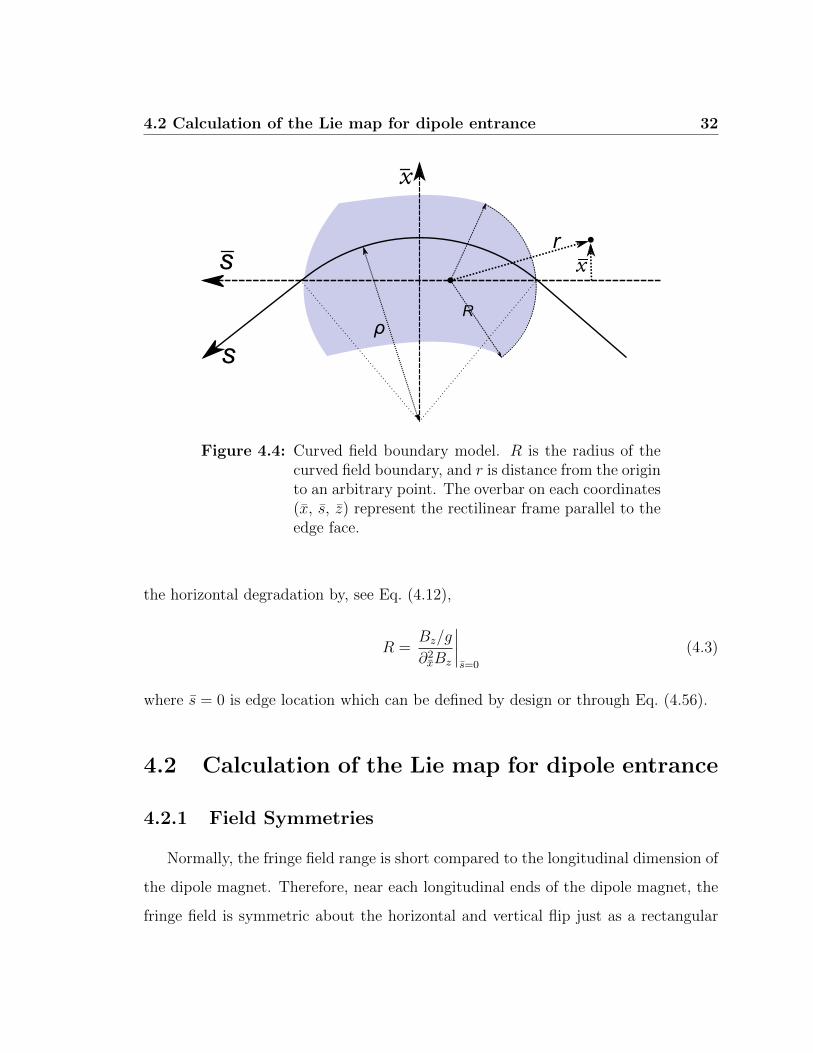
fact can be modeled by the curved field boundary introduced by K. Brown [13] as
shown in Fig. 4.4 where the shaded region indicate the field contour. The boundary
does not indicate strict hard edge, rather it represent an equipotential line. Note that
the relevant parameter that describes the horizontal field degradation is the curvature
R of the edge. Under this modeling the magnetic scalar potential can be written by
Φ (r, z)
Bρ=∑n=0
ψ2n+1 (r)z2n+1
(2n+ 1)!(4.2)
However, we will not restrict our formula to be dependent on such a modeling. What
learned from this modeling is that we can define a relevant quantity R to describes
4.2 Calculation of the Lie map for dipole entrance 32
s
s
x
R
r
x
ρ
Figure 4.4: Curved field boundary model. R is the radius of thecurved field boundary, and r is distance from the originto an arbitrary point. The overbar on each coordinates(x, s, z) represent the rectilinear frame parallel to theedge face.
the horizontal degradation by, see Eq. (4.12),
R =Bz/g
∂2xBz
∣∣∣∣s=0
(4.3)
where s = 0 is edge location which can be defined by design or through Eq. (4.56).
4.2 Calculation of the Lie map for dipole entrance
4.2.1 Field Symmetries
Normally, the fringe field range is short compared to the longitudinal dimension of
the dipole magnet. Therefore, near each longitudinal ends of the dipole magnet, the
fringe field is symmetric about the horizontal and vertical flip just as a rectangular

4.2 Calculation of the Lie map for dipole entrance 33
dipole magnet does. This is illustrated in Figure 4.5 of a rectangular dipole magnet.
s
xx
s
xx
ρ
x
θEθS
Figure 4.5: The rectilinear frame (rFrame) coordinate system vsthe Frenet-Serret frame (fsFrame) coordinate system.The rFrame is characterized by adding bar on top ofeach variable. The shaded region indicate the dipole.ρ is the design curvature, θE is the edge angle, θE − θSis the rotation angle of design orbit, s is the longitu-dinal coordinate in the fsFrame and s is the longitudi-nal coordinate in the rFrame. The drawing is about arectangular dipole for easy understanding, but the co-ordinate relation can be used for any edge angle. Also,the horizontal and vertical mirror symmetry applies forany edge angle near the longitudinal ends of the dipole.
Referring to the Figure 4.5, we find that relation between the rectilinear frame
and the Frenet-Serret frame near the entrance is,
s (x, s) = ρ(s) sin θE − (ρ+ x) sin θS (4.4)
x (x, s) = (ρ(s) + x) cos θS − ρ(s) cos θE (4.5)
where, ρ is constant inside of dipole and become ρ(s < 0) =∞ before dipole entrance,

4.2 Calculation of the Lie map for dipole entrance 34
and
θS = θE −s
ρ(s)(4.6)
Then, the magnetic scalar potential can be written as
Φ (x, s, z)
Bρ=
∑n,m=0
φ2m,2n+1 (s)x2m
(2m)!
z2n+1
(2n+ 1)!(4.7)
where Bρ is the particle rigidity under magnetic field. Remember that φ01 is order
of 1/ρ. Using the Poisson equation, we find
0 = φ′′
2m,2n+1 + φ2m+2,2n+1 + φ2m,2n+3 (4.8)
where the prime indicate the differentiation by s. Therefore, we find the magnetic
potential up to 4th order of coordinate variable is,
Φ
Bρ' φ01z + φ21
x2
2z −
(φ
′′
01 + φ21
) z3
3!. (4.9)
On the other hand, the expansion of Eq. (4.2) in order of x is
Φ
Bρ' ψ1z +
∂rψ1
R− sx2
2z + ψ3
z3
3!(4.10)
which gives, compared to Eq. (4.9)
φ01 = ψ1 (4.11)
φ21 =∂rψ1
R− s(4.12)
The 2nd equation tells us the order of magnitude of φ21 and suggest to define R as
in Eq. (4.3).

4.2 Calculation of the Lie map for dipole entrance 35
4.2.2 Vector Potential
So far, we have constructed magnetic potential in rectilinear frame(rFrame). In
order to construct Hamiltonian for Frenet-Serret frame(fsFrame), we would like to
build the vector potential in fsFrame. As the vector potential is not unique, we fix
the gauge such that Az = 0. Then, B = −∇Φ = ∇× A simplifies to
−hs∂Φ
∂x= −∂As
∂z(4.13)
− 1
hs
∂Φ
∂s=
∂Ax∂z
(4.14)
−hs∂Φ
∂z=
∂As∂x− ∂Ax
∂s(4.15)
where hs = 1 + x/ρ(s) is the geometric factor. The Eq. (4.13) and Eq. (4.14) give us
As =
∫dz
[hs∂Φ
∂x
]+ f (x, s) (4.16)
Ax = −∫dz
[1
hs
∂Φ
∂s
]+ g (x, s) (4.17)
where f and g are arbitrary functions which comes from remaining gauge freedom.
Then Eq. (4.15) become
−hs∂Φ
∂z=
∫dz
[∂
∂xhs∂Φ
∂x+
∂
∂s
1
hs
∂Φ
∂s
]+
∂
∂xf (x, s)− ∂
∂sg (x, s)
=
∫dz
[hs∇2Φ− ∂
∂zhs∂Φ
∂z
]+
∂
∂xf (x, s)− ∂
∂sg (x, s)
= −hs∂Φ
∂z+
[hs∂Φ
∂z
]z=0
+∂
∂xf (x, s)− ∂
∂sg (x, s) (4.18)
If we fix g = 0, which is still allowed by gauge freedom because g does not depends
on z, we find
f (x, s) = −∫dx
[hs∂Φ
∂z
]z=0
, (4.19)
4.2 Calculation of the Lie map for dipole entrance 36
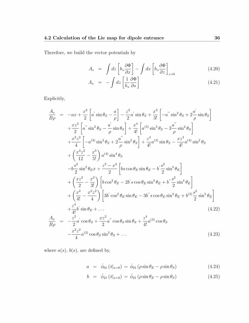
Therefore, we build the vector potentials by
As =
∫dz
[hs∂Φ
∂x
]−∫dx
[hs∂Φ
∂z
]z=0
(4.20)
Ax = −∫dz
[1
hs
∂Φ
∂s
](4.21)
Explicitly,
AsBρ
= −ax+x2
2
[a
′sin θS −
a
ρ
]− z2
2a
′sin θS +
x3
3!
[−a′′
sin2 θS + 2a
′
ρsin θS
]+xz2
2
[a
′′sin2 θS −
a′
ρsin θS
]+x4
4!
[a(3) sin3 θS − 3
a′′
ρsin2 θS
]+x2z2
4
[−a(3) sin3 θS + 2
a′′
ρsin2 θS
]+z4
4!a(3) sin θS −
xz4
4!a(4) sin2 θS
+
(x3z2
12− x5
5!
)a(4) sin4 θS
−bs2
2sin2 θEx+
z2 − x2
2
[bs cos θE sin θE − b
′ s2
2sin3 θE
]+
(xz2
2− x3
3!
)[b cos2 θE − 2b
′s cos θE sin2 θE + b
′′ s2
2sin4 θE
]+
(x4
4!− x2z2
4
)[3b
′cos2 θE sin θE − 3b
′′s cos θE sin3 θE + b(3) s
2
2sin5 θE
]+z4
4!b′sin θE + . . . (4.22)
AxBρ
= −z2
2a
′cos θS +
xz2
2a
′′cos θS sin θS +
z4
4!a(3) cos θS
−x2z2
4a(3) cos θS sin2 θS + . . . (4.23)
where a(s), b(s), are defined by,
a = φ01 (s|x=0) = φ01 (ρ sin θE − ρ sin θS) (4.24)
b = φ21 (s|x=0) = φ21 (ρ sin θE − ρ sin θS) (4.25)

4.2 Calculation of the Lie map for dipole entrance 37
4.2.3 Fringe Field Hamiltonian
The Hamiltonian can be obtained by
HF = HF (x, px, z, pz) (4.26)
= −(
1 +x
ρ
)√(1 + δ)2 −
(px −
AxBρ
)2
− pz −AsBρ
where δ is the fractional momentum deviation. We confine our effective thin map up
to 4th order of canonical variables which are responsible to nonlinear detuning. In
order for this, we write the Hamiltonian up to 5-th order of canonical variables if it
contains x or px, otherwise up to 4-th order, because there is a closed orbit deviation
in horizontal direction.
HF ' D + x
[a− 1 + δ
ρ
]+z2
2
[a′ sin θS + a′
cos θS1 + δ
px
]+x2
2
[a
ρ− a′ sin θS
]+x3
3!
[a
′′sin2 θS − 2
a′
ρsin θS
]+xz2
2
[a
′
ρsin θS − a
′′sin2 θS
] [1 +
px1 + δ
cot θS
]+x4
4!
[3a
′′
ρsin2 θS − a(3) sin3 θS
]+x2z2
4
[a(3) sin3 θS − 2
a′′
ρsin2 θS
] [1 +
px1 + δ
cot θS
]+z4
4!
[−a(3) sin θS
(1 +
px1 + δ
cot θS
)+ 3
(a
′)2 cos2 θS1 + δ
]+
[x5
5!− x3z2
3!2!
] [a(4) sin4 θS
]+xz4
4!
[a(4) sin2 θS
]−x[bs2
2sin2 θE
]+x2 − z2
2
[bs cos θE sin θE − b
′ s2
2sin3 θE
]+
[x3
3!− xz2
2
] [b cos2 θE − 2b′s cos θE sin2 θE + b′′
s2
2sin4 θE
](4.27)

4.2 Calculation of the Lie map for dipole entrance 38
where we have included 5-th order terms, and
D =p2x + p2
z
2(1 + δ)(4.28)
By dimensional analysis, it can be shown that the leading order of each n-th order
multipole potential in effective thin map is order of g2−n. Here, we have kept the
terms up which will retain the effective thin map to the next leading order for each
multipole potential. We will make this statement clearer after few subsection.
4.2.4 Magnus’s exponential solution
In order to calculate the map, we would like to briefly introduce some of the Lie
algebraic technique. Let H be the time evolution operator from s0 to s which act on
canonical variables of Hamiltonian system such that x(s) = H (x(s0), s)x(s0), where
x is the set of canonical variables and s is the time variable. Then it satisfies following
differential equation [25].
d
dsx(s) = − :H (x(s); s): x(s)
= −H :H (x(s0); s): H−1Hx(s0) (4.29)
where H is the Hamiltonian and the pair of colons is the Dragt’s notation [25] of
the Poisson bracket such that : f : g = [f, g]. The direct differentiation of the time
evolution operator givesd
dsx(s) =
(d
dsH)x(s0) (4.30)
Comparing Eq. (4.2.4) and Eq. (4.30), we find,
d
dsH (x(s0), s) = −H (x(s0), s) :H (x(s0), s): (4.31)
4.2 Calculation of the Lie map for dipole entrance 39
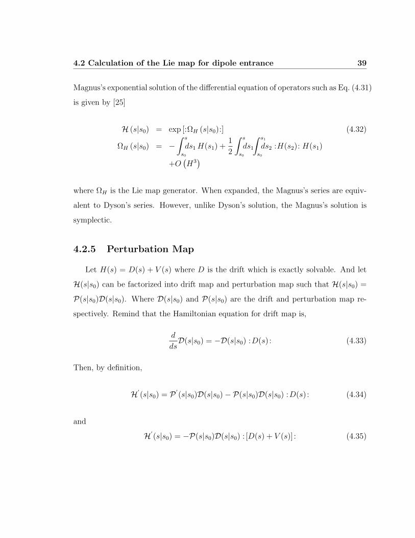
Magnus’s exponential solution of the differential equation of operators such as Eq. (4.31)
is given by [25]
H (s|s0) = exp [:ΩH (s|s0):] (4.32)
ΩH (s|s0) = −∫ s
s0
ds1H(s1) +1
2
∫ s
s0
ds1
∫ s1
s0
ds2 :H(s2): H(s1)
+O(H3)
where ΩH is the Lie map generator. When expanded, the Magnus’s series are equiv-
alent to Dyson’s series. However, unlike Dyson’s solution, the Magnus’s solution is
symplectic.
4.2.5 Perturbation Map
Let H(s) = D(s) + V (s) where D is the drift which is exactly solvable. And let
H(s|s0) can be factorized into drift map and perturbation map such that H(s|s0) =
P(s|s0)D(s|s0). Where D(s|s0) and P(s|s0) are the drift and perturbation map re-
spectively. Remind that the Hamiltonian equation for drift map is,
d
dsD(s|s0) = −D(s|s0) :D(s) : (4.33)
Then, by definition,
H′(s|s0) = P ′
(s|s0)D(s|s0)− P(s|s0)D(s|s0) :D(s) : (4.34)
and
H′(s|s0) = −P(s|s0)D(s|s0) : [D(s) + V (s)] : (4.35)

4.2 Calculation of the Lie map for dipole entrance 40
Therefore,
P ′(s|s0) = −P(s|s0)D(s|s0) :V (s) : D−1(s|s0)
= −P(s|s0) :D(s|s0)V (s) : (4.36)
Which is exactly same form as Eq. (4.31). Thus, by analogy,
P (s|s0) = exp [:ΩV (s|s0):] (4.37)
ΩV (s|s0) = −∫ s
s0
ds1 :D (s1|s0)V (s1) +1
2
∫ s
s0
ds1
∫ s1
s0
ds2
× ::D (s2|s0)V (s2): D (s1|s0)V (s1):
From the first order of Magnus’s Series, it can be easily shown that the Lie map for
a piece wise constant accelerator element of the length li is exp(− : Hili :) where
Hi is the corresponding Hamiltonian of that element. Therefore, the exponent of
the Magnus’s solution corresponds to the effective thin Hamiltonian multiplied by
arbitrary length dimension.
4.2.6 Thin Map
What we are interested is the effective thin map. It can be obtained by sandwich-
ing with inverse drift and inverse ideal bending map. In order to keep track of the
leading order and next leading order for the calculation of the effective thin map, it is
convenient to separate the potential into terms with order of ρ−1 and ρ−2 or ρ−1R−1,
such that
HF = D + VF +WF (4.38)
HB = D + VB +WB (4.39)

4.2 Calculation of the Lie map for dipole entrance 41
where HF and HB are fringe field and ideal(hard edge) bending magnet Hamilto-
nian respectively. And V and W are potentials order of O(ρ−1) and O(ρ−2, ρ−1R−1)
respectively.
Let D, F , and B be the time evolution operators generated by D, HF and HB
respectively. Using Eq. (4.37), these operators become
F(L| − L) = exp [:ΩF :]D(L| − L) (4.40)
B(L|0) = exp [:ΩB :]D(L|0), (4.41)
where L ∼ O(g) is an integration length which must large enough to cover the fringe
field region. Then, the effective thin map M of the dipole entrance becomes
M = D−1(0| − L)F(L| − L)B−1(L|0)
= exp[:D−1(0| − L)ΩF :
]exp [− :ΩB :]
= exp
[:D−1(0| − L)ΩF : − :ΩB : −1
2::D−1(0| − L)ΩF : ΩB : + . . .
]≡ exp [:ΩM :] , (4.42)
where we have used Baker-Campbell-Hausdorff formula [25]. Defining the interaction
picture potential by
V int(s) = D(s|0)V (s) (4.43)
W int(s) = D(s|0)W (s), (4.44)

4.2 Calculation of the Lie map for dipole entrance 42
the exponent of M becomes
ΩM = −∫ L
−Lds1 V
intF (s1)−
∫ L
−Lds1W
intF +
∫ L
−0
ds1 VintB (s1) +
∫ L
−0
ds1WintB
+1
2
∫ L
−Lds1
∫ s1
−Lds2 :V int
F (s2): V intF (s1)− 1
2
∫ L
0
ds1
∫ s1
0
ds2 :V intB (s2): V int
B (s1)
−1
2
∫ L
−Lds2
∫ L
0
ds1 :V intF (s2): V int
B (s1). (4.45)
4.2.7 Leading Order and Next Leading Order
Recall that we wrote earlier that we will retain the effective thin Hamiltonian to
the next leading order for each multipole potential. Throughout previous subsections
on Lie map, we are finally ready to make this statement clear. By effective thin
Hamiltonian, we mean ΩM in Eq. (4.45). It can be put into the following form.
ΩM =∑n,m
Cnmqnpm (4.46)
where q represent x or z and p represent px or pz. Recall that the relevant length
dimensional quantities responsible for fringe field description are ρ, R, and g. It
is generally true that g ρ and g R. And the fringe field thin map must be
at least order of O(ρ−1) because it must be depends on field strength. Then, since
the ΩM is dimension of length, the leading order of C10 and C20, for example, are
O (ρ−1g) and O (ρ−1) respectively. Therefore, leading order of each k-th multipole
which corresponds to Cnm with n + m = k is O(g2−k). Same way, the next leading
order of each k-th multipole is O(g3−k). Note that the dimensional analysis says
that the leading order of sextupole and octupole-like potential are O(g−1ρ−1) and
O(g−2ρ−1) respectively. However, since these order of terms are linear in the field
strength, they will averaged out when integrated. This is one of the reason why hard

4.2 Calculation of the Lie map for dipole entrance 43
edge approximation fail to describe the octupole-like potential in many literature.
Therefore, the next leading order from the dimensional analysis become actual leading
order for the nonlinear terms.
4.2.8 Integrands
In order to calculate the integrands of Eq. (4.45), we first calculate the interaction
picture potential. Plugging the drift map
D(s|0)x = x+px
1 + δs (4.47)
D(s|0)z = z +pz
1 + δs, (4.48)

4.2 Calculation of the Lie map for dipole entrance 44
we obtain,
V intF =
[x+
px1 + δ
s
] [a− 1 + δ
ρ
]+
[z2
2+ z
pz1 + δ
s− x2
2− x px
1 + δs
][a′ sin θS]
+z2
2
px1 + δ
[a′ cos θS]− xz2
2
px1 + δ
[a
′′sin θS cos θS
]+
[x3
3!+x2
2
px1 + δ
s− xz2
2− z2
2
px1 + δ
s− xz pz1 + δ
s
] [a
′′sin2 θS
]+
[x2z2
4+xz2
2
px1 + δ
s+x2z
2
pz1 + δ
s− x4
4!− x3
3!
px1 + δ
s
] [a(3) sin3 θS
]−[z4
4!+z3
3!
pz1 + δ
s
] [a(3) sin θS
]+x2z2
4
px1 + δ
[a(3) sin2 θS cos θS
]−z
4
4!
px1 + δ
[a(3) cos θS
]+
[xz4
4!+z4
4!
px1 + δ
s+xz3
3!
pz1 + δ
s
] [a(4) sin2 θS
]+
[x5
5!− x3z2
3!2!+x4
4!
px1 + δ
s− x2z2
4
px1 + δ
s− x3z
3!
pz1 + δ
s
] [a(4) sin4 θS
]W intF =
a
ρ
x2
2+
[xz2
2− x3
3
] [a
′
ρsin θS
]+
[x4
8− x2z2
2
] [a
′′
ρsin2 θS
]+z4
8
[(a
′)2 cos2 θS1 + δ
]−x[bs2
2sin2 θE
]+x2 − z2
2
[bs cos θE sin θE − b
′ s2
2sin3 θE
]+
[x3
3!− xz2
2
] [b cos2 θE − 2b′s cos θE sin2 θE + b′′
s2
2sin4 θE
](4.49)

4.2 Calculation of the Lie map for dipole entrance 45
Second, we perform Poisson bracket to obtain other integrands of Eq. (4.45)
:V intF (s2):V int
F (s1) = x
[a
′
1
ρ2
− a2a′
1
1 + δ+ (1↔ 2)
](s1 − s2) sin θE
+x2
2
[a
′
2a′
1
1 + δ+a2a
′′
1
1 + δ− a
′′
1
ρ2
+ (1↔ 2)
](s1 − s2) sin2 θE
+z2
2
[a
′
2a′
1
1 + δ− a2a
′′
1
1 + δ+a
′′
1
ρ2
+ (1↔ 2)
](s1 − s2) sin2 θE
+z2
2
[a2a
′
1
1 + δ− a
′
1
ρ2
− (1↔ 2)
]cos θE
+x3
3!
[−3
a′
2a′′
1
1 + δ− a2a
(3)1
1 + δ+a
(3)1
ρ2
+ (1↔ 2)
](s1 − s2) sin3 θE
+xz2
2
[− a
′
2a′′
1
1 + δ+a2a
(3)1
1 + δ− a
(3)1
ρ2
+ (1↔ 2)
](s1 − s2) sin3 θE
+xz2
2
[− a2a
′′
1
1 + δ+a
′′
1
ρ2
− (1↔ 2)
]cos θE sin θE
+x4
4!
[3a
′′
2a′′
1
1 + δ+ 4
a′
2a(3)1
1 + δ+a2a
(4)1
1 + δ− a
(4)1
ρ2
+ (1↔ 2)
](s1 − s2) sin4 θE
+x2z2
4
[a
′′
2a′′
1
1 + δ− a2a
(4)1
1 + δ+a
(4)1
ρ2
+ (1↔ 2)
](s1 − s2) sin4 θE
+x2z2
4
[a
′
2a′′
1
1 + δ+a2a
(3)1
1 + δ− a
(3)1
ρ2
− (1↔ 2)
]cos θE sin2 θE
+z4
4!
[6a
′′
2a′′
1
1 + δ
](s1 − s2) sin4 θE
+z4
4!
[6a
′
2a′′
1
1 + δ− (1↔ 2)
]cos θE sin2 θE
+z4
4!
[−4
a′
2a(3)1
1 + δ+a2a
(4)1
1 + δ− a
(4)1
ρ2
+ (1↔ 2)
](s1 − s2) sin2 θE
+z4
4!
[−a2a
(3)1
1 + δ+a
(3)1
ρ2
− (1↔ 2)
]cos θE (4.50)

4.2 Calculation of the Lie map for dipole entrance 46
where (1↔ 2) indicates terms with exchanged indices 1 and 2. For example, the first
line is
[a
′
1
ρ2
− a2a′
1
1 + δ+ (1↔ 2)
](s1 − s2) =
[a
′
1
ρ2
− a2a′
1
1 + δ+a
′
2
ρ1
− a1a′
2
1 + δ
](s1 − s2)
4.2.9 Integration
The integration in Eq. (4.45) are over the longitudinal time variable s of the design
orbit. However measuring real field following the curved frame can be cumbersome.
It would be easier to measure field on the rectilinear frame. Therefore, we would like
to convert the integration variable from s to s. Using Eqs. (4.4, 4.5), we find
ds =ds
cos θS' ds
cos θE
(1− s
ρ
sin θEcos2 θE
)s ' s
cos θE− s2
2ρ
sin θEcos3 θE
As we mentioned in earlier sections the integration range L must also be large enough
to cover the fringe field region. Therefore, the following boundary condition holds
a(L) = 1/ρ a(−L) = 0 a(n)(±L) = 0
b(±L) = 0 b(n)(±L) = 0 (4.51)
where the superscript in the parenthesis (n) indicates n-th order derivative.
Then, we obtain following integration
∫ L
−Lds1 a1 =
I (a)
cos θE− sin θEρ cos3 θE
J (as)∫ L
−Lds1
1
ρ1
=L/ρ
cos θE− L2 sin θE
2ρ2 cos3 θE

4.2 Calculation of the Lie map for dipole entrance 47
∫ L
−Lds1
s1
ρ1
=L2/2
ρ cos2 θE∫ L
−Lds1 a
′
1s1 =L
ρ cos2 θE− I (a)
cos2 θE∫ L
−Lds1 a
′
1 sin θ1 =tan θEρ− 1
ρ cos3 θE
(L
ρ− J (a)
)∫ L
−Lds1 a
′′
1 sin2 θ1 =1
ρ
(sin3 θEcos3 θE
+ 2sin θEcos θE
)(1
ρ− a(0)
)∫ L
−Lds1 a
(3)1 sin3 θ1 = −1
ρ
(sin4 θEcos3 θE
+ 3sin2 θEcos θE
)a
′(0)∫ L
−Lds1 a
(3)1 sin θ1 = − a
′(0)
ρ cos3 θE
And,
∫ L
−Lds1
∫ s1
−Lds2
(a2a
′
1 + a′
2a1
)(s1 − s2) =
LI (a)− I (as)
ρ cos3 θE∫ L
−Lds1
∫ s1
−Lds2
(a
′
1
ρ2
+a
′
2
ρ1
)(s1 − s2) =
1
cos3 θE
(L
ρI (a) +
L2
2ρ2− 2
J (as)
ρ
)∫ L
−Lds1
∫ s1
−Lds2
(a
′
1
ρ2
− a′
2
ρ1
)=
1
cos2 θE
(L
ρ2− 2
J (a)
ρ
)∫ L
−Lds1
∫ s1
−Lds2
(a2a
′
1 − a1a′
2
)=
1
cos2 θE
(I (a)
ρ− 2I
(a2))
∫ L
−Lds1
∫ s1
−Lds2
(a
′′
1
ρ2
+a
′′
2
ρ1
)(s1 − s2) =
1
cos3 θE
(2J (a)
ρ− L
ρ2
)∫ L
−Lds1
∫ s1
−Lds2
(a2a
′′
1 + a′′
2a1
)(s1 − s2) =
1
cos3 θE
(2I(a2)− I (a)
ρ
)∫ L
−Lds1
∫ s1
−Lds2 a
′
2a′
1 (s1 − s2) =1
cos3 θE
(I (a)
ρ− I
(a2))
∫ L
−Lds1
∫ s1
−Lds2 a
′
2a′
1 =1
2ρ2 cos2 θE∫ L
−Lds1
∫ s1
−Lds2
(a2a
′′
1 − a′′
2a1
)= − 1
ρ2 cos3 θE
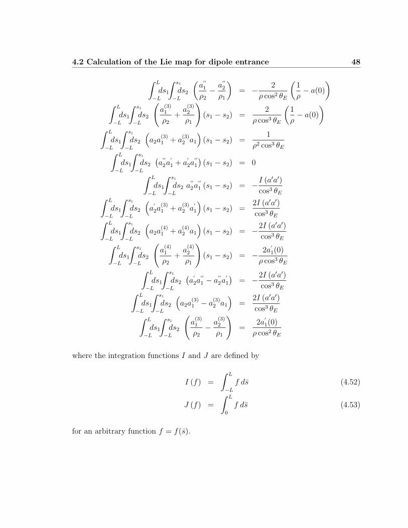
4.2 Calculation of the Lie map for dipole entrance 48
∫ L
−Lds1
∫ s1
−Lds2
(a
′′
1
ρ2
− a′′
2
ρ1
)= − 2
ρ cos2 θE
(1
ρ− a(0)
)∫ L
−Lds1
∫ s1
−Lds2
(a
(3)1
ρ2
+a
(3)2
ρ1
)(s1 − s2) =
2
ρ cos3 θE
(1
ρ− a(0)
)∫ L
−Lds1
∫ s1
−Lds2
(a2a
(3)1 + a
(3)2 a1
)(s1 − s2) =
1
ρ2 cos3 θE∫ L
−Lds1
∫ s1
−Lds2
(a
′′
2a′
1 + a′
2a′′
1
)(s1 − s2) = 0∫ L
−Lds1
∫ s1
−Lds2 a
′′
2a′′
1 (s1 − s2) = −I (a′a′)
cos3 θE∫ L
−Lds1
∫ s1
−Lds2
(a
′
2a(3)1 + a
(3)2 a
′
1
)(s1 − s2) =
2I (a′a′)
cos3 θE∫ L
−Lds1
∫ s1
−Lds2
(a2a
(4)1 + a
(4)2 a1
)(s1 − s2) = −2I (a′a′)
cos3 θE∫ L
−Lds1
∫ s1
−Lds2
(a
(4)1
ρ2
+a
(4)2
ρ1
)(s1 − s2) = − 2a
′
1(0)
ρ cos3 θE∫ L
−Lds1
∫ s1
−Lds2
(a
′
2a′′
1 − a′′
2a′
1
)= −2I (a′a′)
cos3 θE∫ L
−Lds1
∫ s1
−Lds2
(a2a
(3)1 − a
(3)2 a1
)=
2I (a′a′)
cos3 θE∫ L
−Lds1
∫ s1
−Lds2
(a
(3)1
ρ2
− a(3)2
ρ1
)=
2a′
1(0)
ρ cos2 θE
where the integration functions I and J are defined by
I (f) =
∫ L
−Lf ds (4.52)
J (f) =
∫ L
0
f ds (4.53)
for an arbitrary function f = f(s).

4.2 Calculation of the Lie map for dipole entrance 49
4.2.10 Lie Map Generator I
Putting all the integration we calculated, we finally obtain the Lie map generator
ΩM =x
cos θE
[L
ρ− I (a)
]− xsec3 θE sin θE
2ρ (1 + δ)
[L2
2ρ− I (as)
]+
px(1 + δ) cos2 θE
[L2
2ρ− I (as)
]+xpx − zpz
1 + δ
[L
ρ− I (a)
]sin θEcos2 θE
+x2 − z2
2
tan θEρ− x2
2
sin2 θE2ρ (1 + δ) cos3 θE
[L
ρ− I (a)
]+z2
2
sec3 θE(1 + δ)
[L
2ρ2+I (a)
2ρ− I
(a2)]
+z2
2
sin2 θE(1 + δ) cos3 θE
[I (a)
ρ− I
(a2)]
−x3
3!
tan3 θE2ρ2 (1 + δ)
+xz2
2
[tan θE sec2 θE
2ρ2 (1 + δ)
]− z2px
2ρ (1 + δ)
+
[x2px − z2px − 2xzpz
2 (1 + δ)
]tan2 θEρ
+z4
4!
[4
cos θE− 8
cos3 θE
]I(a′2)
+xsin2 θE
2 cos3 θEI(bs)
+z2 − x2
2
sin θEcos3 θE
I(bs)
+
[xz2
2− x3
3!
]I(b)
cos3 θE(4.54)
Note that the Lie map generator we calculated has explicit dependence on L. This
is not well defined. To be mathematically strict, L must be sent to infinity because
L should cover all the fringe field region. There, we have to combine L dependence
terms with field integration. In the following subsection, we define field integration
parameters which do this job.

4.2 Calculation of the Lie map for dipole entrance 50
4.2.11 Field Integration
Here, we define field integration parameters as followings
K0 =
∫ ∞−∞
B0Θ (s) s−Bz s
B0g2ds (4.55)
K1 =
∫ ∞−∞
B0Θ (s)−Bz
B0gds (4.56)
K2 =
∫ ∞−∞
Bz (B0 −Bz)
B20g
ds (4.57)
K3 = g
∫ ∞−∞
B′
zB′
z
B20
ds (4.58)
K4 =R
g2
∫ ∞−∞
∂2xBz s
2
B0
ds (4.59)
K5 =R
g
∫ ∞−∞
∂2xBz s
B0
ds (4.60)
K6 = R
∫ ∞−∞
∂2xBz
B0
ds (4.61)
where Θ (s) is the Heaviside step function which is zero when s < 0 and one when
s ≥ 0, and B0 = 1/ρ is design field strength, Bz is the s dependent vertical B-field
at x = z = 0, and ∂x is derivative with respect to x. The normalization quantities g,
and R are multiplied to make the field integration parameters not only dimensionless
but also universal. It means the value does not vary significantly over many different
dipole magnets. For example, consider K3. The relevant dimensional contributions
come from ds and d/ds which are order of g and g−1 respectively. By multiplying
the normalization constant g, the definition of K3 become order of unity and thus
universal. This is the same way K. Brown defined the field integral so called FINT
to describe the focusing correction term [13]. Here K2 is exactly same with FINT.

4.3 Calculation of the Lie map for dipole exit 51
4.2.12 Lie Map Generator II
Using the defined field integration parameters Eqs. (4.55-4.61), the Lie map gen-
erator Eq. (4.54) can be re-written by
ΩM =x
cos θE
g
ρK1 − x
sec3 θE sin θE2 (1 + δ)
g2
ρ2K0 + px
sec2 θE(1 + δ)
g2
ρK0 +
xpx − zpz1 + δ
g
ρK1
sin θEcos2 θE
+x2 − z2
2
tan θEρ− x2
2
sin2 θE2ρ (1 + δ) cos3 θE
g
ρK1 +
z2
2
sec3 θE(1 + δ)
[g
2ρ2K1 +
g
ρ2K2
]+z2
2
sin2 θE(1 + δ) cos3 θE
g
ρ2K2 −
x3
3!
tan3 θE2ρ2 (1 + δ)
+xz2
2
[tan θE sec2 θE
2ρ2 (1 + δ)
]+
[x2px − z2px − 2xzpz
2 (1 + δ)
]tan2 θEρ
− z2px2ρ (1 + δ)
+z4
4!
[4
cos θE− 8
cos3 θE
]K3
ρ2g
+xsin2 θE
2 cos3 θE
g2
ρRK4 +
z2 − x2
2
sin θEcos3 θE
g
ρRK5 +
[xz2
2− x3
3!
]K6/ρR
cos3 θE(4.62)
Note that the normalization factors of the field integration parameters in Eqs. (4.55-
4.61) cancel with coefficients of Eq. (4.62). However, it does not mean that the
scaling law shown explicitly in Eq. (4.62), does not holds. Rather, recall that the
field integration parameters are normalized so that they are order of unity.
4.3 Calculation of the Lie map for dipole exit
The effective thin map for dipole exit can be calculated in the same way. However,
it is not that trivial task to obtain it out of Eq. (4.62).

4.3 Calculation of the Lie map for dipole exit 52
4.3.1 Fringe field Hamiltonian
Near the exit of the Dipole, Eq. (4.4) and Eq. (4.5) modifies to
s (x, s) = −ρ(s) sin θE + (ρ+ x) sin θS (4.63)
x (x, s) = (ρ(s) + x) cos θS − ρ(s) cos θE (4.64)
where s = 0 is now the location of edge of the dipole exit. θs also modifies to,
θS ≡ θE +s
ρ(4.65)
Note that Eq. (4.63) and Eq. (4.64) become identical to Eq. (4.4) and Eq. (4.5) if the
sign of θE and θS are flipped. Since the edge angle effect on the entrance Hamiltonian
originate Eq. (4.4) and Eq. (4.5), the exit Hamiltonian will be the same form as the
entrance Hamiltonian except the sign flip of θE and θS. In addition, the integrand
:VF : VF of the Lie map generator Eq. (4.45) will also be the same form except the
edge angle sign flip.
4.3.2 Thin Map
The effective thin map for dipole exit can be obtained similar way. But this time
the inverse ideal bending map comes first and drift later.
M = B−1(0| − L)F(L| − L)D−1(L|0)
= D(0| − L)−1 exp [− :ΩB :] exp [:ΩF :]D(L| − L)D−1(L|0)
= exp[− :D(0| − L)−1ΩB :
]exp
[:D(0| − L)−1ΩF :
]≡ exp [:ΩM :] , (4.66)

4.3 Calculation of the Lie map for dipole exit 53
where,
ΩB = −∫ 0
−Lds1D (s1| − L)VB
+1
2
∫ 0
−Lds1
∫ s1
−Lds2 : D (s2| − L)VB : D (s1| − L)VB (4.67)
Therefore,
D(0| − ε)−1ΩB = −∫ 0
−εds1D (s1|0)VB
+1
2
∫ 0
−εds1
∫ s1
−εds2 : D (s2|0)VB : D (s1|0)VB
≡ −∫ 0
−εds1V
intB (s1)−
∫ 0
−εds1W
intB (s1)
+1
2
∫ 0
−εds1
∫ s1
−εds2 : V int
B (s2) : V intB (s1) (4.68)
4.3.3 Integration
The fringe field function at dipole exit is related to that of entrance by
a(n)exit(s) = (−1)n a
(n)enter(−s) (4.69)
b(n)exit(s) = (−1)n b
(n)enter(−s) (4.70)
And the boundary condition for dipole exit is
a(−L) = 1/ρ a(+L) = 0 (4.71)

4.3 Calculation of the Lie map for dipole exit 54
Using
∫ L
−Lds1a
(n)exit(s1)sm1 = (−1)n
∫ L
−Lds1a
(n)enter(−s1)sm1
= (−1)n+m+1
∫ −LL
dt1a(n)enter(t1)tm1
= (−1)n+m
∫ L
−Ldt1a
(n)enter(t1)tm1∫ L
−Lds1a
(n)exit(s1)a
(m)exit(s1) = (−1)n+m
∫ L
−Ldt1a
(n)enter(t1)a
(m)enter(t1)
and
∫ L
−Lds1
∫ s1
−Lds2
[a
(j)exit(s2)a
(k)exit(s1)sl2s
m1 − a
(j)exit(s1)a
(k)exit(s2)sl1s
m2
]= (−1)j+k
∫ L
−Lds1
∫ s1
−Lds2
[a
(j)enter(−s2)a
(k)enter(−s1)sl2s
m1 − a
(j)enter(−s1)a
(k)enter(−s2)sl1s
m2
]= (−1)j+k+l+m
∫ −LL
dt1
∫ t1
L
dt2
[a
(j)enter(t2)a
(k)enter(t1)tl2t
m1 − a
(j)enter(t1)a
(k)enter(t2)tl1t
m2
]= (−1)j+k+l+m
∫ L
−Ldt1
[∫ L
−L−∫ t1
−L
]dt2
[a
(j)enter(t2)a
(k)enter(t1)tl2t
m1 − a
(j)enter(t1)a
(k)enter(t2)tl1t
m2
]= − (−1)j+k+l+m
∫ L
−Ldt1
∫ t1
−Ldt2
[a
(j)enter(t2)a
(k)enter(t1)tl2t
m1 − a
(j)enter(t1)a
(k)enter(t2)tl1t
m2
]we can convert the integration formulas for dipole entrance in Subsection. 4.2.9 to
that of dipole exit.

4.3 Calculation of the Lie map for dipole exit 55
4.3.4 Lie Map Generator
Putting the integrations altogether, the Lie map generator at dipole exit become
ΩM =x
cos θE
[L
ρ− I (a)
]− xsec3 θE sin θE
2ρ (1 + δ)
[L2
2ρ− I (as)
]− px
(1 + δ) cos2 θE
[L2
2ρ− I (as)
]− xpx − zpz
1 + δ
[L
ρ− I (a)
]sin θEcos2 θE
+x2 − z2
2
tan θEρ− x2
2
sin2 θE2ρ (1 + δ) cos3 θE
[L
ρ− I (a)
]+z2
2
sec3 θE(1 + δ)
[L
2ρ2+I (a)
2ρ− I
(a2)]
+z2
2
sin2 θE(1 + δ) cos3 θE
[I (a)
ρ− I
(a2)]
−x3
3!
tan3 θE2ρ2 (1 + δ)
+xz2
2
[tan θE sec2 θE
2ρ2 (1 + δ)
]−[x2px − z2px − 2xzpz
2 (1 + δ)
]tan2 θEρ
+z2px
2ρ (1 + δ)+z4
4!
[4
cos θE− 8
cos3 θE
]I(a′2)
+xsin2 θE
2 cos3 θEI(bs2)
+z2 − x2
2
sin θEcos3 θE
I(bs)
+
[xz2
2− x3
3!
]I(b)
cos3 θE(4.72)
Note, again we have explicit dependence on L. Using the field integration parameters
we have defined in Eqs. (4.55-4.61), the Lie map generator for dipole exit can be
re-written by
ΩM =x
cos θE
g
ρK1 − x
sec3 θE sin θE2 (1 + δ)
g2
ρ2K0 − px
sec2 θE(1 + δ)
g2
ρK0
−xpx − zpz1 + δ
sin θEcos2 θE
g
ρK1 +
x2 − z2
2
tan θEρ− x2
2
sin2 θE2ρ (1 + δ) cos3 θE
g
ρK1
+z2
2
sec3 θE2ρ (1 + δ)
g
ρK1 +
z2
2
sec3 θE1 + δ
(1 + sin2 θE
) gρ2K2
−x3
3!
tan3 θE2ρ2 (1 + δ)
+xz2
2
[tan θE sec2 θE
2ρ2 (1 + δ)
]−[x2px − z2px − 2xzpz
2 (1 + δ)
]tan2 θEρ
+z2px
2ρ (1 + δ)+z4
4!
[4
cos θE− 8
cos3 θE
]K3
ρ2g
+xsin2 θE
2 cos3 θE
g2
ρRK4 +
z2 − x2
2
sin θEcos3 θE
g
ρRK5 +
[xz2
2− x3
3!
]K6/ρR
cos3 θE(4.73)

4.4 Mapping Equations 56
4.4 Mapping Equations
The Lie map generator has it’s own merits. It allows symplectic tracking. It can
also serve as an effective thin Hamiltonian. However, in order to understand the fringe
field effect on particle trajectory, it is much easier to look at the mapping equation
directly. The mapping equation can be obtained by expanding the exponential,
Mv ' v+ :ΩM : v +1
2:ΩM ::ΩM : v
where v is any of the canonical variables. Then, the mapping equation for dipole
entrance is
∆x = −sec2 θE1 + δ
g2
ρK0 −
x
1 + δ
g
ρK1
sin θEcos2 θE
− x2 tan2 θE2ρ (1 + δ)
+z2 sec2 θE2ρ (1 + δ)
(4.74)
∆z =z
1 + δ
g
ρK1
sin θEcos2 θE
+xz tan2 θEρ (1 + δ)
(4.75)
∆px =1
cos θE
g
ρK1 +
sec3 θE sin θE2 (1 + δ)
g2
ρ2K2
1 −sec3 θE sin θE
1 + δ
g2
ρ2K0 + x
tan θEρ
+px
1 + δ
sin θEcos2 θE
g
ρK1 +
xpx − zpz1 + δ
tan2 θEρ
+z2
2
tan θE + 2 tan3 θEρ2 (1 + δ)
+sin2 θE
2 cos3 θE
g2
ρRK4 − x
sin θEcos3 θE
g
ρRK5 +
z2 − x2
2 cos3 θE
K6
ρR(4.76)
∆pz = − sin θEcos2 θE
pz1 + δ
g
ρK1 + z
[−tan θE
ρ+
1 + sin2 θE(1 + δ) cos3 θE
g
ρ2K2
]− zpxρ (1 + δ)
− xpz + zpxρ (1 + δ)
tan2 θE +z3
1 + δ
K3
ρ2g
[2
3 cos θE− 4
3 cos3 θE
]+
xz
cos3 θE
K6
ρR(4.77)

4.5 Design angle and K1 57
And the mapping equation at dipole exit is
∆x =sec2 θE1 + δ
g2
ρK0 +
x
1 + δ
g
ρK1
sin θEcos2 θE
+x2 tan2 θE2ρ (1 + δ)
− z2 sec2 θE2ρ (1 + δ)
(4.78)
∆z = − z
1 + δ
g
ρK1
sin θEcos2 θE
− xz tan2 θEρ (1 + δ)
(4.79)
∆px =1
cos θE
g
ρK1 −
sec3 θE sin θE2 (1 + δ)
g2
ρ2K2
1 + xtan θEρ− xsec θE tan2 θE
(1 + δ)
g
ρ2K1
− px1 + δ
sin θEcos2 θE
g
ρK1 −
z2
2
tan3 θEρ2 (1 + δ)
− x2 + z2
2
tan3 θEρ2 (1 + δ)
− xpx − zpz1 + δ
tan2 θEρ
+sin2 θE
2 cos3 θE
g2
ρRK4 − x
sin θEcos3 θE
g
ρRK5 +
z2 − x2
2 cos3 θE
K6
ρR(4.80)
∆pz = xsec3 θE(1 + δ)
g
ρ2K1 −
pz1 + δ
sin θEcos2 θE
g
ρK1 − z
tan θEρ
+ z1 + sin2 θE
(1 + δ) cos3 θE
g
ρ2K2
+zpx
ρ (1 + δ)+xpz + zpxρ (1 + δ)
tan2 θE + xzsec θ2
E tan θEρ2 (1 + δ)
+z3
[2
3 cos θE− 4
3 cos3 θE
]K3
ρ2g− z sin θE
cos3 θE
g
ρRK5 +
xz
cos3 θE
K6
ρR(4.81)
Note that, when K1 = 0 which should be true in order to have design bending angle,
there is a closed orbit deviation at dipole entrance and exit but the closed orbit
momentum deviation present only at dipole entrance as expected. Note also that
there is an effective octupole-like potential of order O(g−1) in vertical direction at
dipole entrance and exit.
4.5 Design angle and K1
The design angle that particle curves through fringe field should be
θ =
∫ds
ρ(4.82)

4.6 Simulation Method 58
And the actual angle that particles curves through fringe field is
θ '∫ds
Bz
ρB0
(4.83)
Therefore, in order to meet the design angle, we require
0 =
∫B0Θ (s)−Bz
ρB0
ds (4.84)
'∫ ∞−∞
B0Θ (s)−Bz
B0gds = K1 (4.85)
Which means K1 must be vanish by definition. It can also be useful guide for the
dipole magnet design. In this reason, from now, we will set K1 = 0.
4.6 Simulation Method
Now, we like to verify our derivation via computer simulation. First, we want to
discuss simulation method here.
4.6.1 Lorentz Force
The Lorentz force
dpmech
dt= ev ×B =
p0
mγpmech ×
B
Bρ(4.86)
where pmech is the mechanical momentum and e/p0 = 1/Bρ is the rigidity, can be
reformulated into
d
dτp = p× B (4.87)
d
dτx = p (4.88)

4.6 Simulation Method 59
where
dτ =p0
mγdt (4.89)
B =B
Bρ(4.90)
x = x (4.91)
p =pmech
p0
(4.92)
The definition of τ is some what similar to proper time in the relativity, but here, it
is normalized to a length dimensional quantity.
4.6.2 B-Field
Magnetic field can be obtained from
Φ (x, s, z)
Bρ= φ01z − φ
′′
01
z3
3!+ φ
(4)01
z5
5!− φ(6)
01
z7
7!+ . . . (4.93)
where we have assumed φ21 = 0 of Eq. (4.7). Then the normalized magnetic field is,
Bz
Bρ= −φ01 + φ
′′
01
z2
2!− φ(4)
01
z4
4!+ φ
(6)01
z6
6!+ . . . (4.94)
Bs
Bρ= −φ′
01z + φ′′′
01
z3
3!− φ(5)
01
z5
5!+ φ
(7)01
z7
7!+ . . . (4.95)
4.6.3 Leapfrog Method
Leapfrog integration method is given by
xn = xn−1 + pn−1/2∆τ (4.96)
pn+1/2 = pn−1/2 +dpndτ
∆τ (4.97)

4.6 Simulation Method 60
However, dp/dτ is function of both x and p. Thus we use, a modified version, as
written in ELEGANT lorentz.c [20]
x1/2 = x0 + p0
∆τ
2
p1 = p0 + (p0 × B1/2)∆τ
x3/2 = x1/2 + p1∆τ
p2 = p1 + (p1 × B3/2)∆τ
...
pN = pN−1 + (pN−1 × BN−1/2)∆τ
xN = xN−1/2 + pN∆τ
2
The termination criteria is chosen such that
sN+1/2 > L (4.98)
where we choose L = 15ε for practice. We also choose the starting point as
s0 = −L (4.99)
4.6.4 Transformation of canonical variables between the two
frames
The coordinate relation at s = ±0 is simply
s = −x sin θE (4.100)
x = x cos θE (4.101)
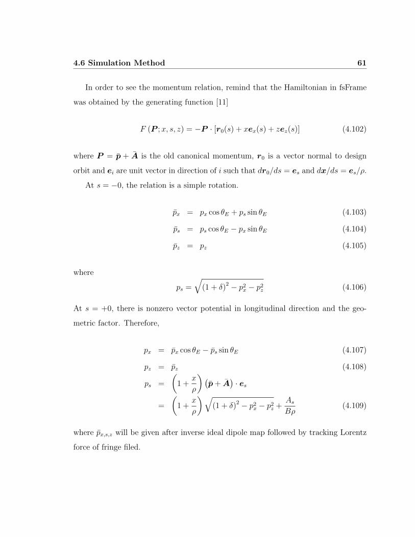
4.6 Simulation Method 61
In order to see the momentum relation, remind that the Hamiltonian in fsFrame
was obtained by the generating function [11]
F (P ;x, s, z) = −P · [r0(s) + xex(s) + zez(s)] (4.102)
where P = p + A is the old canonical momentum, r0 is a vector normal to design
orbit and ei are unit vector in direction of i such that dr0/ds = es and dx/ds = es/ρ.
At s = −0, the relation is a simple rotation.
px = px cos θE + ps sin θE (4.103)
ps = ps cos θE − px sin θE (4.104)
pz = pz (4.105)
where
ps =
√(1 + δ)2 − p2
x − p2z (4.106)
At s = +0, there is nonzero vector potential in longitudinal direction and the geo-
metric factor. Therefore,
px = px cos θE − ps sin θE (4.107)
pz = pz (4.108)
ps =
(1 +
x
ρ
)(p+ A
)· es
=
(1 +
x
ρ
)√(1 + δ)2 − p2
x − p2z +
AsBρ
(4.109)
where px,s,z will be given after inverse ideal dipole map followed by tracking Lorentz
force of fringe filed.

4.6 Simulation Method 62
4.6.5 Simulation Steps for Thin Map
A effective thin map can be obtained by sandwiching the back transforms of drift
and dipole at the each end of the fringe field map. As for dipole entrance, we used
following steps.
• Transform from fsFrame to rFrame
• Back drift to s = −L
• Apply the leap-frog method until the particle reach at s = L
• Back transform using ideal dipole field until the particle reach at s = −x tan θE
which corresponds to s = 0.
• Transform back to fsFrame
4.6.6 Magnetic Field Setting for Simulation
Throughout the simulation we use the logistic functional fringe field,
φ01(s) =1/ρ
1 + exp (−s/g)
φ21(s) = 0
See Eq. (4.7). This setting gives simple analytic expression for field integration pa-
rameters.
K0 = π2/6 K2 = 1 K3 = 1/6 K1,4,5,6 = 0

4.7 Simulation Result 63
4.7 Simulation Result
4.7.1 Cloed Orbit Deviation
The closed orbit effect can be checked by setting all the initial canonical variables
to zero, i.e., x = z = px = pz = δ = 0. In this simulation θE = π/8 is used as an
example. The simulation results for dipole entrance with various values of g and ρ
are shown in Fig. 4.6 and Fig. 4.7. They show good agreement with our derivation.
Remind from Eq. (4.74) and Eq. (4.76) that the closed orbit deviation at dipole
entrance is order of
∆xco ∝ −g2K0/ρ
∆px,co ∝ −g2K0/ρ2
In the same way, the fringe field closed orbit effect at dipole exit is shown in
Fig. 4.8 and Fig. 4.9. From Eq. (4.78) and Eq. (4.80), the closed orbit deviation at
dipole exit is order of
∆x ∝ g2K0/ρ
∆px ∝ O(g3/ρ2
)→ Fitted to ∆px = 0.212 g3/ρ2
where the simulated closed orbit momentum deviation is numerically fitted to g3/ρ2
which is corresponds to an approximation error.

4.7 Simulation Result 64
2 4 6 8 10
−12
−10
−8
−6
−4
−2
ε [cm]
∆ x
[mm
]
ρ=1
ρ=3
ρ=5
ρ=10
∆ x∆ x
theory
Figure 4.6: ∆xco at dipole entrance. The red marks are simulationdata and blue line is the theoretical prediction.
2 4 6 8 10
−3
−2.5
−2
−1.5
−1
−0.5
0
x 10−3
ε [cm]
∆ p x
ρ=1ρ=3
ρ=5ρ=10
∆ px
∆ px,theory
Figure 4.7: ∆px,co at dipole entrance
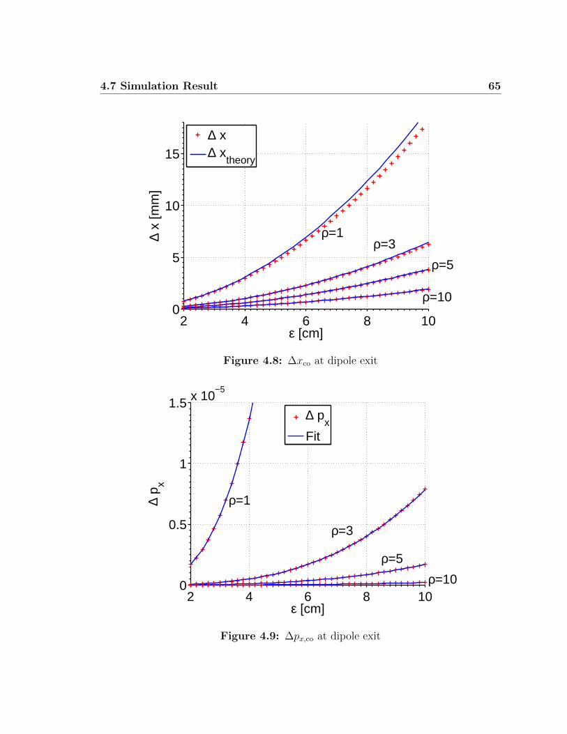
4.7 Simulation Result 65
2 4 6 8 100
5
10
15
ε [cm]
∆ x
[mm
]
ρ=1ρ=3
ρ=5
ρ=10
∆ x∆ x
theory
Figure 4.8: ∆xco at dipole exit
2 4 6 8 100
0.5
1
1.5 x 10⁻⁵
ε [cm]
∆ p x
ρ=1
ρ=3
ρ=5
ρ=10
∆ px
Fit
Figure 4.9: ∆px,co at dipole exit

4.7 Simulation Result 66
4.7.2 Octupole Like Potential Effect
Since, we have good agreement with [13] up to the sextupole-like potential, we
jump to verify octupole-like potential effect which present in the following differential.
See Eq. (4.77)∂3
∂z3∆pz =
K3
(1 + δ)ρ2g
[4
cos θE− 8
cos3 θE
](4.110)
Note that the octupole-like potential is inverse proportional to fringe field extent. In
order to verify the differential, we exploit the automatic differentiation technique [26].
The theoretical and simulated values of the differential ∂3z∆pz shows good agreement
in Fig. 4.10.
2 4 6 8 1010
−1
100
101
ε [cm]
−∂3 z (
∆ p z)
[m−
3 ]
ρ=1
ρ=3
ρ=5
ρ=10
simulationtheory
Figure 4.10: Octupole-like potential effect on ∂3z∆pz

4.8 Example : TTX 67
4.8 Example : TTX
In this section, we test detuning parameters and chromaticities on Tsinghua
Thomson scattering x-ray(TTX) source ring which is 4.8 meter long and as illus-
trated in Fig. 3.1, it consists of pair of quadrupoles which are used to adjust damping
partition number and four dipoles whose edge angles are chosen for a proper tune [6].
When the focusing correction of dipole fringe field effect is considered with g = 0.9
and K1 = 0.9, the edge angles and focusing quadrupole strength are chosen by
EdgeAngles = 0.64577182323 rad
QuadStrength = 30 m−2
Then, each order of nonlinearities of the dipole fringe field mapping equations are
turned on step by step while particles are tracked to measure chromaticities and
nonlinear detuning parameters. The result is written down in Table 4.1
Table 4.1: The effect of nonlinear fringe field on chromaticities andnonlinear detuning parameters of TTX. αij are the non-linear detuning parameters of dimension [m−1], and ξiare the chromaticity.
Switch αxx αxz αzz ξx ξz
Kinetic 20.3 5.84 12.4 -2.09 -0.993rd Order H 14.6 669 389 -1.81 -9.714rd Order H 14.5 669 1021 -1.81 -9.71
Next, we turned on K0 which is responsible for the closed orbit deviation, and
searched for the fixed point. Fig. 4.11 shows the result. Note that the closed orbit
of several mm is generated. As the beam pipe radius is several mm, there can be
severe beam loss. The concave corresponds to dipole location and the convex corre-
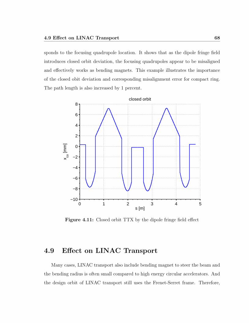
4.9 Effect on LINAC Transport 68
sponds to the focusing quadrupole location. It shows that as the dipole fringe field
introduces closed orbit deviation, the focusing quadrupoles appear to be misaligned
and effectively works as bending magnets. This example illustrates the importance
of the closed obit deviation and corresponding misalignment error for compact ring.
The path length is also increased by 1 percent.
0 1 2 3 4 5−10
−8
−6
−4
−2
0
2
4
6
8closed orbit
s [m]
x co [m
m]
Figure 4.11: Closed orbit TTX by the dipole fringe field effect
4.9 Effect on LINAC Transport
Many cases, LINAC transport also include bending magnet to steer the beam and
the bending radius is often small compared to high energy circular accelerators. And
the design orbit of LINAC transport still uses the Frenet-Serret frame. Therefore,
4.10 Nonlinear Detuning by octupole like potential 69
same rule applies. The closed orbit deviation can be especially important for the
injection matching.
4.10 Nonlinear Detuning by octupole like poten-
tial
One of the interesting effects of the octupole like potential is the detuning ef-
fect. Since a Lie map generator of an accelerator element is an effective Hamiltonian
multiplied by length of the element, we find the effective octupole like potential of
Eqs. (4.62, 4.73) can be written as
Hoct = δ(s)z4
4!
[4
cos θE− 8
cos3 θE
]K3
ρ2g(4.111)
where δ(s) indicate the Dirac delta function at a dipole edge location of either entrance
and exit. Therefore, the vertical nonlinear detuning parameter is
αzz = − 1
16π
[4
cos θE− 8
cos3 θE
]K3
ρ2g
∫dsβ2
z (s)δ(s) ds
' −β2z (0)
16π
[4
cos θE− 8
cos3 θE
]K3
ρ2g(4.112)
where, in the last line, we assumed that the betatron function does not change much
across the edge, i.e., βz(0−) ' βz(0+) which usually is true. Note that it is inversely
proportional to fringe field extent. By dimensional analysis, the sextupole like po-
tential of the fringe field edge will contribute to the nonlinear detuning parameter
by order of O(β2xβz/ρ
4). Therefore, the effect by octupole like potential on nonlinear
detuning parameter can be larger as the fringe field extent become shorter.

4.11 Conclusion 70
4.11 Conclusion
We derived the effective thin Lie map generator and mapping equations of trans-
verse dynamics for dipole fringe field up to octupole-like potential. Two major findings
were the closed orbit deviation which is order of g2/ρ, and the octupole-like potential
which is order of 1/(gρ2). These two effects were not included in SLAC-75 [13].
The closed orbit effects depend mainly on two field integration parameters K0
and K1. The field integration parameter K1 must vanish by definition or equivalently
by dipole design in order to have intended bending angle as the design orbit. We
also showed that the closed deviation can be large enough to graze the beam pipe for
compact ring.
The octupole-like potential was shown to be inversely proportional to fringe field
extent. Similarly, higher order nonlinearities are expected to be inversely proportional
to the higher power of fringe field extent.
Therefore, a careful dipole fringe field design will be needed for the compromise
between the closed orbit and nonlinearities. For example, when the beam emittance
is small, the closed orbit deviation is more important concern than the nonlinearities.
Therefore, one would like to minimize the fringe field extent in this case.
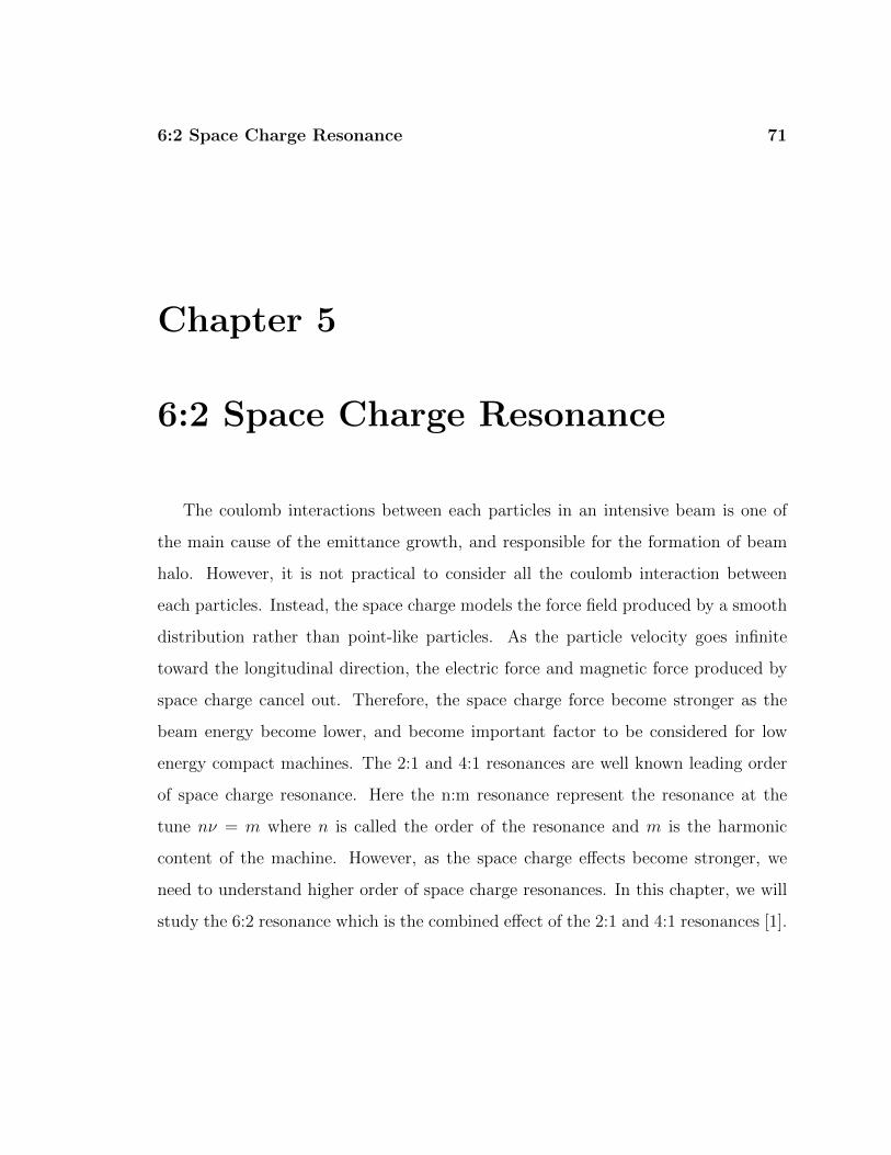
6:2 Space Charge Resonance 71
Chapter 5
6:2 Space Charge Resonance
The coulomb interactions between each particles in an intensive beam is one of
the main cause of the emittance growth, and responsible for the formation of beam
halo. However, it is not practical to consider all the coulomb interaction between
each particles. Instead, the space charge models the force field produced by a smooth
distribution rather than point-like particles. As the particle velocity goes infinite
toward the longitudinal direction, the electric force and magnetic force produced by
space charge cancel out. Therefore, the space charge force become stronger as the
beam energy become lower, and become important factor to be considered for low
energy compact machines. The 2:1 and 4:1 resonances are well known leading order
of space charge resonance. Here the n:m resonance represent the resonance at the
tune nν = m where n is called the order of the resonance and m is the harmonic
content of the machine. However, as the space charge effects become stronger, we
need to understand higher order of space charge resonances. In this chapter, we will
study the 6:2 resonance which is the combined effect of the 2:1 and 4:1 resonances [1].
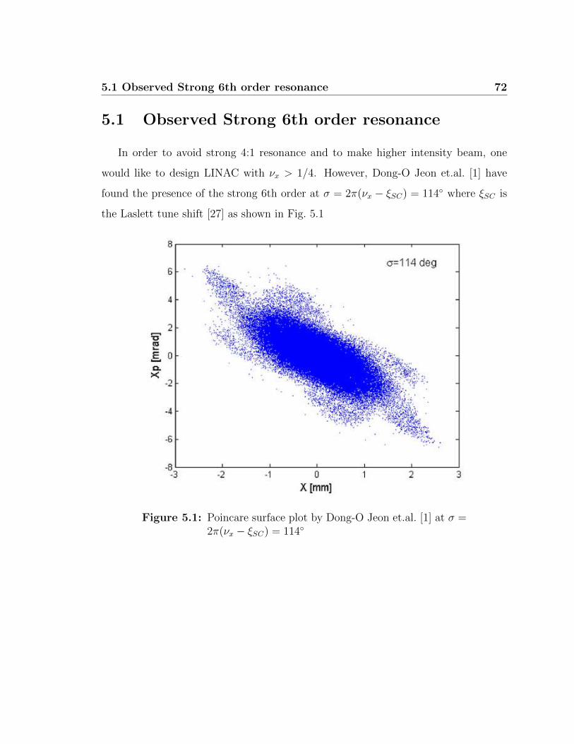
5.1 Observed Strong 6th order resonance 72
5.1 Observed Strong 6th order resonance
In order to avoid strong 4:1 resonance and to make higher intensity beam, one
would like to design LINAC with νx > 1/4. However, Dong-O Jeon et.al. [1] have
found the presence of the strong 6th order at σ = 2π(νx − ξSC) = 114 where ξSC is
the Laslett tune shift [27] as shown in Fig. 5.1
Figure 5.1: Poincare surface plot by Dong-O Jeon et.al. [1] at σ =2π(νx − ξSC) = 114

5.2 Explanation 73
5.2 Explanation
In order to understand the 6:2 resonance, we explore the space charge Hamiltonian
for 2D Gaussian beam
H(x,p; s) =p2x + p2
z
2+Kx
2x2 +
Kz
2z2 + VSC
VSC(x,p; s) = −KSC
2
[x2
a (a+ b)+
z2
b (a+ b)
]+
KSC
8a2 (a+ b)2
[2 + r
3x4 +
2
rx2z2 +
1 + 2r
3r3z4
]− KSC
144a3 (a+ b)3
[8 + 9r + 3r2
5x6 +
3 (3 + r)
rx4z2 + . . .
]+ . . . (5.1)
where s is the longitudinal coordinate on reference orbit which is the independent time
variable for this Hamiltonian system, Kx(s) and Kz(s) are focusing field strength,
a2 = βxεx, b2 = βzεz are beam size and r = b/a. Since we are interested in 6:2
resonance in horizontal plane, the 1D Hamiltonian can be approximated as
H(x, px; s) =p2x
2+Kx
x2
2− V2x
2 + V4x4 − V6x
6 + · · · (5.2)
where the signs are chosen such that the each space charge potential coefficients Vi
are positive.
The focusing function Kx(s) = Kx(s + L) is a periodic over the period L. The
periodicity on space charge potential V2(s) = V2(s + L) and V4(s) = V4(s + L) also
hold approximately because the matched beam core breathe following the lattice
functions. Therefore, we can use the Floquet transformation x =√
2βxJx cos Φx,
where Φx = φx + χx − νxθ with χx =∫ s
01βxds, θ = 2πs/L is the orbiting angle, and
Jx and φx are canonical conjugate variables of action-angle. Then, we obtain the

5.2 Explanation 74
following Hamiltonian:
H(φx, Jx; θ) = νxJx−L
2πV2βxJx−
L
2πV2βxJx cos 2Φx+
L
2πV4β
2xJ
2x
3 + 4 cos 2Φx + cos 4Φx
2.
(5.3)
where L is the length of the periodic cell and the orbital angle θ plays the role of
independent time variable. Note that we have 2:1 and 4:1 resonance terms which are
proportional to Jx and J2x respectively. On the other hand, the 6:1 resonance term
which can be explicitly seen from the space charge potential in Eq. (5.2) is propor-
tional to J3x , hense, it is a weak resonance. In addition, recall that the simulation
setting on the single cell tune was close to 1/3. Therefore, what we can think of the
origin of the 6:2 is the combination effect of 2:1 and 4:1 resonances.
Keeping both 2:1 and 4:1 resonance terms, we approximate the Hamiltonian as
follows:
H = νxJx − ξxJx + αxxJ2x
2+G2Jx cos (2φx − θ + η2) +G4J
2x cos (4φx − θ + η4) + . . .
(5.4)
where
ξx =1
2π
∫ L
0
V2βx ds (5.5)
αxx =3
2π
∫ L
0
V4β2x ds (5.6)
G2eiη2 = − 1
2π
∫ L
0
V2βxei[2χx−(2νx−1)θ] ds (5.7)
G4eiη4 =
1
4π
∫ L
0
V4β2xei[4χx−(4νx−1)θ] ds. (5.8)
Remember that ξx and αxx are positive.
In order to combine the strong 2:1 and 4:1 resonance terms we use parameterized
canonical perturbation to cancel out the 2:1 and 4:1 resonance terms and bring the

5.2 Explanation 75
6:2 resonance term appear. For this purpose, we introduce the following generating
function
F2(φx, Ix) = φxIx +B2(Ix) sin(2φx − θ + η2) +B4(Ix) sin(4φx − θ + η4) (5.9)
where (φx, Jx) and (ψx, Ix) are old and new conjugate phase space coordinates, and
B2 and B4 terms are chosen to cancel out the the 2:1 and 4:1 resonances respectively.
Then, we find the new Hamiltonian is
H ' νxIx − ξxIx + αxxI2x
2+ (νx − ξx + αxxIx)∆J +
αxx2
∆J2
+(IxG2 −B2)C2 + (I2xG4 −B4)C4 + (2IxC4G4 − C2G2)∆J (5.10)
where,
∆Jx = Jx − Ix = 2B2C2 + 4B4C4
Sn = sin (nφx − θ + ηn)
Cn = cos (nφx − θ + ηn) .
It can be re-written in terms of the canonical variables by
H = νxIx − ξxIx + αxxI2x
2
+(2B2G2 + 2B2αxx)C22 + (8B4G4Ix + 8B2
4αxx)C24
+(G2Ix + δ2B2 + 2B2αxxIx)C2 + (G4I2x + δ4B4 + 4B4αxxIx)C4
+(4B4G2 + 4B2G4Ix + 8B2B4αxx)C2C4 (5.11)
where C2 and C4 corresponds to 2:1 and 4:1 resonance driving terms, and C2C4 is the

5.2 Explanation 76
term what we want to make the 6:2 resonance term to appear explicitly, and
δn ≡ n (νx − ξx)− 1 (5.12)
In order to cancel out the 2:1 and 4:1 resonance terms in the Hamiltonian, we set
B2 = − G2Ixδ2 + 2αxxIx
B4 = − G4I2x
δ4 + 4αxxIx
Next, we average over the fast oscillation near the 6:2 resonance tune, so that 〈C2n〉 =
〈S2n〉 = 1/2, and other oscillation terms except 6:2 resonance term are washed out.
Then,
H ≈(νx − ξx −
G22
δ2
)Ix+αxx
(1 + 6
G22
δ22
)I2x
2+G6:2I
2x cos (6ψ − 2θ + η2 + η4) (5.13)
where
G6:2 ≡ −2G2G4
δ2δ4
(6νx − 6ξx − 2) (5.14)
Eq. (5.13) can be made further simpler by canonical transformation into resonance
rotating frame. For this purpose we use the following generating function
F2 = (ψx −1
3θ +
1
6η2 +
1
6η4)I (5.15)
whose conjugate variables are I = Ix, and φ = (ψx − 13θ+ 1
6η2 + 1
6η4). Then, the new
Hamiltonian is
H =
(νx −
1
3ξx −
G22
δ2
)I + αxx
(1 + 6
G22
δ22
)I2
2+G6:2I
2 cos(6φ) (5.16)

5.3 Simulation 77
We finally made the 6:2 resonance driving term to be explicitly shown. One of the
most important finding is that the resonance driving strength is proportional to I2x
instead of I3x. Therefore it is a strong resonance. Another important finding is that
the 6:2 resonance must occur when νx >13. Less importantly, since αxx is the positive,
as the tune ramp down, the resonance islands will move away from the origin.
5.3 Simulation
In order to verify the theoretical explanation, few simulations are carried out using
frozen distribution method [28]. 4000 macro-particles are tracked on simple FODO
cells. The bare tune for each cell is set to 0.334 which is slight larger than 1/3 so that
the Laslett tune push the reduced tune less than 1/3. Since the detuning parameter
is positive, the 6th order resonance islands appear further and further away as the
space charge perveance increases. It is well described in Fig. 5.2.
5.4 conclusion
We found that the 6:2 resonance can be understood by combined effect of 4:1
and 2:1 resonances. And unlike 6:1 resonance, it appears near ν = 1/3 and is a
strong resonance because G6:2 ∝ I2 . In addition, the resonance occurs only when
νx + ξx < 1/3 and νx > 1/3.

5.4 conclusion 78
Figure 5.2: Phase space plot on FODO cells. The bare tune is setto νx = 0.339. From left to right and top to bottom,the particle line density is increasing and the reducedtune per cell are found to be 0.334, 0.324, 0.314, 0.304,0.295 and 0.285

Explicit Symplectic Tracking for Electric Ring 79
Chapter 6
Explicit Symplectic Tracking for
Electric Ring
The high energy charged particles have smaller rigidity in magnetic fields com-
pared to the electric fields. For this reason, most of high energy accelerator lattices are
composed of magnetic elements. However, interest on and applications of electrostatic
storage rings and synchrotrons on low energy ions are increasing recently. For exam-
ple, Refs. [29][30] demonstrates the success of the electrostatic storage rings for the
low-medium energy atomic physics research. More recently, the electrostatic storage
rings are proposed for electric dipole moment (EDM) search. They are also consid-
ered and designed for biomolecular study [31]. Therefore, it is important to build
and benchmark precise and explicit symplectic numerical particle tracking codes for
electrostatic fields. However, most of the present tracking codes are for magnetic field
elements. And as we will see later, the construction of explicit symplectic tracking
code for electric element is a difficult task. There are few codes that able to do this
job : ETEAPOT [33] and COSYinfinity [34]. However, ETEAPOT assumes inverse square
force law where the exact solution of the particle orbit and spin trajectory is available.

6.1 Problem 80
The general force fields are modeled with additional virtual quadrupole correctors.
On the other hand, COSYinfinity [34] is differential algebra (DA) based. And the
DA map requires truncation of the power series and artificial symplectification. It
is true that the high order truncation can be made to closely reproduce the exact
solution. However, when there is significant change of lattice design, the DA map
need to be re-calculated. Therefore it is less flexible.
6.1 Problem
The difficulty of building an explicit symplectic integrator for electric elements
can be seen easily from the Eq. (2.7) which is re-written here,
H (x, Px, z, Pz, t,−E; s)
= −(
1 +x
ρ
)√(E − qΦ)2
c2−m2c2 − P 2
x − P 2z (6.1)
where E is the particle energy, q is the charge, m is the mass, c is the speed of light,
Φ is the electric potential, ρ is the curvature, t is the time of flight in the lab frame
and (x, Px, z, Pz) are horizontal and vertical conjugate variables respectively. Note
also that the electric potential Φ is coupled with the particle energy E under the
square-root, thus highly nonlinear. In addition, since the Hamiltonian Eq. (6.1) is
composed of single term, the splitting method which will be illustrated in Sec 6.2 is
not applicable.
6.2 Splitting and Composition method revisited
Here we give brief review on splitting and compostion method of numerical track-
ing [38].

6.2 Splitting and Composition method revisited 81
6.2.1 Splitting Method
Consider an autonomous differential equation dy/dt = L(y). If it can be split
into m exactly solvable parts y = Li(y), where L = L1 +L2 + · · ·+Lm, whose exact
flows are fi (t), the following map is the 1st order method
M1 (t) = f1 (t) f2 (t) · · · fm (t) (6.2)
6.2.2 Self Adjoint Map
Consider the exact flow f(t) : y(0)→ y(t) of an autonomous differential equation
dy/dt = L(y). Then the reverse flow can be obtained by time reversal t → −t such
that f(−t)−1 = f(t). However, this is generally not true for a numerical map F (t)
like the Euler method [38]. In this regards, F−1(−t) is called adjoint of F (t) and the
self-adjoint map F−1(−t) = F (t) is called symmetric. Then, one can easily see that
the self-adjoint map F (t) is odd function of t and thus is an even order method.
6.2.3 Composition Method
The composition method is the procedure of building higher order maps out of
the lower ones. Consider the following composition map
M(t) = F (κmt) · · · F (κ2t) F (κ1t) (6.3)
where F (t) is an one step method of order r and step size t and κit are the step sizes
and is the composition operator. Then, it can be shown that if
κ1 + · · ·+ κm = 1 (6.4)
κr+11 + · · ·+ κr+1
m = 0,

6.2 Splitting and Composition method revisited 82
the composition methodM(t) is at least r+1 order map [38]. In addition, if F (t) is a
symmetric map and the step sizes are chosen to be symmetric such that κi = κm−i+1,
then M(t) is also symmetric and thus it become at least r + 2 order map. And of
course if the basic map F (t) is symplectic Hamiltonian flow, the composition map
M(t) is also symplectic. For example, the Yoshida’s formalism [37], which is well
known in accelerator community, belongs to such a symmetric composition method
with
κ1 = κ3 =1
2− 21/2r+1, κ2 = − 21/2r+1
2− 21/2r+1(6.5)
In general, there are infinite number of possible choices of κi. Such procedures can be
numerically optimized to reduce both the number of steps and numerical error. For
example, the optimized 6th order symmetric map M(t) out of 2nd order symmetric
map is given by [38].
κ1 = κ7 = 0.78451361047755726382
κ2 = κ6 = 0.23557321335935813368
κ3 = κ5 = −1.17767998417887100695 (6.6)
κ4 = 1.31518632068391122204

6.3 Hamiltonian 83
Same way, the optimized 8th order symmetric mapM(t) out of 2nd order symmetric
map is given by [38].
κ1 = κ15 = 0.74167036435061295345
κ2 = κ14 = −0.40910082580003159400
κ3 = κ13 = 0.19075471029623837995
κ4 = κ12 = −0.57386247111608226666
κ5 = κ11 = 0.29906418130365592384 (6.7)
κ6 = κ10 = 0.33462491824529818378
κ7 = κ9 = 0.31529309239676659663
κ8 = −0.79688793935291635402
The performance of different methods are illustrated in [38] which shows that higher
order optimized methods is more precise than low order ones for long term tracking.
6.3 Hamiltonian
6.3.1 Lorentz Covariant Hamiltonian
Ref. [39] introduced the following Lorentz covariant Hamiltonian for explicit sym-
plectic tracking over the s-dependent magnetic field region.
H (xµ, P µ; τ) =1
2m(P µ − qAµ) (Pµ − qAµ) (6.8)
where the metric tensor is assumed to be gµν = diag(1,−1,−1,−1), and P µ and Aµ
are contravariant 4-momentum and 4-potential respectively. Note that the Hamilto-
nian value is a constant H = mc2/2. Note also that the Hamiltonian is autonomous

6.3 Hamiltonian 84
even in the presence of RF components. The equivalent Hamiltonian [39] for the
conventional time and space is K = −H.
K (x,P , t,−E; τ) =(P − qA)2
2m− (E − qΦ)2
2mc2(6.9)
where P = mcβγ+qA is the classical canonical momentum and E = cP 0 = mc2γ+qΦ
is the total particle energy which also is a canonical momentum in this Hamiltonian
system. It is important to remember that the independent time variable of this
Hamiltonian is the proper time τ .
6.3.2 Normalization and Canonical Transformation
Let K be the old Hamiltonian and T the normalized new Hamiltonian such that
T = sxpK where x, p, and s are the normalization factors. Then the canonical variables
of each system are related by
dp
ds= −∂K
∂x= −
(xp
s
)∂T
∂x→ d (p/p)
d (s/s)=
∂T
∂ (x/x)(6.10)
dx
ds=
∂K
∂p=
(xp
s
)∂T
∂p→ d (x/x)
d (s/s)=
∂T
∂ (p/p)(6.11)
On the other hand, rigidity relations for electric and magnetic bending are
ρ0E0 = −mc2β2
0γ0
q(6.12)
ρ0B0 = −mcβ0γ0
q(6.13)
Therefore, we choose
• p = p0 = mcβ0γ0 for (x, px, z, pz)
• p = E0β20 = mc2γ0β
20 , and x = 1/β0c for (t,−E)
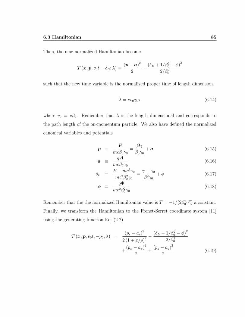
6.3 Hamiltonian 85
Then, the new normalized Hamiltonian become
T (x,p, v0t,−δE;λ) =(p− a)2
2− (δE + 1/β2
0 − φ)2
2/β20
such that the new time variable is the normalized proper time of length dimension.
λ = cv0γ0τ (6.14)
where v0 ≡ cβ0. Remember that λ is the length dimensional and corresponds to
the path length of the on-momentum particle. We also have defined the normalized
canonical variables and potentials
p ≡ P
mcβ0γ0
=βγ
β0γ0
+ a (6.15)
a ≡ qA
mcβ0γ0
(6.16)
δE ≡ E −mc2γ0
mc2β20γ0
=γ − γ0
β20γ0
+ φ (6.17)
φ ≡ qΦ
mc2β20γ0
(6.18)
Remember that the the normalized Hamiltonian value is T = −1/(2β20γ
20) a constant.
Finally, we transform the Hamiltonian to the Frenet-Serret coordinate system [11]
using the generating function Eq. (2.2)
T (x,p, v0t,−p0;λ) =(ps − as)2
2 (1 + x/ρ)2 −(δE + 1/β2
0 − φ)2
2/β20
+(px − ax)2
2+
(pz − az)2
2(6.19)

6.3 Hamiltonian 86
6.3.3 Splitting
For later convenience of applying the splitting method, we nominate each term of
the Hamiltonian by
Tx ≡(px − ax)2
2, Tz ≡
(pz − az)2
2
Ts ≡(ps − as)2
2 (1 + x/ρ)2 , TE ≡ −(δE + 1/β2
0 − φ)2
2/β20
such that T = Tx + Tz + Ts + TE. For example, when each of splitted Hamiltonian
are solvable, the 1st order integrator can be built by
M1(λ) = e−λ :Tx:e−λ :Tz:e−λ :Ts:e−λ :TE :. (6.20)
And we built the 2nd order map, by concatenation with an adjoint map,
M2(λ) =M−11
(−λ
2
)M1
(λ
2
)(6.21)
such that M2 is a symmetric method. From now on, we will call Eq. (6.19) as
τ -domain Hamiltonian and Eq. (6.22) as s-domain Hamiltonian.
6.3.4 s-domain Hamiltonian
The conventional s-domain Hamiltonian can be obtained by the chain rule. For
example, using
dT =
(∂T
∂px
)dpx +
(∂T
∂ps
)dps = 0
dT =
(∂T
∂x
)dx+
(∂T
∂ps
)dps = 0,
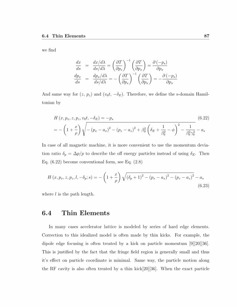
6.4 Thin Elements 87
we find
dx
ds=
dx/dλ
ds/dλ=
(∂T
∂ps
)−1(∂T
∂px
)=∂ (−ps)∂px
dpxds
=dpx/dλ
ds/dλ= −
(∂T
∂ps
)−1(∂T
∂px
)= −∂ (−ps)
∂px
And same way for (z, pz) and (v0t, −δE). Therefore, we define the s-domain Hamil-
tonian by
H (x, px, z, pz, v0t,−δE) = −ps (6.22)
= −(
1 +x
ρ
)√− (px − ax)2 − (pz − az)2 + β2
0
(δE +
1
β20
− φ)2
− 1
β20γ
20
− as
In case of all magnetic machine, it is more convenient to use the momentum devia-
tion ratio δp = ∆p/p to describe the off energy particles instead of using δE. Then
Eq. (6.22) become conventional form, see Eq. (2.8)
H (x, px, z, pz, l,−δp; s) = −(
1 +x
ρ
)√(δp + 1)2 − (px − ax)2 − (pz − az)2 − as
(6.23)
where l is the path length.
6.4 Thin Elements
In many cases accelerator lattice is modeled by series of hard edge elements.
Correction to this idealized model is often made by thin kicks. For example, the
dipole edge focusing is often treated by a kick on particle momentum [9][20][36].
This is justified by the fact that the fringe field region is generally small and thus
it’s effect on particle coordinate is minimal. Same way, the particle motion along
the RF cavity is also often treated by a thin kick[20][36]. When the exact particle

6.5 Explicit Symplectic Tracking in Transverse Magnetic Elements 88
motion in those field region is important, such a thin kick treatment can be replaced
by more precise tracking methods any time. Therefore, we adopt the simple kick
modeling for fringe field and RF-cavity. Especially, since the longitudinal momentum
ps is the canonical variable in the τ -domain Hamiltonian, we employ a kick model on
ps at every entrance of lattice elements by Eq. (6.22). It is worth to mention that
such a treatment is automatically included in s-domain Hamiltonian which is not
autonomous and whose value is −ps. In case of RF-cavity, we use the following kick
model [11]
∆δE =VRF
mc2γ0β20
sin (2πωRF t+ φs) (6.24)
where VRF is the effective RF voltage, ωRF is the RF angular frequency and φs is the
RF phase. Of course the kick on ps is required additionally to Eq. (6.24) for τ -domain
tracking.
6.5 Explicit Symplectic Tracking in Transverse Mag-
netic Elements
In general, s-domain tracking is much easier and faster than the τ -domain tracking
for magnetic field. However, as we will see later, the s-domain tracking can introduce
numerical error on closed orbit at bending magnet and such an effect can be important
for compact machine. In addition, we want to compare the τ -domain tracking with
conventional s-domain tracking. Therefore, we present τ -domain tracking method for
transverse magnetic elements and compare with a conventional tracking code MADX
PTC module [23].
Throughout this section, we assume transverse magnetic field such that ax = az =
φ = 0 and as = as(x, z). Then the Hamiltonian can be separable into exactly solvable
parts: The drift part TxzE ≡ Tx + Tz + TE and the field strength kick part Ts. Then,

6.5 Explicit Symplectic Tracking in Transverse Magnetic Elements 89
the second order symmetric and symplectic integrator can be built by
M2(λ) = e−λ
2:TxzE :e−λ :Ts:e−
λ
2:TxzE : (6.25)
Among them, the drift part is straight forward. Since,
TxzE =p2x + p2
z
2− (δE + 1/β2
0)2
2/β20
(6.26)
the action of e−λ :TxzE : is simply
∆x = pxλ, ∆z = pzλ, v0∆t =(1 + δEβ
20
)λ (6.27)
While, the magnetic field kick part is
Ts =(ps − as)2
2 (1 + x/ρ)2 (6.28)
Therefore, the action of e−λ :Ts: is
∆s = λ(ps − as)
(1 + x/ρ)2 (6.29)
∆px = λ(ps − as) [(ps − as) /ρ+ (1 + x/ρ) ∂xas]
(1 + x/ρ)3 (6.30)
∆pz = λ (ps − as) ∂zas (6.31)
6.5.1 Reaching exact end of an element
The τ -domain Hamiltonian promoted the longitudinal coordinate s to one of the
canonical variables which makes the code hard to track a particle for an exact length
L of an element. We solve this problem by, first, adjusting the step size of the last
integration and second, adding one more integration step to the supposed-to-be-last

6.5 Explicit Symplectic Tracking in Transverse Magnetic Elements 90
integration step in order to make correction to the remaining or extra length the
particle need to be tracked. Specifically, it can be shown that
M2(λ)s = s+ps − as
(x→ x+ px
λ2, z → z + pz
λ2
)[1 +
(x+ px
λ2
)/ρ]2 λ (6.32)
Then, the required step size of an integrator to track ∆s can be calculated. For
example, in case of the magnetic sector bend the required step size to track the
length ∆s is, by Eq. (6.32),
λ =(1 + x/ρ)2
ps − as∆s+
(2ps − 1) (1 + x/ρ)3
2 (ps − as)3 px∆s2
ρ+O
(∆s3
)(6.33)
The 3rd order of ∆s is irrelevant because the integration method is already 2nd
order, and the remaining or extra length ∆s is generally small. Same way, in case of
magnetic quadrupole, we find
λ =∆s
ps − as− k1
pxx− pzz2 (ps − as)3 ∆s2 +O
(∆s3
)(6.34)
As we will show in the next section, this treatment is proved to reduce the remaining
or extra length ∆s to the machine error compared to the length L of an element in a
possible worst scenario.
6.5.2 Numerical Error on Closed Orbit
Note that for magnetic bending, Eq. (6.23) can be separable into the drift part
D ≡ H+as and the field strength kick part −as. And there is cancelation between the
closed orbit kick by the drift part which is introduced by the geometric factor 1+x/ρ
and the closed orbit kick by bending magnet strength. However, the numerical can-
cellation is not perfect and such an imperfection can be be sizable for a very compact

6.5 Explicit Symplectic Tracking in Transverse Magnetic Elements 91
machine like Tsinghua Thomson scattering X-ray source (TTX) [6] whose bending
radius is ρ = 0.25m. This fact is illustrated well in Fig 6.1. A particle is prepared
initially on reference orbit of TTX and tracked using MADX PTC module [23] with the
4-th order symplectic method. Since, the τ -domain kick Hamiltonian includes both
of the geometric and bending magnet field kick in a single step e−∆λ:Ts:, no numerical
closed orbit error is introduced which also is well illustrated in Fig. 6.1.
-10
-5
0
5
10
-10 -8 -6 -4 -2 0
p x [µ
rad]
x [µm]
Mad 10KicksMad 20KicksTim 10Kicks
-1
-0.5
0
0.5
1
-0.7 -0.3 0.1
Figure 6.1: Numerical Closed Orbit Error. MAD represent MADX
PTC module [23], and Tim represent the τ -domaintracking. The test lattice is TTX [6]. The number ofintegration step for all the magnetic elements is chosento be 10 and 20, and represented by 10Kicks and 20Kicks
repectively.

6.5 Explicit Symplectic Tracking in Transverse Magnetic Elements 92
6.5.3 Comparison with MADX PTC module
We also present a comparison between the τ -domain tracking code and a s-domain
tracking code MADX PTC module [23]. We used a simple 12 super period magnetic
FODO ring whose total length is 21.6m. Fig. 6.2 and Fig. 6.3 show good agreement
on transverse and longitudinal Poincare surface plots respectively.
-0.5-0.4-0.3-0.2-0.1
0
0.1 0.2 0.3 0.4 0.5
-0.8 -0.6 -0.4 -0.2 0 0.2 0.4 0.6 0.8
p x [m
rad]
x [mm]
TimTrackMadX
Figure 6.2: Poincare surface section of horizontal phase space.TimTrack represent the τ -domain tracking. The num-ber of integration step for all the magnetic elementsis chosen to be 100 for both of the tracking codes. 6particles of different initial x are tracked.
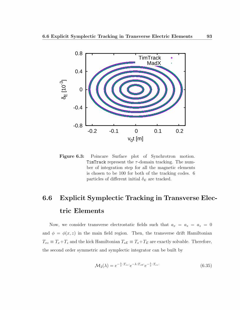
6.6 Explicit Symplectic Tracking in Transverse Electric Elements 93
-0.8
-0.4
0
0.4
0.8
-0.2 -0.1 0 0.1 0.2
δ E [1
0-3]
v0t [m]
TimTrackMadX
Figure 6.3: Poincare Surface plot of Synchrotron motion.TimTrack represent the τ -domain tracking. The num-ber of integration step for all the magnetic elementsis chosen to be 100 for both of the tracking codes. 6particles of different initial δE are tracked.
6.6 Explicit Symplectic Tracking in Transverse Elec-
tric Elements
Now, we consider transverse electrostatic fields such that ax = as = az = 0
and φ = φ(x, z) in the main field region. Then, the transverse drift Hamiltonian
Txz ≡ Tx+Tz and the kick Hamiltonian TsE ≡ Ts+TE are exactly solvable. Therefore,
the second order symmetric and symplectic integrator can be built by
M2(λ) = e−λ
2:Txz:e−λ :TsE :e−
λ
2:Txz: (6.35)

6.6 Explicit Symplectic Tracking in Transverse Electric Elements 94
6.6.1 Reaching exact end of an element
As we have already described in Sec. 6.5.1, finding the step size λ such that
M(λ)s = s + L is not a trivial task. Fortunately, it actually become trivial for
straight section elements of transverse electric field.
I Straight Section
In case of the transverse electric elements in straight section, one can be easily
show that
M (λ) s = s+ psλ (6.36)
Since, ps is conserved throughout the element under consideration, we can choose the
step size according to λ = L/Nps
where L is the length of the element and N is the
number of integration steps one can choose.
II Curved Section
However, in curved section, we follow the same strategy as described in Sec. 6.5.1.
Using the 2nd order integrator, one can find
M2 (λ) s = s+ps[
1 +(x+ px
λ2
)/ρ]2λ (6.37)
From which, the required step size of an integrator to track ∆s can be calculated by
λ =
(1 +
x
ρ
)2∆s
ps+ px
(1 +
x
ρ
)3∆s2
ρp2s
+O(∆s3
)(6.38)
Where O (∆s3) term is irrelevant because M2 is already the 2nd order map. Rest of
the procedure to reach the end of an element by tracking is described as Sec. 6.5.1.
One can tell that the error on ∆s become larger for smaller bending radius ρ by

6.6 Explicit Symplectic Tracking in Transverse Electric Elements 95
the dimensional analysis and by looking at Eq. (6.38). Therefore, we test our method
on an coaxial cylindrical electric dipole of very small bending radius ρ = 0.25m which
assumes a possible worst scenario. Table 6.1. shows the test result. Note that ∆s/L
is reduced to the double precision machine error where L is the length of an electric
dipole under consideration.
Table 6.1: Test of the method to reach the end of an element by τ -domain tracking. Standard deviation of ∆s is recordedwith one million particles whose initial value of phasespace set by Gaussian distribution with σ(x) = σ(z) =1mm, σ(px) = σ(pz) = 1mrad, and σ(δE) = 0.001where σ represent the standard deviation. The coaxialelectric bending of ρ = 0.25m and length= 0.4m isused. The 4th order integrator of Yoshida’s method isused. The number of integration is chosen to be 4 plusan additional step for correction. Action I is when theadjustment on the step size is made only for the lastintegration step among the 4 steps, and Action II iswhen additional correction integration step is made onremaining or extra ∆s after Action I
No Action Action I Action II
σ(∆s) [m] 2.08× 10⁻³ 8.40× 10⁻⁶ 4.71× 10⁻¹⁸
6.6.2 Comparision with the classical Runge-Kutta method
In order to prove our method in electric field, we compare the τ -domain track-
ing with the classical 4th order Runge-Kutta method. Although, the latter is not
symplectic, it can provide a good comparison reference for short-term tracking. The
lattice we used is 12 super period electric FODO ring whose total length is 21.6m.

6.6 Explicit Symplectic Tracking in Transverse Electric Elements 96
We used coaxial electric bending whose normalized potential is given by
φ = ln
(1 +
x
ρ
)(6.39)
and assumed the electric quadrupole potential by
φ = K1
(x2
2− z2
2
)(6.40)
where K1 is the normalized quadrupole field strength. The Poincare surface section
shown in Fig. 6.4. agrees well for both tracking methods.
-0.5
-0.4
-0.3
-0.2
-0.1
0
0.1
0.2
0.3
0.4
0.5
-0.8 -0.6 -0.4 -0.2 0 0.2 0.4 0.6 0.8
p x [m
mra
d]
x [mm]
TimTrack 10KicksRK4 100Kicks
Figure 6.4: Poincare surface plot of horizontal phase space.TimTrack represent the 4-th order symplectic τ -domain tracking and RK4 represent the classical Runge-Kutta method. The number of integration steps foreach dipoles are chosen to be 10 for TimTrack and 100for RK4. And the number of turns tracked are 100 mil-lion for TimTrack and 2048 turns for RK4

6.7 Conclusion 97
6.7 Conclusion
We have extended Ref. [39] to build an element-by-element orbit tracking code
based on Lorentz covariant Hamiltonian for electric elements. In order to compare
with the conventional tracking code, we also built the tracking code for magnetic
elements using the Lorentz covariant Hamiltonian. The agreement was successful.
During the course, we also found that this method can remove numerical error on
closed orbit which become important for very compact magnetic rings. There are no
symplectic tracking code for electric elements without approximation or power series
truncation so far. Therefore, it will be useful for the design of electric machine for
many applications including EDM measurement.

Conclusion 98
Chapter 6
Conclusion
The development of compact accelerators requires careful consideration of nonlin-
ear kinematics, magnet fringe field effects, high order space charge resonances, etc.
The nonlinear kinematics can add substantial nonlinearity to compact accelerators.
Indeed, it can limit the dynamic aperture even for a machine with all linear elements.
The contributions on nonlinear optics parameters are realized. And the analytic
expression can benefit the nonlinearity correction scheme.
The dipole fringe field introduces not only nonlinearity but also closed orbit devi-
ation. The high order nonlinear fringe effect is inverse proportional to the powers of
fringe field extent and the linear and low order nonlinear fringe field effect is propor-
tional to the powers of fringe field extent. Since, the range of fringe field is usually
minimized to avoid magnetic field coupling due to limited available space in compact
storage rings, there can be large high order nonlinear effect. In case of large beam
size, large vertical magnet gap is required. In this case, there can be large closed
orbit, linear focusing and low order nonlinear corrections. Therefore, design of com-
pact accelerators needs to have careful design of dipole fringe field to compromise low
order and high order effects. For example, the published TTX design concept may

Conclusion 99
fail because of large closed orbit excursion and large nonlinearities by dipole fringe
field.
In addition, the importance of high order of space charge resonance is realized.
The 6:2 space charge resonance originates the combination of 2:1 and 4:1 resonance.
And it is quite strong because it is proportional to the square of action pretty much
like 4:1 resonance. The 6:2 resonance occurs only when the bare tune is above 120.
Finally, an explicit symplectic tracking method for electric lattice elements is
presented. The electric accelerators are essentially compact because of small electric
rigidity compared to the magnetic rigidity. The particle motion along the design
orbit is highly nonlinear for electric elements which makes the explicit symplectic
method hard to be built. This difficulty could be solved by extending the canonical
varibles to include the longitudinal coordinate and momentum in Hamiltonian system
as described by Ref. [39].

BIBLIOGRAPHY 100
Bibliography
[1] Dong-O Jeon et.al., PRL 114, 184802 (2015)
[2] M. Venturini, R. Warnock, R. Ruth, and J. A. Ellison, Phys. Rev. ST Accel.
Beams 8, 014202 (2005).
[3] S. P. Moller and U. U. V. Pedersen, eds., Operational Experience with the Elec-
trostatic Storage Ring, ELISA, PAC (1999).
[4] E. Pozdeyev, CYCO and SIR: New Tools for Numerical and Experimental Stud-
ies of Space Charge Effects in the Isochronous Regime, Ph.D. thesis, Michigan
State University (2003).
[5] R. J. Loewen, A Compact Light Source: Design and Technical Feasibility Study
of a Laser-Electron Storage Ring X-Ray Source, Ph.D. thesis, Stanford University
(2003)
[6] H. S. Xu, W. H. Huang, C. X. Tang, and S. Y. Lee, Phys, Rev. ST Accel. Beams
17, 070101 (2014)
[7] D. Sagan and D. Rubin, Linear analysis of coupled lattices, Phys. Rev. ST Accel.
Beams 2, 074001 (1999)
[8] Hong Qin, Ronald C. Davidson, Joshua W. Burby, and Moses Chung, Analytical
methods for describing charged particle dynamics in general focusing lattices

BIBLIOGRAPHY 101
using generalized Courant-Snyder theory, Phys. Rev. ST Accel. Beams 17, 044001
(2014)
[9] Kilean Hwang and S. Y. Lee, Dipole fringe field thin map for compact syn-
chrotrons, Phys. Rev. ST Accel. Beams 18, 122401 (2015)
[10] Richard M. Talman, Measuring the Electric Dipole Moment of the Elec-
tron at Wilson Lab, The Cornell High Energy Synchrotron Source,
http://jclub.chess.cornell.edu/papers/TalmanWilsonElectronEDM-rev.pdf
(2013)
[11] S. Y. Lee, Accelerator Physics (third edition), World scientific (2011)
[12] M. Berz, B. Erdelyi, and K. Makino, Phys. Rev. ST Accel. Beams 3, 124001
(2000)
[13] K. L. Brown, SLAC Report-75 (1982)
[14] H. Matsuda and H. Wollnik, Nucl. Instrum. Methods 77 40 (1970)
[15] H. Matsuda and H. Wollnik, Nucl. Instrum. Methods 77 283 (1970)
[16] H. Matsuda and H. Wollnik, Nucl. Instrum. Methods 103 117 (1972)
[17] E. Forest, S.C. Leemann, and F. Schmidt, Fringe Effects in MAD PART I, Second
Order Fringe in MAD-X for the Module PTC, Tech. Rep.
[18] E. Forest and J. Milutinovic, Nucl. Instrum. Methods Phys. Res., A269 474482
(1988)
[19] S. T. Z. Parsa and E. Courant, Part. Accel. 22, 205 (1987)
[20] M. Borland, Advanced Photon Source Report No. LS-287 (2000)

BIBLIOGRAPHY 102
[21] J. Laskar, C. Froeschle, and A. Celletti, Physica D 56, 253 (1992)
[22] K. E. Atkinson, An Introduction to Numerical Analysis (second edition), John
Wiley and Sons (1989)
[23] E. Forest, F. Schmidt, and E. McIntosh, KEK Report No. 2002-3
[24] J.Kolski, Lattice modeling and application of independent component analysis
to high power, long bunch beams in the Los Alamos proton storage ring, Ph.D.
thesis, Indiana University (2010).
[25] A. J. Dragt, Lie Methods for Nonlinear Dynamics with Applications to Acceler-
ator Physics (unpublished).
[26] B.M.Bell, http://www.coin-or.org/CppAD/
[27] L.J. Laslett, in Proc. of the 1963 Summer Study on Storage Rings, Accelerators
and Experimentation at Super-High Energies, Brookhaven, ed. J.W. Bittner,
BNL Report 7534, p. 324 (1963).
[28] Hung-Chun Chao and S.Y. Lee, Phys. Rev. ST Accel. Beams 18, 024202 (2015)
[29] Mohamed O.A. El Ghazaly, ELASR - An electrostatic storage ring for atomic
and molecular physics at KACST (2015)
[30] Martin, S. and Bernard, J. and Bredy, R. and Concina, B. and Joblin, C. and
Ji, M. and Ortega, C. and Chen, L., PRL 110, 063003 (2013)
[31] Welsch, C. P. and Ullrich, J. and Glaßner, C. and Kuhnel, K.-U. and Schempp,
A. and Schmidt-Bocking, H. and Dorner, R., Phys. Rev. ST Accel. Beams 7,
080101 (2004)

BIBLIOGRAPHY 103
[32] Farley, F. J. M. and Jungmann, K. and Miller, J. P. and Morse, W. M. and
Orlov, Y. F. and Roberts, B. L. and Semertzidis, Y. K. and Silenko, A. and
Stephenson, E. J., PRL 93, 052001 (2004)
[33] Talman, Richard M. and Talman, John D., Phys. Rev. ST Accel. Beams 18,
080101 (2015)
[34] Kyoko Makino and Martin Berz, COSY INFINITY Version 9, Nuclear Instru-
ments and Methods in Physics Research Section A: Accelerators, Spectrometers,
Detectors and Associated Equipment 558, 346 (2006)
[35] E.M. Metodiev and I.M. D Silva and M. Fandaros and M. Gaisser and S.
Hacimeroglu and D. Huang and K.L. Huang and A. Patil and R. Prodromou
and O.A. Semertzidis and D. Sharma and A.N. Stamatakis and Y.F. Orlov and
Y.K. Semertzidis, Nuclear Instruments and Methods in Physics Research Section
A: Accelerators, Spectrometers, Detectors and Associated Equipment 797, 311
(2015)
[36] Hans Grote, Frank Schmidt, Laurent Deniau and Ghislain Roy, The MAD-X
Program, EUROPEAN LABORATORY FOR PARTICLE PHYSICS (2015)
[37] Haruo Yoshida, Construction of higher order symplectic integrators, Physics Let-
ters A 150 262 (1990)
[38] Hairer, E. and Lubich, C. and Wanner, G., Geometric Numerical Integration:
Structure-Preserving Algorithms for Ordinary Differential Equations, Springer
Berlin Heidelberg (2006)
[39] Wu, Y. K. and Forest, E. and Robin, D. S., Phys. Rev. ST Accel. Beams 68,
046502 (2003)

BIBLIOGRAPHY 104
[40] Talman, Richard M., Frequency Domain Storage Ring Method for Electric Dipole
Moment Measurement (2015)
[41] Talman, Richard M., Measuring the Electric Dipole Moment of the Electron at
Wilson Lab (2013)

Kyung Ryun Hwang
[email protected] EDUCATION
Indiana University Department of Physics Ph.D. KAIST (Korea Advanced Institute of Science and Technology) Department of Physics Masters of Science Chung-Ang University Department of Physics Bachelors of Science
Bloomington, IN Sept. 2010-May. 2016
Daejeon, South Korea 2007 – June 2010
Seoul, South Korea 2001- 2007
(2.5 years of military service in the middle)
RESEARCH
Particle Physics
• MWPC(Multi-Wire Proportional Chamber) Study and design of cosmic muon detector chamber • Neutrino Oscillation Parameters Search for possible oscillation scenarios to be measured long base line neutrino telescope Accelerator Physics
• Accelerator Modeling Fitting to lattice modeling from simulated BPM (Beam Position Monitor) data using ICA (Independent Component Analysis) • Synchro-Beta Mode Separation Separate side bands near the synchrotron tune using NAFF(Numerical Analysis of Fundamental Frequency) • Nonlinear Kinetics in Compact Ring Derive influence of the nonlinear kinematics on nonlinear optics parameter through canonical perturbation method and compare with simulation • Dipole Fringe Field Map (Phys. Rev. ST Accel. Beams 18, 122401) Derive dipole fringe field Lie map generator and mapping equation • Space Charge induced 6:2 resonance Investigate properties of space charge 6:2 resonance through canonical perturbation method. • Explicit Symplectic Spin-Orbit tracking for EDM storage ring Build an explicit symplectic tracking code for electric storage rings

• Search for EDM measurement method using electric storage ring Algorithm
• NAFF optimization Increase mode separation power through automatized window selection and repetitive application of NAFF Others
Other interests includes ICA and NAFF for data analysis, RF cavity noise and particle distribution dilution, longitudinal beam distribution reconstruction by dispersive motion, normal form analysis with Lie algebra and differential algebra, etc ACADEMIC EXPERIENCE
Assistant Instructor Grade assignments and exams of Classical Mechanics and Electromagnetism for Accelerators Assistant Instructor Supervise two Classical Mechanics Lab Physics Forum Provides assistance on topics in physics and mathematics Assistant Instructor Grade assignments and exams of undergrad’s General physics Assistant Instructor Grade assignments and exams of undergrad’s Electromagnetics Teaching Assistant Supervise an after class of undergrad’s Mathematical Physics Teaching Assistant Supervise an after of undergrad’s General Physics
2016 USPAS
2013, Indiana University
2013, Indiana University
2011, Indiana University
2010, Indiana University
2009, KAIST
2008, KAIST
PUBLICATION
“Conflict between the identification of a cosmic neutrino and the sensitivity to mixing angles in a neutrino telescope”, Phys. Rev. D 78, 093008 (2008) “Sixth-order resonance of high-intensity linear accelerators”, Phys. Rev. Letters 114, 184802 (2015)

“Dipole fringe field thin map for compact synchrotrons”, Phys. Rev. ST Accel. Beams 18, 122401 (2015)
HONORS
$2,500 additional award upon enrollment in Indiana University Physics Ph.D. program (2010). Korea National Scholarships (2007-2010) Full Scholarship offer from Physics Department. But yielded to the next student (2006)
RELATED JOB SKILLS
Software
• Intensively using C/C++, MATLAB, Octave, Mathematica for research • Experience of Python for data handling and plotting • Accelerator related codes : ELEGANT, SDDS, MADX, SimTrack • Two weeks of summer course on CST studio • Graphic Handling : Photoshop, InkScape, Gnuplot • Others : Bah Shell Script, LaTeX, MS office
Hardware
• One semester course on Digital Electronics • Two weeks of summer course on Microwave Measurement and Beam Instrumentation • Experience of setting up Lab equipment