On deterministic–shift extensions of short–rate models · lognormal short–rate model which...

On deterministic–shift extensionsof short–rate models ∗

Damiano Brigo Fabio MercurioProduct and Business Development Group

Banca IMI, SanPaolo IMI GroupCorso Matteotti 620121 Milano, Italy

Fax: + 39 02 76019324E-mail: brigo,[email protected]

First version: October 15, 1998. This version: August 3, 2001

Abstract

In the present paper we show how to extend any time–homogeneous short–rate model toa model which can reproduce any observed yield curve, through a procedure that preservesthe possible analytical tractability of the original model. In the case of the Vasicek (1977)model, our extension is equivalent to that of Hull and White (1990), whereas in the caseof the Cox-Ingersoll-Ross (1985) (CIR) model, our extension is more analytically tractableand avoids problems concerning the use of numerical solutions. Our approach can also beapplied to the Dothan (1978) or Rendleman and Bartter (1980) model, thus yielding a shiftedlognormal short–rate model which fits any given yield curve and for which there exist analyticalformulae for prices of zero coupon bonds. We also consider the extension of time–homogeneousmodels without analytical formulae but whose tree–construction procedures are particularlyappealing, such as the exponential Vasicek’s. We explain why the CIR model is the moreinteresting model to be extended through our procedure. We also give explicit analyticalformulae for bond options, and we explain how the model can be used for Monte Carloevaluation of European path–dependent interest–rate derivatives. We finally hint at the sameextension for multifactor models and explain its strong points for concrete applications.

∗We are grateful to Aleardo Adotti, our current head at the Product and Business Development Group ofBanca IMI, for encouraging us in the prosecution of the most speculative side of research in mathematical finance.At different times, numerical implementations have been made feasible thanks to the cooperation of GianvittorioMauri, Francesco Rapisarda and Giulio Sartorelli. A fruitful discussion with Marco Avellaneda and the helpfulsuggestions and remarks from an anonymous referee are gratefully acknowledged. This paper is available both athttp://web.tiscali.it/damianohome and at http://web.tiscali.it/FabioMercurio. A short version of thispaper has appeared in Finance and Stochastics, and related contents are available in our book Interest Rate Models:Theory and Practice

D. Brigo and F. Mercurio, Banca IMI: On extensions of short rate models 2

Keywords

Short–rate models, Analytical tractability, Yield–Curve fitting, Vasicek’s model, Dothan’s model,Cox-Ingersoll-Ross’ model, Longstaff and Schwartz’s model, Monte Carlo evaluation.

1 Introduction

The issue of pricing interest-rate derivatives has been addressed by the financial literature in anumber of different ways. One of the oldest approaches is based on modelling the evolution of theinstantaneous spot interest rate (shortly referred to as ”short rate”) and goes back to Merton (1973)and especially to Vasicek (1977). In both works, this rate is assumed to be normally distributed,thus having the theoretical possibility to become negative. To overcome this drawback, Dothan(1978) and Rendleman and Bartter (1980) proposed a lognormal distribution for the instantaneousspot interest rate. Cox, Ingersoll and Ross (1985) (CIR) proposed instead a noncentral chi-squaredistribution. All these models are “endogenous term structure” models, in that the initial termstructure of interest rates is an output of the model rather than an input as observed in the financialmarket. This problem has been addressed in the continuous-time limit of the Ho and Lee (1986)model derived by Dybvig (1988) or Jamshidian (1988), in the Hull and White (1990) model andin the Black and Karasinski (1991) model, among others. In particular, Hull and White (1990)proposed extensions of both the Vasicek (1977) model and the Cox, Ingersoll and Ross (1985)model. However, while the first extension is quite natural and analytically tractable, the latter isless straighforward. In fact, the Hull and White extended CIR is not always capable to exactly fitan observed term structure of interest rates, and its analytical tractability can be easily questioned.

In this paper, we propose a simple method to extend any time–homogeneous short–rate model,so as to exactly reproduce any observed term structure of interest rates while preserving the possibleanalytical tractability of the original model. In the case of the Vasicek (1977) model, our extensionis perfectly equivalent to that of Hull and White (1990). In the case of the Cox-Ingersoll-Ross(1985) model, instead, our extension is more analytically tractable and avoids problems concerningthe use of numerical solutions. We are in fact able to exactly fit any observed term structure ofinterest rates and to derive analytical formulae both for pure discount bonds and for Europeanbond options. The unique drawback is that in principle we can guarantee the positivity of ratesonly through restrictions on the paramters which might worsen the quality of the calibration tocaps/floors or swaption prices.

The CIR model is the most relevant case to which our procedure can be applied. Indeed, ourextension yields the unique short–rate model, to the best of our knowledge, featuring the followingthree properties:

• exact fit of any observed term structure;

• analytical formulae for bond prices, bond option prices, swaptions and caps prices;

• the distribution of the istantaneous spot rate has tails which are fatter than in the Gaussiancase and, through restriction on the parameters, it is always possible to guarantee positiverates without worsening the volatility calibration in most situations.

Moreover, one further property of our extended model is that the term structure is affine in theshort rate. The above uniqueness is the reason why we devote more space to the CIR case. Wealso explain how this model can be used (and has been used by us) for Monte Carlo evaluation ofeuropean path–dependent interest–rate derivatives.


Our extension procedure is also applied to the Dothan (1978) model (equivalently the Rendle-man and Bartter (1980) model), thus yielding a shifted lognormal short–rate model which fits anygiven yield curve and for which there exist analytical formulae for zero coupon bonds.

Though conceived for analytically tractable models, the method we propose in this paper canbe employed to extend more general time-homegenous models. As a clarification, we consider theexample of an original short rate process that evolves as the exponential of a time-homegenousOrnstein-Uhlenbeck process (shortly referred to as “exponential Vasicek”). The only requirementthat is needed in general is a numerical procedure for pricing interest rate derivatives under theoriginal model.

It should be remarked that our approach is similar to those of Scott (1995), Dybvig (1997), andAvellaneda and Newman (1998). However, our analysis is richer in details and in the implicationsbeing considered. Our model seems also to be related to the Schmidt (1997) framework, eventhough in such a framework one works with the squared Gaussian model rather than with thegeneral CIR dynamics.

A final remark is due to the fact that modelling the instantaneous spot rate seems somehowanachronistic as far as the theory of interest rates is concerned. Most recent works dealt in fact firstwith the modelling of instantaneous forward rates (e.g., Heath, Jarrow and Morton (1992) (HJM))and later on with forward Libor or swap rates (Miltersen, Sandmann and Sondermann (1997),Brace, Gatarek and Musiela (1997), and Jamshidian (1997)). However, the spot-rate approachis still quite popular among practitioners both for pricing interest rate derivatives and for riskmanagement purposes, and represents the most commonly used type of dynamical stochastic modelfor interest rates. There are several reasons why this happens. In particular, the reasons for whichthe HJM appoach is not substantially–preferable to modelling the short rate evolution have beenoutlined in Rogers (1995).

The paper is structured as follows. Section 2 defines an analytically tractable time–homogenousmodel and describes the extension we propose in this paper. Section 3 derives zero-coupon bondprices in the new model and analyzes the issue of fitting the current term structure of interestrates. Section 4 derives zero-coupon bond option prices in the new model. Section 5 derives theforward–measure dynamics. Section 6 deals with the first application of our extension procedure,namely the Vasicek (1977) case. Section 7 considers the extension in the case of the Cox-Ingersoll-Ross (1985) model. Sections 8 and 9 deal respectively with the extensions of the Dothan (1978)and the “exponential Vasicek” models. Section 10 hints at the extension of multifactor models,and presents the most relevant advantages of such extension for concrete applications. Section 11concludes the paper.

2 The basic assumptions

On a filtered probability space (Ωx,Fx, IF x, Qx), IF x = Fxt : t ≥ 0, we consider a given time–

homogeneous stochastic process, whose dynamics is expressed by:

dxαt = µ(xα

t ; α)dt + σ(xαt ; α)dWt , (1)

where xα0 is a given real number, α = α1, . . . , αn ∈ IRn, n ≥ 1, is a vector of parameters, W is a

standard Brownian motion and µ and σ are sufficiently well behaved real functions. We set Fxt to

be the sigma-field generated by xα up to time t.We assume that the process xα describes the evolution of the instantaneous spot interest rate

under the risk-adjusted martingale measure, and refer to this model as to the ”reference model”.


We denote by P x(t, T ) the price at time t of a zero–coupon bond maturing at T and with unit facevalue, so that

P x(t, T ) = Ex

exp[

−∫ T

txα

s ds]

|Fxt

,

where Ex denotes the expectation under the risk-adjusted measure Qx.We also assume that there exists an explicit real function Πx, defined on a suitable subset of

IRn+3, such thatP x(t, T ) = Πx(t, T, xα

t ; α). (2)

The best known examples of spot–rate models satisfying our assumptions are the Vasicek (1977)model, the Dothan (1978) model and the Cox-Ingersoll-Ross (1985) model.

Let us now denote by Rx(t, T ) the continously compounded spot-interest rate at time t for aninvestment maturing at time T , i.e.,

Rx(t, T ) = − ln P x(t, T )T − t

= − ln Πx(t, T, xαt ; α)

T − t=: ρx(t, T, xα

t ; α).

Models like (1) are typical examples of models with endogenous term structure of interest rates.This means that the initial term structure T 7→ ρx(0, T, xα

0 ; α) does not necessarily match theterm structure of interest rates observed in the market, no matter how the parameter vector αis chosen. In practice, finding a particular α by calibration of the model to the observed termstructure of interest rates can produce a very poor fit, also because some typical shapes, like thatof an inverted yield curve, may not be reproduced by the model. The necessity to overcome thisdrawback, especially to consistently price interest-rate derivatives, led to the introduction of modelswith time–dependent coefficients. In particular, the Hull-White (1990) “Extended Vasicek” modelextends a model like (1) by exactly fitting the observed term structure of interest rates.

In this paper, we propose a simple approach for extending a time-homogenous spot-rate model (1),in such a way that our extended version preserves the analytical tractability of the initial model.1

Precisely, we assume we are given a new filtered probability space (Ω,F , IF, Q), IF = Ft : t ≥ 0on which the new instantaneous short rate is defined by

rt = xt + ϕ(t; α) , t ≥ 0, (3)

where x is a stochastic process that has under Q the same dynamics as xα under Qx, and ϕ isa deterministic function, depending on the parameter vector (α, x0), that is integrable on closedintervals. Notice that x0 is one more parameter at our disposal: We are free to select its value aslong as

ϕ(0; α) = r0 − x0 .

The function ϕ can be chosen so as to fit exactly the initial term structure of interest rates. Weset Ft to be the sigma-field generated by x up to time t.

We notice that the process r depends on the parameters α1, . . . , αn, x0 both through the processx and through the function ϕ. As a common practice, we can determine α1, . . . , αn, x0 by calibratingthe model to the current term structure of volatilities, fitting for example caps and floors or a fewswaptions prices.

1We found out at a later time that a similar idea has been developed independently by Dybvig (1997), and byAvellaneda and Newman (1998). In their works, both Dybvig (1997) and Avellaneda and Newman (1998) refer tothe term ϕ as to the ”fudge” factor.


Notice that, if ϕ is differentiable, the stochastic differential equation for the short–rate pro-cess (3) is,

d rt =[

dϕ(t; α)dt

+ µ(rt − ϕ(t; α); α)]

dt + σ(rt − ϕ(t; α); α)dWt .

Since in case of time–homogeneous coefficients an affine term structure in the short–rate is equiva-lent to affine drift and squared diffusion coefficients (see for example Bjork (1997) or Duffie (1996)),we deduce immediately that if the reference model has an affine term structure so does the extendedmodel.

3 Fitting the initial term structure of interest rates

Definition (3) immediately leads to the following.

Theorem 3.1. The price at time t of a zero–coupon bond maturing at T and with unit face valueis

P (t, T ) = exp[

−∫ T

tϕ(s; α)ds

]

Πx(t, T, rt − ϕ(t; α); α). (4)

Proof. Denoting by E the expectation under the measure Q, we simply have to notice that

P (t, T ) = E

exp[

−∫ T

t(xs + ϕ(s; α))ds

]

|Ft

= exp[

−∫ T

tϕ(s; α)ds

]

E

exp[

−∫ T

txsds

]

|Ft

= exp[

−∫ T

tϕ(s; α)ds

]

Πx(t, T, xt; α),

where in the last step we use the equivalence of the dynamics of x under Q and xα under Qx.

In the following, when we refer to zero–coupon bonds, we always assume a unit face value.Let us now assume that the term structure of discount factors that is currently observed in the

market is given by the sufficiently smooth function t 7→ PM(0, t).If we denote by fx(0, t; α) and fM(0, t) the instantaneous forward rates at time 0 for a maturity

t associated respectively to the bond prices P x(0, t) : t ≥ 0 and PM(0, t) : t ≥ 0, i.e.,

fx(0, t; α) = −∂ln P x(0, t)∂t

= −∂ln Πx(0, t, x0; α)∂t

,

fM(0, t) = −∂ln PM(0, t)∂t

,

we then have the following.

Corollary 3.2. The model (3) fits the currently observed term structure of discount factors if andonly if

ϕ(t; α) = ϕ∗(t; α) := fM(0, t)− fx(0, t; α), (5)


i.e., if and only if

exp[

−∫ T

tϕ(s; α)ds

]

= Φ∗(t, T, x0; α) :=PM(0, T )

Πx(0, T, x0; α)Πx(0, t, x0; α)

PM(0, t). (6)

Moreover, the corresponding zero-coupon-bond prices at time t are given by P (t, T ) = Π(t, T, rt; α),where

Π(t, T, rt; α) = Φ∗(t, T, x0; α) Πx(t, T, rt − ϕ∗(t; α); α) (7)

Proof. From the equality

PM(0, t) = exp[

−∫ t

0ϕ(s; α)ds

]

Πx(0, t, x0; α),

we obtain (5) by taking the natural logarithm of both members and then differentiating. From thesame equality, we also obtain (6) by noting that

exp[

−∫ T

tϕ(s; α)ds

]

= exp[

−∫ T

0ϕ(s; α)ds

]

exp[∫ t

0ϕ(s; α)ds

]

=PM(0, T )

Πx(0, T, x0; α)Πx(0, t, x0; α)

PM(0, t),

which, combined with (4), gives (7).

Notice that by choosing ϕ(t; α) as in (5), our model exactly fits the observed term structure ofinterest rates, no matter which values of α and x0 are chosen.

4 Explicit formulas for European options

In the previous section, we have seen that if an analytical expression for Πx is available, thendefining ϕ as in (5) yields a model which fits exactly the observed term structure of interest ratesand still implies analytical formulas for bond prices.

The extension (3) is even more interesting when the reference model (1) allows for analyticalformulae for zero-coupon-bond options as well. It is easily seen that the extended model preservesthe analytical tractability for option prices by means of analytical correction factors that are definedin terms of ϕ.

To this end, we note that under the model (1), the price at time t of a European call optionwith maturity T , strike K and written on a zero-coupon bond maturing at time τ is

V xC (t, T, τ, K) = Ex

exp[

−∫ T

txα

s ds]

(P x(T, τ)−K)+|Fxt

.

We then assume there exists an explicit real function Ψx defined on a suitable subset of IRn+5, suchthat

V xC (t, T, τ, K) = Ψx(t, T, τ,K, xα

t ; α). (8)

The best known examples of models (1) for which this holds are again the Vasicek (1977) modeland the Cox-Ingersoll-Ross (1985) model.

Straightforward algebra leads to the following.


Theorem 4.1. Under the model (3), the price at time t of a European call option with maturityT , strike K and written on a zero-coupon bond maturing at time τ is

VC(t, T, τ, K) = exp[

−∫ τ

tϕ(s; α)ds

]

Ψx(

t, T, τ,K exp[∫ τ

Tϕ(s; α)ds

]

, rt − ϕ(t; α); α)

. (9)

Proof. We simply have to notice that

VC(t, T, τ,K) = E

exp[

−∫ T

t(xs + ϕ(s; α))ds

]

(P (T, τ)−K)+|Ft

= exp[

−∫ T

tϕ(s; α)ds

]

E

exp[

−∫ T

txsds

]

·(

exp[

−∫ τ

Tϕ(s; α)ds

]

Πx(T, τ, xT ; α)−K)+

|Ft

= exp[

−∫ τ

tϕ(s; α)ds

]

E

exp[

−∫ T

txα

s ds]

·(

Πx(T, τ, xT ; α)−K exp[∫ τ

Tϕ(s; α)ds

])+

|Fxt

= exp[

−∫ τ

tϕ(s; α)ds

]

Ψx(

t, T, τ,K exp[∫ τ

Tϕ(s; α)ds

]

, xt; α)

,

where in the last step we use the equivalence of the dynamics of x under Q and xα under Qx.

The price of a European put option can be obtained through the put-call parity for bond options.Indeed, denoting by VP (t, T, τ,K) the price at time t of a European put option with maturity T ,strike K and written on a zero-coupon bond maturing at time τ , we have

VP (t, T, τ,K) = VC(t, T, τ,K)− P (t, τ) + KP (t, T ). (10)

We then remark that, under our model (3), caps and floors can be priced analytically as well, sincethey can be viewed respectively as portfolios of put options and portfolios of call options on zerocoupon bonds.

The previous formulas for European call and put options hold for any specification of thefunction ϕ. In particular, when exactly fitting the initial term structure of interest rates, theequality (5) must be used to produce the right formulas for option prices, i.e., VC(t, T, τ,K) =Ψ(t, T, τ,K, rt; α), where

Ψ(t, T, τ, K, rt; α) = Φ∗(t, τ, x0; α)Ψx (t, T, τ, KΦ∗(τ, T, x0; α), rt − ϕ∗(t; α); α) . (11)

To this end, we notice that, if prices are to be calculated at time 0, we need not explicitly computeϕ∗(t; α) since the relevant quantities are the discount factors at time zero.

Moreover, if Jamshidian (1989)’s decomposition for valuing coupon bearing bond options, andhence swaptions, can be applied to the model (1), the same decomposition is still feasible under (3)through straightforward modifications, so that also in the extended model we can price analyticallycoupon bearing bond options and swaptions. Indeed, consider a coupon bearing bond with unit


face value, paying the cash flows C = [c1, c2, . . . , cn] at maturities T = [T1, T2, . . . , Tn]. Let T ≤ T1.The price of our coupon–bearing bond in T is given by

BC(T, C, T ) =n

∑

i=1

ciP (T, Ti) =n

∑

i=1

ci exp[

−∫ Ti

Tϕ(s; α)ds

]

Πx(T, Ti, rT − ϕ(T ; α); α).

Assume we need to price at time t a European put option on the coupon–bearing bond with strikeprice K and maturity T . The option payoff is

[K −BC(T, C, T )]+ .

Jamshidian’s decomposition is based on a decomposition of this payoff obtained through the solutionx∗ of the following equation:

n∑

i=1

ci exp[

−∫ Ti

Tϕ(s; α)ds

]

Πx(T, Ti, x∗; α) = K .

The payoff can be easily rewritten as[

n∑

i=1

ci exp[

−∫ Ti

Tϕ(s; α)ds

]

(Πx(T, Ti, x∗; α)− Πx(T, Ti, rT − ϕ(T ; α); α))

]+

.

We now assume that the basic model (1) satisfies the following assumption:

∂Πx(t, s, x; α)∂x

< 0 for all 0 < t < s, and all α .

It is easy to see that both the Vasicek and the CIR model satisfy this assumption. Under thisassumption, the payoff can be rewritten as

n∑

i=1

ci exp[

−∫ Ti

Tϕ(s; α)ds

]

(Πx(T, Ti, x∗; α)− Πx(T, Ti, rT − ϕ(T ; α); α))+ ,

so that we have now to value a portfolio of put options on zero–coupon bonds. If we take the risk–neutral expectation of the discounted payoff, we obtain the price at time t of the coupon–bearingbond option with maturity T and strike K:

V CP (t, T, C, T , K) =

n∑

i=1

ci exp[

−∫ Ti

Tϕ(s; α)ds

]

VP (t, T, Ti, Πx(T, Ti, x∗; α)) , (12)

where VP can be computed via the formula given previously. This technique can be used to priceEuropean swaptions as well.

5 Forward Measure dynamics

In this section we derive the T -forward measure dynamics of a given short–rate model (1) fromwhich the T -forward measure dynamics of the associated model (3) can be readily obtained throughthe deterministic shift ϕ(t).


We recall the following possible formulation of the change-of-numeraire technique. Assumewe are given two numeraire assets S and U , whose dynamics under a common measure which isequivalent to both the numeraire measures associated with S and U (say the risk-neutral measure)is

dSt = xαt Stdt + σS

t dWt,dUt = xα

t Utdt + σUt dWt,

with W a standard Brownian motion. Then the relationship between the standard Brownianmotions W S and WU corresponding to the martingale measures associated respectively to thenumeraire assets S and U is known to be

dW St = dWU

t −(

σSt

St− σU

t

Ut

)

dt.

We now consider the T -forward adjusted measure, corresponding to the bond-price numeraire St =P (t, T ), and the risk-free measure, corresponding to the bank-account numeraire Ut = exp(

∫ t0 xα

t ds),whose volatility is zero, i.e. σU

t = 0. The volatility of S can be obtained through Ito’s formulaapplied to St = P x(t, T ) = Πx(t, T, xα

t ; α). One finds

σSt

St= σ(xα

t ; α)∂ ln Πx

∂x,

so that, denoting by W Tt the standard Brownian motion W S

t under the T -forward adjusted measureand by Wt the standard Brownian motion WU

t under the risk neutral measure, we have

dWt = dW Tt + σ(xα

t ; α)∂ ln Πx

∂xdt.

Substituting this last relationship into equation (1) yields

dxαt = µ(xα

t ; α)dt + σ2(xαt ; α)

∂ ln Πx

∂xdt + σ(xα

t ; α)dW Tt . (13)

Equation (13) gives the dynamics of the short rate under the T -forward adjusted measure for thebasic model xα

t . Of course the only instances where this equation is really useful are in cases wherethe bond-price formula Πx is explictly known.2

In the following sections we will develop some specific examples of our general model (3).

6 The Vasicek case

The first application we consider is based on the Vasicek (1977) model. In this case, the basictime–homogeneous model evolves according to

dxαt = k(θ − xα

t )dt + σ dWt, (14)

where the parameter vector is α = (k, θ, σ), with k, θ, σ positive constants. This model yields aterm structure which is affine in the short rate.

2See also Davis (1998).


Extending this model through (3) amounts to have the following short–rate dynamics:

drt =[

kθ + kϕ(t; α) +dϕ(t; α)

dt− krt

]

dt + σ dWt . (15)

Moreover, under the specification (5), ϕ(t; α) = ϕV AS(t; α), where

ϕV AS(t; α) = fM(0, t) + (e−kt − 1)k2θ − σ2/2

k2 − σ2

2k2 e−kt(1− e−kt)− x0e−kt .

The price at time t of a zero-coupon bond maturing at time T is

P (t, T ) =PM(0, T )A(0, t) exp−B(0, t)x0PM(0, t)A(0, T ) exp−B(0, T )x0

A(t, T ) exp−B(t, T )[rt − ϕV AS(t; α)],

and the price at time t of a European call option with strike K, maturity T and written on azero-coupon bond maturing at time τ is

VC(t, T, τ,K) =PM(0, τ)A(0, t) exp−B(0, t)x0PM(0, t)A(0, τ) exp−B(0, τ)x0

·ΨV AS(

t, T, τ, KPM(0, T )A(0, τ) exp−B(0, τ)x0PM(0, τ)A(0, T ) exp−B(0, T )x0

, rt − ϕV AS(t; α); α)

,

where

ΨV AS(t, T, τ, X, x; α) = A(t, τ) exp−B(t, τ)xN(h)−XA(t, T ) exp−B(t, T )xN(h− σ) ,

h =1σ

lnA(t, τ) exp−B(t, τ)x

XA(t, T ) exp−B(t, T )x+

σ2

,

σ = σB(T, τ)

√

1− e−2k(T−t)

2k

A(t, T ) = exp[

(B(t, T )− T + t)(k2θ − σ2/2)k2 − σ2B(t, T )2

4k

]

,

B(t, T ) =1− e−k(T−t)

k,

and N(·) denotes the standard normal cumulative distribution function.We now notice that by defining

ϑ(t) = θ + ϕ(t; α) +1k

dϕ(t; α)dt

,

model (15) can be written as

drt = k(ϑ(t)− rt)dt + σ dWt (16)

which is one of the particular extensions of the Vasicek (1977) model that has been proposed byHull and White (1990, 1994a) (other possibilities include adopting time–varying coefficients k andσ). Viceversa, from the model (16), one can obtain our extension (15) by setting

ϕ(t; α) = e−ktϕ(0; α) + k∫ t

0e−k(t−s)ϑ(s)ds− θ(1− e−kt).


Therefore, our extension of the Vasicek (1977) model is perfectly equivalent to that by Hull andWhite (1990, 1994a) with constant k and σ, as we can also verify by further expliciting our bondand option pricing formulae. This equivalence is basically due to the linearity of the reference-modelequation (14). In fact our extra parameter θ turns out to be quite redundant since it is absorbedby the time-dependent function ϑ that is completely determined through the fitting of the currentterm structure of interest rates.

We notice that the function ϕV AS, for θ = 0, is related to the function α(·) in Hull and White(1994a), whose analytical expression has been derived by Pelsser (1996) or Kijima and Nagayama(1994). The only difference is that r0 is absorbed in α(·), whereas we let r0 be “absorbed” partlyby the reference model initial condition x0 and partly by ϕV AS(0; α).

Notice that in the Vasicek case keeping a general x0 adds no further flexibility to the extendedmodel, due to linearity of the short–rate equation. We might as well set once and for all x0 = r0

and ϕV AS(0; α) = 0 in the Vasicek case without affecting the caps/floors fit quality.We finally derive the T -forward adjusted dynamics of the Vasicek model (14) by applying (13).

We obtain

dxαt = [kθ −B(t, T )σ2 − kxα

t ]dt + σdW Tt .

It is easy to compute the distribution of the short rate under the forward adjusted measure QT

and to show that it is still Gaussian. Precisely, the transition distribution of xαt conditional on xα

sis given by

xαt |xα

s ∼T N(

MT (s, t), σ2 1− e−2k(t−s)

2k

)

,

MT (s, t) = θ + e−k(t−s)(xαs − θ)− σ2

k2

(

1− e−k(t−s)) +σ2

2k2

[

e−k(T−t) − e−k(T+t−2s)] ,

with N (m, v) denoting the normal distribution with mean m and variance v.

7 The CIR++ model

The most relevant application of the results of the previous sections is the extension of the Cox-Ingersoll-Ross (1985) model. In this case, the process (1) is given by

dxαt = k(θ − xα

t )dt + σ√

xαt dWt,

where the parameter vector is α = (k, θ, σ), with k, θ, σ positive constants. The condition

2kθ > σ2

ensures that the origin is inaccessible to the reference model, so that the process xα remains positive.As is well known, this process xα features a noncentral chi-square distribution, and yields an affineterm-structure of interest rates. Accordingly, analytical formulae for prices of zero-coupon bondoptions, caps and floors, and, through Jamshidian’s decomposition, coupon-bearing bond optionsand swaptions, can be derived.

We can therefore consider the CIR++ model, consisting of our extension (3), and calculate theanalytical formulas implied by such a model, by simply retrieving the explicit expression for Πx

and Ψx as given in Cox et al. (1985).


Then, assuming exact fitting of the initial term structure of discount factors, we have thatϕ(t; α) = ϕCIR(t; α) where

ϕCIR(t; α) = fM(0, t)− fCIR(0, t; α),

fCIR(0, t; α) = 2kθ(expth − 1)

2h + (k + h)(expth − 1)

+ x04h2 expth

[2h + (k + h)(expth − 1)]2

withh =

√k2 + 2σ2.

Moreover, the price at time t of a zero-coupon bond maturing at time T is

P (t, T ) =PM(0, T )A(0, t) exp−B(0, t)x0PM(0, t)A(0, T ) exp−B(0, T )x0

A(t, T ) exp−B(t, T )[rt − ϕCIR(t; α)],

where

A(t, T ) =[

2h exp(k + h)(T − t)/22h + (k + h)(exp(T − t)h − 1)

]2kθ/σ2

,

B(t, T ) =2(exp(T − t)h − 1)

2h + (k + h)(exp(T − t)h − 1).

The spot interest rate at time t for the maturity T is therefore

R(t, T ) =1

T − t

[

lnPM(0, t)A(0, T ) exp−B(0, T )x0PM(0, T )A(0, t) exp−B(0, t)x0

− ln(A(t, T ))−B(t, T )ϕCIR(t; α) + B(t, T )rt

]

which is still affine in rt.The price at time t of a European call option with maturity T > t and strike price K on a

zero-coupon bond maturing at τ > T is

VC(t, T, τ,K) =PM(0, τ)A(0, t) exp−B(0, t)x0PM(0, t)A(0, τ) exp−B(0, τ)x0

·ΨCIR(

t, T, τ,KPM(0, T )A(0, τ) exp−B(0, τ)x0PM(0, τ)A(0, T ) exp−B(0, T )x0

, rt − ϕCIR(t; α); α)

,


where

ΨCIR (t, T, τ,X, x; α) = A(t, τ) exp−B(t, τ)xχ2(

µ;4kθσ2 ,

2ρ2x exph(T − t)ρ + ψ + B(T, τ)

)

− XA(t, T ) exp−B(t, T )xχ2(

2r[ρ + ψ];4kθσ2 ,

2ρ2x exph(T − t)ρ + ψ

)

,

µ = 2r[ρ + ψ + B(T, τ)],

ρ = ρ(T − t) =2h

σ2 (exph(T − t) − 1),

ψ = (k + h)/σ2,

r = r(τ − T ) = [ln(A(T, τ)/X)] /B(T, τ) ,

and χ2(·; r, ρ) denotes the noncentral chi–squared distribution function with r degrees of freedomand non-centrality parameter ρ, whose density is denoted by pχ2(r,ρ). By further simplifying theselast formulae we obtain

VC(t, T, τ, K) = P (t, τ)χ2(

2r[ρ + ψ + B(T, τ)];4kθσ2 ,

2ρ2[rt − ϕCIR(t; α)] exph(T − t)ρ + ψ + B(T, τ)

)

− KP (t, T )χ2(

2r[ρ + ψ];4kθσ2 ,

2ρ2[rt − ϕCIR(t; α)] exph(T − t)ρ + ψ

)

,

with

r =ln A(T,τ)

K − ln P M (0,T )A(0,τ) exp−B(0,τ)x0P M (0,τ)A(0,T ) exp−B(0,T )x0

B(T, τ).

The analogous put option price is obtained easily through put–call parity, so that also caps andfloors can be valued analytically. Finally, formula (12) can be used to compute coupon–bearingbond option and swaption prices.

We now derive the T -forward adjusted dynamics and distribution of the short rate, by apply-ing (13). We obtain

dxαt = [kθ − (k + B(t, T )σ2)xα

t ]dt + σ√

xαt dW T

t . (17)

By differentiating the call option price with respect to the strike price and by suitable decomposi-tions, it can be shown that the transition distribution of the short rate xα

t conditional on xαs under

the forward adjusted measure QT (s ≤ t ≤ T ) is given by

pTxα

t |xαs(x) = pχ2(v, δ(t,s))/q(t,s)(x) = q(t, s)pχ2(v, δ(t,s))(q(t, s)x), (18)

q(t, s) = 2[ρ(t− s) + ψ + B(t, T )],

δ(t, s) =4ρ(t− s)2xα

s eh(t−s)

q(t, s), v =

4kθσ2 .


7.1 The positivity of rates and fitting quality

The use of a pricing model such as the CIR++ model concerns mostly non-standard interest ratederivatives. Indeed, for standard derivative products such as for example bond options, caps, floors,and swaptions, one can often find quoted “Black-like” implied volatilities prices. The analyticalformulae given in this section are not used to price these standard instruments, but to determinethe model parameters α such that the model prices are as close as possible to the relevant subsetof the market prices above. This procedure is often referred to as “calibration” of the model to themarket. An important issue for the CIR++ model which we now address is whether calibrationto caps/floors prices is feasible while imposing positive rates. We know that the CIR++ rates arealways positive if

ϕCIR(t; α) > 0 for all t ≥ 0.

In turn, this condition is satisfied if

fCIR(0, t; α) < fM(0, t) for all t ≥ 0. (19)

Studying the behaviour of the function t 7→ fCIR(0, t; α) will be helpful in our analysis. In partic-ular, we are interested in its supremum

f∗(α) := supt≥0

fCIR(0, t; α) .

There are three possible cases of interest:

i) x0 ≤ θh/k: In this case t 7→ fCIR(0, t; α) is monotonically increasing and the supremum ofall its values is

f ∗1 (α) = limt→∞

fCIR(0, t; α) =2kθ

k + h;

ii) θh/k < x0 < θ: In this case t 7→ fCIR(0, t; α) takes its maximum value in

t∗ =1h

ln(x0h + kθ)(h− k)(x0h− kθ)(h + k)

> 0

and such a value is given by

f ∗2 (α) = x0 +(x0 − θ)2k2

2σ2x0;

iii) x0 ≥ θ: In this case t 7→ fCIR(0, t; α) is monotonically decreasing for t > 0 and the supremumof all its values is

f ∗3 (α) = fCIR(0, 0; α) = x0.

We can try and enforce positivity of ϕCIR analytically in a number of ways. To ensure (19) onecan for example impose that the market curve t 7→ fM(0, t) remains above the corresponding CIRcurve by requiring

f ∗(α) ≤ inft≥0

fM(0, t) .

This condition ensures (19), but appears to be too restrictive. To fix ideas, assume that when wecalibrate the model parameters to market caps and floors prices we constrain the parameters tosatisfy

x0 > θ .


Then we are in case iii) above. All we need to do to ensure positivity of ϕCIR in this case is

x0 < inft≥0

fM(0, t) .

This amounts to say that the initial condition of the time–homogeneous part of the model has tobe placed below the whole market forward curve. On the other hand, since θ < x0 and θ is themean–reversion level of the time–homogeneous part, this means that the time–homogeneous partwill tend to decrease, and indeed we have seen that in case iii) t 7→ fCIR(0, t; α) is monotonicallydecreasing. If, on the contrary, the market forward curve is increasing (as is happening in the mostliquid markets nowadays) the ”reconciling role” of ϕCIR between the time–homogeneous part andthe market forward curve will be stronger. Part of the flexibility of the time–homogeneous part ofthe model is then lost in this strong ”reconciliation”, thus subtracting freedom which the modelcan otherwise use to improve calibration to caps and floors prices.

In general, it turns out in real applications that the above requirements are too strong: Con-straining the parameters to satisfy

θ < x0 < inft≥0

fM(0, t)

leads to a caps/floors calibration whose quality is much lower than we have with less restringentconstraints. For practical purposes it is in fact enough to impose weaker restrictions. Such restric-tions, though not guaranteeing positivity of ϕCIR analytically, work well in all the market situationwe tested. First consider the case of a monotonically increasing market curve t 7→ fM(0, t): Wecan choose a similarly increasing t 7→ fCIR(0, t; α) (case i)) starting from below the market curve,x0 < r0, and impose that its asymptotic limit

2kθk + h

≈ θ

be below the corresponding market curve limit. If we do this, calibration results are satisfactory andwe obtain usually positive rates. Of course we have no analytical certainty: The fCIR curve mightincrease quicker than the market one, fM , for small t’s, cross it, and then increase more slowlyso as to return below fM for large t′s. In such a case ϕCIR would be negative in the in–betweeninterval. However, this situation is very unlikely and never occurred in the real market situationswe tested.

Next, consider a case with a decreasing market curve t 7→ fM(0, t). In this case we take againx0 < r0 and we impose the same condition as before on the terminal limit for t →∞.

Similar considerations apply in the case of an upwardly humped market curve t 7→ fM(0, t),which can be reporduced qualitatively by the time–homogenous model curve t 7→ fCIR(0, t; α). Inthis case one makes sure that the initial point, the analytical maximum and the asymptotic valueof the time–homogeneous CIR curve remain below the corresponding points of the market curve.

Finally, the only critical situation is the case of an inverted yield curve, as was observed forexample in the Italian market in the past years. The forward curve t 7→ fCIR(0, t; α) of the CIRmodel cannot mimic such a shape. Therefore, either we constrain it to stay below the invertedmarket curve by choosing a decreasing CIR curve (case iii)) starting below the market curve, i.e.x0 < r0, or we make the CIR curve start from a very small x0 and increase, though not too steeply.The discrepancy between fCIR and fM becomes very large for large t’s in the first case and forsmall t’s in the second one. This feature lowers the quality of the caps/floors fitting in the case ofan inverted yield curve if one wishes to maintain positive rates. However, highly inverted curves


are rarely observed in liquid markets, so that this problem can be generally avoided, or has atmost little effects. As far as the quality of fitting for the caps–volatility curve is concerned, wenotice the following. If the initial point in the market caps–volatility curve is much smaller thanthe second one, so as to produce a large hump, the CIR++ model has difficulties in fitting thevolatility structure. We observed through numerical simulations that, ceteris paribus, lowering theinitial point of the caps volatility structure implied by the model roughly amounts to lowering theparameter xα

0 . This is consistent with the following formula

σ√

x02h exp(Th)

[2h + (k + h)(expTh − 1)]2

for the volatility of instantaneous forward rates fCIR(t, T ; α) at the initial time t = 0 for thematurity T . Therefore, a desirable fitting of the caps volatility curve can require low values of x0,in agreement with one of the conditions needed to preserve positive rates.

We conclude this section by presenting some numerical results on the quality of the modelcalibration to real-market cap prices, under the constraint that ϕ be a positive function. Tothis end, we have used the EURO cap volatility curve as of December 6th, 1999 at 2 p.m. Theresulting fitting is displayed in Figure 1, where the volatility curve implied by the CIR++ model iscompared with the market volatility curve. In Figure 2, we plot instead the graph of the functionϕ corresponding to the calibrated parameters.

0 5 10 150.16

0.17

0.18

0.19

0.2

0.21

0.22

0.23

years

CIR++

M

Figure 1: Comparison between the volatility curve implied by the CIR++ model and that observedin the EURO market (M) on December 6th, 1999 at 2 p.m.

7.2 The Monte Carlo simulation

This section comments on the use of the CIR++ model for Monte Carlo pricing of path–dependentinterest–rate derivatives. Indeed, this model has been successfully applied to a number of practicalcases.

Once we have found the α’s such that the model is calibrated to the “relevant” part of themarket, we may be willing to price a path-dependent payoff with European exercise features. Thepayoff is a function of the values of the underlying istantaneous interest rate at preassigned time


0 5 10 15 20 25 300.005

0.01

0.015

0.02

0.025

0.03

0.035

years

Figure 2: Graph of the function ϕ corresponding to the previously calibrated parameters.

instants t = t1, t2, . . . , tm = T . The current time is denoted by t, and usually one takes t = 0.The final maturity is T . Let us denote the given discounted payoff (payments of different additivecomponents occur at different times and are discounted accordingly) by

m∑

j=1

exp[

−∫ tj

0rs ds

]

H(t1, . . . , tj; rt1 , . . . , rtj) . (20)

Usually the payoff depends on the instantaneous rates rti through the simple spot rates R(ti, ti +τ, rti ; α) := [1/P (ti, ti + τ) − 1]/τ (typically six–month rates, i.e. τ = 0.5). The advantage ofanalytical formulae for such R′s simplifies considerably the Monte Carlo pricing. Indeed, withoutanalytical formulae one would compute the R′s from bond prices P obtained through trees orthrough numerical approximations of the solution of the bond price PDE. This should be done forevery path, so as to increase dramatically the computational burden.

Pricing the generic additive term in the payoff (20) by a Monte Carlo method involves simulationof p paths (typically ranging from p = 100, 000 to p = 1, 000, 000) of the short rate process r andcomputing the arithmetic mean of the p values assumed by the discounted payoff along each path.In order to avoid simulation of the integrals in the discounting terms

exp[

−∫ tj

0rsds

]

one can work under the tm-forward adjusted measure, since

E

exp[

−∫ tj

0rsds

]

H(t1, . . . , tj; rt1 , . . . , rtj)|F0

= P (0, tm)Etm

H(t1, . . . , tj; rt1 , . . . , rtj)P (tj, tm)

|F0

.

(21)Notice that given the CIR analytical formula for bond prices, the term P (tj, tm) is determinedanalytically from the simulated rtj , so that no further simulation is required to compute it. HereET denotes expected value under the T -forward adjusted measure.

In our case, simulating r is equivalent to simulating x, since ϕ is a known deterministic function.In detail:


• Define the sampling times si, i = 0, 1, 2, . . . , q up to the final maturity date of the contract,sq = T = tm. Of course the dates ti have to be included in the sj’s.

Now, in order to obtain the simulated paths, two approaches are possible:

1. Sampling at each step the exact noncentral chi–squared transition density from xαti−1

toxα

ti which is known analitically from (18) with s = ti−1 and t = ti;

2. Discretizing the SDE for xα via the Milstein scheme (see Kloden and Platen (1995)):

xsi+∆t = xsi + [kθ − (k + B(si, tm)σ2)xsi ] ∆t− σ2

4(

(W tmsi+∆t −W tm

si)2 −∆t

)

+σ√

xsi

(

W tmsi+∆t −W tm

si

)

.

In doing so, one has simply to sample at each step ∆t the distribution associated toWsi+∆t − Wsi , i.e. a normal distribution with mean 0 and variance ∆t. Since theincrements of the Brownian motion are independent, these normal samples are drawnfrom variables which are independent in different time intervals, so that one can generatea priori p× q independent realizations of such Gaussian random variables.

• Compute the discounted payoff (20) through (21) along each simultated path for r (deducedfrom the paths for x by adding ϕ) and average all the obtained payoff values.

7.3 Alternative extensions

A final issue we would like to consider, is the possible inclusion of other ”time–varying coefficients”,with the possible purpose of allowing exact calibration to the caps/floors (at-the-money) market.

One of the first directions in this sense has been proposed by Hull and White (1990) as apossibility to exactly fit the initial term-structure of interest rates, while keeping constant volatilityparameters. Hull and White proposed the following extension of the CIR model:

drt = k[ϑ(t)− rt]dt + σ√

rtdWt,

to exactly fit the initial term-structure of interest rates.Such extension however is not analytically tractable. Indeed, to our knowledge, an analytical

expression for ϑ(t) in terms of the observed yield curve is not available in the literature. Further-more, there is no guarantee that a numerical approximation of ϑ(t) would keep the rate r positive,hence that the diffusion coefficient would always be well defined. On the contrary, our extension isalways well defined and never leads to numerical problems, since the basic square root process xremains time–homogeneous. The only drawback is that we cannot guarantee positive interest ratesanalytically without influencing the caps/floors fitting quality, since ϕCIR(t; α) can be negative inprinciple. However, as noticed earlier, through simulations based on the calibration of the model toreal market data, we can argue that negative rates are hardly ever observed in practical situations.

More generally, Maghsoodi (1996) studied the general case with time–varying volatility param-eters

drt = k(t)[ϑ(t)− rt]dt + σ(t)√

rtdWt.

If one chooses a constant ϑ and then extends the model through our procedure by adding a suitableϕ, then one can produce an exact fitting to the term structures both of interest rates and of volatility.However, this task is not without numerical difficulties: The bond price and option price formulas


in Maghsoodi’s formulation rely on numerical integration and no formula for caps/floors prices isavailable in terms of the model ”coefficients” k(t) and σ(t). Consequently, no formula for ϕ wouldbe available, thus rendering the extension of too little analytical tractability. If the model losesits tractability the advantages over log-normal short–rate models or even market models becomeeasily questionable. Finally the possibility of drawbacks related to ”overfitting” are far from beingremote. Indeed, forcing a one–factor model to match perfectly the caps/floors prices with a time–dependent ”coefficient” leaves no synthesis to a parametric form and can lead to quite unrealisticand uncontrolled behaviour of the future term structure of volatility, as resulting from the calibratedmodel dynamics.

For further details on this extension of the CIR model, we refer to Brigo et al. (1998).

8 The Dothan case

The third example we consider is the extension of the Dothan (1978) model. This extensionyields a “quasi” lognormal short–rate model which fits any given yield curve and for which thereexist analytical formulae for zero coupon bonds. We offer its extension simply as an academicanalytically–tractable case different from the classical affine tractable models (Vasicek and CIR).In his original paper, Dothan starts from a driftless geometric Brownian motion as short–rateprocess under the objective probability measure:

dxt = σxt d˜Wt .

Subsequently, he introduces a constant market price of risk which is equivalent to directly assuminga risk–neutral dynamics of type

dxαt = a xα

t dt + σ xαt dWt , α = (a, σ), (22)

thus yielding the Rendleman and Bartter (1980) model.The zero coupon bond prices derived by Dothan are then given by

P (t, T ) =xp

π2

∫ ∞

0sin(2

√x sinh y)

∫ ∞

0f(z) sin(yz)dzdy +

2Γ(2p)

xpK2p(2√

x)

where

f(z) = exp[

−(4p2 + z2)s4

]

z∣

∣

∣Γ(

−p + iz2

)∣

∣

∣

2cosh

πz2

,

x =2xt

σ2 ,

s =σ2(T − t)

2,

p =12− a ,

and Kq denotes the modified Bessel function of the second kind of order q. Though somehow ex-plicit, this formula for bond prices is rather complex since it depends on two integrals of functionsinvolving hyperbolic sines and cosines. A double numerical integration is needed so that the advan-tage of having an “explicit” formula is dramatically reduced. In particular, as far as computational


issues are concerned, implementing an approximating tree for the process x may be conceptuallyeasier and not necessarily more time consuming.

We need to remark that the extension we propose in this paper, though particularly meaningfulwhen the original model is time-homogenous and analytically tractable, is quite general and can bein principle applied to any endogenous term structure model, as we shall also see in the followingsection.

The construction of a binomial tree for pricing interest-rate derivatives under our extension (3)of (22) is rather straightforward. In fact, we just have to build a tree for x, the time–homogeneouspart of the process r, and then shift the tree nodes at each time-period by a quantity that is definedby the corresponding value of ϕ.

Since x is a geometric Brownian motion, the well consolidated Cox-Ross-Rubinstein (1979)procedure can be used here (see also Rendleman and Bartter (1980)), thus rendering the treeconstruction extremely simple while contemporarily ensuring well known results of convergence inlaw. To this end, we denote by N the number of time-steps in the tree and with T a fixed maturity.We then define the following coefficients

u = eσ√

TN , (23)

d = e−σ√

TN , (24)

p =ea T

N − du− d

, (25)

and build inductively the tree for x starting from x0. Denoting by x the value of x at a certainnode of the tree, the value of x in the subsequent period can either go up to xu with probability por go down to xd with probability 1− p. Notice that the probabilities p and 1− p are always welldefined for a sufficiently large N , both tending to 1

2 for N going to infinity.The tree for the short-rate process r is finally constructed by displacing the previous nodes

through the function ϕ. When exactly fitting the current term-structure of interest rates, thedisplacement of the tree nodes can be done, for instance, through a similar procedure to the oneillustrated by Hull and White (1994a).

Our extended Dothan (1978) model, therefore, can be considered as a valid alternative to theBlack-Karasinsky (1991) model, especially as far as implementation issues are concerned. However,the major drawback of our model is that the positivity of the short rate process cannot be guaranteedany more since its distribution is obtained by shifting a lognormal distribution by a possibly negativequantity.

9 The exponential Vasicek case

The last particular case we consider in this paper is the extension of what we call the exponentialVasicek model. The exponential Vasicek model assumes that the instantaneous short rate process xα

evolves as the exponential of an Ornstein-Uhlenbeck process y

dyt = [θ − ayt]dt + σdWt, θ, a, σ > 0, (26)

or equivalently, in the notation of Section 2, that

dxαt = xα

t

[

θ +σ2

2− a ln xα

t

]

dt + σxαt dWt ,


with xα0 > 0 and α = θ, a, σ. The process xα thus defined is therefore lognormally distributed

and contrary to the Dothan (1979) process (22), always mean reverting since

limt→∞

E(xαt ) = exp

(

θa

+σ2

4a

)

,

limt→∞

Var(xαt ) = exp

(

2θa

+σ2

2a

)[

exp(σ2

2a)− 1

]

.

The exponential Vasicek model does not imply explicit formulae for pure discount bonds. We haveseen in the previous section however that analytical tractability does not mean ease of implemen-tation and that our extension procedure can be also applied to more general reference models.To this end, similarly to the Dothan (1978) case, we can construct an approximating tree for theprocess xα.

Let us define the process z as the process (26) with θ = 0, i.e.,

dzt = −aztdt + σdWt,

with z0 = 0. Since, by Ito’s lemma,

xαt = exp

(

zt +(

ln xα0 −

θa

)

e−at +θa

)

,

it is then enough to construct an approximating tree for the process z. For example, the trinomialtree proposed by Hull and White (1994a) can be employed to this purpose.

Our extended exponential Vasicek (EEV) model leads to a fairly good calibration to cap prices inthat the resulting model prices lie within the band formed by the market bid and ask prices. Indeed,this model clearly outperforms the classical lognormal short-rate model by Black and Karasinski(1991) (BK). An example of the quality of the model fitting to at-the-money cap prices is shownin Figure 3, where we have used the same market data as for the CIR++ case. In such a figure, itis also displayed the corresponding best-fit volatility curve implied by the BK model.

A final word has to be spent on a further advantage of the EEV model. In fact, the assumptionof a shifted lognormal distribution, as implied by the EEV model, can be quite helpful when fittingvolatility smiles. Notice, indeed, that the Black formula for cap prices is based on a lognormaldistribution for the forward rates, and that a practical way to obtain implied volatility smiles is byshifting the support of this distribution by a quantity to be suitably determined.

10 Extensions of multifactor models

So far we have considered explicitly only the yield-curve-fitting extension in the single factor case.However, the generalization to two or more factors is indeed straightfoward. Analytical formulas forzero-coupon bond are readily available especially in the case of independent factors, when they areavailable for the single factor model. Indeed, in the table we refer to the case where the short–rateis obtained by adding independent reference processes. For example, the two factor case is obtainedas follows:

rt = ϕ(t; α) + xα1t + yα2

t ,

where xα1 and yα2 are two independent processes, both evolving similarly to (1), and α = (α1, α2).In particular, in the Gaussian case one can even allow for instantaneously correlated factors, thus


0 5 10 150.16

0.17

0.18

0.19

0.2

0.21

0.22

0.23

years

EEV

M

BK

Figure 3: Comparison between the volatility curves implied by the EEV and the BK models andthat observed in the EURO market (M) on December 6th, 1999 at 2 p.m.

having one more parameter, and preserve analytical tractability. This model can then be shown tobe equivalent (by a change of variable) to the Hull and White (1994b) two-factor model. This “two-factor extended Vasicek”, besides fitting the observed yield curve, features several other advantages,among which we recall, also in comparison with market models:

Low dimensionality; Analytical tractability (bonds, zero-coupon-bond options, caps/floors);Easy and recombining lattices (feasible calibration to swaptions); Known Gaussian transition den-sities both under risk-neutral and forward measures; Easy and quick Monte Carlo implementation;Humped volatility structures T 7→

√

Var[d f(t, T )]/dt are possible, and consequently a usually goodfit to swaption or cap prices; Straightforward extension to three factors; Good interaction with log-normal FX-rate models for Monte Carlo pricing of Quanto-like products (e.g. quanto constantmaturity swap with cap/floor features); Suitable for modelling two correlated yield curves.

The analytical tractability and the good fitting of the volatility term structure render this modela good choice, especially in areas such as risk management where the possibility to compute hedgeparameters in a reasonably short time is fundamental.

Another potentially good multi-factor choice is the extended CIR model, where both xα1 and yα

2evolve according to the time–homogeneous CIR dynamics. This can be shown to be also equivalentto extending the Longstaff and Schwartz (1992) model to exactly fit the initial term-strucure,while using the basic parameters to fit the volatility structure. On one side, this extension is animprovement over the Vasicek case, since through restriction on the parameter values we can usuallypreserve positive rates. On the other hand, modelling correlated factors is not as straightforwardas in the Gaussian case, and, as a result, the humped–volatility structure is not possible. It isalso difficult to model two different yield curves while preserving analytical tractability if there is anon-zero correlation involved. We also recall that for pricing options on zero-coupon bonds in theextended multifactor CIR model we have to resort to numerical procedures for the calculation ofmultiple integrals. See also Chen and Scott (1992).


Reference Model Tails ABP AOP Multif.: ABP Multifactor: AOPVasicek N Yes Yes Yes Yes

CIR n.c. χ2 Yes Yes Yes Yes (Mult. Int.)Dothan eN Yes (Mult. Int.) No No No

Exp. Vasicek eN No No No No

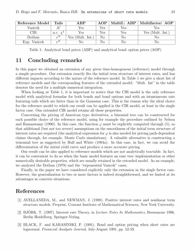
Table 1: Analytical bond prices (ABP) and analytical bond–option prices (AOP)

11 Concluding remarks

In this paper we obtained an extension of any given time-homogenous (reference) model througha simple procedure. Our extension exactly fits the initial term structure of interest rates, and hasdifferent impacts according to the nature of the reference model. In Table 1 we give a short list ofreference models and the corresponding features of the extended model. “Mult. Int” in the tabledenotes the need for a multiple numerical integration.

When looking at Table 1, it is important to notice that the CIR model is the only referencemodel with analytical formulae for both bonds and bond options and with an istantaneous–ratefeaturing tails which are fatter than in the Gaussian case. This is the reason why the ideal choicefor the reference model to which our result can be applied is the CIR model, at least in the singlefactor case. Our extended CIR model retains all these properties.

Concerning the pricing of American type derivatives, a binomial tree can be constructed foreach possible choice of the reference model, using for example the procedure outlined by Nelsonand Ramaswamy (1990). In this case, the function ϕ must be explicitly computed through (5), sothat additional (but not too severe) assumptions on the smoothness of the initial term structure ofinterest rates are required (the analytical expression for ϕ is also needed for pricing path-dependentclaims through, for example, Monte Carlo simulations). A valuable alternative is constructing atrinomial tree as suggested by Hull and White (1994a). In this case, in fact, we can avoid thedifferentiation of the initial yield curve and produce a more accurate pricing.

Our result can be also applied to reference models which are not analytically tractable. In fact,it can be convenient to do so when the basic model features an easy tree–implementation or othernumerically desirable properties, which are usually retained in the extended model. As an example,we analysed the Dothan (1979) and the “exponential Vasicek” cases.

Finally, in the paper we have considered explicitly only the extension in the single factor case.However, the generalization to two or more factors is indeed straightforward, and we hinted at itsadvantages in concrete situations.

References

[1] AVELLANEDA, M., and NEWMAN, J. (1998). Positive interest rates and nonlinear termstructure models. Preprint, Courant Institute of Mathematical Sciences, New York University.

[2] BJORK, T. (1997). Interest rate Theory, in Lecture Notes In Mathematics, Bressanone 1996,Berlin Heidelberg. Springer-Verlag.

[3] BLACK, F. and KARASINSKI, P. (1991). Bond and option pricing when short rates arelognormal. Financial Analysts Journal, July-August 1991, pp .52-59.


[4] BRACE, A., GATAREK, D., and MUSIELA, M. (1997). The market model of interest ratedynamics. Mathematical Finance, Vol. 7, pp. 127–154.

[5] BRIGO, D. , MAURI, G., MERCURIO, F., SARTORELLI, G. (1998). The CIR++ model: Anew extension of the Cox-Ingersoll-Ross model with analytical calibration to bond and optionprices. Internal Report, Banca IMI, Milan.

[6] BRIGO, D. , MERCURIO, F. (2001). A deterministic-shift extension of analytically-tractableand time-homogeneous short-rate models. Finance and Stochastics 5, 369-388.

[7] BRIGO, D. , MERCURIO, F. (2001). Interest Rate Models: Theory and Practice, SpringerVerlag.

[8] CHEN, R, and SCOTT, L. (1992). Pricing interest rate options in a two–factor Cox-Ingersoll-Ross model of the term structure. Review of Financial Studies, 5, pp. 613–636.

[9] COX, J.C., INGERSOLL, J.E. and ROSS, S. (1985). A theory of the term structure of interestrates. Econometrica, 2 pp. 385-407.

[10] COX, J.C., ROSS, S., and RUBINSTEIN, M. (1979). Option Pricing: A Simplified Approach.Journal of Financial Economics, 7 pagg. 229-263, 1979.

[11] DAVIS, M. (1998). A note on the forward measure. Finance and Stochastics, 2, pp. 19-28.

[12] DOTHAN, L.U. (1978). On the term structure of interest rates. Journal Of Financial Eco-nomics 6 pp. 59-69.

[13] DUFFIE, D. (1996). Dynamic Asset Pricing Theory, Second Edition. Academic press, NewYork.

[14] DYBVIG, P.H. (1988). Bond and bond option pricing based on the current term structure,Washington University working paper.

[15] DYBVIG, P.H. (1997). Bond and Bond Option Pricing Based on the Current Term Structure.Mathematics of Derivative Securities, Michael A. H. Dempster and Stanley R. Pliska, eds.Cambridge: Cambridge University Press, pp. 271-293.

[16] HEATH, D., JARROW, R., and MORTON, A. (1992). Bond pricing and the term structure ofinterest rates: a new methodology for contingent claim valuation. Econometrica 1, pp. 77-105.

[17] HULL, J. and WHITE, A. (1990). Pricing interest-rate-derivative securities. The Review OfFinancial Studies, 4 pp. 573-592.

[18] HULL, J. and WHITE, A. (1994a). Numerical procedures for implementing term structuremodels I: single-factor models. The Journal Of Derivatives, Fall 1994 pp. 7-16, 1994.

[19] HULL, J. and WHITE, A. (1994b). Numerical procedures for implementing term structuremodels II: two-factor models. The Journal Of Derivatives, Winter 1994, 37-47, 1994.

[20] JAMSHIDIAN, F. (1988). The one–factor Gaussian interest rate model: Theory and imple-mentation. Working paper, Merril Lynch Capital Markets.


[21] JAMSHIDIAN, F. (1997). LIBOR and swap market models and measures. Finance andStochastics, 4, pp. 293–330.

[22] KIJIMA, M., and NAGAYAMA, I. (1994). Efficient numerical procedures for the HULL–WHITE extended Vasicek model. The journal of financial engineering, 3,4, pp. 275–292.

[23] KLODEN, P.E., and PLATEN, I. (1995). Numerical Solutions of Stochastic Differential Equa-tions. Springer, Berlin Heidelberg New York.

[24] LONGSTAFF, F.A. and SCHWARTZ, E.S. (1992). Interest Rate Volatility and the TermStructure: A Two-Factor General Equilibrium Model. The Journal of Finance 47 , 1259-1282.

[25] MAGHSOODI, Y. (1996). Solution of the Extended CIR Term Structure and Bond OptionValuation. Mathematical Finance, 6, pp. 89–109.

[26] MILTERSEN K.R., SANDMANN K., and SONDERMANN D. (1997). Closed form solutionsfor term structure derivatives with log–normal interest rates. Journal of Finance, 1, pp. 409–430.

[27] MUSIELA, M., and RUTKOWSKI, M. (1997). Continuous–time term structure models: For-ward measure approach. Finance and Stochastics, 4, pp. 261–292.

[28] NELSON, D. B. , and RAMASWAMY, K. (1990). Simple binomial processes as DiffusionApproximations in Financial Models. The Review of Financial Studies, 3, pagg 393–430, 1990.

[29] PELSSER, A.A.J. (1996). Efficient Methods for Valuing and Managing Interest Rate and otherDerivative Securities. PhD Dissertation. Erasmus University Rotterdam, The Netherlands.

[30] RENDLEMAN, R. and BARTTER, B. (1980). The pricing of options on debt securities.Journal of Financial and Quantitative Analysis, 15, pp. 11-24.

[31] ROGERS, L.C.G. (1995). Which model for the term structure of interest rates should onechoose? Mathematical Finance, IMA Volume 65, pp. 93–116, Springer, New York.

[32] SCHMIDT, W.M. (1997). On a general class of non-factor models for the term structure ofinterest rates. Finance and Stochastics, 4, pp. 3–24.

[33] SCOTT, L (1995). The valuation of interest rate derivatives in a multi-factor term-structuremodel with deterministic components. University of Georgia. Working paper.

[34] VASICEK, O.A. (1977). An equilibrium characterization of the term structure. Journal ofFinancial Economics, 5 pp .177-188.

On deterministic–shift extensions of short–rate models · lognormal short–rate model which...

Documents

Transcript of On deterministic–shift extensions of short–rate models · lognormal short–rate model which...