On complete convergence in Marcinkiewicz-Zygmund type SLLN ... fileOn complete convergence in...

IRTG 1792 Discussion Paper 2018-041

On complete convergence in Marcinkiewicz-Zygmund type

SLLN for random variables

Anna Kuczmaszewska * Ji Gao YAN *²

* Lublin University of Technology, Poland *² Soochow University, PR China

This research was supported by the Deutsche Forschungsgemeinschaft through the

International Research Training Group 1792 "High Dimensional Nonstationary Time Series".

http://irtg1792.hu-berlin.de

ISSN 2568-5619

Inte

rnat

iona

l Res

earc

h Tr

aini

ng G

roup

179

2

On complete convergence in Marcinkiewicz-Zygmund type SLLN for random variables1

Anna KuczmaszewskaDepartment of Applied Mathematics, Lublin University of Technology,

Nadbystrzycka 38 D, 20-618 Lublin, Poland

Jigao Yan2

School of Mathematical Sciences, Soochow University, Suzhou 215006, ChinaC.A.S.E. - Center for Applied Statistics and Economics, Humboldt-Universitat zu Berlin,

Spandauer Str. 1, 10178 Berlin, Germany

Abstract: We consider a generalization of Baum-Katz theorem for random vari-

ables satisfying some cover conditions. Consequently, we get the result for many

dependent structure, such as END, %∗-mixing, %−-mixing and ϕ-mixing, etc.

MSC (2010): 60F15.

Keywords: Complete convergence; Marcinkiewicz-Zygmund type SLLN; Extended

negatively dependent; Mixing dependency; Weakly mean bounded.

1 Introduction

In this paper, we consider a sequence Xn, n ≥ 1 of random variables defined onsome probability space (Ω,F , P ). Hsu and Robbins [10] introduced the following conceptof complete convergence. A sequence Xn, n ≥ 1 is said to converge completely to aconstant C if

∞∑n=1

P (|Xn − C| > ε) <∞,

for all ε > 0. For independent and identically distributed (i.i.d., in short) random variablesX,Xn, n ≥ 1, let Sn =

∑nk=1Xk, n ≥ 1 be the partial sums, Hsu and Robbins [10]

proved that Sn/n converge completely to EX, provided DX < ∞. Erdos [8] provedthe converse theorem. This Hsu-Robbins-Erdos’s theorem was generalized in differentways. Katz [13], Baum and Katz [1], and Chow [7] formed the following generalization ofMarcinkiewicz-Zygmund type.

Theorem 1.1 Let X,Xn, n ≥ 1 be a sequence of i.i.d. random variables and letαp ≥ 1, α > 1/2. Then the following statements are equivalent:

(i) E|X|p <∞ and EX = 0 if p ≥ 1;(ii)

∑∞n=1 n

αp−2P (|Sn| > εnα) <∞ for all ε > 0;(iii)

∑∞n=1 n

αp−2P (max1≤i≤n |Si| > εnα) <∞ for all ε > 0;If αp > 1, α > 1/2 the above are also equivalent to(iv)

∑∞n=1 n

αp−2P (supi≥n i−α|Si| > ε) <∞ for all ε > 0.

1Supported by the National Natural Science Foundation of China (No. 11571250)2Correspondence: [email protected](Jigao Yan), Tel: (86)512-65112637, Fax: (86)512-

65222691

1

In many stochastic models, the assumption that random variables are independentis not plausible. Increases in some random variables are often related to decreases inother random variables, so an assumption of dependence is more appropriate than anassumption of independence. One of the important dependence structure is the extendednegatively dependent structure, which was introduced by Liu [18] as follows.

Definition 1.1 Random variables Xk, k = 1, · · · , n are said to be lower extendednegatively dependent (LEND) if there is some M > 0 such that, for all real numbersxk, k = 1, · · · , n,

P

n⋂k=1

(Xk ≤ xk)

≤M

n∏k=1

PXk ≤ xk; (1.1)

they are said to be upper extended negatively dependent (UEND) if there is some M > 0such that, for all real numbers xk, k = 1, · · · , n,

P

n⋂k=1

(Xk > xk)

≤M

n∏k=1

PXk > xk; (1.2)

and they are said to be extended negatively dependent (END) if they are both LEND andUEND. A sequence of infinitely many random variables Xk, k = 1, 2, · · · is said to beLEND/UEND/END if there is some M > 0 such that, for each positive integer n, therandom variables X1, X2, · · · , Xn are LEND/UEND/END, respectively.

In the case M = 1, the formula of END random variables reduces to the notion ofnegatively orthant dependent (NOD, in short) random variables which was introduced byJoag-Dev and Proschan [12]. They also pointed out that negatively associated (NA, inshort) random variables are NOD random variables and then END.

As pointed out in Liu [18], the END structure covers many negative dependence struc-tures and, more interestingly, it covers certain positive dependence structures. Hence,studying the limiting behavior of END random variables is of great significance. Thereare more and more literatures appeared. See, for example, Liu [18] obtained the preciselarge deviations for dependent random variables with heavy tails. Shen [25] presentedsome probability inequalities and gave some applications. Wu et al [33] considered somecomplete moment convergence and mean convergence theorems for the partial sums ofEND random variables. Qiu et al [24], Wang et al [31, 32] and Shen et al [27] investigat-ed some results on complete convergence of END random variables. Chen et al [6], Yan[36, 37] considered the SLLN for END random variables, and so on.

An another group of dependencies is formed by mixing type structures defined byspecial sequences of mixing coefficients. Some of them, however defined in a way that issignificantly different from the negative dependence structures, have many similar prop-erties which allow us to use in consideration methods and tools similar to those used inEND case. In further consideration we will deal with three types of mixing dependencies:%∗-mixing, ϕ-mixing and %−-mixing.

2

Definition 1.2 A sequence of random variable Xn, n ≥ 1 is said to be a %∗-mixingsequence if there exists k ∈ N such that

%∗(k) = supS,T

(sup

X∈L2(FS),Y ∈L2(FT )

cov(X, Y )√V ar(X) · V ar(Y )

)< 1,

where S, T are the finite subsets of positive integers such that dist (S, T ) ≥ k and FW isthe σ-field generated by the random variable Xi, i ∈ W ⊂ N.

Bradley [2] and Miller [19] studied various limit properties of random fields under theassumption %∗(k) → 0, k → ∞. We refer to the results obtained under the condition%∗(k) < 1 for some k ∈ N which is important in estimating the moments of partial andmaxima of partial sums, see Bryc and Smolenski [3] and Peligrad [20]. Peligrad [20], Utevand Peligrad [29] investigated the properties of the maximum of partial sums and usedthem to obtain an invariance principle, Peligrad and Gut [21] presented Rosenthal-typemaximal inequality and rate convergence for the Marcinkiewicz-Zygmund type SLLN,Cai [4] obtained SLLN and complete convergence for random variables with differentdistributions.

Definition 1.3 A sequence of random variables Xn, n ≥ 1 is called to be ϕ-mixing(or uniformly strong mixing) if

ϕ(n) = supk≥1,A∈Fk1 ,P (A)>0,B∈F∞k+n

|P (B|A)− P (B)| → 0 as n→∞,

where Fmn is the σ-field generated by random variables Xn, Xn+1, . . . , Xm.

A concept of ϕ-mixing dependence was introduced independently by Rozanov andVolkonski [23] and Ibragimov [11]. A number of limit theorems for ϕ-mixing randomvariables have been established by many authors. We refer to Wang at al [30] (Rosenthaltype maximal inequality, Hajek-Renyi type inequality, SLLN), Tuyen [28] (SLLN), andChen at al [5] (complete convergence and Marcinkiewicz-Zygmund type SLLN of movingaverages processes) and Kuczmaszewska [16] (complete convergence for NA, %∗-mixingand ϕ-mixing sequences satisfying Petrov’s condition).

Definition 1.4 A sequence Xn, n ≥ 1 is called %−-mixing, if

%−(n) = sup%−(S, T ) : S, T ⊂ N, dist(S, T ) ≥ n → 0, as n→∞,

where

%−(S, T ) = 0 ∨ supcorr(f(Xi, i ∈ S), g(Xj, j ∈ T )),

and the supremum is taken over all coordinatewise increasing real functions f on RS andg on RT .

3

Some results concerning the complete moment convergence, the complete convergenceand strong law of large numbers of Marcinkiewicz-Zygmund type for moving averageprocess generated by %−-mixing seguences one can find in Zhang [38]. We also refer toWang and Lu [34].

Most of results concerning limit theorems are formulated for identically distributedrandom variables. Pruss [22] introduced the following concept of regular cover whichallowed to consider sequences without identical distribution.

Definition 1.5 Let X1, X2, · · · , Xn be random variables, and X be a random vari-able possibly defined on a different probability space. Then, X1, X2, · · · , Xn are said to bea regular cover of (the distribution of ) X provided we have

E(G(X)) =1

n

n∑k=1

E(G(Xk)), (1.3)

for any measurable function G for which both sides make sense.

In this paper, we are interested in generalizations of the Baum-Katz result. Undersome cover condition weaker than (1.3), Kuczmaszewska [14] extended the result to thecase of negatively associated (NA, in short) sequence. They got the following result

Theorem 1.2 (Kuczmaszewska [14]). Let Xn, n ≥ 1 be a sequence of NA randomvariables and X be a random variable possibly defined on a different space satisfying thecondition

1

n

n∑k=1

P (|Xk| > x) = c · P (|X| > x) (1.4)

for all x > 0, all n ≥ 1 and some positive constant c. Let αp > 1 and α > 1/2. Moreover,additionally assume that for p ≥ 1 EXn = 0 for all n ≥ 1. Then the following statementsare equivalent:

(i) E|X|p <∞;(ii)

∑∞n=1 n

αp−2P (max1≤i≤n |Si| > εnα) <∞ for all ε > 0.

Though condition (1.4) is weak in some sense, it remains a strong condition, we evenget the same result for arbitrary random variables with some rough conditions. Gut [9]introduced the following concept of weakly mean dominated

Definition 1.6 We say that the array Xnk, 1 ≤ k ≤ n, n ≥ 1 is weakly meandominated (WMD, in short) by the random variable X if, for some γ > 0,

1

n

n∑k=1

P (|Xnk| > x) ≤ γP (|X| > x), (1.5)

for all x > 0 and all n.

A. Kuczmaszewska and Z. A.Lagodowski [15] introduced another structure which can alsobe used to prove results for non-identically distributed random variables.

4

Definition 1.7 Random variables Xk, k ≥ 1 are weakly mean bounded (WMB, inshort) by random variable X (possibly defined on a different probability space) iff thereexist some constant γ1, γ2 > 0 such that for all x > 0 and n ≥ 1

γ1 · P (|X| > x) ≤ 1

n

n∑k=1

P (|Xk| > x) ≤ γ2 · P (|X| > x). (1.6)

Obviously, if a sequence Xk, k ≥ 1 and a random variable X satisfy WMB condition,they must satisfy WMD ones. The aim of this paper is to consider the analogous gener-alization of the Baum-Katz theorem for a sequence of random variables satisfying WMDor WMB sense and some usual conditions (Marcinkiewicz-Zygmund type inequality andRosenthal type inequality). The main results are provided in Section 2. Some lemmasand the proofs of the main results are presented in Section 3.

As usual, we note that C will be numerical constants whose value are without impor-tance, and, in addition, may change between appearances. I(A) is the indicator functionon the set A. Denote X+ = max(X, 0) and X− = max(−X, 0).

2 Main Results

Before presenting our main results, we first give the following assumptions.Hypothesis. Let Xn, n ≥ 1 be an arbitrary sequence of random variables satisfying

for every θ ≥ 2 and n ≥ 1

E

(∣∣∣∣∣n∑i=1

fi(Xi)

∣∣∣∣∣)θ

≤ C

n∑i=1

E|fi(Xi)|θ +

(n∑i=1

E|fi(Xi)|2)θ/2

(2.1)

and

E

(max1≤k≤n

∣∣∣∣∣k∑i=1

fi(Xi)

∣∣∣∣∣)θ

≤ C logθ n

n∑i=1

E|fi(Xi)|θ +

(n∑i=1

E|fi(Xi)|2)θ/2

, (2.2)

whenever f1, f2, · · · , fn are all nondecreasing (or non-increasing) functions, Efi(Xi) = 0and E|fi(Xi))|θ <∞, for all 1 ≤ i ≤ n.

Remark 2.1 A lot of dependent structures, for example such as ρ∗-mixing, ϕ-mixing, NA, ND, END, etc., satisfy (2.1) and (2.2) in Hypothesis.

Theorem 2.1 Suppose αp > 1, α > 1/2. Let Xn, n ≥ 1 be an arbitrary sequenceof random variables with EXn = 0 for all n ≥ 1 if p > 1 and X be a random variablepossibly defined on a different probability space satisfying (1.5) for all x > 0, all n ≥ 1 andsome positive constant γ. Assume that Xn, n ≥ 1 satisfies the conditions of Hypothesis.Then E|X|p <∞ implies that for all ε > 0

∞∑n=1

nαp−2P

(max1≤k≤n

|Sk| > εnα)<∞, (2.3)

5

and

∞∑n=1

nαp−2P (supi≥n

i−α|Si| > ε) <∞, (2.4)

where Sk =∑k

i=1Xi, 1 ≤ k ≤ n.

The next theorem presents the necessary condition for (2.3) under assumption thatrandom variables Xn, n ≥ 1 and X satisfy WMB condition (1.6).

Example 2.1 We give an example of (1.6). Suppose that P (Xk = 1− 1k) = P (Xk =

2− 1k) = 1/2 for k = 1, 2, · · · , . Then

1

n

n∑k=1

P (|Xk| > x)→

1, 0 ≤ x < 1,

1/2, 1 ≤ x < 2,0, x ≥ 2.

that is, if the mean dominating random variable, X, is such that P (X = 1) = P (X =2) = 1/2, then (1.6) is satisfied.

Theorem 2.2 Suppose αp > 1, α > 1/2. Let Xn, n ≥ 1 be a sequence of randomvariables satisfying (2.1) for θ = 2 and X be a random variable possibly defined on adifferent probability space satisfying (1.6) for all x > 0, all n ≥ 1 and some positiveconstants γ1 and γ2. Then (2.3) implies E|X|p <∞.

As a consequence of Theorem 2.1 and Theorem 2.2 by Lemma 3.2 and Lemma 3.3 weget the following result.

Corollary 2.1 Suppose αp > 1, α > 1/2. Let Xn, n ≥ 1 be a sequence of END,%∗-mixing, %−-mixing or ϕ-mixing random variables and X be a random variable possiblydefined on a different probability space satisfying (1.6) for all x > 0, all n ≥ 1 and somepositive constants γ1 and γ2. Moreover, we assume EXn = 0 for all n ≥ 1 if p > 1and

∑∞n=1 ϕ

12 (n) < ∞ in case of ϕ-mixing sequence. Then the following statments are

equivalent:(i) E|X|p <∞;(ii)

∑∞n=1 n

αp−2P (max1≤i≤n |Si| > εnα) <∞ for all ε > 0.

Remark 2.2 Since END and %−- mixing random variables include NA random vari-ables, our result also holds for NA case.

3 Some Lemmas and Proofs

To prove the main results of the paper, we need the following important lemmas.

Lemma 3.1 (cf.Liu [18]) Let Xn, n ≥ 1 be a sequence of END random variables.For each n ≥ 1, if f1, f2, · · · , fn are all nondecreasing ( or nonincreasing ) functions, thenrandom variables f1(X1), f2(X2), · · ·, fn(Xn) are also END.

6

Lemma 3.2 (cf.Wang et al.[31]) Let p ≥ 2 and Xn, n ≥ 1 be a sequence of ENDrandom variables with EXn = 0 and E|Xn|p < ∞ for each n ≥ 1. Then there exists apositive constant Cp depending only on p such that

E

∣∣∣∣∣n∑i=1

Xi

∣∣∣∣∣p

≤ Cp

n∑i=1

E|Xi|p +

(n∑i=1

E|Xi|2)p/2

, for all n ≥ 1.

and

E

(max1≤j≤n

∣∣∣∣∣j∑i=1

Xi

∣∣∣∣∣p)≤ Cp(log n)p

n∑i=1

E|Xi|p +

(n∑i=1

E|Xi|2)p/2

, for all n ≥ 1.

Lemma 3.3 (cf.Utev and Peligrad[29], Wang and Lu[34], Wang et al.[30]) Letp ≥ 2 and Xn, n ≥ 1 be a sequence of %∗-mixing, %−-mixing or ϕ-mixing randomvariables with EXn = 0 and E|Xn|p < ∞ for each n ≥ 1. Moreover, if Xn, n ≥ 1 are

ϕ-mixing we assume that∑∞

n=1 ϕ12 (n) < ∞. Then there exists a positive constant Cp

depending only on p such that

E

(max1≤j≤n

∣∣∣∣∣j∑i=1

Xi

∣∣∣∣∣p)≤ Cp

n∑i=1

E|Xi|p +

(n∑i=1

E|Xi|2)p/2

, for all n ≥ 1. (3.1)

Lemma 3.4 (cf.Gut [9]) Let Xn, n ≥ 1 be a sequence of random variables sat-isfying a weak dominating condition with mean dominating random variable X, i.e. forsome c > 0

1

n

n∑i=1

P (|Xi| > x) ≤ cP (|X| > x).

Let r > 0 and for some A > 0

X ′i = XiI(|Xi| ≤ A), X ′′i = XiI(|Xi| > A),

X∗i = XiI(|Xi| ≤ A)− AI(Xi < −A) + AI(Xi > A),

and

X ′ = XI(|X| ≤ A), X ′′ = XI(|X| > A),

X∗ = XI(|X| ≤ A)− AI(X < −A) + AI(X > A).

Then(i) if E|X|r <∞, then 1

n

∑ni=1E|Xi|r ≤ CE|X|r;

(ii) 1n

∑ni=1E|X ′i|r ≤ C (E|X ′|r + ArP (|X| > A)) for any A > 0;

(iii) 1n

∑ni=1E|X ′′i |r ≤ CE|X ′′|r for any A > 0;

(iv) 1n

∑ni=1E|X∗i |r ≤ CE|X∗|r for any A > 0.

7

Now, we present the proofs of the main results step by step.Proof of Theorem 2.1. We first take

0 < p′ < p,1

αp< q < 1

such thatα(p− p′) > α(p− p′)q > 1, and p− p′ > 1 if p > 1.

For all 1 ≤ i ≤ n, n ≥ 1, denote that

X(1)ni = −nαqI(Xi < −nαq) +XiI(|Xi| ≤ nαq) + nαqI(Xi > nαq);

X(2)ni = (Xi − nαq)I(Xi > nαq);

X(3)ni = −(Xi + nαq)I(Xi < −nαq).

Then, for every 1 ≤ i ≤ n, n ≥ 1

Xi = X(1)ni +X

(2)ni −X

(3)ni and X

(2)ni ≥ 0, X

(3)ni ≥ 0.

Thus,

∞∑n=1

nαp−2P

(max1≤k≤n

|Sk| > εnα)

≤∞∑n=1

nαp−2P

(max1≤k≤n

∣∣∣∣∣k∑i=1

X(1)ni

∣∣∣∣∣ > εnα/3

)+∞∑n=1

nαp−2P

(max1≤k≤n

∣∣∣∣∣k∑i=1

X(2)ni

∣∣∣∣∣ > εnα/3

)

+∞∑n=1

nαp−2P

(max1≤k≤n

∣∣∣∣∣k∑i=1

X(3)ni

∣∣∣∣∣ > εnα/3

)

=∞∑n=1

nαp−2P

(max1≤k≤n

∣∣∣∣∣k∑i=1

X(1)ni

∣∣∣∣∣ > εnα/3

)+∞∑n=1

nαp−2P

(n∑i=1

X(2)ni > εnα/3

)

+∞∑n=1

nαp−2P

(n∑i=1

X(3)ni > εnα/3

), I1 + I2 + I3. (in say)

To prove (2.3), it suffices to show that Ik <∞, k = 1, 2, 3.For I1, we first prove that

n−α max1≤k≤n

∣∣∣∣∣k∑i=1

EX(1)ni

∣∣∣∣∣→ 0, n→∞. (3.2)

We will do it in three cases.Case I. Let α ≤ 1. Then αp > 1 implies p > 1 and, according to the assumption,

8

EXn = 0, n ≥ 1. It follows from Lemma 3.4 that

n−α max1≤k≤n

∣∣∣∣∣k∑i=1

EX(1)ni

∣∣∣∣∣≤ n−α max

1≤k≤n

∣∣∣∣∣k∑i=1

[EXiI(|Xi| ≤ nαq) + nαqP (|Xi| > nαq)]

∣∣∣∣∣= n−α max

1≤k≤n

∣∣∣∣∣k∑i=1

[EXiI(|Xi| > nαq) + nαqP (|Xi| > nαq)]

∣∣∣∣∣≤ 2n−α

n∑i=1

E|Xi|I(|Xi| > nαq) ≤ 2n1−αE|X|I(|X| > nαq)

≤ Cn1−α · nαq(1−(p−p′))E|X|p−p′ ≤ Cn−[αq(p−p′)−1]−α(1−q) → 0, n→∞.

Case II. Let α > 1 and p > 1. We have

n−α max1≤k≤n

∣∣∣∣∣k∑i=1

EX(1)ni

∣∣∣∣∣ ≤ n−αn∑i=1

[E|Xi|I(|Xi| ≤ nαq) + nαqP (|Xi| > nαq)]

≤ Cn1−α [E|X|I(|X| ≤ nαq) + nαqP (|X| > nαq)] ≤ Cn1−α → 0, n→∞.

Case III. Let α > 1 and p ≤ 1. We have

n−α max1≤k≤n

∣∣∣∣∣k∑i=1

EX(1)ni

∣∣∣∣∣ ≤ n−αn∑i=1

[E|Xi|I(|Xi| ≤ nαq) + nαqP (|Xi| > nαq)]

≤ Cn1−α [E|X|I(|X| ≤ nαq) + nαqP (|X| > nαq)]

≤ Cn1−α · nαq(1−(p−p′))E|X|p−p′ ≤ Cn−[αq(p−p′)−1]−α(1−q) → 0, n→∞.

By (3.2), to prove I1 <∞, we prove only that

I∗1 ,∞∑n=1

nαp−2P

(max1≤k≤n

∣∣∣∣∣k∑i=1

(X

(1)ni − EX

(1)ni

)∣∣∣∣∣ > εnα/6

)<∞. (3.3)

From Hypothesis, for each n ≥ 1, X(1)ni −EX

(1)ni , 1 ≤ i ≤ n remain satisfy the inequalities

in Hypothesis. By αq(p− p′) > 1 and 0 < q < 1, we have for p ≤ 2

α− 1

2− αq

(1− p− p′

2

)> α− 1

2− α

(1− p− p′

2

)=α(p− p′)− 1

2> 0.

By taking

τ > max

2, p,

p− (p− p′)q1− q

,αp− 1

α− 12

,αp− 1

α− 12− αq

(1− p−p′

2

) ,

9

Chebyshev’s inequality and Hypothesis we get

I∗1 ≤ C∞∑n=1

nαp−2−ατE

(max1≤k≤n

∣∣∣∣∣k∑i=1

(X

(1)ni − EX

(1)ni

)∣∣∣∣∣)τ

≤ C∞∑n=1

nαp−2−ατ logτ nn∑i=1

E∣∣∣X(1)

ni

∣∣∣τ + C∞∑n=1

nαp−2−ατ logτ n

(n∑i=1

E∣∣∣X(1)

ni

∣∣∣2)τ/2

, I∗11 + I∗12. (in say)

Again by Hypothesis

I∗11 ≤ C∞∑n=1

nαp−2−ατ logτ nn∑i=1

[E|Xi|τI(|Xi| ≤ nαq) + nαqτP (|Xi| > nαq)]

≤ C∞∑n=1

nαp−1−ατ logτ n · nαq(τ−(p−p′))E|X|p−p′

≤ C∞∑n=1

n−α(1−q)

(τ− p−q(p−p

′)1−q

)−1

logτ n <∞,

and

I∗12 ≤ C∞∑n=1

nαp−2−ατ logτ n

n∑i=1

[E|Xi|2I(|Xi| ≤ nαq) + n2αqP (|Xi| > nαq)

]τ/2

.

Now, we prove I∗12 <∞ in two cases: p > 2 and 0 < p ≤ 2.Let p > 2.

I∗12 ≤ C∞∑n=1

nαp−2−ατ logτ n · nτ/2(EX2

)τ/2 ≤ C∞∑n=1

n−(α− 1

2)

(τ−αp−1

α− 12

)−1

logτ n <∞.

For 0 < p ≤ 2 we have

I∗12 ≤ C∞∑n=1

nαp−2−ατ logτ n ·(nαq(2−(p−p

′)) · n)τ/2 (

E|X|p−p′)τ/2

≤ C

∞∑n=1

nαp−2−τ

[α− 1

2−αq

(1− p−p

′2

)]logτ n <∞.

This ends the proof of I1 <∞. Next for I2 <∞ and each 1 ≤ i ≤ n, n ≥ 1, let

Y(2)ni = (Xi − nαq)I(nαq < Xi ≤ nαq + nα) + nαI(Xi > nαq + nα).

Then Y(2)ni ≥ 0 and

X(2)ni = Y

(2)ni + (Xi − nαq − nα)I(Xi > nαq + nα).

10

Thus,

I2 ≤∞∑n=1

nαp−2P

(n∑i=1

Y(2)ni >

εnα

6

)

+∞∑n=1

nαp−2P

(n∑i=1

(Xi − nαq − nα)I(Xi > nαq + nα) >εnα

6

)

≤∞∑n=1

nαp−2P

(n∑i=1

Y(2)ni >

εnα

6

)+∞∑n=1

nαp−2n∑i=1

P (Xi > nαq + nα)

, I21 + I22. (in say)

By Lemma 3.4,

I22 ≤∞∑n=1

nαp−2n∑i=1

P (|Xi| > nα) ≤ C∞∑n=1

nαp−1P (|X| > nα)

= C∞∑n=1

nαp−1∞∑i=n

P (iα < |X| ≤ (i+ 1)α)

= C∞∑i=1

P (iα < |X| ≤ (i+ 1)α)i∑

n=1

nαp−1

≤ C∞∑i=1

iαpP (iα < |X| ≤ (i+ 1)α) ≤ CE|X|p <∞. (3.4)

Next we prove only that I21 <∞. We first show that

n−αn∑i=1

EY(2)ni → 0, n→∞. (3.5)

If p > 1, then by Lemma 3.4

0 ≤ n−αn∑i=1

EY(2)ni ≤ n−α

n∑i=1

EXiI(Xi > nαq)

≤ n1−αEXI(X > nαq) ≤ n1−α · nαq(1−(p−p′))E|X|p−p′

≤ Cn−[αq(p−p′)−1]−α(1−q) → 0, n→∞.

If 0 < p ≤ 1, then by Lemma 3.4

0 ≤ n−αn∑i=1

EY(2)ni ≤ n−α

n∑i=1

[EXiI(|Xi| ≤ 2nα) + nαP (|Xi| > 2nαq)]

≤ Cn1−α [EXI(|X| ≤ 2nα) + 2nαP (|X| > 2nα) + nαP (|X| > 2nαq)]

≤ Cn1−α[nα(1−(p−p

′)) + nα−αq(p−p′)]

≤ Cn−[αq(p−p′)−1] → 0, n→∞.

11

By (3.5), to prove I21 <∞, it is sufficient to show that

I∗21 =∞∑n=1

nαp−2P

(∣∣∣∣∣n∑i=1

(Y

(2)ni − EY

(2)ni

)∣∣∣∣∣ > εnα

12

)<∞.

We will prove it in two cases: 0 < p < 2 and p ≥ 2.For 0 < p < 2, by Chebyshev’s inequality, Hypothesis, Lemma 3.4 and (3.4) we have

I∗21 ≤ C∞∑n=1

nαp−2−2αE

∣∣∣∣∣n∑i=1

(Y

(2)ni − EY

(2)ni

)∣∣∣∣∣2

≤ C∞∑n=1

nαp−2−2αn∑i=1

E∣∣∣Y (2)ni

∣∣∣2≤ C

∞∑n=1


[E|Xi|2I(nαq < Xi ≤ nαq + nα) + n2αP (|Xi| > nαq + nα)

]≤ C

∞∑n=1


E|Xi|2I(|Xi| ≤ 2nα) + C∞∑n=1

nαp−2n∑i=1

P (|Xi| > nα)

≤ C∞∑n=1

nαp−1−2αE|X|2I(|X| ≤ 2nα) + C∞∑n=1

nαp−1P (|X| > nα)

≤ C∞∑n=1


E|X|2I(2(i− 1)α < |X| ≤ 2iα) + CE|X|p

= C∞∑i=1

E|X|2I(2(i− 1)α < |X| ≤ 2iα)∞∑n=i

nαp−1−2α + CE|X|p

≤ C∞∑i=1

iαp−2αE|X|2I(2(i− 1)α < |X| ≤ 2iα) + CE|X|p

≤ CE|X|p <∞.

Let p ≥ 2. By taking

κ > max

p,αp− 1

α− 12

,2(αp− 1)

α(p− p′)− 1

Chebyshev’s inequality and Hypothesis we have

I∗21 ≤ C∞∑n=1

nαp−2−ακE

∣∣∣∣∣n∑i=1

(Y

(2)ni − EY

(2)ni

)∣∣∣∣∣κ

≤ C∞∑n=1

nαp−2−ακn∑i=1

E∣∣∣Y (2)ni

∣∣∣κ + C∞∑n=1

nαp−2−ακ

(n∑i=1

E∣∣∣Y (2)ni

∣∣∣2)κ/2

, I∗211 + I∗212. (in say)

It is easy to see that

I∗212 ≤ C∞∑n=1

nαp−2−ακ

(n∑i=1

EX2i

)κ/2

≤ C∞∑n=1

nαp−2−ακ+κ2 <∞.

12

On the other hand, by Lemma 3.4 and (3.4) we get

I∗211 ≤ C

∞∑n=1


[E|Xi|κI(nαq < Xi ≤ nα + nαq) + nακP (|Xi| > nα + nαq)]

≤ C∞∑n=1


[E|Xi|κI(|Xi| ≤ 2nα) + nακP (|Xi| > nα)]

≤ C

∞∑n=1

nαp−1−ακ [E|X|κI(|X| ≤ 2nα) + nακP (|X| > nα)]

≤ C∞∑n=1

nαp−1−ακE|X|κI(|X| ≤ 2nα) + CE|X|p

= C∞∑n=1


E|X|κI(2(i− 1)α < |X| ≤ 2iα) + CE|X|p

= C∞∑i=1

E|X|κI(2(i− 1)α < |X| ≤ 2iα)∞∑n=i

nαp−1−ακ + CE|X|p

≤ C∞∑i=1

nαp−ακE|X|κI(2(i− 1)α < |X| ≤ 2iα) + CE|X|p

≤ CE|X|p <∞.

To prove the second thesis of Theorem 2.1 it is enough to show that (2.3) implies (2.4).For 0 < ε < 1 and αp > 1 we have

∞∑n=1

nαp−2P

(supk≥n

k−α|Sk| > ε

)

=∞∑j=1

2j−1∑n=2j−1

nαp−2P

(supk≥n

k−α|Sk| > ε

)≤ C

∞∑j=1

2j(αp−1)P

(sup

k≥2j−1

k−α|Sk| > ε

)

≤ C

∞∑j=1

2j(αp−1)∞∑i=j

P

(max

2i−1≤k<2ik−α|Sk| > ε

)

≤ C∞∑i=1

P

(max


) i∑j=1

2j(αp−1) ≤ C∞∑i=1

2i(αp−1)P

(max


)

≤ C

∞∑i=1

2i(αp−1)P

(max

2i−1≤k<2i|Sk| > ε2(i−1)α

)≤ C

∞∑i=1

2i(αp−1)P

(max1≤k≤2i

|Sk| > ε2−α2iα)

≤ C

∞∑i=1

nαp−2P

(max1≤k≤n

|Sk| > ε2−2αnα)<∞.

This ends the proof of Theorem 2.1.

13

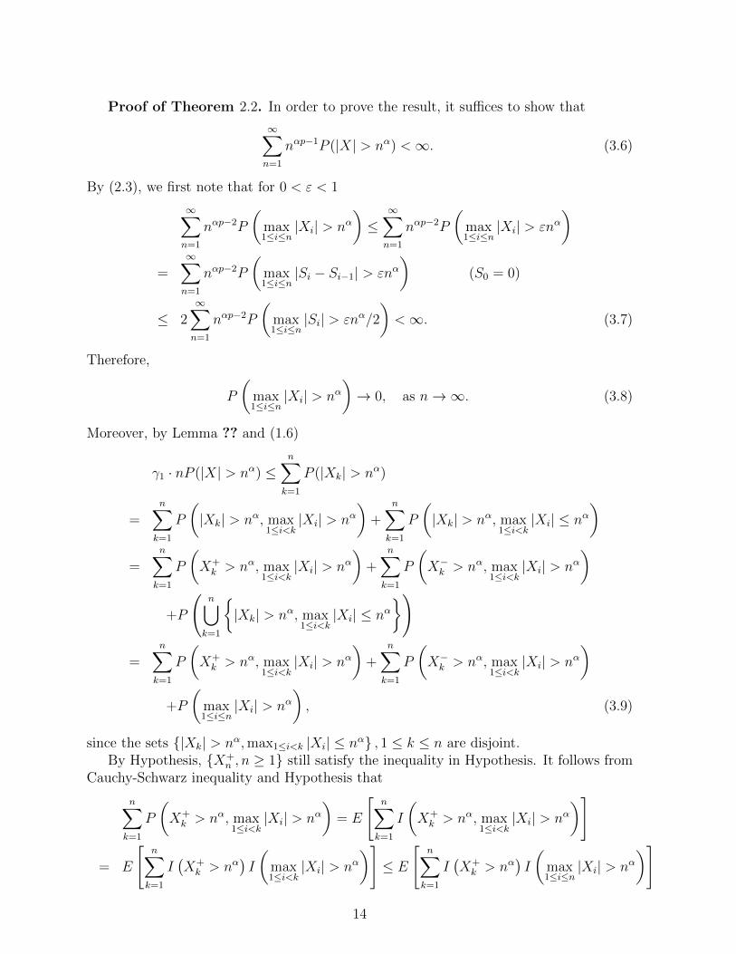
Proof of Theorem 2.2. In order to prove the result, it suffices to show that

∞∑n=1

nαp−1P (|X| > nα) <∞. (3.6)

By (2.3), we first note that for 0 < ε < 1

∞∑n=1

nαp−2P

(max1≤i≤n

|Xi| > nα)≤

∞∑n=1

nαp−2P

(max1≤i≤n

|Xi| > εnα)

=∞∑n=1

nαp−2P

(max1≤i≤n

|Si − Si−1| > εnα)

(S0 = 0)

≤ 2∞∑n=1

nαp−2P

(max1≤i≤n

|Si| > εnα/2

)<∞. (3.7)

Therefore,

P

(max1≤i≤n

|Xi| > nα)→ 0, as n→∞. (3.8)

Moreover, by Lemma ?? and (1.6)

γ1 · nP (|X| > nα) ≤n∑k=1

P (|Xk| > nα)

=n∑k=1

P

(|Xk| > nα, max

1≤i<k|Xi| > nα

)+

n∑k=1

P

(|Xk| > nα, max

1≤i<k|Xi| ≤ nα

)=

n∑k=1

P

(X+k > nα, max

1≤i<k|Xi| > nα

)+

n∑k=1

P

(X−k > nα, max

1≤i<k|Xi| > nα

)

+P

(n⋃k=1

|Xk| > nα, max

1≤i<k|Xi| ≤ nα

)

=n∑k=1

P

(X+k > nα, max

1≤i<k|Xi| > nα

)+

n∑k=1

P

(X−k > nα, max

1≤i<k|Xi| > nα

)+P

(max1≤i≤n

|Xi| > nα), (3.9)

since the sets |Xk| > nα,max1≤i<k |Xi| ≤ nα , 1 ≤ k ≤ n are disjoint.By Hypothesis, X+

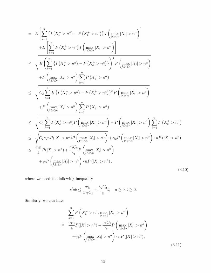
n , n ≥ 1 still satisfy the inequality in Hypothesis. It follows fromCauchy-Schwarz inequality and Hypothesis that

n∑k=1

P

(X+k > nα, max

1≤i<k|Xi| > nα

)= E

[n∑k=1

I

(X+k > nα, max

1≤i<k|Xi| > nα

)]

= E

[n∑k=1

I(X+k > nα

)I

(max1≤i<k

|Xi| > nα)]≤ E

[n∑k=1

I(X+k > nα

)I

(max1≤i≤n

|Xi| > nα)]

14

= E

[n∑k=1

I(X+k > nα

)− P

(X+k > nα

)I

(max1≤i≤n

|Xi| > nα)]

+E

[n∑k=1

P(X+k > nα

)I

(max1≤i≤n

|Xi| > nα)]

≤

√√√√E

(n∑k=1

I(X+k > nα

)− P

(X+k > nα

))2

P

(max1≤i≤n

|Xi| > nα)

+P

(max1≤i≤n

|Xi| > nα) n∑

k=1

P(X+k > nα

)≤

√√√√C2

n∑k=1

EI(X+k > nα

)− P

(X+k > nα

)2P

(max1≤i≤n

|Xi| > nα)

+P

(max1≤i≤n

|Xi| > nα) n∑

k=1

P(X+k > nα

)≤

√√√√C2

n∑k=1

P (X+k > nα)P

(max1≤i≤n

|Xi| > nα)

+ P

(max1≤i≤n

|Xi| > nα) n∑

k=1

P(X+k > nα

)≤

√C2γ2nP (|X| > nα)P

(max1≤i≤n

|Xi| > nα)

+ γ2P

(max1≤i≤n

|Xi| > nα)· nP (|X| > nα)

≤ γ1n

4P (|X| > nα) +

γ2C2

γ1P

(max1≤i≤n

|Xi| > nα)

+γ2P

(max1≤i≤n

|Xi| > nα)· nP (|X| > nα) ,

(3.10)

where we used the following inequality

√ab ≤ aγ1

4γ2C2

+γ2C2

γ1b, a ≥ 0, b ≥ 0.

Similarly, we can have

n∑k=1

P

(X−k > nα, max

1≤i<k|Xi| > nα

)≤ γ1n

4P (|X| > nα) +

γ2C2

γ1P

(max1≤i≤n

|Xi| > nα)

+γ2P

(max1≤i≤n

|Xi| > nα)· nP (|X| > nα) ,

(3.11)

15

Now we see that (3.9), (3.10) and (3.11) lead to

γ1n

2P (|X| > nα) ≤ 2γ2C2 + γ1

γ1P

(max1≤i≤n

|Xi| > nα)

+2γ2nP

(max1≤i≤n

|Xi| > nα)P (|X| > nα)

By (3.8), for sufficiently large n we have

P

(max1≤i≤n

|Xi| > nα)<

γ18γ2

,

and consequently

nP (|X| > nα) ≤ 4(2γ2C2 + γ1)

γ1P

(max1≤i≤n

|Xi| > nα). (3.12)

Relations (3.7) and (3.12) give (3.6) and in conclusion we get the desired conditionE|X|p <∞. This ends the proof of Theorem 2.2.

References

[1] Baum, L.E., Katz, M. Convergence rates in the law of large numbers. Trans. Amer.Math. Soc. 120, 1965, 108-123.

[2] Bradley, R. C. On the spectral density and asymptotic normality of weakly dependentrandom fields. J. of Theor. Probab. vol. 5, no. 2, 1992, 355?73.

[3] Bryc, W., Smolenski, W. Moment conditions for almost sure convergence of weaklycorrelated random variables. Proc. of Amer. Math. Soc. vol. 119, no. 2, 1993, 629?35.

[4] Cai, G.H. Strong law of large numbers for %∗-mixing sequences with different distri-butions Disc. Dynamics in Nat. Soc. vol. 2006, Article ID 27648, 7 pages, 2006

[5] Chen, P., Hu, T., C., Volodin A. Limit behaviour of moving average processes underφ-mixing assumption. Statist. Probab. Lett. 79, 2009, 105-111.

[6] Chen, Y. Chen, A., Ng K., The strong law of large numbers for extended negativelydependent random variables, J. Appl. Probab. 47, 4, 2010, 908C922.

[7] Chow, Y.S. Delayed sums and Borel summability of independent, identically dis-tributed random variables. Bull. Inst. Math. Acad. Sinica1, 1973, 207-220.

[8] Erdos, P. On a theorem of Hsu and Robbins. Ann. Math. Stat. 20, 1949, 286-291.

[9] Gut, A. Complete convergence for arrays. Periodica Math. Hungar. 25, 1992, 51-75.

[10] Hsu, P.L., Robbins, H. Complete convergence and the law of large numbers. Proc.Nat. Acad. Sci. USA 33, 1947, 25-31.

16

[11] Ibragimov, I. A. (1962) Some limit theorems for stationary processes. Theory Probab.Appl. 7 1962, 349-382.

[12] Joag-Dev, K., Proschan, F. Negative association of random variables with applica-tions. The Ann. Stat. 11, 1983, 286-295.

[13] Katz, M. The probability in the tail of a distribution. Ann. Math. Stat. 34, 1963,312-318.

[14] Kuczmaszewska, A. On complete convergence in Marcinkiewicz-Zygmund type SLLNfor negatively associated random variables. Acta. Math. Hungar. 128(1-2), 2010, 116-130.

[15] Kuczmaszewska, A., Lagodowski, Z. A. Convergence rates in the SLLN for someclasses of dependent random fields, J. Math. Anal. Appl. 380, 2011, 571-584.

[16] Kuczmaszewska, Convergence rate in the Petrov SLLN for dependent random vari-ables. Acta. Math. Hungar. 148, 1, 2016, 56-72.

[17] Lagodowski, Z. A. An approach to complete convergence theorems for dependentrandom fields via application of Fuk-Nagaev inequality. J. Math. Anal. Appl. 437,2016, 380-395.

[18] Liu, L. Precise large deviations for dependent random variables with heavy tails.Stat. Probab. Lett. 79, 2009, 1290C1298. doi:10.1016/j.spl.2009.02.001.

[19] Miller, C. Three theorems on %∗-mixing random fields. J. Theor. Probab. 7, 1994,867?82.

[20] Peligrad, M. Maximum of partial sums and an invariance principle for a class of weakdependent random variables. Proc. Amer. Math. Soc. vol. 126, no. 4, 1998, 1181?189.

[21] M. Peligrad, M., Gut,A. Almost-sure results for a class of dependent random vari-ables.J. Theor. Probab. vol. 12, no. 1, 1999, 87?04.

[22] Pruss, A.R. Randomly sampled Riemann sums and complete convergence in the lawof large numbers for a case without identical distribution. Proc. Amer. Math. Soc.124, 1996, 919-929.

[23] Rozanov, Y.A., Volkonski, V.A. Some limit theorems for random function. TheoryProbab. 4, 1959, 186-207.

[24] Qiu, D.H., Chen, P.Y., Antonini, R.G., Volodin, A. On the complete convergence forarrays of rowwise extended negatively dependent random variables. J. Korean Math.Soc. 50, 2, 2013, 379-392.

[25] Shen, A. Probability inequalities for END sequence and their applications, J. Inequal.Appl. 98, 2011, 1-12.

17

[26] Shen, A. Complete convergence for weighted sums of END random variables and itsapplications to nonparametric regression models. J. Nonparametric Stat. 28, 4, 2016,702-715. -

[27] Shen, A., Xue, M., Wang, W. Complete convergence for weighted sums of extend-ed negatively dependent random variables. Communications in Stat.- Theory andMethods 46, 3, 2017, 1433-1444.

[28] Tuyen, D. Q. A strong law for mixing random variables, Periodica Math. Hung. 38,1999, 131-136.

[29] Utev, S., Peligrad, M., Maximal inequalities and an invariance principle for a class ofweakly dependent random variables. J. Theor. Probab. vol. 16, no. 1, 2003, 101?15.

[30] Wang, X., Hu, S., Yang, W.,Shen, Y., On complete convergence for weighted sum-s of ϕ-mixing random variables, J. Ineq. Appl. 2010, Article ID 372390, 13 pagesdoi:10.1155/2010/372390.

[31] Wang, X.J., Li, X.Q., Hu, S.H., Wang, X.H. On complete convergence for an extendednegatively dependent sequence. Communications in Statistics- Theory and Methods43, 2014, 2923-2937.

[32] Wang, X.J., Zheng, L.L., Xu, C., Hu, S.H. Complete consistency for the estimatorof nonparameter regression models based on extended negatively dependent errors.Statistics: A Journal of Theoretical and Applied Stat. 49, 2015, 396-407.

[33] Wu, Y.F., Song, M.Z., Wang, C.H. Complete moment convergence and mean conver-gence for arrays of rowwise extended negatively dependent random variables. The Sci-entific World Journal, Artical ID 478612, 7 pages. 2014, doi: 10.1155/2014/478612.

[34] Wang, J.F., Lu, F. B., Inequalities of maximum of partial sums and weak convergencefor a class of weak dependent random variables. Acta, Math. Sin. 22, 2006, 693-700.

[35] Yan, J.G. The Uniform Convergence and Precise Asymptotics of Generalized Stochas-tic Order Statistics. J. Math. Anal. Appl. 343, 2008, 644-653.

[36] Yan, J.G. Strong Stability of a type of Jamison Weighted Sums for END RandomVariables. J. Korean Math. Soc.54, 3, 2017, 897-907.

[37] Yan, J.G. Almost sure convergence for weighted sums of WNOD random variablesand its applications in nonparametric regression models1. Communications in Stat.-Theory and Methods. 2017.

[38] Zhang, Y., Complete moment convergence for moving average process generated byρ−-mixing random variables. J. Ineq. Appl. 2015, 2015:245, DOI 10.1186/s13660-015-0766-5

18

IRTG 1792 Discussion Paper Series 2018 For a complete list of Discussion Papers published, please visit irtg1792.hu-berlin.de. 001 "Data Driven Value-at-Risk Forecasting using a SVR-GARCH-KDE Hybrid"

by Marius Lux, Wolfgang Karl Härdle and Stefan Lessmann, January 2018.

002 "Nonparametric Variable Selection and Its Application to Additive Models" by Zheng-Hui Feng, Lu Lin, Ruo-Qing Zhu asnd Li-Xing Zhu, January 2018.

003 "Systemic Risk in Global Volatility Spillover Networks: Evidence from Option-implied Volatility Indices " by Zihui Yang and Yinggang Zhou, January 2018.

004 "Pricing Cryptocurrency options: the case of CRIX and Bitcoin" by Cathy YH Chen, Wolfgang Karl Härdle, Ai Jun Hou and Weining Wang, January 2018.

005 "Testing for bubbles in cryptocurrencies with time-varying volatility" by Christian M. Hafner, January 2018.

006 "A Note on Cryptocurrencies and Currency Competition" by Anna Almosova, January 2018.

007 "Knowing me, knowing you: inventor mobility and the formation of technology-oriented alliances" by Stefan Wagner and Martin C. Goossen, February 2018.

008 "A Monetary Model of Blockchain" by Anna Almosova, February 2018. 009 "Deregulated day-ahead electricity markets in Southeast Europe: Price

forecasting and comparative structural analysis" by Antanina Hryshchuk, Stefan Lessmann, February 2018.

010 "How Sensitive are Tail-related Risk Measures in a Contamination Neighbourhood?" by Wolfgang Karl Härdle, Chengxiu Ling, February 2018.

011 "How to Measure a Performance of a Collaborative Research Centre" by Alona Zharova, Janine Tellinger-Rice, Wolfgang Karl Härdle, February 2018.

012 "Targeting customers for profit: An ensemble learning framework to support marketing decision making" by Stefan Lessmann, Kristof Coussement, Koen W. De Bock, Johannes Haupt, February 2018.

013 "Improving Crime Count Forecasts Using Twitter and Taxi Data" by Lara Vomfell, Wolfgang Karl Härdle, Stefan Lessmann, February 2018.

014 "Price Discovery on Bitcoin Markets" by Paolo Pagnottoni, Dirk G. Baur, Thomas Dimpfl, March 2018.

015 "Bitcoin is not the New Gold - A Comparison of Volatility, Correlation, and Portfolio Performance" by Tony Klein, Hien Pham Thu, Thomas Walther, March 2018.

016 "Time-varying Limit Order Book Networks" by Wolfgang Karl Härdle, Shi Chen, Chong Liang, Melanie Schienle, April 2018.

017 "Regularization Approach for NetworkModeling of German EnergyMarket" by Shi Chen, Wolfgang Karl Härdle, Brenda López Cabrera, May 2018.

018 "Adaptive Nonparametric Clustering" by Kirill Efimov, Larisa Adamyan, Vladimir Spokoiny, May 2018.

019 "Lasso, knockoff and Gaussian covariates: a comparison" by Laurie Davies, May 2018.

IRTG 1792, Spandauer Straße 1, D-10178 Berlin http://irtg1792.hu-berlin.de

This research was supported by the Deutsche

Forschungsgemeinschaft through the IRTG 1792.

SFB 649, Spandauer Straße 1, D-10178 Berlin http://sfb649.wiwi.hu-berlin.de


Forschungsgemeinschaft through the SFB 649 "Economic Risk".




IRTG 1792 Discussion Paper Series 2018 For a complete list of Discussion Papers published, please visit irtg1792.hu-berlin.de. 020 "A Regime Shift Model with Nonparametric Switching Mechanism" by

Haiqiang Chen, Yingxing Li, Ming Lin and Yanli Zhu, May 2018. 021 "LASSO-Driven Inference in Time and Space" by Victor Chernozhukov,

Wolfgang K. Härdle, Chen Huang, Weining Wang, June 2018. 022 " Learning from Errors: The case of monetary and fiscal policy regimes"

by Andreas Tryphonides, June 2018. 023 "Textual Sentiment, Option Characteristics, and Stock Return

Predictability" by Cathy Yi-Hsuan Chen, Matthias R. Fengler, Wolfgang Karl Härdle, Yanchu Liu, June 2018.

024 "Bootstrap Confidence Sets For Spectral Projectors Of Sample Covariance" by A. Naumov, V. Spokoiny, V. Ulyanov, June 2018.

025 "Construction of Non-asymptotic Confidence Sets in 2 -Wasserstein Space" by Johannes Ebert, Vladimir Spokoiny, Alexandra Suvorikova, June 2018.

026 "Large ball probabilities, Gaussian comparison and anti-concentration" by Friedrich Götze, Alexey Naumov, Vladimir Spokoiny, Vladimir Ulyanov, June 2018.

027 "Bayesian inference for spectral projectors of covariance matrix" by Igor Silin, Vladimir Spokoiny, June 2018.

028 "Toolbox: Gaussian comparison on Eucledian balls" by Andzhey Koziuk, Vladimir Spokoiny, June 2018.

029 "Pointwise adaptation via stagewise aggregation of local estimates for multiclass classification" by Nikita Puchkin, Vladimir Spokoiny, June 2018.

030 "Gaussian Process Forecast with multidimensional distributional entries" by Francois Bachoc, Alexandra Suvorikova, Jean-Michel Loubes, Vladimir Spokoiny, June 2018.

031 "Instrumental variables regression" by Andzhey Koziuk, Vladimir Spokoiny, June 2018.

032 "Understanding Latent Group Structure of Cryptocurrencies Market: A Dynamic Network Perspective" by Li Guo, Yubo Tao and Wolfgang Karl Härdle, July 2018.

033 "Optimal contracts under competition when uncertainty from adverse selection and moral hazard are present" by Natalie Packham, August 2018.

034 "A factor-model approach for correlation scenarios and correlation stress-testing" by Natalie Packham and Fabian Woebbeking, August 2018.

035 "Correlation Under Stress In Normal Variance Mixture Models" by Michael Kalkbrener and Natalie Packham, August 2018.

036 "Model risk of contingent claims" by Nils Detering and Natalie Packham, August 2018.

037 "Default probabilities and default correlations under stress" by Natalie Packham, Michael Kalkbrener and Ludger Overbeck, August 2018.

038 "Tail-Risk Protection Trading Strategies" by Natalie Packham, Jochen Papenbrock, Peter Schwendner and Fabian Woebbeking, August 2018.

SFB 649, Spandauer Straße 1, D-10178 Berlin

http://sfb649.wiwi.hu-berlin.de

This research was supported by the Deutsche Forschungsgemeinschaft through the SFB 649 "Economic Risk".







SFB 649, Spandauer Straße 1, D-10178 Berlin

http://sfb649.wiwi.hu-berlin.de

This research was supported by the Deutsche Forschungsgemeinschaft through the SFB 649 "Economic Risk".




IRTG 1792 Discussion Paper Series 2018 For a complete list of Discussion Papers published, please visit irtg1792.hu-berlin.de. 039 "Penalized Adaptive Forecasting with Large Information Sets and

Structural Changes" by Lenka Zbonakova, Xinjue Li and Wolfgang Karl Härdle, August 2018.

040 "Complete Convergence and Complete Moment Convergence for Maximal Weighted Sums of Extended Negatively Dependent Random Variables" by Ji Gao YAN, August 2018.

041 "On complete convergence in Marcinkiewicz-Zygmund type SLLN for random variables" by Anna Kuczmaszewska and Ji Gao YAN, August 2018.

SFB 649, Spandauer Straße 1, D-10178 Berlin http://sfb649.wiwi.hu-berlin.de


Forschungsgemeinschaft through the SFB 649 "Economic Risk".







On complete convergence in Marcinkiewicz-Zygmund type SLLN ... fileOn complete convergence in...

Documents

Transcript of On complete convergence in Marcinkiewicz-Zygmund type SLLN ... fileOn complete convergence in...