Oligopoly Theory - John Asker Oligopoly.pdf · Oligopoly Theory We will cover the following topics:...

Oligopoly Theory

This might be revision in parts, but (if so) it is good stuff to be remindedof...

John Asker Industrial Organization January 30, 2019 1 / 1

Oligopoly Theory

We will cover the following topics:

Cournot

Cournot with Sequential Moves

Bertrand

Cournot versus Bertrand

After these basic static models we will examine:

Dynamic oligopoly and Self-enforcing Collusion


Oligopoly TheoryCournot

Cournot wrote in 1838 - well before John Nash!

He proposed an oligopoly-analysis method that is (under many conditions)in fact the Nash equilibrium w.r.t. quantities.

Firms choose. . . production levels.

Version 1: Two-seller game

Cost: TCi (qi ) = ciqi

Demand: p(Q) = a− bQ where Q = q1 + q2



Define a game:

Players: firms.

Action/Strategy set: production levels/quantities.

Payoff function: profits, defined:

π1(q1, q2) = p(q1 + q2)q1 − TC1(q1)

π2(q2, q1) = p(q2 + q1)q2 − TC2(q2)

Now we need an equilibrium concept.



{pc , qc1 , qc2} is a Cournot equilibrium (”Nash-in-quantities” equilibrium) if:

1 a) given q2 = qc2 , qc1 solves maxq1 π1(q1, qc2)

b) given q1 = qc1 , qc2 solves maxq2 π2(q2, qc1)

2 pc = a− b(qc1 + qc2), for pc , qc1 , qc2 ≥ 0

”No firm could increase its profit by changing its output level, given whatother firms produced.”



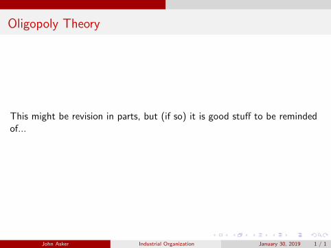
F.O.C. (for firm 1):

∂π1(q1, q2)

∂q1= a− 2bq1 − bq2 − c1 = 0

As always, set marginal revenue (a− 2bq1 − bq2) equal to marginal cost(c1).

How do we know this is a maximum and not a minimum?

∂2π1(q1, q2)

∂(q1)2= −2b < 0 ∀q1, q2



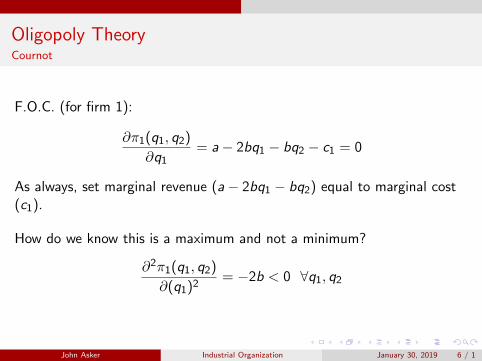
Solve the F.O.C. for q1 ...

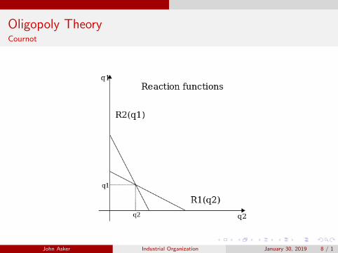
Note: q1 is a function of q2. It is the best-response function, a.k.a.reaction function of firm 1. Call this R1(q2).

q1 = R1(q2) =a− c1

2b− 1

2q2



Note both best-response functions are downward sloping. For each firm: ifthe rival’s output increases, I lower my output level. (i.e., an increase in arival’s output shifts the residual demand facing my firm inward, leading meto produce less.) This feature of ”strategic substitutes”.

Now we can compute Cournot equilibrium output levels.

qc1 =a− 2c1 + c2

3b

qc2 =a− 2c2 + c1

3b

Equilibrium quantity supplied on the market is

Qc = qc1 + qc2 =2a− c1 − c2

3b



We can also find equilibrium price.

pc = a− bQc =a + c1 + c2

3

What are the pay-off functions in equilibrium?

πci = (pc − ci )(qci ) =1

b(qci )2



Version 2: Extending this to N firms.It’s harder to see the reaction functions, but the story is exactly the same.Now each firm maximizes profits according to:

πi (q1, q2, ...qN) = p (Q) qi − TCi (qi )

We would derive the best response function for all N firms. For firm 1,

q1 = R1(q2, ...qN) =a− c1

2b− 1

2

N∑j=2

qj



We need N of these equations. However, if we assume that firms’ marginalcosts are the same (TCi (qi ) = cqi ∀i), it’s a lot easier. Each firm has thesame reaction function, which is

qi = Ri (q−i ) =a− c

2b− 1

2

∑j 6=i

qj



Look at the 2-firm example. When costs (c1 and c2) are the same, outputlevels of the two firms are the same. So, we guess in this case that all theoutput levels (q1, ..., qN) are going to be the same too. If so, denoteqi = q ∀i .

WATCH OUT! We cannot substitute in qi = q before we’ve derived thebest response function. This is a common mistake. Why is it a mistake?

Assuming that qi = q before we take first order conditions implies thatfirm i has control over all firms’ output decisions (the q−i ’s). Here, wesubstitute qi = q into the already-derived best-response functions. We dothis to make the process of solving N equations for N unknowns easier.And, hopefully because we believe the assumption that firms’ costfunctions are truly the same.



Back to the reaction function.

qi = Ri (q−i ) =a− c

2b− 1

2

∑j 6=i

qj

q =

a− c

2b− 1

2(N − 1)q

Thus,

qc =(a− c)

(N + 1)b

Qc =N(a− c)

(N + 1)b

Now it is straightforward to solve for pc (the market price) and πci (profitsfor each firm).



Sanity checks. . .Do we get the monopoly result for N = 1?Do we get the duopoly result for N = 2?What is the Cournot solution for N =∞?

Take the limit as N −→∞ for qc and Qc and pc . They are:

limN→∞

qc = 0

limN→∞

Qc =a− c

blim

N→∞pc = c



Under the assumption of Cournot competition, market supply approachesthe competitive supply as N −→∞.

Note that market supply depends on the slope and intercept of demand,and the (common) marginal cost. Individual firms’ output levels approachzero as N −→∞.



Convince yourself that you can find the equilibrium quantity supplied andprice in the market under the assumption of perfect competition.Simple way: let number of firms = 1, but assume that

∂p

∂Q= 0

and take F.O.C. to find the Q that maximizes profits for the firm underassumptions of perfect competition. This is what we did in the first week.



We have obtained producer surplus under the assumption that N firms in amarket set outputs levels simultaneously according to a”Nash-in-quantities” equilibrium. What about consumer surplus?

We can compute consumer surplus as the area under the demand curve upto the output level that is supplied on the market.

CSc(N) =N2(a− c)2

2b(N + 1)2

Does consumer surplus go up or down as the number of firms increases inthis model?



As for social welfare, we want to compare the sum of firm profits andconsumer surplus as the number of firms increases. (Firms are owned byconsumers in the end...)

We can compute this as a function of the number of firms in the market.

The bottom line: firm profits go down as more firms enter, but consumersurplus goes up, and goes up by more.

W c(N) = CSc(N) + Nπc(N) =

((a− c)2

2b

)(N2 + 2N

N2 + 2N + 1

)The important point:

∂W c(N)

∂N> 0.



Version 3: Different Marginal Costs

We have been assuming that all firms are identical, which impliessymmetric equilibrium outcomes.

Take a look at the results when firms have different levels of marginal cost.

Let marginal cost of firm i be ci . The F.O.C. is only a slight modificationfrom before.

∂πi∂qi

= a− 2bq∗i − b∑i 6=j

q∗j − ci = 0



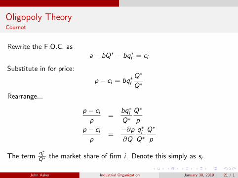
Rewrite the F.O.C. asa− bQ∗ − bq∗i = ci

Substitute in for price:

p − ci = bq∗iQ∗

Q∗

Rearrange...

p − cip

=bq∗iQ∗

Q∗

p

p − cip

=−∂p∂Q

q∗iQ∗

Q∗

p

The termq∗iQ∗ the market share of firm i . Denote this simply as si .



We now have the inverse elasticity rule of Cournot oligopoly:

p − cip

=si−εd


Oligopoly TheoryCournot - Stackelberg

Cournot with Sequential Moves:

We could also think about this in a game where firm 1 moves first, firm 2moves second, etc. We call this a leader-follower market structure, or aStackelberg game.

Keep everything as in the 2-firm cournot model, but assume firm 1 setsquantity (q1) first, then firm 2 sees this qunatity and then chooses itsquantity, q2.



Work backwards: Suppose firm 1 sets output level to q1. What wouldfirm 2 do?

R2(q1) = a−c2b −

12q1

Firm 1 can figure this out. What will Firm 1 do in response?

maxq1 [p(q1 + R2(q1))q1 − cq1]



Firm 1 can figure this out. What will Firm 1 do in response?

maxq1 [p(q1 + R2(q1))q1 − cq1]

What’s different between this profit function and the Cournot profitfunction?



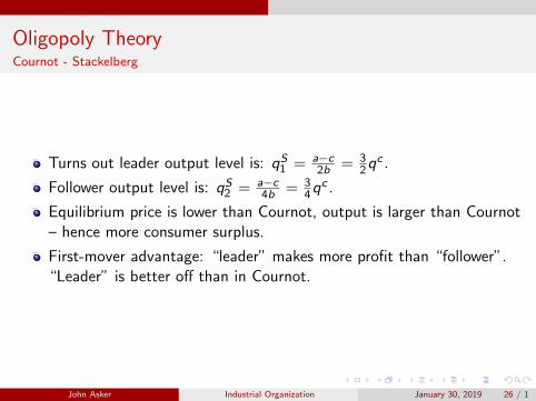
Turns out leader output level is: qS1 = a−c2b = 3

2qc .

Follower output level is: qS2 = a−c4b = 3

4qc .

Equilibrium price is lower than Cournot, output is larger than Cournot– hence more consumer surplus.

First-mover advantage: “leader” makes more profit than “follower”.“Leader” is better off than in Cournot.


Oligopoly TheoryBertrand

When do you think price setting makes more sense than setting quantity?

In general, economists may believe that different assumptions hold fordifferent settings. Then we have to argue about which one is moreconsistent with the data.

Bertrand reviewed Cournot’s work 45 years later.

Go through a two-firm example again. Now firms set prices. We need twoassumptions.

1 Consumers always purchase from the cheapest seller (recall definitionof homogeneous goods).

2 If two sellers charge the same price, consumers are split 50/50.



The second assumption is that demand takes the form:

qi =

0 if pi > pj or pi > aa−p2b if pi = pj = p < aa−pb if pi < min(a, pj)

Equilibrium:{pb1 , p

b2 , q

b1 , q

b2

}is a Bertrand equilibrium (”Nash-in-prices” equilibrium) if:

1 a) given p2 = pb2 , pb1 solves maxp1 π1(p1, pb2 ) = (p1 − c1)q1

b) given p1 = pb1 , pb2 solves maxp2 π2(pb1 , p2) = (p2 − c2)q2

2 q1 and q2 are determined as above.



That is:

“No firm could increase its profit by changing its price, given the price setby the other firm.”



1 If costs are the same, a Bertrand equilibrium is price = marginal cost,with quantity supplied on the market equal to the perfectlycompetitive outcome (equally split between the two firms).

2 If costs differ, (say firm 1 has cost = c1 where c1 < c2), then the firmwith the lower cost charges p1 = c2 − ε, firm 2 sells zero quantity,and firm 1 sells quantity given by qb1 = (a−c2+ε)

b .

Intuition:

If costs are the same, undercutting reduces price to marginal cost. If costsdiffer, undercutting reduces price to ”just below” the cost of the high-costfirm.



Demand

Marginal Cost

P

Q

MC


Oligopoly TheoryBertrand w capacity constraints

(keep the assumption that costs are the same):

Previous results (with no capacity constraints):

1 price competition reduces prices to unit costs

2 firms earn zero profits.

Do we believe these results? Maybe, maybe not.

We might worry about the fact that the number of firms makes nodifference. Undercutting reduces price to marginal cost with only 2 firms.

(Consider the policy implications of this for the anti-trust authorities.)



Edgeworth had the idea that in the short run, firms may be constrained bycapacity that limits their production levels.

Bertrand with capacity constraints:

Consider the following example. There are two hair salons, bothcharging an initial price of $35.

Under the basic Bertrand model (no capacity constraints), Salon-2could take all customers if it set its price at $34.

Suppose initial business is 12 haircuts per day per firm, and that themaximum capacity for either firm is 15 haircuts in a day.

Now the basic Bertrand result of marginal cost pricing won’t arise.



Assume the marginal cost of a haircut is simply c. The regular Bertrandsolution is of course

p1 = p2 = c

π1 = π2 = 0

And the total market output is the same as the competitive level of output

q1 + q2 = QCompetn = a− bp = a− bc

But now add in the capacity constraint (ki ) with the following features:

ki < QCompetn

ki >1

2(QCompetn)



If p2 > p1 = c , firm 2 loses some customers, but not all of them, becausefirm 1 cannot serve the entire residual demand.=⇒ π2 > 0 for p2 = p1 + ε

In other words, there exists a unilateral profitable deviation fromp1 = p2 = c .

p1 = p2 = c is not a Nash equilibrium of the Bertrand game with capacityconstraints (of the type described above).

In order the determine the Nash equilibrium of the price-setting game withcapacity constraints, we can consider a two-stage game:

1 Firms invest in (choose) capacities; then

2 Firms choose prices



Example:

Let c = 0, p = 1− Q, for Q = q1 + q2.

Capacity of each firm: k1, k2

Capacity has been acquired at unit cost c0 ∈ [ 34 , 1]

Claim 1: Firms won’t invest in capacities above 13

Proof 1: Monopoly profit is 14 . Net profit is negative for ki >

13 .



Let c = 0, p = 1− Q, for Q = q1 + q2.

Capacity of each firm: k1, k2

Capacity has been acquired at unit cost c0 ∈ [ 34, 1]

Claim 2: If ki ≤ 13 , both firms charging p∗ = 1− (k1 + k2) is an

equilibrium, and this equilibrium is unique

Proof: Suppose firm 2 is charging p∗ and has capacity k2. Whatshould firm 1 do?

Can firm 1 lower price? No, because at p∗, both firms are at capacity,so there’s no use in lowering price.

Can firm 1 raise price? Assume she charges p1 ≥ p∗. Let q1 be thequantity that firm 1 sells at this high price. Then profit is(1− q1 − k2)q1. Derivative is 1− 2q1 − k2. This is greater than 0when q1 = k1 since ki ≤ 1

3 , i.e. lowering quantity, or equivalently,raising price is not profitable.



Claim 3: Given Claim 2, it is optimal for firms to set capacities equalto Cournot levels in the first stage.

Proof 3, step 1: In second stage, p∗ = 1− (k1 + k2).

Proof 3, step 2: Hence, firm 1’s profit function is:(1− k1 − k2)k1 − c0k1, with derivative (or best-response function),1− 2k1 − k2 − c0. Hence, k1 = k2 = 1−c0

3 .

CRUCIAL ASSUMPTION: setting capacities above 13 is not

profitable. This was due to the high investment costs.



We made this rather problematic assumption since it turns out that iffirms build capacity above the Cournot level, then there is no purestrategy equilibrium in the second stage. Mixed strategies are prettytough to derive; you can look at Kreps and Scheinkman (1983) for afull derivation.

Main message of the above model, however, is that capacityconstraints can soften Bertrand competition.

Sometimes regulation/government can help firms ”coordinate” oncapacity limits. Example: zoning laws in communities prevent largestores from being set up.


Oligopoly TheoryOverview

Comparison of Equilibrium in Models Covered So Far:

Monopoly (M), Cournot (C), Stackelberg

CSM < CSC < CSS < CSPC

PSM > PSC > PSS > PSPC = 0

DWLM > DWLC > DWLS > DWLPC = 0


Price DiscriminationSecond Degree

Problems and Examples: See Handout


Oligopoly Theory - John Asker Oligopoly.pdf · Oligopoly Theory We will cover the following topics:...

Documents

Transcript of Oligopoly Theory - John Asker Oligopoly.pdf · Oligopoly Theory We will cover the following topics:...