Dynamic Bertrand Oligopoly

Andrew Ledvina∗ Ronnie Sircar†

April 8, 2010; revised June 8, 2010

Abstract

We study continuous time Bertrand oligopolies in which a small number of firms producingsimilar goods compete with one another by setting prices. We first analyze a static version ofthis game in order to better understand the strategies played in the dynamic setting. Within thestatic game, we characterize the Nash equilibrium when there are N players with heterogeneouscosts. In the dynamic game with uncertain market demand, firms of different sizes have differentlifetime capacities which deplete over time according to the market demand for their good. Wesetup the nonzero-sum stochastic differential game and its associated system of HJB partialdifferential equations in the case of linear demand functions. We characterize certain qualitativefeatures of the game using an asymptotic approximation in the limit of small competition. Theequilibrium of the game is further studied using numerical solutions. We find that consumersbenefit the most when a market is structured with many firms of the same relative size producinghighly substitutable goods. However, a large degree of substitutability does not always lead tolarge drops in price, for example when two firms have a large difference in their size.

1 Introduction

We study competitive markets with a small number of players in which firms use price as theirstrategic variable in an uncertain demand environment. These are known as Bertrand oligopolies.The firms are selling differentiated but substitutable goods. Many products, for instance consumergoods, are sold in markets that fit this structure. An example might be Pepsi and Coca-Cola inthe market for soft drinks. Oil, coal and natural gas are commodities that can be substituted forone another for energy production, but which have different prices per unit of energy produced.

In this paper, we analyze price setting competition in the case of differentiated goods, andin continuous time under randomly fluctuating demands. These are nonzero-sum stochastic dif-ferential games that may be characterized by systems of Hamilton-Jacobi-Bellman PDEs. Thelarge literature on oligopolistic competition deals primarily with the static problem, and we referto Friedman [18] and Vives [27] for background and references. Cournot [11] provided the firstanalysis of an oligopoly where firms’ strategic interactions are taken into account. He assumedthat firms compete using quantity as their strategic variable and then take prices as determinedby the market through an inverse demand function, that is, a mapping from quantity to price. Ina scathing review of Cournot’s paper, Bertrand [7] argued that firms compete using price as theirstrategic variable and then produce to clear the market demand arising from a demand function,

∗ORFE Department, Princeton University, Sherrerd Hall, Princeton NJ 08544; aledvina@princeton.edu. Workpartially supported by NSF grant DMS-0739195.†ORFE Department, Princeton University, Sherrerd Hall, Princeton NJ 08544; sircar@princeton.edu. Work par-

tially supported by NSF grant DMS-0807440.

1

that is, a mapping from price to quantity. In actuality, some markets may be better modeled asCournot, and others as Bertrand, and we do not enter that debate here.

In both these original models, however, the goods were homogeneous, that is perfectly substi-tutable. This means that the only difference between the firms is the price they set or the quantitythey produce. In the price setting game, this induces the behavior that, if the prices betweentwo goods are not equal, consumers will only purchase the lower priced good. Here, we do notassume goods are perfectly substitutable, and therefore, if firms have prices that differ, they mayall still receive some demand from the market. Models of product differentiation originated withHotelling [23] and Chamberlin [10], and were extended by d’Aspremont et al. [12], among others.See Friedman [18, Chapter 3] for an excellent discussion.

Most of the continuous-time models are in a linear-quadratic (LQ) set-up, which has convenientanalytical properties. We refer to Engwerda [15] for details, and Hamadene [20] for an approachvia BSDEs. Jun and Vives [24] work within the context of a differential game of a duopoly withdifferentiated products. Their general model allows for either Cournot or Bertrand competition inwhich the players control the rate of change of the rate of production or price, respectively, in theLQ setting.

There has been much recent interest in other types of stochastic differential games. We mention,for example, Lasry and Lions [25], who consider Mean Field Games in which there are a large numberof players and competition is felt only through an average of one’s competitors, with each player’simpact on the average being negligible. Bensoussan et al. [6] study leader-follower differentialgames in real options problems. Ekeland and Pirvu [14] and Bjork and Murgoci [9] analyze time-inconsistent control problems which can be viewed as games against one’s future self. Energymarkets in which a small number of firms control supply can be viewed as Cournot oligopolies andthey are analyzed in the context of exhaustible resources in Harris et al. [22].

The state variable of the firms in our model is their remaining lifetime capacity. This is aquantity whose value at time zero represents all of the possible production a firm can undertakeover its lifetime before it goes out of business. The primary reason for this choice is that it isa natural way to capture the notion of relative sizes of firms. A firm with a very large lifetimecapacity is a major market participant whose decisions greatly affect the prevailing price in themarket. A firm with a very small lifetime capacity has very little market power. Here, we analyzethe effect that participant size has on Bertrand markets over time. For producers of consumergoods, the lifetime capacities could be proxied by past volume of sales projected forward into theexpected lifetime of the firm. In the case of exhaustible resources, the state variables would beestimates of remaining oil, coal or natural gas reserves, for instance.

In Section 2, we set up the static version of our price setting game and prove the existenceand uniqueness of a Nash equilibrium. The resulting equilibrium price functions are inputs forSection 3 where we present the dynamic Bertrand game. We characterize the price strategies of thefirms using the solution to a system of coupled nonlinear PDEs. We analyze in detail the problemof a duopoly with linear demand functions and the related monopoly problem. Analytically, weobtain an asymptotic expansion in powers of a parameter that represents the extent of competitionbetween the firms in a deterministic game. In Section 4, we present the numerical solution of oursystem of PDEs that allows us to characterize the price strategies and resulting demands of firmsin the stochastic game. Finally, in Section 5, we conclude and discuss further lines of research.

2

2 Static Bertrand Game

The main purpose of this paper is to analyze a dynamic price setting game in continuous time.In order to fully understand this game, we first analyze a static version of the game and proveexistence and uniqueness of a Nash equilibrium. This is used in establishing the system of HJBPDEs of the dynamic game in the next section.

We assume a market with N firms where each firm uses price as a strategic variable in noncoop-erative competition with the remaining firms. Associated to each firm i ∈ {1, . . . , N} is a variablepi ∈ R+ that represents the price at which firm i offers its good for sale to the market. We denoteby p the vector of prices whose ith element is pi.

2.1 Systems of Demand

Given prices of the firms, we specify the resulting market demands for each firm’s good. For eachfirm i ∈ {1, . . . , N}, there exists a demand function DN

i (p1, p2, . . . , pN ) : RN+ → R. We first statesome natural properties of these demand functions.

Assumption 2.1 (Properties of Demand Functions). For all i = 1, . . . , N , DNi is smooth in all

variables, and

DNN (0, . . . , 0) > 0,

∂DNi

∂pi< 0, and

∂DNi

∂pj> 0 for i 6= j.

We further assume that firms are distinguished only by the prices they set.

Assumption 2.2 (Exchangeability of Firms). For fixed p1, . . . , pN and all i, j ∈ {1, . . . , N},

DNi (p1, . . . , pi, . . . , pj , . . . , pN ) = DN

j (p1, . . . , pj , . . . , pi, . . . , pN ) .

This implies that the demand function is invariant under permutations of the other firms’ prices.That is, for any j, k ∈ {1, . . . , N} \ {i}, we have

DNi (p1, . . . , pi, . . . , pj , . . . , pk . . . , pN ) = DN

i (p1, . . . , pi, . . . , pk, . . . , pj . . . , pN ) .

Smoothness of these functions is for convenience, and, naturally, the market has positive demandif the prices are low enough. The key assumption in the above is that demand for an individualfirm is decreasing in the firm’s own price and increasing in the price of their rivals. This assumptionimplies that we only deal with substitute goods. A classical example is Coca-Cola versus Pepsi.However, such goods can also be of different kinds and thus not directly replaceable, yet they stillexhibit substitutability. For example, an iPod and a compact disc. One cannot directly replace theother, but we expect a drop in the price of iPods to cause a drop in the demand for compact discs.Contrary to this type of good, there are goods known as complementary goods, such as hot dogsand hot dog buns, but we do not consider those kinds of competition here.

We now make additional convenient assumptions.

Assumption 2.3 (Finite Choke Price). Fix a firm i ∈ {1, . . . , N}. For any fixed set of pricesp−i , (p1, . . . , pi−1, pi+1, . . . , pN ), we assume there exists a “choke price”, pi (p−i) <∞, such that

DNi (p1, . . . , pi−1, pi, pi+1, . . . , pN ) = 0. (1)

Note that this “choke price” is unique by Assumption 2.1 because ∂DNi /∂pi < 0. This price is

also positive by the same assumption and Assumption 2.2 because DNN (0, . . . , 0) = DN

i (0, . . . , 0) >DNi (0, . . . , 0, p (0) , 0, . . . , 0) = 0. This implies pi (0) > 0.

3

Remark 2.1. For example, suppose each firm’s demand depends on its rivals’ prices only through

their sum: DNi = f

(pi,∑

j 6=i pj

)where f(x, y) : R+ × R+ → R is a smooth function which is

increasing in y, decreasing in x, and such that there exists a solution x to f(x, y) = 0 for every y.Then, it is easy to see that this demand system satisfies Assumptions 2.1, 2.2 and 2.3.

The actual demand that each firm faces cannot be negative as the firms are suppliers. For afixed price vector p, we define Di(p), without the superscript, as the actual demand firm i receivesin the market. Suppose first, for simplicity, that p1 ≤ p2 ≤ · · · ≤ pN . If this is not the case, thenwe can re-order the firms, carry out the following procedure, and then return them to their originalorder once their demands have been determined. We next show that if prices are ordered, then thissame ordering carries over to the demands.

Proposition 2.1 (Price order implies demand order). Fix a vector of prices p. Suppose they areordered such that p1 ≤ p2 ≤ · · · ≤ pN . Then,

DN1 (p1, . . . , pN ) ≥ DN

2 (p1, . . . , pN ) ≥ · · · ≥ DNN (p1, . . . , pN ) .

Proof. Using the ordering of the prices, the properties of the derivatives of the demand functions,and Assumption 2.2, we have

DNN (p1, . . . , pN−2, pN−1, pN ) = DN

N−1 (p1, . . . , pN−2, pN , pN−1)

≤ DNN−1 (p1, . . . , pN−2, pN−1, pN−1)

≤ DNN−1 (p1, . . . , pN−2, pN−1, pN ) .

The result then follows for all DNi by applying the same procedure. �

To determine the actual demand Di(p), we begin with the demand function DNN (p1, p2, . . . , pN ).

If DNN (p) ≥ 0, then it must be the case that DN

i (p) ≥ 0 for all i = 1, . . . , N by Proposition 2.1.The actual demand that each firm faces is DN

i (p). Hence,

Di(p) = DNi (p) for all i = 1, . . . , N,

and all the demands are determined. Otherwise, if DNN (p) < 0, then the price pN is too high

relative to the preference structure of the market to make any sales in the market. Thus, this firmwill receive no demand from the market and the demand of the remaining firms must reflect thisfact. The demand for firm N is set to zero, DN (p) = 0, and the demand for the remaining firms isdetermined by considering their residual demand functions, which we now define.

Let us consider the general case of residual demand for n firms when all firms i > n receive zerodemand at the current set of prices.

Definition 2.1 (Consistency of Demand). For each n ∈ [1, N − 1], we define the n-firm system ofdemand functions from the (n+ 1)-firm system of demand functions through

Dni (p1, p2, . . . , pn) = Dn+1

i (p1, p2, . . . , pn, pn+1) for i = 1, . . . , n,

where pn+1 (p1, . . . , pn) is defined by Dn+1n+1 (p1, . . . , pn, pn+1) = 0.

Definition 2.1 encapsulates that, if firm n+ 1 sets price so high that Dn+1n+1(p) < 0, demands for

firms i < n+ 1 are consistently adjusted as if firm n+ 1 set price pn+1 that realizes it exactly zerodemand. This will give rise to actual demands which are continuous as a firm raises its price throughthe level at which it receives zero demand, and the market effectively has one less player. We shall

4

see in Remark 2.3 that a common way of generating demand systems through a representativeconsumer’s utility maximization problem yields a demand system with this consistency property.

In Definition 2.1, we do not necessarily know that pn+1 exists for all n. We shall prove thatthey do exist in Proposition 2.2, but first we need to make one additional assumption.

Assumption 2.4. For all n ∈ [1, N − 1] and all i = 1, . . . , n, we assume∂Dn

i∂pi

< 0.

We will see in Propositions 2.2 and 2.3 that the other natural properties of Assumptions 2.1,2.2 and 2.3 are inherited by the lower level demand functions. However, it is necessary to assumethat lower level demand functions are decreasing in each player’s own price.

Proposition 2.2. For each n ∈ [1, N−1], there exists a finite “choke price” pn+1(p1, . . . , pn) where

Dn+1n+1 (p1, . . . , pn, pn+1) = 0.

Proof. See Appendix A. �

Proposition 2.3 (Inherited Demand Properties). The functions Dni , as defined in Definition 2.1,

are smooth in all variables, and∂Dn

i∂pj

> 0 for i 6= j, and i = 1, . . . , n.

The functions Dni also inherit the symmetry of the functions DN

i from Assumption 2.2. Fur-thermore, they inherit the ordering of demand shown in Proposition 2.1. That is, for a fixed vectorof prices p, ordered such that p1 ≤ p2 ≤ · · · ≤ pN , we have for any 1 ≤ n ≤ N

Dn1 (p1, . . . , pn) ≥ Dn

2 (p1, . . . , pn) ≥ · · · ≥ Dnn (p1, . . . , pn) .

Proof. The smoothness of the functions Dni clearly comes directly from that of DN

i . Furthermore,the symmetry of these functions is also clearly inherited. To show the positive transverse derivative,we simply compute. We show only at the level N − 1; for all n ∈ [1, N − 1], the property will followin the exact same way from the function at the level n+ 1 using Assumption 2.4. We first take thederivative of Eqn. (1) with respect to pj for j 6= N , which gives

∂pN∂pj

= −∂DN

N /∂pj

∂DNN /∂pN

> 0, because∂DN

N

∂pj> 0 and

∂DNN

∂pN< 0.

Then, for i = 1, . . . , N − 1 and j ∈ {1, . . . , N − 1} \ {i}, we have

∂DN−1i

∂pj=∂DN

i

∂pj+∂DN

i

∂pN

∂pN∂pj

.

This is positive because of Assumption 2.1 and because ∂pN∂pj

> 0 for any j 6= N . With these

properties, the ordering of demands follows by applying the exact same proof as Proposition 2.1. �

We can now specify completely the demand function that each firm faces for a given set ofprices.

Definition 2.2. (Actual Demands) Given an ordered price vector p:

• If DNN (p) ≥ 0, then Di(p) = DN

i (p) for all i = 1, . . . , N .

5

• Otherwise, find n ∈ {1, . . . , N − 1} such that

Dn+1n+1 (p1, . . . , pn, pn+1) < 0, and Dn

n (p1, . . . , pn) ≥ 0.

For such an n, the actual demands of firms n + 1, . . . , N are equal to zero, and Dni give the

actual demands for each firm i ∈ {1, . . . , n}:

Di(p) =

{Dni (p1, p2, . . . , pn) for i = 1, . . . , n

0 for i = n+ 1, . . . , N

• If no such n exists, then Di(p) = 0 for all i = 1, . . . , N .

2.2 Example: Linear Demand

We present demand functions that are affine in the prices of all firms. This is the demand structurewe will use in the dynamic game of the following sections. For fixed N , we start with positiveparameters A,B,C such that B > (N − 1)C. This latter condition on the parameters will bejustified in what follows. With these parameters, we define

DNi (p1, . . . , pN ) , A−Bpi + C

∑j 6=i

pj , for i = 1, . . . , N. (2)

Notice that DNN (0, . . . , 0) = A > 0, and DN

i is of the form given in Remark 2.1. Therefore thedemand functions satisfy Assumptions 2.1, 2.2 and 2.3.

Proposition 2.4. For each n ∈ [1, N − 1], we have

Dni (p1, . . . , pn) = an − bnpi + cn

∑j 6=ij≤n

pj , for i = 1, . . . , n, (3)

where, for 2 ≤ n ≤ N ,

an−1 = an

(1 +

cnbn

), bn−1 = bn

(1− c2n

b2n

), cn−1 = cn

(1 +

cnbn

), (4)

with aN = A, bN = B and cN = C.

Proof. Using Definition 2.1, we solve for the choke price pN by setting DNN in Eqn. (2) to zero and

solving for pN . This results in pN = B−1(A+ C

∑N−1i=1 pi

). Substituting into Eqn. (2) we obtain,

for i = 1, . . . , N − 1,

DN−1i (p1, . . . , pN−1) = A

(1 +

C

B

)−B

(1− C2

B2

)pi + C

(1 +

C

B

) ∑j 6=i

j≤N−1

pj ,

which establishes Eqn. (4) for n = N . We can repeat this procedure for 1 ≤ n ≤ N − 1, where wefind pn+1 = b−1n+1 (an+1 + cn+1

∑ni=1 pi), and this results in the demand system at the level n being

given by Eqn. (3) with the recursively defined parameters given in Eqn. (4). �

6

Proposition 2.5. The explicit solution of the recursion (4) is given by

an =α

β + (n− 1)γ, bn =

β + (n− 2)γ

(β + (n− 1)γ)(β − γ), cn =

γ

(β + (n− 1)γ)(β − γ), (5)

where we define

γ =C

(B − (N − 1)C) (B + C), α = γ ·A ·

(B

C+ 1

), β = γ ·

(B

C− (N − 2)

). (6)

Proof. Simple algebra shows that the expressions in Eqn. (5) satisfy the recursions in Eqn. (4). Allthat remains to show is that an, bn, cn are positive and well-defined. By examination of Eqn. (5),this will be the case provided α, β, γ are positive, and β > γ because of the denominator in thelast two expressions in Eqn. (5). We see from the first expression in Eqn. (6) that α > 0 if γ > 0.Furthermore, we have that β > γ, and therefore β > 0 if γ > 0 and if B > (N − 1)C. This isexactly the condition we assumed above on the parameters B and C. Therefore, we need only showthat γ > 0, but this again will be true if B > (N − 1)C. Hence, we have that an, bn, cn are positivefor all n. �

Remark 2.2. Note that Assumption 2.4 is satisfied by the demand functions in Eqn. (3) because∂Dn

i∂pi

= −bn < 0, for all n ≤ N and i ≤ n.

Remark 2.3 (Generating Demand Systems). One can generate demand systems that satisfy ourassumptions by starting with a utility function and using the utility maximization problem of a rep-resentative consumer. Let U(q) : RN+ → R be a smooth and strictly concave utility function, whereq is a vector representing quantities of the different products. We assume that a representativeconsumer solves the problem of maximizing utility of consumption minus the cost of that consump-tion: maxq U(q) − pq. One then obtains inverse demands from the first order conditions of thismaximization problem p = ∇U . The Jacobian of the inverse demand system equals the Hessian ofU , which implies the system is invertible. We obtain the direct demand system {DN

i } by invertingthis system for quantity as a function of price. Concavity of U implies ∂DN

i /∂pi < 0, but we cannottell directly from U if ∂DN

i /∂pj ≥ 0 holds for j 6= i. Therefore, an additional assumption mustbe made at the level of the demand functions in order to model substitute goods. However, theconsistency property in Definition 2.1 is guaranteed. Suppose firm N is removed from the utilityfunction, then the demand functions {DN−1

i } derived this way, inverting ∇U after setting qN = 0,are consistent with the {DN

i }, and similarly for the lower level demand functions {Dni }. The linear

system of demand introduced in Section 2.2 can be obtained by using the quadratic utility function

U(q) = α

N∑i=1

qi −1

2

β N∑i=1

q2i + γ∑∑i 6=j

qiqj

.

While it is not necessary to assume that demand is derived from utility, it can be shown that,under some mild conditions, given a system of demand, there exist preferences that rationalize thatdemand, which result in a utility function consistent with that demand system. See Mas-Colellet al. [26, Section 3.H] for more details.

2.3 Nash Equilibrium

We now analyze the static Bertrand game. Each firm i ∈ {1, . . . , N} has an associated constantmarginal cost, denoted by si. We denote by s the vector of costs with ith element equal to si. Each

7

firm chooses its price to maximize profit in a non-cooperative manner, but they must do so whiletaking into account the actions of all other firms. Firms choose prices to maximize profit in thesense of Nash equilibrium. The profit function Πi : RN × R→ R+ for firm i is given by

Πi (p1, p2, . . . , pN , si) , Di(p) · (pi − si) , (7)

where Di(p) was defined using the procedure in Section 2.1.In order to simplify exposition, we assume, possibly after a suitable relabeling, that firms are

ordered by costs: 0 ≤ s1 ≤ s2 ≤ · · · ≤ sN .

Definition 2.3. A vector of prices p? = (p?1, p?2, . . . , p

?N ), is a Nash equilibrium of the Bertrand

game ifp?i = si whenever Di (p?) = 0, (8)

andp?i = arg max

p≥siΠi

(p?1, p

?2, . . . , p

?i−1, p, p

?i+1, . . . , p

?N , si

)(9)

for all i = 1, . . . , N .

Eqn. (9) says the Nash equilibrium is a fixed point of best-responses. Eqn. (8) says that whenevera firm receives zero demand in equilibrium, it sets its price equal to cost, which is a best-response,meaning it satisfies Eqn. (9). This makes the best-response p?i a well-defined function.

In the game with heterogeneous costs, some firms may receive zero demand, and so we first con-sider subgames which, for n = 1, . . . , N , involve only the first n players. Let p?,n =

(p?,n1 , . . . , p?,nn ,

sn+1, . . . , sN ), where the first n components solve the Nash equilibrium problem with profit func-tions Πn

i (p1, . . . , pn) = Dni (p1, . . . , pn) · (pi−si) and Dn

i , introduced in Definition 2.1, is the demandfunction for the n-player game. In other words,

p?,ni = arg maxp≥0

Πni

(p?,n1 , p?,n2 , . . . , p?,ni−1, p, p

?,ni+1, . . . , p

?,nn

), i = 1, . . . , n. (10)

Assumption 2.5. We assume that, for each n = 1, . . . , N , there exists a unique solution to thesystem of maximization problems in Eqn. (10).

Sufficient conditions for the existence of a unique best-response function for each player areexistence of a unique solution to the first-order conditions:

∂Di

∂pi(p?,n)

(p?,ni − si

)+Di(p

?,n) = 0, i = 1, . . . , n, (11)

and strict concavity of Πni as a function of pi. It is straightforward to show that the latter is implied

if we adopt the assumption thatDni (p1, . . . , pn) is concave as a function of pi; some weaker conditions

on the Dni are discussed in Vives [27, Chapter 6], but we do not pursue those here. Finally, for a

unique intersection of the best-reponse functions, hence a unique solution to Eqn. (10), a well-knownsufficient condition is diagonal dominance of the Hessian of Πn

i :

∂2Πni

∂p2i+∑j 6=i

∣∣∣∣ ∂2Πni

∂pi∂pj

∣∣∣∣ < 0, i = 1, . . . , n. (12)

Again, we refer to Vives [27] for details.In the subgames, prices p?,ni are non-negative, but the resulting demands may be negative.

Therefore, these are only initial candidates for the Nash equilibrium of our problem, but they areused in the proof of the next section. We will also provide an example of such a Nash equilibriumunder linear demand functions.

8

2.3.1 Existence and Construction of Nash Equilibrium

Let p? denote the vector of prices in equilibrium. We will see that the Nash Equilibrium will beone of three types:

〈I〉 All N firms price above cost. In this case, p?i > si for all i = 1, . . . , N , and the Nash

equilibrium is simply the N -player interior Nash equilibrium given by p? =(p?,N1 , . . . , p?,NN

),

where the p?,Ni solve Eqn. (10) with n = N .

〈II〉 For some 0 ≤ n < N , firms 1, . . . , n price strictly above cost and the remaining firms set priceequal to cost. In other words, p?i > si for i = 1, . . . , n, and pj = sj for j = n + 1, . . . , N .The first n firms play the interior n-player sub-game equilibrium as if firms n + 1, . . . , N donot exist. These firms are completely ignorable because their costs are too high. The Nashequilibrium is p? =

(p?,n1 , . . . , p?,nn , sn+1, . . . , sN

).

〈III〉 For some (k, n) such that 0 ≤ k < n ≤ N , firms 1, . . . , k price strictly above cost (if k = 0 thenno firms price strictly above cost), and the remaining firms set price equal to cost. In otherwords, p?i > si for i = 1, . . . , k and p?j = sj for j = k + 1, . . . , N . This type differs from Type〈II〉 in that firms k + 1, . . . , n are not ignorable: their presence is felt in the pricing decisionsof firms 1, . . . , k, and we say that firms k+ 1, . . . , n are on the boundary. On the other hand,firms n + 1, . . . , N are completely ignorable. This case arises when firms k + 1, . . . , n wouldwant to price above cost if they were ignored, but they do not want to price above cost inthe full sub-game that includes them as a player.

In order to characterize Type 〈III〉 equilibria, for any fixed n ∈ {1, . . . , N} and for any k =1, . . . , n, let pb,n,n−k, be the vector where for every i = 1, . . . , k we have

pb,n,n−ki = arg maxp≥si

Dni

(pb,n,n−k1 , . . . , pb,n,n−ki−1 , p, pb,n,n−ki+1 , . . . , pb,n,n−kk , sk+1, . . . , sn

)· (p− si) , (13)

and for which pb,n,n−kj = sj for j = k + 1, . . . , N . This means that firms 1, . . . , k are settingprices by maximizing profit in the sense of Nash equilibrium given that firms k + 1, . . . , n are onthe boundary and firms n + 1, . . . , N are ignorable. We note that this solution is different to thesolution p?,k because the demand function used in their profit maximization is Dn

i and not Dki .

This is exactly what we mean by the fact that firms k + 1, . . . , n are on the boundary and hencenot ignored. Explicitly, the superscript (b, n, n− k) stands for boundary, n firms entering into thedemand function, and n− k firms on the boundary, i.e. not ignorable.

The following lemma shows that if firm n would see non-positive demand at cost, for some fixedset of prices p1, . . . , pn−1, then, at the same fixed prices, and with firm n pricing at cost, firm (n+1)will also see non-positive demand at cost.

Lemma 2.1. Fix an n ∈ {1, . . . , N − 1} and fix p1, . . . , pn−1. Suppose Dnn(p1, . . . , pn−1, sn) ≤ 0.

Then Dn+1n+1 (p1, . . . , pn−1, sn, sn+1) ≤ 0.

Proof. Recall that pn+1 is the unique price as a function of (p1, . . . , pn) that equates the demandof firm (n+ 1) to zero. For the fixed p1, . . . , pn−1 and sn, we have

Dn+1n+1 (p1, . . . , pn−1, sn, pn+1) = 0. (14)

9

Then,

Dnn (p1, . . . , pn−1, sn) = Dn+1

n (p1, . . . , pn−1, sn, pn+1)

= Dn+1n+1 (p1, . . . , pn−1, pn+1, sn)

≥ Dn+1n+1 (p1, . . . , pn−1, pn+1, sn+1)

≥ Dn+1n+1 (p1, . . . , pn−1, sn, sn+1) ,

where the last inequality holds if sn ≤ pn+1. Alternatively, if sn ≥ pn+1, we note that then we alsohave sn+1 ≥ sn ≥ pn+1 and thus

Dn+1n+1 (p1, . . . , pn−1, sn, sn+1) ≤ Dn+1

n+1 (p1, . . . , pn−1, sn, pn+1) = 0.

Hence, regardless of the relative size of sn and pn+1 we have Dn+1n+1 (p1, . . . , pn−1, sn, sn+1) ≤ 0. �

Theorem 2.1. There exists a unique Nash equilibrium to the Bertrand game.

Proof. We begin with the lowest cost firm. His equilibrium candidate price is given by p?,11 . If p?,11

is less than or equal to s1 then the optimal response of firm 1 is to set price equal to cost. ByLemma 2.1, every other firm has negative demand at cost. Hence, it is the best response of all firmsto set price at cost. In this case, costs are so high that no firms receive demand in equilibrium, andwe have

p? = (s1, . . . , sN ) , (15)

which is of Type 〈II〉 with n = 0. Alternatively, if p?,11 > s1, then additional firms may also wantto price above cost.

Suppose that for some n ≥ 1 we have p?,ni > si for all i = 1, . . . , n. Consider the pricing decisionof firm n+ 1. We find that if

Dn+1n+1

(p?,n1 , . . . , p?,nn , sn+1

)≤ 0, (16)

then firm (n+1) will not want to price above cost because even at cost they do not receive demand.Furthermore, by Lemma 2.1, firms n+2, . . . , N will also not receive demand and their best responsewill thus be to set price at cost. Hence, we have a Type 〈II〉 equilibrium given by

p? =(p?,n1 , . . . , p?,nn , sn+1, . . . , sN

).

However, ifDn+1n+1

(p?,n1 , . . . , p?,nn , sn+1

)> 0, (17)

then firm n + 1 may want to price above cost. We must then distinguish two cases. The first iswhere p?,n+1

n+1 > sn+1. Then firm (n + 1) will want to price according to the interior candidateprice, and all firms with lower cost will also price at their (n + 1)-firm interior candidate prices.At this point, we have to consider the entry decision of the next firm, thereby moving back to thebeginning of this inductive step if n+ 1 < N . However, if n+ 1 = N then we stop and we have aType 〈I〉 equilibrium given by

p? =(p?,N1 , . . . , p?,NN

).

The second case is where p?,n+1n+1 ≤ sn+1. Here, by Eqn. (17), firm (n+ 1) wants to price above

cost when the first n firms are pricing at their interior candidate prices in the n-firm game. But,its cost is too high to receive any demand at its (n+ 1)-firm candidate price. We say that this firmis on the boundary. Therefore, firm (n + 1) must set price equal to sn+1, because if they were to

10

price strictly above cost it would have to be an interior candidate price, and we already have seenthat this is not possible for the given sn+1. We have thus ruled out both Type 〈I〉 and Type 〈II〉equilibria, and the equilibrium of this game is of Type 〈III〉.

Hence, the remaining firms solve for an equilibrium with the (n+1)-firm demand functions, but

with pn+1 fixed at sn+1. This will result in the prices pb,n+1,1i for firms i = 1, . . . , n. If pb,n+1,1

n ≥ sn,then we can stop and we have

p? =(pb,n+1,11 , . . . , pb,n+1,1

n , sn+1, . . . , sN

), (18)

again where we know that all firms with cost greater than firm (n+ 1) price at cost by Lemma 2.1.

However, suppose to the contrary that pb,n+1,1n < sn. Then sn is too high to sustain a boundary

solution with player n pricing above cost, and we must consider the situation where there is morethan one firm on the boundary. We find k ∈ {0, . . . , n} such that

pb,n+1,n−kk+1 < sk+1 and pb,n+1,n−k+1

k ≥ sk. (19)

Here k represents the number of firms setting price according to the boundary optimization Eqn. (13),and n−k+ 1 is the number of firms on the boundary. From Eqn. (19), the best response of each ofthe n− k + 1 boundary firms is to price at cost and, by Lemma 2.1, for the remaining higher costfirms to also price at cost. Meanwhile firms 1, . . . , k choose prices pb,n+1,n−k+1

i which are greaterthan their costs. Thus, we have

p? =(pb,n+1,n−k+11 , . . . , pb,n+1,n−k+1

k , sk+1, . . . , sn, sn+1, . . . , sN

). (20)

�

2.3.2 Nash Equilibrium with Linear Demand

We give explicit expressions for the Nash equilibrium to the Bertrand game under the linear demandfunctions discussed in Section 2.2.

Proposition 2.6. There exists a unique equilibrium to the Bertrand game with linear demand.The type 〈I〉 and 〈II〉 candidate solutions are given by

p?,ni =1

(2bn + cn)

[an + cn

nan + bn∑n

m=1 sm(2bn − (n− 1)cn)

+ bnsi

]. (21)

The type 〈III〉 candidate solutions are given by

pb,n+1,n+1−ki =

1

(2bn+1 + cn+1)

[(an+1 + cn+1

n+1∑m=k+1

sm

)

+cn+1

n(an+1 + cn+1

∑n+1m=k+1 sm

)+ bn+1

∑km=1 sm

2bn+1 − (k − 1)cn+1

+ bn+1si

. (22)

The Nash equilibrium is constructed as follows:

• If s1 >a1b1

, then p? = (s1, . . . , sN ).

• Else, find n such that p?,ni > si,∀i = 1, . . . , n, and p?,n+1n+1 ≤ sn+1.

11

– If sn+1 ≥ b−1n+1

(an+1 + cn+1

∑ni=1 p

?,ni

), then p? =

(p?,n1 , . . . , p?,nn , sn+1, . . . , sN

),

– Else,

◦ if pb,n+1,1n > sn, then p? =

(pb,n+1,11 , . . . , pb,n+1,1

n , sn+1, . . . , sN

),

◦ else, find k < n such that

pb,n+1,n+1−ki > si for all i = 1, . . . , k, and p

b,n+1,n+1−(k+1)k+1 < sk+1.

Then p? =(pb,n+1,n+1−k1 , . . . , pb,n+1,n+1−k

k , sk+1, . . . , sN

).

Proof. We first show that the first-order condition equation, Eqn. (11), has a unique solution. Thesecond-order conditions that these are maxima for each player are satisfied as a straightforwardconsequence of bn > 0. In order to find a formula for p?,ni , we first solve the unconstrained individualfirm profit maximization problem to get the best-response function for each firm. This results in

p?,ni =1

2

anbn

+cnbn

∑j 6=i

p?,nj + si

. (23)

In order to find the intersection of all these functions, we sum Eqn. (23) over i to obtain

p?,n =nan + bnsn

(2bn − (n− 1)cn), (24)

where sn =∑n

j=1 sj , the sum of the first n firms’ costs, and p?,n =∑n

j=1 p?,ni . Rewriting Eqn. (23)

in terms of p?,n gives

p?,ni =1

(2bn + cn)[an + cnp

?,n + bnsi] . (25)

Thus, our candidate solution p?,ni , found by solving Eqn. (11), is given by Eqn. (25) for i = 1, . . . , nand p?,ni = si for i = n + 1, . . . , N . This establishes the formulas in Eqn. (21). The p?,ni arenecessarily positive because 2bn > (n − 1)cn which follows easily from Eqn. (5) and our standingassumption that B > (N − 1)C (which is equivalent to β > γ). Therefore we have a unique Nashequilibrium of the subgame with positive prices.

The boundary formulas Eqn. (22) are established similarly, and the remainder of the propositionfollows from the proof of Theorem 2.1. �

Remark 2.4. The condition for positive prices in the proof, namely 2bn > (n − 1)cn, is exactlythe diagonally dominant condition of Eqn. (12).

2.4 Discussion of the Static Game

The boundary type of solution we discuss above does not appear to exist in the literature onBertrand games, which has primarily focused on cases where Type 〈I〉 equilibria occur. For examplein the typically-studied case where firms are taken to have equal costs, the boundary would not existbecause all firms would either price at cost, or they would all play an interior Nash equilibrium.However, this boundary type of solution may occur when firms have asymmetric costs. Considera firm who prices strictly above cost in a boundary equilibrium. One can think of this firm asusing price to discourage competition from other smaller or less efficient firms. In the simplest caseof two players, a potential monopolist sets a price below the optimal monopoly price in order todiscourage the entry of a possible competitor. Such practices are usually termed predatory pricing.

12

For further discussion, we illustrate with the linear duopoly. We assume we have linear demandfunctions in the sense of Section 2.2 with N = 2 for fixed constants A,B and C, with B > C. Weuse the result of Proposition 2.5 to re-parameterize the problem in terms of constants α, β and γ.For a fixed cost s, the optimal price and realized demand in the monopoly problem are given by:

p?M (s) =1

2(α+ s) , D?

M (s) =1

2β(α− s) . (26)

In terms of the players’ costs (s1, s2), the interior equilibrium duopoly prices and demands are givenby

p?,2i (s1, s2) = α

(β − γ2β − γ

)+

β

(4β2 − γ2)(2βsi + γsj) , i = 1, 2; j 6= i, (27)

D?i (s1, s2) =

α

β + γ− β

(β2 − γ2)p?i (s1, s2) +

γ

(β2 − γ2)p?j (s1, s2). (28)

Finally, if the boundary case arises, the equilibrium prices are given by

pb,2,1i (s1, s2) =1

2

(α(β − γ) + γsj

β+ si

), and p?j = sj , (29)

which can be found from the two-player profit maximization problem under the assumption thatone’s opponent sets price equal to cost. If i denotes the lower cost firm such that 0 ≤ si ≤ sj , thenthe Nash equilibrium price strategies are given by

p?i = max

si,

p?M (si) if Dj(p?M (si), sj) ≤ 0

pb,2,1i (s1, s2) if Dj(p?M (si), sj) > 0 and p?,2j ≤ sj

p?,2i else

, (30)

and p?j = max(sj , p

?,2j

). In the case s1 = s2 = s, this simplifies to p?1 = p?2 = max

(s, α(β−γ)+βs2β−γ

).

We examine the above solutions in more detail. Let us first note that if p?,21 < s1, then aduopoly is not sustainable. This occurs if and only if

φ1(s1) ,

(2β2 − γ2

βγ

)s1 −

α

βγ(β − γ) (2β + γ) > s2. (31)

Similarly, we note that if D?1 (s1, p

?M (s2)) < 0, then Firm 2 has a monopoly. This occurs if and only

if

φ2(s1) ,2β

γs1 −

α

γ(2β − γ) > s2. (32)

Therefore, for s2 ∈(φ2(s1), φ

1(s1)), Firm 2 cannot sustain a monopoly, but neither is a duopoly

sustainable. This is the situation where Firm 1 is on the boundary. By the symmetry of the game,we can also use φ1 and φ2 to characterize where Firm 2 is on the boundary, and where Firm 1has a monopoly. We can fully characterize the type of game in the space of (s1, s2) through thesetwo functions. First, note φ1(α) = φ2(α) = α, and φ1(s) − φ2(s) = γ

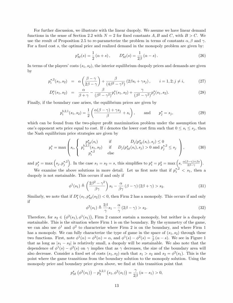
β (α− s). We see in Figure 1that as long as |s1 − s2| is relatively small, a duopoly will be sustainable. We also note that thedependence of φ1(s) − φ2(s) on γ implies that as γ decreases, the size of the boundary area willalso decrease. Consider a fixed set of costs (s1, s2) such that s1 > s2 and s2 = φ2(s1). This is thepoint where the game transitions from the boundary solution to the monopoly solution. Using themonopoly price and boundary price given above, we find at this transition point that

p?M(φ2(s1)

)− pb,2,12

(s1, φ

2(s1))

=γ

2β(α− s1) > 0,

13

6s2

-

s1α

α

���������������������

��

��

��

��

��

��

��

��

��

��

���

���

���

���

���

���

���

����

����

����

����

����

M2B2

Duopoly

B1

M1

φ1(s1)φ2(s1)φ1(s2)

φ2(s2)

Mi = Firm i Monopoly

Bi = Firm j on Boundary

Figure 1: Characterization of solution in cost space

and thus there is a jump in the equilibrium price of Firm 2 as the game transitions from Firm 1 onthe boundary to Firm 2 being a monopoly.

3 Differential Game

The single-period game provides only the beginning of an insight into the pricing decisions offirms. In reality, firms make their decisions dynamically through time. We consider a market inwhich there are N possible firms, each of which has a fixed lifetime capacity of production at timet = 0 denoted by xi(0), and where xi(t) denotes the remaining capacity at time t. The firms inthis market produce only a single good and thus, one can use the terminology firm and productinterchangably. In this sense, xi(t) represents the remaining amount of a certain product that willbe sold. Therefore, when xi = 0, no more of the product will be sold, the firm has exhausted itscapacity and is out of business. Thus, xi is not to be confused with inventory which is typicallyreplenishable. Our point of view abstracts from the microscopic level of inventory fluctuations tothe level of lifetime production. For simplicity of notation, we consider the cost of production inthe dynamic game to be zero, but we will see there are shadow costs associated with scarcity ofgoods as they run down.

Each firm i chooses a Markovian dynamic pricing strategy, pi = pi(x(t)) where x(t) = (x1(t), . . . , xN (t)).This is the price at which consumers can purchase a unit of the good produced by firm i. The firmsin this market produce substitute, but not perfectly substitutable, goods. As in Section 2, giventhese prices, each firm i = 1, . . . , N expects the market to demand at a rate Di(p1, p2, . . . , pN ), butactual demands from the market may see short term unpredictable fluctuations. We model themin the simplest way:

di(t) = Di (p1, p2, . . . , pN )− σiεi(t), (33)

where {εi(t)}i=1,...,N are correlated Gaussian white noise sequences. Consequently, the dynamicsof the lifetime capacity of the firms is given by dxi(t) = −di(t) dt. This leads to the controlled

14

stochastic differential equations

dxi(t) = −Di

(p1(x(t)), . . . , pN (x(t))

)dt+ σi dWi(t), if xi > 0, i = 1, . . . , N, (34)

where {Wi(t)}i=1,...,N are correlated Brownian motions. If xi(t) = 0 for any t, then xi(s) = 0 for alls ≥ t: random shocks cannot resuscitate a firm that has gone out of business. The use of this typeof additive shock in demand is common in the economics literature, for example Arrow et al. [1].The use of a Brownian motion for the demand flow can be found in various sources, for exampleBather [3]. An alternative model for demand uncertainty in the literature is to consider the processof customer arrival as a Poisson process, see for example Besbes and Zeevi [8] for recent work inthis direction.

3.1 The Linear Demand Duopoly Game

Now that we have fully specified the dynamics of the firms’ remaining lifetime capacities, we moveon to the actual study of the dynamic game. The analysis can be done for an arbitrary number ofplayers N , but, to simplify the exposition, we focus on the case N = 2, i.e. duopoly. Additionally,we focus on the case of a linear demand system. This will allow us to be more explicit in our actualresults. See Appendix C for a discussion of the N -player linear demand game.

Given initial lifetime capacity xi(0) > 0, player i = 1, 2 seeks to maximize his expected dis-counted lifetime profit

E{∫ ∞

0e−rtpi(x(t))Di (p1 (x(t)) , p2 (x(t))) 11{xi(t)>0} dt

}, (35)

where r > 0 is a discount rate and Di are the actual demands constructed in Definition 2.2 usingthe linear demand functions given in Section 2.2. We restrict attention to Markov Perfect Nashequilibria in order to rule out equilibria with undesirable properties such as non-credible threats(see, for example, Fudenberg and Tirole [19, Chapter 13]). This means that we are looking for apair (p?1(x(t)), p?2(x(t))) such that for i = 1, 2, j 6= i, and for all x(0) ∈ R2

+,

E{∫ ∞

0e−rtp?i (x(t))Di

(p?i (x(t)) , p?j (x(t))

)11{xi(t)>0} dt

}≥

E{∫ ∞

0e−rtpi(x(t))Di

(pi (x(t)) , p?j (x(t))

)11{xi(t)>0} dt

},

for any Markov strategy pi of player i. (The overbar in p?i is used to distinguish the dynamic Nashequilibrium from the equilibrium of the static game in Section 2).

We define the value functions of the two firms by the coupled optimization problems

Vi(x1, x2) = suppi≥0

E{∫ ∞

0e−rtpi(x(t))Di (p1 (x(t)) , p2 (x(t))) 11{x1(t)>0} dt

}, i = 1, 2. (36)

Then, by a dynamic programming argument for nonzero-sum differential games (see, for example,Friedman [17, Section 8.2], Basar and Olsder [2, Section 6.5.2], or Dockner et al. [13, Section 4.2]),these value functions, if they have sufficient regularity, satisfy the following system of PDEs:

LVi + suppi≥0

{−D1 (p1, p2)

∂Vi∂x1−D2 (p1, p2)

∂Vi∂x2

+ piDi (p1, p2)

}− rVi = 0 (37)

15

for i = 1, 2, where

L =1

2σ21

∂2

∂x21+ ρσ1σ2

∂2

∂x1∂x2+

1

2σ22

∂2

∂x22,

and ρ is the correlation coefficient of the Brownian motions: E {dW1dW2} = ρ dt.When the parameter γ is not too large, both players are close to being monopolists in disjoint

markets for their own goods, and we can expect that the dynamic Nash equilibrium (p?1(x(t)), p?2(x(t)))is such that both demands Di (p?1(x(t)), p?2(x(t))) remain strictly positive while xi(t) > 0. We shallfind that this is indeed the case for small enough γ in the asymptotic solution of Section 3.3 andthe numerical solutions in Section 4.

When both demands are positive, we see easily from Propositions 2.4 and 2.5 that the lineardemand functions satisfy the relationship

Dj(p1, p2) = DM (pj)−γ

βDi(p1, p2), j 6= i, (38)

which allows us to re-write Eqn. (37) as

LVi −DM (pj)∂Vi∂xj

+ suppi≥0

{Di (p1, p2) ·

[pi −

(∂Vi∂xi− γ

β

∂Vi∂xj

)]}− rVi = 0, i = 1, 2. (39)

We now observe that the Nash equilibrium problem in the two PDEs in Eqn. (39) is exactly a staticNash equilibrium problem for a two-player Bertand game, but with costs

Si (x) ,∂Vi∂xi

(x)− γ

β

∂Vi∂xj

(x) , i = 1, 2. (40)

Given the unique Nash equilibrium p?i (S1 (x) , S2 (x)) of this static problem from Proposition2.6, the PDE system is simply

LVi −DM

(p?j (S1 (x) , S2 (x))

) ∂Vi∂xj

+Gi (S1 (x) , S2 (x))− rVi = 0, i, j = 1, 2; j 6= i, (41)

where we define Gi(s1, s2) = Di (p?1, p?2) (p?i − si) as the equilibrium profit function of the static

game.The domain of the PDE problem is x1 > 0, x2 > 0. When one firm runs out of capacity, the

other has a monopoly. We denote by vM (x) the value function of a monopolist with remainingcapacity x, which we will study in the next section. On x2 = 0, x1 > 0, Firm 1 has a monopoly, soV2(x1, 0) ≡ 0 and V1(x1, 0) = vM (x1). On x1 = 0, x2 > 0, Firm 2 has a monopoly, so V1(0, x2) ≡ 0and V2(0, x2) = vM (x2).

As is well known, it is extremely difficult to provide existence and regularity results for systemsof PDEs arising from nonzero-sum differential games and we do not attempt to do so here. Someresults on weak solutions are found in Bensoussan and Frehse [4, 5], for related problems on smoothbounded domains with absorbing boundary conditions. In contrast, zero-sum games, which arecharacterized by a scalar equation, have a well studied viscosity theory; see, for example Flemingand Souganidis [16]. Mean Field Games are an intermediate case characterized by a system of twoPDEs and some regularity results exist (Lasry and Lions [25]). We also mention some analyticalprogress can be made in nonzero-sum stochastic differential games of Dynkin type, that is gameson stopping times; see Hamadene and Zhang [21].

In the stochastic game, the intuition is that the elliptic operator L will provide regularitywhich is supported in the numerical results of Section 4. In the non-stochastic game, when γ issmall enough, we obtain regular asymptotic approximations in Section 3.3 because the strength ofcompetition between firms is weak.

16

3.2 Monopoly Problem

When one firm has a monopoly over the market, the dynamics for the firm’s remaining capacity,x(t), is given by

dx(t) = −DM (p(x(t))) dt+ σdW (t),

where W is a Brownian motion. The value function of the monopoly firm as a function of its initialcapacity x0 = x ∈ R+ is defined to be the maximum expected discounted lifetime profit

vM (x) , supp≥0

E{∫ ∞

0e−rtp (x(t))DM (p (x(t))) 11{x(t)>0} dt

}. (42)

The associated Bellman equation for this stochastic control problem is the ODE

1

2σ2v′′M + sup

p≥0

{DM (p)

(p− v′M

)}− rvM = 0,

with boundary condition vM (0) = 0. We look for solutions in which limx→∞ v′M (x) = 0.

As we are working in the case of linear demands, we find from Eqn. (26):

1

2σ2v′′M +

1

4β

(v′M − α

)2 − rvM = 0. (43)

In the case σ = 0, the monopoly ODE is given by

1

4β

(v′M − α

)2 − rvM = 0, (44)

and we can find an explicit solution.

Proposition 3.1. The value function for the monopoly with σ = 0 is

vM (x) =α2

4βr

[W(−e−µx−1

)+ 1]2, (45)

where µ = (2βr)/α and W is the Lambert W function defined by the relation Y = W(Y )eW(Y )

with domain Y ≥ −e−1.

Proof. It is straightforward to check that the Lambert W function satisfies W(z) < 0 for z ∈[−e−1, 0), W

(−e−1

)= −1, W(0) = 0, and W′(z) = W(z)/ (z (1 + W(z))) for z > −e−1, and

therefore that Eqn. (45) indeed satisfies Eqn. (44) and the boundary condition vM (0) = 0. Wenote that the restriction of the domain of W to [−e−1,∞) is sufficient as the argument to W inEqn. (45) is equal to −e−1 when x = 0 and increases to zero as x increases to infinity. �

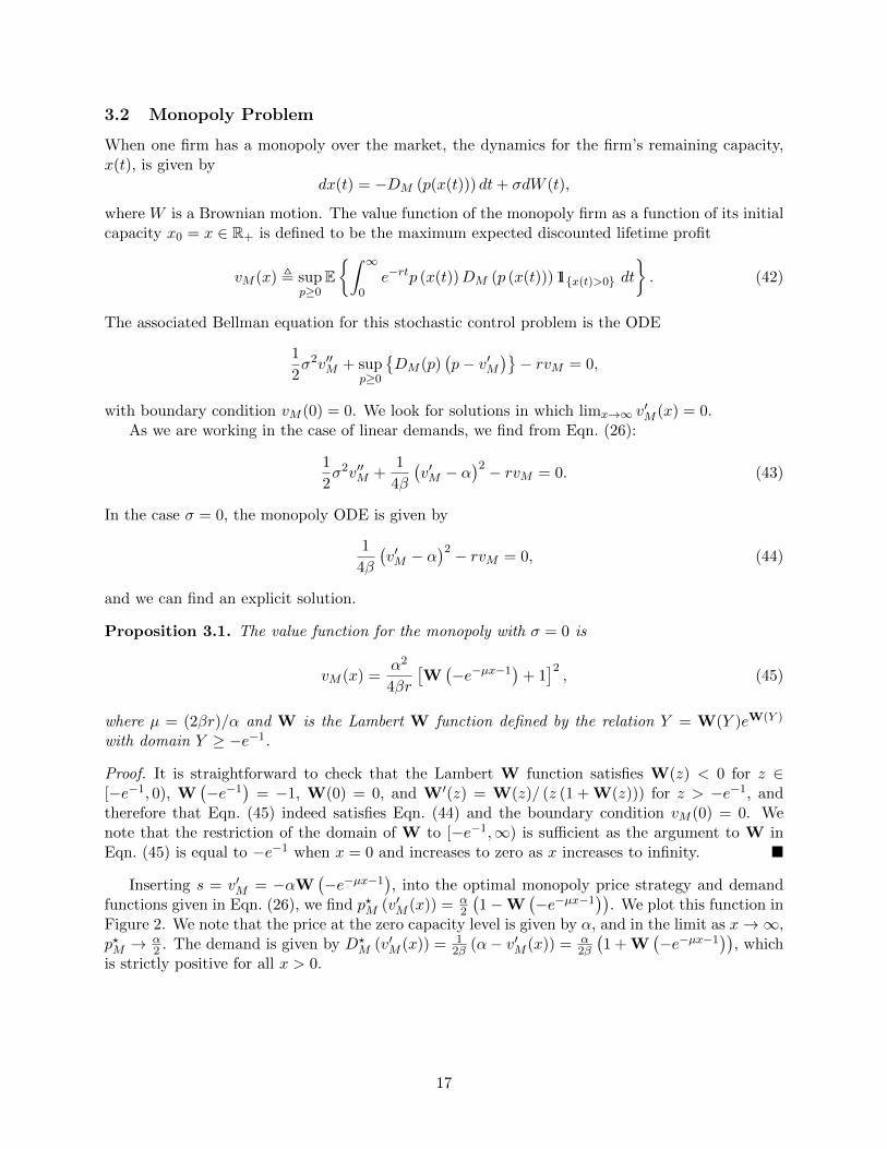
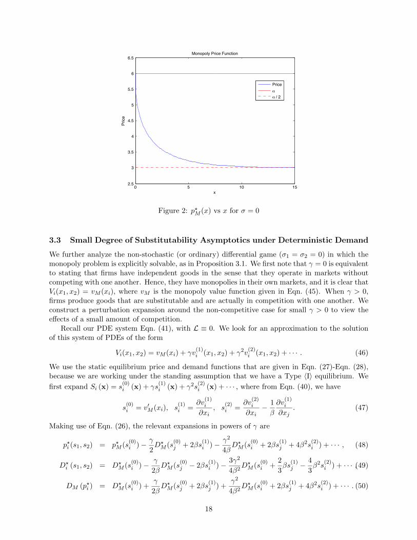
Inserting s = v′M = −αW(−e−µx−1

), into the optimal monopoly price strategy and demand

functions given in Eqn. (26), we find p?M (v′M (x)) = α2

(1−W

(−e−µx−1

)). We plot this function in

Figure 2. We note that the price at the zero capacity level is given by α, and in the limit as x→∞,p?M →

α2 . The demand is given by D?

M (v′M (x)) = 12β (α− v′M (x)) = α

2β

(1 + W

(−e−µx−1

)), which

is strictly positive for all x > 0.

17

0 5 10 152.5

3

3.5

4

4.5

5

5.5

6

6.5Monopoly Price Function

x

Price

Priceα

α / 2

Figure 2: p?M (x) vs x for σ = 0

3.3 Small Degree of Substitutability Asymptotics under Deterministic Demand

We further analyze the non-stochastic (or ordinary) differential game (σ1 = σ2 = 0) in which themonopoly problem is explicitly solvable, as in Proposition 3.1. We first note that γ = 0 is equivalentto stating that firms have independent goods in the sense that they operate in markets withoutcompeting with one another. Hence, they have monopolies in their own markets, and it is clear thatVi(x1, x2) = vM (xi), where vM is the monopoly value function given in Eqn. (45). When γ > 0,firms produce goods that are substitutable and are actually in competition with one another. Weconstruct a perturbation expansion around the non-competitive case for small γ > 0 to view theeffects of a small amount of competition.

Recall our PDE system Eqn. (41), with L ≡ 0. We look for an approximation to the solutionof this system of PDEs of the form

Vi(x1, x2) = vM (xi) + γv(1)i (x1, x2) + γ2v

(2)i (x1, x2) + · · · . (46)

We use the static equilibrium price and demand functions that are given in Eqn. (27)-Eqn. (28),because we are working under the standing assumption that we have a Type 〈I〉 equilibrium. We

first expand Si (x) = s(0)i (x) + γs

(1)i (x) + γ2s

(2)i (x) + · · · , where from Eqn. (40), we have

s(0)i = v′M (xi), s

(1)i =

∂v(1)i

∂xi, s

(2)i =

∂v(2)i

∂xi− 1

β

∂v(1)i

∂xj. (47)

Making use of Eqn. (26), the relevant expansions in powers of γ are

p?i (s1, s2) = p?M (s(0)i )− γ

2D?M (s

(0)j + 2βs

(1)i )− γ2

4βD?M (s

(0)i + 2βs

(1)j + 4β2s

(2)i ) + · · · , (48)

D?i (s1, s2) = D?

M (s(0)i )− γ

2βD?M (s

(0)j − 2βs

(1)i )− 3γ2

4β2D?M (s

(0)i +

2

3βs

(1)j −

4

3β2s

(2)i ) + · · · ,(49)

DM (p?i ) = D?M (s

(0)i ) +

γ

2βD?M (s

(0)j + 2βs

(1)j ) +

γ2

4β2D?M (s

(0)i + 2βs

(1)j + 4β2s

(2)i ) + · · · . (50)

18

We define

q(x) , D?M

(v′M (x)

)=

1

2β

(α− v′M (x)

). (51)

Then, inserting Eqn. (46) into Eqn. (41), using Eqn. (48)-Eqn. (50), and comparing terms in γ and

γ2, give that v(1)i and v

(2)i satisfy

q(x1)∂v

(1)i

∂x1+ q(x2)

∂v(1)i

∂x2+ rv

(1)i = −q(x1)q(x2), (52)

q(x1)∂v

(2)i

∂x1+ q(x2)

∂v(2)i

∂x2+ rv

(2)i =

1

2β

(∂v

(1)j

∂xj+ q(xi)

)·

(∂v

(1)i

∂xj+ q(xi)

)

+1

4β

(∂v

(1)i

∂xi+ q(xj)

)2

− 3

2β(q(xi))

2 , (53)

for i = 1, 2 and j 6= i, with boundary conditions v(1)1 (x1, 0) = v

(2)1 (x1, 0) = 0 and v

(1)1 (0, x2) =

v(2)1 (0, x2) = 0.

Proposition 3.2. The solution v(1)i is given, for x1 > x2, by

v(1)1 (x1, x2) =

α2

4β2r

(e−rQ(x2) (1 + rQ(x2))− e−rQ(x1) (1− rQ(x2)) + e−r(Q(x1)+Q(x2)) − 1

), (54)

where

Q(x) ,∫ x

0

1

q(u)du = −1

rlog(−W

(−e−µx−1

)), (55)

and, for x2 ≥ x1, by reversing the roles of x1 and x2 in Eqn. (54). The solution for v(1)2 is clearly

the same, i.e. v(1)2 ≡ v(1)1 .

Proof. The first step is to make the change of variables (ξ, η) = (Q(x1), Q(x2)) and u(ξ, η) =

er2(ξ+η)v

(1)i

(Q−1(ξ), Q−1(η)

)in Eqn. (52), which gives

∂u

∂ξ+∂u

∂η= f(ξ, η), ξ, η > 0; u(ξ, 0) = u(0, η) = 0, (56)

where f(ξ, η) , −er2(ξ+η)q

(Q−1(ξ)

)q(Q−1(η)

). We see by the symmetry of this equation that

u(ξ, η) = u(η, ξ). We first suppose that ξ > η and solve the PDE with the boundary conditionu(ξ, 0) = 0. The other half of the solution can be obtained by symmetry. The solution is

u(ξ, η) =

∫ η

0f(s+ ξ − η, s) ds = −

∫ η

0e

r2(ξ−η+2s)q

(Q−1 (s+ ξ − η)

)q(Q−1 (s)

)ds. (57)

By the definition of q(x) in Eqn. (51) and vM in Eqn. (45), we have q(x) = α2β

[1 + W

(−e−µx−1

)].

This leads to Eqn. (55) since the range of W(−e−µx−1

)is (−1, 0). From properties of the Lambert

W function, it follows easily that −e−rs = W(−e−µQ−1(s)−1

), and hence

q(Q−1(s)

)=

α

2β

(1 + W

(−e−µQ−1(s)−1

))=

α

2β

(1− e−rs

). (58)

We can now easily compute the integral in Eqn. (57). After restoring the transformations, weobtain Eqn. (54). �

19

Remark 3.1. It can be verified by direct computation that the solutions v(1)i in Proposition 3.2

are C1 on the line x1 = x2. One can also solve the PDEs in Eqn. (53) to obtain a second-ordercorrection for the value functions. We present this solution in Appendix B.

Remark 3.2. While we do not give a formal convergence proof for the asymptotic approximation,

we note that, since v(1)i and v

(2)i are bounded with bounded continuous first-derivatives, the error

terms Ei defined by Vi = vM + γv(1)i + γ2v

(2)i + Ei solve

q(x1)∂Ei∂x1

+ q(x2)∂Ei∂x2

+ rEi = O(γ3)

with Ei(x1, 0) = Ei(0, x2) = 0. It follows from here that, for fixed x1, x2 > 0, |Ei(x1, x2)| = O(γ3)as γ ↓ 0.

3.4 Discussion of Asymptotic Solution

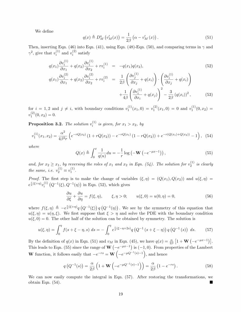
We plot v(1)1 in Figure 3(a). Intuitively, it decreases from zero on the axes, because the first order

correction decreases the value of the game due to the transition from a one-player monopoly to atwo-player duopoly game. Hence, the greater the value of γ, the lower is the lifetime profit of anindividual firm.

0

5

10

15

20

05

1015

20

−10

−8

−6

−4

−2

0

x2

v1(1)

x1

(a) v(1)1 : Surface

05

1015

20

05

1015

20

−2.5

−2

−1.5

−1

−0.5

0

x1

v1(2)

x2

(b) v(2)1 : Surface

Figure 3: v(1)1 and v

(2)1 . First- and second-order value function corrections.

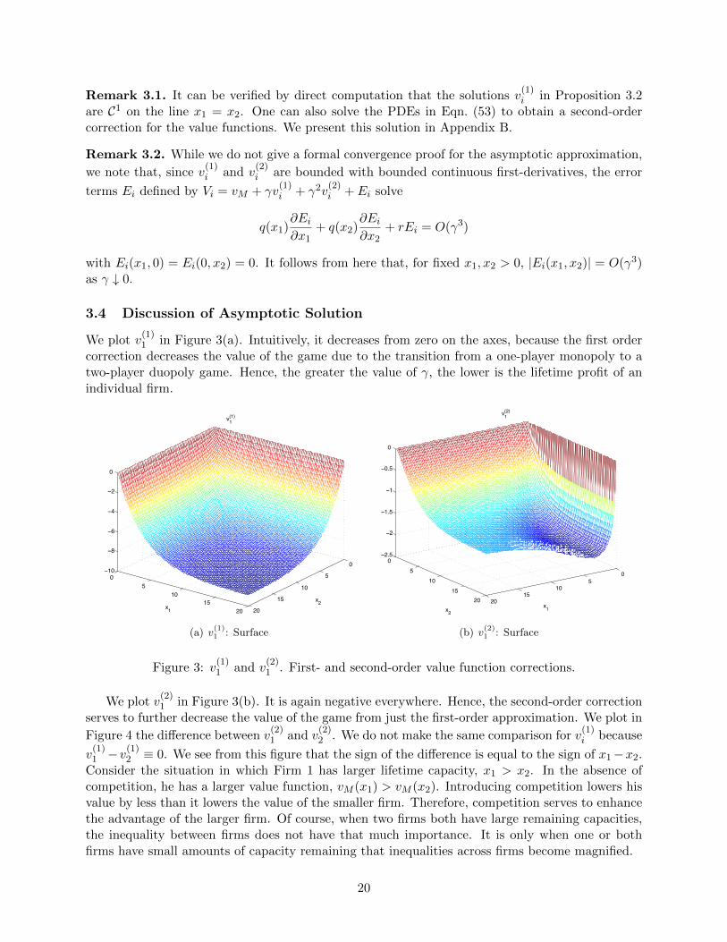
We plot v(2)1 in Figure 3(b). It is again negative everywhere. Hence, the second-order correction

serves to further decrease the value of the game from just the first-order approximation. We plot in

Figure 4 the difference between v(2)1 and v

(2)2 . We do not make the same comparison for v

(1)i because

v(1)1 −v

(1)2 ≡ 0. We see from this figure that the sign of the difference is equal to the sign of x1−x2.

Consider the situation in which Firm 1 has larger lifetime capacity, x1 > x2. In the absence ofcompetition, he has a larger value function, vM (x1) > vM (x2). Introducing competition lowers hisvalue by less than it lowers the value of the smaller firm. Therefore, competition serves to enhancethe advantage of the larger firm. Of course, when two firms both have large remaining capacities,the inequality between firms does not have that much importance. It is only when one or bothfirms have small amounts of capacity remaining that inequalities across firms become magnified.

20

05

1015

20

05

1015

20

−2

−1.5

−1

−0.5

0

0.5

1

1.5

2

x1

v1(2) − v2

(2)

x2

Figure 4: v(2)1 −v

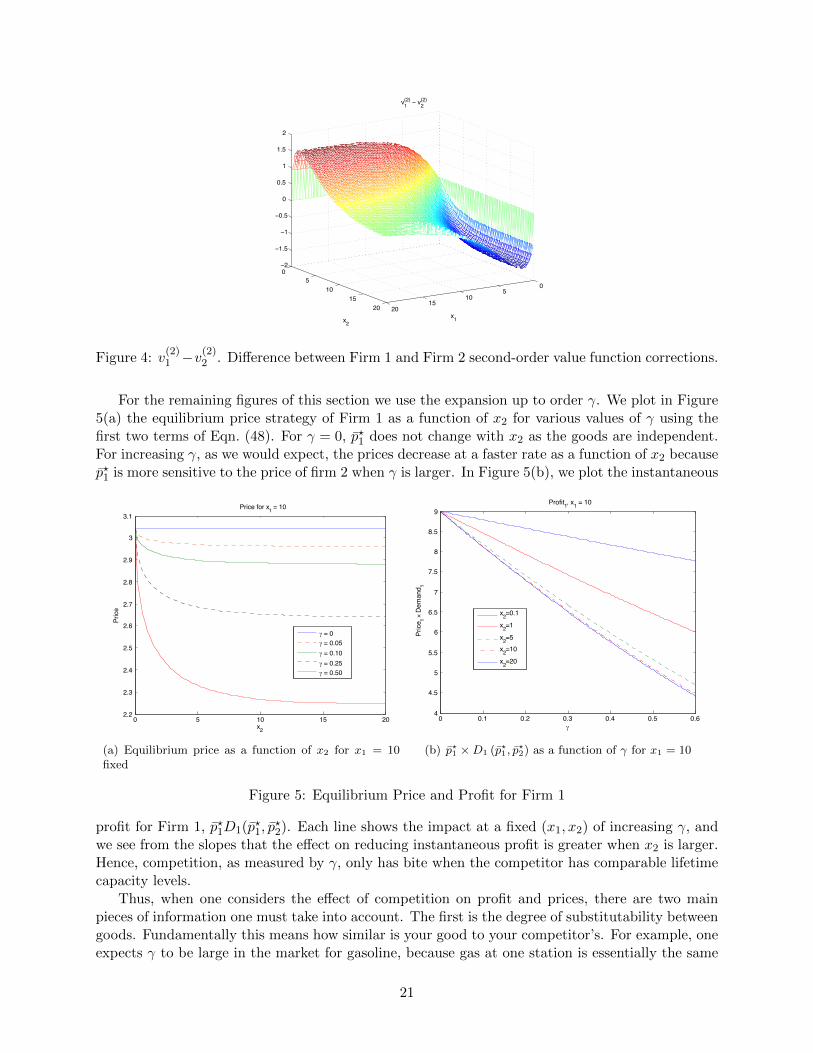
(2)2 . Difference between Firm 1 and Firm 2 second-order value function corrections.

For the remaining figures of this section we use the expansion up to order γ. We plot in Figure5(a) the equilibrium price strategy of Firm 1 as a function of x2 for various values of γ using thefirst two terms of Eqn. (48). For γ = 0, p?1 does not change with x2 as the goods are independent.For increasing γ, as we would expect, the prices decrease at a faster rate as a function of x2 becausep?1 is more sensitive to the price of firm 2 when γ is larger. In Figure 5(b), we plot the instantaneous

0 5 10 15 202.2

2.3

2.4

2.5

2.6

2.7

2.8

2.9

3

3.1Price for x1 = 10

x2

Price

γ = 0γ = 0.05γ = 0.10γ = 0.25γ = 0.50

(a) Equilibrium price as a function of x2 for x1 = 10fixed

0 0.1 0.2 0.3 0.4 0.5 0.64

4.5

5

5.5

6

6.5

7

7.5

8

8.5

9Profit1, x1 = 10

γ

Price

1 × De

man

d 1

x2=0.1

x2=1

x2=5x2=10

x2=20

(b) p?1 ×D1 (p?1, p?2) as a function of γ for x1 = 10

Figure 5: Equilibrium Price and Profit for Firm 1

profit for Firm 1, p?1D1(p?1, p

?2). Each line shows the impact at a fixed (x1, x2) of increasing γ, and

we see from the slopes that the effect on reducing instantaneous profit is greater when x2 is larger.Hence, competition, as measured by γ, only has bite when the competitor has comparable lifetimecapacity levels.

Thus, when one considers the effect of competition on profit and prices, there are two mainpieces of information one must take into account. The first is the degree of substitutability betweengoods. Fundamentally this means how similar is your good to your competitor’s. For example, oneexpects γ to be large in the market for gasoline, because gas at one station is essentially the same

21

as gas at a station across the street. The goods are not perfect substitutes because of travel costs,brand loyalty, and a host of other reasons. However, in the market for CDs, one expects a verylow degree of substitutability, because an individual artist’s music is typically highly differentiatedfrom that of another artist, even within a specific genre. It is reasonable to assume in such a marketthat γ is quite low.

The second main piece of information is how credible is your competition. In this model, theproxy for a credible competitor is their level of lifetime capacity. If your competitor has very littlelifetime capacity, then it stands to reason that regardless of how similar their good is to your owngood, you will be a monopoly in short order. In contrast, if your competitor has a large amountof lifetime capacity, then they are a very credible threat to your business. As such, you must takesuch them very seriously even if their good is highly differentiated (but still substitutable) withyour good. This can be seen in Figure 5(b) as even with γ = 0.1, when x2 is large relative to x1,the instantaneous profit is much less than when x2 is relatively small.

In Figure 6, we plot the solution to dx1dt = −D1 (p?1(x), p?2(x)), where we have used our expansion

of order γ. We present the path of x1(t) over time for various different values of γ starting fromx1(0) = x2(0) = 10. We see that as γ increases, the time of the game increases. That is, ittakes more time for Firm 1 to deplete their lifetime capacity when the degree of substitutability isgreater. We can see this also by looking at the path of both demand and prices over the time of

0 2 4 6 8 100

1

2

3

4

5

6

7

8

9

10Path of game for Firm 1

Time

x 1(t)

γ=0.05γ=0.1γ=0.2γ=0.4γ=0.6

Figure 6: Path of Firm 1 Lifetime Capacity over time with x1(0) = x2(0) = 10 for various valuesof γ

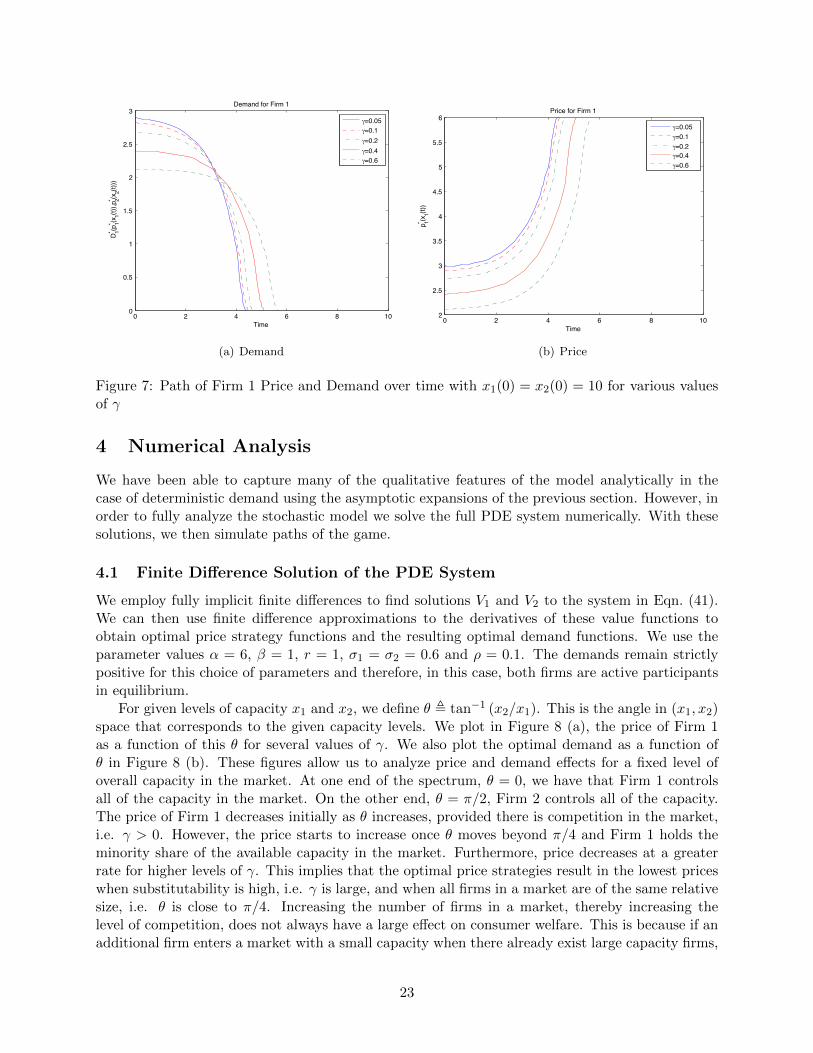
the game. These are plotted in Figures 7 (a) and (b), respectively. We see that, for an individualfirm, increasing the value of γ drives down the price, while the demand first decreases and thenincreases. Common across all levels of γ, we see that as the capacity of the firm diminishes overtime, the price increases while demand decreases.

Finally, we remark that one can confirm that the resulting demands from the asymptotic ap-proximation for both firms are strictly positive in equilibrium. Therefore, our previous assumptionon strictly positive demands is justified at least for γ small enough.

22

0 2 4 6 8 100

0.5

1

1.5

2

2.5

3Demand for Firm 1

Time

D 1* (p1* (x

1(t)),p

2* (x2(t)

))

γ=0.05γ=0.1γ=0.2γ=0.4γ=0.6

(a) Demand

0 2 4 6 8 102

2.5

3

3.5

4

4.5

5

5.5

6Price for Firm 1

Time

p 1* (x1(t)

)

γ=0.05γ=0.1γ=0.2γ=0.4γ=0.6

(b) Price

Figure 7: Path of Firm 1 Price and Demand over time with x1(0) = x2(0) = 10 for various valuesof γ

4 Numerical Analysis

We have been able to capture many of the qualitative features of the model analytically in thecase of deterministic demand using the asymptotic expansions of the previous section. However, inorder to fully analyze the stochastic model we solve the full PDE system numerically. With thesesolutions, we then simulate paths of the game.

4.1 Finite Difference Solution of the PDE System

We employ fully implicit finite differences to find solutions V1 and V2 to the system in Eqn. (41).We can then use finite difference approximations to the derivatives of these value functions toobtain optimal price strategy functions and the resulting optimal demand functions. We use theparameter values α = 6, β = 1, r = 1, σ1 = σ2 = 0.6 and ρ = 0.1. The demands remain strictlypositive for this choice of parameters and therefore, in this case, both firms are active participantsin equilibrium.

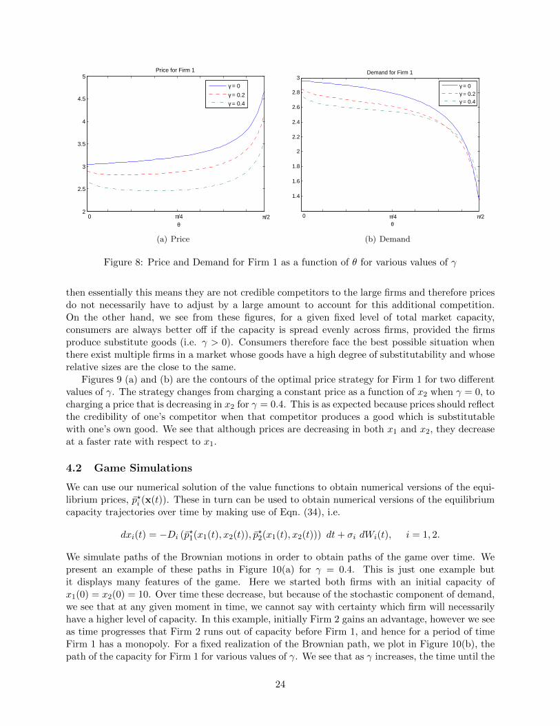
For given levels of capacity x1 and x2, we define θ , tan−1 (x2/x1). This is the angle in (x1, x2)space that corresponds to the given capacity levels. We plot in Figure 8 (a), the price of Firm 1as a function of this θ for several values of γ. We also plot the optimal demand as a function ofθ in Figure 8 (b). These figures allow us to analyze price and demand effects for a fixed level ofoverall capacity in the market. At one end of the spectrum, θ = 0, we have that Firm 1 controlsall of the capacity in the market. On the other end, θ = π/2, Firm 2 controls all of the capacity.The price of Firm 1 decreases initially as θ increases, provided there is competition in the market,i.e. γ > 0. However, the price starts to increase once θ moves beyond π/4 and Firm 1 holds theminority share of the available capacity in the market. Furthermore, price decreases at a greaterrate for higher levels of γ. This implies that the optimal price strategies result in the lowest priceswhen substitutability is high, i.e. γ is large, and when all firms in a market are of the same relativesize, i.e. θ is close to π/4. Increasing the number of firms in a market, thereby increasing thelevel of competition, does not always have a large effect on consumer welfare. This is because if anadditional firm enters a market with a small capacity when there already exist large capacity firms,

23

2

2.5

3

3.5

4

4.5

5Price for Firm 1

θ

γ = 0

γ = 0.2

γ = 0.4

0 π/2π/4

(a) Price

1.4

1.6

1.8

2

2.2

2.4

2.6

2.8

3Demand for Firm 1

θ

γ = 0γ = 0.2γ = 0.4

0 π/2π/4

(b) Demand

Figure 8: Price and Demand for Firm 1 as a function of θ for various values of γ

then essentially this means they are not credible competitors to the large firms and therefore pricesdo not necessarily have to adjust by a large amount to account for this additional competition.On the other hand, we see from these figures, for a given fixed level of total market capacity,consumers are always better off if the capacity is spread evenly across firms, provided the firmsproduce substitute goods (i.e. γ > 0). Consumers therefore face the best possible situation whenthere exist multiple firms in a market whose goods have a high degree of substitutability and whoserelative sizes are the close to the same.

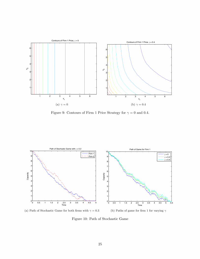
Figures 9 (a) and (b) are the contours of the optimal price strategy for Firm 1 for two differentvalues of γ. The strategy changes from charging a constant price as a function of x2 when γ = 0, tocharging a price that is decreasing in x2 for γ = 0.4. This is as expected because prices should reflectthe credibility of one’s competitor when that competitor produces a good which is substitutablewith one’s own good. We see that although prices are decreasing in both x1 and x2, they decreaseat a faster rate with respect to x1.

4.2 Game Simulations

We can use our numerical solution of the value functions to obtain numerical versions of the equi-librium prices, p?i (x(t)). These in turn can be used to obtain numerical versions of the equilibriumcapacity trajectories over time by making use of Eqn. (34), i.e.

dxi(t) = −Di (p?1(x1(t), x2(t)), p?2(x1(t), x2(t))) dt+ σi dWi(t), i = 1, 2.

We simulate paths of the Brownian motions in order to obtain paths of the game over time. Wepresent an example of these paths in Figure 10(a) for γ = 0.4. This is just one example butit displays many features of the game. Here we started both firms with an initial capacity ofx1(0) = x2(0) = 10. Over time these decrease, but because of the stochastic component of demand,we see that at any given moment in time, we cannot say with certainty which firm will necessarilyhave a higher level of capacity. In this example, initially Firm 2 gains an advantage, however we seeas time progresses that Firm 2 runs out of capacity before Firm 1, and hence for a period of timeFirm 1 has a monopoly. For a fixed realization of the Brownian path, we plot in Figure 10(b), thepath of the capacity for Firm 1 for various values of γ. We see that as γ increases, the time until the

24

x1

x 2

Contours of Firm 1 Price, γ = 0

1 2 3 4 5 6

1

2

3

4

5

6

(a) γ = 0

x1

x 2

Contours of Firm 1 Price, γ = 0.4

1 2 3 4 5 6

1

2

3

4

5

6

(b) γ = 0.4

Figure 9: Contours of Firm 1 Price Strategy for γ = 0 and 0.4.

0 0.5 1 1.5 2 2.5 3 3.5 4 4.5 50

1

2

3

4

5

6

7

8

9

10Path of Stochastic Game with γ = 0.2

Time

Capa

city

Firm 1Firm 2

(a) Path of Stochastic Game for both firms with γ = 0.3

0 0.5 1 1.5 2 2.5 3 3.5 4 4.5 5 5.50

1

2

3

4

5

6

7

8

9

10Path of Game for Firm 1

Time

Capa

city

γ = 0γ = 0.2γ = 0.4

(b) Paths of game for firm 1 for varying γ

Figure 10: Path of Stochastic Game

25

capacity of Firm 1 is exhausted, also appears to increase. This effect, where increased competitionprolongs the lifetime of firms, is consistent with what we saw in Figure 6 in the deterministic game.

5 Conclusion

We have studied nonzero-sum stochastic differential games arising from Bertrand competitions, inparticular, the case of a duopoly with linear demand functions. By considering the case wherethere is a small degree of substitutability between the firms’ goods, we are able to construct anasymptotic approximation that captures many of the qualitative features of the ordinary differentialgame. Numerical solutions further provide insight into the stochastic case and where there is ahigher degree of substitutability. In our study of the dynamic game, we concentrated on the casewhere both firms have positive demand in equilibrium. As we saw in the static game, it is possiblefor there to arise cases where this does not occur. However, the study of such cases remains aninteresting open question in the analysis of these dynamic Bertrand games.

These tools allow us to quantify the effects of substitutability and relative firm size on prices,demands and profits. In particular, we find that consumers benefit the most when a market isstructured with many firms of the same relative size producing highly substitutable goods. However,a large degree of substitutability does not always lead to large drops in price, for example whentwo firms have a large difference in their size. That is, consumers benefit the most when firms arecompeting with other firms whom they deem to be credible threats. A competitor is a crediblethreat only if they have capacity large enough to match their competitors. For example, theexistence of a very small coffee shop does not greatly affect the pricing decisions of Starbucks.

It is of interest to extend the analysis here to markets with nonlinear demand systems as well asto random demand environments. By the latter, we mean that baseline demand and substitutabilitymay vary stochastically over time with economic conditions or consumer tastes. For example, inthe linear demand system Eqn. (2), there may be fluctuations in the intercept parameter A, whichis a measure of the general level of demand due to business cycles and recessions, or in C/B, whichis the measure of substitutability, as certain brands fall out of fashion, for example what Toyotais experiencing in 2010. Finally, an important related direction is to connect, in a probabilisticway, prices to the mechanism of customer arrival, for example, by making the arrival intensity afunction of prices. Such models have been used in a variety of applications for the single-playerprice setting problem. However, their use in competitive markets leads to multi-player stochasticdifferential games with jumps, and is a direction we are currently pursuing.

A Proof of Proposition 2.2

We have assumed that pN exists. We show that this implies pN−1 exists. The result for all n willthen follow by induction. Fix p1, . . . , pN−2 and denote this vector of prices by ρ. Let pN−1 be anarbitrary price. We denote pN (ρ, pN−1) by p. We then have two cases, depending on pN−1, underwhich we wish to show DN−1

N−1 (ρ, pN−1) < 0. The first case is pN−1 > pN (ρ, p), which implies

DN−1N−1 (ρ, pN−1) = DN

N−1 (ρ, pN−1, p) = DNN (ρ, p, pN−1) < DN

N (ρ, p, p (ρ, p)) = 0.

The second case we must consider is the reverse inequality, i.e. pN−1 < pN (ρ, p). This implies

0 = DNN (ρ, pN−1, p) > DN

N (ρ, p (ρ, p) , p) = DNN−1 (ρ, p, p (ρ, p)) = DN−1

N−1 (ρ, p) .

26

Hence, regardless of the relative size of pN−1 and pN (ρ, p), we have that DN−1N−1(p) is negative for

some vector of prices p. We have ignored the case pN−1 = pN (ρ, p), because this would change theabove inequalities to equalities and we would have the choke price we are looking for.

We know by Assumption 2.4 that DN−1N−1 is a decreasing function of pN−1. We have shown above

that there exists some vector of prices p such that DN−1N−1(p) < 0. We thus need only show that

there exists some vector of prices p where DN−1N−1(p) > 0. This will establish the existence of the

choke price.Fix some vector of prices p = (p1, . . . , pN−2, 0), where p1, . . . , pN−2 are arbitrary prices. Denote

by 0 the vector in RN−1 of all zeros. Recall that DNN (0, 0) > DN

N (0, pN (0)) = 0. This impliespN (0) > 0. We then have

DN−1N−1 (p) = DN

N−1 (p, pN (p)) ≥ DNN−1 (p, pN (0)) > DN

N−1 (p, 0) ≥ DNN−1 (0, 0) = DN

N (0, 0) > 0.

Hence, for the vector p we have that DN−1N−1(p) is positive. Therefore, there must exist some pN−1

for every set of prices p1, . . . , pN−2 such that DN−1N−1 (p1, . . . , pN−2, pN−1) = 0.

B Second-order approximation

We give the solution of the PDEs Eqn. (53) for v(2)i . Using the solution to v

(1)i found in Proposition

3.2, making the same change of variables (ξ, η) = (Q(x1), Q(x2)) and solving leads to

v(2)1 =

α2

8β3e−rQ(x2)

[−Q(x2)

2

2

(2rerQ(x2)

erQ(x2) − 1+

rϕ1

1− e−rQ(x1)

)− Q(x2)(1− ϕ1)

1− e−rQ(x1)

+3

2r

(erQ(x2) − 1

)− (1− ϕ1)

2

2r(erQ(x2)

(1− e−rQ(x1)

)) +1− ϕ1

2r

−3

r

(erQ(x2) − ϕ2

1e−rQ(x2) − 1 + ϕ2

1 − 2ϕ1rQ(x2))]. (59)

for x1 > x2 where ϕ1 = exp {−r (Q(x1)−Q(x2))}. For x2 > x1,

v(2)1 =

α2

8β3e−rQ(x1)

[−Q(x1)

2

2

(rerQ(x1)

erQ(x1) − 1+

2rϕ2

1− e−rQ(x2)

)− 2Q(x1)(1− ϕ2)

1− e−rQ(x2)

+3

2r

(erQ(x1) − 1

)− (1− ϕ2)

2

rerQ(x1)(1− e−rQ(x2)

) +1− ϕ2

r

−3

r

(erQ(x1) − 2rQ(x1)− e−rQ(x1)

)]. (60)

where ϕ2 = exp {−r (Q(x2)−Q(x1))}. We omit the details of this lengthy calculation.

C N-player Stochastic Differential Game with Linear Demands

Consider the N -player dynamic Bertrand game under the linear demand system introduced inSection 3. Within this section we explicitly assume that all firms participate in equilibrium, i.e.all firms receive positive demand. In the language of Section 2, this would mean that the resulting

27

dynamic equilibrium is of Type 〈I〉. Let Vi(x) denote the value functions defined by the N -playeranalog of Eqn. (36). Then, the associated PDE system, analog of Eqn. (37), is

LVi + suppi≥0

{−

N∑k=1

DNk (p)

∂Vi∂xk

+ piDNi (p)

}− rVi = 0, i = 1, . . . , N, (61)

where we explicitly denote the dependence of the demand functions on N to indicate the size ofthe vector p in the argument. Here,

L =1

2

N∑i=1

N∑j=1

Σij∂2Vi∂xi∂xj

, (62)

where (Σij)i,j=1,...,N is the covariance matrix between the Brownian motions in Eqn. (34).For a fixed i, we note that we can write

DNj (p) = −C

BDNi (p) +A

(1 +

C

B

)−B

(1− C2

B2

)pj + C

(1 +

C

B

)∑k 6=jk 6=i

pk

= −CBDNi (p) +DN−1

πi(j)(p−i) , (63)

where p−i = p\{pi} and

πi(k) =

{k, k < i

k − 1, k > i.(64)

This decomposition means that one can represent a firm’s demand function at the level N as a linearcombination of another given firm’s demand function at the level N and their own demand functionat the level N − 1 with the given firm being removed. This is a consequence of the consistency ofdemand functions and the existence of choke prices.

Hence, using this decomposition, we have, for i = 1, . . . , N

LVi −N∑k 6=i

DN−1πi(k)

(p−i)∂Vi∂xk

+ suppi≥0

DNi (p)

pi − ∂Vi∂xi

+C

B

∑k 6=i

∂Vi∂xk

− rVi = 0. (65)

Therefore, we can use the results of the static Bertrand game to write the PDEs as

LVi −N∑k 6=i

DN−1πi(k)

(p?−i)∂Vi∂xk

+GNi (s1, . . . , sN ) = rVi (66)

where the prices p? are the solutions of the N -player static game with costs

Si(x) =∂Vi∂xi− C

B

∑k 6=i

∂Vi∂xk

, i = 1, . . . , N (67)

and with corresponding profit functions GNi (s1, . . . , sN ) = DNi (p?) (p?i − si).

The boundary conditions for this PDE depends on the PDEs that result by considering a marketwith N − 1 firms. That is, on any edge of an orthant where xi = 0 and xj > 0 for all j 6= i, wehave Vi ≡ 0 and that Vj solve the same PDE problem except where firm i is removed and thusthere are N − 1 firms in the market. This is similar to the duopoly problem where the boundarycondition depends on the monopoly problem. The remaining conditions can be worked out in asimilar fashion.

28

References

[1] K. J. Arrow, T. Harris, and J. Marschak. Optimal Inventory Policy. Econometrica, 19(3):250–272,1951.

[2] T. Basar and G. J. Olsder. Dynamic Noncooperative Game Theory. Academic Press, 2nd edition, 1995.

[3] J. A. Bather. A Continuous Time Inventory Model. Journal of Applied Probability, 3(2):538–549, 1966.

[4] A. Bensoussan and J. Frehse. Nonlinear elliptic systems in stochastic game theory. Journal fur dieReine und Angewandte Mathematik, 8(Band 350):24–67, 1984.

[5] A. Bensoussan and J. Frehse. Regularity results for nonlinear elliptic systems and applications. Springer,2002.

[6] A. Bensoussan, D. Diltz, and C. Ho. Real options in Stackelberg games with an arithmetic Brownianmotion cash flow process. Preprint, University of Texas at Dallas, 2009.

[7] J. Bertrand. Theorie mathematique de la richesse sociale. Journal des Savants, 67:499–508, 1883.

[8] O. Besbes and A. Zeevi. Dynamic Pricing Without Knowing the Demand Function: Risk Bounds andNear-Optimal Algorithms. Operations Research, 57(6):1407–1420, 2009.

[9] T. Bjork and A. Murgoci. A General Theory of Markovian Time Inconsistent Stochastic ControlProblems. Preprint. Stockholm School of Economics, September 2008.

[10] E. Chamberlin. The Theory of Monopolistic Competition. Harvard University Press, Cambridge, MA,1933.

[11] A. Cournot. Recherches sur les Principes Mathematique de la Theorie des Richesses. Hachette, Paris,1838. English translation by N.T. Bacon, published in Economic Classics, Macmillan, 1897, andreprinted in 1960 by Augustus M. Kelley.

[12] C. d’Aspremont, J. Gamszewicz, and J.-F. Thisse. On Hotelling’s “Stability in Competition”. Econo-metrica, 47(5):1145–1150, 1979.

[13] E. Dockner, S. Jørgensen, N. v. Long, and G. Sorger. Differential games in economics and managementscience. Cambridge University Press, 2000.

[14] I. Ekeland and T. A. Pirvu. Investment and consumption without commitment. Preprint. Universityof British Columbia, February 2008.

[15] J. C. Engwerda. LQ Dynamic Optimization and Differential Games. John Wiley & Sons, 2005.

[16] W. Fleming and P. Souganidis. On the existence of value functions of two-player, zero-sum stochasticdifferential games. Indiana University Mathematics Journal, 38:293–314, 1989.

[17] A. Friedman. Differential Games. John Wiley & Sons, 1971. Reprinted by Dover, 2006.

[18] J. Friedman. Oligopoly Theory. Cambridge University Press, 1983.

[19] D. Fudenberg and J. Tirole. Game Theory. MIT Press, 1991.

[20] S. Hamadene. Backward-forward SDE’s and stochastic differential games. Stochastic Processes andtheir Applications, 77:1–15, 1998.

[21] S. Hamadene and J. Zhang. The continuous time nonzero-sum Dynkin game problem and applicationin game options. SIAM J. Control Optim., 48(5):3659–3669, 2010.

29

[22] C. Harris, S. Howison, and R. Sircar. Games with exhaustible resources. SIAM J. Applied Mathematics,2010. To appear.

[23] H. Hotelling. Stability in competition. The Economic Journal, 39(153):41–57, 1929.

[24] B. Jun and X. Vives. Strategic incentives in dynamic duopoly. Journal of Economic Theory, 116:249–281, 2004.

[25] J.-M. Lasry and P.-L. Lions. Mean field games. Japanese Journal of Mathematics, 2(1):229–260, March2007.

[26] A. Mas-Colell, M. D. Whinston, and J. R. Green. Microeconomic Theory. Oxford University Press,New York, New York, 1995.

[27] X. Vives. Oligopoly pricing: old ideas and new tools. MIT Press, Cambridge, MA, 1999.

30