HAL Id: hal-01098492https://hal.archives-ouvertes.fr/hal-01098492v2

Submitted on 1 Jul 2016

HAL is a multi-disciplinary open accessarchive for the deposit and dissemination of sci-entific research documents, whether they are pub-lished or not. The documents may come fromteaching and research institutions in France orabroad, or from public or private research centers.

L’archive ouverte pluridisciplinaire HAL, estdestinée au dépôt et à la diffusion de documentsscientifiques de niveau recherche, publiés ou non,émanant des établissements d’enseignement et derecherche français ou étrangers, des laboratoirespublics ou privés.

Robust Matrix CompletionOlga Klopp, Karim Lounici, Alexandre B. Tsybakov

To cite this version:Olga Klopp, Karim Lounici, Alexandre B. Tsybakov. Robust Matrix Completion. Probability Theoryand Related Fields, Springer Verlag, 2017, 169 (1 - 2), pp.523 - 564. hal-01098492v2

Robust Matrix Completion

Olga Klopp

CREST and MODAL’X

University Paris Ouest, 92001 Nanterre, France

Karim Lounici

School of Mathematics, Georgia Institute of Technology

Atlanta, GA 30332-0160, USA

and

Alexandre B. Tsybakov

CREST-ENSAE, UMR CNRS 9194,

3, Av. Pierre Larousse, 92240 Malakoff, France

Abstract

This paper considers the problem of estimation of a low-rank matrix

when most of its entries are not observed and some of the observed en-

tries are corrupted. The observations are noisy realizations of a sum of a

low-rank matrix, which we wish to estimate, and a second matrix having

a complementary sparse structure such as elementwise sparsity or colum-

nwise sparsity. We analyze a class of estimators obtained as solutions of

a constrained convex optimization problem combining the nuclear norm

penalty and a convex relaxation penalty for the sparse constraint. Our

assumptions allow for simultaneous presence of random and deterministic

patterns in the sampling scheme. We establish rates of convergence for

the low-rank component from partial and corrupted observations in the

presence of noise and we show that these rates are minimax optimal up

to logarithmic factors.

1 Introduction

In the recent years, there have been a considerable interest in statistical in-ference for high-dimensional matrices. One particular problem is matrix com-pletion where one observes only a small number N ≪ m1m2 of the entriesof a high-dimensional m1 × m2 matrix L0 of rank r and aims at inferringthe missing entries. In general, recovery of a matrix from a small numberof observed entries is impossible, but, if the unknown matrix has low rank,

1

then accurate and even exact recovery is possible. In the noiseless setting,[7, 14, 22] established the following remarkable result: assuming that the ma-trix L0 satisfies some low coherence condition, this matrix can be recoveredexactly by a constrained nuclear norm minimization with high probability fromonly N & rmaxm1,m2 log2(m1 +m2) entries observed uniformly at random.A more common situation in applications corresponds to the noisy setting inwhich the few available entries are corrupted by noise. Noisy matrix completionhas been in the focus of several recent studies (see, e.g., [16, 23, 19, 21, 12, 17, 5]).

The matrix completion problem is motivated by a variety of applications.An important question in applications is whether or not matrix completion pro-cedures are robust to corruptions. Suppose that we observe noisy entries ofA0 = L0 + S0 where L0 is an unknown low-rank matrix and S0 corresponds tosome gross/malicious corruptions. We wish to recover L0 but we observe onlyfew entries of A0 and, among those, a fraction happens to be corrupted by S0.Of course, we do not know which entries are corrupted. It has been shownempirically that uncontrolled and potentially adversarial gross errors affectingonly a small portion of observations can be particularly harmful. For example,Xu et al. [27] showed that a very popular matrix completion procedure usingnuclear norm minimization can fail dramatically even if S0 contains only a singlenonzero column. It is particularly relevant in applications to recommendationsystems where malicious users try to manipulate the outcome of matrix com-pletion algorithms by introducing spurious perturbations S0. Hence, there is aneed for new matrix completion techniques that are robust to the presence ofcorruptions S0.

With this motivation, we consider the following setting of robust matrixcompletion. Let A0 ∈ R

m1×m2 be an unknown matrix that can be representedas a sum A0 = L0 + S0 where L0 is a low-rank matrix and S0 is a matrixwith some low complexity structure such as entrywise sparsity or columnwisesparsity. We consider the observations (Xi, Yi), i = 1, . . . , N, satisfying the traceregression model

Yi = tr(XTi A0) + ξi, i = 1, . . . , N, (1)

where tr(M) denotes the trace of matrix M. Here, the noise variables ξi areindependent and centered, and Xi are m1 ×m2 matrices taking values in theset

X =ej(m1)eTk (m2), 1 ≤ j ≤ m1, 1 ≤ k ≤ m2

, (2)

where el(m), l = 1, . . . ,m, are the canonical basis vectors in Rm. Thus, we

observe some entries of matrix A0 with random noise. Based on the observations(Xi, Yi), we wish to obtain accurate estimates of the components L0 and S0 inthe high-dimensional setting N ≪ m1m2. Throughout the paper, we assumethat (X1, . . . , Xn) is independent of (ξ1, . . . , ξn).

We assume that the set of indices i of our N observations is the union oftwo disjoint components Ω and Ω. The first component Ω corresponds to the“non-corrupted” noisy entries of L0, i.e., to the observations, for which theentry of S0 is zero. The second set Ω corresponds to the observations, for whichthe entry of S0 is nonzero. Given an observation, we do not know whether it

2

belongs to the corrupted or non-corrupted part of the observations and we have|Ω|+ |Ω| = N , where |Ω| and |Ω| are non-random numbers of non-corrupted andcorrupted observations, respectively.

A particular case of this setting is the matrix decomposition problem whereN = m1m2, i.e., we observe all entries of A0. Several recent works consider thematrix decomposition problem, mostly in the noiseless setting, ξi ≡ 0. Chan-drasekaran et al. [8] analyzed the case when the matrix S0 is sparse, with smallnumber of non-zero entries. They proved that exact recovery of (L0, S0) is possi-ble with high probability under additional identifiability conditions. This modelwas further studied by Hsu et al. [15] who give milder conditions for the exactrecovery of (L0, S0). Also in the noiseless setting, Candes et al. [6] studiedthe same model but with positions of corruptions chosen uniformly at random.Xu et al. [27] studied a model, in which the matrix S0 is columnwise sparsewith sufficiently small number of non-zero columns. Their method guaranteesapproximate recovery for the non-corrupted columns of the low-rank compo-nent L0. Agarwal et al. [1] consider a general model, in which the observationsare noisy realizations of a linear transformation of A0. Their setup includes thematrix decomposition problem and some other statistical models of interest butdoes not cover the matrix completion problem. Agarwal et al. [1] state a gen-eral result on approximate recovery of the pair (L0, S0) imposing a “spikinesscondition” on the low-rank component L0. Their analysis includes as particularcases both the entrywise corruptions and the columnwise corruptions.

The robust matrix completion setting, when N < m1m2, was first consideredby Candes et al. [6] in the noiseless case for entrywise sparse S0. Candes etal. [6] assumed that the support of S0 is selected uniformly at random andthat N is equal to 0.1m1m2 or to some other fixed fraction of m1m2. Chenet al. [9] considered also the noiseless case but with columnwise sparse S0.They proved that the same procedure as in [8] can recover the non-corruptedcolumns of L0 and identify the set of indices of the corrupted columns. Thiswas done under the following assumptions: the locations of the non-corruptedcolumns are chosen uniformly at random; L0 satisfies some sparse/low-rankincoherence condition; the total number of corrupted columns is small and asufficient number of non-corrupted entries is observed. More recently, Chen etal. [10] and Li [20] considered noiseless robust matrix completion with entrywisesparse S0. They proved exact recovery of the low-rank component under anincoherence condition on L0 and some additional assumptions on the numberof corrupted observations.

To the best of our knowledge, the present paper is the first study of robustmatrix completion with noise. Our analysis is general and covers in particularthe cases of columnwise sparse corruptions and entrywise sparse corruptions. Itis important to note that we do not require strong assumptions on the unknownmatrices, such as the incoherence condition, or additional restrictions on thenumber of corrupted observations as in the noiseless case. This is due to thefact that we do not aim at exact recovery of the unknown matrix. We emphasizethat we do not need to know the rank of L0 nor the sparsity level of S0. Wedo not need to observe all entries of A0 either. We only need to know an upper

3

bound on the maximum of the absolute values of the entries of L0 and S0. Suchinformation is often available in applications; for example, in recommendationsystems, this bound is just the maximum rating. Another important point isthat our method allows us to consider quite general and unknown sampling dis-tribution. All the previous works on noiseless robust matrix completion assumethe uniform sampling distribution. However, in practice the observed entriesare not guaranteed to follow the uniform scheme and the sampling distributionis not exactly known.

We establish oracle inequalities for the cases of entrywise sparse and colum-nwise sparse S0. For example, in the case of columnwise corruptions, we provethe following bound on the normalized Frobenius error of our estimator (L, S)of (L0, S0): with high probability

‖L− L0‖22m1m2

+‖S0 − S‖22m1m2

.r max(m1,m2) + |Ω|

|Ω| +s

m2

where the symbol . means that the inequality holds up to a multiplicative abso-lute constant and a factor, which is logarithmic in m1 and m2. Here, r denotesthe rank of L0, and s is the number of corrupted columns. Note that, when thenumber of corrupted columns s and the proportion of corrupted observations|Ω|/|Ω| are small, this bound implies that O(r max(m1,m2)) observations areenough for successful and robust to corruptions matrix completion. We alsoshow that, both under the columnwise corruptions and entrywise corruptions,the obtained rates of convergence are minimax optimal up to logarithmic factors.

This paper is organized as follows. Section 2.1 contains the notation anddefinitions. We introduce our estimator in Section 2.2 and we state the assump-tions on the sampling scheme in Section 2.3. Section 3 presents a general upperbound for the estimation error. In Sections 4 and 5, we specialize this boundto the settings with columnwise corruptions and entrywise corruptions, respec-tively. In Section 6, we prove that our estimator is minimax rate optimal up toa logarithmic factor. The Appendix contains the proofs.

2 Preliminaries

2.1 Notation and definitions

General notation. For any set I, |I| denotes its cardinality and I its complement.We write a ∨ b = max(a, b) and a ∧ b = min(a, b).

For a matrix A, Ai is its ith column and Aij is its (i, j)−th entry. LetI ⊂ 1, . . .m1×1, . . .m2 be a subset of indices. Given a matrix A, we denoteby AI its restriction on I, that is, (AI)ij = Aij if (i, j) ∈ I and (AI)ij = 0 if(i, j) 6∈ I. In what follows, Id denotes the matrix of ones, i.e., Idij = 1 for any(i, j) and 0 denotes the zero matrix, i.e., 0ij = 0 for any (i, j).

For any p ≥ 1, we denote by ‖ · ‖p the usual lp−norm. Additionally, weuse the following matrix norms: ‖A‖∗ is the nuclear norm (the sum of singular

4

values), ‖A‖ is the operator norm (the largest singular value), ‖A‖∞ is thelargest absolute value of the entries:

‖A‖∞ = max1≤j≤m1,1≤k≤m2

|Ajk|,

the norm ‖A‖2,1 is the sum of l2 norms of the columns of A and ‖A‖2,∞ is thelargest l2 norm of the columns of A:

‖A‖2,1 =

m2∑

k=1

‖Ak‖2 and ‖A‖2,∞ = max1≤k≤m2

‖Ak‖2.

The inner product of matrices A and B is defined by 〈A,B〉 = tr(AB⊤).

Notation related to corruptions. We first introduce the index sets I and I.These are subsets of 1, . . . ,m1 × 1, . . . ,m2 that are defined differently forthe settings with columnwise sparse and entrywise sparse corruption matrix S0.

For the columnwise sparse matrix S0, we define

I = 1, . . . ,m1 × J (3)

where J ⊂ 1, . . . ,m2 is the set of indices of the non-zero columns of S0. Forthe entrywise sparse matrix S0, we denote by I the set of indices of the non-zeroelements of S0. In both settings, I denotes the complement of I.

Let R : Rm1×m2 → R+ be a norm that will be used as a regularizer relative

to the corruption matrix S0. The associated dual norm is defined by the relation

R∗(A) = supR(B)≤1

〈A,B〉. (4)

Let |A| denote the matrix whose entries are the absolute values of the entries ofmatrix A. The norm R(·) is called absolute if it depends only on the absolutevalues of the entries of A:

R(A) = R(|A|).For instance, the lp-norm and the ‖ · ‖2,1-norm are absolute. We call R(·)monotonic if |A| ≤ |B| implies R(A) ≤ R(B). Here and below, the inequalitiesbetween matrices are understood as entry-wise inequalities. Any absolute normis monotonic and vice versa (see, e.g., [3]).

Specific notation.

• We set d = m1 +m2, m = m1 ∧m2, and M = m1 ∨m2.

• Let ǫini=1 be a sequence of i.i.d. Rademacher random variables. Wedefine the following random variables called the stochastic terms:

ΣR =1

n

∑

i∈Ω

ǫiXi, Σ =1

N

∑

i∈Ω

ξiXi, and W =1

N

∑

i∈Ω

Xi.

• We denote by r the rank of matrix L0.

5

• We denote by N the number of observations, and by n = |Ω| the numberof non-corrupted observations. The number of corrupted observations is|Ω| = N − n. We set æ = N/n.

• We use the generic symbol C for positive constants that do not dependon n,m1,m2, r, s and can take different values at different appearances.

2.2 Convex relaxation for robust matrix completion

For the usual matrix completion, i.e., when the corruption matrix S0 = 0, oneof the most popular methods of solving the problem is based on constrained nu-clear norm minimization. For example, the following constrained matrix Lassoestimator is introduced in [17]:

A ∈ arg min‖A‖∞≤a

1

n

n∑

i=1

(Yi − 〈Xi, A〉)2 + λ‖A‖∗

,

where λ > 0 is a regularization parameter and a is an upper bound on ‖L0‖∞.To account for the presence of non-zero corruptions S0, we introduce an

additional norm-based penalty that should be chosen depending on the structureof S0. We consider the following estimator (L, S) of the pair (L0, S0):

(L, S) ∈ arg min‖L‖∞≤a

‖S‖∞≤a

1

N

N∑

i=1

(Yi − 〈Xi, L+ S〉)2 + λ1‖L‖∗ + λ2R(S)

. (5)

Here λ1 > 0 and λ2 > 0 are regularization parameters and a is an upper boundon ‖L0‖∞ and ‖S0‖∞. Note that this definition and all the proofs can be easilyadapted to the setting with two different upper bounds for ‖L0‖∞ and ‖S0‖∞as it can be the case in some applications. Thus, the results of the paper extendto this case as well.

For the following two key examples of sparsity structure of S0, we considerspecific regularizers R.

• Example 1. Suppose that S0 is columnwise sparse, that is, it has a smallnumber s < m2 of non-zero columns. We use the ‖ · ‖2,1-norm regularizerfor such a sparsity structure: R(S) = ‖S‖2,1. The associated dual normis R∗(S) = ‖S‖2,∞.

• Example 2. Suppose now that S0 is entrywise sparse, that is, that ithas s ≪ m1m2 non-zero entries. The usual choice of regularizer for sucha sparsity structure is the l1 norm: R(S) = ‖S‖1. The associated dualnorm is R∗(S) = ‖S‖∞.

In these two examples, the regularizer R is decomposable with respect to aproperly chosen set of indices I. That is, for any matrix A ∈ R

m1×m2 we have

R(A) = R(AI) + R(AI). (6)

6

For instance, the ‖ · ‖2,1-norm is decomposable with respect to any set I suchthat

I = 1, . . . ,m1 × J (7)

where J ⊂ 1, . . . ,m2. The usual l1 norm is decomposable with respect to anysubset of indices I.

2.3 Assumptions on the sampling scheme and on the noise

In the literature on the usual matrix completion (S0 = 0), it is commonlyassumed that the observations Xi are i.i.d. For robust matrix completion, it ismore realistic to assume the presence of two subsets in the observed Xi. Thefirst subset Xi, i ∈ Ω is a collection of i.i.d. random matrices with someunknown distribution on

X ′ =ej(m1)eTk (m2), (j, k) ∈ I

. (8)

These Xi’s are of the same type as in the usual matrix completion. They arethe X-components of non-corrupted observations (recall that the entries of S0

corresponding to indices in I are equal to zero). On this non-corrupted partof observations, we require some assumptions on the sampling distribution (seeAssumptions 1, 2, 5, and 9 below).

The second subset Xi, i ∈ Ω is a collection of matrices with values in

X ′′ =

ej(m1)eTk (m2), (j, k) ∈ I

.

These are the X-components of corrupted observations. Importantly, we makeno assumptions on how they are sampled. Thus, for any i ∈ Ω, we have thatthe index of the corresponding entry belongs to I and we make no furtherassumption. If we take the example of recommendation systems, this partitioninto Xi, i ∈ Ω and Xi, i ∈ Ω accounts for the difference in behavior ofnormal and malicious users.

As there is no hope for recovering the unobserved entries of S0, one shouldconsider only the estimation of the restriction of S0 to Ω. This is equivalentto assume that we estimate the whole S0 when all unobserved entries of S0 areequal to zero, cf. [9]. This assumption will be done throughout the paper.

For i ∈ Ω, we suppose that Xi are i.i.d realizations of a random matrixX having distribution Π on the set X ′. Let πjk = P

(X = ej(m1)eTk (m2)

)be

the probability to observe the (j, k)-th entry. One of the particular settings ofthis problem is the case of the uniform on X ′ distribution Π. It was previouslyconsidered in the context of noiseless robust matrix completion, see, e.g., [9].We consider here a more general sampling model. In particular, we supposethat any non-corrupted element is sampled with positive probability:

Assumption 1. There exists a positive constant µ ≥ 1 such that, for any(j, k) ∈ I,

πjk ≥ (µ|I|)−1.

7

If Π is the of uniform distribution on X ′ we have µ = 1. For A ∈ Rm1×m2

set‖A‖2L2(Π) = E

(〈A,X〉2

).

Assumption 1 implies that

‖A‖2L2(Π) ≥ (µ |I|)−1‖AI‖22. (9)

Denote by π·k =m1

Σj=1

πjk the probability to observe an element from the k-th

column and by πj· =m2

Σk=1

πjk the probability to observe an element from the j-th

row. The following assumption requires that no column and no row is sampledwith too high probability.

Assumption 2. There exists a positive constant L ≥ 1 such that

maxi,j

(π·k, πj·) ≤ L/m.

This assumption will be used in Theorem 1 below. In Sections 4 and 5, weapply Theorem 1 to the particular cases of columnwise sparse and entrywisesparse corruptions. There, we will need more restrictive assumptions on thesampling distribution (see Assumptions 5 and 9).

We assume below that the noise variables ξi are sub-gaussian:

Assumption 3. There exist positive constants σ and c1 such that

maxi=1,...,n

E exp(ξ2i /σ

2)< c1.

3 Upper bounds for general regularizers

In this section we state our main result which applies to a general convex pro-gram (5) where R is an absolute norm and a decomposable regularizer. In thenext sections, we consider in detail two particular choices, R(·) = ‖ · ‖1 andR(·) = ‖ · ‖2,1. Introduce the notation:

Ψ1 = µ2m1m2 r(

æ2λ21 + a2 (E (‖ΣR‖))2)

+ a2 µ

√

log(d)

n,

Ψ2 = µ aR(IdΩ)

(λ2 a

λ1E (‖ΣR‖) + æλ2 + aE (R∗(ΣR))

)

,

Ψ3 =µ |Ω|

(a2 + σ2 log(d)

)

N

(aE (‖ΣR‖)

λ1+

aE (R∗(ΣR))

λ2+ æ

)

+a2|I|m1m2

,

Ψ4 = µ a2√

log(d)

n+ µ aR(IdΩ) [æλ2 + aE (R∗(ΣR))]

+

[aE (R∗(ΣR))

λ2+ æ

]µ |Ω|

(a2 + σ2 log(d)

)

N(10)

8

where d = m1 +m2.

Theorem 1. Let R be an absolute norm and a decomposable regularizer. As-sume that ‖L0‖∞ ≤ a, ‖S0‖∞ ≤ a for some constant a and let Assumptions 1- 3 be satisfied. Let λ1 > 4 ‖Σ‖, and λ2 ≥ 4 (R∗(Σ) + 2aR∗(W )). Then, withprobability at least 1 − 4.5 d−1,

‖L0 − L‖22m1m2

+‖S0 − S‖22m1m2

≤ C Ψ1 + Ψ2 + Ψ3 (11)

where C is an absolute constant. Moreover, with the same probability,

‖SI‖22|I| ≤ CΨ4. (12)

The term Ψ1 in (11) corresponds to the estimation error associated withmatrix completion of a rank r matrix. The second and the third terms ac-count for the error induced by corruptions. In the next two sections we applyTheorem 1 to the settings with the entrywise sparse and columnwise sparsecorruption matrices S0.

4 Columnwise sparse corruptions

In this section, we assume that that S0 has at most s non-zero columns, ands ≤ m2/2. We use here the ‖ · ‖2,1-norm regularizer R. Then, the convexprogram (5) takes form

(L, S) ∈ arg min‖L‖∞≤a

‖S‖∞≤a

1

N

N∑

i=1

(Yi − 〈Xi, L+ S〉)2 + λ1‖L‖1 + λ2‖S‖2,1

. (13)

Since S0 has at most s non-zero columns, we have |I| = m1s. Furthermore,

by the Cauchy-Schwarz inequality, ‖IdΩ‖2,1 ≤√

s|Ω|. Using these remarks we

replace Ψ2, Ψ3 and Ψ4 by the larger quantities

Ψ′2 = µ a

√

s|Ω|(aλ2λ1

E (‖ΣR‖) + æλ2 + aE‖ΣR‖2,∞)

,

Ψ′3 =

µ |Ω|(a2 + σ2 log(d)

)

N

(aE (‖ΣR‖)

λ1+

aE‖ΣR‖2,∞λ2

+ æ

)

+a2s

m2,

Ψ′4 = µ a2

√

log(d)

n+ µ a

√

s|Ω| [æλ2 + aE‖ΣR‖2,∞]

+

[aE‖ΣR‖2,∞

λ2+ æ

]µ |Ω|

(a2 + σ2 log(d)

)

N.

Specializing Theorem 1 to this case yields the following corollary.

9

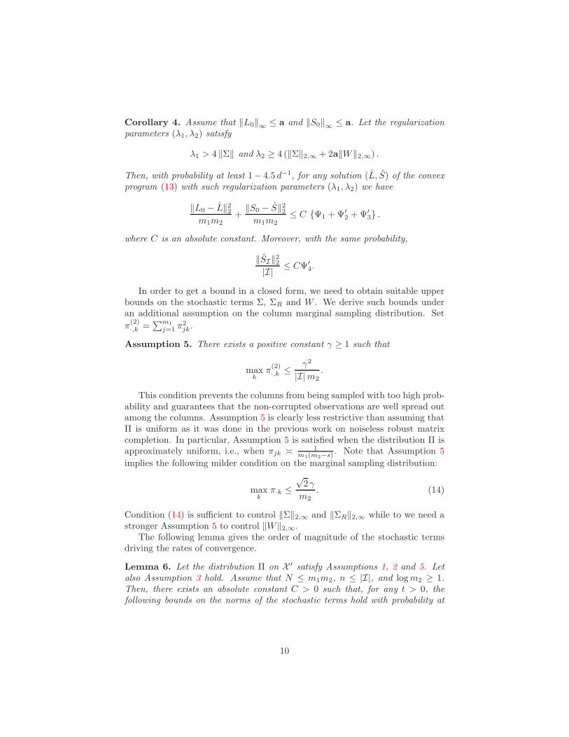
Corollary 4. Assume that ‖L0‖∞ ≤ a and ‖S0‖∞ ≤ a. Let the regularizationparameters (λ1, λ2) satisfy

λ1 > 4 ‖Σ‖ and λ2 ≥ 4 (‖Σ‖2,∞ + 2a‖W‖2,∞) .

Then, with probability at least 1− 4.5 d−1, for any solution (L, S) of the convexprogram (13) with such regularization parameters (λ1, λ2) we have

‖L0 − L‖22m1m2

+‖S0 − S‖22m1m2

≤ C Ψ1 + Ψ′2 + Ψ′

3 .

where C is an absolute constant. Moreover, with the same probability,

‖SI‖22|I| ≤ CΨ′

4.

In order to get a bound in a closed form, we need to obtain suitable upperbounds on the stochastic terms Σ, ΣR and W . We derive such bounds underan additional assumption on the column marginal sampling distribution. Set

π(2)·,k =

∑m1

j=1 π2jk.

Assumption 5. There exists a positive constant γ ≥ 1 such that

maxk

π(2)·,k ≤ γ2

|I|m2.

This condition prevents the columns from being sampled with too high prob-ability and guarantees that the non-corrupted observations are well spread outamong the columns. Assumption 5 is clearly less restrictive than assuming thatΠ is uniform as it was done in the previous work on noiseless robust matrixcompletion. In particular, Assumption 5 is satisfied when the distribution Π isapproximately uniform, i.e., when πjk ≍ 1

m1(m2−s). Note that Assumption 5

implies the following milder condition on the marginal sampling distribution:

maxk

π·k ≤√

2 γ

m2. (14)

Condition (14) is sufficient to control ‖Σ‖2,∞ and ‖ΣR‖2,∞ while to we need astronger Assumption 5 to control ‖W‖2,∞.

The following lemma gives the order of magnitude of the stochastic termsdriving the rates of convergence.

Lemma 6. Let the distribution Π on X ′ satisfy Assumptions 1, 2 and 5. Letalso Assumption 3 hold. Assume that N ≤ m1m2, n ≤ |I|, and logm2 ≥ 1.Then, there exists an absolute constant C > 0 such that, for any t > 0, thefollowing bounds on the norms of the stochastic terms hold with probability at

10

least 1 − e−t, as well as the associated bounds in expectation.

(i) ‖Σ‖ ≤ Cσmax

(√

L(t+ log d)

æNm,

(logm)(t+ log d)

N

)

and

E ‖ΣR‖ ≤ C

(√

L log(d)

nm+

log2 d

N

)

;

(ii) ‖Σ‖2,∞ ≤ Cσ

√

γ(t+ log(d))

æNm2+t+ log d

N

and

E ‖Σ‖2,∞ ≤ Cσ

√

γ log(d)

æNm2+

log d

N

;

(iii) ‖ΣR‖2,∞ ≤ C

√

γ(t+ log(d))

nm2+t+ log d

n

and

E ‖ΣR‖2,∞ ≤ C

√

γ log(d)

nm2+

log d

n

;

(iv) ‖W‖2,∞ ≤ C

γ(t+ logm2)1/4√

æNm2

(

1 +

√

m2(t+ logm2)

n

)1/2

+t+ logm2

N

E‖W‖2,∞ ≤ C

γ log1/4(d)√

æNm2

(

1 +

√

m2 log d

n

)1/2

+log d

N

.

Let

n∗ = 2 log(d)

(m2

γ∨ m log2m

L

)

. (15)

Recall that æ = Nn ≥ 1. If n ≥ n∗, using the bounds given by Lemma 6, we can

chose the regularization parameters λ1 and λ2 in the following way:

λ1 = C (σ ∨ a)

√

L log(d)

Nmand λ2 = C γ (σ ∨ a)

√

log(d)

Nm2, (16)

where C > 0 is a large enough numerical constant.With this choice of the regularization parameters, Corollary 4 implies the

following result.

Corollary 7. Let the distribution Π on X ′ satisfy Assumptions 1, 2 and 5. LetAssumption 3 hold and ‖L0‖∞ ≤ a, ‖S0‖∞ ≤ a. Assume that N ≤ m1m2 and

n∗ ≤ n. Then, with probability at least 1 − 6/d for any solution (L, S) of the

11

convex program (13) with the regularization parameters (λ1, λ2) given by (16),we have

‖L0 − L‖22m1m2

+‖S0 − S‖22m1m2

≤ Cµ,γ,L(σ ∨ a)2 log(d) ærM + |Ω|

n+

a2s

m2

(17)

where Cµ,γ,L > 0 can depend only on µ, γ, L. Moreover, with the same proba-bility,

‖SI‖22|I| ≤ Cµ,γ,L

æ(σ ∨ a)2 |Ω| log(d)

n+

a2s

m2.

Remarks. 1. The upper bound (17) can be decomposed into two terms.The first term is proportional to rM/n. It is of the same order as in the caseof the usual matrix completion, see [19, 17]. The second term accounts for thecorruption. It is proportional to the number of corrupted columns s and tothe number of corrupted observations |Ω|. This term vanishes if there is nocorruption, i.e., when S0 = 0.

2. If all entries of A0 are observed, i.e., the matrix decomposition problemis considered, the bound (17) is analogous to the corresponding bound in [1].Indeed, then |Ω| = sm1, N = m1m2, æ ≤ 2 and we get

‖L0 − L‖22m1m2

+‖S0 − S‖22m1m2

. (σ ∨ a)2(

rM

m1m2+

s

m2

)

.

The estimator studied in [1] for matrix decomposition problem is similar toour program (13). The difference between these estimators is that in (13) theminimization is over ‖ · ‖∞-balls while the program of [1] uses the minimizationover ‖ · ‖2,∞-balls and requires the knowledge of a bound on the norm ‖L0‖2,∞of the unknown matrix L0.

3. Suppose that the number of corrupted columns is small (s ≪ m2). Then,Corollary 7 guarantees, that the prediction error of our estimator is small when-ever the number of non-corrupted observations n satisfies the following condition

n & (m1 ∨m2)rank(L0) + |Ω| (18)

where |Ω| is the number of corrupted observations. This quantifies the samplesize sufficient for successful (robust to corruptions) matrix completion. Whenthe rank r of L0 is small and s≪ m2, the right hand side of (18) is considerablysmaller than the total number of entries m1m2.

4. By changing the numerical constants, one can obtain that the upperbound (17) is valid with probability 1 − 6d−α for a given α ≥ 1.

5 Entrywise sparse corruptions

We assume now that S0 has s non-zero entries but they do not necessarily layin a small subset of columns. We will also assume that s ≤ m1m2

2 . We use now

12

the l1-regularizer R. Then the convex program (5) takes the form

(L, S) ∈ arg min‖L‖∞≤a

‖S‖∞≤a

1

N

N∑

i=1

(Yi − 〈Xi, L+ S〉)2 + λ1‖L‖∗ + λ2‖S‖1

. (19)

The support I = (j, k) : (S0)jk 6= 0 of the non-zero entries of S0 satisfies

|I| = s. Also, ‖IdΩ‖1 = |Ω| so that Ψ2, Ψ3, and Ψ4 take form

Ψ′′2 = µ a |Ω|

(aλ2λ1

E (‖ΣR‖) + æλ2 + aE‖ΣR‖2,∞)

,

Ψ′′3 =

µ |Ω|(a2 + σ2 log(d)

)

N

(aE (‖ΣR‖)

λ1+

aE‖ΣR‖2,∞λ2

+ æ

)

+a2s

m1m2,

Ψ′′4 = µ a2

√

log(d)

n+ µ a |Ω| [æλ2 + aE‖ΣR‖2,∞]

+

[aE‖ΣR‖2,∞

λ2+ æ

]µ |Ω|

(a2 + σ2 log(d)

)

N.

Specializing Theorem 1 to this case yields the following corollary:

Corollary 8. Assume that ‖L0‖∞ ≤ a and ‖S0‖∞ ≤ a. Let the regularizationparameters (λ1, λ2) satisfy

λ1 > 4 ‖Σ‖ and λ2 ≥ 4 (‖Σ‖∞ + 2a‖W‖∞) .

Then, with probability at least 1− 4.5 d−1, for any solution (L, S) of the convexprogram (19) with such regularization parameters (λ1, λ2) we have

‖L0 − L‖22m1m2

+‖S0 − S‖22m1m2

≤ C Ψ1 + Ψ′′2 + Ψ′′

3

where C is an absolute constant. Moreover, with the same probability,

‖SI‖22|I| ≤ CΨ′′

4 .

In order to get a bound in a closed form we need to obtain suitable upperbounds on the stochastic terms Σ,ΣR and W . We provide such bounds underthe following additional assumption on the sampling distribution.

Assumption 9. There exists a positive constant γ ≥ 1 such that

maxi,j

πij ≤µ1

|I| .

This assumption prevents any entry from being sampled too often and guar-antees that the observations are well spread out over the non-corrupted entries.Assumptions 1 and 9 imply that the sampling distribution Π is approximatelyuniform in the sense that πjk ≍ 1

|I| . In particular, since |I| ≤ m1m2

2 , Assump-

tion 9 implies Assumption 2 for L = 2µ1.

13

Lemma 10. Let the distribution Π on X ′ satisfy Assumptions 1, and 9. Let alsoAssumption 3 hold. Then, there exists an absolute constant C > 0 such that,for any t > 0, the following bounds on the norms of the stochastic terms holdwith probability at least 1− e−t, as well as the associated bounds in expectation.

(i) ‖W‖∞ ≤ C

µ1

æm1m2+

√

µ1(t+ log d))

æNm1m2+t+ log d

N

and

E‖W‖∞ ≤ C

(

µ1

æm1m2+

√

µ1 log d

æNm1m2+

log d

N

)

;

(ii) ‖Σ‖∞ ≤ Cσ

√

µ1(t+ log d)

æNm1m2+t+ log d

N

and

E ‖Σ‖∞ ≤ Cσ

(√

µ1 log d

æNm1m2+

log d

N

)

;

(iii) ‖ΣR‖∞ ≤ C

√

µ1(t+ log d)

nm1m2+t+ log d

n

and

E ‖ΣR‖∞ ≤ C

(√

µ1 log d

nm1m2+

log d

n

)

.

Using Lemma 6(i), and Lemma 10, under the conditions

m1m2 log d

µ1≥ n ≥ 2m log(d) log2(m)

L(20)

we can choose the regularization parameters λ1 and λ2 in the following way:

λ1 = C(σ ∨ a)

√

µ1 log(d)

Nmand λ2 = C(σ ∨ a)

log(d)

N. (21)

With this choice of the regularization parameters, Corollary 8 and Lemma 10imply the following result.

Corollary 11. Let the distribution Π on X ′ satisfy Assumptions 1, and 9. LetAssumption 3 hold and ‖L0‖∞ ≤ a, ‖S0‖∞ ≤ a. Assume that N ≤ m1m2

and that condition (20) holds. Then, with probability at least 1 − 6/d for anysolution (L, S) of the convex program (19) with the regularization parameters(λ1, λ2) given by (21), we have

‖L0 − L‖22m1m2

+‖S0 − S‖22m1m2

≤ Cµ,µ1æ(σ ∨ a)2 log(d)

rM + |Ω|n

+a2s

m1m2

(22)

where Cµ,µ1> 0 can depend only on µ and µ1. Moreover, with the same proba-

bility

‖SI‖22|I| ≤ Cµ,µ1

æ(σ ∨ a)2|Ω| log(d)

n+

a2s

m1m2.

14

Remarks. 1. As in the columnwise sparsity case, we can recognize twoterms in the upper bound (22). The first term is proportional to rM/n. It is ofthe same order as the rate of convergence for the usual matrix completion, see[19, 17]. The second term accounts for the corruptions and is proportional to thenumber s of nonzero entries in S0 and to the number of corrupted observations|Ω|. We will prove in Section 6 below that these error terms are of the correctorder up to a logarithmic factor.

2. If s ≪ n < m1m2, the bound (22) implies that one can estimate a low-rank matrix from a nearly minimal number of observations, even when a partof the observations has been corrupted.

3. If all entries of A0 are observed, i.e., the matrix decomposition problemis considered, the bound (22) is analogous to the corresponding bound in [1].Indeed, then |Ω| ≤ s,N = m1m2, æ ≤ 2 and we get

‖L0 − L‖22m1m2

+‖S0 − S‖22m1m2

. (σ ∨ a)2(

rM

m1m2+

s

m1m2

)

.

6 Minimax lower bounds

In this section, we prove the minimax lower bounds showing that the ratesattained by our estimator are optimal up to a logarithmic factor. We will denoteby inf(L,S) the infimum over all pairs of estimators (L, S) for the components

L0 and S0 in the decomposition A0 = L0 + S0 where both L and S take valuesin R

m1×m2 . For any A0 ∈ Rm1×m2 , let PA0

denote the probability distributionof the observations (X1, Y1, . . . , Xn, Yn) satisfying (1).

We begin with the case of columnwise sparsity. For any matrix S ∈ Rm1×m2 ,

we denote by ‖S‖2,0 the number of nonzero columns of S. For any integers0 ≤ r ≤ min(m1,m2), 0 ≤ s ≤ m2 and any a > 0, we consider the class ofmatrices

AGS(r, s, a) =A0 = L0 + S0 ∈ R

m1×m2 : rank(L0) ≤ r, ‖L0‖∞ ≤ a,

and ‖S0‖2,0 ≤ s , ‖S0‖∞ ≤ a (23)

and define

ψGS(N, r, s) = (σ ∧ a)2

(

Mr + |Ω|n

+s

m2

)

.

The following theorem gives a lower bound on the estimation risk in the case ofcolumnwise sparsity.

Theorem 2. Suppose that m1,m2 ≥ 2. Fix a > 0 and integers 1 ≤ r ≤min(m1,m2) and 1 ≤ s ≤ m2/2. Let Assumption 9 be satisfied. Assume thatMr ≤ n, |Ω| ≤ sm1 and æ ≤ 1 + s/m2. Suppose that the variables ξi arei.i.d. Gaussian N (0, σ2), σ2 > 0, for i = 1, . . . , n. Then, there exist absoluteconstants β ∈ (0, 1) and c > 0, such that

inf(L,S)

sup(L0,S0)∈AGS(r,s,a)

PA0

(

‖L− L0‖22m1m2

+‖S − S0‖22m1m2

> cψGS(N, r, s)

)

≥ β.

15

We turn now to the case of entrywise sparsity. For any matrix S ∈ Rm1×m2 ,

we denote by ‖S‖0 the number of nonzero entries of S. For any integers 0 ≤ r ≤min(m1,m2), 0 ≤ s ≤ m1m2/2 and any a > 0, we consider the class of matrices

AS(r, s, a) =A0 = L0 + S0 ∈ R

m1×m2 : rank(L0) ≤ r,

‖S0‖0 ≤ s, ‖L0‖∞ ≤ a, ‖S0‖∞ ≤ a

and define

ψS(N, r, s) = (σ ∧ a)2

Mr + |Ω|n

+s

m1m2

.

We have the following theorem for the lower bound in the case of entrywisesparsity.

Theorem 3. Assume that m1,m2 ≥ 2. Fix a > 0 and integers 1 ≤ r ≤min(m1,m2) and 1 ≤ s ≤ m1m2/2. Let Assumption 9 be satisfied. Assume thatMr ≤ n and there exists a constant ρ > 0 such that |Ω| ≤ ρ rM . Suppose thatthe variables ξi are i.i.d. Gaussian N (0, σ2), σ2 > 0, for i = 1, . . . , n. Then,there exist absolute constants β ∈ (0, 1) and c > 0, such that

inf(L,S)

sup(L0,S0)∈AS(r,s,a)

PA0

(‖L− L0‖22m1m2

+‖S − S0‖22m1m2

> cψS(N, r, s)

)

≥ β. (24)

Appendix

A Proofs of Theorem 1 and of Corollary 7

A.1 Proof of Theorem 1

The proofs of the upper bounds have similarities with the methods developed in[17] for noisy matrix completion but the presence of corruptions in our settingrequires a new approach, in particular, for proving ”restricted strong convexityproperty” (Lemma 15) which is the main difficulty in the proof.

Recall that our estimator is defined as

(L, S) ∈ arg min‖L‖∞≤a

‖S‖∞≤a

1

N

N∑

i=1

(Yi − 〈Xi, L+ S〉)2 + λ1‖L‖∗ + λ2R(S)

and our goal is to bound from above the Frobenius norms ‖L0− L‖22 and ‖S0−S‖22.

1) Set F(L, S) = 1N

∑Ni=1 (Yi − 〈Xi, L+ S〉)2 + λ1‖L‖∗ + λ2R(S), ∆L =

L0− L and ∆S = S0 − S. Using the inequality F(L, S) ≤ F(L0, S0) and (1) weget

1

N

N∑

i=1

(〈Xi,∆L+ ∆S〉 + ξi)2+λ1‖L‖∗+λ2R(S) ≤ 1

N

N∑

i=1

ξ2i +λ1‖L0‖∗+λ2R(S0).

16

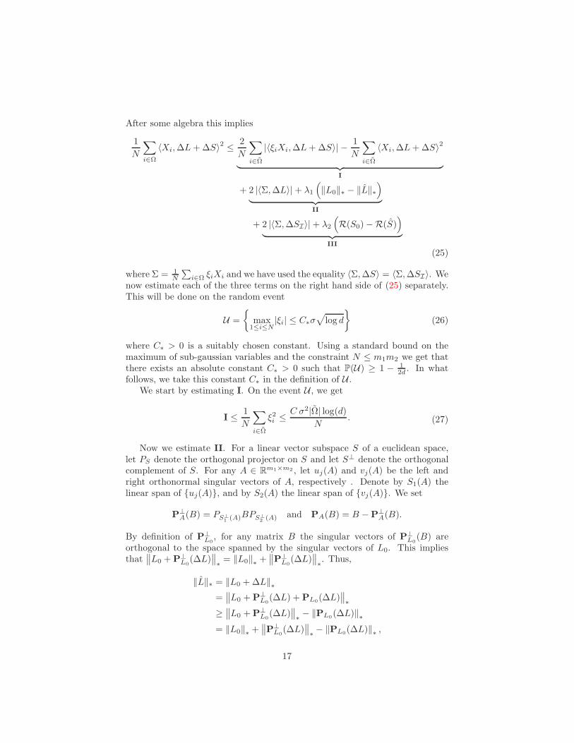
After some algebra this implies

1

N

∑

i∈Ω

〈Xi,∆L+ ∆S〉2 ≤ 2

N

∑

i∈Ω

|〈ξiXi,∆L+ ∆S〉| − 1

N

∑

i∈Ω

〈Xi,∆L+ ∆S〉2

︸ ︷︷ ︸

I

+ 2 |〈Σ,∆L〉| + λ1

(

‖L0‖∗ − ‖L‖∗)

︸ ︷︷ ︸

II

+ 2 |〈Σ,∆SI〉| + λ2

(

R(S0) −R(S))

︸ ︷︷ ︸

III

(25)

where Σ = 1N

∑

i∈Ω ξiXi and we have used the equality 〈Σ,∆S〉 = 〈Σ,∆SI〉. Wenow estimate each of the three terms on the right hand side of (25) separately.This will be done on the random event

U =

max1≤i≤N

|ξi| ≤ C∗σ√

log d

(26)

where C∗ > 0 is a suitably chosen constant. Using a standard bound on themaximum of sub-gaussian variables and the constraint N ≤ m1m2 we get thatthere exists an absolute constant C∗ > 0 such that P(U) ≥ 1 − 1

2d . In whatfollows, we take this constant C∗ in the definition of U .

We start by estimating I. On the event U , we get

I ≤ 1

N

∑

i∈Ω

ξ2i ≤ C σ2|Ω| log(d)

N. (27)

Now we estimate II. For a linear vector subspace S of a euclidean space,let PS denote the orthogonal projector on S and let S⊥ denote the orthogonalcomplement of S. For any A ∈ R

m1×m2 , let uj(A) and vj(A) be the left andright orthonormal singular vectors of A, respectively . Denote by S1(A) thelinear span of uj(A), and by S2(A) the linear span of vj(A). We set

P⊥A(B) = PS⊥

1(A)BPS⊥

2(A) and PA(B) = B −P⊥

A(B).

By definition of P⊥L0

, for any matrix B the singular vectors of P⊥L0

(B) areorthogonal to the space spanned by the singular vectors of L0. This impliesthat

∥∥L0 + P⊥

L0(∆L)

∥∥∗

= ‖L0‖∗ +∥∥P⊥

L0(∆L)

∥∥∗. Thus,

‖L‖∗ = ‖L0 + ∆L‖∗=∥∥L0 + P⊥

L0(∆L) + PL0

(∆L)∥∥∗

≥∥∥L0 + P⊥

L0(∆L)

∥∥∗− ‖PL0

(∆L)‖∗= ‖L0‖∗ +

∥∥P⊥

L0(∆L)

∥∥∗− ‖PL0

(∆L)‖∗ ,

17

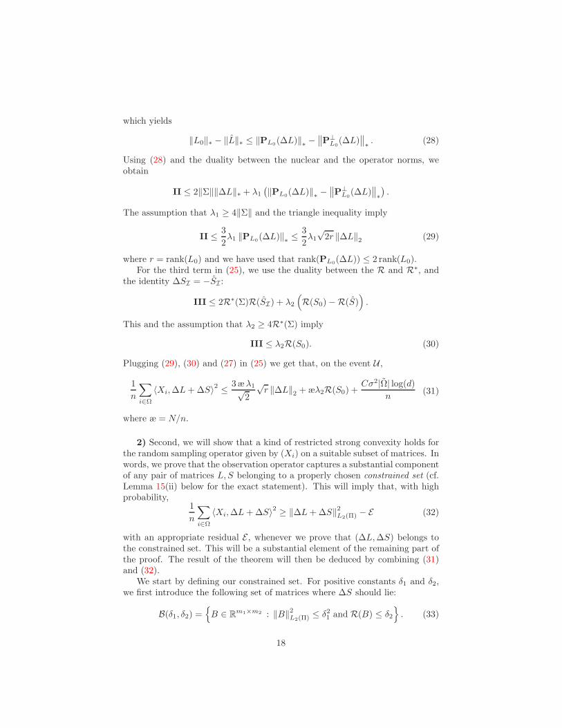
which yields

‖L0‖∗ − ‖L‖∗ ≤ ‖PL0(∆L)‖∗ −

∥∥P⊥

L0(∆L)

∥∥∗. (28)

Using (28) and the duality between the nuclear and the operator norms, weobtain

II ≤ 2‖Σ‖‖∆L‖∗ + λ1(‖PL0

(∆L)‖∗ −∥∥P⊥

L0(∆L)

∥∥∗

).

The assumption that λ1 ≥ 4‖Σ‖ and the triangle inequality imply

II ≤ 3

2λ1 ‖PL0

(∆L)‖∗ ≤ 3

2λ1

√2r ‖∆L‖2 (29)

where r = rank(L0) and we have used that rank(PL0(∆L)) ≤ 2 rank(L0).

For the third term in (25), we use the duality between the R and R∗, andthe identity ∆SI = −SI :

III ≤ 2R∗(Σ)R(SI) + λ2

(

R(S0) −R(S))

.

This and the assumption that λ2 ≥ 4R∗(Σ) imply

III ≤ λ2R(S0). (30)

Plugging (29), (30) and (27) in (25) we get that, on the event U ,

1

n

∑

i∈Ω

〈Xi,∆L+ ∆S〉2 ≤ 3 æλ1√2

√r ‖∆L‖2 + æλ2R(S0) +

Cσ2|Ω| log(d)

n(31)

where æ = N/n.

2) Second, we will show that a kind of restricted strong convexity holds forthe random sampling operator given by (Xi) on a suitable subset of matrices. Inwords, we prove that the observation operator captures a substantial componentof any pair of matrices L, S belonging to a properly chosen constrained set (cf.Lemma 15(ii) below for the exact statement). This will imply that, with highprobability,

1

n

∑

i∈Ω

〈Xi,∆L+ ∆S〉2 ≥ ‖∆L+ ∆S‖2L2(Π) − E (32)

with an appropriate residual E , whenever we prove that (∆L,∆S) belongs tothe constrained set. This will be a substantial element of the remaining part ofthe proof. The result of the theorem will then be deduced by combining (31)and (32).

We start by defining our constrained set. For positive constants δ1 and δ2,we first introduce the following set of matrices where ∆S should lie:

B(δ1, δ2) =

B ∈ Rm1×m2 : ‖B‖2L2(Π) ≤ δ21 and R(B) ≤ δ2

. (33)

18

The constants δ1 and δ2 define the constraints on the L2(Π)-norm and on thesparsity of the component S. The error term E in (32) depends on δ1 and δ2.We will specify the suitable values of δ1 and δ2 for the matrix ∆S later. Next,we define the following set of pairs of matrices:

D(τ, κ) =

(A,B) ∈ Rm1×m2 : ‖A+B‖2L2(Π) ≥

√

64 log(d)

log (6/5) n,

‖A+B‖∞ ≤ 1, ‖A‖∗ ≤ √τ ‖AI‖2 + κ

where κ and τ < m1 ∧ m2 are some positive constants. This will be usedfor A = ∆L and B = ∆S. If the L2(Π)-norm of the sum of two matrices istoo small, the right hand side of (32) is negative. The first inequality in thedefinition of D(τ, κ) prevents from this. Condition ‖A‖∗ ≤ √

τ ‖AI‖2 + κ is arelaxed form of the condition ‖A‖∗ ≤ √

τ ‖A‖2 satisfied by matrices with rank τ .We will show that, with high probability, the matrix ∆L satisfies this conditionwith τ = C rank(L0) and a small κ. To prove it, we need the bound R(B) ≤ δ2on the corrupted part.

Finally, define our constrained set as the intersection

D(τ, κ) ∩Rm1×m2 × B(δ1, δ2)

.

We now return to the proof of the theorem. To prove (11), we bound sepa-rately the norms ‖∆L‖2 and ‖∆S‖2. Note that

‖∆L‖22 ≤ ‖∆LI‖22 + ‖∆LI‖22 ≤ ‖∆LI‖22 + 4a2|I|≤ µ|I|‖∆LI‖2L2(Π) + 4a2|I|

(34)

and similarly,

‖∆S‖22 ≤ µ|I|‖∆SI‖2L2(Π) + 4a2|I|.

In view of these inequalities, it is enough to bound the quantities ‖∆SI‖2L2(Π)

and ‖∆LI‖22. A bound on ‖∆SI‖2L2(Π) with the rate as claimed in (11) is given

in Lemma 14 below. In order to bound ‖∆LI‖2L2(Π) (or ‖∆LI‖22 according to

cases), we will need the following argument.

Case 1: Suppose that ‖∆L + ∆S‖2L2(Π) < 16a2

√

64 log(d)

log (6/5) n. Then a

straightforward inequality

‖∆L+ ∆S‖2L2(Π) ≥1

2‖∆L‖2L2(Π) − ‖∆S‖2L2(Π) (35)

together with Lemma 14 below implies that, with probability at least 1− 2.5/d,

‖∆L‖2L2(Π) ≤ ∆1 (36)

19

where

∆1 = CΨ4/µ = C

a2√

log(d)

n+ aR(IdΩ) [æλ2 + aE (R∗(ΣR))]

+

(aE (R∗(ΣR))

λ2+ æ

) |Ω|(a2 + σ2 log(d)

)

N

.

Note also that Ψ4 ≤ C(Ψ1 + Ψ2 + Ψ3). In view of (34), (36) and of fact that|I| ≤ m1m2, the bound on ‖∆L‖22 stated in the theorem holds with probabilityat least 1 − 2.5/d.

Case 2: Assume now that ‖∆L+ ∆S‖2L2(Π) ≥ 16a2

√

64 log(d)

log (6/5) n. We will

show that in this case and with an appropriate choice of δ1, δ2, τ and κ, the pair14a(∆L,∆S) belongs to the intersection D(τ, κ) ∩ Rm1×m2 × B(δ1, δ2).

Lemma 13 below and (27) imply that, on the event U ,

‖∆L‖∗ ≤ 4√

2r‖∆L‖2 +λ2 a

λ1R(IdΩ) +

Cσ2|Ω| log(d)

Nλ1

≤ 4√

2r‖∆LI‖2 + 8a

√

2r|I| +λ2 a

λ1R(IdΩ) +

Cσ2|Ω| log(d)

Nλ1.

(37)

Lemma 14 yields that, with probability at least 1 − 2.5 d−1,

∆S

4a∈ B

(√∆1

4a, 2R(IdΩ) +

C|Ω|(a2 + σ2 log(d)

)

4aNλ2

)

= B.

This property and (37) imply that 14a (∆L,∆S) ∈ D(τ, κ)∩

Rm1×m2 × B

with

probability at least 1 − 2.5 d−1, where

τ = 32r and κ = 2

√

2r|I| +λ24λ1

R(IdΩ) +Cσ2|Ω| log(d)

4aNλ1.

Therefore, we can apply Lemma 15(ii). From Lemma 15(ii) and (31) we obtainthat, with probability at least 1 − 4.5 d−1,

1

2‖∆L+ ∆S‖2L2(Π) ≤

3 æλ1√2

√r ‖∆L‖2 + CE (38)

where

E = µ a2 r |I| (E (‖ΣR‖))2

+ 8a2√

2r|I|E (‖ΣR‖) + λ2R(IdΩ)

(a2E (‖ΣR‖)

λ1+ aæ

)

+|Ω|(a2 + σ2 log(d)

)

N

(aE (‖ΣR‖)

λ1+

aE (R∗(ΣR))

λ2+ æ

)

+ ∆1.

(39)

20

Using an elementary argument and then (34) we find

3 æ√2λ1

√r ‖∆L‖2 ≤ 9 æ2 µm1m2 r λ

21

2+

‖∆L‖224µm1m2

≤ 9 æ2 µm1m2 r λ21

2+

‖∆LI‖224µm1m2

+a2|I|µm1m2

.

This inequality and (38) yield

‖∆L+ ∆S‖2L2(Π) ≤9 æ2 µm1m2 r λ

21

4+

‖∆LI‖224µm1m2

+a2|I|µm1m2

+ CE .

Using again (35), Lemma 14, (9) and the bound |I| ≤ m1m2 we obtain

‖∆LI‖22µm1m2

≤ C

æ2 µm1m2 r λ21 +

a2|I|µm1m2

+ E

.

This and the inequality√

2r|I|E (‖ΣR‖) ≤ |I|µm1m2

+ µm1m2 r (E (‖ΣR‖))2

imply that, with probability at least 1 − 4.5 d−1,

‖∆LI‖22m1m2

≤ C Ψ1 + Ψ2 + Ψ3 . (40)

In view of (40) and (34), ‖∆L‖22 is bounded by the right hand side of (11) withprobability at least 1− 4.5 d−1. Finally, inequality (12) follows from Lemma 14,(9) and the identity ∆SI = −SI .

Lemma 12. Assume that λ2 ≥ 4 (R∗(Σ) + 2aR∗(W )). Then, we have

R(∆SI) ≤ 3R(∆SΩ) +1

Nλ2

4a2|Ω| +∑

i∈Ω

ξ2i

Proof. Let ∂‖ · ‖∗, and ∂R denote the subdifferentials of ‖ · ‖∗ and of R, re-spectively. By the standard condition for optimality over a convex set (see [2],Chapter 4, Section 2, Corollary 6), we have

− 2

N

N∑

i=1

(

Yi −⟨

Xi, L+ S⟩)⟨

Xi, L+ S − L− S⟩

+ λ1

⟨

∂‖L‖∗, L− L⟩

+ λ2

⟨

∂R(S), S − S⟩

≥ 0

(41)

for all feasible pairs (L, S). In particular, for (L, S0) we obtain

− 2

N

N∑

i=1

(

Yi −⟨

Xi, L+ S⟩)

〈Xi,∆S〉 + λ2

⟨

∂R(S),∆S⟩

≥ 0,

21

which implies

− 2

N

N∑

i=1

〈Xi,∆S〉2 −2

N

∑

i∈Ω

〈Xi,∆L〉 〈Xi,∆S〉 −2

N

∑

i∈Ω

ξi 〈Xi,∆S〉

− 2

N

∑

i∈Ω

〈Xi,∆L〉 〈Xi,∆S〉 − 2 〈Σ,∆S〉 + λ2

⟨

∂R(S),∆S⟩

≥ 0.

Using the elementary inequality 2ab ≤ a2 + b2 and the bound ‖∆L‖∞ ≤ 2a wefind

− 2

N

N∑

i=1

〈Xi,∆S〉2 −2

N

∑

i∈Ω

〈Xi,∆L〉 〈Xi,∆S〉 −2

N

∑

i∈Ω

ξi 〈Xi,∆S〉

≤ 1

N

∑

i∈Ω

〈Xi,∆L〉2 +1

N

∑

i∈Ω

ξ2

≤ 4a2|Ω|N

+1

N

∑

i∈Ω

ξ2i .

Combining the last two displays we get

λ2

⟨

∂R(S), S − S0

⟩

≤ 2

∣∣∣∣∣

⟨

1

N

∑

i∈Ω

〈Xi,∆L〉Xi,∆S

⟩∣∣∣∣∣

+ 2 |〈Σ,∆S〉| +4a2|Ω|N

+1

N

∑

i∈Ω

ξ2i

≤ 2R∗

(

1

N

∑

i∈Ω

〈Xi,∆L〉Xi

)

R(∆S) + 2R∗(Σ)R(∆S)

+4a2|Ω|N

+1

N

∑

i∈Ω

ξ2i .

(42)

By Lemma 18,

R∗

(

1

N

∑

i∈Ω

〈Xi,∆L〉Xi

)

≤ 2aR∗(W ) (43)

where W = 1N

∑

i∈ΩXi. On the other hand, the convexity of R(·) and thedefinition of subdifferential imply

R(S0) ≥ R(S) +⟨

∂R(S),∆S⟩

. (44)

Plugging (43) and (44) in (42) we obtain

λ2

(

R(S) −R(S0))

≤ 4aR∗(W )R(∆S) + 2R∗(Σ)R(∆S) +4a2|Ω|N

+1

N

∑

i∈Ω

ξ2i .

22

Next, the decomposability of R(·), the identity (S0)I = 0 and the triangleinequality yield

R(S0 − ∆S) −R(S0) = R ((S0 − ∆S)I) + R ((S0 − ∆S)I) −R ((S0)I)

≥ R ((∆S)I) −R ((∆S)I) .

Since λ2 ≥ 4 (2aR∗(W ) + R∗(Σ)) the last two displays imply

λ2 (R ((∆S)I) −R ((∆S)I))

≤ λ22

(R (∆SI) + R ((∆S)I)) +4a2|Ω|N

+1

N

∑

i∈Ω

ξ2i .

Thus,

R (∆SI) ≤ 3R (∆SI) +1

Nλ2

4a2|Ω| +∑

i∈Ω

ξ2i

. (45)

Since we assume that all unobserved entries of S0 are zero, we have (S0)I =

(S0)Ω. On the other hand, SI = SΩ as R(·) is a monotonic norm. Indeed, addingto S a non-zero element on the non-observed part increases R(S) but does not

modify 1N

∑Ni=1 (Yi − 〈Xi, L+ S〉)2. To conclude, we have ∆SI = ∆SΩ, which

together with (45), implies the Lemma.

Lemma 13. Suppose that λ1 ≥ 4‖Σ‖ and λ2 ≥ 4R∗(Σ). Then,

∥∥P⊥

L0(∆L)

∥∥∗≤ 3 ‖PL0

(∆L)‖∗ +λ2 a

λ1R(IdΩ) +

1

Nλ1

∑

i∈Ω

ξ2i .

Proof. Using (41) for (L, S) = (L0, S0) we obtain

− 2

N

N∑

i=1

〈Xi,∆S + ∆L〉2 − 2

N

∑

i∈Ω

〈ξiXi,∆L + ∆S〉

− 2 〈Σ, (∆S)I〉 − 2 〈Σ,∆L〉 + λ1

⟨

∂‖L‖∗,∆L⟩

+ λ2

⟨

∂R(S),∆S⟩

≥ 0.

(46)

The convexity of ‖·‖∗ and of R(·) and the definition of the subdifferential imply

‖L0‖∗ ≥ ‖L‖∗ +⟨

∂‖L‖∗,∆L⟩

R(S0) ≥ R(S) +⟨

∂R(S),∆S⟩

.

Together with (46), this yields

λ1

(

‖L‖∗ − ‖L0‖∗)

+ λ2

(

R(S) −R(S0))

≤ 2‖Σ‖‖∆L‖∗ + 2R∗(Σ)R (∆SI)

+1

N

∑

i∈Ω

ξ2i .

23

Using the conditions λ1 ≥ 4‖Σ‖, λ2 ≥ 4R∗(Σ), the triangle inequality and (28)we get

λ1(∥∥P⊥

L0(∆L)

∥∥∗− ‖PL0

(∆L)‖∗)

+ λ2

(

R(S) −R(S0))

≤ λ12

(∥∥P⊥

L0(∆L)

∥∥∗

+ ‖PL0(∆L)‖∗

)+λ22R(

SI

)

+1

N

∑

i∈Ω

ξ2i .

Since we assume that all unobserved entries of S0 are zero, we obtain R(S0) ≤aR(IdΩ). Using this inequality in the last display proves the lemma.

Lemma 14. Let n > m1 and λ2 ≥ 4 (R∗(Σ) + 2aR∗(W )). Suppose that thedistribution Π on X ′ satisfies Assumptions 1 and 2. Let ‖S0‖∞ ≤ a for someconstant a and let Assumption 3 be satisfied. Then, with probability at least1 − 2.5 d−1,

‖∆S‖2L2(Π) ≤ CΨ4/µ, (47)

and

R(∆S) ≤ 8aR(IdΩ) +|Ω|(4a2 + Cσ2 log(d)

)

Nλ2. (48)

Proof. Using the inequality F(L, S) ≤ F(L, S0) and (1) we obtain

1

N

N∑

i=1

(〈Xi,∆L+ ∆S〉 + ξi)2 + λ2R(S)

≤ 1

N

N∑

i=1

(〈Xi,∆L〉 + ξi)2

+ λ2R(S0)

which implies

1

N

∑

i∈Ω

〈Xi,∆S〉2 +1

N

∑

i∈Ω

〈Xi,∆S〉2 +2

N

∑

i∈Ω

〈Xi,∆L〉 〈Xi,∆S〉 +2

N

∑

i∈Ω

〈ξiXi,∆S〉

+2

N

∑

i∈Ω

〈Xi,∆L〉 〈Xi,∆SI〉 + 2 〈Σ,∆SI〉 + λ2R(S) ≤ λ2R(S0).

From Lemma 18 and the duality between R and R∗ we obtain

1

N

∑

i∈Ω

〈Xi,∆S〉2 ≤ 2 (2aR∗(W ) + R∗(Σ))R(∆SI) + λ2

(

R(S0) −R(S))

+2

N

∑

i∈Ω

〈Xi,∆L〉2 +2

N

∑

i∈Ω

ξ2.

24

Since here ∆SI = −SI and λ2 ≥ 4 (R∗(Σ) + 2aR∗(W )) it follows that

1

N

∑

i∈Ω

〈Xi,∆S〉2 ≤ λ2R (S0) +2

N

∑

i∈Ω

〈Xi,∆L〉2 +2

N

∑

i∈Ω

ξ2. (49)

Now, Lemma 12 and the bound ‖∆S‖∞ ≤ 2a imply that, on the event U definedin (26),

R(∆S) ≤ 4R(∆SΩ) +|Ω|(4a2 + Cσ2 log(d)

)

Nλ2

≤ 8aR(IdΩ) +|Ω|(4a2 + Cσ2 log(d)

)

Nλ2.

(50)

Thus, (48) is proved. To prove (47), consider the following two cases.

Case I: ‖∆S‖2L2(Π) < 4a2√

64 log(d)log(6/5)n . Then (47) holds trivially.

Case II: ‖∆S‖2L2(Π) ≥ 4a2√

64 log(d)log(6/5)n . Then inequality (50) and the bound

‖∆S‖∞ ≤ 2a imply that, on the event U ,

∆S

2a∈ C

(

4R(IdΩ) +|Ω|(8a2 + Cσ2 log(d)

)

2aNλ2

)

where, for any δ > 0, the set C(δ) is defined as:

C(δ) =

A ∈ Rm1×m2 : ‖A‖∞ ≤ 1, ‖A‖2L2(Π) ≥

√

64 log(d)

log (6/5) n,R(A) ≤ δ

.

(51)Thus, we can apply Lemma 15(i) below. In view of this lemma, the inequalities(49), (27), ‖∆L‖∞ ≤ 2a and R (S0) ≤ aR(IdI) imply that (47) holds withprobability at least 1 − 2.5 d−1.

Lemma 15. Let the distribution Π on X ′ satisfy Assumptions 1 and 2. Letδ, δ1, δ2, τ , and κ be positive constants. Then, the following properties hold.

(i) With probability at least 1 − 2

d,

1

n

∑

i∈Ω

〈Xi, S〉2 ≥ 1

2‖S‖2L2(Π) − 8δE (R∗(ΣR))

for any S ∈ C(δ).

(ii) With probability at least 1 − 2

d,

1

n

∑

i∈Ω

〈Xi, L+ S〉2 ≥ 1

2‖L+ S‖2L2(Π) −

360µ |I| τ (E (‖ΣR‖))2

+4δ21 + 8δ2 E (R∗(ΣR)) + 8κE (‖ΣR‖)

for any pair (L, S) ∈ D(τ, κ) ∩ Rm1×m2 × B(δ1, δ2).

25

Proof. We give a unified proof of (i) and (ii). Let A = S for (i) and A = L+ Sfor (ii). Set

E =

8δE (R∗(ΣR)) for (i)

360µ |I| τ (E (‖ΣR‖))2

+ 4δ21 + 8δ2 E (R∗(ΣR)) + 8κE (‖ΣR‖) for (ii)

and

C =

C(δ) for (i)D(τ, κ) ∩ (Rm1×m2 × B(δ1, δ2)) for (ii).

To prove the lemma it is enough to show that the probability of the randomevent

B =

∃A ∈ C such that

∣∣∣∣∣

1

n

∑

i∈Ω

〈Xi, A〉2 − ‖A‖2L2(Π)

∣∣∣∣∣>

1

2‖A‖2L2(Π) + E

is smaller than 2/d. In order to estimate the probability of B, we use a standard

peeling argument. Set ν =

√

64 log(d)

log (6/5) nand α =

6

5. For l ∈ N, define

Sl =

A ∈ C : αl−1ν ≤ ‖A‖2L2(Π) ≤ αlν

.

If the event B holds, there exist l ∈ N and a matrix A ∈ C ∩ Sl such that∣∣∣∣∣

1

n

∑

i∈Ω

〈Xi, A〉2 − ‖A‖2L2(Π)

∣∣∣∣∣>

1

2‖A‖2L2(Π) + E

>1

2αl−1ν + E

=5

12αlν + E .

(52)

For each l ∈ N, consider the random event

Bl =

∃A ∈ C′(αlν) :

∣∣∣∣∣

1

n

∑

i∈Ω

〈Xi, A〉2 − ‖A‖2L2(Π)

∣∣∣∣∣>

5

12αlν + E

whereC′(T ) =

A ∈ C : ‖A‖2L2(Π) ≤ T

, ∀T > 0.

Note that A ∈ Sl implies that A ∈ C′(αlν). This and (52) grant the inclusionB ⊂ ∪∞

l=1 Bl. By Lemma 16, P (Bl) ≤ exp(−c5 nα2lν2) where c5 = 1/128. Usingthe union bound we find

P (B) ≤∞

Σl=1

P (Bl)

≤∞

Σl=1

exp(−c5 nα2l ν2)

≤∞

Σl=1

exp(−(2 c5 n log(α) ν2

)l)

26

where we have used the inequality ex ≥ x. We finally obtain, for ν =

√

64 log(d)

log (6/5) n,

P (B) ≤ exp(−2 c5 n log(α) ν2

)

1 − exp (−2 c5 n log(α) ν2)=

exp (− log(d))

1 − exp (− log(d)).

Let

ZT = supA∈C′(T )

∣∣∣∣∣

1

n

∑

i∈Ω

〈Xi, A〉2 − ‖A‖2L2(Π)

∣∣∣∣∣.

Lemma 16. Let the distribution Π on X ′ satisfy Assumptions 1 and 2. Then,

P

(

ZT >5

12T + E

)

≤ exp(−c5 nT 2)

where c5 =1

128.

Proof. We follow a standard approach: first we show that ZT concentratesaround its expectation and then we bound from above the expectation. Since‖A‖∞ ≤ 1 for all A ∈ C′(T ), we have |〈Xi, A〉| ≤ 1. We use first a Talagrandtype concentration inequality, cf. [4, Theorem 14.2], implying that

P

(

ZT ≥ E (ZT ) +1

9

(5

12T

))

≤ exp(−c5 nT 2

)(53)

where c5 =1

128. Next, we bound the expectation E (ZT ). By a standard

symmetrization argument (see e.g. [18, Theorem 2.1]) we obtain

E (ZT ) = E

(

supA∈C′(T )

∣∣∣∣∣

1

n

∑

i∈Ω

〈Xi, A〉2 − E

(

〈X,A〉2)∣∣∣∣∣

)

≤ 2E

(

supA∈C′(T )

∣∣∣∣∣

1

n

∑

i∈Ω

ǫi 〈Xi, A〉2∣∣∣∣∣

)

where ǫini=1 is an i.i.d. Rademacher sequence. Then, the contraction inequal-ity (see e.g. [18]) yields

E (ZT ) ≤ 8E

(

supA∈C′(T )

∣∣∣∣∣

1

n

∑

i∈Ω

ǫi 〈Xi, A〉∣∣∣∣∣

)

= 8E

(

supA∈C′(T )

|〈ΣR, A〉|)

where ΣR =1

n

n∑

i=1

ǫiXi. Now, to obtain a bound on E

(

supA∈C′(T )

|〈ΣR, A〉|)

we will

consider separately the cases C = C(δ) and C = D(τ, κ)∩Rm1×m2 × B(δ1, δ2).

27

Case I: A ∈ C(δ) and ‖A‖2L2(Π) ≤ T . By the definition of C(δ) we have

R(A) ≤ δ. Thus, by the duality between R and R∗,

E (ZT ) ≤ 8E

(

supR(A)≤δ

|〈ΣR, A〉|)

≤ 8δE (R∗(ΣR)) .

This and the concentration inequality (53) imply

P

(

ZT >5

12T + E

)

≤ exp(−c5 nT 2)

with c5 =1

128and E = 8δ E (R∗(ΣR)) as stated.

Case II: A = L + S where (L, S) ∈ D(τ, κ), S ∈ B(δ1, δ2), and ‖L +S‖2L2(Π) ≤ T . Then, by the definition of B(δ1, δ2), we have R(S) ≤ δ2. On the

other hand, the definition of D(τ, κ) yields

‖L‖∗ ≤ √τ‖LI‖2 + κ

and‖L‖L2(Π) ≤ ‖L+ S‖L2(Π) + ‖S‖L2(Π) ≤

√T + δ1.

The last two inequalities imply

‖L‖∗ ≤√

µ |I| τ (√T + δ1) + κ := Γ1.

Therefore we can write

E

(

supA∈C′(T )

|〈ΣR, A〉|)

≤ 8E

(

sup‖L‖∗≤Γ1

|〈ΣR, L〉| + supR(S)≤δ2

|〈ΣR, S〉|)

≤ 8 Γ1 E (‖ΣR‖) + δ2 E (R∗(ΣR)) .

Combining this bound with the following elementary inequalities:

1

9

(5

12T

)

+ 8√

µ |I| τ T E (‖ΣR‖) ≤(

1

9+

8

9

)5

12T + 44µ |I| τ (E (‖ΣR‖))

2,

δ1√

µ |I| τ ,E (‖ΣR‖) ≤ µ |I| τ (E (‖ΣR‖))2

+δ212

and using the concentration bound (53) we obtain

P

(

ZT >5

12T + E

)

≤ exp(−c5 nT 2)

with c5 =1

128and

E = 360µ |I| τ (E (‖ΣR‖))2

+ 4δ21 + 8δ2 E (R∗(ΣR)) + 8κE (‖ΣR‖) (54)

as stated.

28

A.2 Proof of Corollary 7

With λ1 and λ2 given by (16) we obtain

Ψ1 = µ2æ2(σ ∨ a)2M r log d

N,

Ψ′2 ≤ µ2æ2(σ ∨ a)2 log(d)

|Ω|N

+a2s

m2,

Ψ′3 =

µæ|Ω|(a2 + σ2 log(d)

)

N+

a2s

m2

Ψ′4 ≤ µæ2|Ω|

(a2 + σ2 log(d)

)

N+ a2

√

log(d)

n+

a2s

m2.

B Proof of Theorems 2 and 3

Note that the assumption æ ≤ 1 + s/m2 implies that

|Ω|n

≤ s

m2. (55)

Assume w.l.o.g. that m1 ≥ m2. For a γ ≤ 1, define

L =

L = (lij) ∈ Rm1×r : lij ∈

0, γ(σ∧a)(rM

n

)1/2

, ∀1 ≤ i ≤ m1, 1 ≤ j ≤ r

,

and consider the associated set of block matrices

L =

L = ( L · · · L O ) ∈ Rm1×m2 : L ∈ L

,

where O denotes the m1×(m2−r⌊m2/(2r)⌋) zero matrix, and ⌊x⌋ is the integerpart of x.

We define similarly the set of matrices

S =

S = (sij) ∈ Rm1×s : sij ∈

0, γ(σ ∧ a)

, ∀1 ≤ i ≤ m1, 1 ≤ j ≤ s

,

andS =

S = ( O S ) ∈ Rm1×m2 : S ∈ S

,

where O is the m1 × (m2 − s) zero matrix. We now set

A = A = L+ S : L ∈ L, S ∈ S .

Remark 1. In the case m1 < m2, we only need to change the constructionof the low rank component of the test set. We first introduce a matrix L =(L O

)∈ R

r×m2 where L ∈ Rr×(m2/2) with entries in

0, γ(σ ∧ a)(rMn

)1/2

29

and then we replicate this matrix to obtain a block matrix L of size m1 ×m2

L =

L

...

L

O

.

By construction, any element of A as well as the difference of any two ele-ments of A can be decomposed into a low rank component L of rank at most rand a group sparse component S with at most s nonzero columns. In addition,the entries of any matrix in A take values in [0, a]. Thus, A ⊂ AGS(r, s, a).

We first establish a lower bound of the order rM/n. Let A ⊂ A be suchthat for any A = L+S ∈ A we have S = 0. The Varshamov-Gilbert bound (cf.Lemma 2.9 in [25]) guarantees the existence of a subset A0 ⊂ A with cardinalityCard(A0) ≥ 2(rM)/8 + 1 containing the zero m1 ×m2 matrix 0 and such that,for any two distinct elements A1 and A2 of A0,

‖A1 −A2‖22 ≥ Mr

8

(

γ2(σ ∧ a)2Mr

n

)⌊m2

r

⌋

≥ γ2

16(σ ∧ a)2m1m2

Mr

n. (56)

Since ξi ∼ N (0, σ2) we get that, for any A ∈ A0, the Kullback-Leiblerdivergence K

(P0,PA

)between P0 and PA satisfies

K(P0,PA

)=

|Ω|2σ2

‖A‖2L2(Π) ≤µ1γ

2Mr

2(57)

where we have used Assumption 9. From (57) we deduce that the condition

1

Card(A0) − 1

∑

A∈A0

K(P0,PA) ≤ 1

16log(Card(A0) − 1

)(58)

is satisfied if γ > 0 is chosen as a sufficiently small numerical constant. In viewof (56) and (58), the application of Theorem 2.5 in [25] implies

inf(L,S)

sup(L0,S0)∈AGS(r,s,a)

PA0

(

‖L− L0‖22m1m2

+‖S − S0‖22m1m2

>C(σ ∧ a)2Mr

n

)

≥ β

(59)for some absolute constants β ∈ (0, 1).

We now prove the lower bound relative to the corruptions. Let A ⊂ A suchthat for any A = L+S ∈ A we have L = 0. The Varshamov-Gilbert bound (cf.Lemma 2.9 in [25]) guarantees the existence of a subset A0 ⊂ A with cardinalityCard(A0) ≥ 2(sm1)/8 + 1 containing the zero m1 ×m2 matrix 0 and such that,for any two distinct elements A1 and A2 of A0,

‖S1 − S2‖22 ≥ sm1

8

(γ2(σ ∧ a)2

)=γ2 (σ ∧ a)2 s

8m2m1m2. (60)

30

For any A ∈ A0, the Kullback-Leibler divergence between P0 and PA satisfies

K(P0,PA

)=

|Ω|2σ2

γ2(σ ∧ a)2 ≤ γ2m1s

2

which implies that condition (58) is satisfied if γ > 0 is chosen small enough.Thus, applying Theorem 2.5 in [25] we get

inf(L,S)

sup(L0,S0)∈AGS(r,s,a)

PA0

(

‖L− L0‖22m1m2

+‖S − S0‖22m1m2

>C(σ ∧ a)2 s

m2

)

≥ β

(61)for some absolute constant β ∈ (0, 1). Theorem 2 follows from inequalities (55),(59) and (61).

The proof of Theorem 3 follows the same lines as that of Theorem 2. Theonly difference is that we replace S by the following set

S = (sij) ∈ Rm1×m2 : sij ∈

0, γ(σ∧a)

, ∀1 ≤ i ≤ m1, ⌊m2/2⌋+1 ≤ j ≤ m2

.

We omit further details here.

C Proof of Lemma 6

Part (i) of Lemma 6 is proved in Lemmas 5 and 6 in [17].Proof of (ii). For the sake of brevity, we set Xi(j, k) = 〈Xi, ej(m1)ek(m2)⊤〉.

By definition of Σ and ‖ · ‖2,∞, we have

‖Σ‖22,∞ = max1≤k≤m2

m1∑

j=1

(

1

N

∑

i∈Ω

ξiXi(j, k)

)2

.

For any fixed k, we have

m1∑

j=1

(

1

N

∑

i∈Ω

ξiXi(j, k)

)2

=1

N2

∑

i1,i2∈Ω

ξi1ξi2

m1∑

j=1

Xi1(j, k)Xi2(j, k)

= Ξ⊤AkΞ, (62)

where Ξ = (ξ1, · · · , ξn)⊤ and Ak ∈ R|Ω|×|Ω| with entries

ai1i2(k) =1

N2

m1∑

j=1

Xi1(j, k)Xi2 (j, k).

We freeze the Xi and we apply the version of Hanson–Wright inequality in [24]to get that there exists a numerical constant C such that with probability atleast 1 − e−t

∣∣Ξ⊤AkΞ − E[Ξ⊤AkΞ|Xi]

∣∣ ≤ Cσ2

(

‖Ak‖2√t+ ‖Ak‖t

)

. (63)

31

Next, we note that

‖Ak‖22 =∑

i1,i2

a2i1i2(k) ≤ 1

N4

∑

i1i2

m1∑

j1=1

X2i1(j1, k)

m1∑

j1=1

X2i2(j1, k)

≤ 1

N4

∑

i1

m1∑

j1=1

X2i1(j1, k)

2

=

1

N2

∑

i1

m1∑

j1=1

Xi1(j1, k)

2

,

where we have used the Cauchy - Schwarz inequality in the first line and therelation X2

i (j, k) = Xi(j, k).Note that Zi(k) :=

∑m1

j=1Xi(j, k) follows a Bernoulli distribution with pa-rameter π·k and consequently Z(k) =

∑

i∈Ω Zi(k) follows a Binomial distribu-tion B(|Ω|, π·k). We apply Bernstein’s inequality (see, e.g., [4], page 486) to getthat, for any t > 0,

P

(

|Z(k) − E[Z(k)]| ≥ 2√

|Ω|π·kt+ t)

≤ 2e−t.

Consequently, we get with probability at least 1 − 2e−t that

‖Ak‖22 ≤(

|Ω|π·k + 2√

|Ω|π·kt+ t

N2

)2

and, using ‖Ak‖ ≤ ‖Ak‖2, that

‖Ak‖ ≤ |Ω|π·k + 2√

|Ω|π·kt+ t

N2.

Note also that

E[Ξ⊤AkΞ|Xi] =σ2

N2Z(k).

Combining the last three displays with (63) we get, up to a rescaling of theconstants, with probability at least 1 − e−t that

m1∑

j=1

(

1

N

∑

i∈Ωr

ξiXi(j, k)

)2

≤ Cσ2

N2

(

|Ω|π·k + 2√

|Ω|π·kt+ t)

(1 +√t+ t).

Replacing t by t+ logm2 in the above display and using the union bound givesthat, with probability at least 1 − e−t,

‖Σ‖2,∞ ≤ Cσ

N

(

|Ω|π·k + 2√

|Ω|π·k(t+ logm2) + (t+ logm2))1/2

× (1 +√

t+ logm2 + t+ logm2)1/2

= Cσ

N

(√

|Ω|π·k +√

t+ logm2

)(

1 +√

t+ logm2

)

.

32

Assuming that logm2 ≥ 1 we get with probability at least 1 − e−t that

‖Σ‖2,∞ ≤ Cσ

N

(√

|Ω|π·k(t+ logm2) + (t+ logm2))

.

Using (14), we get that there exists a numerical constant C > 0 such withprobability at least 1 − e−t

‖Σ‖2,∞ ≤ Cσ

N

√

γ1/2n(t+ logm2)

m2+ (t+ logm2)

.

Finally, we use Lemma 17 to obtain the required bound on E‖Σ‖2,∞.Proof of (iii). We follow the same lines as in the proof of part (ii) above.

The only difference is to replace ξi by ǫi, σ by 1 and N by n.Proof of (iv). We need to establish the bound on

‖W‖22,∞ = max1≤k≤m2

m1∑

j=1

(

1

N

∑

i∈Ω

Xi(j, k)

)2

.

For any fixed k, we have

m1∑

j=1

(

1

N

∑

i∈Ω

Xi(j, k)

)2

=1

N2

∑

i∈Ω

m1∑

j=1

X2i (j, k) +

1

N2

∑

i1 6=i2

m1∑

j=1

Xi1(j, k)Xi2 (j, k).

The first term on the right hand side of the last display can be written as

1

N2

∑

i∈Ω

m1∑

j=1

X2i (j, k) =

1

N2

∑

i∈Ω

m1∑

j=1

Xi(j, k) =Z(k)

N2.

Using the concentration bound on Z(k) in the proof of part (ii) above, we getthat, with probability at least 1 − e−t,

1

N2

∑

i∈Ω

m1∑

j=1

X2i (j, k) ≤ |Ω|

N2π·k + 2

√

|Ω|π·ktN2

+t

N2. (64)

Next, the random variable

U2 =1

N2

∑

i1 6=i2

m1∑

j=1

[Xi1(j, k)Xi2(j, k) − π2

j,k

]

is a U-statistic of order 2. We use now a Bernstein-type concentration inequalityfor U-statistics. To this end, we set Xi(·, k) = (Xi(1, k), · · · , Xi(m1, k))⊤ and

h(Xi1(·, k), Xi2(·, k)) =

m1∑

j=1

[Xi1(j, k)Xi2(j, k) − π2

j,k

].

33

Let e0(m1) = 0m1be the zero vector in R

m1 . Note that Xi(·, k) takes values inej(m1), 0 ≤ j ≤ m1. For any function g : ej(m1), 0 ≤ j ≤ m12 → R, weset ‖g‖L∞ = max0≤j1,j2≤m1

|g(ej1(m1), ej2(m1))|.We will need the following quantities to control the tail behavior of U2

A = ‖h‖L∞, B2 = max

∥∥∥∥∥

∑

i1

Eh2(Xi1(·, k), ·)∥∥∥∥∥L∞

,

∥∥∥∥∥

∑

i2

Eh2(·, Xi2(·, k))

∥∥∥∥∥L∞

,

C =∑

i1 6=i2

E[h2(Xi1(·, k), X ′

i2(·, k))]

and

D = sup

E

∑

i1 6=i2

h[Xi1(·, k), X ′

i2(·, k)]fi1 [Xi1(·, k)]gi2 [X ′

i2(·, k)],

E

∑

i1

f2i1(Xi1(·, k)) ≤ 1,E

∑

i2

g2i2(X ′i2(·, k)) ≤ 1

,

where X ′i(·, k) are independent replications of Xi(·, k) and f , g : R

m1 → R.We now evaluate the above quantities in our particular setting. It is not

hard to see that A = maxπ(2)·k , 1 − π

(2)·k ≤ 1 where π

(2)·k =

∑m1

j=1 π2jk. We also

have that

C =∑

i1 6=i2

E

[⟨Xi1(·, k), X ′

i2(·, k)⟩2]

−

m1∑

j=1

π2jk

2

= |Ω|(|Ω| − 1)

E[⟨Xi1(·, k), X ′

i2(·, k)⟩]

−

m1∑

j=1

π2jk

2

= |Ω|(|Ω| − 1)

m1∑

j=1

π2jk −

m1∑

j=1

π2jk

2

≤ |Ω|(|Ω| − 1)π

(2)·k ,

where we have used in the second line that 〈Xi1(·, k), X ′i2

(·, k)〉2 = 〈Xi1(·, k), X ′i2

(·, k)〉since 〈Xi1(·, k), X ′

i2(·, k)〉 takes values in 0, 1.We now derive a bound on D. By Jensen’s inequality, we get

∑

i

√

E [f2i (Xi(·, k))] ≤ |Ω|1/2

√√√√E

[∑

i

f2i (Xi(·, k))

]

≤ |Ω|1/2

where we used the bound E[∑

i f2i (Xi(·, k))

]≤ 1. Thus, the Cauchy-Schwarz

34

inequality implies

D ≤∑

i1 6=i2

E[h2(Xi1 , X′i2)]E1/2[f2

i1(Xi1(·, k))]E1/2[g2i2(X ′i2(·, k))]

≤ maxi1 6=i2

E1/2[h2(Xi1 , X

′i2)]∑

i1,i2

E1/2[f2

i1(Xi1(·, k))]E1/2[g2i2(X ′i2(·, k))]

≤ maxi1 6=i2

E1/2[h2(Xi1 , X

′i2)]

|Ω|

≤ |Ω|

m1∑

j=1

π2jk

1/2

= |Ω|[

π(2)·k

]1/2

,

where we have used the fact that E[h2(Xi1 , X′i2

)] ≤∑m1

j=1 π2jk following from an

argument similar to that used to bound C.Finally, we get a bound on B. Set π0,k = 1 − π·,k. Note first that

∥∥∥∥∥

∑

i1

Eh2(Xi1(·, k), ·)∥∥∥∥∥L∞

= |Ω| max0≤j′≤m1

m1∑

j=0

h2(ej(m1), ej′(m1))πjk

≤ |Ω|(π(2)·k )2 + |Ω| max

1≤j′≤m1

πj′,k.

By symmetry, we obtain the same bound on∥∥∑

i2Eh2(·, Xi2(·, k))

∥∥L∞

. Thuswe have

B ≤ |Ω|1/2(

π(2)·k + max

1≤j′≤m1

π1/2j′,k

)

.

Set now U2 =∑

i1 6=i2h(Xi1(·, k), Xi2(·, k)). We apply a decoupling argument

(See for instance Theorem 3.4.1 page 125 in [11]) to get that there exists aconstant C > 0, such that for any u > 0

P

∑

i1 6=i2

h (Xi1(·, k), Xi2(·, k)) ≥ u

≤ CP

∑

i1 6=i2

h(Xi1(·, k), X′

i2(·, k)) ≥ u/C

,

whereX ′i(·, k) is independent ofXi(·, k) and has the same distribution asXi(·, k).

Next, Theorem 3.3 in [13] gives that, for any u > 0,

P

∑

i1 6=i2

h(Xi1(·, k), X′

i2 (·, k)) ≥ u

≤ C exp

[

− 1

Cmin

(u2

C2,u

D,u2/3

B2/3,u1/2

A1/2

)]

,

for some absolute constant C > 0. Combining the last display with our bounds

35

on A,B,C,D, we get that for any t > 0, with probability at least 1 − 2e−t,∣∣∣∣∣∣

1

N2

∑

i1 6=i2

m1∑

j=1

Xi1(j, k)Xi2 (j, k)

∣∣∣∣∣∣

≤ |Ω|(|Ω| − 1)

N2π(2)·k +

C

N2

(

Ct1/2 + Dt+ Bt3/2 + At2)

≤ |Ω|(|Ω| − 1)

N2π(2)·k + C

[ |Ω|(|Ω| − 1)

N2π(2)·k t

1/2

+|Ω|N2

(

π(2)·k

)1/2

t+|Ω|1/2N2

(

π(2)·k + max

1≤j′≤m1

π1/2j′,k

)

t3/2 +t2

N2

]

,

where C > 0 is a numerical constant. Combining the last display with (64) weget that, for any t > 0 with probability at least 1 − 3e−t,

m1∑

j=1

(

1

N

∑

i∈Ω

Xi(j, k)

)2

≤ |Ω|(|Ω| − 1)

N2π(2)·k + C

[(

|Ω|(|Ω| − 1)

N2π(2)·k +

2√

|Ω|π·kN2

)

t1/2

+|Ω|N2

π·k +

( |Ω|N2

(

π(2)·k

)1/2

+1

N2

)

t+|Ω|1/2N2

(

π(2)·k + max

1≤j′≤m1

π1/2j′,k

)

t3/2 +t2

N2

]

.

Set πmax = max1≤k≤m2π·k and π

(2)max = max1≤k≤m2

π(2)·k . Using the union

bound and up to a rescaling of the constants, we get that, with probability atleast 1 − et,

‖W‖22,∞ ≤ |Ω|(|Ω| − 1)

N2π(2)max + C

[(

|Ω|(|Ω| − 1)

N2π(2)max +

2√

|Ω|πmax

N2

)

(t+ logm2)1/2

+|Ω|N2

πmax +|Ω|N2

(

π(2)max

)1/2

(t+ logm2)

+|Ω|1/2N2

(

π(2)max + max

j,kπ1/2

jk )

(t+ logm2)3/2 +(t+ logm2)2

N2

]

.

Recall that |Ω| = n and æ = N/n. Assumption 5 and the fact that n ≤ |I|imply that there exists a numerical constant C > 0 such that, with probabilityat least 1 − e−t,

‖W‖22,∞ ≤ C

(γ2

æNm2

(√

t+ logm2 + (t+ logm2)

√m2

n

)

+(t+ logm2)2

N2

)

where we have used that πj,k ≤ π·k ≤√

2γ/m2. Finally, the bound on theexpectation E‖W‖2,∞ follows from this result and Lemma 17.

D Proof of Lemma 10

With the notation Xi(j, k) = 〈Xi, ej(m1)ek(m2)⊤〉 we have

‖Σ‖∞ = max1≤j≤m1,1≤k≤m2

∣∣∣∣∣

1

N

∑

i∈Ω

ξiXi(j, k)

∣∣∣∣∣.

36

Under Assumption 3, the Orlicz norm ‖ξi‖ψ2= infx > 0 : E[(ξi/x)2] ≤ e

satisfies ‖ξi‖ψ2≤ cσ for some numerical constant c > 0 and all i. This and the

relation (See Lemma 5.5 in [26]1)

E[|ξi|ℓ] ≤ℓ

2Γ

(ℓ

2

)

‖ξi‖ℓψ2, ∀ℓ ≥ 1,

imply that N−ℓE[|ξi|ℓXℓ

i (j, k)] = N−ℓE[Xi(j, k)]E[|ξi|ℓ] ≤ (ℓ!/2)c2v(cσ/N)ℓ−2

for all ℓ ≥ 2 and v = σ2µ1

N2m1m2

, where we have used the independence betweenξi and Xi, and Assumption 9. Thus, for any fixed (j, k), we have

∑

i∈Ω

E

[1

N2ξ2iX

2i (j, k)

]

≤ |Ω| c2σ2µ1

N2m1m2=

c2µ1σ2

æNm1m2=: v1,

and∑

i∈Ω

E

[1

N ℓ|ξi|ℓXℓ

i (j, k)

]

≤ ℓ!

2v1

(cσ

N

)ℓ−2

.

Thus, we can apply Bernstein’s inequality (see, e.g. [4], page 486), which yields

P

∣∣∣∣∣

1

N

∑

i∈Ω

ξiXi(j, k)

∣∣∣∣∣> C

√

µ1σ2t

æNm1m2+σt

N

≤ 2e−t

for any fixed (j, k). Replacing here t by t + log(m1m2) and using the unionbound we obtain

P

‖Σ‖∞ > C

√

µ1(t+ log(m1m2))

æNm1m2+

(t+ log(m1m2))

N

≤ 2e−t.

The bound on E[‖Σ‖∞] in the statement of Lemma 10 follows from this in-equality and Lemma 17. The same argument proves the bounds on ‖ΣR‖∞and E‖ΣR‖∞ in the statement of Lemma 10. By a similar (and even somewhatsimpler) argument, we also get that

P

‖W − E[W ]‖∞ > C

√

µ1(t+ log(m1m2))

æNm1m2+t+ log(m1m2)

N

≤ 2e−t

while Assumption 9 implies that ‖E[W ]‖∞ ≤ µ1

æm1m2

.

E Technical Lemmas

Lemma 17. Let Y be a non-negative random variable. Let there exist A ≥ 0,and aj > 0, αj > 0 for 1 ≤ j ≤ m, such that

P(Y > A+m∑

j=1

ajtαj ) ≤ e−t, ∀t > 0.

1this statement actually appears as an intermediate step in the proof of this lemma.

37

Then

E[Y ] ≤ A+m∑

j=1

ajαjΓ(αj),

where Γ(·) is the Gamma function.

Proof. Using the change of variable u =∑m

j=1 ajvαj we get

E[Y ] =

∫ ∞

0

P(Y > t)dt ≤ A+

∫ ∞

0

P(Y > A+ u)du

= A+

∫ ∞

0

P(Y > A+

m∑

j=1

ajvαj )

m∑

j=1

ajαjvαj−1

dv

≤ A+

∫ ∞

0

m∑

j=1

ajαjvαj−1

e−vdv = A+

m∑

j=1

ajαjΓ(αj).

Lemma 18. Assume that R is an absolute norm. Then

R∗

(

1

N

∑

i∈Ω

〈Xi,∆L〉Xi

)

≤ 2aR∗(W )

where W = 1N

∑

i∈ΩXi.

Proof. In view of the definition of R∗,

1

2aR∗

(

1

N

∑

i∈Ω

〈Xi,∆L〉Xi

)

= supR(B)≤1

⟨

1

N

∑

i∈Ω

〈Xi,∆L〉2a

Xi, B

⟩

≤ supR(B′)≤1

⟨

1

N

∑

i∈Ω

Xi, B′

⟩

= R∗(W ),

where we have used the inequalities 〈Xi,∆L〉 ≤ ‖∆L‖∞ ≤ 2a, and the fact thatR is an absolute norm.

Acknowledgement

The work of O. Klopp was conducted as part of the project Labex MME-DII (ANR11-LBX-0023-01). The work of K. Lounici was supported in partby Simons Grant 315477 and by NSF Career Grant DMS-1454515. The workof A.B.Tsybakov was supported by GENES and by the French National Re-search Agency (ANR) under the grants IPANEMA (ANR-13-BSH1-0004-02),Labex ECODEC (ANR - 11-LABEX-0047), ANR -11- IDEX-0003-02, and bythe ”Chaire Economie et Gestion des Nouvelles Donnees”, under the auspicesof Institut Louis Bachelier, Havas-Media and Paris-Dauphine.

38

References

[1] Alekh Agarwal, Sahand Negahban, and Martin J. Wainwright. Noisy ma-trix decomposition via convex relaxation: optimal rates in high dimensions.Ann. Statist., 40(2):1171–1197, 2012.

[2] J.P. Aubin and I. Ekeland. Applied nonlinear analysis. Pure and appliedmathematics. John Wiley, New York, 1984. A Wiley-Interscience publica-tion.

[3] F.L. Bauer, J. Stoer, and C. Witzgall. Absolute and monotonic norms.Numerische Mathematik, 3:257–264, 1961.

[4] P. Buehlmann and S. van de Geer. Statistics for High-Dimensional Data:Methods, Theory and Applications. Springer, 2011.

[5] T. T. Cai and W. Zhou. Matrix completion via max-norm constrainedoptimization. URL = http://dx.doi.org/10.1007/978-1-4612-0537-1, 201E.

[6] E.J. Candes, X. Li, Y. Ma, and J. Wright. Robust principal componentanalysis? Journal of ACM, 58(1):1–37, 2009.

[7] Emmanuel J. Candes and Terence Tao. The power of convex relaxation:near-optimal matrix completion. IEEE Trans. Inform. Theory, 56(5):2053–2080, 2010.

[8] Venkat Chandrasekaran, Sujay Sanghavi, Pablo A. Parrilo, and Alan S.Willsky. Rank-sparsity incoherence for matrix decomposition. SIAM J.Optim., 21(2):572–596, 2011.

[9] Yuand Chen, Huan Xu, Constantine Caramanis, and Sujay Sanghavi. Ro-bust matrix completion with corrupted columns. ICML, pages 873–880,2011.

[10] Yudong Chen, Ali Jalali, Sujay Sanghavi, and Constantine Caramanis.Low-rank matrix recovery from errors and erasures. IEEE Transactionson Information Theory, 59(7):4324 –4337, 2013.

[11] Vıctor H. de la Pena and Evarist Gine. Decoupling. Probability and its Ap-plications (New York). Springer-Verlag, New York, 1999. From dependenceto independence, Randomly stopped processes. U -statistics and processes.Martingales and beyond.

[12] R. Foygel and N. Srebro. Concentration-based guarantees for low-rank ma-trix reconstruction. Journal 24nd Annual Conference on Learning Theory(COLT), 2011.

[13] Evarist Gine, Rafa l Lata la, and Joel Zinn. Exponential and moment in-equalities for U -statistics. In High dimensional probability, II (Seattle,WA, 1999), volume 47 of Progr. Probab., pages 13–38. Birkhauser Boston,Boston, MA, 2000.

39

[14] David Gross. Recovering low-rank matrices from few coefficients in anybasis. IEEE Trans. Inform. Theory, 57(3):1548–1566, 2011.

[15] Daniel Hsu, Sham M. Kakade, and Tong Zhang. Robust matrix decompo-sition with sparse corruptions. IEEE Transactions on Information Theory,57(11):7221–7234, 2011.

[16] Raghunandan H. Keshavan, Andrea Montanari, and Sewoong Oh. Matrixcompletion from noisy entries. J. Mach. Learn. Res., 11:2057–2078, 2010.

[17] Olga Klopp. Noisy low-rank matrix completion with general sampling dis-tribution. Bernoulli, 20(1):282–303, 2014.

[18] Vladimir Koltchinskii. Oracle inequalities in empirical risk minimizationand sparse recovery problems, volume 2033 of Lecture Notes in Mathe-matics. Springer, Heidelberg, 2011. Lectures from the 38th ProbabilitySummer School held in Saint-Flour, 2008, Ecole d’Ete de Probabilites deSaint-Flour. [Saint-Flour Probability Summer School].

[19] Vladimir Koltchinskii, Karim Lounici, and Alexandre B. Tsybakov.Nuclear-norm penalization and optimal rates for noisy low-rank matrixcompletion. Ann. Statist., 39(5):2302–2329, 2011.

[20] Xiaodong Li. Compressed sensing and matrix completion with constantproportion of corruptions. Constructive Approximation, 37(1), 2013.

[21] S. Negahban and M. J. Wainwright. Restricted strong convexity andweighted matrix completion: Optimal bounds with noise. Journal of Ma-chine Learning Research, 13:1665–1697, 2012.

[22] Ben Recht. A simpler approach to matrix completion. Journal of MachineLearning Research, 12:3413–3430, 2011.

[23] A. Rohde and A. Tsybakov. Estimation of high-dimensional low-rank ma-trices. Annals of Statistics, 39 (2):887–930, 2011.

[24] Mark Rudelson and Roman Vershynin. Hanson-Wright inequality and sub-Gaussian concentration. Electron. Commun. Probab., 18:no. 82, 9, 2013.

[25] Alexandre B. Tsybakov. Introduction to nonparametric estimation.Springer Series in Statistics. Springer, New York, 2009. Revised and ex-tended from the 2004 French original, Translated by Vladimir Zaiats.

[26] R. Vershynin. Introduction to the non-asymptotic analysis of random ma-trices, 2010. ArXiv 1011:3027.

[27] Huan Xu, Constantine Caramanis, and Sujay Sanghavi. Robust PCA viaoutlier pursuit. IEEE Trans. Inform. Theory, 58(5):3047–3064, 2012.

40