Clustering Confidence SetsNicoleta Serban1

Industrial Systems and Engineering SchoolGeorgia Institute of Technology

In this article, we present a novel approach to clustering finite orinfinite dimensional objects observed with different uncertaintylevels. The novelty lies in using confidence sets rather than pointestimates to obtain cluster membership and the number of clus-ters based on the distance between the confidence set estimates.The minimal and maximal distances between the confidence setestimates provide confidence intervals for the true distances be-tween objects. The upper bounds of these confidence intervals canbe used to minimize the within clustering variability and the lowerbounds can be used to maximize the between clustering variabil-ity. We assign objects to the same cluster based on a min−maxcriterion and we separate clusters based on a max−min crite-rion. We illustrate our technique by clustering a large numberof curves and evaluate our clustering procedure with a syntheticexample and with a specific application.

Key words and phrases: single-linkage tree, distance confidenceinterval, gap sequence, clustering error rate, simultaneous confi-dence sets, Compustat Global database, Q-ratio.

1 Introduction

In this paper we introduce a technique for clustering a large set of objects

observed with different uncertainty levels. Current approaches cluster their

point estimates. We propose to use simultaneous confidence sets.

One advantage of clustering based on confidence sets is that we can clus-

ter the confidence intervals of the distances between objects rather than the

point estimates of these distances. Based on the upper and lower bounds

of the distance confidence intervals, we define the estimated within and be-

tween variabilities. Two useful inequalities are provided in Section 3.1: the

estimated within variability is larger than the true within variability and the

1The author is grateful to Larry Wasserman for his research support. The author alsothanks Alexander Gray and Ping Zhang for reading this manuscript and for their input.Importantly, the author is thankful to the two referees who provided useful feedback, andto the editor and associate editor whose input greatly helped improving the presentationof this paper.

1

estimated between variability is smaller than the corresponding true vari-

ability. Under these inequalities, we assign the clustering membership by

minimizing the estimated within variability and separate the clusters or esti-

mate the number of clusters by maximizing the estimated between variability.

Under this algorithmic framework, we guarantee small true within variabil-

ity and large true between variability with high probability. We describe the

clustering algorithm in Section 4 and we derive the inequalities for the within

and between variabilities in Section 3.1.

A second advantage is that we can allow for different degrees of uncer-

tainty in the estimated clustering membership by controlling the resolution

that one chooses to perform the clustering. The clustering resolution is pro-

vided by the number of optimal dimensions of the reduced transformed space

after dimensionality reduction of the space where the objects lie. Therefore,

one can warrant coarse resolution clustering with low uncertainty or fine res-

olution clustering with high uncertainty. We can control the resolution level

using a multi-scale approach as exemplified for curve estimation in Section

5.1.

A third advantage of clustering based on confidence sets is that we can

identify a set of objects that have a very low contrast-to-noise ratio. Gener-

ally, these objects make the clustering assignment unstable, and therefore,

the number of clusters and the clustering membership will be unreliably es-

timated. Cluster instability in the presence of high uncertainty due to low

contrast-to-noise ratio observations is discussed in Section 3 and Section 6.2.

In Figure 1, we present estimated confidence sets for 14 curves simu-

lated from two similar patterns but with different levels of variability and

on different scales. The confidence sets are estimated after dimensionality-

reduction of the domain where the curves lie using an orthonormal basis

transformation. Each circle represents the confidence set of one curve and it

is a two-dimensional projection onto the reduced-dimensionality space. The

confidence sets are colored according to their pattern. The blue points are

the true transformed coefficients of the two similar patterns, and the red and

black points are the estimated transformed coefficients after dimensionality

reduction. The estimated coefficients are the centers of the two-dimensional

confidence sets. Four of the two-dimensional confidence sets contain the ori-

2

gin - they correspond to low contrast-to-noise ratio observations since the

noise dominates the pattern. Moreover, some of the observations have the

center of their confidence sets away from the true center both in Euclidean

and cosine measure. The point estimates of the transform coefficients cluster

around the true coefficients into two distinct clusters. However, the confi-

dence sets from both clusters overlap forming one cluster. Therefore, when

clustering confidence sets, similar patterns will be clustered together providing

a more parsimonious clustering. This will be revealed in our empirical exam-

ple where we identify only four well separated clusters but small sub-clusters

may be present. See Section 7.

We illustrate the general algorithm by clustering a large number of curves

and evaluate the clustering procedure with a synthetic example. The con-

fidence sets are estimated as introduced by Beran and Dumbgen (1998) or

using a multi-scale approach. We first transform using an orthonormal basis

of functions and estimate the confidence sets in a low-dimensional transform

space. See Section 5.2. When clustering curves, different distances can be

considered as discussed in Section 3.1. Since we cluster in the transform

domain, we need to find equivalent distances in the functional and trans-

form domains. For example, clustering with the Euclidean distance in the

functional domain is equivalent to clustering in frequency in the transform

domain. Also clustering with the correlation measure in the functional do-

main is equivalent to clustering with the cosine measure in the transform

domain.

We also apply our clustering method to a real example where we study

the temporal Q-ratio patterns for companies listed in the Compustat Global

database in manufacturing sectors tabulated in Table 1. Q-ratio is used to

measure a firm’s market value in corporate finance. We derived the yearly

Q-ratios from financial statements included in Compustat database and ad-

justed for long-term macro-economic changes such as GDP, inflation, etc.

Description of the data and the findings based on two clustering methods are

provided in Section 7.

There is a large statistical literature on clustering multiple objects and

more specifically, on clustering multiple curves. For a reference list on reg-

ularization and filtering clustering methods see James and Sugar (2003).

3

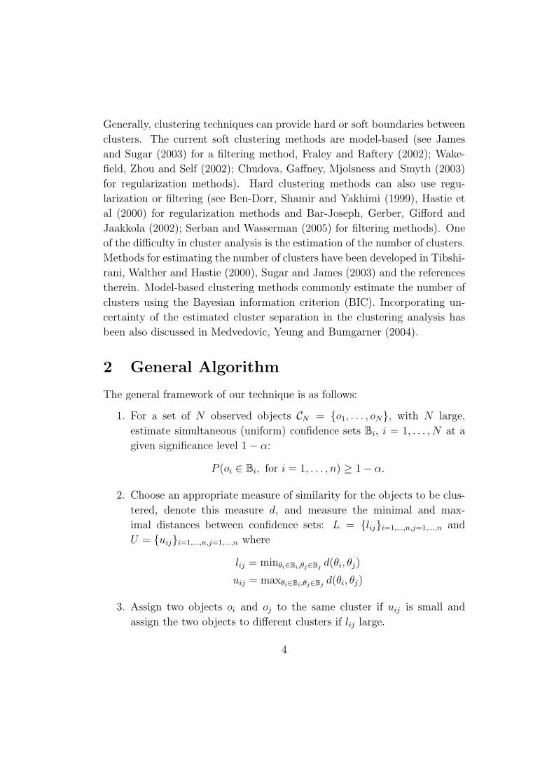
Generally, clustering techniques can provide hard or soft boundaries between

clusters. The current soft clustering methods are model-based (see James

and Sugar (2003) for a filtering method, Fraley and Raftery (2002); Wake-

field, Zhou and Self (2002); Chudova, Gaffney, Mjolsness and Smyth (2003)

for regularization methods). Hard clustering methods can also use regu-

larization or filtering (see Ben-Dorr, Shamir and Yakhimi (1999), Hastie et

al (2000) for regularization methods and Bar-Joseph, Gerber, Gifford and

Jaakkola (2002); Serban and Wasserman (2005) for filtering methods). One

of the difficulty in cluster analysis is the estimation of the number of clusters.

Methods for estimating the number of clusters have been developed in Tibshi-

rani, Walther and Hastie (2000), Sugar and James (2003) and the references

therein. Model-based clustering methods commonly estimate the number of

clusters using the Bayesian information criterion (BIC). Incorporating un-

certainty of the estimated cluster separation in the clustering analysis has

been also discussed in Medvedovic, Yeung and Bumgarner (2004).

2 General Algorithm

The general framework of our technique is as follows:

1. For a set of N observed objects CN = {o1, . . . , oN}, with N large,

estimate simultaneous (uniform) confidence sets Bi, i = 1, . . . , N at a

given significance level 1− α:

P (oi ∈ Bi, for i = 1, . . . , n) ≥ 1− α.

2. Choose an appropriate measure of similarity for the objects to be clus-

tered, denote this measure d, and measure the minimal and max-

imal distances between confidence sets: L = {lij}i=1,...,n,j=1,...,n and

U = {uij}i=1,...,n,j=1,...,n where

lij = minθi∈Bi,θj∈Bjd(θi, θj)

uij = maxθi∈Bi,θj∈Bjd(θi, θj)

3. Assign two objects oi and oj to the same cluster if uij is small and

assign the two objects to different clusters if lij large.

4

In the following section, the algorithm above is implemented for a partic-

ular type of objects, specifically, for curves.

3 Clustering Curves

The general setting is:

Yij = fi(tij) + σiεij, i = 1, . . . , N, j = 1, . . . , m (1)

where the errors εij are assumed independent with E(εij) = 0 and V ar(εij) =

1. Yij is the jth observation on the ith curve where N is typically much larger

than m. Without loss of generality, we assume that the design points tij are

in [0, 1] and fixed, but they are not necessarily equally spaced. For ease of

notation, we assume that all the curves are observed across equal number of

design points m, but this assumption can be relaxed.

3.1 Distance Definition

Our main objective is to cluster the curves fi for i = 1, . . . , N by shape

similarity. Shape similarity can be defined in terms of the similarity features

of primary interest. For example, if qualitative features such as number

of modes are of main interest, shape similarity measures shall capture the

modality of the curves. If global shape similarity is the feature of interest, a

goodness-of-fit measure will suffice. Examples of goodness-of-fit distances are

the Lp norms for p = 1, 2 . . . ,∞. To account for different variability within

each curve and to cluster regardless of scale, one can apply the Lp norm to

the standardized curves defined as:

f(x) =f(x)− ∫ 1

0f(s) ds√∫ 1

0

(f(t)− ∫ 1

0f(s) ds

)2

dt

.

The shape similarity measure for two curves f and g becomes:

ρ(f, g) = ||f − g||p =(∫ 1

0(f(x)− g(x))p

)1/p

, (2)

5

where 1− ρ(f, g) for p = 2 is the Spearman’s correlation. Other shape sim-

ilarity measures are the rank correlation as presented in Heckman and Za-

mar (2000) and the similarity measures introduced in Marron and Tsybakov

(1995). The measures in Marron and Tsybakov (1995) quantify the similarity

between two curves by measuring the distances between their graphs.

If ρ(f1, f2) is the similarity measure between two curves/objects f1 and f2

(e.g. Lp norm for standardized curves), we define the maximal and minimal

distances between the confidence sets of f1 and f2, B1 and B2, as:

MAX(B1,B2) = supf1∈B1,f2∈B2

ρ(f1, f2) and MIN(B1,B2) = inff1∈B1,f2∈B2

ρ(f1, f2).

If B1 and B2 are 1− α simultaneous confidence sets for f1 and f2, since

P (f1 ∈ B1 and f2 ∈ B2) ≥ 1− α,

the maximal and minimal measures bound the true distance between f1 and

f2 with probability 1− α:

P (MIN(B1,B2) ≤ ρ(f1, f2) ≤ MAX(B1,B2)) ≥ 1− α.

For a clustering of K clusters denoted as {C1, . . . , , CK} where each cluster

Ck contains nk objects for k = 1, . . . , K, we define the estimated within and

between clustering variabilities as below:

W (C) =∑K

k=11

n2k

∑i,j∈Ck

uij

B(C) =∑K

k=1,l=1,k 6=l1

nknl

∑i∈Ck

∑j∈Cl

lij

where lij = MIN(Bi,Bj) and uij = MAX(Bi,Bj), and the true within and

between clustering variabilities:

W (C) =∑K

k=11

n2k

∑i,j∈Ck

dij

B(C) =∑K

k=1,l=11

nknl

∑i∈Ck

∑j∈Cl

dij

where dij is the true distance between fi and fj, ρ(fi, fj). Based on the

notations above, we obtain the following lemma. The proof of this lemma is

briefly discussed in the Appendix.

6

Lemma 1 For a set of curves or objects with 1 − α simultaneous confidence

sets

P (fi ∈ Bi for i = 1, . . . , n) ≥ 1− α,

the relationship between the within and between variabilities becomes

P(

W (C) ≤ W (C) and B(C) ≤ B(C)

)≥ 1− α.

Subsequently, we will need to assign the cluster membership by minimiz-

ing the estimated within variability and maximizing the estimated between

variability as defined in this lemma.

To exemplify our general algorithm, we will consider the L2 norm applied

to standardized curves. We will show how to estimate the maximal and

minimal measures in the next section.

3.2 Distance Estimation

Let f =∑∞

r=0 θ1rψr and g =∑∞

r=0 θ2rψr be the basis decompositions for two

functions in L2, where {ψr} is an orthonormal basis in L2 with ψ0 a constant

function. Then the (function space) correlation of the two curves can be

equivalently expressed in terms of the frequency coefficients:

cor(f, g) =

∑∞r=1 θ1rθ2r√∑∞

r=1 θ21r

√∑∞r=1 θ2

2r

=< θ1, θ2 >

||θ1||||θ2||= 1−

|| θ1

||θ1|| −θ2

||θ2|| ||2

2. (3)

where θ1 = (θ11, . . .), θ2 = (θ21, . . .). The corresponding similarity distance

becomes

ρ(f, g) = 1− cor(f, g) =|| θ1

||θ1|| −θ2

||θ2|| ||2

2. (4)

The distance ρ(f, g) is not defined for f or/and g constant since these func-

tions correspond to the origin in the space where ρ is a measure between

space vectors. Constant curves form a separate cluster and therefore, we

exclude them from the further cluster analysis.

Remark: When one of the functions f or g is close to being constant,

the denominator in the definition of the distance measure provided in (3)

7

is close to zero, which will cause estimates of the distance measures to be

very unstable, and consequently, the clustering estimation becomes unstable

also. Therefore, any clustering algorithm becomes more stable when we first

remove those curves that are close to be constant. Therefore, a first step in

our cluster analysis is to remove those observed curves that correspond to

confidence sets including the origin point.

The result above applies to any decomposition based on an orthonor-

mal basis (e.g. Fourier basis, wavelet basis, spline basis, functional principal

components, etc.). Therefore, clustering based on correlation measure in the

time domain is equivalent to clustering the standardized coefficients with Eu-

clidean distance or the cosine of the angle between the vectors of coefficients

in the transform domain.

When the similarity measure between two curves is the measure in (2)

and the two curves are decomposed using an orthonormal basis, the maximal

and minimal measures between two confidence sets of two curves become:

MAX(B1,B2) = supθ1∈B1,θ2∈B2

[1− < θ1, θ2 >

||θ1||||θ2||

]= 1− inf

θ1∈B1,θ2∈B2

< θ1, θ2 >

||θ1||||θ2||

MIN(B1,B2) = infθ1∈B1,θ2∈B2

[1− < θ1, θ2 >

||θ1||||θ2||

]= 1− sup

θ1∈B1,θ2∈B2

< θ1, θ2 >

||θ1||||θ2||.

Both the minimal and the maximal measures have close form expres-

sions when the measure of similarity between two curves is the correlation or

the Euclidean distance. We derive the expressions of these measures in the

Appendix. For other shape similarity measures we can obtain approximate

maximal and minimal distances via Monte Carlo simulations.

4 Clustering Algorithm

Next we introduce a clustering algorithm that approximately maximizes the

difference between the estimated within and between variabilities.

In the clustering procedure, we first “order” the objects according to their

closest maximal distances (min−max criterion) and we call this the ’min-

max’ gap sequence. The order matters as we use it to assign the cluster mem-

8

bership. If two objects/curves fi and fj are close with respect to their max-

imal distance MAX(Bi,Bj)}, then with high probability they are close with

respect to the true distance ρ(fi, fj). Since the algorithm assigns clusters us-

ing the maximal distances, we ensure that the within variability is small with

high probability. To obtain the ordered distances, we apply the single-linkage

tree algorithm to the maximal distance matrix U = {uij = MAX(Bi,Bj)}.But any other linkage algorithm can be used to obtain this order.

Second, we separate clusters based on the minimal distances: L = {lij =

MIN(Bi,Bj)} (max−min criterion). If two objects have large minimal dis-

tance, then with high probability they are well separated with respect to the

true distance. The separation algorithm provides the estimated number of

clusters, which ensures large between variability.

The clustering algorithm is as follows:

1. Let I(j), j = 1, . . . , N are the nodes and G(j), j = 1, . . . , N represent

the links between the nodes of the ordered distances. Hartigan (1975)

calls G the gap sequence.

(a) Find two curves/objects fi and fj such that their distance is the

smallest in the distance matrix U . Assign I(1) = i and I(2) = j,

G(1) = 0 and G(2) = uI(1),I(2).

(b) For j = 3, . . . , N , find fI(j) the object in ON r {fI(1), . . . , fI(j−1)}that has the minimum distance based on the maximal distance

matrix U to any of the objects fI(1), . . . , fI(j−1). G(j) is the cor-

responding distance.

2. Once we have the distances ordered, we separate clusters as follows:

(a) For j = 1, . . . , N − 1, compute the estimated within and between

variabilities assuming {I(1), . . . , I(j)} and I(j + 1) form two dif-

ferent clusters:

W (j) =1

j2

j∑

k=1

j∑

l=1

uI(k),I(l), B(j) =2

j

j∑

k=1

lI(k),I(j+1)

9

If W (j) ≈ B(j) then put I(j+1) in the same cluster as I(1), . . . , I(j).

Continue until W (j) ¿ B(j). That is, I(j +1) is in different clus-

ter from {I(1), . . . , I(j)}.(b) For K clusters in the sequence I(1), . . . , I(j), where {I(1), . . . , I(j1)}

is the first cluster, {I(j1 + 1), . . . , I(j2)} is the second cluster, . . .,

{I(jK−1 +1), . . . , I(j)} is the K-th cluster. Assume I(j +1) forms

a (K + 1)th cluster and compute the estimated within and be-

tween variabilities between this cluster and the Kth cluster as in

part (a): W (j, K) and B(j, K). Include I(j+1) in the Kth cluster

if W (j, K) ≈ B(j, K).

In the algorithm above, the approximation threshold is data driven. A large

threshold will provide a very parsimonious clustering, whereas smaller mean-

ingless clusters will appear as the threshold decreases.

The algorithm complexity is not larger than O(N2) since both ordering

the distances using single-linkage and separating the clusters are of order

O(N2). We have close form expressions for the minimal and maximal mea-

sures when the similarity measure is the Euclidean or the correlation, but

for other similarity measures, we may need to solve complex optimization

problems and the algorithm complexity may increase of an order higher than

O(N2).

5 Confidence Set Estimation

In this section, we present an example of simultaneous confidence set esti-

mation. For this example, we assume that the curves fi belong to a Sobolev

space F ≡ Fβ(c) of unknown order β and unknown radius c:{

f(x) =∞∑

r=0

βrψr(x) :∞∑

r=0

β2r (r + 1)2β ≤ c2

}(5)

where ψ0, ψ1, ψ2, . . . is an orthonormal basis for L2. The smoothness assump-

tion can be further extended to Besov spaces and other classes of functions

depending on the basis one chooses for basis decomposition. The smoothness

assumption is also important for estimating simultaneous confidence sets for

10

the curves fi. Uniform confidence sets for Fourier basis are constructed in

Beran and Dumbgen (1998) and for wavelet basis are derived in Genovese

and Wasserman (2004). Uniform confidence bands have been proposed for

other basis of function, for example see Ruppert, Wand and Carroll (2003)

for p-spline basis. However, using the confidence bands alone does not allow

us to easily derive and compute confidence intervals on the true distances.

In time domain, the estimated confidence sets are infinite dimensional

since they are subsets of functions in the Sobolev space (5). Since we use the

estimated confidence sets to compute the maximal and minimal distances

between two curves, we reduce the dimensionality of the space and estimate

these distances in a low dimensional space. For dimensionality reduction,

we transform the curves using a basis of functions in L2 and threshold high

resolution coefficients in the transform domain. The optimal number of di-

mensions/coefficients depends on the resolution level of the true curves and

the noise structure. Further, by clustering coarse resolution curve estimates,

we allow for low uncertainty in the estimated clustering membership. On the

other hand, by clustering fine resolution curve estimates, we may discover

more patterns. Therefore, in our procedure, the number of dimensions is a

clustering tuning parameter. We can tune the clustering uncertainty using a

multi-scale approach for the number of dimensions.

5.1 Multi-scale Method

In the example introduced in this paper, we will use a Fourier basis. If our

observations are seasonal, we use the sine-cosine basis, and otherwise, we use

the cosine basis. Define the m×m matrix Ψ = {ψr(tjr)}j=1,...,m;r=0,...,m−1 and

perform a Gram-Schmidt orthogonalization on the columns of Ψ to make the

columns orthogonal. Denote the new matrix by Φ with components φrj for

r and j = 1, . . . ,m. Let θi = (θi1, . . . , θim) the frequency coefficients

θir =1

m

m∑j=1

φrjYij.

For a given number of low frequency coefficients J , the function fJi (t) =∑J

r=0 θirψr(t) is a smoothed version of the ith curve. In this context, J

11

is a smoothing parameter. When J is small, we give up high resolution

information about fi but we can estimate fJi (t) accurately. We will probably

not discover many clusters when J is small since there is not much shape

information in fJi . As we increase J we can potentially discover more shape

information leading to more refined clusters. However, we allow for higher

uncertainty in the confidence set estimation as J increases.

The multi-scale approach is to consider all values of J simultaneously

and choose the one that leads to the clustering with low uncertainty. More

precisely, we consider all the estimates fJ or 1 ≤ J ≤ Jm where Jm = o(m).

We recommend the value Jm =√

m. This leads to confidence sets for the

curves of size OP (m−1/4), which is the smallest possible in a nonparametric

sense (Li, 1989).

The confidence set for (θi1, . . . , θiJ) is somewhat simple to estimate since

θir ≈ N(θir, σ2i /m). We have that

J∑r=1

(θir − θir)2 ≈ σ2

i

mχ2

J .

Hence,

BJi =

{(θ1, . . . , θJ) :

J∑r=1

(θr − θr)2 ≤ σ2

i χ2J,α′

m

}(6)

is an approximate 1 − α′ confidence set for (θi1, . . . , θiJ). We take α′ =

α/(JmN) to ensure that the coverage is uniform over curves i and scales J .

That is,

P(

fi ∈ BJi for all i = 1, . . . , N for all J = 1, . . . , m

)' 1− α.

If one prefers a clustering method without the input of a tuning param-

eter, in the next section, we show how to find a global estimate for the

smoothing parameter and how to estimate uniform confidence sets.

5.2 Global Method

Using the global smoothing parameter as in Serban and Wasserman (2005),

we can apply the method in Beran and Dumbgen (1998) for constructing a

12

confidence set Bi for fi. Fix α > 0 and let

Bi =

{(θi1, . . . , θim) :

m∑r=1

(θir − θir)2 ≤ s2

i

}(7)

where

s2i =

z αN

τi√m

+ Ri(J), Ri(J) =Jσ2

i

m+

m∑r=J+1

(θ2

ir −σ2

i

m

)

+

,

zα is the α quantile of the standard normal and τi is given in the Appendix.

In the formulation above, Ri(J) is an estimate of the risk for fJi as provided

by Beran and Dumbgen (1998) and J is the the global smoothing parameter

as derived by Serban and Wasserman (2005). The corresponding confidence

set for fi is {∑mr=1 θirψr(x) : θ ∈ Bi}. For notational convenience, the

confidence set for fi will also be denoted by Bi.

The confidence sets are asymptotically uniform over the Sobolev space

and uniform over curves. But the uniformity over both the Sobolev space and

over curves will result in large confidence sets. We cannot relax the uniformity

over curves since we observe the curves simultaneously. But we can relax the

uniformity over the Sobolev space using the multi-scale approach discussed

in Section 5.1.

Based on the theorems in Beran and Dumbgen (1998), we obtain the

following result:

Theorem 1 Let Fβ(c) denote a Sobolev space of order β and radius c. Then,

for any β > 1/2 and any c > 0,

lim infN→∞

supf1,...,fN∈Fβ(c)

P(

MIN(Bi,Bj) ≤ d(fi, fj) ≤ MAX(Bi,Bj), ∀i, j = 1, . . . , N

)≥ 1− α.

Thus we estimate the distance between two curves with a simultaneous (1−α)

confidence interval given by the minimal and maximal distances between their

confidence sets.

The proof of this result derives from Theorem 1 in Serban and Wasserman

(2005), which states that

lim infN→∞

supf1,...,fN∈Fβ(c)

P(

fi ∈ Bi, ∀i = 1, . . . , N

)≥ 1− α

13

under the conditions in theorem 1 of this paper.

As already mentioned in Section 1, we can derive an inequality of the

within and between variabilities under the conditions stated in Theorem 1.

Lemma 2 states that these inequalities hold with high probability asymptot-

ically.

Lemma 2 Let C be a clustering of K clusters: {C1, . . . , , CK}. Similar to the

result in Lemma 1 and under the conditions of Theorem 1,

lim infN→∞

supf1,...,fN∈Fβ(c)

P(

W (C) ≤ W (C) and B(C) ≤ B(C)

)≥ 1− α.

The proof of this lemma follows directly from Theorem 1 and the proof

is similar to lemma 1 presented in the Appendix.

Similar results can be derived for the multi-scale approach.

6 Method Evaluation: Synthetic Example

We evaluate our clustering technique using synthetic data. The synthetic

example consists of 4 different patterns according to the regression model (1)

with m = 25, N = 500 and σi ∈ [.5, 1.5]. The synthetic data are generated

from the model below

Yij = µi + Fk(tj) + Nm(0, σi), i = 1, . . . , 500, j = 1, . . . , 25, k = 1, 2, 3, 4

where µi ∈ [1, 5], and Fk for k = 1, 2, 3, 4 are four different patterns. The

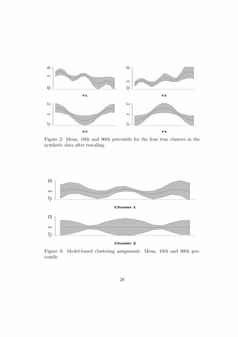
mean, 90th and 10th percentiles of the data in the four clusters are in Figure

2. We generate 50 curves from the first pattern (upper plot, left), 100 from

the second pattern (upper plot, right), 150 from the third pattern (lower

plot, left), and 200 from the fourth pattern.

6.1 Clustering Error Rate

We compare the performance of different clustering techniques using a mea-

sure for clustering error as described below.

14

Let Tn,K and Tn,K denote the true clustering map and, respectively, the

estimated clustering map:

Tn,K(f, g) =

{1 if f and g are in the same cluster0 otherwise

(8)

The two clustering maps depend on the number of clusters.

The clustering error rate for K clusters is

η(K) =1(N2

)∑r<s

I

(Tn,K(fr, fs) 6= Tn,K(fr, fs)

)(9)

This clustering error rate can also be expressed as

η = 1−R(T, T )

where R is the Rand index (Rand, 1971).

6.2 Other Methods

We will consider in this section the performance of three different clustering

algorithms. They are the model-based clustering (’mclust’ R library) intro-

duced in Yeung et al (2001), the filtering clustering technique introduced by

Bar-Joseph et al (2001), and hierarchical clustering of the estimated curves.

Last, we describe the performance of the method introduced in this paper.

Yeung et al (2001). The model-based clustering technique introduced in

this paper estimates the number of clusters using the BIC approximation

criterion. We apply this technique to the synthetic data presented above.

The method assigns the four groups of curves to two clusters with the means,

10th and 90th percentiles presented in Figure 3. The clustering error is about

.25.

Bar-Joseph et al (2001). The clustering strategy introduced by Bar-Joseph

and colleagues is a filtering method that provides hard clustering member-

ship. We apply this technique to the synthetic data presented above. This

method captures the main patterns in the synthetic data when fixing the

number of clusters to the true number of patterns. Therefore, the method

requires the input of the number of clusters. The clustering error is about

15

.09 before removing the unstable curves as defined in Section 3.2, and about

.03 after removing these curves.

Hierarchical clustering. We apply the single-linkage clustering to the es-

timated curves. The clustering error is about .15. After discarding the

confidence sets including the origin, the hierarchical clustering algorithm as-

signs the cluster membership correctly. Similar to the method introduced

in Bar-Joseph et al (2001), for hierarchical clustering, we need to input the

number of clusters.

Clustering Confidence Sets. In Figure 4, we present the gap sequence of

the single-linkage tree based on the distance point estimates for our synthetic

example. In Figure 5, we present the gap sequence for the single-linkage tree

based on the maximal (upper bound) distances as provided by our method.

In contrast to the point estimation based clustering, we clearly separate the

four clusters when using the lower and upper distance bounds. Subsequently,

using our algorithm, we estimate four clusters and the algorithm assigns the

cluster membership errorless.

For all the methods compared in this paper, the clustering membership

is more stable after removing the synthetic curves with low signal-to-noise

ratio which result in large confidence sets containing the origin.

7 Example: Q-ratio Evaluation in Manufac-

turing Sector

The individual performance of a firm’s business or operation is indicated

by its financial status revealed in its financial statements such as balance

sheets, income statements, statements of cash flows, and retained earning

statements. Comparing companies within an industry sector requires ad-

justing the accounting information for size differences between firms. Subse-

quently, it is unreasonable to use raw items from financial statements when

performing a comparative study across multiple companies.

There are two ways to remove size effects. The first is to express each

item on the financial statement as a percentage of one representative item,

which is called a common-size statement. The second method to evaluate

16

the current financial condition and performance of firms is to compute ratios

from financial statements. In this paper, we use a market value ratio called

Q-ratio to indicate the true worth of a firm’s assets in the market. Ross,

Westerfield, and Jaffe (2005) explain that Tobins Q ratio divides the market

value of all of the firm’s debt plus equity by the replacement value of the firm’s

assets. This ratio was derived by James Tobin, Nobel laureate in Economics.

A Q-ratio between 0 and 1 indicates that the value of a firm’s stock is not

enough to replace its assets. This suggests overvaluation of the stock. When

the Q-ratio is larger than 1, the stock is undervalued. In Tobin’s model, this

method of stock valuation guides investment decisions (Investopedia, 2006).

We apply our clustering method to companies listed in the Compustat

Global database in manufacturing sectors categorized using NAICS - North

American Industry Classification System. The U.S., Canada, and Mexico,

members of NAFTA, developed NAICS to provide statistical comparability

of firm’s operational activity across North America. (U.S. Census Bureau

2006). Table 1 shows the NAICS code and corresponding sector names of

the companies studied in this paper. We investigate the annual financial

statements starting with 1990 to 2005. Also we only consider the set of

companies with none or a few missing/incomplete data values. The total

number of companies is about 850.

We derived the Q-ratio from financial statements included in Compustat

database and adjusted for long-term economic changes as provided by a re-

search group located in Chicago (Ativo Research, Llc). The adjustments are

documented in Madden (1999).

We apply the procedure presented in this paper to the Q-ratio patterns,

and for J = 3, there are about 200 companies out of about 850 that have

Q-ratios changing considerably over the past 16 years as their estimates con-

fidence sets are away from origin. For the 200 time-varying patterns, we

identify four well separated clusters with smaller sub-clusters as shown in

Figure 6. The patterns within each cluster are presented in Figure 7. The

largest cluster consists of curves with lower changes in Q-ratio values over

time. However, most of the companies in cluster one to three are under-

valued at different times over the 16 years: at the beginning of 1990 for

companies in cluster 1, during the internet economic burst for companies in

17

cluster 2, and close to the macro-economic crisis in 2000 for companies in

cluster 3. Examples of companies in each of the four clusters are listed in

the Appendix.

Figure 8 shows the smoothed patterns as identified with the method in

Bar-Joseph et al (2001) for four clusters. As provided in this figure, the four

clusters contain mixed patterns.

8 Discussion

In this article, we have presented a novel approach to clustering a large

number of observed curves but the general strategy can be applied to other

types of objects. The novelty of our technique consists of clustering based on

the maximal and minimal distances between confidence sets. Consequently,

we obtain confidence interval estimates for the distances between curves. The

upper limits of these confidence intervals are used to assign curves in the same

cluster, and the lower bounds are used to assign curves in different clusters,

which in turn will also give the estimated number of clusters. We used

the single-linkage tree to assign the cluster membership, but other clustering

algorithms can be used (e.g. the minimum spanning tree or k-ary clustering).

Removing curves/objects with confidence sets containing the origin, we

obtain a more stable clustering. As we increase the smoothing parameter, the

radius of the confidence sets increases also, and therefore, more confidence

sets will contain the origin. In our synthetic example, for J = 2, about 36

out of 500 confidence sets contain the origin. For J = 5, the number of

confidence sets containing the origin increases to 80. On the other hand, at

higher uncertainty or less smoothing, we expect to discover more patterns.

Consequently, we will choose a low uncertainty level or small smoothing

parameter for which we detect all or most of the patterns discovered at

finer resolution. In our synthetic example, we discover four patterns, for all

smoothing levels from J = 2 to J = 5, and the separation between the four

clusters is similar across all these smoothing levels. See Figure 5. Therefore,

J = 2 will be low enough to identify the clustering structure in the data.

One other advantage of using our approach is that we can establish a

better separation between clusters. Figure 4 displays the gap sequence of

18

the clustering assignment based on the point distance estimates using single-

linkage tree algorithm. Figure 5 displays the gap sequence of the clustering

assignment based on the maximal distances U = {uij} using single-linkage

algorithm for different smoothing parameters. In the same figure, we include

the lower bound of the gap sequence. There is a clearer cluster separation

in the gap sequence based on the upper and lower bounds of the distances

(Figure 5) than in the gap sequence based on the point distance estimates

(Figure 4).

Last, in our empirical example, the gap sequence divides in smaller sub-

clusters at higher resolution level. On the other hand, at lower smoothing

parameter J , the large clusters are well separated without being divided

in many sub-clusters. Therefore, our method gives the flexibility to choose

between a finer or coarser clustering structure by changing the resolution

level.

There are a few different research directions to take from here. One

challenge is to design a clustering algorithm that uses the information of the

upper and lower limits simultaneously. Another challenge is to extend the

main strategy to clustering algorithms that do not use the distance matrix

information only (e.g. k-means).

Appendix

Computing the maximal and minimal distances

In this section we compute the maximal distance when the similarity measure

between two objects is the Euclidean distance or the correlation coefficient.

Under Euclidean distance, the maximal and minimal distances between two

confidence sets are:

MAXE(B1,B2) = supθ1∈B1,θ2∈B2

||θ1 − θ2||2

MINE(B1,B2) = infθ1∈B1,θ2∈B2

||θ1 − θ2||2.

19

Under the correlation measure, the maximal and minimal distances between

two sets are:

MAXC(B1,B2) = supθ1∈B1,θ2∈B2

(1− < θ1, θ2 >

||θ1||||θ2||)

MINC(B1,B2) = infθ1∈B1,θ2∈B2

(1− < θ1, θ2 >

||θ1||||θ2||)

Solution for the Euclidean distance.

When the Euclidean distance is the measure between two objects, the

two distances are rather easy to compute:

MAXE(B1,B2) = ||C1 − C2||+ (r1 + r2)

MINE(B1,B2) = (||C1 − C2|| − (r1 + r2)) I (||C1 − C2|| − (r1 + r2) >= 0)

where r1 and r2 are the radius for ball B1 and, respectively, for ball B2, and

||C1 − C2|| is the Euclidean distance between the centers of the confidence

sets. I() denotes the indicator function.

Solution for the correlation distance.

We assume that the smoothing parameter is J and thus only the first J

coefficients of θ are non-zero. Thus in the J dimensional space

< θ1, θ2 >

||θ1||||θ2||= cos

(∠

(θ1, θ2

)).

The problem reduces to finding the maximum (for MAXC) and the minimum

(for MINC) angle between any two points in the confidence sets B1 and

B2. The relationship between the maximum and minimum angles with the

maximal and minimal distances are derived below

MAX(B1,B2) = 1− infθ1∈B1,θ2∈B2

< θ1, θ2 >

||θ1||||θ2||= 1− cos

(sup

θ1∈B1,θ2∈B2

∠(θ1, θ2

))

MIN(B1,B2) = 1− supθ1∈B1,θ2∈B2

< θ1, θ2 >

||θ1||||θ2||= 1− cos

(inf

θ1∈B1,θ2∈B2

∠(θ1, θ2

)).

20

The centers of the two confidence sets are C1 and C2, and the origin of

the J dimensional space is O. The tangents from the origin to the confidence

sets intersect the balls in T1 and T2. We want to find the maximum and the

minimum angle ˆT1OT2. See Figure 9.

Denote the coordinates of T1, T2, C1, C2 and O:

t1 = (t11, . . . , t1J) , t2 = (t21, . . . , t2J)

c1 = (c11, . . . , c1J) , c2 = (c21, . . . , c2J)

o = (o1, . . . , oJ).

We want to optimize the function:

f(t1, t2) =< t1, t2 >

||t1||||t2|| =

∑Jj=1 t1jt2j√∑J

j=1 t21j

∑Jj=1 t22j

over the set (t1, t2) ∈ B1 ×B2 where

Bi = {ti = (ti1, . . . , tiJ) :J∑

j=1

t2ij =J∑

j=1

c2ij−r2

i (1) andJ∑

j=1

(tij − cij)2 = r2

i (2)} =

{ti = (ti1, . . . , tiJ) : ||ti||2 = ||ci||2 − r2i and ||ti − ci|| = r2

i }where the first condition is due to the tangent from the origin to the confi-

dence ellipsoids and the second condition is that T1 and T2 are on the envelope

of the two ellipsoids.

The equivalent optimization problem is to minimize/maximize:

J∑j=1

t1jt2j =< t1, t2 >

with t1 ∈ B1 and t2 ∈ B2.

We solve this optimization problem using Lagrange multipliers. The ob-

jective function is:

f(t1, t2) =< t1, t2 >

with the constraints

gi(t1, t2) =< ti, ci > −(||ci||2 − r2i )

21

hi(t1, t2) = ||ti||2 − ((||ci||2 − r2i )

Denote ||ci||2 − r2i = s2

i for the ease of notation.

The optimization problem by Lagrange’s theorem is equivalent to solving:

∆f(t1, t2) = µ1∆g1(t1, t2)+µ2∆g2(t1, t2)+λ1∆h1(t1, t2)+λ2∆h2(t1, t2) (10)

with the first order derivatives

∆f(t1, t2) = (t21, . . . , t2J , t11, . . . , t1J)

∆g1(t1, t2) = (c11, . . . , c1J , 0, . . . , 0)

∆g2(t1, t2) = (0, . . . , 0, c21, . . . , c2J)

∆h1(t1, t2) = (2t11, . . . , 2t1J , 0, . . . , 0)

∆h2(t1, t2) = (0, . . . , 0, 2t21, . . . , 2t2J).

We translate the equation 10 into a 2J + 4 equations with 2J + 4 unknowns.

For j = 1, . . . , J , {t1j = 2λ2t2j + µ2c2j

t2j = 2λ1t1j + 2µ1c1j(11)

with the solution: {t1j =

c2jµ2+2c1jλ2µ1

1−4λ1λ2

t2j =c1jµ1+2c2jλ1µ2

1−4λ1λ2.

(12)

Thus we have to find only λ1, λ2, µ1, and µ2 by using the constrains

gi(t1, t2) = 0, hi(t1, t2) = 0.

which can be translated into 4 equations with 4 unknowns:

µ2<c1,c2>+2λ2µ1||c1||21−4λ1λ2

= s21

µ1<c2,c1>+2λ1µ2||c2||21−4λ1λ2

= s22

µ22||c2||2+4λ2

2µ21||c1||2+4λ2µ1µ2<c1,c2>

(1−4λ1λ2)2= s2

1µ2

1||c1||2+4λ21µ2

2||c2||2+4λ1µ1µ2<c1,c2>

(1−4λ1λ2)2= s2

2.

(13)

This last system of equations can be solved using Mathematica. The system

will have more than one solution. We take the solution which minimizes (for

MAXC) and maximizes (for MINC) < t1, t2 >.

22

Proof of Lemma 1

The result is derived from the following inequality:

P

(fi ∈ Bi, fj ∈ Bj, i, j = 1, . . . , N

)≤

P(

MIN(Bi,Bj) ≤ d(fi, fj) ≤ MAX(Bi,Bj), i, j = 1, . . . , N

).

Therefore, if Bi for i = 1, . . . , N are 1 − α simultaneous confidence sets for

the set of N curves, then

P(

MIN(Bi,Bj) ≤ d(fi, fj) ≤ MAX(Bi,Bj), i, j = 1, . . . , N

)≥ 1− α.

From the definition of uij and lij distances, the inequality above can be re-

expressed as:

P(

ρ(fi, fj) ≤ uij and ρ(fi, fj) ≥ lij i, j = 1, . . . , N

)≥ 1− α

Since ρ(fi, fj) ≤ uij for all i, j = 1, . . . , N implies that W (C) ≤ W (C) and

ρ(fi, fj) ≥ lij for all i, j = 1, . . . , N implies that B(C) ≥ B(C), together with

the inequality above we have the result in this lemma.

τ 2 estimation

For the high component variance estimator σ2i for curve fi

σi2 =

1

m− L

m∑i=L+1

θ2ij.

we estimate

τ 2i =

m∑j=1

(1 +

1− 2cj

m− J

)(4(θ2

ij − σ2)+σ2 + 2σ4) + 4σ2

k∑j=1

2cj

m− J(θ2

ij − σ2)+

where cj is 1 for j ≥ J + 1 and 0 otherwise.

The estimated variance of τ 2 is derived in Serban and Wasserman (2005).

23

Companies names by clusters

Below I included samples of companies and their cluster memberships.

Cluster 1:

Healthcare Technologies Ltd, Cooper Tire & Rubber Co, Ap Pharma Inc,

Lancer Orthodontics Inc, Phazar Corp.

Cluster 2:

3Com Corp, Topps Co Inc, Mgp Ingredients Inc Scientific, Technologies

Inc, Spectrum Signal Processing, Aleris International Inc.

Cluster 3:

Pfizer Inc, Medtronic Inc, Biogen Idec Inc, Bristol-Myers Squibb Co,

Nanometrics Inc, Lilly (Eli) & Co, Colgate-Palmolive Co.

Cluster 4:

Allergan Inc, Avon Products, Varian Medical Systems Inc, Alcoa Inc,

Novo-Nordisk A/S -Adr, Protein Design Labs Inc, Tektronix Inc, Procter &

Gamble Co, Amylin Pharmaceuticals Inc, Wireless Telecom Group Inc, Lipid

Sciences Inc, Texas Instruments Inc.

References

[1] Ziv Bar-Joseph, Erik D. Demaine, David K. Gifford, Angle M. Hamel,

Tommi S. Jaakkola and Nathan Srebro, “K-ary Clustering with Opti-

mal Leaf Ordering for Gene Expression Data”,Proceedings of the 2nd

Workshop on Algorithms in Bioinformatics (WABI 2002) LNCS 2452,

pp 506-520.

[2] Bar-Joseph, Z., Gerber, G., Gifford, D.K., Jaakkola, T.S. (2002). “A new

approach to analyzing gene expression time series data”, Proceedings of

the 6th Annual International Conference on RECOMB, pp 39-48.

24

[3] Ben-Dorr, A, Shamir, R. and Yakhimi, Z. (1999). “Clustering gene ex-

pression patterns”, J. of Computational Biology.

[4] Beran, R., Dumbgen, L. (1998), “Modulation of estimators and confi-

dence sets”, Annals of Statistics, 26, 5, pp 1826-1856.

[5] Chudova, D., Gaffney, S., Mjolsness, E., Smyth, P.(2003), ”Translation-

invariant mixture models for curve clustering”,Proceedings of the ninth

ACM SIGKDD international conference on Knowledge discovery and

data mining, 79 - 88.

[6] Fraley, C., Raftery, E. (2002), ”Model-Based Clustering, Discriminant

Analysis, and Density Estimation”, Journal of the American Statistical

Association, 97, 611-631.

[7] Genovese, C., Wasserman, L. (2005), “Confidence sets for nonparametric

wavelet regression”, The Annals of Statistics, Volume 33, Number 2,

698-729.

[8] Hartigan, J.A. (1975), Clustering Algorithms, John Wiley & Sons, Inc.

[9] Hastie, T., Tibshirani, R., Eisen, M., Alizadeh, A., Levy, R., Staudt, L.,

Chan, W., Botstein, D., Brown, P. (2000), ”’Gene shaving’ as a method

for identifying distinct sets of genes with similar expression patterns”,

Genome Biology, I(2):research0003.1-0003.21.

[10] Heckman, N., Zamar, R. (2000), “Comparing the shapes of regression

functions”, Biometrika, 87, 135-144.

[11] James, G.M., Sugar,C.A. (2003), “Clustering for sparsely sampled func-

tional data”, Journal of the American Statistical Association, 98, p397.

[12] Li, Ker-Chau (1989), “Honest confidence regions for nonparametric re-

gression”, Annals of Statistics, 3, pp 1001-1008.

[13] Marron, J.S., Tsybakov, A.B. (1995), “Visual Error Criteria for Quali-

tative Smoothing”, Journal of the American Statistical Association, 90,

499-507.

25

[14] Madden B. J. (1999), “CFRoI Valuation - A Total System Approach to

Valuing the Firm”, 1st ed., Buttterworth-Heinemann, Oxford.

[15] Medvedovic, M., Yeung, K.Y., Bumgarner, R. (2004), “Bayesian mix-

ture model based clustering of replicated microarray data”, Bioinfor-

matics, 20,1222-1232.

[16] Rand, W. M. (1971), “Objective criteria for the evaluation of clustering

methods”.Journal of the American Statistical Association , 66, pp. 846-

850.

[17] Ruppert, D., Wand, M.P., Carroll, R.J. (2003), Semiparametric Regres-

sion, Cambridge University Press.

[18] Serban, N., Wasserman, L. (2005), “CATS: Cluster after transformation

and smoothing”, Journal of the American Statistical Association, 100,

990-999.

[19] Tibshirani, R., Walther, G., Hastie, T. (2001), “Estimating the number

of clusters in a dataset via the Gap statistic”, Journal of the Royal

Statistical Society, B, 63, 411-423.

[20] Yeung, K.Y., Murua, A., Raftery, A., Ruzzo, W.L. (2001). “Model-

Based Clustering and Data Transformations for Gene Expression Data”,

Bioinformatics, 17, 977-987.

[21] Wakefield, J., Zhou, C., Self, S. (2002), ”Modelling Gene Expression

Data over Time: Curve Clustering with Informative Prior Distribu-

tions”, Bayesian Statistics 7, Proceedings of the Seventh Valencia In-

ternational Meeting, 2003.

[22] Ross, S.A., Westerfield, R.W. and Jaffe, J.F. (2005), “Corporate Fi-

nance”, 7th ed. McGraw-Hill, New York

[23] Sugar, C., and James, G. (2003), ”Finding the Number of Clusters in a

Data Set : An Information Theoretic Approach”, Journal of the Amer-

ican Statistical Association, 98, 750-763.

26

−1.5 −1.0 −0.5 0.0 0.5 1.0

−0.

50.

00.

51.

0

Figure 1: 2-dimensional estimated confidence sets for seven observations sim-ulated from two similar patterns but with different variability levels and atdifferent scales.

[24] Tibshirani, R., Walther, G., Hastie, T. (Dec 2000), “Estimating the

number of clusters in a dataset via the Gap statistic”. Technical report,

published in Journal of the Royal Statistical Society, B,2000.

27

−23

015

F1

−12

023

F2

−17

017

F3−1

70

17F4

Figure 2: Mean, 10th and 90th percentile for the four true clusters in thesynthetic data after rescaling.

−17

023

Cluster 1

−17

023

Cluster 2

Figure 3: Model-based clustering assignment: Mean, 10th and 90th per-centile.

28

31 Manufacturing

321 Wood Product Manufacturing322 Paper Manufacturing323 Printing and Related Support Activities324 Petroleum and Coal Products Manufacturing325 Chemical Manufacturing326 Plastics and Rubber Products Manufacturing327 Nonmetallic Mineral Product Manufacturing331 Primary Metal Manufacturing332 Fabricated Metal Product Manufacturing333 Machinery Manufacturing334 Computer and Electronic Product Manufacturing335 Electrical Equipment, Appliance, and Component Manufacturing336 Transportation Equipment Manufacturing337 Furniture and Related Product Manufacturing339 Miscellaneous Manufacturing

Table 1: Manufacturing Industries in 32 and 33 NAICS listings.

0.0

0.6

1.2

Gap sequence

Figure 4: Gap sequence of the single-linkage tree of the point distance esti-mates.

29

0 100 200 300 400

0.0

0.4

0.8

1.2

Gap sequence for J=2

0 100 200 300 4000.0

0.4

0.8

1.2

Gap sequence for J=3

0 100 200 300 400

0.0

0.4

0.8

1.2

Gap sequence for J=4

0 100 200 300 400

0.0

0.4

0.8

1.2

Gap sequence for J=5

Figure 5: Gap sequence of the maximal distances (shown in black) and thecorresponding minimal distances (shown in blue) for different smoothing lev-els.

30

0.00.5

1.01.5

Gap s

eque

nce

Cluster 1 Cluster 2 Cluster 3 Cluster 4

Figure 6: Gap sequence of the maximal distances (shown in black) andthe corresponding minimal distances (shown in blue) with cluster separa-tion thresholds shown in brown.

1990 1995 2000 2005

05

1015

year

Smoo

thed Q

−ratio

patte

rn

cluster 1

1990 1995 2000 2005

05

1015

year

Smoo

thed Q

−ratio

patte

rn

cluster 2

1990 1995 2000 2005

05

1015

year

Smoo

thed Q

−ratio

patte

rn

cluster 3

1990 1995 2000 2005

05

1015

year

Smoo

thed Q

−ratio

patte

rn

cluster 4

Figure 7: Clustering patterns as identified by clustering maximal and mini-mal distance.

31

1990 1995 2000 2005

05

1015

year

Smoo

thed Q

−ratio

patte

rn

cluster 1

1990 1995 2000 2005

05

1015

year

Smoo

thed Q

−ratio

patte

rn

cluster 2

1990 1995 2000 2005

05

1015

year

Smoo

thed Q

−ratio

patte

rn

cluster 3

1990 1995 2000 20050

510

15year

Smoo

thed Q

−ratio

patte

rn

cluster 4

Figure 8: Clustering patterns as identified by the Bar Joseph et al (2001)method.

angle

Minangle

Max

Figure 9: 2-dimensional example for maximum and minimum angle: Com-puting the maximal and minimal distances under correlation measure.

32