OLAP and Data Warehousingvizclass/classes/infsci2711_s2w/data/olap_and_dw... · A modern data...
21
OLAP and Data Warehousing Advanced Topics in Database Management (INFSCI 2711) Some materials are from INFSCI2710’a Database Management Systems, R. Ramakrishnan and J. Gehrke and from https://www.kimballgroup.com/ Vladimir Zadorozhny, DINS, University of Pittsburgh
Transcript of OLAP and Data Warehousingvizclass/classes/infsci2711_s2w/data/olap_and_dw... · A modern data...

OLAP and Data Warehousing
Advanced Topics in Database Management (INFSCI 2711)
Some materials are from INFSCI2710’a Database Management Systems,
R. Ramakrishnan and J. Gehrke
and from
https://www.kimballgroup.com/
Vladimir Zadorozhny, DINS, University of Pittsburgh
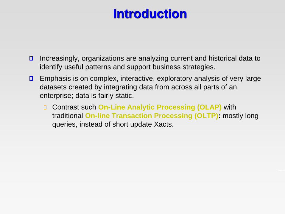
Introduction
Increasingly, organizations are analyzing current and historical data to
identify useful patterns and support business strategies.
Emphasis is on complex, interactive, exploratory analysis of very large
datasets created by integrating data from across all parts of an
enterprise; data is fairly static.
Contrast such On-Line Analytic Processing (OLAP) with
traditional On-line Transaction Processing (OLTP): mostly long
queries, instead of short update Xacts.

Three Complementary Trends
Data Warehousing: Consolidate data from many sources in one large repository.
Loading, periodic synchronization of replicas.
Semantic integration.
OLAP:
Complex SQL queries and views.
Queries based on spreadsheet-style operations and “multidimensional”view of data.
Interactive and “online” queries.
Data Mining: Exploratory search for interesting trends and anomalies (not considered in this class)
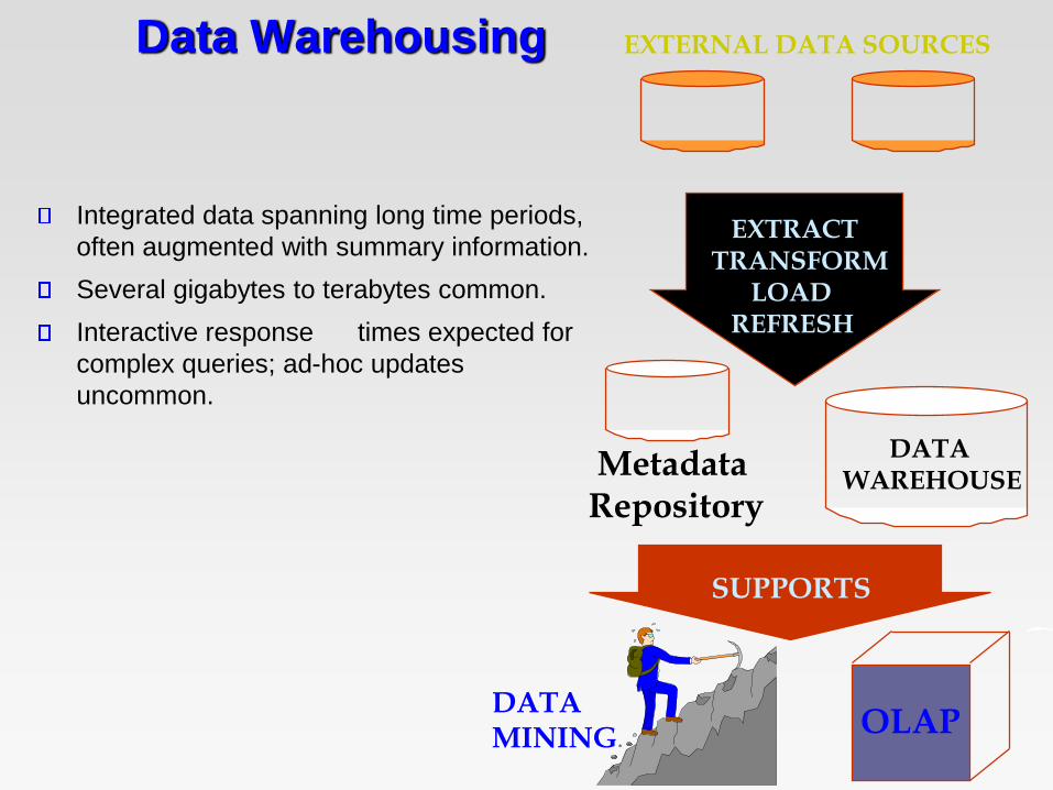
Data Warehousing
Integrated data spanning long time periods,
often augmented with summary information.
Several gigabytes to terabytes common.
Interactive response times expected for
complex queries; ad-hoc updates
uncommon.
EXTERNAL DATA SOURCES
EXTRACTTRANSFORM
LOADREFRESH
DATAWAREHOUSE
MetadataRepository
SUPPORTS
OLAPDATAMINING
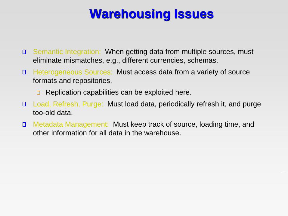
Warehousing Issues
Semantic Integration: When getting data from multiple sources, must
eliminate mismatches, e.g., different currencies, schemas.
Heterogeneous Sources: Must access data from a variety of source
formats and repositories.
Replication capabilities can be exploited here.
Load, Refresh, Purge: Must load data, periodically refresh it, and purge
too-old data.
Metadata Management: Must keep track of source, loading time, and
other information for all data in the warehouse.

Multidimensional Data
Model
Collection of numeric measures, which depend on a set of
dimensions.
E.g., measure Sales, dimensions Product (key: pid),
Location (locid), and Time (timeid).
8 10 10
30 20 50
25 8 15
1 2 3timeid
pid
11
12
13
11 1 1 25
11 2 1 8
11 3 1 15
12 1 1 30
12 2 1 20
12 3 1 50
13 1 1 8
13 2 1 10
13 3 1 10
11 1 2 35
pid
tim
eid
loci
d
sale
s
locid
Slice locid=1is shown:

MOLAP vs ROLAP
Multidimensional data can be stored physically in a (disk-resident,
persistent) array; called MOLAP systems. Alternatively, can store as a
relation; called ROLAP systems.
The main relation, which relates dimensions to a measure, is called the
fact table. Each dimension can have additional attributes and an
associated dimension table.
E.g., Products(pid, pname, category, price)
Fact tables are much larger than dimensional tables.

Dimension Hierarchies
For each dimension, the set of values can be organized in a hierarchy:
PRODUCT TIME LOCATION
category week month state
pname date city
year
quarter country
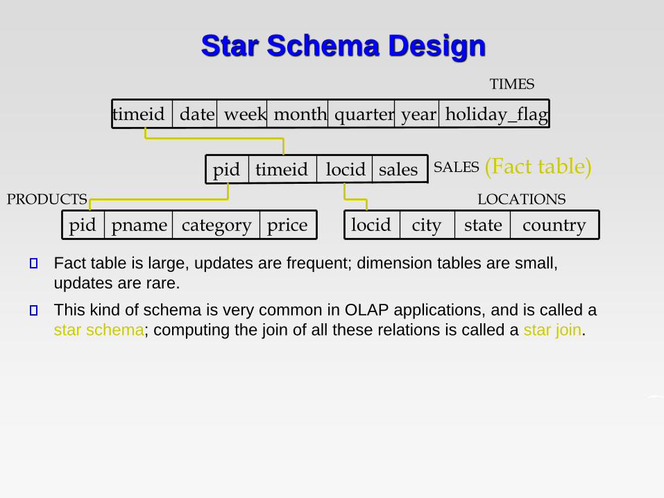
Star Schema Design
Fact table is large, updates are frequent; dimension tables are small,
updates are rare.
This kind of schema is very common in OLAP applications, and is called a
star schema; computing the join of all these relations is called a star join.
pricecategorypnamepid countrystatecitylocid
saleslocidtimeidpid
holiday_flagweekdatetimeid month quarter year
(Fact table)SALES
TIMES
PRODUCTS LOCATIONS
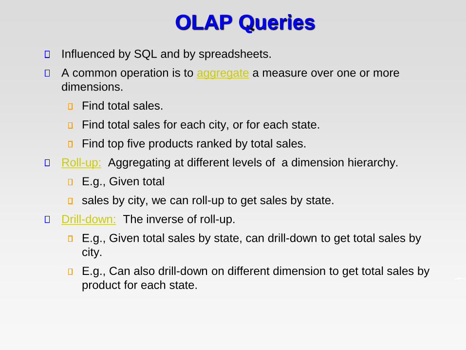
OLAP Queries
Influenced by SQL and by spreadsheets.
A common operation is to aggregate a measure over one or more
dimensions.
Find total sales.
Find total sales for each city, or for each state.
Find top five products ranked by total sales.
Roll-up: Aggregating at different levels of a dimension hierarchy.
E.g., Given total
sales by city, we can roll-up to get sales by state.
Drill-down: The inverse of roll-up.
E.g., Given total sales by state, can drill-down to get total sales by
city.
E.g., Can also drill-down on different dimension to get total sales by
product for each state.

More on Drilling Down
Drilling down means adding a row header (a grouping column) to an
existing SELECT statement.
E.g., if you’re analyzing the sales of products at a manufacturer level, the select
list of the query reads SELECT MANUFACTURER, SUM(SALES).
If you wish to drill down on the list of manufacturers to show the brands sold,
you add the BRAND row header: SELECT MANUFACTURER, BRAND,
SUM(SALES).
the GROUP BY clause in the second query reads GROUP BY
MANUFACTURER, BRAND. Row headers and grouping columns are the same
thing.
Now each manufacturer row expands into multiple rows listing all the brands
sold.
This example is particularly simple because in a star schema, both the
manufacturer attribute and the brand attribute exist in the same product
dimension table.
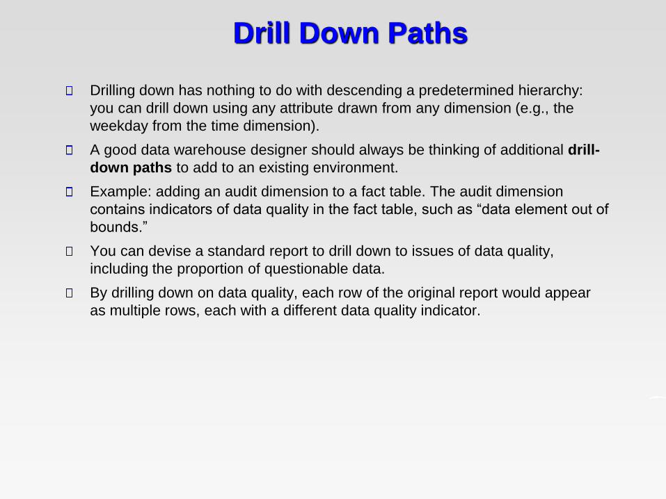
Drill Down Paths
Drilling down has nothing to do with descending a predetermined hierarchy:
you can drill down using any attribute drawn from any dimension (e.g., the
weekday from the time dimension).
A good data warehouse designer should always be thinking of additional drill-
down paths to add to an existing environment.
Example: adding an audit dimension to a fact table. The audit dimension
contains indicators of data quality in the fact table, such as “data element out of
bounds.”
You can devise a standard report to drill down to issues of data quality,
including the proportion of questionable data.
By drilling down on data quality, each row of the original report would appear
as multiple rows, each with a different data quality indicator.

Aggregate Navigator
The data warehouse must support drilling down at the user interface level with
the most atomic data possible because the most atomic data is the most
dimensional.
The atomic data must be in the same schema format as any aggregated form
of the data.
An aggregated fact table (materialized view) is a mechanically derived table of
summary records.
Aggregated fact tables (materialized views) offer immense performance
advantages compared to using the large, atomic fact tables. But you get this
performance boost only when the user asks for an aggregated result.
A modern data warehouse environment uses a query-rewrite facility called an
aggregate navigator to choose a prebuilt aggregate table whenever possible.
Each time the end user asks for a new drill-down path, the aggregate navigator
decides in real time which aggregate fact table will support the query most
efficiently.
Whenever the user asks for a sufficiently precise and unexpected drill down,
the aggregate navigator gracefully defaults to the atomic data layer.

OLAP Queries
Pivoting: Aggregation on selected dimensions.
E.g., Pivoting on Location and Time yields this cross-tabulation:
63 81 144
38 107 145
75 35 110
WI CA Total
1995
1996
1997
176 223 339Total
Slicing and Dicing: Equalityand range selections on oneor more dimensions.

Using SQL for Pivoting
The cross-tabulation obtained by pivoting can also be computed using a
collection of SQLqueries:
SELECT SUM(S.sales)FROM Sales S, Times T, Locations LWHERE S.timeid=T.timeid AND S.timeid=L.timeidGROUP BY T.year, L.state
SELECT SUM(S.sales)FROM Sales S, Times TWHERE S.timeid=T.timeidGROUP BY T.year
SELECT SUM(S.sales)FROM Sales S, Location LWHERE S.timeid=L.timeidGROUP BY L.state
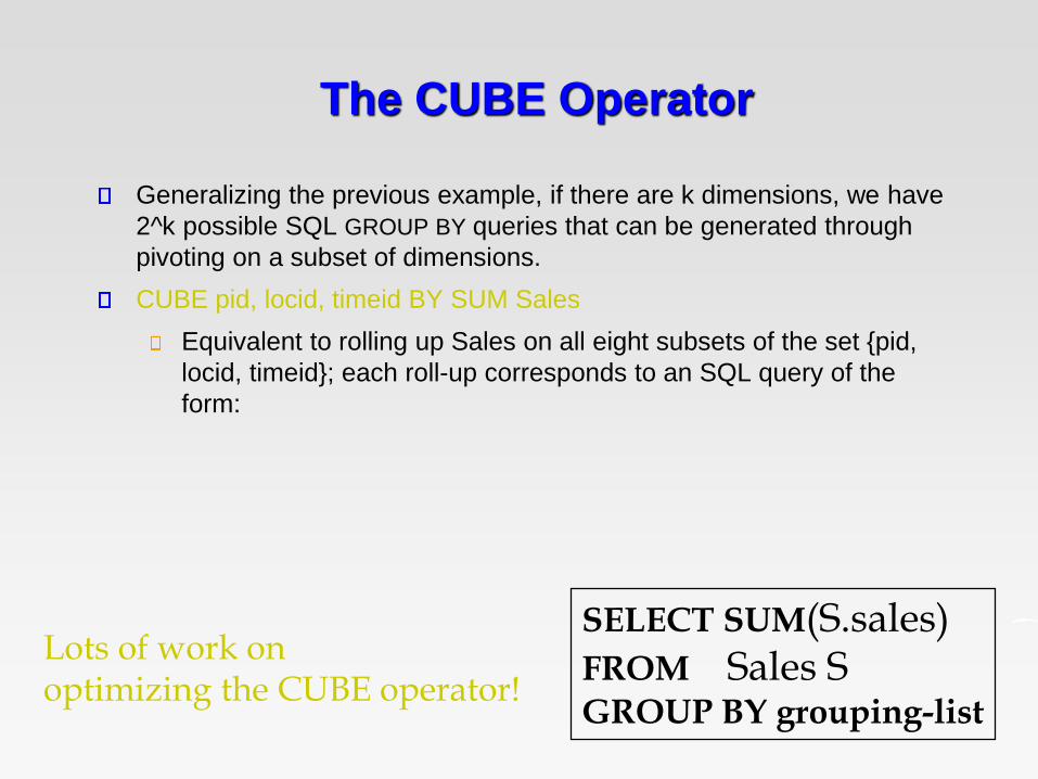
The CUBE Operator
Generalizing the previous example, if there are k dimensions, we have
2^k possible SQL GROUP BY queries that can be generated through
pivoting on a subset of dimensions.
CUBE pid, locid, timeid BY SUM Sales
Equivalent to rolling up Sales on all eight subsets of the set {pid,
locid, timeid}; each roll-up corresponds to an SQL query of the
form:
SELECT SUM(S.sales)FROM Sales SGROUP BY grouping-list
Lots of work onoptimizing the CUBE operator!

Views and Decision Support
OLAP queries are typically aggregate queries.
Precomputation is essential for interactive response times.
The CUBE is in fact a collection of aggregate queries, and
precomputation is especially important: lots of work on what is best to
precompute given a limited amount of space to store precomputed
results.
Warehouses can be thought of as a collection of asynchronously
replicated tables and periodically maintained views.
Has renewed interest in view maintenance!

View Modification (Evaluate On Demand)
CREATE VIEW RegionalSales(category,sales,state)AS SELECT P.category, S.sales, L.state
FROM Products P, Sales S, Locations LWHERE P.pid=S.pid AND S.locid=L.locid
SELECT R.category, R.state, SUM(R.sales)FROM RegionalSales AS R GROUP BY R.category, R.state
SELECT R.category, R.state, SUM(R.sales)FROM (SELECT P.category, S.sales, L.state
FROM Products P, Sales S, Locations LWHERE P.pid=S.pid AND S.locid=L.locid) AS R
GROUP BY R.category, R.state
View
Query
ModifiedQuery

View Materialization (Precomputation)
Suppose we precompute RegionalSales and store it.
Then, previous query can be answered more efficiently (modified query will
not be generated).
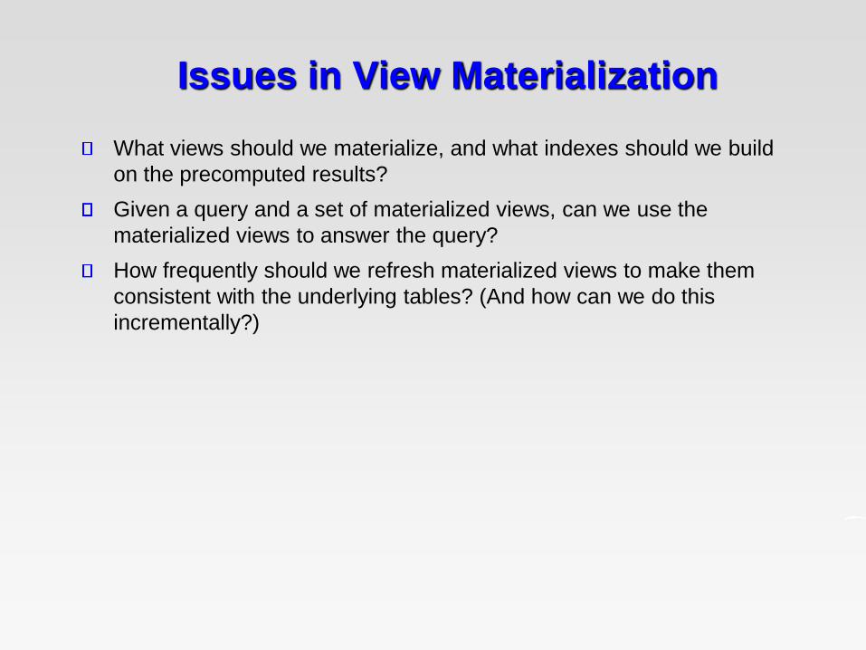
Issues in View Materialization
What views should we materialize, and what indexes should we build
on the precomputed results?
Given a query and a set of materialized views, can we use the
materialized views to answer the query?
How frequently should we refresh materialized views to make them
consistent with the underlying tables? (And how can we do this
incrementally?)
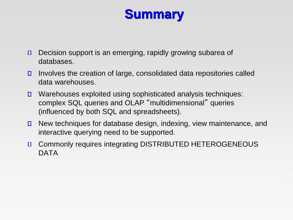
Summary
Decision support is an emerging, rapidly growing subarea of
databases.
Involves the creation of large, consolidated data repositories called
data warehouses.
Warehouses exploited using sophisticated analysis techniques:
complex SQL queries and OLAP “multidimensional” queries
(influenced by both SQL and spreadsheets).
New techniques for database design, indexing, view maintenance, and
interactive querying need to be supported.
Commonly requires integrating DISTRIBUTED HETEROGENEOUS
DATA