ocw.mit.edu · 2020-01-04 · F0 F exp λλ() ()∞= −τ λ+τ λ{⎡⎣RM() ( )⎤⎦m} (7)...

12.815, Atmospheric Radiation Dr. Robert A. McClatchey and Prof. Ronald Prinn

4. Remote Sensing A. Introduction Electromagnetic waves, interacting with a medium leave a signature dependent on the composition and thermal structure of the medium. Let M=Medium and S=Signal respectively. Then, we have: S=F(M) (1) Where F represents a function that is not necessarily linear. The function will generally relate to absorption, scattering, emission and polarization. In turn, absorption and scattering will depend on composition (molecular and particulate) and emission will depend on composition and temperature. Polarization will depend on scattering properties including the size, shape and orientation of particulates. The inverse of Eq. 1 gives: M=F-1(S) (2) Where F-1 represents the inverse of the function F. A fundamental obstacle in all inverse problems of remote sensing is the uniqueness of solution. The non-uniqueness arises because the medium under investigation may be composed of a number of unknown parameters whose various physical combinations may lead to the same radiation signature. There are also mathematical problems associated with the stability of solution. We will need to consider both active and passive remote sensing: Active Remote Sensing uses a radiation source generated by artificial means – e.g., lasers used for LIDAR or microwaves used in RADAR. Generally a beam of radiation is sent out and a back-scattered signal is measured, although it would also be possible to have the source and receiver located at different places. Range-gating enables the user to determine the location of scatterers. Passive Remote Sensing uses natural radiation sources such as the sun or the emission of the earth and atmosphere itself. Thus, wavelengths of the solar spectrum from the UV to the IR are accessible and thermal emission by the earth atmosphere system is available from about 4 μm to the far infrared and microwave region. B. Scattered Sunlight as a Means of Remote Sensing Consider sunlight incident on the top of the atmosphere with a measurement system located at the earth’s surface. We have:

( ) ( ) ( ) ( ) ( ) ( )λ λ ⎡ ⎤= − θ λ ρ + σ λ + σ λ⎣ ⎦R M

0 s edF (z) F (z)dz sec k z N z N za (3)

12.815, Atmospheric Radiation Lecture Dr. Robert A. McClatchey and Prof. Ronald Prinn of 29

where is solar zenith angle. 0θ k is absorption coefficient associated with molecules. ρ is the density of molecular absorbers.

σ is the Rayleigh scattering cross-section. Rs

= number of molecules/cm( )N z 3 at height z.

( )aN z = number of aerosols/cm3 at height z.

σ = Mie extinction cross-section λMe ( )

The solution to Eq. 3 is as follows:

( )( ) ( ) ( ) ( ) ( )λ

λ ∞

⎡ ⎤= − λ ρ θ − λ θ − λ θ⎢ ⎥

∞⎢ ⎥⎣ ⎦τ τ∫

0R M

o o

F 0ln k z sec dz sec sec

F o (4)

where we have introduced the optical depths associated with Rayleigh and Mie extinctions as τR and τM respectively. Let us consider the example of seeking the total ozone concentration in the atmosphere so that k(λ) is the absorption coefficient due to ozone at wavelength λ and ρ(λ) is the density of ozone at altitude z. The total ozone concentration will then be:

( ) ( )∞

∞

= ρ = ρΩ ∫ ∫0

0

z dz z dz (5)

Let us also simplify our problem by recognizing that ozone is concentrated in a layer centered near 22 km, so we can set θo = Z where Z = the solar zenith angle at 22 km. Otherwise, we’ll use m = sec θo. If we now select two wavelengths (λ1 and λ2) in the Hartley-Huggins ozone absorption band where there is little absorption by other atmospheric molecules and if we assume that the aerosol optical depths are about the same at these two wavelengths we can evaluate Eq. 4 for each wavelength. Subtracting the equation for λ2 from the equation for λ1 then enables a solution for Ω.

( ) ( ) ( ) ( ) ( ) ( )( ) ( )

λ λ λ λ ⎡ ⎤⎡ ⎤ ⎡ ⎤∞ ∞ − − τ λ − τ λ⎣ ⎦ ⎣ ⎦ ⎣ ⎦=⎡ ⎤λ − λ⎣ ⎦

ΩR R

1 2 1 2 1 2

1 2

ln F F ln F 0 F 0 m

sec Z k k (6)

In this equation, everything is known except ( ) ( )λ λ1 2F 0 F 0 which can be measured at the

surface. The determination of this quantity is routinely measured via a standard instrument known as a Dobson spectrometer at 80 ground stations around the world. Turbidity Detection Turbidity is a measurement of atmospheric aerosols, both natural and manmade. Let us write Eq. 3 for the situation where molecular absorption is ∼ 0. The solution of Eq. 4 then becomes:


( ) ( ) ( ) ( ){ }λ λ ⎡∞ = − τ λ + τ λ⎣R MF 0 F exp m⎤⎦ (7)

( )τ λR can be theoretically calculated, enabling us to solve Eq. 7 for ( )τ λM . The quantity, ( )τ λM ,

depends on the number of particles and the particle size distribution. The solution for either requires an assumption for the other. So, we cannot truly obtain a unique solution here. Water Vapor Determination Measurement of incoming solar flux at two wavelengths in a near infrared water vapor band can be used to determine the total amount of precipitable water in the path from sun to ground. In this case, Eq. 4 outside of the water band becomes:

( ) ( ) ( ) ( ){ }λ λ ⎡∞ = − τ λ + τ λ⎣M R

1 1 1 1F 0 F exp m⎤⎦ (8)

The solution to Eq. 4 in the water vapor band is similarly given by Eq. 9:

( ) ( ) ( ) ( ){ }λ λ ⎡ ⎤∞ = − τ λ + τ λ −⎣ ⎦M R

2 2 2 2F 0 F exp m K um (9)

where 0K S= π α δ , with So the mean line intensity, α the mean line half-width and δ the

mean line spacing. The path length (or precipitable water) is represented by u. If we assume that the extinction of molecules and aerosols is about the same at these 2 wavelengths, we can divide Eq. 9 by Eq. 8 and obtain Eq. 10.

( ) ( )( ) ( ) { }λ λ

λ λ

∞= − μ =

∞2 2 0

1 1

F 0 F qexp K m

F 0 F q∞

(10)

∞

⎛ ⎞⎜ ⎟⎝ ⎠=

2

0

2

qln

qu

K m where 2 1

2 1

0 (0) / (0)

( ) / ( )

q F F

q F Fλ λ

λ λ∞

=

= ∞ ∞ (11)

Reflected Sunlight Extinction can also be used to determine the amount of an absorbing gas in the atmosphere by making measurements at two wavelengths, appropriately spaced in an absorption band and outside of the absorption band. However, in this case we will consider the scenario of a satellite viewing the earth at the angle whereas the sunlight is incident on the atmosphere at angle

. The solution to Eq. 3 now requires slight modification as indicated in Eq. 12: θs

θo

( )( ) ( ) ( ) ( ) ( ) ( ) ( )

0R R

0 s 00

F tln k z sec dz k z sec dz sec sec

F

∞λ

λ ∞

⎡ ⎤ ⎡ ⎤s⎡ ⎤= − λ ρ θ + λ ρ θ − τ λ θ + τ λ θ⎢ ⎥ ⎢ ⎥ ⎣ ⎦∞⎢ ⎥ ⎣ ⎦⎣ ⎦

∫ ∫

( ) ( )M M0 ssec sec⎡ ⎤− τ λ θ + τ λ θ⎣ ⎦ (12)

Selecting 2 wavelengths in an absorption band sufficiently closely spaced in wavelength that Rayleigh and Mie extinction and surface (or cloud-top) reflection can be considered independent


of wavelength, but with an appreciable difference in absorption by a molecular component of the atmosphere (such as ozone or water vapor), we can write two equations again take the difference and obtain Eq. 13:

( ) ( ) ( ) ( ) ( ) ( ) ( ) ( )∞

λ λ λ λ∞

⎡ ⎤− ∞ − + ∞ = − λ ρ θ + λ ρ θ⎢ ⎥

⎣ ⎦∫ ∫1 1 2 2

0

1 0 10

lnF t lnF lnF t lnF k z sec dz k z sec dzs

s z

( ) ( ) ( ) ( )∞

∞

⎡ ⎤+ λ ρ θ + λ ρ θ⎢ ⎥⎣ ⎦∫ ∫0

2 o 20

k z sec dz k z sec d (13)

and if is independent of z and since , we have: ( )λk ( ) ( )∞

∞

ρ = ρ∫ ∫0

0

z dz z dz

( )( )

( )( ) ( ) ( ) ( ) ( )λ λ

λ λ

⎡ ⎤ ⎡ ⎤∞− = − Ω λ θ + θ + Ω λ θ + θ⎢ ⎥ ⎢ ⎥

∞⎢ ⎥ ⎢ ⎥⎣ ⎦ ⎣ ⎦

1 1

2 2

1 0 s 2 0

F t Fln ln k sec sec k sec sec

F t F s (14)

Again, the ratio ( ) ( )λ λ∞1 2F F ∞

2

is known from measurements of the solar constant,

are known from laboratory spectroscopic measurements, and θ are

determined from the time of day and geometry of measurement,

( ) ( )λ λ1k & k θ0 s

( ) ( )λ λ1 2F t F t are measured by

the satellite and Ω is the integrated abundance of the atmospheric gas in question. Notice that the procedure will not work if ( )λk is dependent on z.

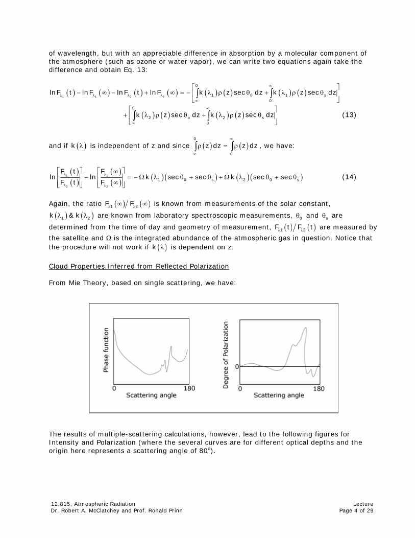
Cloud Properties Inferred from Reflected Polarization From Mie Theory, based on single scattering, we have:

The results of multiple-scattering calculations, however, lead to the following figures for Intensity and Polarization (where the several curves are for different optical depths and the origin here represents a scattering angle of 80o).


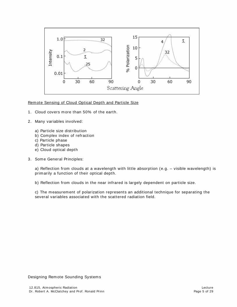
Remote Sensing of Cloud Optical Depth and Particle Size 1. Cloud covers more than 50% of the earth.

2. Many variables involved:

a) Particle size distribution b) Complex index of refraction c) Particle phase d) Particle shapes e) Cloud optical depth

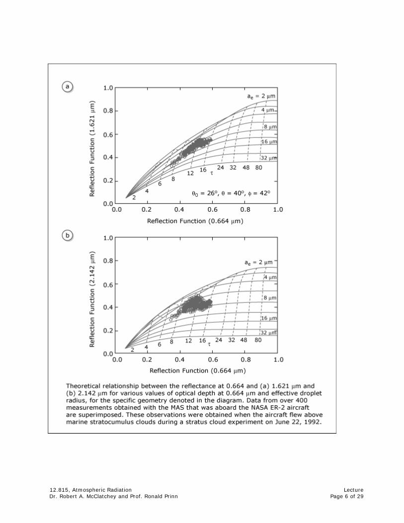
3. Some General Principles: a) Reflection from clouds at a wavelength with little absorption (e.g. – visible wavelength) is primarily a function of their optical depth. b) Reflection from clouds in the near infrared is largely dependent on particle size. c) The measurement of polarization represents an additional technique for separating the several variables associated with the scattered radiation field.

Designing Remote Sounding Systems


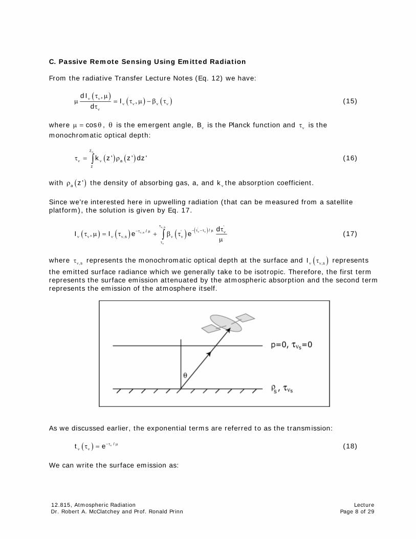
C. Passive Remote Sensing Using Emitted Radiation From the radiative Transfer Lecture Notes (Eq. 12) we have:

( ) ( ) (ν νν ν ν ν

ν

τ μ)μ = τ μ − β τ

τ

dI ,I ,

d (15)

where μ = , is the emergent angle, θcos θ νB is the Planck function and is the monochromatic optical depth:

ντ

( ) ( )z

az

k z ' z ' dz '∞

ν ντ = ρ∫ (16)

with ( )ρa z ' the density of absorbing gas, a, and kν the absorption coefficient.

Since we’re interested here in upwelling radiation (that can be measured from a satellite platform), the solution is given by Eq. 17.

( ) ( ) ( ) ( )ν

ν νν

ν

τ− τ −τ μ−τ μ ν

ν ν ν ν ν ντ

ττ μ = τ + β τ

μ∫,s '

,s

'// '

,s

dI , I e e (17)

where represents the monochromatic optical depth at the surface and represents

the emitted surface radiance which we generally take to be isotropic. Therefore, the first term represents the surface emission attenuated by the atmospheric absorption and the second term represents the emission of the atmosphere itself.

ντ ,s (ν ντ ,sI )

As we discussed earlier, the exponential terms are referred to as the transmission:

( ) ν−τ μν ντ = /t e (18)

We can write the surface emission as:


( ) ( )ν ν ν ντ μ = βε,s sI , T (19)

where is the surface temperature and where sT νε is the emissivity which can be taken = 1 in much of the thermal infrared region. It is also customary to define a “weighting function” by:

( ) ν−τ μν ν

ν

τ −=

τ μ

/dt ed

(20)

Thus the radiance at the top of the atmosphere is given by:

( ) ( ) ( ) ( ) ( )ν

ν νν ν ν ν ν

ντ

∂ τνμ = β τ + β τ

∂ τ∫,s

0

s ,s

tI 0, T t dτ (21)

In remote sensing, we usually write Eq. 21 in terms of height or pressure as independent variable. Let us define:

a ad k dz k q dzν ν ντ = − ρ = − ρ (22a)

ak q d dSince g

g dzν ρ ρ⎛= ⎜

⎝ ⎠⎞= −ρ ⎟ (22b)

where = absorber mass mixing ratio. We can then write Eq. 21 in terms of pressure as follows:

aq

( ) ( ) ( ) ( )( ) ( )s

0

s ,sp

t pI 0, T t T p dp

pν

ν ν ν ν ν

∂μ = β τ + β

∂∫ (23)

where is now the surface pressure. sp An instrument capable of measuring radiance as a function of frequency (or wavenumber)

always has a finite bandwidth, ( )ν νΨ

, where Ψ is the instrument response function and ν its

mean frequency (wavenumber). The measured radiance is then given by Eq. 24:

( ) ( )ν ν

ννν ν

= Ψ ν ν ν Ψ ν ν ν∫ ∫2 2

1 1

I I , d , d (24)

Since the Planck function varies slowly with frequency compared with the spectral response of a spectrometer, we can consider it to be constant over the interval Δν = ν − ν2 1 Therefore, if we now integrate Eq. 23 over the frequency interval, Δν we obtain Eqs 25 & 26.


( ) ( ) ( ) ( ) ( )ΔνΔνν ν ν

∂⎡ ⎤μ = + ⎣ ⎦ ∂∫

s

0

s sp

t pI 0, B T t p B T p dp

p (25)

or ( ) ( ) ( ) ( )( )

( )Δν

Δν Δνν ν ν⎡ ⎤μ = + ⎣ ⎦∫

s

1

s st p

I 0, B T t p B T p dt p (25a)

where ( )( ) ( ) ( )

( )

ν

νν

Δν ν

ν

⎡ ⎤Ψ ν ν −⎢ ⎥

⎢ ⎥⎣ ⎦=

Ψ ν ν ν

∫ ∫

∫

2

1

2

1

p

0

1, exp k p ' q p ' dp '

gt p

, d

(26)

Summary

1. The upwelling radiance has 2 components a) Surface term b) Atmospheric term

2. Temperature information is included in the Planck function whereas, absorbing gas profile information is included in the atmospheric transmission.

3. Observed radiances relate in a complex and inter-related way to the temperature and molecular constituent profiles in the atmosphere.

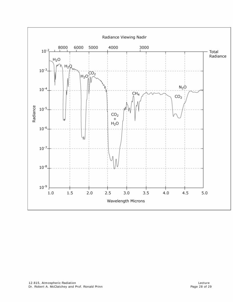
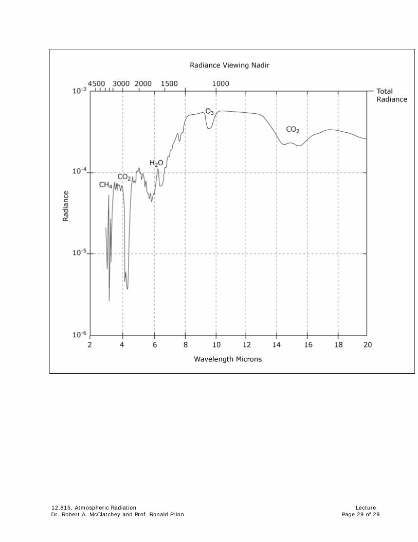
Choice of spectral regions for downward viewing

i. Available gaseous absorbers (thermal infrared)

( )λ μm Gas Applications

4.4–4.6 N2O(ν3 ) air temperature – tropo. 4.18–4.5 CO2(ν3 ) air temp. – tropo., strato. 13–18 CO2(ν2 ) air temp. – tropo., strato. 4300–5900 (5 mm) O2 air temp. – strato, meso. 5–8.3 H2O(ν2 ) H2O abundance 12.5–13,500 H2O(rot’n) H2O abundance 9–10 O3(ν3 ) ozone abundance 13.3–15.4 O3(ν2 ) ozone abundance 3.5–4.18 window (no gas) surface & cloud-top temp. 10–13 window (no gas) surface & cloud-top temp. 7,000–11,000 window (no gas) surface & cloud-top temp. >15,000 window (no gas) surface & cloud-top temp.


ii. Free of interference from clouds and aerosols (e.g., microwave region).

iii. Maximum energy emission – strongly peaked near 15 μm (emission intensities are normalized.)

( )λ μm 200 K 300 K

4.3 1.25 200 15.0 5000 15,000 5 mm 1 1 iv. Detector performance (normalized = emission intensity signal/detector noise signal)

( )λ μm 200 K 300 K

4.3 1 20 15 10 6 5 4 1 (i.e. – at 300K, 4.3 is best and at 200K, 15 is best.)

v. Redundancy – because each spectral radiance measurement comes from a range of altitude, we can get redundancy.

D. Temperature Sounding using the 15 μm CO2 Band Let us specialize our problem to temperature sounding and the use of a CO2 band for this purpose. And let us assume a spectral measurement over a 10 cm-1 bandpass. We can reasonably assume that carbon dioxide is uniformly mixed in the atmosphere in the altitude regime we’re interested in (0-40 km). This means that

0m C pΔ = Δ or (measuring down from the top of the atmosphere), 0m C p= Returning to the solution to the Radiative Transfer Equation on page 8,

( ) ( ) ( ) ( )( ) ( )ν ν ν ν νμ = μ + μ∫

s

0

s sp

I 0, B T t ,p B T p dt ,p dp

let us define a weighting function as νdt dlnp and perform our integration over ln which is similar to z. And let us consider vertical viewing so we can for now ignore the μ dependence.

p

In order for the average transmission over 10 cm-1 to be significant (say transmission between 0.1 and 0.9), individual absorption lines will generally be completely absorbed at their centers and can be associated with the limiting case of strong absorption. As we showed earlier (See MODTRAN Lecture notes), for this


situation, ( )Δν ν⎛ ⎞= − α⎜ ⎟⎝ ⎠

∑1 1i i 2 2

Li

t exp 2 S m

where = intensity per unit mass of the iνiS th line

α = Lorentz width of the iiL

th line (α = αi iL Lo

o

pp )

m = mass of absorbing gas in the path Since is proportional to pressure and m is also proportional to pressure, we have: i

Lα

t exp A pΔν Δν= −⎡⎣ ⎤⎦ from the top of the atmosphere to the pressure level, p.

Computing the Weighting Function, we obtain:

ApdtW A pe

dlnp−

Δν= =

And the weighting Function maximum can be determined:

( )− −= − + =

2Ap 2 2 Ap

2

d tApe A p e 0

d lnp Max is at A=1/p

Thus we have . This value is reached when p=1/A. −= =1W e 0.368 We can select spectral bands such that we achieve an array of weighting functions that span the atmosphere and are distributed in a reasonable manner.


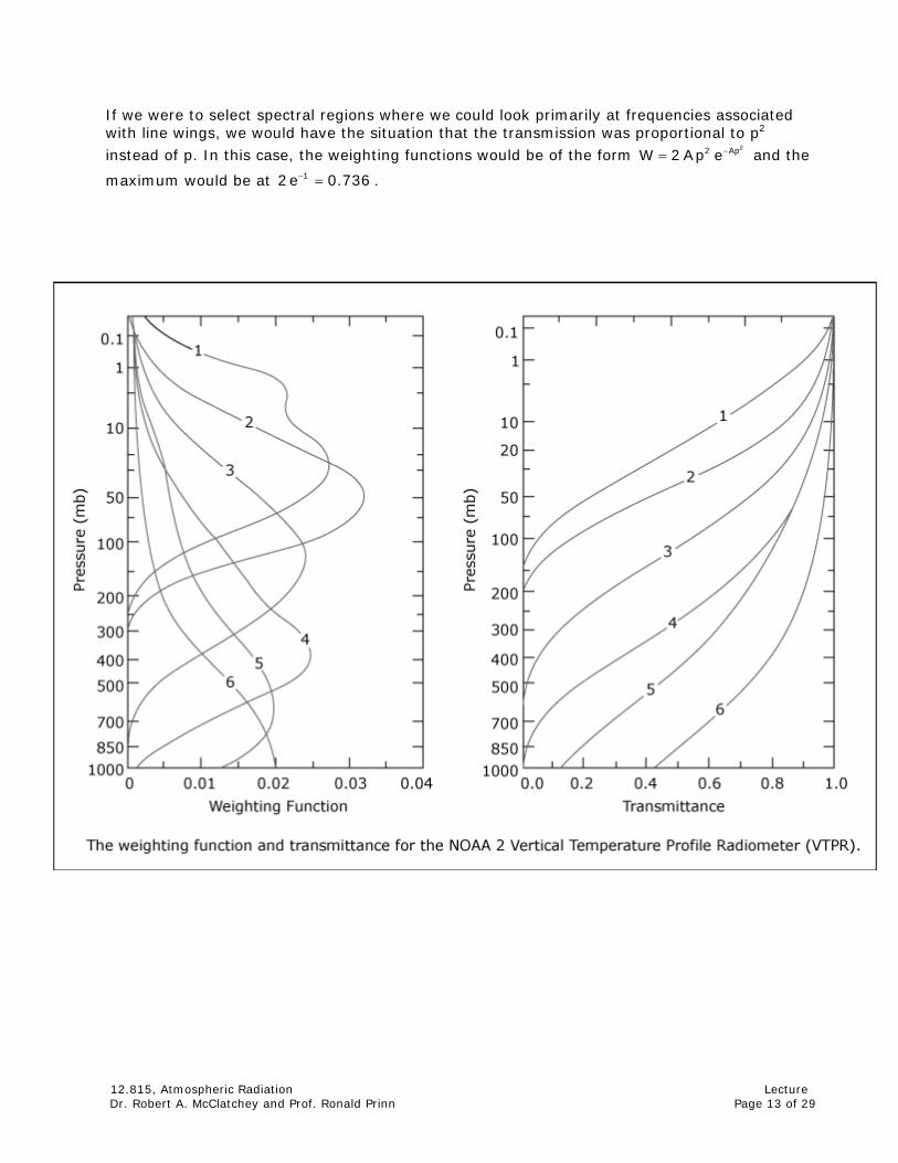
If we were to select spectral regions where we could look primarily at frequencies associated with line wings, we would have the situation that the transmission was proportional to p2 instead of p. In this case, the weighting functions would be of the form and the

maximum would be at .

−=22 ApW 2 Ap e

− =12e 0.736


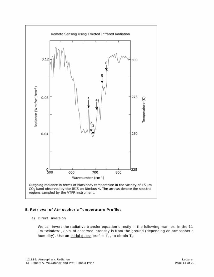
E. Retrieval of Atmospheric Temperature Profiles

a) Direct Inversion

We can invert the radiative transfer equation directly in the following manner. In the 11 μm “window”, 85% of observed intensity is from the ground (depending on atmospheric humidity). Use an initial guess profile pT , to obtain Ts:


( ) ( ) ( ) ( )( )

( )Δν μ

ν ννν νμ = μ + μ∫

st p

ps s1

B T t ,p I ,0 B T dt ,p (27)

(obs. At 11 μm) Usually, pT is climatological mean or better, a “forecast”. Now put

( ) ( ) ( )ν

ν ν= +

p

pp p

dB TB T B T h

dT (Taylor approximation)

− ppT T

Thus, defining the observable, ( )r

νμ (for all otherν ).

( ) ( ) ( )r I ,0 Iνν ν

μ = μ − μ,0

(observed) (guess)

( ) ( ) ( ) ( )( )

( )Δν μ

Δν Δννν ν= μ − μ + μ∫

st p

ps s1

I ,0 B T t ,p B T dt ,p

( )( ) ( )ν μ νΔν= − μ∫

spt p

p1

dB Th dt ,p

dT

where we have used Equation 25a. We can now approximate the integral with a summation:

= =

∂= =

∂∑ ∑N N

ii ij j

j 1 j 1 j

rjh h

hr a (29)

where i is and j is P, z, or ν νt .

Thus r =Ah; where A is a “partial derivative” matrix and h=A-1 r gives temperature profile by “direct inversion”. Unfortunately, this method requires a precise knowledge of tΔν which is not available from first principles (due to a lack of knowledge of atmospheric composition – especially, in terms of water vapor and clouds). Without this precise result, our efforts to retrieve the temperature profile by direct inversion will likely result in failure.

b) Indirect Inversion – empirical regression method – here, no transmission functions are required. Entirely empirical.

--L pairs of radiosonde temperature and satellite rediance measurements are available at the same point.


--define H = [hjk] j = 1, N ; k = 1, L and R = [rik] i = 1, M ; k = 1, L

pressure levels of radiosondes

number of pairs

frequencies of radiance measurements

where as before hjk = h (pj)k = T(pj)k - ( )jT p

a guess-for example, the mean of all radiosonde temperatures at pj

rik = r ( )iν k = I( )iν k - ( )iI ν

a guess-for example, the mean of all L satellite radiances at νi.

Here, we will correlate temperature profiles with radiances in a Least Square Sense. Now, assume a linear relation between H and R. (N x L) (N x M) (M x L) (N x L) H = C R or O = H – C R(error matrix)

Define = = =

⎛ ⎞= −⎜ ⎟

⎝ ⎠ε ∑ ∑ ∑

2N L M

jk ji ikj 1 k 1 i 1

h C r

known (needed) known = t r ([H – C R] [H – C R]’)

sum of all

diagonal elements “Error Covariance” matrix

where the prime represents the transpose matrix. Ideally want =ε 0 ; therefore minimize to obtain best C in a least Squares sense.

i.e. want 2L M

jk ji i kk 1 i 1ji ji

h C rC C

∗ ∗∗= =

⎧ ⎫⎛ ⎞∂ ε ∂ ⎪ ⎪= −⎨ ⎬⎜ ⎟∂ ∂ ⎝ ⎠⎪ ⎪⎩ ⎭∑ ∑

( )∗ ∗∗= =

⎛ ⎞= −⎜ ⎟

⎝ ⎠∑ ∑L M

jk iji i kk 1 i 1

2 h C r rk


( ) ( )∗ ∗∗= =

⎡ ⎤⎡ ⎤= −⎢ ⎥⎢ ⎥

⎣ ⎦⎣ ⎦∑ ∑L M

jk ki kiji i kk 1 i 1

2h r ' 2 C r r '

= j ith element of 2HR’-2CRR’ = 0 for all j and i

(NxM) (NxM) (MxM) i.e. 2HR’-2CRR’=0 and C = HR ‘ (R R’)-1

where the ‘ indicates the “transpose matrix”. ij element ( )L

ik kjk 1

r r '=∑ co-factor matrix

of RR’ |RR’|

To prevent RR’ (MxL, LxM) being singular, generally want L>>M, i.e. many more IR sounder-radiosonde coincidences than wavelengths – i.e. no redundant radiosonde-sounding coincidences. We can now use this empirically – derived C (compare to the transmission function matrix, A-1 above) to invert all other satellite soundings:

i.e. h Cr=

F. Remote Sensing Exercise A 2-part Remote Sensing Exercise will be handed out here. The first part deals with temperature retrieval by empirical regression. The second part asks you to again use the MODTRAN code to examine weighting functions in the 15 μm band of CO2 and use the information to design a system for temperature sounding. G. Temperature Retrieval Based on Iteration The retrieval procedures we’ve discussed so far are linear and empirical. The problem we face here is that the radiative transfer equation (a Fredholm equation with fixed limits) may not always have a solution. The radiances contain experimental uncertainty and so do the calculated transmission results. Furthermore, it is necessary to approximate the integral by a sum, again introducing errors in the computed radiances. We should instead consider a non-linear approach. Re-writing the solution to the equation of radiative transfer, we have:

( ) ( ) ( ) ( )∂⎡ ⎤= + ⎣ ⎦ ∂∫

s

0i

ii i s s ip

t pB T t p B T p dlnp

lnpI (28)

where we’ve used ln p as independent variable and where i denotes the spectral channels. Using the mean value theorem, the radiance can be approximated by Eq. 29.


( ) ( ) ( ) ( )⎡ ⎤∂⎡ ⎤− ≅ ⎢ ⎥⎣ ⎦ ∂⎢ ⎥⎣ ⎦

ii ii s s i i i

t pB T t p B T p lnp

lnpI Δ (29)

where pi denotes the pressure level at which the maximum weighting function is located and is the pressure difference at the ith level and is defined as the effective width of the

weighting function. If the guessed temperature profile is T*(p), the expected radiance is then given by Eq. 30.

i lnpΔ

( ) ( ) ( ) ( )∗∗∗ ∗

⎡ ⎤∂⎢ ⎥⎡ ⎤− = ⎣ ⎦ ⎢ ⎥∂⎣ ⎦

i

ii i s s i i i

P

t pI B T t p B T p lnp

lnpΔ (30)

Dividing Eq. 29 by Eq. 30 then leads to Eq. 31:

( ) ( )( ) ( )

( )( )( )( )∗ ∗ ∗

−≅

−i i i ii s s

i i s i s i i

B T pI B T t p

I B T t p B T p (31)

At frequencies where the surface contribution to the upwelling radiance is small, Eq. 31 may be approximated by Eq. 32.

( )( )∗ ∗

⎡ ⎤⎣≅⎡ ⎤⎣ ⎦

i i i

i i

B T pII B T p

⎦ (32)

This approach was pioneered by M. Chahine and is referred to as the relaxation equation. A number of variants of this procedure have been developed and are used operationally today. Here is the recipe for applying this kind of procedure. The quantity, n, is used here to represent the order of iteration. 1. Make an initial guess for the temperature profile: ( ) ( )n

iT p , n = 0

2. Substitute T(n) into Eq. 28 and use an accurate quadrature formula to compute the expected

upwelling radiance for each sounding channel.

( )niI

3. Compare the computed radiance values with the measured data . If the residuals ( )niI iI

( )n

i ini

i

I IR

I

−= are less than a preset small value (e.g., 10-4) for each sounding channel, then

T(n) is a solution. If not, continue the iteration.

4. Apply the relaxation equation (Eq. 32) M (where M = number of spectral channels, and we have the same number of pressure levels as spectral channels) times to generate a new guess for the temperature values T(n+1)(pi) at the selected i pressure levels, i.e., force the temperature profile to match the observed radiances. Since the Planck function can be written as Eq. 33 with a = 2hc2 and b= hc/k


( ) ( )νν=

−i

3i

i b TaB T

e 1 (33)

we can write an iterative equation for the temperature in terms of the previous iteration as indicated in Eq. 34.

( )( ) ( ) ( )( ) ( ){i

n 1 n nii i ip b ln 1 1 exp b T p I IT + ⎡= ν − − ν⎣ }i

⎤⎦

(34)

i = 1, 2 ……... M

5. Carry out the interpolation between the temperature value at each given level, pi, to obtain the desired profile.

6. Finally, go back to step 2 and repeat until the residuals are less than the preset criterion. How well will the relaxation method converge to the correct solution? Or will it fail to converge? A variety of testing has led to variants of this procedure that are used in practice. H. Water Vapor Retrieval Based on Iteration Let us go back to the solution of the Eq. Of Radiative Transfer Equation as expressed in Eq. 25 (repeated here as Eq. 35):

( ) ( ) ( ) ( ) ( )ΔνΔνν ν ν

∂⎡ ⎤μ = + ⎣ ⎦ ∂∫

s

0

s sp

t pI 0, B T t p B T p dp

p (35)

Performing an integration by parts on Eq. 35, we obtain Eq. 36.

( )( ) ( ) ( )νΔνν ν

∂= −

∂∫s

0

p

B pI B T 0 t p d

pp (36)

Where T(0) denotes the temperature at the top of the atmosphere and the spectral transmission is given by Eq. 37.

( ) ( ) ( )P

0

dt p exp k p dm pΔν ν

Δν

⎡ ⎤ ν= −⎢ ⎥ Δν⎣ ⎦∫ ∫ (37)

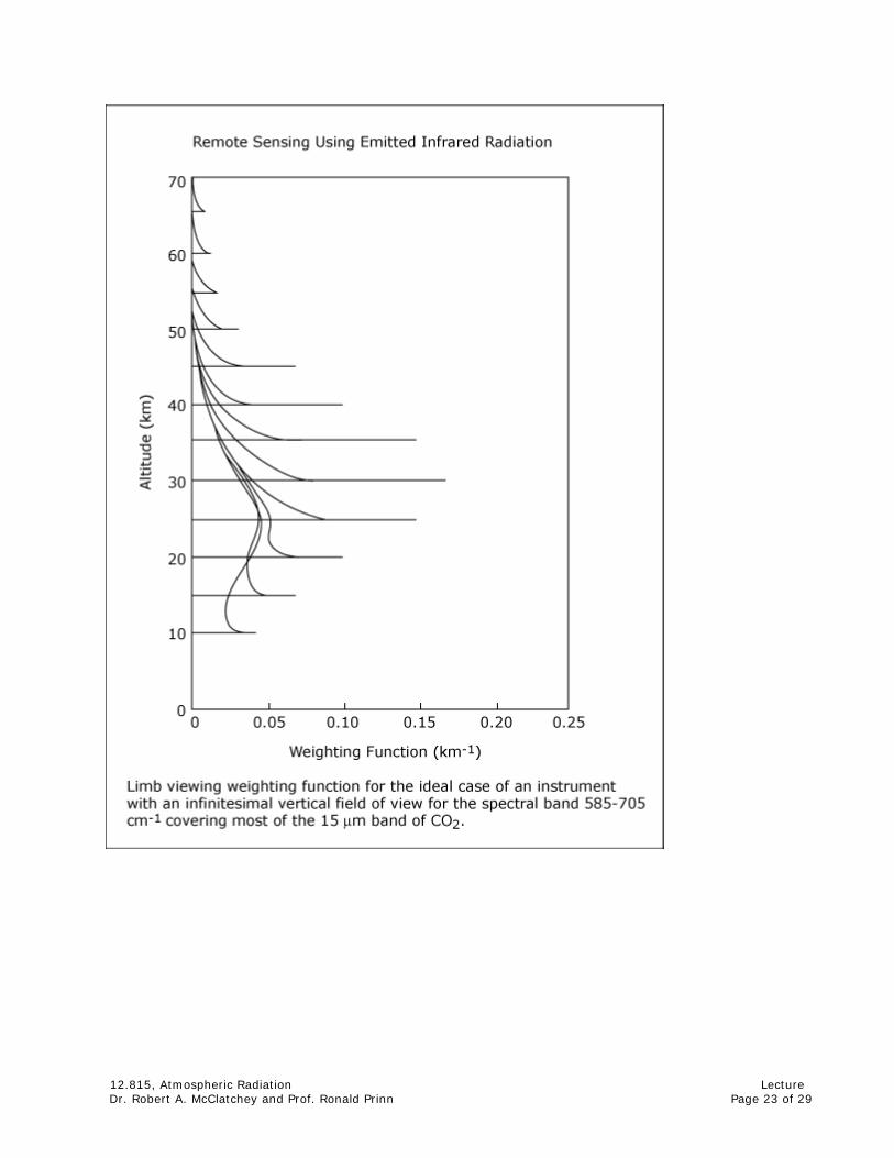
If the temperature profile has been retrieved through measurements in one of the CO2 bands, then the remaining unknown is the transmission. We can then select spectral channels in an appropriate water vapor absorption band (e.g. – the 6.3 micrometer vibration-rotation band) and attempt to retrieve the concentration of water along the path. Empirical procedures have been used with some success and more recently, iterative procedures are being applied. However, the accuracy of retrieval is poorer than for temperature retrieval and is generally in the range of 10-20%. Higher spectral resolution measurements of the future are thought to enable measurements somewhat better than 10%. I. Limb Sounding


1. Useful for measuring trace constituent profiles of the middle atmosphere 10 ≤ Z ≤ 60 km.

2. Can look at transmission (absorption) or emission. Transmission measurements are limited

by availability of the sun and so only occasional occultations are observed.

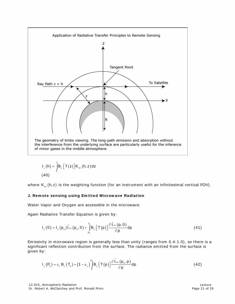
3. Emission measurements (in thermal infrared) can be made any time of day or night. a) Emission originates in the few km immediately above tangent point due to rapid decrease of atmospheric density and pressure. This, coupled with low-altitude cut-off leads to an inherent high vertical resolution of measurement. b) All radiation comes solely from atmosphere – no surface boundary contribution. c) Horizontal (tangent) path leads to high opacity (x37). Thus, it is good for minor gas detection. d) Disadvantages: 1) High clouds; and 2) Horizontal region sounded is large (~ 100-200 km).

Eq. Of Radiative Transfer for Limb Infrared Emission:

( ) ( ) ( ) ( )ΔνΔνν ν ν

∂⎡ ⎤= + ⎣ ⎦ ∂∫

s

0

s sp

t p,0I B T t p B T p d

pp (38)

Specializing radiative transfer equation to limb situation, we have:

( ) ( ) ( )+∞Δν

ν ν−∞

∂ χ⎡ ⎤= ⎣ ⎦ ∂ χ∫

t h,I h B T X dχ (39)

where the boundary term has been set = 0 and the independent variable has been converted to x. For determining gaseous composition as a function of height (z), we must change variable from x to z (using spherical geometry). We then have:


( ) ( ) ( )∞

Δνν ν⎡ ⎤= ⎣ ⎦∫

0

I h B T z K h,z dz

(40) where ( )K h,zΔν is the weighting function (for an instrument with an infinitesimal vertical FOV).

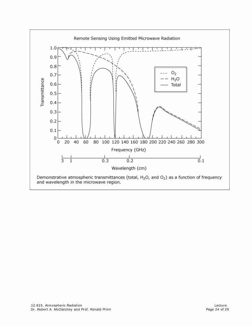
J. Remote sensing using Emitted Microwave Radiation Water Vapor and Oxygen are accessible in the microwave. Again Radiative Transfer Equation is given by:

( ) ( ) ( ) ( ) ( )ΔνΔνν ν ν

∂⎡ ⎤= + ⎣ ⎦ ∂∫

s

0

s sp

t p,0I 0 I p t p ,0 B T p dp

p (41)

Emissivity in microwave region is generally less than unity (ranges from 0.4-1.0), so there is a significant reflection contribution from the surface. The radiance emitted from the surface is given by:

( ) ( ) ( ) ( ) ( )Δν

ν ν ν ν ν

∂⎡ ⎤= ε + − ε ⎣ ⎦ ∂∫

sps

s s0

t p ,pI P B T 1 B T p dp

p (42)


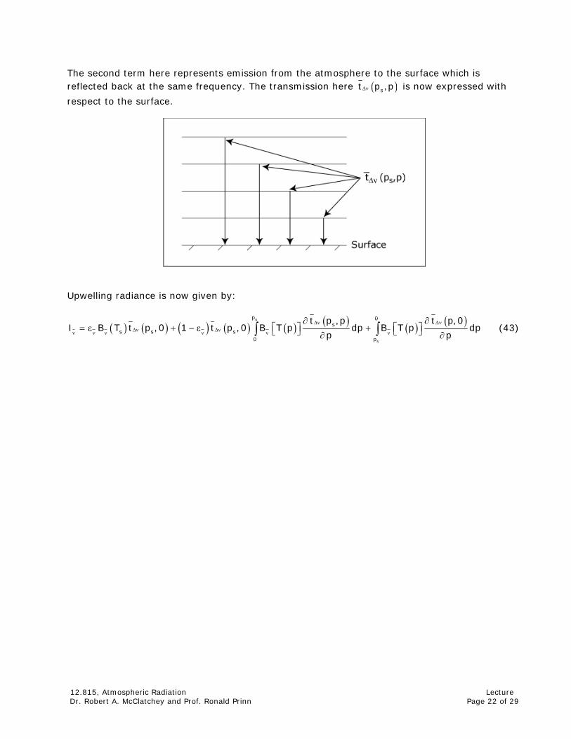
The second term here represents emission from the atmosphere to the surface which is reflected back at the same frequency. The transmission here ( )st p ,pΔν is now expressed with

respect to the surface.

Upwelling radiance is now given by:

( ) ( ) ( ) ( ) ( ) ( ) ( ) ( )Δν ΔνΔν Δνν ν ν ν ν ν

∂ ∂⎡ ⎤ ⎡ ⎤= ε + − ε +⎣ ⎦ ⎣ ⎦∂ ∂∫ ∫

s

s

p 0s

s s s0 p

t p ,p t p,0I B T t p ,0 1 t p ,0 B T p dp B T p d

p pp (43)


In the microwave region we have that hc hT 1ν << . Therefore ( ) ν −

ν⎡ ⎤= ν ν⎣ ⎦

3 hc kt 1 2B T 2hc e 2k T (44)

as we are in spectral region where the Rayleigh-Jeans Law applies. This very good approximation then leads to the following:

( ) ( ) ( ) ( ) ( ) ( ) ( ) ( )Δν ΔνΔν Δνν ν

∂ ∂ν = ε + − ε +

∂ ∂∫ ∫s

s

p 0s

B s s s0 p

t p ,p t p,0T T t p ,0 1 t p ,0 T p dp T p

p pdp (45)


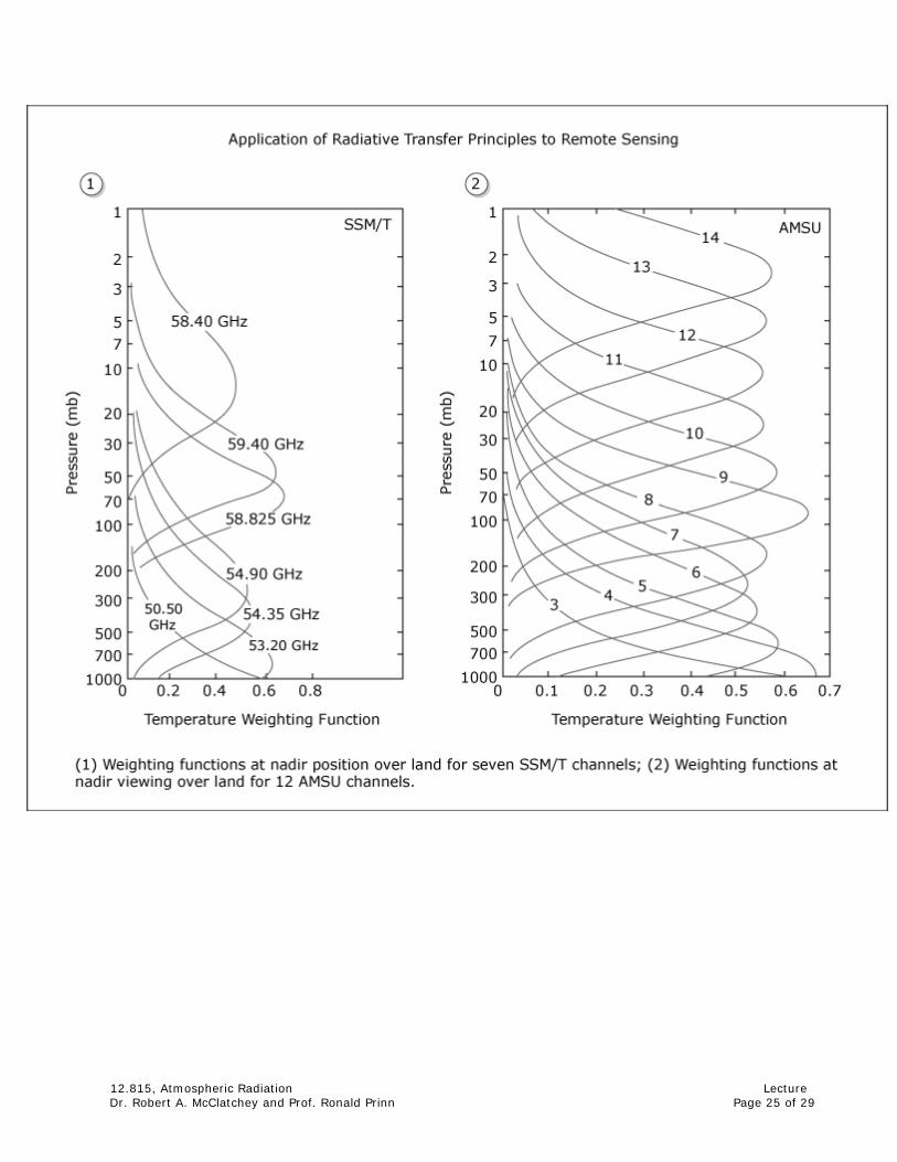
L. Designing Remote Sounding Systems


ocw.mit.edu · 2020-01-04 · F0 F exp λλ() ()∞= −τ λ+τ λ{⎡⎣RM() ( )⎤⎦m} (7)...

Documents

Transcript of ocw.mit.edu · 2020-01-04 · F0 F exp λλ() ()∞= −τ λ+τ λ{⎡⎣RM() ( )⎤⎦m} (7)...