Clemson UniversityTigerPrints

All Theses Theses

8-2018

Observing the Gamma-Ray Burst–SupernovaConnection with 1m-class Aperture TelescopesCorinne Maly TaylorClemson University, corinn4@clemson.edu

Follow this and additional works at: https://tigerprints.clemson.edu/all_theses

This Thesis is brought to you for free and open access by the Theses at TigerPrints. It has been accepted for inclusion in All Theses by an authorizedadministrator of TigerPrints. For more information, please contact kokeefe@clemson.edu.

Recommended CitationTaylor, Corinne Maly, "Observing the Gamma-Ray Burst–Supernova Connection with 1m-class Aperture Telescopes" (2018). AllTheses. 2904.https://tigerprints.clemson.edu/all_theses/2904

Observing the Gamma-Ray Burst–Supernova Connectionwith 1m-class Aperture Telescopes

A Thesis

Presented to

the Graduate School of

Clemson University

In Partial Fulfillment

of the Requirements for the Degree

Master of Science

Physics

by

Corinne Maly Taylor

August 2018

Accepted by:

Dr. Dieter Hartmann, Committee Chair

Dr. Mate Adamkovics

Dr. Joan Marler

Abstract

Observations over the past two decades indicate that some gamma-ray bursts (GRBs)

are associated with core-collapse supernovae (SNe). We explore the connection between

nature’s two biggest explosions by reviewing their photometric properties and standard

models. Using three small telescopes (1-m class) belonging to the Southeastern Association

for Research in Astronomy (SARA) consortium, we observed four events and present our

findings here. These events include a connected GRB-SN (GRB 171205A/SN 2017iuk), an

orphan afterglow (AT 2018cow), a burst with a faint afterglow (GRB 180620A), and a burst

with no afterglow (GRB 180514). We performed photometric measurements of these events

and compared our data with data of other observers. To further explore the GRB-SN con-

nection, we considered cosmological effects such as luminosity distance, time dilation, and

K-corrections. These were applied to photometric data of SN 1998bw, the GRB-SN that

confirmed the relation between the two phenomena. This template was compared to data

of GRB 980326 to determine the burst’s redshift, an exercise that has been performed pre-

viously in other studies. We also modeled the light curve of SN 2017iuk using the template

as well as predicted when a supernova may have emerged from AT 2018cow. We established

an upper limit of R ∼ 21 when observing on SARA, which constrains GRB observations

to those at redshifts of z ≤ 0.22. Lastly, we propose a simple outline for using 1-m class

telescopes to observe gamma-ray bursts and supernovae.

ii

Acknowledgments

I would first like to thank my thesis advisor, Dr. Dieter Hartmann, of the Physics

and Astronomy Department at Clemson University. He gave me guidance when needed and

always helped to steer me in the right direction. I would also like to thank Dr. Amanpreet

Kaur for teaching me almost everything I know about remotely observing on telescopes and

using IRAF for photometry. Without her, the work for this thesis would have been much

more difficult. Finally, I would like to acknowledge my fellow observers at Florida Gulf

Coast University, namely Nick Rimbert and Dr. Ken Watanabe, for sharing several of their

observing nights with me and even taking data images at times. From them I learned that

advancement of science truly is a collaborative effort. Thank you.

iii

Table of Contents

Title Page . . . . . . . . . . . . . . . . . . . . . . . . . . . . . . . . . . . . . . . i

Abstract . . . . . . . . . . . . . . . . . . . . . . . . . . . . . . . . . . . . . . . . ii

Acknowledgments . . . . . . . . . . . . . . . . . . . . . . . . . . . . . . . . . . iii

List of Tables . . . . . . . . . . . . . . . . . . . . . . . . . . . . . . . . . . . . . vi

List of Figures . . . . . . . . . . . . . . . . . . . . . . . . . . . . . . . . . . . . . vii

1 Introduction . . . . . . . . . . . . . . . . . . . . . . . . . . . . . . . . . . . . 1

2 The GRB-SN Connection . . . . . . . . . . . . . . . . . . . . . . . . . . . . 52.1 Characteristics of GRB-SNe . . . . . . . . . . . . . . . . . . . . . . . . . . . 82.2 The Collapsar Model . . . . . . . . . . . . . . . . . . . . . . . . . . . . . . . 11

3 Photometric Observations of Afterglows . . . . . . . . . . . . . . . . . . . 133.1 Basics of Photometry . . . . . . . . . . . . . . . . . . . . . . . . . . . . . . . 133.2 Photometric Systems . . . . . . . . . . . . . . . . . . . . . . . . . . . . . . . 14

4 Observations with SARA . . . . . . . . . . . . . . . . . . . . . . . . . . . . 174.1 GRB 171205A / SN 2017iuk . . . . . . . . . . . . . . . . . . . . . . . . . . . 174.2 AT 2018cow . . . . . . . . . . . . . . . . . . . . . . . . . . . . . . . . . . . . 184.3 Other Observations . . . . . . . . . . . . . . . . . . . . . . . . . . . . . . . . 20

5 Cosmological Modeling . . . . . . . . . . . . . . . . . . . . . . . . . . . . . 235.1 The SN 1998bw Template . . . . . . . . . . . . . . . . . . . . . . . . . . . . 245.2 Cosmological Parameters . . . . . . . . . . . . . . . . . . . . . . . . . . . . 245.3 Redshifting using Luminosity Distance . . . . . . . . . . . . . . . . . . . . . 275.4 Adjusting Timescales using Time Dilation . . . . . . . . . . . . . . . . . . . 285.5 The K-Correction . . . . . . . . . . . . . . . . . . . . . . . . . . . . . . . . 29

6 Applying the SN 1998bw Template . . . . . . . . . . . . . . . . . . . . . . 326.1 Recreating the Bloom et al. (1999) Plot . . . . . . . . . . . . . . . . . . . . 326.2 Template-Fitting Other Data . . . . . . . . . . . . . . . . . . . . . . . . . . 34

7 Discussion and Conclusion . . . . . . . . . . . . . . . . . . . . . . . . . . . 37

iv

Appendices . . . . . . . . . . . . . . . . . . . . . . . . . . . . . . . . . . . . . . 39A Photometry and Data Reduction . . . . . . . . . . . . . . . . . . . . . . . . 40B SARA Consortium . . . . . . . . . . . . . . . . . . . . . . . . . . . . . . . . 43C Cosmology Concepts . . . . . . . . . . . . . . . . . . . . . . . . . . . . . . . 44

Bibliography . . . . . . . . . . . . . . . . . . . . . . . . . . . . . . . . . . . . . . 48

v

List of Tables

1.1 Gamma-ray bursts with associated supernovae. Magnitudes are reported forthe R band unless noted by a subscript. Data from Guessoum et al. (2017),Hjorth & Bloom (2012), Modjaz et al. (2016). . . . . . . . . . . . . . . . . . 4

4.1 Photometric values for GRB 171205A/SN 2017iuk in the R, V, and B filters.Data was taken using the SARA telescopes in December 2017. . . . . . . . 18

4.2 Photometric values for AT 2018cow in the R filter. Data was taken using theSARA-KP and SARA-RM telescopes in June and July 2018. . . . . . . . . 20

6.1 GRB 980326 data from Groot et al. (1998) and Bloom et al. (1999). TheGRB was first detected March 26.888, 1998. . . . . . . . . . . . . . . . . . 33

A.1 Peak wavelengths and widths of the broad-band Johnson-Cousins UBV RIphotometric system. From Bessell (2005). . . . . . . . . . . . . . . . . . . . 42

B.1 Telescopes under SARA operation and their site details. From Keel et al.(2016). . . . . . . . . . . . . . . . . . . . . . . . . . . . . . . . . . . . . . . . 43

B.2 CCD imager properties of the SARA telescopes. From Keel et al. (2016). . 43B.3 Limiting magnitudes of the SARA telescopes at S/N = 10 in 10 minutes.

From Keel et al. (2016). . . . . . . . . . . . . . . . . . . . . . . . . . . . . . 43

vi

List of Figures

1.1 Histogram of gamma-ray burst durations, defined by T90. The bimodality ofthe plot indicates two classes of bursts. From Kouveliotou et al. (1993). . . 2

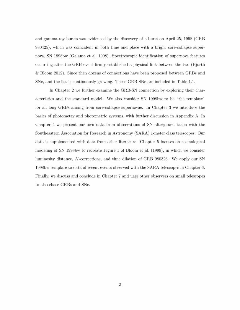
2.1 Complete light curves of SN 1998bw. Open symbols display the earlier ob-servations of Galama et al. (1998) and later observations of Sollerman et al.(2002). Solid symbols bridging the two sets are observations presented byClocchiatti et al. (2011). From Clocchiatti et al. (2011). . . . . . . . . . . . 7

2.2 Spectral evolution of GRB-SNe 1998bw (Patat et al. 2001) and 2003dh (Hjorthet al. 2003). Solid lines indicate the spectra of SN 2003dh and dotted linesindicate spectra of SN 1998bw. Times are indicated in the rest frame, daysafter the GRB. From Hjorth et al. (2003). . . . . . . . . . . . . . . . . . . 8

2.3 Montage of the main supernova types, in order to highlight the distinguishingfeatures of their spectra. These main distinguishing features are marked incolor and annotated. From Modjaz et al. (2014). . . . . . . . . . . . . . . . 10

2.4 Number of GRB-SNe at redshifts to z ≈ 1. Data from Table 1.1. . . . . . . 11

4.1 Finding chart of SN 2017iuk. The left image is an archival DSS image andthe right image is a stacked R-band image taken with SARA-CT. . . . . . . 18

4.2 R-magnitude data of GRB 171205A / SN 2017iuk. Blue x’s indicate datataken using the SARA telescopes and orange dots indicate data taken fromGCNs. Time in days indicates the time since the detection of GRB 171205A. 19

4.3 Finding chart of AT 2018cow. The left image is an archival DSS image andthe right image is a stacked R-band image taken with SARA-KP. . . . . . . 20

4.4 R-magnitude data of AT 2018cow. Blue x’s indicate data taken using theSAR-KP telescope and orange dots indicate data taken from ATels. Time indays indicates the time since the detection of the transient source. . . . . . 21

5.1 The spectrum of SN 1998bw on JD 2450946.9 (May 13, 1998). From Patatet al. (2001). . . . . . . . . . . . . . . . . . . . . . . . . . . . . . . . . . . . 25

5.2 The change in magnitude of SN 1998bw with respect to its peak magnitudeof 13.90. . . . . . . . . . . . . . . . . . . . . . . . . . . . . . . . . . . . . . . 26

5.3 The light curve of SN 1998bw redshifted to z = 0.5 (red), 1.0 (green), and 1.5(blue). Small circles indicate redshifting using the Euclidean distance andplus signs indicate redshifting using the luminosity distance. The originalmagnitudes are indicated by black stars. . . . . . . . . . . . . . . . . . . . 28

vii

5.4 The light curve of SN 1998bw redshifted and time dilated at z = 0.5 (red),1.0 (green), and 1.5 (blue). Magnitudes were calculated using luminositydistance. The original observed time scale and magnitudes are indicated byblack stars. . . . . . . . . . . . . . . . . . . . . . . . . . . . . . . . . . . . . 30

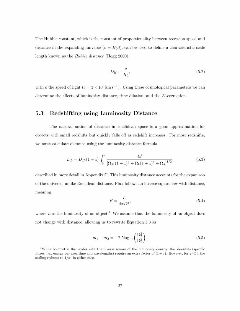
5.5 K-corrections up to redshift z = 0.85. These corrections are added to mRo =13.90 to obtain the corrected mRe . . . . . . . . . . . . . . . . . . . . . . . . 31

6.1 GRB 980326: the SN 1998bw template is shifted and time-dilated to approx-imate the redshift of GRB 980326. . . . . . . . . . . . . . . . . . . . . . . . 34

6.2 GRB 171205A / SN 2017iuk data fit with the SN 1998bw template redshiftedto z = 0.03 (red), 0.04 (green), and 0.06 (blue). The known redshift of thisburst is z = 0.037. . . . . . . . . . . . . . . . . . . . . . . . . . . . . . . . . 35

6.3 AT 2018cow data fit with the SN 1998bw template redshifted to z = 0.014,the known redshift of the event. . . . . . . . . . . . . . . . . . . . . . . . . 36

A.1 Passbands of the broad-band Johnson-Cousins UBV RI photometric system.From Bessell (2005). . . . . . . . . . . . . . . . . . . . . . . . . . . . . . . . 42

C.1 The E-function (C.1a) and the y-function (C.1b) as functions of redshift z. 45C.2 Luminosity distance and Euclidean distance to a redshift z = 3.0. . . . . . . 45

viii

Chapter 1

Introduction

Gamma-ray bursts (GRBs), first observed in the late 1960s by the Vela satellites

(Klebesadel et al. 1973), are intense flashes of electromagnetic radiation that last on the

order of seconds and have typical photon energies of several hundred keV. These bursts arrive

at Earth from unpredictable locations and can occur several times each day. Early theories

predicted that the source of GRBs was local, created within the Milky Way galaxy. However,

data from the Burst and Transient Source Experiment (BATSE) aboard the Compton

Gamma-Ray Observatory (CGRO) showed that GRBs are isotropically distributed across

the sky, thereby providing evidence that the bursts are of extragalactic origin (Fishman &

Meegan 1995).

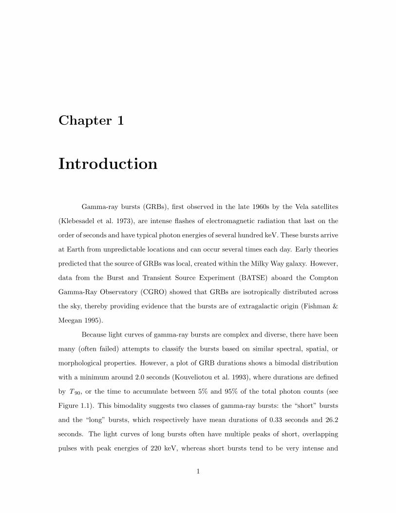
Because light curves of gamma-ray bursts are complex and diverse, there have been

many (often failed) attempts to classify the bursts based on similar spectral, spatial, or

morphological properties. However, a plot of GRB durations shows a bimodal distribution

with a minimum around 2.0 seconds (Kouveliotou et al. 1993), where durations are defined

by T 90, or the time to accumulate between 5% and 95% of the total photon counts (see

Figure 1.1). This bimodality suggests two classes of gamma-ray bursts: the “short” bursts

and the “long” bursts, which respectively have mean durations of 0.33 seconds and 26.2

seconds. The light curves of long bursts often have multiple peaks of short, overlapping

pulses with peak energies of 220 keV, whereas short bursts tend to be very intense and

1

Figure 1.1: Histogram of gamma-ray burst durations, defined by T90. The bimodality ofthe plot indicates two classes of bursts. From Kouveliotou et al. (1993).

symmetric with peak energies of 360 keV (Hakkila et al. 2000).

With the classification of long and short bursts came several various theories to

explain their progenitors. Precise and rapid localizations of short bursts indicated an asso-

ciation with regions of little or no star formation, such as elliptical galaxies (Bloom et al.

2006). This ruled out massive stars as a source of short bursts and provided support towards

the leading hypothesis that they instead originate from neutron star-neutron star mergers

or neutron star-black hole mergers (Bloom et al. 2006). Confirmation for this theory came

with the detection of short GRB 170817A only 1.7 seconds after the detection of gravita-

tional wave GW170817, a signal from the merger of two neutron stars located about 40 Mpc

away (LIGO Scientific Collaboration et al. 2017). A transient observed across the ultravio-

let, optical, and infrared wavelengths (known as a kilonova) provided further identification

of the host galaxy.

Most observed gamma-ray bursts (∼70%) are of the long type. These long GRBs

have been studied more intensively than their short counterparts. The localization of their

afterglows indicated an association with young, active star-forming galaxies and an origin

of massive star death (Woosley & Bloom 2006). The connection between supernovae (SNe)

2

and gamma-ray bursts was evidenced by the discovery of a burst on April 25, 1998 (GRB

980425), which was coincident in both time and place with a bright core-collapse super-

nova, SN 1998bw (Galama et al. 1998). Spectroscopic identification of supernova features

occurring after the GRB event firmly established a physical link between the two (Hjorth

& Bloom 2012). Since then dozens of connections have been proposed between GRBs and

SNe, and the list is continuously growing. These GRB-SNe are included in Table 1.1.

In Chapter 2 we further examine the GRB-SN connection by exploring their char-

acteristics and the standard model. We also consider SN 1998bw to be “the template”

for all long GRBs arising from core-collapse supernovae. In Chapter 3 we introduce the

basics of photometry and photometric systems, with further discussion in Appendix A. In

Chapter 4 we present our own data from observations of SN afterglows, taken with the

Southeastern Association for Research in Astronomy (SARA) 1-meter class telescopes. Our

data is supplemented with data from other literature. Chapter 5 focuses on cosmological

modeling of SN 1998bw to recreate Figure 1 of Bloom et al. (1999), in which we consider

luminosity distance, K-corrections, and time dilation of GRB 980326. We apply our SN

1998bw template to data of recent events observed with the SARA telescopes in Chapter 6.

Finally, we discuss and conclude in Chapter 7 and urge other observers on small telescopes

to also chase GRBs and SNe.

3

GRB SN z T90 (s) mpeak Reference

920613 1992ae 0.075 129.4 18.47V IAUC5554951107 1995bc 0.048 43.52 18.5V IAUC6275970514 1997cy 0.063 1.3 16.8 IAUC6706980425 1998bw 0.0085 18 13.6 IAUC6895991002 1999eb 0.018 1.9 16.2 IAUC7268011121 2001ke 0.362 47 23.0 IAUC7857020211 2002lt 1.006 2.80 24.5 IAUC8197030329 2003dh 0.1685 22.76 16.2 IAUC8114031203 2003lw 0.1055 37.0 20.5 IAUC8308

050525A 2005nc 0.606 8.84 24.0 IAUC8696060218 2006aj 0.0334 2100 17.3 IAUC8674081007 2008hw 0.53 9.01 16.4 CBET1602091127 2009nz 0.49 7.42 21.6 CBET2288

100316D 2010bh 0.0591 1300 20.0 CBET2227101219B 2010ma 0.552 51 17.8 CBET2706111209A 2011kl 0.67702 10000 20.0 CBET4196120422A 2012bz 0.2383 5.35 20.6 CBET3100120714B 2012eb 0.3984 159 18.6 CBET3200130215A 2013ez 0.597 40 14.2 CBET3637130427A 2013cq 0.3399 162.8 12.0 CBET3531130702A 2013dx 0.145 59 17.4 CBET3587130831A 2013fu 0.4791 32.5 14.1 CBET3677161219B 2016jca 0.1475 6.94 19.0 GCN20308171010A 2017htp 0.328 70.3 21.8 GCN21985171205A 2017iuk 0.037 189.4 16.0 GCN22177

Table 1.1: Gamma-ray bursts with associated supernovae. Magnitudes are reported for theR band unless noted by a subscript. Data from Guessoum et al. (2017), Hjorth & Bloom(2012), Modjaz et al. (2016).

4

Chapter 2

The GRB-SN Connection

Colgate (1968) first proposed a model of gamma-ray bursts before the phenomenon

had even been discovered, associating them with the breakout of shocks from the surfaces

of supernovae. However, the discoverers of such gamma-ray emissions found no evidence for

the predicted connection with SNe (Klebesadel et al. 1973). For over two decades, thousands

of GRBs and hundreds of SNe were localized and yet no connection was established. By

1997, the search for GRB counterparts came to fruition with the first rapidly available

and accurate GRB error boxes, produced by the two Wide Field Cameras (WFC) on the

BeppoSAX satellite (Boella et al. 1997). Follow-ups of bursts eventually pointed towards a

cosmological origin, occurring in regions of active star formation. Paczynski (1986) predicted

that these “gamma-ray bursters” would release 1051 ergs within 1 second, making them

comparable to the kinetic energy released by a supernova. As redshifts of GRBs were

determined and geometric corrections made to account for beaming, the total energy release

in γ-rays was found to be around 1051 ergs, as had been hypothesized (e.g. Kumar & Piran

(2000)).

Despite this similarity in energy between GRBs and SNe, the phenomena were

considered unrelated. The event that clicked the connection into place was the discovery of

GRB 980425, which occurred on April 25, 1998. This underluminous GRB was coincident

in time (within a few days) and location (within a few arcminutes) with SN 1998bw, an

5

unusually bright supernova (EK = 1052 ergs; Galama et al. (1998)) located in the late-type

galaxy ESO184-G82 at a redshift z = 0.0085 (Tinney et al. 1998). Although the connection

was initially doubted by some, X-ray data confirmed the association of the GRB with the

supernova (Pian et al. 2000). Spectroscopic analysis of SN 1998bw revealed a lack of H

and He absorption lines with a weak Si II absorption line, suggesting a classification of a

Type Ic broad-line supernova (Patat & Piemonte 1998). However, at such a low redshift,

the energy emitted in gamma-rays was calculated to be Eγ = 8.5 ± 0.1 × 1047 ergs, over

three orders of magnitude fainter than what is expected of long-duration bursts (Woosley

& Bloom 2006). In addition, no optical afterglow was detected, as is common in most other

GRBs (see Section 2.1). These three factors caused some (e.g., Kulkarni et al. (1998)) to

point towards a different class of GRB than the “truly cosmological GRB”, defined by a

significant redshift, high energy output, and an afterglow decaying as a power-law (Hjorth

& Bloom 2012).

Nevertheless, SN 1998bw was thoroughly observed and its light curve was the subject

of many extensive studies (e.g. Clocchiatti et al. (2011), Patat et al. (2001), Sollerman et al.

(2002)). With spectral and photometric data readily available (see Figure 2.1), SN 1998bw

is often used as a template to constrain other supernova light curves. For a typical GRB-

SN, the three components of measured flux are the afterglow (AG), the supernova, and

the host galaxy’s constant source. In order for the SN component to be analyzed, it must

first be decomposed from the optical light curve. The late-time “supernova bump” is then

compared to a template supernova, namely SN 1998bw. This approach has been used in

many studies (e.g. Cano et al. (2014), Cano et al. (2017), Zeh et al. (2004)), pointing

towards SN 1998bw as “the template” for all GRB-SNe.

Almost five years later, on March 29, 2003, any doubts were eliminated concern-

ing the connection between gamma-ray bursts and supernovae with the detection of GRB

030329 in accordance with SN 2003dh. At a redshift of z = 0.1685 (Greiner et al. 2003),

the burst was considered truly cosmological and, unlike GRB 980425, was followed by a

very bright afterglow (R ∼ 13; Price & Peterson (2003)). The optical spectrum of the burst

6

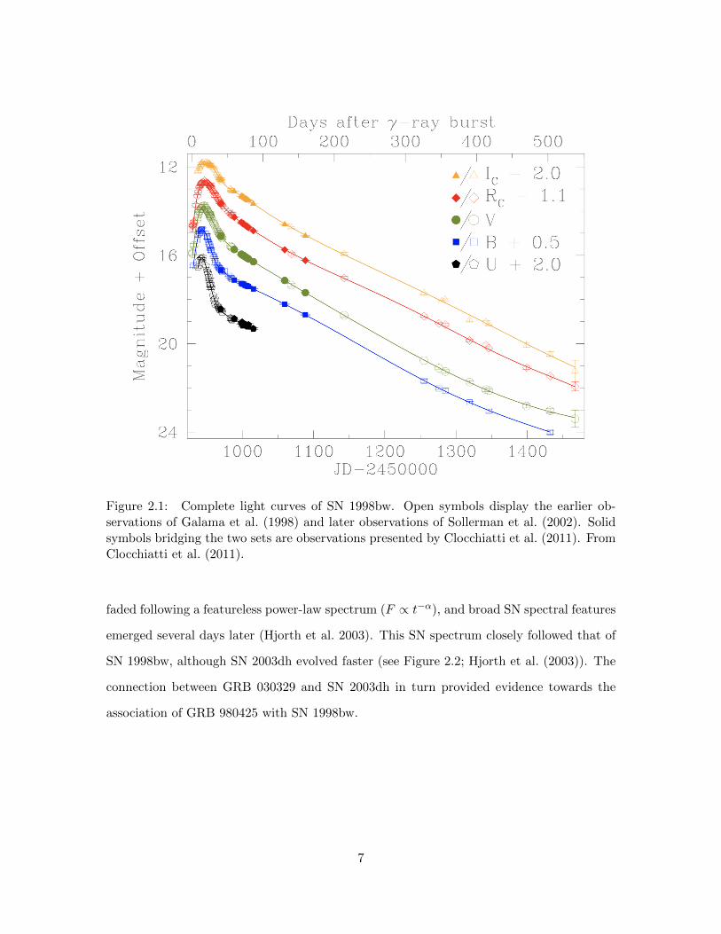
Figure 2.1: Complete light curves of SN 1998bw. Open symbols display the earlier ob-servations of Galama et al. (1998) and later observations of Sollerman et al. (2002). Solidsymbols bridging the two sets are observations presented by Clocchiatti et al. (2011). FromClocchiatti et al. (2011).

faded following a featureless power-law spectrum (F ∝ t−α), and broad SN spectral features

emerged several days later (Hjorth et al. 2003). This SN spectrum closely followed that of

SN 1998bw, although SN 2003dh evolved faster (see Figure 2.2; Hjorth et al. (2003)). The

connection between GRB 030329 and SN 2003dh in turn provided evidence towards the

association of GRB 980425 with SN 1998bw.

7

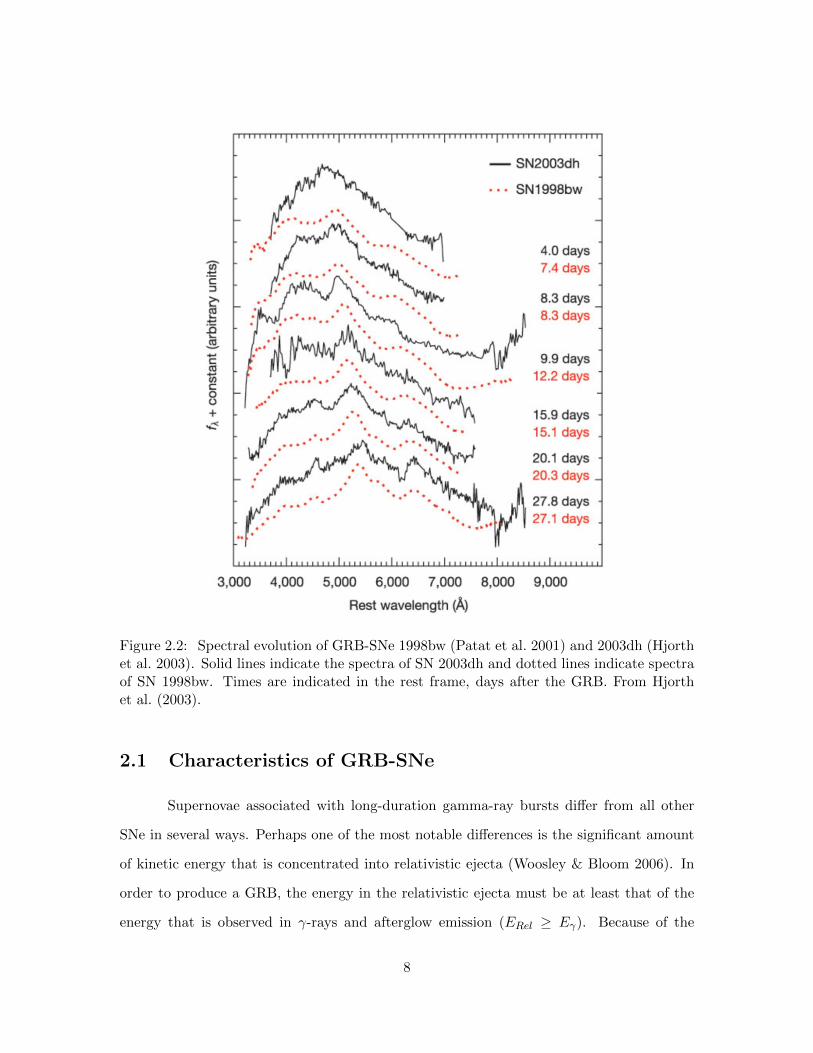
Figure 2.2: Spectral evolution of GRB-SNe 1998bw (Patat et al. 2001) and 2003dh (Hjorthet al. 2003). Solid lines indicate the spectra of SN 2003dh and dotted lines indicate spectraof SN 1998bw. Times are indicated in the rest frame, days after the GRB. From Hjorthet al. (2003).

2.1 Characteristics of GRB-SNe

Supernovae associated with long-duration gamma-ray bursts differ from all other

SNe in several ways. Perhaps one of the most notable differences is the significant amount

of kinetic energy that is concentrated into relativistic ejecta (Woosley & Bloom 2006). In

order to produce a GRB, the energy in the relativistic ejecta must be at least that of the

energy that is observed in γ-rays and afterglow emission (ERel ≥ Eγ). Because of the

8

effects of beaming, the value of Eγ can be difficult to measure directly but is estimated to

be around 1051 ergs (Bloom et al. 2003). ERel, inferred from late-time radio observations,

is measured to be ∼ 5× 1051 ergs.

GRB-SNe are most likely Type Ic-BL SNe, based on the spectroscopic data of various

GRB-SNe. These supernovae have an absence of hydrogen in their spectra, placing them in

the Type I classification. Sufficient spectra observations also indicate an absence of neutral

helium (He I) and weak or absent absorption lines of singly-ionized silicon (Si II), leading to

a Type Ic classification. Broad-line (BL) features are also apparent in the spectra of GRB-

SNe; these features are due to high velocities, such as the Si II line width of SN 1998bw that

suggested expansion speeds of 30,000 km s−1 (Patat et al. 2001). The differences in spectral

features of various types of supernovae are shown in Figure 2.3 (Modjaz et al. 2014).

Because of the brightness of GRB-SNe, theory demands a high production of 56Ni to

power the luminosity for long timescales (weeks to months). The combination of high mass,

high velocity, and high 56Ni mass implies a kinetic energy of ESN ∼ 1052 ergs (Woosley &

Bloom 2006). In order for the iron core to collapse into a neutron star or black hole, energy

must be released on the order of Eν ∼ 1053 ergs. From this explosion, 99% is carried by

neutrinos, 1% goes into kinetic energy of the expanding ejecta, and 0.01% goes into light;

the energy of the ejecta is then EK ∼ 1051 ergs (Hartmann 2010).

As the most energetic explosions in the universe, it may seem surprising that a

connection between GRBs and SNe took several years to establish. However, the rate for

GRB-SNe is not as frequent as one may expect. The supernova rate is estimated as 1

SN/100 yrs/1 Milky Way-type galaxy or ∼ 0.5 Gpc−3 yr−1 (Schmidt 2001). An estimated

15 − 20% of all SNe are observed to be of Type Ib/c, or ∼ 4.8 × 104 Gpc−3 yr−1 (Marzke

et al. 1998). Of all Type Ib/c SNe, about 5− 10% are classified as SN Ic-BL; this indicates

a rate of about 10−6 − 10−5 per year. At the 90% confidence level, less than 10% of all SN

Ib/c have an off-axis GRB (Soderberg et al. 2006).

The data thus indicate that most long GRBs do not have a detected associated

supernova. Regardless, some favor the hypothesis that all long-duration GRBs lead to

9

Figure 2.3: Montage of the main supernova types, in order to highlight the distinguish-ing features of their spectra. These main distinguishing features are marked in color andannotated. From Modjaz et al. (2014).

supernovae (e.g. Bloom et al. (2003)) and extrinsic biases result in a decreased probability

of detecting a supernova. We note that many of the connected GRB-SN events occur within

redshift z < 0.5 (see Figure 2.4), most likely due to the biases briefly listed here (Woosley

& Bloom 2006):

1. Localization - Poor localization of bursts impede the ability of telescopes to discover

emerging supernovae.

2. Dust - The sensitivity of SN observations may be diminished, particularly for those

that occur near the line-of-sight through the galaxy.

10

Figure 2.4: Number of GRB-SNe at redshifts to z ≈ 1. Data from Table 1.1.

3. Redshift and luminosity distance - Higher redshifts (z ≈ 0.5) imply high K-corrections

and higher distance modulus and a greater suppression of emissivity, making Type

Ib/c SNe more difficult to detect.

4. Host galaxies - The host galaxies of GRBs may contaminate the light of SN such that

resolving out diffuse host light may become impossible.

2.2 The Collapsar Model

Various models of ordinary core-collapse supernovae have been explored in the liter-

ature (e.g. see sources contained within Woosley & Bloom (2006)). The “standard model”

of the collapsar (e.g. MacFayden et al. (2001)) begins with a main-sequence massive star

(M > 30M). At T ∼ 1010 K and ρ ∼ 1010 g cm−3, the iron core of the star collapses, trig-

gered by electron capture and photodisintegration. A rebound launches a shock wave but

11

quickly loses velocity due to neutrino loss. Much of the ejected mass falls back onto the core

remnant at a rate of 0.1−0.3M/s, producing a black hole or a “proto-neutron star”. If the

star is rotating quickly enough, the gravitational potential energy of the infalling material

drives a pair of relativistic jets out along the rotational axis. These jets transfer enough

energy into the ejected shell that a superluminous supernova can be observed. Gamma-rays

are geometrically beamed outwards by the jets to angles of ∼ 5(∼ 0.1 rad), meaning that

observers will not detect the jets if they are outside the viewing angle. Supernovae, on the

contrary, emit isotropically and therefore can be viewed from any angle.

With this collapsar model comes a few constraints (Woosley & Heger 2006). First,

the star undergoing core-collapse must be massive enough to produce a neutron star or a

black hole with enough explosion energy to expel the outer layers of the star; this places a

lower limit of around 10 M. If the star is too massive, however, a black hole may form

before an outgoing shock is launched. Second, the star must be rapidly rotating in order

to develop an accretion torus and drive the jets outwards after collapse; too little rotation

will fail to create a gamma-ray burst. Third, the star must have low metallicity and must

lose its hydrogen envelope prior to collapse. Stars with low metallicity tend to have a lower

mass loss rate; too much mass loss makes the star too light to explode into a black hole

(Woosley & Bloom 2006).

12

Chapter 3

Photometric Observations of

Afterglows

In order to observe the evolution of gamma-ray bursts and supernovae, photometric

measurements must be taken. Photometry, derived from the Greek photos (“light”) and

metron (“measure”), is the measure of flux of an object’s electromagnetic radiation (Sterken

& Manfroid 1992). For astronomical purposes a charged-coupled device (CCD) is often

used to observe and record these signals in terms of counts and convert the counts into

instrumental magnitudes. The instrumental magnitudes are compared to known magnitudes

of other objects, such as standard stars, in order to determine the magnitudes of the observed

objects. In this chapter we present a brief overview of photometry, as the topic is rather

extensive and can fill entire books (e.g. Sterken & Manfroid (1992); Kitchin (1998); Howell

(2000)). More in-depth information is described in Appendix A.

3.1 Basics of Photometry

To begin photometry, the proper calibration images–bias frames, dark frames, and

flat frames–must be taken and correctly applied to the data images, which consist of both the

object frames and the frames containing a set of Landolt standard stars. The magnitudes of

13

these standard stars (Landolt 1992) have been thoroughly studied and measured, allowing

them to be used as a comparison for the magnitudes of other celestial objects. This method

of comparing instrumental magnitudes to stars of known magnitudes is known as relative

photometry. The Landolt standard stars are centered around the celestial equator so they

can be observed from either hemisphere; they are also non-variable, not too bright as to

saturate detectors (11.5 ≤ M ≤ 16.0), and individual sets are close together and cover a

wide color range (−0.3 to +2.3).

After the data images have been reduced, photometric measurements can be made.

Image processing programs such as IRAF (Interactive Reduction and Analysis Facility), IDL

(Interactive Data Language), or ESO-MIDAS (European Southern Observatory - Munich

Image Data Analysis System) are used to convert the count rates measured by the CCD

into instrumental magnitudes. After atmospheric extinction corrections and comparisons

to standard stars, these instrumental magnitudes are converted into magnitudes that can

be placed on a standard physical flux scale. In this study we used IRAF to reduce our data

and take photometric measurements.

3.2 Photometric Systems

The total luminosity of an object, integrated over all wavelengths, is known as its

bolometric luminosity. However, observing celestial objects over all wavelengths is often not

necessary or even possible. Filters are often used to pass through only certain wavelengths

of light. Various photometric systems, which are defined by a list of standard magnitudes

and colors measured at specific bandpasses, are used to determine the magnitudes of ob-

jects (Bessell 2005). These systems have a known sensitivity to incident radiation and are

characterized according to the widths of their passbands. For example, broad band systems

have passbands wider than 400 A, such as the Johnson-Cousins UBV RI system that is

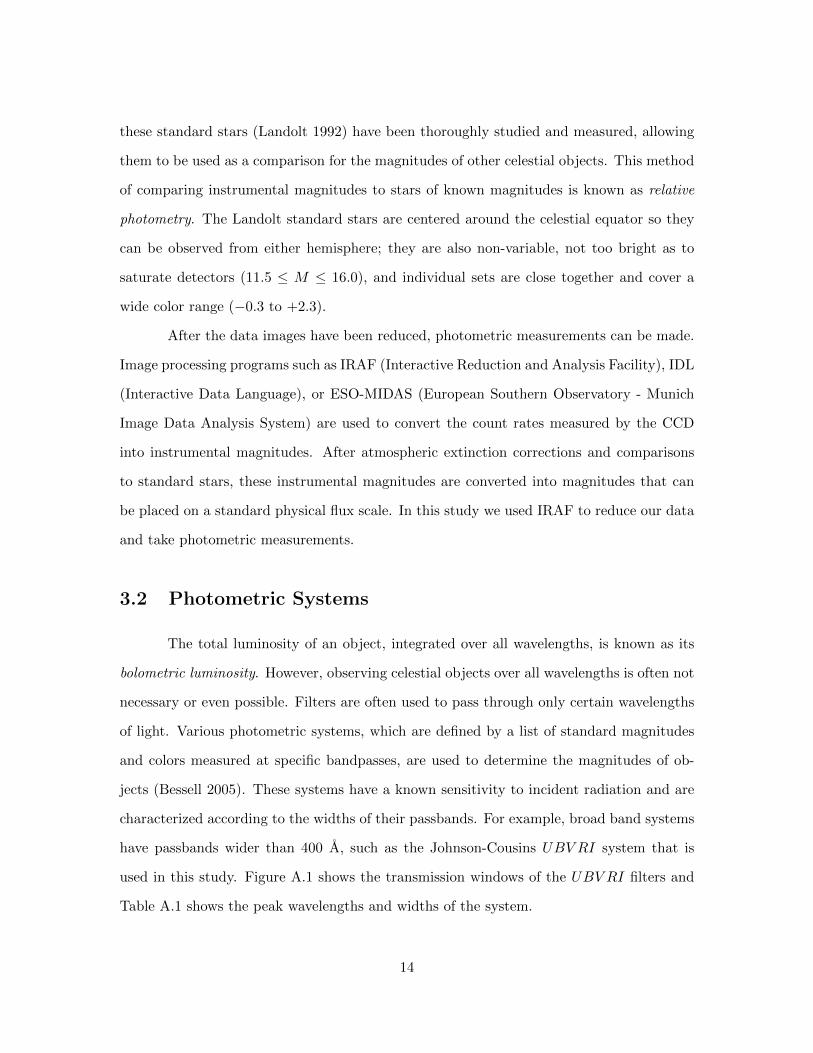
used in this study. Figure A.1 shows the transmission windows of the UBV RI filters and

Table A.1 shows the peak wavelengths and widths of the system.

14

In general, an object such as a star has a different magnitude depending on the filter

used to observe it. The magnitude of an object is defined as

mR = −2.5log10(FR) + ZP, (3.1)

where the subscript R indicates that the object was observed through the R passband. The

added constant ZP sets the zero-point of the magnitude scale in use. The STMag system

uses the flux density of Vega at the effective wavelength of the Johnson V band (∼ 5500 A)

to set the zero point (Phillips 2008), leading to the relation

mλ = −2.5log10(Fλ)− 21.1. (3.2)

This indicates that we can determine a star’s magnitude if we know its flux at a certain

wavelength. If two stars are observed through the same filter, the difference between their

magnitudes can be determined using the relation

m1 −m2 = −2.5log10(F1/F2), (3.3)

where F1 and F2 are the fluxes of each star. In addition to the passband used, observed

light from an object can be diminished by Earth’s atmosphere. A star at the zenith will

suffer the least from atmospheric extinction, whereas a star closer to the horizon will suffer

the most, as the path length through the atmosphere is longer (Bessell 2005). This path

length is called the airmass, approximated by sec(Z) such that the airmass is 1 at zenith.

Both the airmass and the passband used must be taken into consideration when determining

photometric values.

Even after considering the filter, airmass, and exposure time (among many other

variables), observers are nevertheless limited by the upper limits of the telescope used.

Small telescopes, often around 1 meter in diameter, are only able to detect objects up to

∼20th magnitude. Larger telescopes, such as the 10-m Keck Telescope, have an upper limit

15

of almost 26th magnitude (Keck Observatory 2016). Even more advantageous, telescopes

above the Earth’s atmosphere avoid sky brightness and can see even deeper objects; the

James Webb Space Telescope (JWST) is expected to have an upper limit of 34th magnitude

(Mather 2017). Knowing the upper limit of a telescope allows observers to smartly choose

targets for photometric or spectroscopic studies.

16

Chapter 4

Observations with SARA

The Southeastern Association for Research in Astronomy (SARA) is a consortium

consisting of over ten southeastern colleges and universities with small astronomy depart-

ments (Keel et al. 2016). Members include Clemson University, University of Alabama,

Florida Gulf Coast University, and Butler University, among others. The consortium op-

erates three telescopes in various locations: the 0.96 m telescope at Kitt Peak, Arizona

(SARA-KP), a 0.6 m aperture on Cerro Tololo, Chile (SARA-CT), and the 1.0 m Jacobus

Kapteyn Telescope at the Roque de los Muchachos, La Palma, Spain (SARA-RM). Each

telescope has a CCD system and is controlled remotely.

Use of all three SARA telescopes has been vital to this study for observing gamma-

ray burst afterglows and supernovae. Some of the data has been supplemented with data

from the Gamma-ray Coordinates Network (GCN) and/or The Astronomer’s Telegram

(ATel). We report our observational data for several events in the following sections.

4.1 GRB 171205A / SN 2017iuk

Swift detected a burst at 07:20:43 UT on December 5, 2017 located at a right as-

cension of 11:09:47 and a declination of -12:36:12 (D’Elia et al. 2017). The XRT position

contained the spiral galaxy 2MASX J11093966-1235116, located at z = 0.037 (Izzo et al.

17

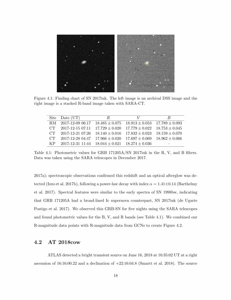
Figure 4.1: Finding chart of SN 2017iuk. The left image is an archival DSS image and theright image is a stacked R-band image taken with SARA-CT.

Site Date (UT) R V B

RM 2017-12-09 06:17 18.485± 0.075 18.913± 0.053 17.789± 0.093CT 2017-12-15 07:11 17.729± 0.020 17.779± 0.022 18.753± 0.045CT 2017-12-21 07:26 18.140± 0.016 17.832± 0.023 19.159± 0.070CT 2017-12-28 04:47 17.966± 0.020 17.697± 0.069 18.962± 0.066KP 2017-12-31 11:44 18.044± 0.021 18.274± 0.036 –

Table 4.1: Photometric values for GRB 171205A/SN 2017iuk in the R, V, and B filters.Data was taken using the SARA telescopes in December 2017.

2017a); spectroscopic observations confirmed this redshift and an optical afterglow was de-

tected (Izzo et al. 2017b), following a power-law decay with index α = 1.41±0.14 (Barthelmy

et al. 2017). Spectral features were similar to the early spectra of SN 1998bw, indicating

that GRB 171205A had a broad-lined Ic supernova counterpart, SN 2017iuk (de Ugarte

Postigo et al. 2017). We observed this GRB-SN for five nights using the SARA telescopes

and found photometric values for the B, V, and R bands (see Table 4.1). We combined our

R-magnitude data points with R-magnitude data from GCNs to create Figure 4.2.

4.2 AT 2018cow

ATLAS detected a bright transient source on June 16, 2018 at 10:35:02 UT at a right

ascension of 16:16:00.22 and a declination of +22:16:04.8 (Smartt et al. 2018). The source

18

Figure 4.2: R-magnitude data of GRB 171205A / SN 2017iuk. Blue x’s indicate data takenusing the SARA telescopes and orange dots indicate data taken from GCNs. Time in daysindicates the time since the detection of GRB 171205A.

is spatially coincident with the galaxy CGCC 137-068, which is at a redshift z = 0.014145,

and was thought to be a cataclysmic variable, a bright supernova, or something else. The

host galaxy has a magnitude of 15.7 (Zwicky & Herzog 1963). Spectroscopy of the transient

revealed a mostly featureless spectrum and a weak broad-lined feature at ∼ 5040 A, similar

to a feature found in Ic-BL SN spectra (Rivera Sandoval & Maccarone 2018); this led

some observers to believe that the “orphan afterglow” may be the supernova counterpart

to an off-axis GRB. We observed this transient for four nights using the SARA-KP and

SARA-RM telescopes and found photometric values for the R band (see Table 4.2). We

combined our R-magnitude data with R-magnitude data from ATels to create Figure 4.4;

we also include a magnitude taken on SARA-RM by a fellow member of the consortium,

Bill Keel of University of Alabama. However, we note that our magnitudes on 2018-06-21

and 2018-06-22 are about half a magnitude brighter than those announced in Astronomer’s

19

Figure 4.3: Finding chart of AT 2018cow. The left image is an archival DSS image and theright image is a stacked R-band image taken with SARA-KP.

Site Date (UT) R

KP 2018-06-20 05:28 14.266± 0.010KP 2018-06-21 03:50 14.035± 0.007KP 2018-06-22 03:37 14.170± 0.014RM 2018-07-06 01:06 15.030± 0.010RM 2018-07-17 21:36 15.473± 0.019

Table 4.2: Photometric values for AT 2018cow in the R filter. Data was taken using theSARA-KP and SARA-RM telescopes in June and July 2018.

Telegrams; this could be due to photometric techniques that did not completely subtract

the background light of the host galaxy.

4.3 Other Observations

As described in Chapter 2, not all gamma-ray bursts appear to have an associated

supernova. Some supernovae are also too faint to observe using the SARA telescopes due

to their upper limits of ∼20th magnitude. In this section, we present data for two bursts

that we observed but had no associated supernovae.

4.3.1 GRB 180514

Swift detected a burst on May 14, 2018 at 13:25:33 UT with a right ascension of

13:09:36 and a declination of +36:58:10 (LaPorte et al. 2018). Follow-up observations could

20

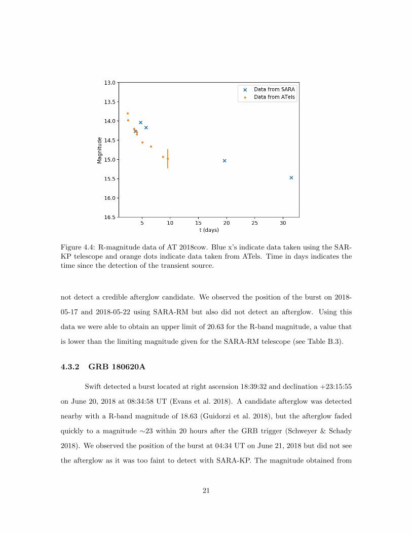
Figure 4.4: R-magnitude data of AT 2018cow. Blue x’s indicate data taken using the SAR-KP telescope and orange dots indicate data taken from ATels. Time in days indicates thetime since the detection of the transient source.

not detect a credible afterglow candidate. We observed the position of the burst on 2018-

05-17 and 2018-05-22 using SARA-RM but also did not detect an afterglow. Using this

data we were able to obtain an upper limit of 20.63 for the R-band magnitude, a value that

is lower than the limiting magnitude given for the SARA-RM telescope (see Table B.3).

4.3.2 GRB 180620A

Swift detected a burst located at right ascension 18:39:32 and declination +23:15:55

on June 20, 2018 at 08:34:58 UT (Evans et al. 2018). A candidate afterglow was detected

nearby with a R-band magnitude of 18.63 (Guidorzi et al. 2018), but the afterglow faded

quickly to a magnitude ∼23 within 20 hours after the GRB trigger (Schweyer & Schady

2018). We observed the position of the burst at 04:34 UT on June 21, 2018 but did not see

the afterglow as it was too faint to detect with SARA-KP. The magnitude obtained from

21

photometry of a star located close to the burst is similar to the magnitude that is given by

the USNO-A2.0 catalogue; we obtained a magnitude of 16.92 ± 0.03 whereas the accepted

magnitude is 16.40 (Monet et al. 1997).

22

Chapter 5

Cosmological Modeling

Because SN 1998bw was a close, bright supernova, it was thoroughly observed and

analyzed. Although GRB 980425 did not have an optical afterglow, this GRB-SN can be

used as a template for other GRB-SNe. Oftentimes the distance to a supernova is unknown

because of a lack of spectroscopic observations; using the light curve of SN 1998bw as a

template can provide constraints on supernova distance as well as a predicted peak time

and duration. The template need only be translated and stretched to match the light curves

of other supernovae in question.

For example, GRB 980326 was detected on March 26, 1998 by BeppoSAX and an

optical afterglow was identified (Groot et al. 1998). A power-law decay is apparent in

the light curve as is a subsequent rebrightening phase (Bloom et al. 1999), but a redshift

was never determined for the burst. Nine months after the GRB event, no host galaxy

was detected at the position of the optical transient, indicating a very faint host galaxy.

Bloom et al. (1999) analyzed the light curve of the afterglow of GRB 980326 by overlaying a

template of the SN 1998bw light curve at different redshifts. They found that the “GRB +

supernova” model best fit the data at a redshift of z ≈ 1 and that the rebrightening phase

of the light curve was adequately described by a “supernova bump”.

In this chapter and the next, we recreate Figure 1 from Bloom et al. (1999) by

applying various cosmological parameters and distances to SN 1998bw data to fit a template

23

to GRB 980326 data. We describe our application of luminosity distance, the K−correction,

and time dilation here. Basic concepts of cosmology are briefly explained in Appendix C,

as the topic is very extensive and is often covered in a semester’s worth of graduate classes

(Ryden 2003).

5.1 The SN 1998bw Template

We used data of SN 1998bw to create our template (Galama et al. (1998), Patat et al.

(2001)). The R-magnitude of SN 1998bw peaked on May 13.4, 1998 (JD 2450946.9), about

17 days after the detection of GRB 980425 (Galama et al. 1998). We used the spectrum

from this day (Patat et al. 2001) as a standard spectrum for all later measurements (Figure

5.1). The flux at the central wavelength for the R filter (6407 A; Bessell (2005)) was

Fλ = 1.003827× 10−14 erg s−1 cm−2 A−1

. We converted this to a magnitude using Equation

3.2 to find the peak R magnitude of 13.90. We held this spectrum constant in time and

defined 13.90 as our “zero point”. Using the photometric data of Galama et al. (1998),

we determined the changes in magnitudes for the rise and decay of the supernova (Figure

5.2). The fit to the changes in magnitudes is used as the template for the redshifting of SN

1998bw.

5.2 Cosmological Parameters

We use a ΛCDM cosmological model and assume a flat universe such that k =

0. Using cosmological parameters from Planck Collaboration et al. (2015) we define the

Hubble constant as H0 = 67.74 ± 0.46 km s−1 Mpc−1, the matter density parameter as

ΩM = 0.308 ± 0.012, and the dark energy density parameter as ΩΛ = 0.6911 ± 0.0062

(taking the curvature density parameter as Ωk = 0). The density parameters are related

such that

ΩM + ΩΛ + Ωk = 1. (5.1)

24

Figure 5.1: The spectrum of SN 1998bw on JD 2450946.9 (May 13, 1998). From Patat et al.(2001).

25

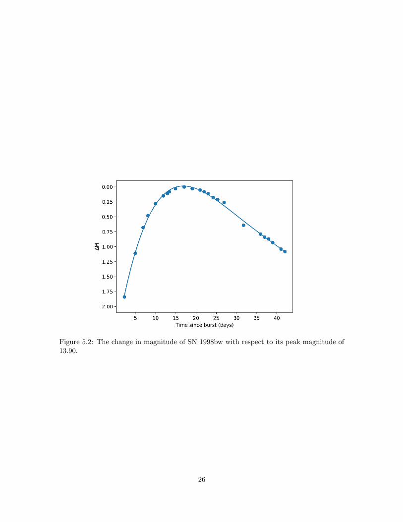
Figure 5.2: The change in magnitude of SN 1998bw with respect to its peak magnitude of13.90.

26

The Hubble constant, which is the constant of proportionality between recession speed and

distance in the expanding universe (v = H0d), can be used to define a characteristic scale

length known as the Hubble distance (Hogg 2000):

DH ≡c

H0, (5.2)

with c the speed of light (c = 3× 105 km s−1). Using these cosmological parameters we can

determine the effects of luminosity distance, time dilation, and the K-correction.

5.3 Redshifting using Luminosity Distance

The natural notion of distance in Euclidean space is a good approximation for

objects with small redshifts but quickly falls off as redshift increases. For most redshifts,

we must calculate distance using the luminosity distance formula,

DL = DH (1 + z)

∫ z

0

dz′

[ΩM (1 + z)3 + Ωk(1 + z)2 + ΩΛ]1/2, (5.3)

described in more detail in Appendix C. This luminosity distance accounts for the expanison

of the universe, unlike Euclidean distance. Flux follows an inverse-square law with distance,

meaning

F =L

4πD2, (5.4)

where L is the luminosity of an object.1 We assume that the luminosity of an object does

not change with distance, allowing us to rewrite Equation 3.3 as

m1 −m2 = −2.5log10

(D2

2

D21

). (5.5)

1While bolometric flux scales with the inverse square of the luminosity density, flux densities (specificfluxes; i.e., energy per area time and wavelengths) require an extra factor of (1 + z). However, for z 1 thescaling reduces to 1/z2 in either case.

27

Figure 5.3: The light curve of SN 1998bw redshifted to z = 0.5 (red), 1.0 (green), and1.5 (blue). Small circles indicate redshifting using the Euclidean distance and plus signsindicate redshifting using the luminosity distance. The original magnitudes are indicatedby black stars.

Using Equations 5.3 and 5.5 we can shift SN 1998bw from its original redshift z = 0.0085

to larger redshifts tested by Bloom et al. (1999), e.g. z = 0.5, 1.0, and 1.5. These shifts

and corresponding new magnitudes are shown in Figure 5.3.

5.4 Adjusting Timescales using Time Dilation

Expansion of the universe causes cosmological time dilation, meaning that observed

light was emitted by the source at an earlier time. These times are related by a factor of

28

1 + z such that

trest =tobs

(1 + z). (5.6)

For example, we observe that the R-band peak of GRB 980425 occurred at tobs = 17.04

days. In the rest frame of the supernova, this peak actually occurred at

trest =17.04 days

1 + 0.0085= 16.90 days.

If SN 1998bw occurred at a redshift z = 0.5, then we would have seen the peak at

t′obs = trest(1 + z) = (16.90 days)(1 + 0.5) = 25.34 days.

We consider time dilation effects on SN 1998bw redshifted to z = 0.5, 1.0, and 1.5

by first transforming into its rest frame to find trest and then transforming into the other

“observed” frames. Figure 5.4 shows the new magnitudes (based on luminosity distance)

and time scales of SN 1998bw.

5.5 The K-Correction

The K-correction corrects an object’s magnitude (or flux) by converting a measure-

ment from the object at redshift z into an equivalent rest-frame measurement. A photon

observed with wavelength λo was emitted by the source with wavelength λe. Like the

concept of time dilation, the two wavelengths are related by a factor of 1 + z:

λe =λo

1 + z. (5.7)

We account for the K-correction by considering only this relation (a simplification of the

more complicated transformation equation).

As stated in Section 5.1, the central wavelength for the R band is λeff = 6407 A,

which corresponds to a flux of Fλ = 1.003827× 10−14 erg s−1 cm−2 A−1

in the “fixed” spec-

29

Figure 5.4: The light curve of SN 1998bw redshifted and time dilated at z = 0.5 (red), 1.0(green), and 1.5 (blue). Magnitudes were calculated using luminosity distance. The originalobserved time scale and magnitudes are indicated by black stars.

trum of SN 1998bw. The photons we observe at 6407 A were emitted at a wavelength

λe =6407 A

1 + 0.0085= 6353 A

in the rest frame of the supernova. This wavelength corresponds to a flux of Fλ = 1.044349×

10−14 erg s−1 cm−2 A−1

, or a magnitude of mR = 13.85. The K-correction is then

K = mRe −mRo = 13.85− 13.90 = 0.05.

Using the fixed spectrum of SN 1998bw (Figure 5.1), we calculated the K-corrections for

30

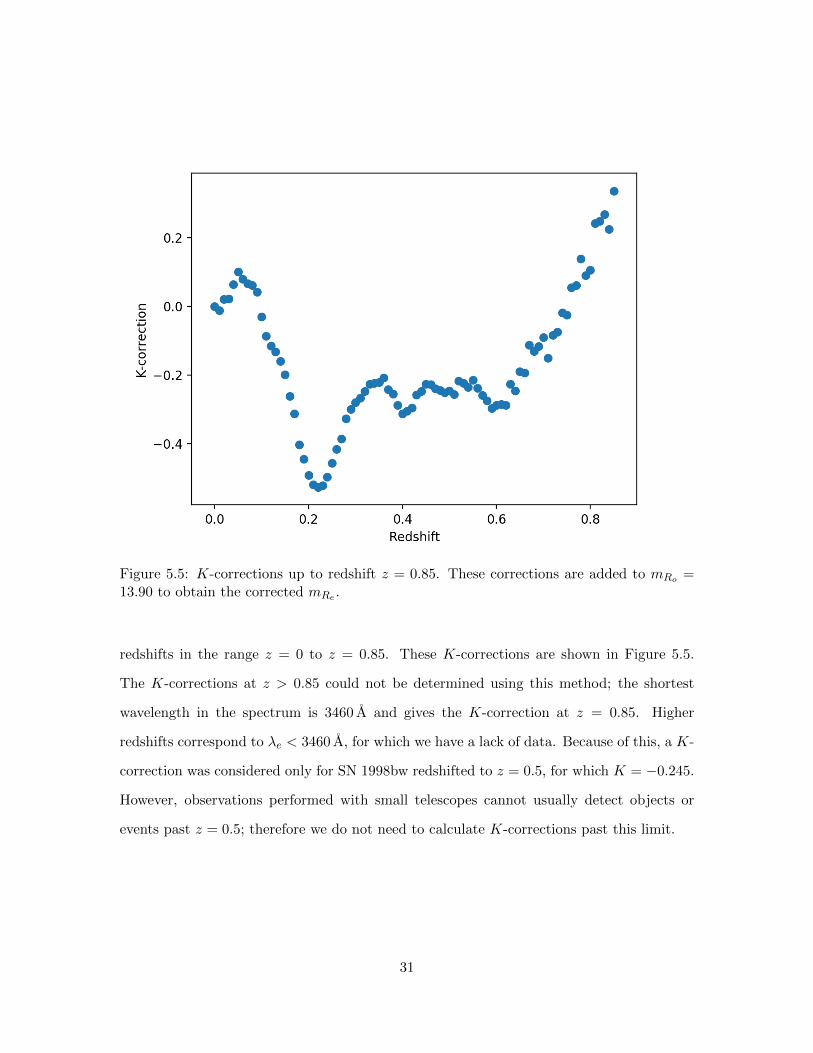
Figure 5.5: K-corrections up to redshift z = 0.85. These corrections are added to mRo =13.90 to obtain the corrected mRe .

redshifts in the range z = 0 to z = 0.85. These K-corrections are shown in Figure 5.5.

The K-corrections at z > 0.85 could not be determined using this method; the shortest

wavelength in the spectrum is 3460 A and gives the K-correction at z = 0.85. Higher

redshifts correspond to λe < 3460 A, for which we have a lack of data. Because of this, a K-

correction was considered only for SN 1998bw redshifted to z = 0.5, for which K = −0.245.

However, observations performed with small telescopes cannot usually detect objects or

events past z = 0.5; therefore we do not need to calculate K-corrections past this limit.

31

Chapter 6

Applying the SN 1998bw Template

After considering luminosity distance, time-dilation, and the K-correction, we con-

structed a template of the SN 1998bw light curve. We applied this to GRB 980326 data

to recreate Figure 1 of Bloom et al. (1999), as well as fitting data of SN 2017iuk and AT

2018cow.

6.1 Recreating the Bloom et al. (1999) Plot

We used GRB 980326 data from both Bloom et al. (1999) and Groot et al. (1998);

these dates and magnitudes are included in Table 6.1. The optical transient exhibited a

temporal decay that is fitted with a power law: FR ∝ t−α, where α = 2.10 ± 0.13 (Groot

et al. 1998). The host galaxy is fainter than 27.3 magnitude, as observed almost 300 days

after the detection of GRB 980326 (Bloom & Kulkarni 1998). We included this host galaxy

background in our plot as well. The original Bloom et al. (1999) plot is shown in Figure 6.1a,

in which SN 1998bw has been redshifted to z = 0.50, 0.70, 0.90, 1.10, 1.30, and 1.60. Figure

6.1b shows our template of SN 1998bw redshifted and time-dilated at redshifts z = 0.5, 1.0,

and 1.5. We note that Bloom et al. (1999) considered time-dependent spectra to create the

template whereas we kept a constant spectrum.

32

Date R-magnitude Reference

Mar 27.31 21.19± 0.1 GrootMar 27.35 21.25± 0.03 BloomMar 27.401 21.98± 0.16 GrootMar 27.437 22.18± 0.16 GrootMar 28.016 23.66± 0.12 GrootMar 28.017 23.43± 0.25 GrootMar 28.25 23.58± 0.07 BloomMar 28.045 23.50± 0.12 GrootMar 28.178 23.60± 0.12 GrootMar 28.25 23.69± 0.1 GrootMar 29.27 24.45± 0.3 BloomMar 30.078 24.88± 0.32 GrootMar 30.2 25.03± 0.15 GrootMar 30.24 24.80± 0.15 BloomMar 31.082 25.20± 0.23 GrootApr 17.25 25.34± 0.33 BloomApr 17.3 25.5± 0.5 GrootApr 23.25 24.9± 0.3 BloomDec 18.50 > 27.3 Bloom

Table 6.1: GRB 980326 data from Groot et al. (1998) and Bloom et al. (1999). The GRBwas first detected March 26.888, 1998.

33

(a) GRB 980326, Bloom et al. (1999). (b) Our plot of GRB 980326.

Figure 6.1: GRB 980326: the SN 1998bw template is shifted and time-dilated to approxi-mate the redshift of GRB 980326.

6.2 Template-Fitting Other Data

The method of fitting data with the SN 1998bw light curve template is useful in

determining the approximate redshift of GRB 980326. This template can also be used to

predict when the supernova bump may emerge after the detection of a burst. We first

applied our SN 1998bw template to GRB 171205A/SN 2017iuk to further examine whether

this method works for other bursts as well. Although the redshift to this burst is known

(z = 0.037), we fit the data with the template at z = 0.03, 0.04, and 0.06. The K-corrections

at these redshifts are 0.0224, 0.0637, and 0.0796 respectively. SN 2017iuk overlaid with the

SN 1998bw template is shown in Figure 6.2. The fit at z = 0.04 appears to describe the

data best, although it predicts a brighter peak magnitude than what was observed; the fit at

z = 0.06 also goes through several of the data points and could also be considered an “okay”

34

Figure 6.2: GRB 171205A / SN 2017iuk data fit with the SN 1998bw template redshifted toz = 0.03 (red), 0.04 (green), and 0.06 (blue). The known redshift of this burst is z = 0.037.

fit. If the redshift to this GRB-SN had been undetermined, we could use our template to

predict a redshift of z = 0.05 ± 0.01. Because neither z = 0.04 nor z = 0.06 accurately

describes the data, this indicates that SN 1998bw is an imperfect template, albeit a good

approximation.

We also fit the data of AT 2018cow with the SN 1998bw template. The data is fitted

with a power law decay with index α = 1.39± 0.02 (Grefenstette et al. 2018) and overlaid

with a supernova bump at z = 0.014. The K-correction at this redshift is K = −0.0121.

If AT 2018cow had been a long duration gamma-ray burst, then we could use the template

to predict when a supernova would emerge and with what magnitude. Figure 6.3 indicates

that the SN would have emerged around 12 days after the detection of AT 2018cow, with

a peak magnitude of about 15.0. The data on 2018-07-06 and 2018-07-17 lie close to the

predicted SN bump, indicating that AT 2018cow had a supernova counterpart.

35

Figure 6.3: AT 2018cow data fit with the SN 1998bw template redshifted to z = 0.014, theknown redshift of the event.

36

Chapter 7

Discussion and Conclusion

The connection between long gamma-ray bursts and core-collapse supernovae has

been established for two decades, particularly by GRB 980425 in conjunction with SN

1998bw. Because this event was the closest GRB to date, it became one of the most

scrutinized GRB-SNe in history. A plethora of data of SN 1998bw allows it to be used as

a template supernova, to which other SN Ic-BL can be compared. The use of a template

allows observers to approximate the redshift of a burst (if spectroscopic data are lacking)

or predict when a supernova may emerge (if the redshift to a burst is known).

In this study, we observed several GRB events using three 1-m class telescopes

located in both the northern and southern hemispheres as part of the SARA consortium.

We modeled the light curve of GRB 171205A/SN 2017iuk with the SN 1998bw template at

z = 0.04 as well as predicted when a supernova would emerge from AT 2018cow, assuming

the event was a gamma-ray burst. We also established an upper limit of R ∼ 21 when

observing on SARA-RM. Using this upper limit we can constrain GRB observations to

those at redshifts z ≤ 0.22.

Considerable progress has been made in the field of GRB-SNe, but further studies

are still needed to identify their true nature. Data on more events and independent measure-

ments to host galaxies must be obtained to contribute to GRB-SNe population statistics.

Future missions such as JWST will hopefully provide data on GRB-SNe at larger redshifts,

37

but only the largest ground-based telescopes can provide spectra of the most distant galax-

ies and SNe with sufficient resolution. Small- and medium-class telescopes are limited to

observing nearby events, but are still useful in providing data on associated GRBs and SNe.

We therefore propose a simple outline for using 1-m class telescopes for observing

gamma-ray bursts and supernovae. Two telescopes are needed, one in each hemisphere, with

dedicated GRB-chasers. When Swift announces the detection and localization of a burst,

whether through the Gamma-ray Coordinates Network or the Astronomer’s Telegram, these

chasers will develop an observing plan to catch the emerging supernova and observe the

position of the burst for detection of the afterglow. If a redshift is determined for the burst,

observers can predict the emergence of a supernova by translating and time dilating the SN

1998bw template. At low redshifts (z ≤ 0.22), the small telescopes can be used to observe

whether a supernova emerges, particularly around the predicted time frame. Although not

all GRBs have an associated SN, using small telescopes to observe the skies may help to

provide statistics on all nearby events. Even small telescopes can add to the ever-growing

data collection of GRB-SNe.

38

Appendices

39

Appendix A Photometry and Data Reduction

A more in-depth explanation of how data reduction and photometry works.

A.1 CCD Properties and Basic Data Reduction

A CCD is a light-sensitive silicon chip divided into an array of pixels (“picture

elements”), generally ranging in size of 512× 512 to at least 4096× 4096 individual pixels.

The CCD measures how much light falls on each pixel, outputting a digital image that

consists of a matrix of numbers related to the amount of light per pixel. Because CCDs

vary across all telescopes, data reduction is an important step in determining the magnitudes

of objects. Several properties, described below, are basic to CCD use:

• Quantum efficiency - The quantum efficiency (QE) is the fraction of photons falling

on the CCD that are actually detected. Longer wavelength photons (i.e. red photons)

can often pass through the silicon chip without being detected, thereby reducing the

red sensitivity of the CCD (Howell 2000). The various absorption effects combine to

define the QE of the device.

• Gain - The gain is the conversion between the number of electrons (e−) recorded by

the CCD and the number of digital units, or counts, that are contained within the

CCD image (Howell 2000). For instance, a gain of 1.2e−/count means that the camera

produces 1 count for every 1.2 recorded electrons.

• Read-noise - The read-noise is an indication of the counts produced from reading out

an image after an exposure. The process of reading out the signal per pixel generates

electronic noise, usually from 5 to 20 electrons per pixel (Howell 2000).

• Bias signal - A bias frame is a 0 s exposure used to read out any residual (the bias

signal) sitting in the pixels, caused by the voltage level of the CCD camera. Bias

frames are median combined into a single frame which is then subtracted from the

data frames.

40

• Dark signal - A dark frame is taken with the camera shutter closed and is used to read

out the number of photoelectrons in each pixel (the dark signal), which are created

from the thermal properties of the CCD. Dark frames are also median combined and

subtracted from the data frames.

• Flat frame - Because the response by each pixel varies, the CCD must be uniformly

illuminated to read out the signal. When observing at night, flats should be taken

with the bluest filter first (e.g. B or U) as blue light is diminshed first. Flat frames

are combined per filter and the data frames are divided by the flat frames (filter-

dependent) in order to normalize the response.

The basic process of data reduction can be interpreted as:

Reduced frame =(raw object frame)− (bias frame)− (dark frame)

(flat frame).

Once the calibration images have been taken (i.e. bias frames, dark frames, and flat frames),

the data images (also called “science” or “light” images) can be taken. The exposure time

of a data image must be long enough to best reduce the signal-to-noise ratio (S/N), yet

not so long that the pixels become saturated (generally around 65,000 counts) or that the

telescope tracking fails to produce crisp images (resulting in star trails or oblong-shaped

stars).

A.2 The Johnson-Cousins Photometric System

Photometric systems are characterized by the widths of their passbands and are

divided into broad band (∆λ < 1000 A), intermediate band (70A < ∆λ < 400 A), and

narrow band (∆λ < 70 A). The photometric system used in this study is the Johnson-

Cousins UBV RI system; Figure A.1 shows the transmission windows of the UBV RI filters

and Table A.1 shows the peak wavelengths and widths of the system.

41

Figure A.1: Passbands of the broad-band Johnson-Cousins UBV RI photometric system.From Bessell (2005).

λeff (A) ∆λ (A)

U 3663 650B 4361 890V 5448 840R 6407 1580I 7980 1540

Table A.1: Peak wavelengths and widths of the broad-band Johnson-Cousins UBV RI pho-tometric system. From Bessell (2005).

42

Site Aperture (m) Latitude Longitude

Kitt Peak (KP) 0.96 +3159′26”.1 11135′58”.0 WCerro Tololo (CT) 0.6 −3010′19”.2 7047′57”.1 WRoque de los Muchachos (RM) 1.0 +2845′40”.2 1752′41”.1 W

Table B.1: Telescopes under SARA operation and their site details. From Keel et al. (2016).

Site/Camera Pixel scale (”) Field (”) Gain Read noise (ADU)

SARA-KP ARC 0.44 899 2.3 6.0SARA-CT FLI 0.61 622 2.0 9.7SARA-RM Andor Ikon-L 0.34 697 1.0 6.3

Table B.2: CCD imager properties of the SARA telescopes. From Keel et al. (2016).

Appendix B SARA Consortium

The SARA consortium operates three telescopes in the 1 m class at locations in

three countries (the United States, Chile, and Spain). All telescopes are operated via remote

internet control through standard VCN or Radmin protocols. The SARA facilities address

a broad range of scientific studies across the member institutions and allocation of nights

on the telescopes is equal among partner instutions. Some flexibility in rescheduling or

“trading” nights is essential, as rapid followups of transient sources, such as GRB afterglows

or supernovae, are often organized on an ad hoc basis among observers.

The SARA sites are summarized in Table B.1 and the properties of the CCD systems

used are summarized in Table B.2. We also include the limiting magnitudes in the B, V ,

and R bands for the three telescopes in Table B.3.

Site B V R

Kitt Peak 20.8 20.1 20.1Cerro Tololo 20.4 19.5 19.4La Palma 21.4 21.6 21.1

Table B.3: Limiting magnitudes of the SARA telescopes at S/N = 10 in 10 minutes. FromKeel et al. (2016).

43

Appendix C Cosmology Concepts

When stating the distance between two points in the Universe, one must specify

which cosmological distance measure is used. In this section we will describe the formulae

used to define the luminosity distance and time dilation as well as explain the concept of

the K-correction.

C.1 Luminosity Distance

For very small redshifts an object’s velocity is linearly proportional to its distance

such that we have the relation

D =c

H0z = DHz, (1)

where DH is the Hubble distance defined in Chapter 5. This relation, sometimes referred to

as the Euclidean distance, is only true for small redshifts (Hogg 2000). For larger redshifts

we must use the luminosity distance to more accurately describe the distance to an object.

We first define the E-function

E(z) ≡√

ΩM (1 + z)3 + Ωk(1 + z)2 + ΩΛ, (2)

where z is redshift and ΩM , Ωk, and ΩΛ are the three density parameters defined in Chapter

5. This function describes the evolution of the universe as it has changed from the Big Bang

to today. A plot of E(z) is shown in Figure C.1a. We can integrate 1/E(z) over the redshift

interval dz, which we will call the y-function:

y(z) ≡ DH

∫ z

0

dz′

E(z′). (3)

This relation is also referred to as the line-of-sight comoving distance (Hogg 2000) and is

shown in Figure C.1b. We can now relate the y-function to the luminosity distance:

DL = y(z) (1 + z) = DH (1 + z)

∫ z

0

dz′

E(z′). (4)

44

(a) E(z) vs. z (b) y(z) vs. z

Figure C.1: The E-function (C.1a) and the y-function (C.1b) as functions of redshift z.

Figure C.2: Luminosity distance and Euclidean distance to a redshift z = 3.0.

As an example, consider an object at redshift z = 1. Its Euclidean distance can be

calculated asD = 4428 Mpc, whereas its luminosity distance can be calculated asDL = 6802

Mpc. This is a difference of over 2300 Mpc! Figure C.2 shows the difference between the

two distance conventions to a redshift z = 3.0. The Euclidean distance is accurate within

1% of the luminosity distance to z = 0.012.

45

C.2 Time Dilation

In special relativity, an event as observed occurs at a later time than as it happened

in the rest frame. For example, the peak of supernova light will appear to occur a few days

later to observers on earth than to observers in the rest frame of the supernova. This delay

of arrival time is known as cosmological time dilation and is due to the expanding universe.

The duration and wavelength of emitted light from a distant object at redshift z will be

dilated by a factor of 1 + z:

trest =tobs

(1 + z), (5)

where trest is the time of the event in the rest frame and tobs is the observed time of the

event. This relation can also be written in terms of time intervals such that

∆trest =∆tobs

(1 + z). (6)

As a simple example, consider a supernova at z = 1 that appears to have a peak at 40

days to an observer. In the rest frame of the supernova, the peak actually occurred at

20 days. This cosmological expansion is evidenced by the broadening of supernovae light

curves, specifically by a factor of 1 + z (Goldhaber et al. 2001).

C.3 K-Correction

The K-correction accounts for the fact that sources observed at different redshifts

are sampled at different rest-frame wavelengths and frequencies (Hogg et al. 2002). For

example, a photon observed to have a wavelength λo was emitted by the source at wavlength

λe,

λe =λo

1 + z. (7)

To compute an accurate K-correction, an observer needs an accurate description of the

source flux density fλ(λ), the standard-source flux densities gRλ (λ) and gQλ (λ), and the

bandpass functions R(λ) and Q(λ) (Hogg et al. 2002). Often these descriptions are not

46

known well. We take a simplification of the complicated transformation integral (see Equa-

tion 13 of Hogg et al. (2002)) by maintaining a constant spectrum and considering only

Equation 7. The K-correction is added to the observed R magnitude, mRe = 13.90 +K.

47

Bibliography

Barthelmy, S., Cummings, J., D’Elia, V. et al. (2017), ‘GRB 171205A: Swift-BAT refinedanalysis’, Gamma-ray Coordinates Network 22184.

Bessell, M. (2005), ‘Standard Photometric Systems’, Annu. Rev. Astron. Astrophys.43, 293–336.

Bloom, J. & Kulkarni, S. (1998), ‘GRB 980326/Host Galaxy’, Gamma-ray CoordinatesNetwork 161.

Bloom, J., Kulkarni, S., Djorgovski, S. et al. (1999), ‘The unusual afterglow of the γ-ray burst of 26 March 1998 as evidence for a supernova connection’, Letters to Nature401, 453–456.

Bloom, J. S., Frail, D. A. & Kulkarni, S. R. (2003), ‘Gamma-Ray Burst Energetics and theGamma-Ray Burst Hubble Diagram: Promises and Limitations’, ApJ 594, 674–683.

Bloom, J. S., Prochaska, J. X., Pooley, D. et al. (2006), ‘Closing in on a Short-Hard BurstProgenitor: Constraints from Early-Time Optical Imaging and Spectroscopy of a PossibleHost Galaxy of GRB 050509b’, ApJ 638(1), 354.

Boella, G., Butler, R., Perola, G. et al. (1997), ‘BeppoSAX, the wide band mission for X-rayastronomy’, Astron. Astrophys. Sup. 122, 299–307.

Cano, Z., de Ugarte Postigo, A., Pozanenko, A. et al. (2014), ‘A trio of gamma-ray burstsupernovae: GRB 120729A, GRB 130215A/SN 2013ez, and GRB 130831A/SN 2013fu’,A&A 568, A19.

Cano, Z., Wang, S., Dai, Z. & Wu, X. (2017), ‘The Observer’s Guide to the Gamma-RayBurst–Supernova Connection’, Advances in Astronomy 2017, 41.

Clocchiatti, A., Suntzeff, N., Covarrubias, R. & Candia, P. (2011), ‘The Ultimate LightCurve of SN 1998bw/GRB 980425’, Astronomical Journal 141, 163.

Colgate, S. (1968), ‘Prompt gamma rays and X rays from supernovae’, Canadian Journalof Physics 46, S476–S480.

de Ugarte Postigo, A., Izzo, L., Kann, D. et al. (2017), ‘GRB 171205A: Detection of theemerging SN’, The Astronomer’s Telegram 11038.

48

D’Elia, V., D’Ai, A., Lien, A. & Sbarufatti, B. (2017), ‘GRB 171205A: Swift detection of aburst’, GRB Coordinates Network 22177.

Evans, P., Barthelmy, S. & Beardmore, A. (2018), ‘GRB 180620A: Swift detection of aburst with an optical counterpart’, GRB Coordinates Network 22798.

Fishman, G. & Meegan, C. (1995), ‘Gamma-Ray Bursts’, Annu. Rev. Astron. Ap. 33, 415–458.

Galama, T. J., Vreeswijk, P. M., van Paradijs, J. et al. (1998), ‘An unusual supernova inthe error box of the γ-ray burst of 25 April 1998’, Nature 395, 670–672.

Goldhaber, G., Groom, D., Kim, A. et al. (2001), ‘Timescale stretch parameterization ofType Ia Supernova B-band light curves’, ApJ 558, 359–368.

Grefenstette, B., Margutti, R., Chornock, R. et al. (2018), ‘Evidence for fading of the hardX-ray emission from AT2018cow’, GRB Coordinates Network 11813.

Greiner, J., Peimbert, M., Estaban, C. et al. (2003), ‘Redshift of GRB 030329’, GRBCoordinates Network 2020.

Groot, P., Galama, T., Vreeswijk, P. et al. (1998), ‘The Rapid Decay of the Optical Emissionfrom GRB 980326 and its Possible Implications’, ApJ 502, L123–L127.

Guessoum, N., Alarayani, O., Al-Qassimi, K. et al. (2017), ‘Investigating the Gamma-RayBurst–Supernova Connection’, J. Phys.: Conf. Ser. 869.

Guidorzi, C., Kobayashi, S. & Mundell, C. (2018), ‘GRB 180620A: LCO McDonald obser-vations’, GRB Coordinates Network 22803.

Hakkila, J., Haglin, D., Roiger, R. et al. (2000), ‘Properties of Gamma-Ray Burst Classes’,ApJ 538, 165–180.

Hartmann, D. (2010), ‘A Supernova Connection’, Nature Physics 6, 241–243.

Hjorth, J. & Bloom, J. (2012), ‘The GRB-Supernova Connection’, Cambridge AstrophysicsSeries 51, 169–190.

Hjorth, J., Sollerman, J., Møller, P. et al. (2003), ‘A very energetic supernova associatedwith the γ-ray burst of 29 March 2003’, Nature 423, 847–850.

Hogg, D. (2000), Distance Measures in Cosmology. arXiv:astro-ph/9905116v4.

Hogg, D., Baldry, I., Blanton, M. & Eisenstein, D. (2002), The K Correction. arXiv:astro-ph/0210394.

Howell, S. (2000), Handbook of CCD Astronomy, Cambridge University Press.

Izzo, L., Kann, D., Fynbo, J. et al. (2017a), ‘GRB 171205A: Likely association with low-zspiral galaxy’, GRB Coordinates Network 22178.

49

Izzo, L., Selsing, J., Japelj, J. et al. (2017b), ‘GRB 171205A: VLT/X-shooter optical coun-terpart and spectroscopic observations’, GRB Coordinates Network 22180.

Keck Observatory (2016), ‘W.M. Keck Observatory: NIRC2 Sensitivity’.URL: https://www2.keck.hawaii.edu/optics/lgsao/nirc2sens.html

Keel, W., Oswalt, T., Mack, P. et al. (2016), ‘The Remote Observatories of the SoutheasternAssociation for Research in Astronomy (SARA)’, Astronomical Society of the Pacific 129.

Kitchin, C. (1998), Astrophysical Techniques, Institute of Physics Publishers.

Klebesadel, R., Strong, I. & Olson, R. (1973), ‘Observations of Gamma-Ray Bursts ofCosmic Origin’, ApJ 182, 85–88.

Kouveliotou, C., Meegan, C., Fishman, G. et al. (1993), ‘Identification of Two Classes ofGamma-Ray Bursts’, ApJ 413, 101–104.

Kulkarni, S., Frail, D., Wieringa, M. et al. (1998), ‘Radio emission from the unusual super-nova 1998bw and its association with the γ-ray burst of 25 April 1998’, Nature 395, 663–669.

Kumar, P. & Piran, T. (2000), ‘Energetics and Luminosity function of Gamma-Ray Bursts’,ApJ 535, 152–157.

Landolt, A. (1992), ‘UBVRI photometric standard stars in the magnitude range 11.5-16.0around the celestial equator’, Astronomical Journal 104, 340–371.

LaPorte, S., Beardmore, A. P., Breeveld, A. et al. (2018), ‘GRB 180514A: Swift detectionof a burst’, GRB Coordinates Network 22723.

LIGO Scientific Collaboration, Virgo Collaboration, Abbott, B. et al. (2017), ‘GW170817:Observation of Gravitational Waves from a Binary Neutron Star Inspiral’, Phys. Rev.Lett. 119, 161101.

MacFayden, A., Woosley, S. & Heger, A. (2001), ‘Supernovae, Jets, and Collapsars’, ApJ550(1), 410.

Marzke, R., da Costa, L., Willmer, P. & Geller, M. (1998), ‘The Galaxy Luminosity Functionat z < 0.05: Dependence on Morphology’, ApJ 503, 617.

Mather, J. (2017), ‘About the Webb’.URL: https://jwst.nasa.gov/

Modjaz, M., Blondin, S., Kirshner, R. et al. (2014), ‘Optical Spectra of 73 Stripped-EnvelopeCore-Collapse Supernovae’, Astron. J. 147, 99–116.

Modjaz, M., Liu, Y. Q., Bianco, F. B. & Graur, O. (2016), ‘The Spectral SN-GRB Con-nection: Systematic Spectral Comparisons between Type Ic Supernovae and Broad-linedType Ic Supernovae with and without Gamma-Ray Bursts’, ApJ 832(2), 108.

50

Monet, D., Bird, A., Canzian, B. et al. (1997), ‘USNO-A2.0: A Catalog of AstrometricStandards’.URL: http://archive.eso.org/skycat/servers/usnoa

Paczynski, B. (1986), ‘Gamma-ray bursters at cosmological distances’, ApJ (Letters)308, L43–L46.

Patat, F., Cappellaro, E., Danziger, J. et al. (2001), ‘The Metamorphosis of SN 1998bw’,ApJ 555, 900–917.

Patat, F. & Piemonte, A. (1998), ‘Supernova 1998bw in ESO 184-G82’, IAU Circ. 6918.

Phillips, N. (2008), ‘Photometric Systems’, ALMA .

Pian, E., Amati, L., Antonelli, L. et al. (2000), ‘BeppoSAX Observations of GRB 980425:Detection of the Prompt Event and Monitoring of the Error Box’, ApJ 536, 778–787.

Planck Collaboration, Ade, P., Aghanim, N. et al. (2015), ‘Planck 2015 results. XIII. Cos-mological parameters’, A&A 594, A13.

Price, P. & Peterson, B. (2003), ‘GRB 030329: Optical afterglow candidate’, GRB Coordi-nates Network 1987.

Rivera Sandoval, L. & Maccarone, T. (2018), ‘Swift follow-up observations of the opticaltransient AT2018cow/ATLAS18qqn’, The Astronomer’s Telegram 11737.

Ryden, B. (2003), Introduction to Cosmology, Addison Wesley.

Schmidt, M. (2001), ‘Luminosity Function of Gamma-Ray Bursts Derived without Benefitof Redshifts’, ApJ 552, 36–41.

Schweyer, T. & Schady, P. (2018), ‘GROND observations of GRB 180620A’, GRB Coordi-nates Network 22818.

Smartt, S., Clark, P., Smith, K. et al. (2018), ‘ATLAS18qqn (AT2018cow) - a bright tran-sient spatially coincident with CGCG 137-068 (60 Mpc)’, The Astronomer’s Telegram11727.

Soderberg, A., Nakar, E., Berger, E. & Kulkarni, S. (2006), ‘Late-Time Radio Observationsof 68 Type IBC Supernovae: Strong Constraints on Off-Axis Gamma-Ray Bursts’, ApJ638(2).

Sollerman, J., Holland, S. T., Challis, P. et al. (2002), ‘Supernova 1998bw - the final phases’,A&A 386, 944–956.

Sterken, C. & Manfroid, J. (1992), Astronomical Photometry: A Guide, Kluwer AcademicPublishers.

Tinney, C., Stathakis, R., Cannon, R. & Galama, T. (1998), ‘GRB 980425’, IAU Circ.6896.

51

Woosley, S. & Bloom, J. (2006), ‘The Supernova Gamma-Ray Burst Connection’, Annu.Rev. Astron. Ap. 44, 507–556.

Woosley, S. E. & Heger, A. (2006), ‘The Progenitor Stars of Gamma-Ray Bursts’, ApJ637(2), 914.

Zeh, A., Klose, S. & Hartmann, D. (2004), ‘Evidence for Supernova light in all Gamma-RayBurst afterglows’, 22nd Texas Symposium on Relativistic Astrophysics pp. 617–620.

Zwicky, F. & Herzog, F. (1963), Catalogue of Galaxies and of Clusters of Galaxies, Technicalreport, California Institute of Technology.

52