NumPy

.. . .2 / 34

.NumPy / SciPy

.

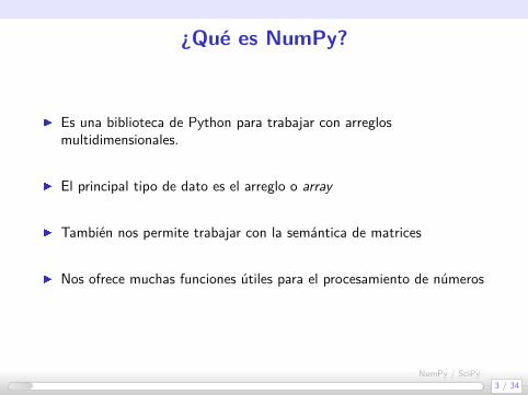
¿Qué es NumPy?

I Es una biblioteca de Python para trabajar con arreglosmultidimensionales.

I El principal tipo de dato es el arreglo o array

I También nos permite trabajar con la semántica de matrices

I Nos ofrece muchas funciones útiles para el procesamiento de números

.. . .3 / 34

.NumPy / SciPy

.

Disclaimer

I Pueden ver toda la info de esta presentación enhttp://www.scipy.org/Tentative_NumPy_Tutorial

I Los ejemplos suponen que primero se hizo en el intérprete:>>> from numpy import *

.. . .4 / 34

.NumPy / SciPy

.

El Array

I Es una tabla de elementosI normalmente númerosI todos del mismo tipoI indexados por enteros

I Ejemplo de arreglos multidimensionalesI VectoresI MatricesI ImágenesI Planillas

I ¿Multidimensionales?I Que tiene muchas dimensiones o ejesI Un poco ambiguo, mejor usar ejesI Rango: cantidad de ejes

.. . .5 / 34

.NumPy / SciPy

.

Propiedades del Array

I Como tipo de dato se llama ndarray

I ndarray.ndim: cantidad de ejes

I ndarray.shape: una tupla indicando el tamaño del array en cada eje

I ndarray.size: la cantidad de elementos en el array

I ndarray.dtype: el tipo de elemento que el array contiene

I ndarray.itemsize: el tamaño de cada elemento en el array

.. . .6 / 34

.NumPy / SciPy

.

Propiedades del Array

>>> a = arange(10).reshape(2,5)>>> aarray([[0, 1, 2, 3, 4],

[5, 6, 7, 8, 9]])>>> a.shape(2, 5)>>> a.ndim2>>> a.size10>>> a.dtypedtype('int32')>>> a.itemsize4

.. . .7 / 34

.NumPy / SciPy

.

Creando Arrays

I Tomando un iterable como origen>>> array( [2,3,4] )array([2, 3, 4])>>> array( [ (1.5,2,3), (4,5,6) ] )array([[ 1.5, 2. , 3. ],

[ 4. , 5. , 6. ]])

.. . .8 / 34

.NumPy / SciPy

.

Creando Arrays

I Con funciones específicas en función del contenido>>> arange(5)array([0, 1, 2, 3, 4])>>> zeros((2, 3))array([[ 0., 0., 0.],

[ 0., 0., 0.]])>>> ones((3, 2), dtype=int)array([[1, 1],

[1, 1],[1, 1]])

>>> empty((2, 2))array([[ 9.43647120e -268, 7.41399396e -269],

[ 1.08290285e -312, NaN]])>>> linspace(-pi, pi, 5)array([-3.141592 , -1.570796 , 0. , 1.570796 , 3.141592])

.. . .9 / 34

.NumPy / SciPy.

Manejando los ejes

>>> a = arange(6)>>> aarray([0, 1, 2, 3, 4, 5])>>> a.shape = (2, 3)>>> aarray([[0, 1, 2],

[3, 4, 5]])>>> a.shape = (3, 2)>>> aarray([[0, 1],

[2, 3],[4, 5]])

>>> a.size6

.. . .10 / 34

.NumPy / SciPy.

Operaciones básicas

I Los operadores aritméticos se aplican por elemento>>> a = arange(20, 60, 10)>>> aarray([20, 30, 40, 50])>>> a + 1array([21, 31, 41, 51])>>> a * 2array([ 40, 60, 80, 100])

I Si es inplace, no se crea otro array>>> aarray([20, 30, 40, 50])>>> a /= 2>>> aarray([10, 15, 20, 25])

.. . .11 / 34

.NumPy / SciPy.

Operaciones básicas

I Podemos realizar comparaciones>>> a = arange(5)>>> a >= 3array([False , False , False , True, True], dtype=bool)>>> a % 2 == 0array([ True, False , True, False , True], dtype=bool)

I También con otros arrays>>> b = arange(4)>>> barray([0, 1, 2, 3])>>> a - barray([20, 29, 38, 47])>>> a * barray([ 0, 30, 80, 150])

.. . .12 / 34

.NumPy / SciPy.

Operaciones básicasI Tenemos algunos métodos con cálculos típicos

>>> carray([0, 1, 2, 3, 4, 5, 6, 7, 8, 9])>>> c.min(), c.max()(0, 9)>>> c.mean()4.5>>> c.sum()45>>> c.cumsum()array([ 0, 1, 3, 6, 10, 15, 21, 28, 36, 45])

I Hay muchas funciones que nos dan info del arrayI all, alltrue, any, argmax, argmin, argsort, average, bincount, ceil, clip,

conj, conjugate, corrcoef, cov, cross, cumprod, cumsum, diff, dot, floor,inner, inv, lexsort, max, maximum, mean, median, min, minimum,nonzero, outer, prod, re, round, sometrue, sort, std, sum, trace,transpose, var, vdot, vectorize, where

.. . .13 / 34

.NumPy / SciPy.

Trabajando con los elementos

I La misma sintaxis de Python>>> a = arange(10)>>> aarray([0, 1, 2, 3, 4, 5, 6, 7, 8, 9])>>> a[2]2>>> a[2:5]array([2, 3, 4])>>>>>> a[1] = 88>>> a[-5:] = 100>>> aarray([ 0, 88, 2, 3, 4, 100, 100, 100, 100, 100])

.. . .14 / 34

.NumPy / SciPy.

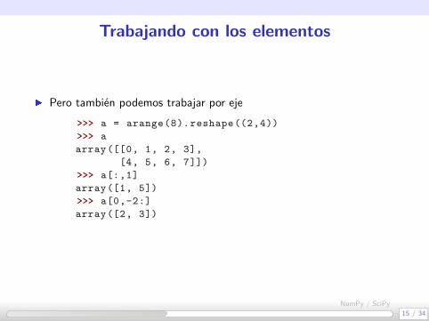
Trabajando con los elementos

I Pero también podemos trabajar por eje>>> a = arange(8).reshape((2,4))>>> aarray([[0, 1, 2, 3],

[4, 5, 6, 7]])>>> a[:,1]array([1, 5])>>> a[0,-2:]array([2, 3])

.. . .15 / 34

.NumPy / SciPy.

Cambiando la forma del arrayI Podemos usar .shape directamente

>>> a = arange(8)>>> aarray([0, 1, 2, 3, 4, 5, 6, 7])>>> a.shape = (2,4)>>> aarray([[0, 1, 2, 3],

[4, 5, 6, 7]])

I Usando .shape con comodín>>> a.shape = (4,-1)>>> aarray([[0, 1],

[2, 3],[4, 5],[6, 7]])

>>> a.shape(4, 2)

.. . .16 / 34

.NumPy / SciPy.

Cambiando la forma del array

I Transponer y aplanar>>> aarray([[0, 1, 2, 3],

[4, 5, 6, 7]])>>> a.transpose()array([[0, 4],

[1, 5],[2, 6],[3, 7]])

>>> a.ravel()array([0, 1, 2, 3, 4, 5, 6, 7])>>> aarray([[0, 1, 2, 3],

[4, 5, 6, 7]])

.. . .17 / 34

.NumPy / SciPy.

Juntando y separando arrays

I Tenemos vstack y hstack>>> a = ones((2,5)); b = arange(5)>>> aarray([[ 1., 1., 1., 1., 1.],

[ 1., 1., 1., 1., 1.]])>>> barray([0, 1, 2, 3, 4])>>> juntos = vstack((a,b))>>> juntosarray([[ 1., 1., 1., 1., 1.],

[ 1., 1., 1., 1., 1.],[ 0., 1., 2., 3., 4.]])

.. . .18 / 34

.NumPy / SciPy.

Juntando y separando arrays

I También hsplit y vsplit>>> hsplit(juntos , (1,3))[array([[ 1.],

[ 1.],[ 0.]]),

array([[ 1., 1.],[ 1., 1.],[ 1., 2.]]),

array([[ 1., 1.],[ 1., 1.],[ 3., 4.]])]

.. . .19 / 34

.NumPy / SciPy.

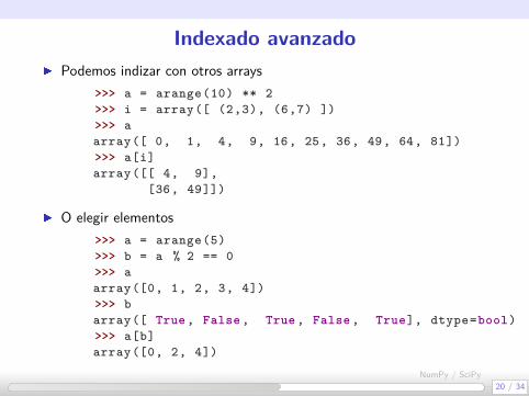
Indexado avanzadoI Podemos indizar con otros arrays

>>> a = arange(10) ** 2>>> i = array([ (2,3), (6,7) ])>>> aarray([ 0, 1, 4, 9, 16, 25, 36, 49, 64, 81])>>> a[i]array([[ 4, 9],

[36, 49]])

I O elegir elementos>>> a = arange(5)>>> b = a % 2 == 0>>> aarray([0, 1, 2, 3, 4])>>> barray([ True, False , True, False , True], dtype=bool)>>> a[b]array([0, 2, 4])

.. . .20 / 34

.NumPy / SciPy.

MatricesI Es un caso específico del array

>>> aarray([[0, 1, 2],

[3, 4, 5]])>>> A = matrix(a)>>> Amatrix([[0, 1, 2],

[3, 4, 5]])>>> A.Tmatrix([[0, 3],

[1, 4],[2, 5]])

>>> A.Imatrix([[-0.77777778 , 0.27777778],

[-0.11111111 , 0.11111111],[ 0.55555556 , -0.05555556]])

.. . .21 / 34

.NumPy / SciPy.

Matrices

I Se comportan, obviamente, como matrices>>> Amatrix([[0, 1, 2],

[3, 4, 5]])>>> Mmatrix([[2, 3],

[4, 5],[6, 7]])

>>> A * Mmatrix([[16, 19],

[52, 64]])

.. . .22 / 34

.NumPy / SciPy.

Polinomios

>>> p = poly1d([2, 3, 4])>>> print p

22 x + 3 x + 4>>> print p*p

4 3 24 x + 12 x + 25 x + 24 x + 16>>> print p.deriv()4 x + 3>>> print p.integ(k=2)

3 20.6667 x + 1.5 x + 4 x + 2>>> p(range(5))array([ 4, 9, 18, 31, 48])

.. . .23 / 34

.NumPy / SciPy.

SciPy

.. . .24 / 34

.NumPy / SciPy.

Intro

I Colección de algoritmos matemáticos y funciones

I Construido sobre NumPy

I Poder al intérprete interactivo

I Procesamiento de datos y prototipado de sistemasI Compite con Matlab, IDL, Octave, R-Lab, y SciLab

.. . .25 / 34

.NumPy / SciPy.

Disclaimer

I Pueden ver toda la info de esta presentación enhttp://docs.scipy.org/doc/

I ¿Les conté que me recibí de ingeniero hace más de 9 años?

.. . .26 / 34

.NumPy / SciPy.

Funciones y funciones!

I De todo tipo!I airyI ellipticI besselI gammaI betaI hypergeometricI parabolic cylinderI mathieuI spheroidal waveI struveI kelvin

.. . .27 / 34

.NumPy / SciPy.

Integration

I General integration

I Gaussian quadrature

I Integrating using samples

I Ordinary differential equations

.. . .28 / 34

.NumPy / SciPy.

Optimization

I Nelder-Mead Simplex algorithmI Broyden-Fletcher-Goldfarb-Shanno algorithmI Newton-Conjugate-GradientI Least-square fittingI Scalar function minimizersI Root finding

>>> f = poly1d([1, 4, 8])>>> print f

21 x + 4 x + 8>>> roots(f)array([-2.+2.j, -2.-2.j])>>> f(-2.+2.j)0j

.. . .29 / 34

.NumPy / SciPy.

Interpolation

I Linear 1-d interpolationI Spline interpolation in 1-dI Two-dimensional spline representation

.. . .30 / 34

.NumPy / SciPy.

Signal Processing

I B-splinesI second- and third-order cubic spline coefficientsI from equally spaced samples in one- and two-dimensions

I FilteringI Convolution/CorrelationI Difference-equation filteringI Other filters: Median, Order, Wiener, Hilbert, ...

.. . .31 / 34

.NumPy / SciPy.

Algebra lineal

I MatricesI InversasI DeterminantesI Resolución de sistemas lineales

I DescomposicionesI Eigenvalues and eigenvectorsI Singular value, LU, Cholesky, QR, Schur

I Funciones de matricesI Exponentes y logaritmosI Trigonometría (común e hiperbólica)

.. . .32 / 34

.NumPy / SciPy.

Estadísticas

I Masked statistics functionsI 64!

I Continuous distributionsI 81!

I Discrete distributionsI 12!

I Statistical functionsI 72!

.. . .33 / 34

.NumPy / SciPy.

¡Muchas gracias!¿Preguntas?

¿Sugerencias?

Facundo Batistafacundo@taniquetil.com.ar

http://www.taniquetil.com.ar

Licencia: Creative CommonsAtribución-NoComercial-CompartirDerivadasIgual 2.5 Argentinahttp://creativecommons.org/licenses/by-nc-sa/2.5/deed.es_AR

.. . .34 / 34

.NumPy / SciPy.