NUMERICAL STUDY OF AEROELASTIC BEHAVIOUR OF A TROPOSKIEN SHAPE VERTICAL AXIS WIND TURBINE ·...

NUMERICAL STUDY OF AEROELASTICBEHAVIOUR OF A TROPOSKIEN SHAPE VERTICAL

AXIS WIND TURBINE

A thesis submitted tothe Faculty of Graduate and Postdoctoral Affairs

in partial fulfillment of the requirements for the degree

Masters of Applied Science

by

Amin Fereidooni

The Department of Mechanical and Aerospace EngineeringCarleton University

September 2013

©2013 Amin Fereidooni

Abstract

A methodology for aeroelastic analysis of Vertical Axis Wind Turbines (VAWTs) with

troposkien geometry is developed. The structural dynamic equations used in this analysis

represent the behaviour of a three dimensionally curved beam in terms of generalized force

and generalized displacement vectors. This linear formulation takes into account the effect

of the Coriolis forces and centrifugal stiffening. It is demonstrated that the mixed form of

the equations lends itself well to the application of mixed finite element method.

The structural dynamic equations are coupled with a free vortex based aerodynamic

model. The aerodynamic model represents the wake with a cluster of vortex filaments that

stretch, rotate and translate freely in the wake of the wind turbine. The unsteady effect of

the wake is already taken into consideration when the aerodynamic forces on the blades

are evaluated by interpolating the force coefficients from input experimental airfoil data. It

is illustrated that in the case of strong vortex-blade interaction at high tip speed ratio, this

model can tackle the problem with high accuracy.

The computational aeroelastic framework is utilized to study the aeroelastic behaviour

of the 17-meter DOE-Sandia VAWT. It is shown that in the operating range of the wind

turbine, the structural vibration has minimum effect on the aerodynamic performance of

the turbine. Furthermore, the comparison of the estimated vibratory stress at the root of

wind turbine with the experimental data reveals excellent agreement except at the region

where dynamic stall plays a crucial role in predicting the aerodynamic forces.

ii

Acknowledgments

I would like to extend my gratitude to my supervisors Professor Fred Nitzsche and Pro-

fessor Edgar Matida for providing an open, friendly and collaborative research environ-

ment. I would like to thank Professor Nitzsche for teaching me how to think as an inde-

pendent researcher. I appreciate Professor Matida for his help any time I had to deal with a

challenging situation.

I would also like to thank my friends and former colleagues Anton Matachniouk, Dr.

Waad Subber, Dr. Mohammad Khalil, Adam Walker and Hamza Ella for assisting me in

my learning process and for making this period of life an enjoyable one. I wish to thank

my current colleagues Hali Barber, Basim Altalua, Doma Suliman and Souhib Aljasim for

their help and support.

Furthermore, I thank my family. I am indebted to my parents whose love, support and

understanding helped me to pursue graduate studies. Last but not least, I would like to

thank my girlfriend, Mahkameh Yaghmaie, for providing me support, encouragement and

motivation throughout the course of my studies.

iii

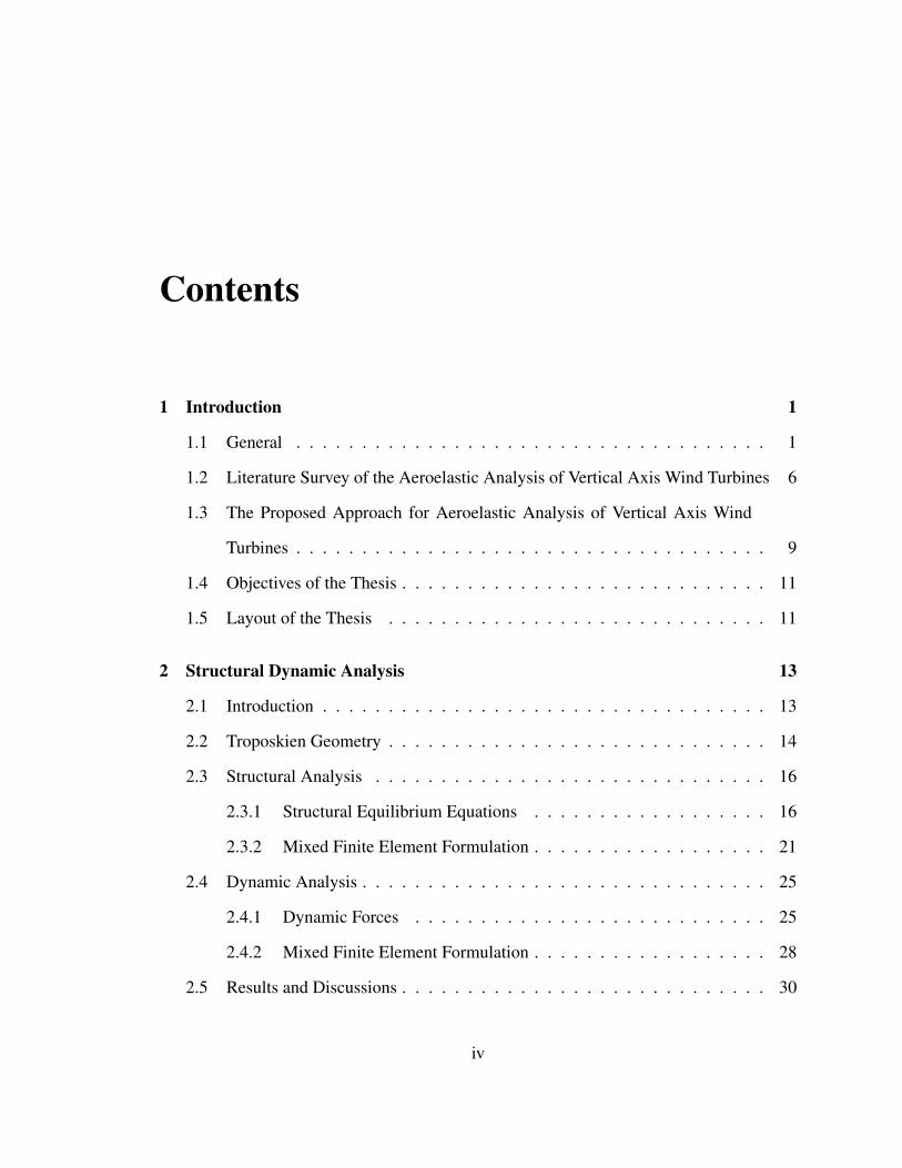
Contents

1 Introduction 1

1.1 General . . . . . . . . . . . . . . . . . . . . . . . . . . . . . . . . . . . . 1

1.2 Literature Survey of the Aeroelastic Analysis of Vertical Axis Wind Turbines 6

1.3 The Proposed Approach for Aeroelastic Analysis of Vertical Axis Wind

Turbines . . . . . . . . . . . . . . . . . . . . . . . . . . . . . . . . . . . . 9

1.4 Objectives of the Thesis . . . . . . . . . . . . . . . . . . . . . . . . . . . . 11

1.5 Layout of the Thesis . . . . . . . . . . . . . . . . . . . . . . . . . . . . . 11

2 Structural Dynamic Analysis 13

2.1 Introduction . . . . . . . . . . . . . . . . . . . . . . . . . . . . . . . . . . 13

2.2 Troposkien Geometry . . . . . . . . . . . . . . . . . . . . . . . . . . . . . 14

2.3 Structural Analysis . . . . . . . . . . . . . . . . . . . . . . . . . . . . . . 16

2.3.1 Structural Equilibrium Equations . . . . . . . . . . . . . . . . . . 16

2.3.2 Mixed Finite Element Formulation . . . . . . . . . . . . . . . . . . 21

2.4 Dynamic Analysis . . . . . . . . . . . . . . . . . . . . . . . . . . . . . . . 25

2.4.1 Dynamic Forces . . . . . . . . . . . . . . . . . . . . . . . . . . . 25

2.4.2 Mixed Finite Element Formulation . . . . . . . . . . . . . . . . . . 28

2.5 Results and Discussions . . . . . . . . . . . . . . . . . . . . . . . . . . . . 30

iv

2.5.1 Coriolis Force Excluded . . . . . . . . . . . . . . . . . . . . . . . 31

2.5.2 Coriolis Force Included . . . . . . . . . . . . . . . . . . . . . . . . 36

2.6 Conclusions . . . . . . . . . . . . . . . . . . . . . . . . . . . . . . . . . . 40

3 Aerodynamic Analysis 41

3.1 Introduction . . . . . . . . . . . . . . . . . . . . . . . . . . . . . . . . . . 41

3.2 Free Vortex Model . . . . . . . . . . . . . . . . . . . . . . . . . . . . . . 42

3.2.1 Coordinate System . . . . . . . . . . . . . . . . . . . . . . . . . . 42

3.2.2 Element Bound Vorticity . . . . . . . . . . . . . . . . . . . . . . . 43

3.2.3 Vortex Shedding . . . . . . . . . . . . . . . . . . . . . . . . . . . 45

3.2.4 Wake Convection . . . . . . . . . . . . . . . . . . . . . . . . . . . 47

3.2.5 Remarks . . . . . . . . . . . . . . . . . . . . . . . . . . . . . . . 48

3.3 Numerical Validation . . . . . . . . . . . . . . . . . . . . . . . . . . . . . 50

3.4 Convergence Analysis . . . . . . . . . . . . . . . . . . . . . . . . . . . . 55

3.4.1 Spatial Convergence . . . . . . . . . . . . . . . . . . . . . . . . . 55

3.4.2 Temporal Convergence . . . . . . . . . . . . . . . . . . . . . . . . 55

3.5 Parallel Implementation . . . . . . . . . . . . . . . . . . . . . . . . . . . . 57

3.6 Conclusions . . . . . . . . . . . . . . . . . . . . . . . . . . . . . . . . . . 59

4 Aeroelastic Analysis 61

4.1 Introduction . . . . . . . . . . . . . . . . . . . . . . . . . . . . . . . . . . 61

4.2 Aeroelastic Coupling . . . . . . . . . . . . . . . . . . . . . . . . . . . . . 62

4.2.1 Structural Deflection . . . . . . . . . . . . . . . . . . . . . . . . . 62

4.2.2 Aerodynamic Updates . . . . . . . . . . . . . . . . . . . . . . . . 65

4.3 Results and Discussions . . . . . . . . . . . . . . . . . . . . . . . . . . . . 69

4.3.1 Aerodynamic Performance . . . . . . . . . . . . . . . . . . . . . . 70

v

4.3.2 Structural Performance . . . . . . . . . . . . . . . . . . . . . . . . 73

4.4 Conclusions . . . . . . . . . . . . . . . . . . . . . . . . . . . . . . . . . . 81

5 Conclusions and Recommendations 82

5.1 Summary . . . . . . . . . . . . . . . . . . . . . . . . . . . . . . . . . . . 82

5.2 Conclusion . . . . . . . . . . . . . . . . . . . . . . . . . . . . . . . . . . 83

5.3 Recommendations and Future Work . . . . . . . . . . . . . . . . . . . . . 84

Appendices 86

A Appendix A: Aerodynamic Updates due to the Structural Vibration 86

A.1 Coordinate Systems and Transformation Matrices . . . . . . . . . . . . . . 86

A.2 Absolute Displacement of the Aerodynamic Centre due to the Structural

Displacement . . . . . . . . . . . . . . . . . . . . . . . . . . . . . . . . . 88

A.3 Rotation of the Blade Section due to the Structural Displacement . . . . . 90

A.4 Absolute Velocity of the Aerodynamic Centre due to the Structural Velocity 91

References 94

vi

List of Tables

2.1 Phase information of the first and second mode shapes . . . . . . . . . . . 37

vii

List of Figures

1.1 (a) A typical troposkien shape Vertical Axis Wind Turbine (VAWT) adapted

from reference [1] (b) A typical Horizontal Axis Wind Turbine (HAWT)

adapted from reference [2] . . . . . . . . . . . . . . . . . . . . . . . . . . 2

1.2 Life cycle cost breakdown of a typical baseline offshore wind project [2] . . 4

2.1 DOE-Sandia 17-meter Darrieus vertical axis wind turbine (a) Geometry

specifications (dimensions in meter) (b) Coordinate system . . . . . . . . . 17

2.2 Blade cross section of the DOE-Sandia 17-meter vertical axis wind turbine:

extruded aluminium, NACA0015 . . . . . . . . . . . . . . . . . . . . . . . 17

2.3 (a) Components of the generalized displacement yD (b) Components of the

generalized force yF . . . . . . . . . . . . . . . . . . . . . . . . . . . . . 19

2.4 Blade cross section: definitions . . . . . . . . . . . . . . . . . . . . . . . . 20

2.5 Variation of the first and second natural frequencies (ω1, ω2) with the an-

gular velocity of the vertical axis wind turbine Ω: no centre of mass offset

( xα = 0.0), Coriolis effect excluded. (a) KDD included (b) KDD excluded . 32

2.6 First two mode shapes: angular velocity Ω = 50.6 rpm, no centre of mass

offset ( xα = 0), Coriolis effect excluded. (a) Plunge displacement (b)

Chordwise displacement (c) Spanwise displacement (d) Pitch displacement 34

viii

2.7 First two mode shapes: angular velocity Ω = 50.6 rpm, 10% centre of mass

aft ( xα = −0.1), Coriolis effect excluded. (a) Plunge displacement (b)


2.8 First two mode shapes: angular velocity Ω = 50.6 rpm, no centre of mass

offset ( xα = 0), Coriolis effect included. (a) Plunge displacement (b)


2.9 The fan plot of the DOE-Sandia 17-meter Darrieus vertical axis wind tur-

bine: operating angular velocity Ω = 50.6 rpm, 10% centre of mass aft (

xα = −0.1), Coriolis effect included. . . . . . . . . . . . . . . . . . . . . . 39

3.1 Free vortex model conventions (a) Blade element local coordinate system

(b) Global coordinate system . . . . . . . . . . . . . . . . . . . . . . . . . 44

3.2 Vortex shedding for a single blade element . . . . . . . . . . . . . . . . . . 47

3.3 Induced velocity at a point by vortex filament . . . . . . . . . . . . . . . . 49

3.4 Comparison of equator forces between the FEM-Vort aerodynamic and

VDART3: chord to equator ratio of CR

= 0.135, height to radius ratio of

HR= 2, tip speed ratio of RΩ

U∞= 5, FEM-Vort with fixed Reynolds number . 51

3.5 Comparison of equator forces between the FEM-Vort aerodynamic and

VDART3: chord to equator ratio of CR

= 0.135, height to radius ratio of

HR= 2, tip speed ratio of RΩ

U∞= 5, FEM-Vort with variable Reynolds number 53

3.6 The FEM-Vort aerodynamic model: height H = 2m, equator radius R =

1m, chord length C = 0.135m, the wind turbine angular velocity Ω =

45 rad/s and the wind velocity U∞ = 9m/s (a) Variation of angle of

attack (b) Variation of Reynolds number (c) Variation of lift coefficient at

AOA = 10 with Reynolds number . . . . . . . . . . . . . . . . . . . . . 54

ix

3.7 Convergence analysis: 17 meter DOE-Sandia VAWT, the wind turbine an-

gular velocity Ω = 50.6 rpm and the wind velocity U∞ = 22mph (a)

Number of blade elements (b) Number of time steps per revolution . . . . . 56

3.8 Verification of the parallel implementation in terms of the tangential force

coefficient: comparison of the serial and the parallel (using 24 CPUs) im-

plementations, 17 meter DOE-Sandia VAWT, 23 blade elements, 10 revo-

lutions, 40 steps per revolution . . . . . . . . . . . . . . . . . . . . . . . . 59

3.9 Scalability of parallel implementation: 17 meter DOE-Sandia VAWT, 23

blade elements, 10 revolutions, 40 steps per revolution (a) Computer run

time (b) Speedup . . . . . . . . . . . . . . . . . . . . . . . . . . . . . . . 59

4.1 (a) Aerodynamic forces on the blade section (b) Rotating frame of reference 63

4.2 Comparison of the generated torque: 17-meter DOE-Sandia VAWT, oper-

ating angular velocity Ω = 50.6 rpm (a) Tip speed ratio = 2.18 (b) Tip

speed ratio = 2.8 (c) Tip speed ratio = 4.36 . . . . . . . . . . . . . . . . . . 71

4.3 The power curve of the DOE-Sandia 17 meter VAWT: operating angular

velocity Ω = 50.6 rpm . . . . . . . . . . . . . . . . . . . . . . . . . . . . 72

4.4 Wake structure: 17-meter DOE-Sandia VAWT, operating angular velocity

Ω = 50.6 rpm, tip speed ratio = 4.36, azimuth angle (θ) = 1890 . . . . . . 73

4.5 Elastic axis displacement at the equator of the 17-meter DOE-Sandia VAWT:

operating angular velocity Ω = 50.6 rpm, tip speed ratio = 4.36 (a) Trans-

lational displacement (b) Rotational displacement . . . . . . . . . . . . . . 75

4.6 Frequency content of the elastic axis displacement at the equator of the 17-

meter DOE-Sandia VAWT: operating angular velocity Ω = 50.6 rpm, tip

speed ratio = 4.36 (a) Translational displacement (b) Pitch displacement . . 75

x

4.7 Elastic axis internal forces at the root of the 17-meter DOE-Sandia VAWT:

operating angular velocity Ω = 50.6 rpm, tip speed ratio = 4.36 (a) Mo-

ment about plunge axis (b) Moment about chordwise axis (c) Axial force . . 77

4.8 Axial strain at the root of the 17-meter DOE-Sandia VAWT: operating an-

gular velocity Ω = 50.6 rpm, tip speed ratio = 4.36 (a) Elastic axis (b)

Trailing edge . . . . . . . . . . . . . . . . . . . . . . . . . . . . . . . . . 78

4.9 Axial stress at the root of the 17-meter DOE-Sandia VAWT: operating an-

gular velocity Ω = 50.6 rpm, tip speed ratio = 4.36 (a) Elastic axis (b)

Trailing edge . . . . . . . . . . . . . . . . . . . . . . . . . . . . . . . . . 79

4.10 Elastic axis axial stress along the blades of the 17-meter DOE-Sandia VAWT:

operating angular velocity Ω = 50.6 rpm, tip speed ratio = 4.36, azimuth

angle (θ) = 1890 . . . . . . . . . . . . . . . . . . . . . . . . . . . . . . 80

4.11 Trailing edge vibratory stress at the root of the DOE-Sandia 17-meter VAWT:

operating angular velocity Ω = 50.6 rpm . . . . . . . . . . . . . . . . . . 81

A.1 (a) Coordinate systems (b) Blade section displacement . . . . . . . . . . . 93

xi

Nomenclature

Latin Symbols

A (scalar) area of the blade cross section

A (matrix) state-space matrix

AF wind turbine swept area

a0 dimensionless structural parameter

BN blade number

b blade semichord

C chord length

CD, CL, CM aerodynamic drag, lift and moment coefficients

CN , CT aerodynamic normal and tangential force coefficients

CP power coefficient

CQ torque coefficient

c the elliptic integral parameter

d0 distance between the elastic axis and the aerodynamic centre of the blade

cross section

E Young’ modulus

E (ϕ; c) elliptic integral of the second kind

EA axial stiffness

EIij bending stiffness, (ij = xx, yy, xy)

xii

e1, e2, e3 unit triad defining the undisturbed position of the elastic axis

e′1, e′2, e′3 unit triad defining the perturbed position of the elastic axis

er, eθ, eζ unit triad defining the rotating frame of reference

F external force vector in finite element method

FN , FT total normal and tangential forces generated by the aerodynamic blade el-

ement

F (ϕ; c) elliptic integral of the first kind

f , fA, fD generalized total, aerodynamic and dynamic external force vector

f1D, f2

D, f 2D components of the dynamic force vector

f1, f2, f3 components of the external force acting on the blade cross section

fss generalized steady state dynamic force vector

f iss components of the generalized steady state dynamic force vector,

(i = 1, 2, ..., 6)

G shear modulus

GA shear stiffness

GIα torsional stiffness

H total height of the blade

h half of the total height of the blade

i, j, k unit triad defining the inertial reference frame

KD dynamic stiffness matrix

KDD displacement block matrix constructing the structural stiffness matrix

KDF displacement-force coupling block matrix constructing the structural stiff-

ness matrix

KFD force-displacement coupling block matrix constructing the structural stiff-

ness matrix

xiii

KFF force block matrix constructing the structural stiffness matrix

l total length of the blade along s coordinate

le aerodynamic blade element length

M , C, K mass matrix, Coriolis matrix, stiffness matrix

M1, M2, M3 components of the internal bending moment of the blade cross section

m1, m2, m3 components of the external moment acting on the blade cross section

m1D, m2

D, m3D components of the dynamic moment vector

ND, NF displacement and force vector shape functions

NB number of blades

NE number of aerodynamic blade elements for each blade

NTI number of time increments

Q1, Q2, τ internal force of the blade cross section

R wind turbine equator radius

Re Reynolds number

r radius of the blade section from the vertical axis of the wind turbine

rα radius of gyration of the cross section

s, c, n unit triad defining the aerodynamic blade element

T , N , M tangential force, normal force and moment distributed over the aerody-

namic blade element

U , V , W components of the vortex induced velocity

UR total velocity assigned to each aerodynamic blade element

Ut blade velocity

U∞ wind velocity

u, v, w local translational displacement of the elastic axis

X , Y , Z global coordinates of the aerodynamic centre

xiv

xα dimensionless distance between the elastic axis and the centre of mass of

the blade cross section in semichord

x(n) dimensionless distance between the elastic axis and the neutral centre of

the blade cross section in semichord

Y state-space vector

yD, yF generalized displacement and force vectors

ZDD coefficient matrix containing displacement dependent structural terms

ZDF coefficient matrix containing displacement-force coupling structural terms

ZFD coefficient matrix containing force-displacement coupling structural terms

ZFF coefficient matrix containing force dependent structural terms

Greek Symbols

α angle of attack

β ratio of the equator radius to half of the height of the wind turbine

ΓB, ΓS , ΓT bound vortex, spanwise vortex, trailing tip vortex strength

∆t time increment

∆X , ∆Y , ∆Z components of the aerodynamic centre movement due to the structural vi-

bration

∆c rotation of the chordwise axis due to the structural vibration

∆x, ∆y, ∆z components of the vortex displacement

εac, εea perturbation of the aerodynamic centre and elastic axis

εss, σss axial strain and stress

ζ vertical coordinate of the troposkien

θ azimuth angle

θB blade azimuth angle

xv

xvi

κ(0) initial local curvature of the troposkien shape

λ ratio of the second moment of area about e1 to the polar moment of area

ν air kinematic viscosity

ρ air density

σ density of the material of the blade

τ (0), τ (0)min initial local tension of the blade and its minimum

ϕ troposkien parameter

φ local angle of the troposkien

χ1, χ2, α local rotational displacement of the elastic axis

Ω, Ω vector of the angular velocity of the turbine and its magnitude

ω natural frequency of the system

Chapter 1

Introduction

1.1 General

The world is currently facing an energy dilemma, the fossil fuel is diminishing in supply

while the demand for energy is increasing. This has motivated many countries to invest

in harnessing energy from renewable resources. Among these resources, wind power is

one of the fastest growing sectors. The most efficient approach for extracting the kinetic

energy of the wind is the use of lift-driven wind turbines. These wind turbines are generally

categorized into two groups: Horizontal Axis Wind Turbine (HAWT) and Vertical Axis

Wind Turbine (VAWT). Fig.1.1 shows a typical VAWT and HAWT. Although both wind

turbines offer the same ideal efficiency [3], HAWTs hold a number of advantages over

VAWTs: firstly, the HAWTs are self-starting machines, which eliminates the need for an

auxiliary starter [4]. Secondly, for the same swept area, the VAWTs’ blade length is two to

three times greater that the HAWTs counterpart [4], and thirdly the HAWTs’ aerodynamic

performance is much simpler than the VAWTs [3]. The distribution of aerodynamic loading

along the blades of a VAWT changes with respect to the azimuth angle; hence, leading

1

2

to cyclic stress fatigue of the components [5]. Another complexity of the aerodynamic

behaviour of VAWTs stems from the fact that the blades might encounter their wake as

well as the vortices generated by other blades during one revolution. As a result, land-

based HAWTs are the most commonly used wind turbines around the world.

(a) (b)

Figure 1.1: (a) A typical troposkien shape Vertical Axis WindTurbine (VAWT) adapted from reference [1] (b) A typical

Horizontal Axis Wind Turbine (HAWT) adapted from reference [2]

As the demand for reducing the reliance on the fossil fuels increases around the world,

nations are striving to find better ways to increase clean energy capacities. In the field of

wind power, this has prompted the initiatives of moving wind turbines towards offshore

application. For instance, in 2010, the National Renewable Energy Laboratory (NREL) of

the United States estimates that U.S. offshore wind has a gross potential generating capacity

four times greater than the nation’s present electric capacity [2]. In general, the offshore

wind power offers the following benefits [2]:

• Wind speed increases with the distance from the coast significantly. This increase in

3

the wind speed could lead to a 29% increase in the annual average energy production

as reported by NREL.

• Less restrictive offshore transportation equipments allow installation of larger wind

turbines.

• Land-based wind farms, which are typically far from the inhabited areas, require a

considerable transmission capacity. Offshore wind power, which is relatively close

to the coastal load centres mitigates this need; thus, it makes the energy production

more cost-effective.

• With the development of the technology which facilitates the installation of wind

turbines in deep water, the visible impact of wind turbine would become minimum.

• The deep water offshore installation sites also reduce the possibility of sound propa-

gation problems in the coastal areas.

One of the major obstacles in using the offshore wind power is the higher costs associated

with this technology compared to the land-based wind turbines. The existing uncertainties

in the hydrodynamic loadings of offshore platforms urge the adoption of more conservative

structural designs, leading to more costs. In addition, Operation and Maintenance (O &

M) costs in an offshore wind turbine is almost two to three times greater than a land-based

wind turbine [2]. NREL [2] gives an estimate of the life-cycle cost breakdown of a typical

baseline offshore wind project, shown in Fig.1.2.

Currently, efforts are being made to reduce the total costs of offshore wind power to

rationalize the use of this technology when compared to the land-based wind turbines. This

effort initiated a reviving interest in VAWT offshore applications. For instance, the U.S.

department of energy has put forward a five year project regarding innovative offshore

4

Figure 1.2: Life cycle cost breakdown of a typical baseline offshore windproject [2]

vertical axis wind turbine rotors pursued by Sandia National Laboratory and a number

of U.S. universities [1]. This interest hinges on the advantages of VAWTs as a potential

alternative to offshore HAWTs:

• VAWTs are responsive to the wind regardless of its direction. Conversely, HAWTs

need to have a yawing system that adds complexity to the drive train.

• VAWTs operate at both stalled and unstalled conditions. However the stall properties

of the blade removes the need for control pitch mechanism.

• Gearbox and generator of the VAWTs are placed at the bottom of the wind turbine;

therefore, they are more accessible compared to HAWTs’. This valuable charac-

teristic could reduce the cost for Operation and Maintenance (O & M) in offshore

applications substantially.

• Since the heavy components of the VAWTs, generator and gearbox, are placed at the

bottom of the wind turbine, the centre of gravity of the entire system is closer to the

sea level. This fact helps the system to be more stable by nature, resulting in less

costly support structures.

5

• As mentioned earlier, one of the advantages of the offshore wind power is the possi-

bility of building larger rotors. For HAWTs, this advantage conflicts with the fact that

the larger wind turbine becomes heavier and the cyclic effect of the weight causes

fatigue problems. On the contrary, weight of the blade does not generally become

restrictive in the design of VAWTs.

According to the aforementioned discussions, it seems that VAWTs have the potential to

outperform HAWTs especially for the offshore applications. Therefore, further research

seems to be necessary to fully understand the behaviour of this type of wind turbine for

offshore applications. One of the major challenges in this type of applications is with

regards to the hydrodynamic loading at the base of the wind turbine. The wave induced

movement of the base of the wind turbine not only affects the performance of the wind

turbine but also demands specially designed support structures. The design of support

structures becomes a significantly crucial step when deep-water installation is concerned.

However, in light of future research efforts, better designs of this type of wind turbine

could alleviate these challenges in such a way that their future use become more feasible.

Perhaps, one of the very first steps aims at a deeper understanding of the land-based version

of the VAWTs.

The focus of the current thesis is the study of the aeroelastic behaviour of a land-based

VAWT. The type of VAWT chosen for this investigation is a Darrieus type with troposkien

shape blades. Troposkien blades are referred to as the ones having the shapes that look

like a rope spinning about a vertical axis while it is fixed at its ends. More details of the

methodology implemented in this thesis is described in the following sections.

6

1.2 Literature Survey of the Aeroelastic Analysis of Verti-

cal Axis Wind Turbines

In general, there are two categories of aerodynamic models of VAWTs: momentum theory

and vortex theory based models. The first momentum based model was proposed by Tem-

plin in 1974 [6]. In this model, it is assumed that a streamtube passes through the rotor, and

inside this streamtube the induced velocity is constant everywhere. Then, the drag forces

are calculated based on this constant induced velocity at the blades. Equating the drag

force to the change of momentum caused by the rotor allows the calculation of the induced

velocity. In order to enhance the assumption of constant induced velocity everywhere on

the blade, Strickland [7] developed the multiple streamtube model, by assuming multiple

streamtubes which pass through the swept volume of the rotor. Based on this assumption,

the induced velocity can change at different locations along the blade. Although the multi-

ple streamtube model is more successful in predicting the performance of the wind turbine,

it still suffers from the fact that, inside one streamtube, it does not distinguish between

the upwind and downwind position of the rotor. To relax this assumption, Paraschivoiu

[8] developed the double multiple streamtube model, where two separate sets of multiple

streamtubes represent the aerodynamics of the upwind and downwind of the wind turbine.

Although momentum based models are very efficient methods in terms of execution time,

they inherit the deficiencies that are present in momentum theory. The root of these defi-

ciencies originates from the fact that these models do not explicitly take into account the

effect of vortices. In VAWTs, as the tip speed ratio increases, it is more likely that each

blade catches with its own vortices and the ones generated by other blades. The same

phenomenon occurs when more blades are added to the wind turbine, in other words, the

solidity increases. In these cases, the capability of momentum based models in predicting

7

not only the loads on the blade but also the performance degrades. Moreover, these models

cannot provide any information about the near wake structure of the flow. This information

is significantly important when the interaction of the wake with downstream wind turbine

in a wind farm setting is of interest.

The second category of the VAWTs’ aerodynamic models are vortex theory based mod-

els that are more computationally expensive but more accurate in estimating the aerody-

namic loads in a VAWT. Strickland et al. [9] developed a three dimensional free vortex

model for the study of Darrieus type VAWTs. One of the advantages of this model is that,

unlike momentum based models, it fully takes into account the unsteady effects of the vor-

tices by representing these vortices as filaments which convect freely in the fluid domain.

This characteristic allows the calculation of the induced velocity everywhere in the domain,

including the velocity at the blades. Therefore, this model is capable of predicting the aero-

dynamic loads more accurately. The strength of this method becomes even more evident

when the blade-vortex interaction becomes stronger, e.g., at high tip speed ratios or high

solidity ratios. As the second advantage, this model provides useful information about the

near wake structure of flow downstream of the wind turbine.

Although the execution time of the free vortex method mentioned above is a lot less than

a full CFD simulation, there were concerns, at the time of its development in the 1980s,

regarding the restrictions that this method imposes in engineering analysis specifically due

to the computer simulation run time. In an effort to tackle this challenge, Wilson and Walker

[10] combined the streamtube model with the vortex method to reduce the computer run

time. Strickland [11] also suggested few techniques for similar purpose at the expense

of loosing the spectral accuracy to certain degrees. However, it is worth mentioning that

with the current computational power available in typical laptops alongside with parallel

processing capabilities such as MPI and OpenMP, the time required for these types of

8

analyzes could be reduced significantly.

Besides the aerodynamic efficiency of the VAWTs, another aspect that plays an impor-

tant role in justifying wind power technology as a renewable resource is relatively low

cost associated with the fatigue life of the components such as the blades. Veers [5] high-

lights the importance of estimating the time history of stress for the fatigue analysis of the

VAWTs. The need for an acceptable estimation of stress in VAWTs underlines the necessity

of structural dynamic and aeroelastic analysis as a crucial part of VAWTs’ study. Numer-

ous researchers have addressed different aspects of the aeroelastic analysis of VAWTs, in

particular, one could refer to the reports from the Sandia National Laboratory in the 1980s.

Lobitz [12] developed the transient dynamic analysis package (VAWTDYN) for the

analysis of VAWTs, which utilizes the single streamtube aerodynamic model. VAWDYN

is used to predict the vibratory stress at the root of DOE-Sandia 17-meter VAWT. The com-

parison of the results with the available experimental data reveals limited success mainly

due to the inaccurate prediction of the loads by the single streamtube model. Watson [13]

compares the predictions of a non-linear finite element analysis with the strain gauge mea-

surements on the DOE-Sandia 17-meter VAWT. In this analysis, the effect of only cen-

trifugal and gravitational forces are considered. Carne et al. [14] derived the structural

dynamic equations for a rotating structure while ignoring the aerodynamic forces. They

perform a modal analysis to compare the predicted mode shapes and frequencies with the

experimental data available for the Sandia 2-meter vertical axis wind turbine. In their anal-

ysis, which is developed in the finite element framework, rotational degrees of freedom and

their corresponding kinetic energy are neglected. Lobitz and Sullivan [15] apply a similar

finite element derivation to evaluate the forced response of the DOE-Sandia low cost 17-

meter blade to the aerodynamic loading. Two aerodynamic models are utilized: the single

streamtube model and the double multiple streamtube model. It is shown that although the

9

agreement of the numerical results with the experimental data is encouraging, it does not

absolutely predict all response details with high accuracy [15]. One of the sources of error

mentioned in this report is the uncertainty in aerodynamic load prediction.

Nitzsche [16] distinctively derived a rigorous set of dynamic equations of motion that

accounts for the Coriolis effect, centrifugal softening and centrifugal stiffening. These

equations are coupled with the quasi-steady aerodynamic loading in order to assess the

aeroelastic instability of the VAWTs. The aerodynamic loading which is based on the

Theodorsen’s theory does not take into account the stall conditions, wake effect and the

unsteadiness of the flow. Popelka [17] also formulates a similar set of structural dynamic

equations for the troposkien shape blades. In these equations, the effects of tower and the

drive train are also modelled by torsional springs. In Popelka’s analysis, a Theodorsen

based aerodynamic model is adopted for the unsteady effects; however, the wake effect and

the stall conditions are neglected.

1.3 The Proposed Approach for Aeroelastic Analysis of

Vertical Axis Wind Turbines

As emphasized in the previous section, all of the aeroelastic analyzes performed on the

VAWTs so far suffer from the lack of a robust aerodynamic modelling. They use a momen-

tum based model combined with either the experimental data or the Theodorsen’s theory.

Both of these models do not take into consideration the wake effect rigorously. In an at-

tempt to alleviate such problem, the free vortex model proposed by Strickland et al. [9] is

adopted in the current investigation. Furthermore, two new features are integrated with the

original model proposed by Strickland et al. [9]:

• The original model by Strickland only uses the set of experimental data that corre-

10

sponds to the equator maximum Reynolds number. This assumption is not truly valid

because not only the magnitude of the blade velocity changes at different sections

along the blade but also its angle with the wind velocity changes with the azimuth

angle of the turbine. Therefore, the Reynolds number associated with the relative

velocity changes along the blade as well as in time. In the current study, the effect of

variable Reynolds number is taken into account by using interpolation between the

experimental data available for a wide range of Reynolds number.

• In order to reduce the computer run time of the model, the method is parallelized by

taking advantage of the shared-memory parallel programming interface, OpenMP.

The structural dynamic equations implemented in this study are the ones devised by Nitzsche

[16]. Nitzsche represents the structural dynamic behaviour of a three dimensional linear

curved beam with troposkien shape in a state vector form. This state vector consists of

12-first order linear ordinary differential equations, based on generalized force and gen-

eralized displacement variables. This formulation explicitly represents the effect of the

Coriolis forces, centrifugal softening and tensile stress caused by the centrifugal forces.

Nitzsche applies a frequency domain based method, namely Transfer Matrix method, to

examine the stability of the system. Here, due to the mixed nature of the equations, as op-

posed to the irreducible form, the equations are cast into a mixed finite element formulation

and the response of the system is calculated in time.

Finally, the structural dynamic equations, in mixed finite element form, are coupled with

the free vortex model. The aeroelastic analysis tool, named FEM-Vort, is used to predict

aerodynamic performance and structural responses of the DOE-Sandia 17-meter VAWT.

The numerical results are compared with the available experimental data.

11

1.4 Objectives of the Thesis

The objectives of the thesis are as follows:

• Aerodynamic analysis: the aerodynamic model is a combination of the free vortex

model with the lift and drag coefficients obtained from the experimental data. One

of the primary objectives of this study is to investigate the accuracy of this model in

estimating the aerodynamic loading on the blade. Secondly, it is of interest of this

study to assess the structure of the wake and its influence on the performance of the

wind turbine.

• Structural dynamic analysis: the main objective of the structural dynamic analysis

is to evaluate the effect of the Coriolis and centrifugal forces on the characteristic of

the system.

• Aeroelastic analysis: The ultimate goal of this investigation is to predict the time

history of the strain and stress along the blade at different tip speed ratio and locate

the high stress part of the blade.

1.5 Layout of the Thesis

Chapter (2): it begins with the structural dynamic equations used in this thesis. The appli-

cation of mixed finite element method is presented next. Finally, the characteristics of the

system are investigated through modal analysis.

Chapter (3): this chapter starts with the theoretical background to filament based free vor-

tex model utilized in this thesis. Then, the convergence analysis is presented. At the end,

the parallel implementation of this model is briefly discussed.

12

Chapter (4): the first part of this chapter is devoted to the formulation of the aeroelas-

tic coupling between the structural dynamic equations and the aerodynamic model. In the

second part of the chapter, the aerodynamic and structural performance of a VAWT are

evaluated.

Chapter (5): it summarizes the features of the current investigation culminating in conclu-

sions and possible future research directions.

Chapter 2

Structural Dynamic Analysis

2.1 Introduction

Structural dynamic characteristics of a troposkien shape Vertical Axis Wind Turbine (VAWT)

blade are studied in this chapter. First, the closed mathematical form of the troposkien ge-

ometry is presented. Then, the structural equations, which consists of 12 first order linear

ordinary differential equations based on generalized force and generalized displacement

variables, are briefly mentioned, and the application of mixed finite element is described

in detail. Next, the structural equilibrium equations are coupled with the dynamic equa-

tions, arising from the rotation of the blade, to form a complete set of structural dynamic

equations in the mixed finite element framework. Finally, the natural frequencies and mode

shapes of the system are obtained to explain the underlying physics of the problem. It is

shown how the tension that develops in the troposkien blade prevents the dynamic instabil-

ity of the system. It is also demonstrated how the centre of mass offset and Coriolis forces

cause the coupling between the different degrees of freedom.

The subsequent sections of this chapter closely follow the references [16] and [18].

13

14

2.2 Troposkien Geometry

Troposkien, which is originally a Greek word, refers to the shape of a rope fixed at its ends,

spinning about the axis which goes through the ends [19]. Blackwell and Reis [19] derived

the closed mathematical form of the troposkien shape. By balancing the centrifugal forces

and the tension that develops along the rope, a unique mathematical formula is obtained as

l

2h=

2

1− c2E(π2; c)

F(π2; c) − 1, (2.1)

where l is the total length of the blade, h is half of the total height of the blade, and F(π2; c)

and E(π2; c)

are the complete elliptical integral of first and second type with the parameter

c, defined as

F (ϕ; c) =

∫ ϕ

0

dϑ√1− c2 sin2 ϑ

and E (ϕ; c) =

∫ ϕ

0

√1− c2 sin2 ϑdϑ. (2.2)

Substituting a known value of the non-dimensional rope length (l/2h) into Eq.2.1 results

in a unique value of c. It can be shown that when the non-dimensional length (l/2h)

changes from 1 to 5, the parameter c varies from 0 to 0.9. Following the evaluation of c,

one can find the rotational parameter θ, and the parameter β as

θ =√1− c2 F

(π2; c)

and β =2c

θ√1− c2

. (2.3)

Since β = Rh

, finding β determines the value of equator radius R. In order to completely

define the troposkien shape, assume ϕ = sin−1(rR

), where r is the radius of the troposkien

blade at each section from the vertical axis and varies from zero at the end supports to its

maximum at the equator. Then, corresponding to this r value, the height of the section ζ,

15

which changes from 0 to h, can be calculated as [19]

ζ

h= 1− F (ϕ; c)

F(π2; c) . (2.4)

There are three important parameters related to the troposkien shape that will be used

often in the following sections: initial axial stress τ (0), the initial curvature κ(0) and the

angle φ. Here is a brief description of these parameters:

• Initial axial stress τ (0): due to the centrifugal forces caused by the rotation of the

turbine, axial stress develops along the blade. This axial tension changes the bending

stiffness of the blade; hence, it has to be added to the stiffness matrix of the system.

The value of this stress, which is proportional to the square of the angular velocity of

the turbine Ω, becomes minimum at the equator with a value of [19]

τ(0)min = σA

Ω2h2

θ2, (2.5)

where σA is the mass per unit span of the blade. The initial axial tension at other

sections along the blade can be found from the following equation [19]

τ (0)

τ(0)min

= 1− θ2β2

2

(r2

R2− 1

). (2.6)

This equation reveals that the maximum axial tension occurs at both ends of the

blade.

• Initial local curvature of the blade κ(0): in a troposkien shape, κ(0) near the ends

is close to zero, because the blade resembles a straight line. In the middle region,

where the shape is almost circular, the initial curvature κ(0) is the inverse of the local

radius.

16

• Angle φ: this angle, shown in Fig.2.1.a, is defined based on the rotating frame of

reference 〈e1, e2, e3〉. The origin of this rotating frame of reference lies on the elastic

axis (shear centre) of the cross section of the blade. This coordinate system will be

described in more detail in the following section. Note that the values of φ are less

than 90 in the upper half of the troposkien shape and greater than 90 in the lower

half.

Since any point on a perfect troposkien shape blade has its own local curvature that is

different from the local curvatures of the other points on the blade, manufacturing a true

troposkien blade is not practically feasible. Hence, Sandia designed a shape that is very

similar to a perfect troposkien shape but is more feasible to build. Sandia used this shape

in creating the blades of the DOE-Sandia 17-meter VAWTs in 1979. It consists of a middle

circular segment that is connected to the supports by two straight parts. Fig.2.1.b shows

the details of this shape. The middle circular segment has a radius of 5.64m, and the

two straight segments have a length of 6.21m. The cross section of the blade of the DOE-

Sandia 17-meter VAWT is illustrated in Fig.2.2. The cross section is an extruded aluminium

section with NACA0015 shape and 0.61m chord length.

2.3 Structural Analysis

2.3.1 Structural Equilibrium Equations

Nair and Hegemier [20] cast the structural equilibrium equations of a three-dimensionally

curved beam in 12 first order differential equations in terms of generalized displacements

and forces. Nitzsche [16] simplifies these equations particularly for the troposkien shape

blades. The first six equations, which contain the first derivatives of the generalized dis-

placements, i.e., yD = uχ1 v χ2wαT with respect to the spatial coordinate s along the

17

(a) (b)

Figure 2.1: DOE-Sandia 17-meter Darrieus vertical axis wind turbine (a)Geometry specifications (dimensions in meter) (b) Coordinate system

Figure 2.2: Blade cross section of the DOE-Sandia 17-meter vertical axiswind turbine: extruded aluminium, NACA0015

18

blade, are represented as

u′ + κ(0)w − χ2 −Q1

GA= 0, (2.7a)

χ′1 + κ(0)α− a0

M1

EIyy+ bx(n)a0

τ

EIyy= 0, (2.7b)

v′ + χ1 −Q2

GA= 0, (2.7c)

χ′2 −

M2

EIxx= 0, (2.7d)

w′ − κ(0)u− a0τ

EA+ bx(n)a0

M1

EIyy= 0, (2.7e)

α′ − κ(0)χ1 −M3

GIα= 0, (2.7f)

and the second six, which are based on the first derivatives of the generalized forces, i.e.,

yF = Q1M1Q2 M2 τ M3T , are

Q′1 + κ(0)τ + f1 = 0, (2.8a)

M ′1 + κ(0)M3 −Q2 − τ (0)χ1 +m1 = 0, (2.8b)

Q′2 + f2 = 0, (2.8c)

M ′2 +Q1 − τ (0)χ2 +m2 = 0, (2.8d)

τ ′ − κ(0)Q1 + f3 = 0, (2.8e)

M ′3 − κ(0)M1 +m3 = 0. (2.8f)

Note that the generalized displacements yD consists of the translational displacement

(ue1 + ve2 + we3) and the rotational displacement (χ1e1 + χ2e2 + αe3). Similarly the

generalized force yF is combined of the translational force vector (Q1e1 +Q2e2 + τe3)

and the moment vector (M1e1 +M2e2 +M3e3). These vectors are demonstrated in Fig.2.3.

19

(a) (b)

Figure 2.3: (a) Components of the generalized displacement yD (b)Components of the generalized force yF

The rotating frame of reference 〈e1, e2, e3〉 is shown in Fig.2.1.b. In this frame of refer-

ence:

• e1 is towards the local curvature.

• e2 is along the chord towards the leading edge.

• e3 is the cross product of the other two unit vectors, i.e., e3 = e1 × e2.

It is worth emphasizing that, in Eq.2.7 and Eq.2.8, both κ(0) and τ (0), which are the cur-

vature and normal stress along the blade, vary with respect to the spatial coordinate s. In

the aforementioned equations, x(n), the distance between the shear centre and the neutral

20

centre, and a0 are defined as

x(n) =1

bEA

∫A

ExdA and a0 =1

1− (bx(n))2 EAEIyy

, (2.9)

where b is the half chord length. Refer to Fig.2.4 for the definition of xn. Note that any

point on the cross section is defined as (ye1 + xe2), and, Ixx and Iyy are the second moment

of area about e2 and e1 respectively. Their summation is the polar moment of area denoted

by Iα.

Figure 2.4: Blade cross section: definitions

For applying finite element analysis in the following section, the structural equilibrium

equations, Eq.2.7 and Eq.2.8, are cast into a more suitable matrix form

d

ds

yD

yF

+

ZFF ZFD

ZDF ZDD

yF

yD

+

0

f

=

0

0

, (2.10)

21

where

ZFF =

− 1GA

0 0 0 0 0

0 − a0EIyy

0 0 bx(n)a0EIyy

0

0 0 − 1GA

0 0 0

0 0 0 − 1EIxx

0 0

0 bx(n)a0EIyy

0 0 − a0EA

0 0 0 0 0 − 1GIα

,

ZDF = −ZTFD =

0 0 0 −1 κ0 0

0 0 0 0 0 κ0

0 1 0 0 0 0

0 0 0 0 0 0

−κ0 0 0 0 0 0

0 −κ0 0 0 0 0

and ZDD =

0 0 0 0 0 0

0 −τ 0 0 0 0 0

0 0 0 0 0 0

0 0 0 −τ 0 0 0

0 0 0 0 0 0

0 0 0 0 0 0

,

and the external force vector is given as

f = f1m1 f2m2 f3 m3T .

Eq.2.10 is assumed to be valid in the domain Ω with the following boundary conditions

yF = yF on ΓF and yD = yD on ΓD. (2.11)

2.3.2 Mixed Finite Element Formulation

As shown in the previous section, the structural equilibrium equations of a curved beam

is presented as a set of 12 first order differential equations. The number of the depen-

dent variables in these equations, Eq.2.7 and Eq.2.8, can be reduced by suitable algebraic

manipulation. Hence, this type of equations is termed mixed form [21] as opposed to the

irreducible form. Irreducible forms, compared to the mixed forms, contain less number of

22

dependent variables and consequently higher order of derivatives. Therefore, in the frame-

work of Finite Element Method (FEM), it could be inferred that the continuity restriction

on the shape functions used in the irreducible forms is more restrictive. However, develop-

ing mixed finite element formulation needs special considerations as will be discussed here

[21]: Assuming the approximation of the state variables, yF and yD, by their nodal values,

and using the appropriate shape functions for both variables, one can write

yF ≈ NF yF and yD ≈ NDyD. (2.12)

Following the Galerkin weighted residual approach, the weighting functions (test func-

tions) are chosen to be the same as the shape functions. Note that the essential (dis-

placement) boundary condition yD = yD is satisfied by the appropriate selection of the

shape functions, ND. Multiplying the first equation of the system of equations presented in

Eq.2.10 by the appropriate shape function NF δyF , the first weighted statement is obtained

as

∫Ω

δyTFNTF

(d

ds(NDyD) + ZFF (NF yF ) + ZFD (NDyD)

)dΩ = 0,

where Ω is the finite element domain. Eliminating the arbitrary parameter δyTF and rear-

ranging the terms result in the following equation

(∫Ω

NTF ZFFNFdΩ

)yF +

(∫Ω

NTF

(dND

ds+ ZFDND

)dΩ

)yD = 0. (2.13)

The second equation of the same system, augmented by the natural (force) boundary con-

23

dition yF = yF and multiplied by the shape function NDδyD, is represented as

−∫Ω

δyTDNTD

(d

ds(NF yF ) + ZDF (NF yF ) + ZDD (NDyD) + f

)dΩ

+

∫ΓF

δyTDNTD (NF yF − yF ) dΓ = 0,

where Γ is the boundary of the finite element domain. Applying the integration by parts on

the first term (gradient term) leads to

∫Ω

δyTDdNT

D

dsNF yFdΩ−

∫Γ

δyTDNTDNF yFdΓ−

∫Ω

δyTDNTDZDFNF yFdΩ

−∫Ω

δyTDNTDZDDNDyDdΩ−

∫Ω

δyTDNTDfdΩ +

∫ΓF

δyTDNTDNF yFdΓ

−∫ΓF

δyTDNTD yFdΓ = 0, (2.14)

and expanding the second term on both boundaries results in

∫Ω

δyTDdNT

D

dsNF yFdΩ−

∫ΓF

δyTDNTDNF yFdΓ−

∫ΓD

δyTDNTDNF yFdΓ

−∫Ω

δyTDNTDZDFNF yFdΩ−

∫Ω

δyTDNTDZDDNDyDdΩ−

∫Ω

δyTDNTDfdΩ

+

∫ΓF

δyTDNTDNF yFdΓ−

∫ΓF

δyTDNTD yFdΓ = 0.

In the above equation, the second and seventh terms cancel out, the third term vanishes

since δyTD is zero on ΓD, and δyTD can be eliminated in the other terms because its an

arbitrary parameter. Hence, the simplified version of the aforementioned equation is given

24

as

(∫Ω

(dNT

D

ds−NT

DZDF

)NFdΩ

)yF −

(∫Ω

NTDZDDNDdΩ

)yD

−∫Ω

NTDfdΩ−

∫ΓF

NTD yFdΓ = 0. (2.15)

Finally, combining Eq.2.13 and Eq.2.15 gives rise to the discretized version of Eq.2.10

KFF KFD

KDF KDD

yF

yD

+

0

F

=

0

0

, (2.16)

where

KFF =

∫Ω

NTF ZFFNF dΩ, KFD =

∫Ω

NTF

dND

dsdΩ +

∫Ω

NTF ZFDND dΩ,

KDF =

∫Ω

dNTD

dsNF dΩ−

∫Ω

NTDZDFNF dΩ, KDD = −

∫Ω

NTDZDDND dΩ,

F = −∫Ω

NTDf dΩ−

∫ΓF

NTD yF dΓ.

Note that both KFF and KDD are symmetric matrices, and KFD = KTDF . Hence, the

global stiffness matrix presented in Eq.2.16 is symmetric, which confirms that the system

is indeed conservative.

Using the Schur complement of the block matrix KFF , the system of equations pre-

sented in Eq.2.16 can still be condensed to one single equation, as follows

(KDD −KDFK

−1FFKFD

)yD + F = 0. (2.17)

Solvability of the above system is guaranteed upon the non-singularity of the coefficient

matrix, KDD − KDFK−1FFKFD. Babuska and Brezzi [22, 23, 24] derived the necessary

25

and sufficient conditions for the non-singularity of this matrix. Inherent in this condition is

the necessary, but not sufficient, criterion that requires the number of unknowns in the yF

vector being equal to or greater than the number of unknowns in the vector yD. As evident

in the current investigation, this criterion is already satisfied.

2.4 Dynamic Analysis

In general, three types of external forces are applied on the VAWTs’ blades: gravitational,

aerodynamic and dynamic forces. In the current study, gravitational forces are not included.

The effect of this type of forces might be significant specially for large rotors. Further

research needs to be carried out to investigate such effect. The discussions related to the

aerodynamic forces are presented in Chapter 3. In the following sections, the equations for

dynamic forces are expressed and treated in the mixed finite element framework.

2.4.1 Dynamic Forces

The dynamic forces applied to a troposkien shape VAWT, which rotates about its vertical

axis with the constant angular velocity, are developed by Nitzsche [16]. Here is a summary

of the procedure: the perturbation of the centre of mass is found in a rotational frame

of reference, whose origin is located at the shear centre of the blade section. Next the

translational and rotational velocities are expressed in terms of this perturbation. Using

the obtained velocities, the kinetic energy is calculated and used in the extended version

of the Hamilton’s principle. Since the potential energy is already formulated in terms of

structural equilibrium equations (in Section 2.3), it is assumed that the blade is rigid; hence,

its potential energy is zero. Therefore, the virtual work done by the inertial forces (in terms

of the kinetic energy) balances the virtual work done by the external loads. For further

details, one can refer to the cited publication. The results of this process is cast into the

26

following set of equations

− f1D

σA= u+ 2Ω sinφ v +Ω2 sinφ g − bxαα+

f1ss

σA, (2.18a)

−m1D

σA= b2

(x2α + r2α

)χ1 +Ωb2r2α sinφ χ2 +

(w − 2Ω cosφ v +Ω2 cosφ g

)bxα +

f2ss

σA, (2.18b)

− f2D

σA= v + 2Ωg − Ω2v +

f3ss

σA, (2.18c)

−m2D

σA=

(1− λ2

)b2r2αχ2 −

(Ω(sinφ χ1 − cosφ α) + Ω2χ2

)b2x2

α +f4ss

σA, (2.18d)

− f3D

σA= w − 2Ω cosφ v − Ω2 cosφ g + bxαχ+

f5ss

σA, (2.18e)

−m3D

σA= b2

(x2α + r2α

)α− Ωb2r2α cosφ χ1 −

(u+ 2Ω sinφ v +Ω2 sinφ g

)bxα +

f6ss

σA, (2.18f)

where

g = cosφ (w + bxαχ1)− sinφ (u− bxαα) ,

and the steady state dynamic force is

fss = σAΩ2r sinφ − bxαr cosφ − bxα 0 − r cosφ − bxαr sinφT . (2.19)

One can present the aforementioned equations in a matrix form, given by

−fD = MyD + CyD + KDyD + fss, (2.20)

where

fD = f1D m1

D f 2D m2

D f 3D m3

DT ,

27

M = σA

1 0 0 0 0 −bxα

0 b2 (x2α + r2α) 0 0 bxα 0

0 0 1 0 0 0

0 0 0 (1− λ2) b2r2α 0 0

0 bxα 0 0 1 0

−bxα 0 0 0 0 b2 (x2α + r2α)

,

C = σAΩ

0 0 2 sinφ 0 0 0

0 0 −2bxα cosφ b2r2α sinφ 0 0

−2 sinφ 2bxα cosφ 0 0 2 cosφ 2bxα sinφ

0 −b2r2α sinφ 0 0 0 b2r2α cosφ

0 0 −2 cosφ 0 0 0

0 0 −2bxα sinφ −b2r2α cosφ 0 0

,

and

KD = σAΩ2

bxα sin2 φ bxα sinφ cosφ 0 0 sinφ cosφ bxα sin

2 φ

bxα sinφ cosφ −b2x2α cos

2 φ 0 0 −bxα cos2 φ −b2x2

α sinφ cosφ

0 0 −1 0 0 0

0 0 0 −b2x2α 0 0

sinφ cosφ −bxα cos2 φ 0 0 − cos2 φ −bxα cosφ sinφ

bxα sin2 φ −b2x2

α sinφ cosφ 0 0 −bxα cosφ sinφ −b2x2α sin

2 φ

.

In the above matrices, φ is the angle explained in the previous sections, bxα is the distance

from the centre of mass to the shear centre of the section (positive from trailing edge to the

leading edge of the section, shown in Fig.2.4), brα is the radius of gyration, and λ is the

ratio of the second moment of area about the axis e1 to the polar mass moment of inertia

λ = IyyIα

, a value which is very close to 1.

28

2.4.2 Mixed Finite Element Formulation

In order to take into account the aerodynamic and dynamic forces in Eq.2.17, one can

substitute f = fA + fD into the first term of F in Eq.2.16

F = −∫Ω

NTD (fA + fD) dΩ−

∫ΓF

NTD yF dΓ. (2.21)

Replacing fD by Eq.2.20 and using yD ≈ NDyD results in

F =

(∫Ω

NTDMNDdΩ

)¨yD +

(∫Ω

NTDCNDdΩ

)˙yD +

(∫Ω

NTDKDNDdΩ

)yD

+

∫Ω

NTDfss dΩ−

∫Ω

NTDfA dΩ−

∫ΓF

NTD yF dΓ. (2.22)

Finally, substituting back F in Eq.2.17, leads to the final form of the discretized structural

dynamic equation

M ¨yD + C ˙yD +KyD = F, (2.23)

where K is the stiffness matrix

K = KD +KDD −KDFK−1FFKFD,

M , C and KD are mass, Coriolis and centrifugal softening matrices respectively

M =

∫Ω

NTDMNDdΩ C =

∫Ω

NTDCNDdΩ KD =

∫Ω

NTDKDNDdΩ,

29

and the redefined external force F is

F =

∫Ω

NTDfA dΩ−

∫Ω

NTDfss dΩ +

∫ΓF

NTD yF dΓ.

With regards to Eq.2.23, it is worthwhile pointing out that:

• The mass matrix M is symmetric, but the matrix C, which represents the Coriolis

forces in the rotating frame of reference, is skew-symmetric. The skew-symmetry

of the velocity-dependent matrix C complies with the fact that, due to the lack of

damping mechanism, the system is conservative. The Coriolis matrix C gives rise

to some special characteristics of the system that will be discussed thoroughly in the

next section.

• Since the equations are cast in a rotating frame of reference, the matrix KD appears

explicitly in Eq.2.23. This matrix has a softening effect; hence, it is called centrifugal

softening matrix. On the contrary, the matrix KDD which represents the initial ten-

sion due to the centrifugal forces, helps stiffening the blade; therefore, it is referred

to as centrifugal stiffening matrix. The influence of these matrices on the structural

dynamic characteristics of the system is discussed in more detail in Section 2.5.1.

The structural dynamic equation, Eq.2.23, developed here is the main equation which will

be solved numerically in time in FEM-Vort. This process will be discussed in Chapter 4

after presenting the aerodynamic force calculations in Chapter 3. However, for the purpose

of validating the above FEM formulation and understanding the physics of the problem,

these equations are treated using eigenvalue analysis in the following section.

30

2.5 Results and Discussions

The main focus of the current section is on the understanding of the vibration characteristics

of a VAWT through eigenvalue analysis. In order to find the eigenvalues and eigenvectors

of the system presented in Eq.2.23, it is first converted into a state-space form, given by

Y = AY, (2.24)

where Y = yD ˙yDT and

A =

0 I

−M−1K −M−1C

.

Trying the solution υeλt, leads to the following eigenvalue problem

Aυ = λυ, (2.25)

where λ is the eigenvalue and υ is the corresponding eigenvector. It is worthwhile pointing

out that a convergence analysis was carried out to investigate the sensitivity of the solution

to the number of elements. It was found out that the finite element discretization is not

very sensitive to the number of elements, in other words, considering only a few elements

could capture the physics of the problem accurately. For the modal analysis, which will

be presented in the following section, 368 one dimensional elements with linear shape

functions are employed. Although using 368 elements is well beyond the required number

of elements, it provides better resolution of the solution when aeroelastic analysis is of

interest.

Note that the results presented in the following sections are verified against the ones ob-

31

tained by applying a frequency domain based method, namely the Transfer Matrix Method,

reported in reference [16].

2.5.1 Coriolis Force Excluded

Softening & Stiffening Effects

In this part of the discussion, it is hypothetically assumed that the Coriolis force, which

manifest itself in the matrix C, is absent. In such a case, the eigenvalues are purely imagi-

nary numbers, and the eigenvectors are real. The first and second natural frequencies of the

system are shown in the fan plot of Fig.2.5.a. As evident in this figure, both frequencies in-

crease by the increase of the angular velocity of the wind turbine. This characteristic reveals

the fact that the system is not susceptible to dynamic instability. This type of instability,

which is a well-known phenomenon in rotating machinery, arises from softening stiffness.

In other words, at relatively high angular velocity, the rotating machinery might experience

a zero-frequency mode of vibration with positive damping. For the system undertaken in-

vestigation here, it seems that such instability is not probable. It could be demonstrated

that the stability of this system mainly originates from the axial stress(τ (0)

)results from

the centrifugal forces. This is carried out by eliminating the matrix KDD, which accounts

for the effect of the initial stress, from Eq.2.23. Fig.2.5.b shows the variation of the first

and second frequencies in this case. Illustrated in this figure, both frequencies decrease as

the velocity of the wind turbine increases, until the first frequency becomes zero at about

100 rpm. At this rpm, the matrix KD softens the system in such a manner that the first

mode becomes a rigid body mode with positive damping. The positive damping gives rise

to a destabilized system whose response to any small perturbation is catastrophic. There-

fore, referring again to Fig.2.5.a, one could infer that as the angular velocity of the wind

32

turbine (Ω) increases, the developing axial stress(τ (0)

)stiffens the blade; consequently, it

leads to a more stable system. Note that such a system vibrates with a higher frequency.

0

5

10

15

20

0 20 40 60 80 100 120

Natural Frequency (rad/s)

Wind Turbine Angular Velocity (rpm)

ω1 ω2

(a)

0

5

10

15

20

0 20 40 60 80 100 120



ω1 ω2

(b)

Figure 2.5: Variation of the first and second natural frequencies (ω1, ω2)with the angular velocity of the vertical axis wind turbine Ω: no centre ofmass offset ( xα = 0.0), Coriolis effect excluded. (a) KDD included (b)

KDD excluded

Centre of Mass Offset

The remaining part of this section aims at studying the centre of mass offset and its influ-

ence on the structural dynamic characteristics of the VAWT considered here. To accomplish

this, the first and second mode shapes of the system are plotted in Fig.2.6, where the centre

of mass coincides with the shear centre of the cross section, i.e., bxα = 0. This figure

shows that the first mode shape is only a combination of an antisymmetric plunge and a

symmetric spanwise displacement, while the other two degrees of freedom, the so-called

chordwise and pitch degrees of freedom, are absent. On the contrary, the second mode

shape only consists of symmetric chordwise and pitch displacements. For the purpose of

comparison, a case is considered in which the centre of mass is located 10% aft of the elas-

33

tic axis of the section. The first and second mode shapes of this system are also plotted in

Fig.2.7. By comparing Fig.2.6 with Fig.2.7, one can come to the conclusion that the centre

of mass offset excites the previously absent degrees of freedom in each mode shape. This

means that the centre of mass offset causes coupling between the degrees of freedom of

the system. Although the amplitude of the excited degrees of freedom are relatively small,

the greater values of bxα result in the greater amplitudes. However, bxα values greater than

10% are rare in wind turbine designs.

At the end of this section, it is worth commenting on the amplitude of the spanwise de-

grees of freedom shown in Fig.2.6.c. Note that the zero amplitude portion of the spanwise

mode shape corresponds to the portion of the blade which has straight shape, and accord-

ingly, the non-zero amplitude belongs to the circular portion of the approximate troposkien

blade. A true troposkien shape would guarantees a smooth transition in the amplitude of

this mode shape.

-1

-0.5

0

0.5

1

-0.2 0 0.2 0.4 0.6 0.8 1 1.2

Non-dimensional Plunge Displacement u

Non-dimensional Distance Along the Blade

ω1/Ω=1.81 ω2/Ω=2.73

(a)

-1

-0.5

0

0.5

1

-0.2 0 0.2 0.4 0.6 0.8 1 1.2

Non-dimensional Chordwise Displacement v


ω1/Ω=1.81 ω2/Ω=2.73

(b)

34

-1

-0.5

0

0.5

1

-0.2 0 0.2 0.4 0.6 0.8 1 1.2Non-dimensional Spanwise Displacement w


ω1/Ω=1.81 ω2/Ω=2.73

(c)

-1

-0.5

0

0.5

1

-0.2 0 0.2 0.4 0.6 0.8 1 1.2

Non-dimensional Pitch Displacement

α


ω1/Ω=1.81 ω2/Ω=2.73

(d)

Figure 2.6: First two mode shapes: angular velocity Ω = 50.6 rpm, nocentre of mass offset ( xα = 0), Coriolis effect excluded. (a) Plunge

displacement (b) Chordwise displacement (c) Spanwise displacement (d)Pitch displacement

-1

-0.5

0

0.5

1

-0.2 0 0.2 0.4 0.6 0.8 1 1.2Non-dimensional Plunge Displacement u


ω1/Ω=1.81

(a-1)

-0.01

-0.005

0

0.005

0.01



ω2/Ω=2.68

(a-2)

-0.01

-0.005

0

0.005

0.01

-0.2 0 0.2 0.4 0.6 0.8 1 1.2



ω1/Ω=1.81

(b-1)

-1

-0.5

0

0.5

1

-0.2 0 0.2 0.4 0.6 0.8 1 1.2



ω2/Ω=2.68

(b-2)

35

-1

-0.5

0

0.5

1



ω1/Ω=1.81

(c-1)

-0.01

-0.005

0

0.005

0.01



ω2/Ω=2.68

(c-2)

-0.01

-0.005

0

0.005

0.01

-0.2 0 0.2 0.4 0.6 0.8 1 1.2


α


ω1/Ω=1.81

(d-1)

-1

-0.5

0

0.5

1

-0.2 0 0.2 0.4 0.6 0.8 1 1.2


α


ω2/Ω=2.68

(d-2)

Figure 2.7: First two mode shapes: angular velocity Ω = 50.6 rpm, 10%centre of mass aft ( xα = −0.1), Coriolis effect excluded. (a) Plunge


36

2.5.2 Coriolis Force Included

The structural dynamic equation (Eq.2.23) used in this study is expressed in a rotational

frame of reference. This form of representation introduces two terms to the equation that

do not appear explicitly if the equation is derived in a stationary frame of reference. These

two terms are the displacement dependent matrix KD and the velocity dependent matrix

C. The role that the matrix KD (the softening stiffness matrix) plays in destabilizing the

system is already discussed in the previous section. Here, the focus is on the study of the

matrix C, which accounts for the Coriolis forces.

In order to elucidate the effect of the Coriolis forces, the complete form of Eq.2.23,

which involves the matrix C, is analyzed. The following statements summarize the findings

from the eigenvalue analysis performed here:

• Since the Coriolis forces do not introduce any damping mechanism to the system, the

system still remains conservative. Hence, the eigenvalues remain as pure imaginary

quantities, representing the natural frequencies of the system. The magnitude of the

natural frequencies changes slightly when compared with the case that the Coriolis

forces were excluded.

• The eigenvectors associated with different degrees of freedom are either pure imag-

inary or pure real quantities. This property of the eigenvectors is dictated by the

skew-symmetric nature of the Coriolis matrix C. It is observed that due to the Cori-

olis forces, 90 phase shift between certain degrees of freedom kicks in. This phase

shift results in a combination of pure real and pure imaginary eigenvectors.

• The Coriolis forces couple certain degrees of freedom. Fig.2.8 shows the first and

second mode shapes when the Coriolis forces are included and the centre of mass

offset is considered to be zero. As illustrated in Fig.2.8.b and Fig.2.8.d, the chordwise

37

and pitch displacements, which were absent previously, are now excited in the first

mode shape. Similarly, the plunge and spanwise displacement modes are now present

in the second mode shape.

• In comparison with the centre of mass offset, the extent of coupling is greater. This

fact can be seen in the amplitude of the Coriolis-excited degrees of freedom.

• The Coriolis forces originate phase shifts between certain degrees of freedom. Ta-

ble 2.1 contains the phase information for the first and second mode shapes. The

reason behind the phase shift could be explained as follows: the Coriolis effect is a

velocity-dependent phenomenon. Moreover, velocity always lead the displacement

by 90 phase shift. Therefore, when the Coriolis forces excite a particular degree of

freedom, that degree will be in a 90 phase shift with the other degrees of freedom.

For instance, in the first mode shape, the Coriolis effect gives rise to the seen chord-

wise and pitch components of the mode shape. As a result, these degrees of freedom

are correspondingly in a 90 phase shift with respect to the plunge and spanwise

components of the mode shape. Using an analogous argument, one can deduce that

the plunge and spanwise components of the second mode shape must also have a 90

phase shift with respect to the chordwise and pitch components, as verified in the

analysis.

Mode shape Plunge (u) Chordwise (v) Spanwise (w) Pitch (α)1st 0 90 0 90

2nd 90 0 90 0

Table 2.1: Phase information of the first and second mode shapes

38

-1

-0.5

0

0.5

1



ω1/Ω=1.78 ω2/Ω=2.71

(a)

-1

-0.5

0

0.5

1

-0.2 0 0.2 0.4 0.6 0.8 1 1.2



ω1/Ω=1.78 ω2/Ω=2.71

(b)

-1

-0.5

0

0.5

1



ω1/Ω=1.78 ω2/Ω=2.71

(c)

-1

-0.5

0

0.5

1

-0.2 0 0.2 0.4 0.6 0.8 1 1.2


α


ω1/Ω=1.78 ω2/Ω=2.71

(d)

Figure 2.8: First two mode shapes: angular velocity Ω = 50.6 rpm, nocentre of mass offset ( xα = 0), Coriolis effect included. (a) Plunge


39

This chapter is concluded by demonstrating the fan plot of the 17-meter DOE-Sandia

VAWT, depicted in Fig.2.9. The graph shows the variation of the first three natural fre-

quencies with respect to the angular velocity of the wind turbine. The first three harmonics

(1P, 2P, 3P) and the operating rpm of the wind turbine (50.6) are also illustrated. The

harmonics basically present the first three fundamental frequencies of the external load-

ing. This graph is extremely important when one studies the resonance related issues of

the VAWTs. The intersection of the operating rpm, the vertical line at 50.6 rpm, with the

natural frequency curves, reveals the natural frequencies of the system at 50.6 rpm. Any

harmonics that passes through or close by this intersection could cause resonance or high

amplitude dynamic response. Hence, in the design process of the wind turbines, these inter-

sections have to be avoided. From Fig.2.9, one could infer that the 17-meter DOE-Sandia

VAWT does not experience major resonance related problems.

0

5

10

15

20

25

30

35

40

0 20 40 60 80 100 120



ω1 ω2 ω3

Operating rpm 50.6 1P,2P,3P harmonics

Figure 2.9: The fan plot of the DOE-Sandia 17-meter Darrieus vertical axiswind turbine: operating angular velocity Ω = 50.6 rpm, 10% centre of

mass aft ( xα = −0.1), Coriolis effect included.

40

2.6 Conclusions

A mixed finite element formulation is developed for the structural dynamic analysis of a

Darrieus type VAWTs with the troposkien shape. The modal analysis shows that the natural

frequencies of the system rise with the increase of the angular velocity of the turbine. This

property is clearly shown to be due to the axial stresses along the blade caused by the

centrifugal forces. It is also outlined that the centre of mass offset as well as the Coriolis

forces couple the degrees of freedom. The coupling induced by the Coriolis forces are

also accompanied by the phase shifts between the degrees of freedom. Finally, a fan plot

is produced for the 17-meter DOE-Sandia VAWTs, which emphasizes the resonance-free

operating range of the wind turbine rpm.

Chapter 3

Aerodynamic Analysis

3.1 Introduction

This chapter is devoted to describing the aerodynamic model used in this analysis. In this

model, vortex filaments, which freely translate, rotate and stretch, represent the wake of

the wind turbine. The effect of the wake on the blade is taken into account by updating

the incident velocities at different airfoil sections along the blade. Using these velocities,

the aerodynamic loading is obtained from airfoil experimental data tables. This already

existing model is improved by: (1) incorporating the variable Reynolds number and (2)

implementing parallel computation capability.

First, the theory behind the free vortex model is explained. Then, the implemented

methodology is compared with the available numerical results to verify the validity of the

implementation. Next, the spatial and temporal convergence analysis is conducted to eval-

uate the sensitivity of the method to the number of elements as well as the number of time

steps. Finally, the scalability of the parallel implementation is discussed.

41

42

3.2 Free Vortex Model

The following section briefly explains the underlying concepts of the free vortex model

proposed by Strickland [9]. For further details, one could refer to the reference [9].

3.2.1 Coordinate System

The first step towards implementing the free vortex method involves dividing the blades

into a number of spanwise elements. To accommodate the definition of these elements, a

local coordinate system is established. The origin of this local coordinate system is located

at the aerodynamic centre (AC) of the section of the blade. This coordinate system, which

is illustrated in Fig.3.1.a, is defined as : s is aligned along the span, points from the start

node to the end node of the element, c is the spanwise vector directed towards the trailing

edge, and n is constructed from the cross product of the other two axes, as follows

s =(Xi+1 −Xi) i+ (Yi+1 − Yi) j+ (Zi+1 − Zi)k√(Xi+1 −Xi)

2 + (Yi+1 − Yi)2 + (Zi+1 − Zi)

2, (3.1a)

c = cos θBi− sin θBk, (3.1b)

n = s× c, (3.1c)

where 〈X, Y, Z〉 is the global coordinates of the AC of any section of the blades, and

θB is the blade azimuth angle. The global coordinates of the ACs on the blades and the

movements of the vortices are tracked with respect to a global coordinate system, which is

placed at the bottom of the wind turbine as shown in Fig.3.1.b. The coordinate of the ACs

43

on the blade are determined by the following equations

θB =2π

NB(BN − 1) + θ, (3.2a)

X = −r sin θB, (3.2b)

Z = −r cos θB, (3.2c)

where r is the radius with respect to the vertical axis, NB is the number of blades, BN is

the blade number and θ is the angle shown in Fig.3.1.b. Since in this chapter, it is assumed

that the blades are rigid, the aerodynamic centres of the sections of the blade follow exactly

the perimeter of a circle with radius r in one revolution. As a result of this assumption,

the Y coordinates of the ACs on the blades are unchanged during the rotation, and can be

obtained from the troposkien shape described in Section 2.2.

3.2.2 Element Bound Vorticity

The second step of this procedure deals with calculating the bound vortex strength associ-

ated to each blade element. To perform this, the velocity at each end of a blade element

is evaluated by summing the blade rotational velocity Ut, free stream velocity U∞ and the

induced velocity caused by the vortices 〈U, V,W 〉, i.e.,

UR = (U + U∞ + Ut cos θB) i+ V j+ (W − Ut sin θB)k, (3.3)

where Ut = rΩ and Ω is the turbine’s angular velocity. The velocity associated to each

blade element is considered to be the average of the velocities at both ends. Then, the

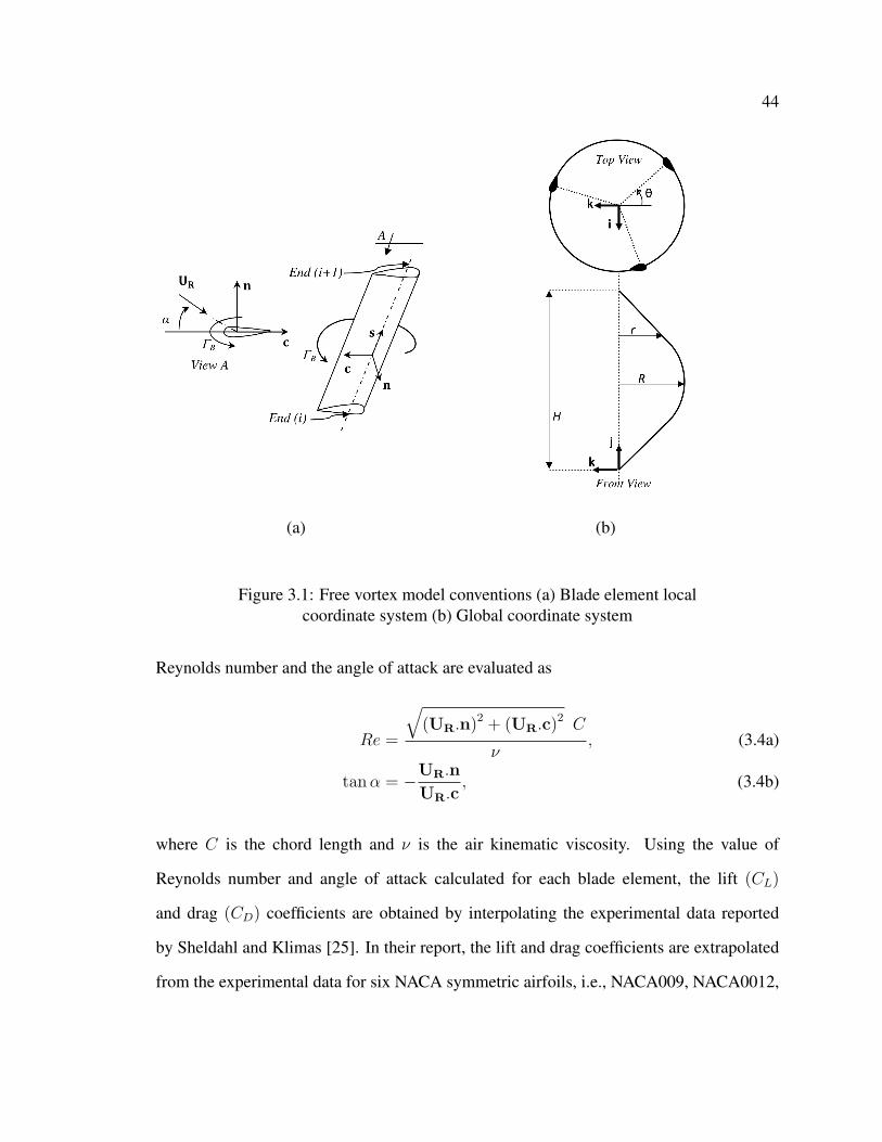
44

(a) (b)

Figure 3.1: Free vortex model conventions (a) Blade element localcoordinate system (b) Global coordinate system

Reynolds number and the angle of attack are evaluated as

Re =

√(UR.n)

2 + (UR.c)2 C

ν, (3.4a)

tanα = −UR.n

UR.c, (3.4b)

where C is the chord length and ν is the air kinematic viscosity. Using the value of

Reynolds number and angle of attack calculated for each blade element, the lift (CL)

and drag (CD) coefficients are obtained by interpolating the experimental data reported

by Sheldahl and Klimas [25]. In their report, the lift and drag coefficients are extrapolated

from the experimental data for six NACA symmetric airfoils, i.e., NACA009, NACA0012,

45

NACA0015, NACA0018, NACA0021 and NACA0025. This information is provided for

the Reynolds number ranges from 104 to 107, and the angle of attack spans from 0 to 180.

The tangential force coefficient CT along the chord and the normal force coefficient CN

normal to the chord are given as

CT = CL sinα− CD cosα, (3.5a)

CN = −CL cosα− CD sinα. (3.5b)

Note that based on the above equations, CT is in the opposite direction of c, i.e., in the

direction of the motion from the trailing edge to the leading edge, and CN is in the di-

rection of the unit vector n. Finally, the strength of the bound vortex per span ΓB, which

replaces each blade element, can be expressed in terms of the lift coefficient using the

Kutta-Joukowski theorem as follows

ΓB =1

2CLC UR. (3.6)

3.2.3 Vortex Shedding

Calculating the strength of the shed vortices, including the spanwise and trailing vortices,

is the next step. The vortices are shed in the form of vortex filaments: spanwise filaments

parallel to the span of the blade element and trailing tip filaments along the chord at both

ends of the blade element. The strength of these filaments are computed according to the

Kelvin and Helmholtz theorems. Based on the Kelvin’s circulation theorem, the bound

vortex strength around a contour enclosing the airfoil and its wake being zero before the

46

start of the motion, must remain zero, i.e.,

dΓB

dt= 0. (3.7)

Due to the fact that the direction of the blade element velocity changes constantly during

one revolution, and the direction of the wind is fixed, the angle of attack that each blade ele-

ment experiences changes periodically. Consequently, the amount of the generated lift and

the bound vortex strength changes accordingly. This change in the bound vortex strength

must be counteracted by a shed spanwise vortex, keeping the change of the total circulation

equal to zero. This means

ΓS = ΓBt − ΓBt+∆t. (3.8)

Fig.3.2 shows the shed spanwise vortex filament from a single blade element over the time.

This figure also shows the trailing tip vortices at both ends of the element. Dictated by

the Helmholtz theorem, the strength of these trailing tip vortex filaments, at both ends of

the element, is equal to the strength of the bound vortex representing each blade element.

Hence the difference between the strength of the bound vortices associated to each blade

element, results in the trailing shed vortices that their strength are given as

ΓT = ΓBi+1− ΓBi

, (3.9)

where ΓBirepresents the bound vortex strength assigned to the blade element i. Note that

at the sections where two blade elements join, these tip vortices do not exist physically;

however, they have to be present numerically to represent the change of the bound vortex

strength along the blade.

47

Figure 3.2: Vortex shedding for a single blade element

3.2.4 Wake Convection

Finally, the last step concerns with the calculation of the distance any point in the fluid

domain travels during the time increment ∆t. Among these points are the start and end

points of the filaments. They convect by the local velocity at that point. An explicit time

integration technique is used to calculate the travelled distance, expressed as

∆x = (1.5Ut − 0.5Ut−∆t + U∞)∆t, (3.10a)

∆y = (1.5Vt − 0.5Vt−∆t)∆t, (3.10b)

∆z = (1.5Wt − 0.5Wt−∆t)∆t, (3.10c)

where, similar to Eq.3.3, U , V and W are the components of the induced velocity in x, y

and z directions. The distance travelled by the vortices that just leave the blade, in their

first time increment, can be calculated as

∆x = (Ut + U∞)∆t, (3.11a)

∆y = Vt∆t, (3.11b)

∆z = Wt∆t. (3.11c)

48

3.2.5 Remarks

In order to complete the aforementioned discussion regarding the free vortex model, it

is worth explaining the approach used for calculating the velocity induced by the vortex

filaments. Moreover, some definitions related to the torque and power of the wind turbine

are presented in the subsequent section.

Induced Velocity

The velocity induced by a vortex filament 〈U, V,W 〉 including bound, spanwise and trailing

vortices, with the strength Γ used in Eq.3.3, is calculated using the Biot-Savart law given

as

〈U, V,W 〉 = Γ

4π

∫l

r× dl

r3, (3.12)

where dl is the incremental length along the vortex filament and r is the position vector

from the incremental length dl to the desired location in the fluid domain. If it is assumed

that the vortex filaments are straight lines, one obtains a more convenient form of the above

equation represented as

〈U, V,W 〉 = Γ

4π

c× a

|c× a|2

(a.b

b− a.c

c

). (3.13)

As shown in Fig.3.3, a extends from the first node to the second node of the vortex filament,

b and c are the vectors that start from the location of interest in the domain and end at the

second and first nodes of the vortex filament respectively.

49

Figure 3.3: Induced velocity at a point by vortex filament

Rotor Performance

In the preceded sections, it was explained how to obtain the tangential (CT ) and normal

(CN) force coefficients. One can easily convert these coefficients to the actual amount of

tangential and normal forces as given by

FT =1

2ρCleCT U2

R, (3.14a)

FN =1

2ρCleCN U2

R, (3.14b)

where le is the length of the blade element. Note that the generated torque can be calcu-

lated as Q = r FT and the generated power as P = ΩQ. Therefore, the non-dimensional

torque (CQ) and power (CP ) coefficients for a single blade is obtained as the sum of these

quantities over the total number of the elements of the blade NE, given as

CQ =NE∑1

r FT

12ρRAFU2

∞, (3.15a)

CP =NE∑1

ΩQ12ρAFU3

∞, (3.15b)

50

where AF is the rotor swept area. It is also common to average the power over one revolu-

tion and define CP as

CP =1

NTI

NTI∑1

CP , (3.16)

where NTI is the number of time increments per revolution of the rotor.

3.3 Numerical Validation

As mentioned earlier, Strickland et al. [9] formulated the aforementioned free vortex

model, and then based upon that, they developed the VDART3 ( Vortex method of so-

lution for the DARrieus Turbine in 3 dimensions) software for the aerodynamic analysis of

VAWTs. The VDART3 code takes non-dimensional parameters as inputs, such parameters

are the chord to radius ratio CR

, the height to radius ratio HR

, the tip speed ratio RΩU∞

, and the

lift and drag coefficients for only one Reynolds number.

In the current investigation, a FORTRAN 90 based software called FEM-Vort is devel-

oped for the aeroelastic analysis of a VAWTs with troposkien shape. The elastic part of the

software is coded using the formulation presented in Chapter 2, and the aerodynamic part

is based on the Strickland free vortex model. Unlike VDART3, FEM-Vort is implemented

based on dimensional input parameters. The reason behind this choice is explained later in

this chapter. Here, to verify the validity of the aerodynamic part of FEM-Vort, the results

generated by this software are compared with the ones reported by Strickland et al. [9] in

the original Sandia report where VDART3 is explained in detail. For the purpose of this

validation, the elastic part of FEM-Vort software is switched off.

The original Sandia report [9] demonstrates the normal and tangential forces generated

at the equator of a two-bladed wind turbine with the following specifications: a chord

51

to equator ratio of CR

= 0.135, a height to radius ratio of HR

= 2, a tip speed ratio of

RΩU∞

= 5, and 5 elements per blade (NE = 5). The lift and drag coefficients used are the

ones for NACA0012 airfoil at the Reynolds number of 0.3× 106. The corresponding input

parameters used in FEM-Vort are as follows: height H = 2m, equator radius R = 1m,

chord length C = 0.135m, the wind turbine angular velocity Ω = 45 rad/s, and the wind

velocity U∞ = 9m/s. The same lift and drag data for the Reynolds number of 0.3× 106 is

also incorporated. This comparison is illustrated in Fig. 3.4.a. The parameters F+T and F+

N

in this figure, which are proportional to the tangential and normal forces, are defined as

F+T = CT

(UR

U∞

)2

and F+N = CN

(UR

U∞

)2

. (3.17a)

Fig.3.4 shows an absolute agreement between the FEM-Vort and VDART3 predictions (F+T

and F+N ). This fulfils the objective of ensuring that the implementation of the free vortex

model in FEM-Vort is error-free.

-0.5

0

0.5

1

1.5

2

2.5

3

0 200 400 600 800 1000 1200 1400 1600 1800

FT+

Azimuth Angle (Deg.)

VDART3 FEM-Vort

(a)

-30

-20

-10

0

10

20

30

0 200 400 600 800 1000 1200 1400 1600 1800

FN+


VDART3 FEM-Vort

(b)

Figure 3.4: Comparison of equator forces between the FEM-Vortaerodynamic and VDART3: chord to equator ratio of C

R= 0.135, height to

radius ratio of HR= 2, tip speed ratio of RΩ

U∞= 5, FEM-Vort with fixed

Reynolds number

52

Due to the lack of a complete set of experimental data in 1980, Strickland et al. [9]

developed VDART3 such that the lift and drag coefficients for all the blade elements are

interpolated using the experimental data at only one Reynolds number regime, the one

that is close to the calculated Reynolds number of the equator of the wind turbine. Since

there was no need to calculate the Reynolds number, the calculation of the absolute value

of velocity was not required. This is the main reason that VDART3 was written in terms

of the non-dimensional parameters mentioned earlier. However, this assumption is not a

reasonable assumption due to the facts that

• Each blade element has a different radius from the vertical axis; hence, it has a dif-

ferent velocity from the other elements.

• The velocity of each blade element changes its direction with the free stream velocity

during one revolution.

Therefore, the magnitude of the relative velocity as well as the Reynolds number changes

not only from one element to the other but also from one position to another. Hence, in

the light of extensive experimental data available now [25], FEM-Vort takes into consider-

ation the variation of the Reynolds number. Consequently, for the sake of calculating the

Reynolds number which demands the absolute value of velocity, FEM-Vort is written for

the dimensional parameters.

Fig.3.5 shows the comparison between VDART3 and FEM-Vort when the variable Reynolds

number effect is included in FEM-Vort. The two results exhibit significant differences when

one compares the tangential force parameter F+T specially at the peaks. This discrepancy

stems from the sensitivity of the lift coefficient to the variation of Reynolds number. To

explore this, let us examine the three graphs presented in Fig.3.6. From Fig.3.6.a, which

shows the variation of angle of attack during five revolutions obtained from FEM-Vort, one

53

can observe that the maximum tangential force happens when the angle of attack is approx-

imately 10. This angle of attack corresponds to a Reynolds number at about 0.48 × 106,

as shown in Fig.3.6.b. Comparing this Reynolds number with the one used in VDART3

(0.3× 106) explains the disparity in the results of FEM-Vort and VDART3. This conclu-

sion will become more evident when one inspects the variation of the lift coefficient with

the Reynolds number in Fig.3.6.c. Implied in this figure, the lift coefficient at the angle

of attack of 10 is very sensitive to the value of the Reynolds number. Conclusively, the

variation of the Reynolds number play an important role in an accurate prediction of the

aerodynamic forces. This effect is taken into account in the development of FEM-Vort.

0

1

2

3

4

0 200 400 600 800 1000 1200 1400 1600 1800

FT+


VDART3 FEM-Vort

(a)

-30

-20

-10

0

10

20

30

0 200 400 600 800 1000 1200 1400 1600 1800

FN+


VDART3 FEM-Vort

(b)

Figure 3.5: Comparison of equator forces between the FEM-Vortaerodynamic and VDART3: chord to equator ratio of C

R= 0.135, height to

radius ratio of HR= 2, tip speed ratio of RΩ

U∞= 5, FEM-Vort with variable

Reynolds number

54

-15

-10

-5

0

5

10

15

0 200 400 600 800 1000 1200 1400 1600 1800

Angle of Attack (Deg.)


(a)

0.3

0.35

0.4

0.45

0.5

0 200 400 600 800 1000 1200 1400 1600 1800

Reynolds Number

× 106


(b)

0

0.2

0.4

0.6

0.8

1

1.2

1.4

0 0.1 0.2 0.3 0.4 0.5 0.6 0.7

Lift Coefficient

Reynolds Number× 106

FEM-Vort Experimental Data VDART3 Experimental Data

(c)

Figure 3.6: The FEM-Vort aerodynamic model: height H = 2m, equatorradius R = 1m, chord length C = 0.135m, the wind turbine angular

velocity Ω = 45 rad/s and the wind velocity U∞ = 9m/s (a) Variation ofangle of attack (b) Variation of Reynolds number (c) Variation of lift

coefficient at AOA = 10 with Reynolds number

55

3.4 Convergence Analysis

In numerical analysis, it is crucial to ensure that the numerical solution most accurately

mimics the physics of the problem by minimizing the influence of the numerical artifacts.

Examples of these numerical artifacts are the ones that might arise from spatial and tem-

poral resolutions. Here, a spatial and temporal convergence analysis is carried out striving

at studying the effect of the number of elements as well as the number of time steps. This

analysis determines the suitable number of elements and time steps for the aeroelastic anal-

ysis which will be presented in the next chapter. The wind turbine chosen for this study is

the 17-meter DOE-Sandia used in the previous chapter. One could refer to reference [26]

for the specifications of this wind turbine.

3.4.1 Spatial Convergence

To ensure the autonomy of the numerical solution from the number of blade elements, the

results obtained from different number of blade elements are compared. One anticipates

that more number of elements leads to a more accurate solution at the expense of higher

computer simulation time; hence, a compromise has to be reached. Fig.3.7.a shows the

tangential force coefficient CT at the equator of the 17-meter DOE-Sandia VAWT with four

different number of blade elements. The results obtained by 23 and 47 elements are almost

identical. Therefore, considering the computer run time restriction, 23 blade elements are

chosen for the rest of the analyses.

3.4.2 Temporal Convergence

Similar to the number of blade elements, a compromise between computer run time and

accuracy has to be reached for selecting the suitable number of time steps. Another factor

56

that plays a role is the fact that very small time step allows high frequency components to

manifest in the aerodynamic forces. Some of these high frequency components not only do

not increase the accuracy of the results but also result in spurious high frequency structural

response.

Fig.3.7.b shows the tangential force coefficient CT at the equator for 20, 40 and 60

time steps per revolution. Evidently, all the results show the same mean trend. The only

difference relies on the fact that 60 time steps introduce high frequency fluctuations in

the solution. In order to decide on the number of time steps, it is insightful to inspect

the Nyquist frequencies associated with each time step. According to the angular velocity

of the wind turbine (50.6 rpm), the Nyquist frequency corresponding to 20, 40 and 60

time steps are 53.25 rad/s, 106.49 rad/s and 159.74 rad/s respectively. These Nyquist

frequencies cover 10, 20 and 30 harmonics. It seems that covering 10 harmonics could be

enough to represent the aerodynamic forces. Hence, considering the computer run time

restriction, 20 time steps per revolution is chosen for the rest of the analyses.

0

0.05

0.1

0.15

0.2

0.25

0.3

0 200 400 600 800 1000 1200 1400 1600 1800

Tangential Force Coefficient

Azimuth Angle (Degree)

5 Elements 11 Elements 23 Elements 47 Elements

(a)

0

0.05

0.1

0.15

0.2

0.25

0.3

0 200 400 600 800 1000 1200 1400 1600 1800



20 Steps/Rev 40 Steps/Rev 60 Steps/Rev

(b)

Figure 3.7: Convergence analysis: 17 meter DOE-Sandia VAWT, the windturbine angular velocity Ω = 50.6 rpm and the wind velocity

U∞ = 22mph (a) Number of blade elements (b) Number of time steps perrevolution

57

3.5 Parallel Implementation

The aerodynamic model presented here provides a more detailed representation of the wake

compared to the momentum based models. This is a significant advantage specially when

aeroelastic analysis demands a more accurate predictions of the aerodynamic forces. How-

ever, from a computational point of view, this model is costly. Although, the computer

run time of this model is considerably less than a full CFD simulation, it is still more

computationally expensive than the momentum based methods. This cost becomes more

pronounced when parametric studies are conducted to investigate the influence of parame-

ters such as geometry and blade shapes. To tackle such problem, a simple parallel version

of the aforementioned model is implemented.

The parallelism implemented herein takes advantage of a shared memory parallel pro-

gramming interface, the so-called OpenMP. The reason for this selection originates from

the physical nature of the free vortex model: according to several computational runs per-

formed in this study, on average, more than 90% of the computation time of this model is

spent on calculating the vortex filament induced velocity at different points in the fluid do-

main. This includes the computation of the velocity at the aerodynamic centres of the blade

sections as well as the start and end points of the other vortex filaments travelling freely in

the wake. In a parallel computation framework, imagine assigning a cluster of vortex fila-

ments named i to the ith CPU of the machine. For calculating the vortex induced velocity

at the nodes of one vortex filament in cluster i, the effect of all other vortex filaments inside

cluster i and inside all other clusters have to be evaluated. This means that for calculating

the induced velocity at one node of one vortex filament, CPU i has to talk to other CPUs

n × m times, where n is the number of clusters and m is the number of vortex filaments

inside each cluster. This value has to be multiplied by m when one considers the total

number of cross talks for all the vortex filaments inside cluster i. This simple calculation

58

shows how massive the cross talks between CPUs could be. This massive communication

between CPUs easily justifies that the implementation of the current vortex model is not

suitable for distributed-memory machines. On the contrary, this model lends itself well to

the shared-memory implementation. This is mainly due to the fact that each CPU takes the

information it requires from a shared memory, accessible to all the CPUs. By using this

approach, the cross-talks between the CPUs are avoided.

The shared memory parallel implementation of the free vortex model is performed using

OpenMP. The routine that calculates the vortex induced velocities consists of four for loops

that are parallelized easily by utilizing the !$OMP DO directive. A case is tested where

the 17-meter DOE-Sandia VAWT completes 10 full revolutions with an angular velocity

of 50.6 rpm. The blades are divided into 23 elements each and 40 time steps are used in

each revolution. The numerical experiments are carried out on a SPARC64 VII machine

that has four 2.4 GHz Quad Core processors with 32 GB RAM and 2 hardware threads

on each core. To ensure that the parallelism is implemented correctly, different quantities

obtained from the parallel implementation were compared against the results of the serial

implementation. As an example of such comparisons, Fig.3.8 illustrates the tangential

force coefficient obtained for the aforementioned case study using 24 CPUs. The exact

match between the two sets of results reveals the validity of the parallel implementation.

Furthermore, Fig.3.9.a shows the computer run time for different number of CPUs. The

serial version takes about five hours to complete; however, as the number of CPUs increases

the run time reduces. Fig.3.9.b shows the scalability graphs in terms of the speed up, where

Speedup = serial run timeparallel run time

. This graph shows that the parallel run scales quite well. The

deviation from the linear scalability could be attributed to the unparallelized part of the

code and hardware restrictions.

59

0

0.05

0.1

0.15

0.2

0.25

0.3

0 200 400 600 800 1000 1200 1400 1600 1800



Serial Implementation Parallel Implementation using 24 CPUs

Figure 3.8: Verification of the parallel implementation in terms of thetangential force coefficient: comparison of the serial and the parallel (using

24 CPUs) implementations, 17 meter DOE-Sandia VAWT, 23 bladeelements, 10 revolutions, 40 steps per revolution

0

1

2

3

4

5

0 5 10 15 20 25

Time (hour)

Number of CPU

(a)

0

5

10

15

20

25

0 5 10 15 20 25

Speedup

Number of CPU

Linear Scalability FEM-Vort Aerodynamic Scalability

(b)

Figure 3.9: Scalability of parallel implementation: 17 meter DOE-SandiaVAWT, 23 blade elements, 10 revolutions, 40 steps per revolution (a)

Computer run time (b) Speedup

3.6 Conclusions

An already developed free vortex model which is based on vortex filaments is adopted in

this chapter with two modifications: the effect of variable Reynolds number is incorporated;

moreover, the most time consuming routine of this model is parallelized using the shared

60

memory parallel programming interface capabilities. The inclusion of the Reynolds num-

ber effect is demonstrated to change the tangential force predictions significantly. It is also

highlighted that the parallel implementation scales well for this application. Furthermore,

in this chapter, the suitable number of blade elements and time steps per revolutions are

chosen through convergence analysis. These requirements will be used in the next chapter

for the aeroelastic analysis of the 17-meter DOE-Sandia VAWT.

Chapter 4

Aeroelastic Analysis

4.1 Introduction

This chapter details the methodology invoked in the aeroelastic analysis of VAWTs. The

aeroelastic analysis is accomplished by coupling the structural dynamic equations, devel-

oped in Chapter 2, with the aerodynamic model, studied in Chapter 3.

The first section of this chapter describes the underlying concepts behind the coupling

formulation. The time integration technique, the so-called average acceleration method,

utilized for evaluating the structural displacement and velocity, is outlined. Then, the ap-

proach taken for updating the aerodynamic loads affected by the structural vibration is

demonstrated.

The second part of this chapter is devoted to the results obtained from the full aeroelastic

simulations of the 17-meter DOE-Sandia VAWT. The aerodynamic performance, including

the predicted aerodynamic torque and the power curve, and the structural performance,

particularly the vibratory stresses, are verified against the experimental data.

61

62

4.2 Aeroelastic Coupling

Typically, in a fluid-structure interaction problem, the loose coupling between the two do-

mains is carried out by following two steps: first the structural responses are evaluated due

to the fluid loads, and then, the structural responses are used as a feedback to the fluid

domain. Here, these two steps are described in more detail.

4.2.1 Structural Deflection

In Chapter 2, it was explained how the tangential (CT ) and normal (CN) force coeffi-

cients are obtained for each blade element. Note that these coefficients are calculated at

the Aerodynamic Centre (AC) located at the quarter chord point from the leading edge. It

is worthwhile pointing out that the moment coefficient is assumed to be zero at AC. This

assumption is particularly true for high Reynolds number regime. There exist small aerody-

namic moments at relatively smaller Reynolds number, which is assumed to be negligible

in this analysis.

In order to apply the tangential and normal aerodynamic forces on the structure, these

forces have to be moved to the Elastic Axis (EA) of the structure. To perform this, a moment

has to be applied at EA, as illustrated in Fig.4.1.a. The non-dimensional magnitude of this

moment is CM = CNd0

b, where d0

bis the non-dimensional distance between EA and AC

with respect to the half chord length b. Referring to these coefficients, one can find the

distributed forces T and N , and the distributed moment M over the the blade element as

T =1

2ρCCT U2

R, (4.1a)

N =1

2ρCCN U2

R, (4.1b)

M =1

2ρbCCM U2

R, (4.1c)

63

where UR is the blade velocity superimposed by the wind and vortex induced velocities. It

is assumed that these forces are evenly distributed over the aerodynamic blade element.

An accurate prediction of the structural vibration demands sufficient number of FEM

elements. This number of FEM elements are typically greater than the ones needed for the

aerodynamic model. Therefore, each aerodynamic blade element might constitute of one to

several FEM elements. The aerodynamic load distribution calculated for any aerodynamic

blade element in Eq.4.1, could be attributed to the FEM elements belong to it. Hence,

depending on the length of the FEM element, one could easily assign half of the distribution

to each node of the FEM element, representing the FEM nodal forces. Referring to the

rotating frame of reference shown in Fig.4.1.b, N and T are aligned along e1 and e2, and

M is about e3. However, the signs have to be decided based on the directions of the frame

of reference axes.

(a) (b)

Figure 4.1: (a) Aerodynamic forces on the blade section (b) Rotating frameof reference

64

Once the aerodynamic forces are properly incorporated in the right hand side of the

following structural dynamic equation,

M ÿD + C ˙yD +KyD = F, (4.2)

this equation is solved in time. The time integration technique used in this analysis is the

so-called average acceleration method. This technique is an implicit scheme and uncondi-

tionally stable. The steps are as follows:

Algorithm: Average Acceleration Method

inputs: initial displacement yD0, initial velocity ˙yD0

1 compute: initial acceleration ÿD0 = M−1(F0 − C ˙yD0 −KyD0

)2 for i = 1, 2, ..., na: total number of aerodynamic updates

3 for j = 1, 2, ..., ns: number of structural calculations between two aerodynamic updates

4 k = (i− 1)ns + j

5 compute: yDk+1 =[

4h2 M + 2

hC +K

]−1 (Fi+1 +M

(4h2 yDk + 4

h˙yDk + ÿDk

)+ C

(2hyDk + ˙yDk

))6 compute: ˙yDk+1 = − ˙yDk + 2

h(yDk+1 − yDk)

7 compute: ÿDk+1 = −ÿDk + 4h2

(yDk+1 − yDk − h ˙yDk

)8 end for

9 end for

In this algorithm, h is the time step for the structural calculation. Since the computer run

time for the structural calculation is significantly less than the aerodynamic calculation, the

average acceleration method is implemented such that several structural calculations can

65

be performed between the two aerodynamic updates. Of course, for each set of these cal-

culations, the aerodynamic forces are assumed to be unchanged, having the most updated

value.

4.2.2 Aerodynamic Updates

Following the structural vibration, the aerodynamic forces have to be adapted such that

they account for this vibration. With regards to the aerodynamic formulation presented in

Chapter 2, two adjustments seem to be necessary to impose on the fluid domain:

• In Chapter 3, the Aerodynamic Centre (AC) of each section of the blade was assumed

to travel the perimeter of a full circle. This is a true assumption when the structure is

considered to be rigid. However, flexibility of the structure violates this assumption

in a sense that the deformation of the structure causes AC to deviate from a circular

path.

• Vibration induced velocities have to be also superimposed on the blade, free stream

and the vortex induced velocities.

For a full aeroelastic simulation these effects have to be taken into account. A more detailed

discussion is presented next.

Structural Displacement

In Chapter 3, the blades were assumed to be rigid. Hence, the location of the aerodynamic

centre (AC) of any blade section was dictated by the equation of a circle, as follows

66

θB =2π

NB(BN − 1) + θ, (4.3a)

X = −r sin θB, (4.3b)

Z = −r cos θB, (4.3c)

where 〈X,Y, Z〉 is the global coordinates of AC of any section of the blades, and θB is the

blade azimuth angle.

Assuming a more realistic case, where the blades are flexible, allows AC of the blade

section to vibrate about the rigid body position. Although this deflection is relatively small

compared to the rigid body motion, it has to be considered in an aeroelastic analysis. Note

that the structural displacement yD obtained as the output of the average acceleration

method at each time step, are the displacements of the Elastic Axis (EA) in the rotating

frame of reference depicted in Fig.2.1.a. Hence, one has to relate the movements of AC to

the EA displacements. Moreover, because the motion of the blades and the vortices in the

aerodynamic model are tracked in a stationary coordinate system shown in Fig.3.1.b, the

displacements of AC has to be transformed into this coordinate system. The details of this

process is discussed in the second section of Appendix A. Based on that, Eq.4.3 has to be

updated for the structural displacement as follows

θB =2π

NB(BN − 1) + θ, (4.4a)

X = −r sin θB +∆X, (4.4b)

Z = −r cos θB +∆Z, (4.4c)

and ∆Y has to be added to the values obtained from the troposkien geometry. ∆X , ∆Y ,

67

∆Z are defined as

∆X = m sin θB − v cos θB, (4.5a)

∆Y = n, (4.5b)

∆Z = m cos θB − v sin θB, (4.5c)

where

m =(d0χ1 − w

)cosφ+

(u+ d0α

)sinφ,

n =(u− d0α

)cosφ+

(d0χ1 − w

)sinφ,

and yD = uχ1 v χ2wαT is the displacement of the elastic axis, and φ is shown in

Fig.4.1.b.

Now that the location of the AC points are updated due to the structural displacement, let

us revisit the local coordinate system previously defined for rigid blades in Section 3.2.1,

i.e.,


2 + (Yi+1 − Yi)2 + (Zi+1 − Zi)

2, (4.6a)

c = cos θBi− sin θBk, (4.6b)

n = s× c, (4.6c)

where 〈Xi, Yi, Zi〉 is ithe AC along the blade. Note that updating the coordinates of the

aerodynamic centre due to structural deflection, as described earlier, automatically revises

the vector s. Besides s, the vector c, which represents the chordwise direction of the blade

section, has to also account for the structural deflection. This is explained in the third

68

section of Appendix A in detail. Based on the results, Eq.4.6 has to be updated as given by


2 + (Yi+1 − Yi)2 + (Zi+1 − Zi)

2, (4.7a)

c = cos θBi− sin θBk+∆c, (4.7b)

n = s× c, (4.7c)

where ∆c is defined as

∆c =

− (α sinφ+ χ1 cosφ) sin θB

α cosφ− χ1 sinφ

− (α sinφ+ χ1 cosφ) cos θB

. (4.8)

Structural Velocities

In Chapter 3, the following equation was used to calculate the velocities of AC of any

section of the rigid blade

UR = (U + U∞ + Ut cos θB) i+ V j+ (W − Ut sin θB)k, (4.9)

where Ut is the blade rotational velocity, U∞ is the free stream velocity and 〈U, V,W 〉

is the induced velocity caused by the vortices. However, for the aeroelastic analysis the

vibration induced velocity has to be added to this equation. In the previous sections, it was

shown how solving the structural dynamic equation could result in evaluating the structural

velocity ˙yD at the elastic axis. In order to exploit this velocity in the aerodynamic model,

they have to be transformed to the aerodynamic centre of the blade section, with respect to

69

the 〈i, j,k〉 coordinate. The required equations are derived in the last section of Appendix

A. Referring to these equations, Eq.4.9 has to be updated as follows

UR =(U + U∞ + Ut cos θB + X

)i+

(V + Y

)j+

(W − Ut sin θB + Z

)k, (4.10)

where

X = (m− Ωv) sin θB − (v − Ω (m+ r)) cos θB, (4.11a)

Y = n, (4.11b)

Z = (m− Ωm) cos θB − (v − Ω (v − r)) sin θB, (4.11c)

m and n are defined as

m =(d0χ1 − w

)cosφ+

(u+ d0α

)sinφ,

n =(u− d0α

)cosφ+

(d0χ1 − w

)sinφ,

and yD = u χ1 v χ2 w αT is the velocity of the elastic axis of the blade section.

4.3 Results and Discussions

Here, the aeroelastic results of FEM-Vort for the analysis of 17-meter DOE-Sandia VAWT

is presented. Aerodynamic performance of this VAWT is discussed in terms of the gen-

erated torque and power curve. Furthermore, the structural performance is demonstrated

through the structural parameters such as displacement, internal forces, strain and stress.

70

4.3.1 Aerodynamic Performance

Aerodynamic Torque

Fig.4.2 illustrates the comparison of FEM-Vort torque predictions with the experimental

data. The experimental data is obtained from the measurements performed by McNerney

[27] on the 17-meter DOE-Sandia VAWT. Shown in this figure, at the relatively high Tip

Speed Ratio (TSR), i.e., high ratio of the blade velocity at the equator to the wind velocity,

in this case 4.36, the agreement between FEM-Vort and the experimental data is excellent.

However, for the lower values of TSR, FEM-Vort demonstrates poor predictions. This

is implied at TSR = 2.8 and TSR = 2.18. Berg [28] reports that this mainly hinges

on the dynamic stall phenomenon: At relatively high tip speed ratio, due to the higher

magnitude of the blade velocity, the relative velocity creates a smaller angle with the blade

velocity. Therefore, the angle of attack becomes lower. For a typical TSR of 4 or greater,

the angle of attack of the equator and the sections close to it, vary in a range which is less

than the static stall angle of attack. Note that the sections close to the equator are mostly

responsible for generating the torque due to the higher radius (arm). Hence, dynamic stall

does not play a crucial role. However, at the lower tip speed ratios, such as 2.8 and 2.18, the

maximum angle of attack of the equator exceeds the static stall angle. Therefore, the blade

periodically transitions between the stalled and unstalled conditions. This fact unfolds the

necessity for including the dynamic stall model in FEM-Vort. Berg [28] incorporates a

modified Boeing-Vertol dynamic stall model into VDART3 and shows that the results for

the torque predictions improve significantly.

71

-10

0

10

20

30

40

0 50 100 150 200 250 300 350

Torque (kN.m)


FEM-Vort Experimental Data

Experimental Error Bound

(a)

-10

0

10

20

30

40

0 50 100 150 200 250 300 350

Torque (kN.m)




(b)

-10

0

10

20

30

40

0 50 100 150 200 250 300 350

Torque (kN.m)




(c)

Figure 4.2: Comparison of the generated torque: 17-meter DOE-SandiaVAWT, operating angular velocity Ω = 50.6 rpm (a) Tip speed ratio = 2.18

(b) Tip speed ratio = 2.8 (c) Tip speed ratio = 4.36

72

Power Curve

Fig.4.3 presents the power curve predicted by FEM-Vort for the 17-meter DOE-Sandia

VAWT at the operating angular velocity of 50.6 rpm. The experimental data, obtained

from the reference [10], is also plotted. Although the trend of the experimental data is

predicted reasonably, there exists an offset between the values. At low tip speed ratio, this

offset is mainly due to the lack of dynamic stall model in the calculations as discussed

earlier. However, the discrepancies exist at high tip speed ratios have to be investigated

further.

0

0.1

0.2

0.3

0.4

0.5

0 2 4 6 8 10 12

Power Coefficient

Tip to Wind Speed Ratio


Figure 4.3: The power curve of the DOE-Sandia 17 meter VAWT:operating angular velocity Ω = 50.6 rpm

Wake Structure

Fig.4.4 shows the wake structure of the 17-meter DOE-Sandia VAWT when the azimuth

angle θ becomes 1890 or 90 after completing five revolutions. At this position, the chord-

wise axis of the blades are perpendicular to the direction of the wind. The upwind blade

generates maximum torque while the generated torque by the downwind blade is damped

out due to the strong interaction with the vortices. In Fig.4.4, the colours assigned to the

vortices are chosen based on their evolution in time. The vortices with the blue colour left

73

the blades initially, while, the red colour vortices have just initiated their movements. The

points shown here as the vortices belong to the start and end nodes of the vortex filaments

when convecting downstream of the wind turbine. This figure implies that the movement

of the vortices at the core is delayed by the strong interaction with the other vortices.

Figure 4.4: Wake structure: 17-meter DOE-Sandia VAWT, operatingangular velocity Ω = 50.6 rpm, tip speed ratio = 4.36, azimuth angle

(θ) = 1890

4.3.2 Structural Performance

Structural Displacement

The Elastic Axis (EA) displacements of the 17-meter DOE-Sandia VAWT at the equator

are shown in Fig.4.5. Due to the symmetry of the structure with respect to the equator and

the lack of gravitational forces in the model, the plunge (χ1) and chordwise (χ2) rotational

displacements as well as the spanwise translational displacement (w) are zero. Fig.4.5

shows that the maximum steady-state amplitudes of the plunge (u), chordwise (v) and

74

pitch (α) displacements are 25mm, 7.5mm and 0.08 respectively. The relatively small

magnitude of these degrees of freedom proves that the effect of the structural displacements

in changing the aerodynamic forces is minimal.

Fig.4.6 presents the frequency content of the aforementioned displacements. The DC

term of the frequency content of u exhibits a value of about 25mm. This is the mean value

of the plunge displacement evident in Fig.4.5.a as well. The main cause of this relatively

large mean value is the steady-state centrifugal force manifest itself in vector fss in Eq.2.19.

The vibratory part of this displacement comes from the aerodynamic forces, representing

the non-zero frequency components. The zero-frequency term for v is 2.5mm approxi-

mately. Since the centre of mass offset is assumed to be zero in this analysis, i.e., xα = 0,

the chordwise component of the centrifugal force fss is zero as well. Hence the response

v is purely aerodynamic dependent. The mean offset of v conforms with the fact that the

tangential force and consequently the generated torque depicted in Fig.4.2 oscillates about

a non-zero mean. Moreover, it is noticeable that the other dominant frequency components

of v response are the first four harmonics, i.e., Ω, 2Ω, 3Ω and 4Ω, where Ω is the angular

velocity of wind turbine, in this case 5.3 rad/s. Similarly, these harmonics are also present

in the frequency content of the pitch displacement α, shown in Fig.4.6.b. Note that the

mean value of α is a response to only aerodynamic forces because the centrifugal spanwise

moment f6ss = −bxαr sinφ is zero.

It is worthwhile pointing out that herein, the initial displacement yD0 and velocity ˙yD0,

required in the calculation of the Average Acceleration Method, are assumed to be zero.

The influence of such an assumption is evident in the transient response of the system

shown in Fig.4.7. According to this figure, the transient response disappears after almost

two revolutions of the wind turbine. This is due to the structural damping mechanism intro-

duced to the system. The structural damping used in this analysis is a stiffness proportional

75

damping that introduces 5% damping to the 10th natural frequency of the system. This

means that the first to the 9th natural frequencies experience less than 5%; conversely, the

rest experience more than 5% damping. This type of damping guarantees that the solution

is not smeared by any spurious high frequency component.

-40

-35

-30

-25

-20

-15

-10

-5

0

5

0 500 1000 1500 2000 2500 3000 3500

Translational Displacement (mm)


Plunge Chordwise Spanwise

(a)

-0.15

-0.1

-0.05

0

0.05

0.1

0.15

0 500 1000 1500 2000 2500 3000 3500

Rotational Displacement (Deg.)


Plunge Chordwise

Pitch

(b)

Figure 4.5: Elastic axis displacement at the equator of the 17-meterDOE-Sandia VAWT: operating angular velocity Ω = 50.6 rpm,

tip speed ratio = 4.36 (a) Translational displacement (b) Rotationaldisplacement

0

5

10

15

20

25

0 10 20 30 40 50

Displacement (mm)

Frequency (rad/s)

Plunge Chordwise

(a)

0

0.005

0.01

0.015

0.02

0.025

0.03

0.035

0.04

0 10 20 30 40 50

Pitch Displacement (Deg.)

Frequency (rad/s)

(b)

Figure 4.6: Frequency content of the elastic axis displacement at theequator of the 17-meter DOE-Sandia VAWT: operating angular velocityΩ = 50.6 rpm, tip speed ratio = 4.36 (a) Translational displacement (b)

Pitch displacement

76

Internal Forces

One of the advantages of the mixed finite element formulation presented in Chapter 2 relies

on the fact that following the calculation of the generalized displacement vector yD =

uχ1 v χ2wαT from Eq.2.23, the generalized force vector yF = Q1M1Q2M2 τ M3T

could easily be evaluated by using the system of equations presented in Eq.2.16, i.e.,

yF = −K−1FFKFDyD. (4.12)

Fig.4.7 illustrates the internal forces at the root of the 17-meter DOE-Sandia VAWT,

namely the moment about the plunge axis M1, the moment about the chordwise axis M2

and the axial force τ . Two sets of results are plotted: the response to the complete set

of external forces, i.e., aerodynamic and centrifugal forces, and the response to only the

centrifugal forces. Referring to Fig.4.7.a, M1 only consists of the response of the structure

to the aerodynamic loading. On the contrary, the internal moment M2 is combination of

the mean value that arises from the centrifugal force and a vibratory part that comes from

the aerodynamic load fluctuations. Likewise, τ is developed due to both aerodynamic and

centrifugal forces.

Strain & Stress

The cyclic nature of the aerodynamic loading underscores the necessity of the fatigue anal-

ysis for the VAWTs’ blade. To carry out such an analysis, Veers [5] highlights that the

time history of the axial stress is the most important factor to consider. Hence, the focus of

this section is to predict the time history of the axial strain and stress. These quantities are

found for the 17-meter DOE-Sandia VAWT.

77

-6

-4

-2

0

2

4

6

8

0 500 1000 1500 2000 2500 3000 3500

Moment about Plunge Axis (kN.m)


Only Centrifugal Centrifugal+Aerodynamic

(a)

-6

-4

-2

0

2

4

6

8

0 500 1000 1500 2000 2500 3000 3500

Moment about Chordwise Axis (kN.m)



(b)

30

35

40

45

50

55

60

65

70

0 500 1000 1500 2000 2500 3000 3500

Axial Force (kN)



(c)

Figure 4.7: Elastic axis internal forces at the root of the 17-meterDOE-Sandia VAWT: operating angular velocity Ω = 50.6 rpm,

tip speed ratio = 4.36 (a) Moment about plunge axis (b) Moment aboutchordwise axis (c) Axial force

78

For calculating the axial strain and stress, the following equation is exploited, assuming

that the neutral centre coincides with the elastic axis,

εss =τ

EA− M1x

EIyy+

M2y

EIxx, (4.13a)

σss = Eεss, (4.13b)

where (ye1 + xe2) is the location of any desired point on the blade section. The axial strain

at the root of the blade is illustrated in Fig.4.8 for two locations: elastic axis and the trailing

edge. The mean offset of the axial strain at the elastic axis is caused by the steady centrifu-

gal force, and the vibratory part by the aerodynamic forces. The same trend happens for

the axial strain at the trailing edge except that the response is amplified by the presence of

the moment M1. Fig.4.9 reveals the same behaviour for the stress.

50

100

150

200

0 500 1000 1500 2000 2500 3000 3500

Axial Microstrain


(a)

50

100

150

200

0 500 1000 1500 2000 2500 3000 3500

Axial Microstrain


(b)

Figure 4.8: Axial strain at the root of the 17-meter DOE-Sandia VAWT:operating angular velocity Ω = 50.6 rpm,

tip speed ratio = 4.36 (a) Elastic axis (b) Trailing edge

79

2

4

6

8

10

12

14

16

0 500 1000 1500 2000 2500 3000 3500

Axial Stress (MPa)


(a)

2

4

6

8

10

12

14

16

0 500 1000 1500 2000 2500 3000 3500

Axial Stress (MPa)


(b)

Figure 4.9: Axial stress at the root of the 17-meter DOE-Sandia VAWT:operating angular velocity Ω = 50.6 rpm,

tip speed ratio = 4.36 (a) Elastic axis (b) Trailing edge

Fig.4.10 demonstrates the elastic axis axial stress along the blades of the 17-meter DOE-

Sandia VAWT. This snapshot is taken at the azimuth angle (θ) of 1890 or 90 after com-

pleting five revolutions. At this position, the elastic axis axial stress at the root of the

upwind blade is at its peak. This is evident in Fig.4.9.a as well. Fig.4.10 reveals the fact

that the roots of the blades experience higher stress comparing to the equator. This figure

also demonstrates that the blades are at higher level of stress when they are in the upwind

position. This is mainly due to the higher amount of aerodynamic forces at the upwind

position when compared to the downwind position.

80

Figure 4.10: Elastic axis axial stress along the blades of the 17-meterDOE-Sandia VAWT: operating angular velocity Ω = 50.6 rpm,

tip speed ratio = 4.36, azimuth angle (θ) = 1890

Finally, Fig.4.11 shows the trailing edge vibratory stress at the root of the 17-meter

DOE-Sandia VAWT at different wind speed. In this figure, the results estimated by FEM-

Vort are compared with the experimental data reported by Lobitz [12]. The vibratory

stresses are taken to be half of the difference between maximum and minimum stresses. Im-

plied in the definition of the vibratory stress, the effect of the steady state centrifugal forces

are eliminated. Hence, the vibratory stress is merely linked to the aerodynamic oscillatory

effects. Fig.4.11 illustrates a very good agreement between the FEM-Vort predictions and

the experimental data when the tip speed ratio is relatively high, namely greater than 2.5.

This range of tip speed ratios corresponds to the wind speeds less than 35mph for the oper-

ating angular velocity of 50.6 rpm. At low tip speed ratios, when the wind speed is higher

than 35mph, the numerical model developed here exhibits limited success in estimating

the correct values of the vibratory stresses. This major limitation stems from inaccurate

prediction of the aerodynamic loading at low tip speed ratios. As discussed earlier, this is

mainly due to the absence of the dynamic stall model.

81

0

1000

2000

3000

4000

5000

6000

7000

0 10 20 30 40 50 60

Vibratory Stress (PSI)

Wind Speed (MPH)


Figure 4.11: Trailing edge vibratory stress at the root of the DOE-Sandia17-meter VAWT: operating angular velocity Ω = 50.6 rpm

4.4 Conclusions

The specially devised structural dynamic equations for curved blades with troposkien shapes

are coupled with the free vortex aerodynamic model. The accuracy of the aeroelastic model

in predicting the aerodynamic performance is illustrated through torque and power esti-

mations. It is shown that the model developed here is able to estimate the aerodynamic

loads reasonably well except where the tip speed ratios are relatively low. This is mainly

attributed to the lack of dynamic stall model in the current investigation. The same defi-

ciency carries over when the numerically evaluated vibratory stresses are assessed. Except

the region of the low tip speed ratios, this analysis provides a very good predictions of the

stress in the blades of a VAWT.

Chapter 5

Conclusions and Recommendations

5.1 Summary

A set of structural dynamic equations which describes the behaviour of a troposkien shape

blade is treated in the finite element framework. The already developed structural dynamic

equations were cast in the form of 12 first order ordinary differential equations in terms

of generalized displacement and generalized force. The nature of the equations enforces

a mixed finite element formulation derivation. This formulation is verified through modal

analysis by inspecting the variation of the natural frequencies with respect to the angular

velocity of the turbine. It is highlighted that the centrifugal stiffening effect prevents the

system from dynamic instability. Furthermore, the effect of centre of mass offset and the

Coriolis forces on the mode shapes of the structure are explored. These effects give rise to

the coupling between certain degrees of freedom of the system. This system is assumed to

vibrate in response to oscillating aerodynamic forces, hence it was required to incorporate

an aerodynamic model.

A three dimensional free vortex model based on vortex filaments, already developed

82

83

for VAWTs, is implemented. The effect of variable Reynolds number is augmented to

the model. This feature alters the tangential force predictions substantially. Comparison

between the predictions of this model and the experimental data reveals the capability of

this model in estimating the aerodynamic forces especially for high tip speed ratios, where

blade-vortex interaction becomes strong. However, the low tip speed ratios do not exhibit a

good agreement mainly because dynamic stall is not considered in this aerodynamic model.

Moreover, a simple parallel implementation of this model is shown to scale well with the

increase of number of CPUs.

The two aforementioned models are coupled to form an aeroelastic model. This is car-

ried out by calculating the structural responses to the aerodynamic and centrifugal forces

in time using the average acceleration method. Then, the structural displacements and

velocities are used to update the aerodynamic loading. Having developed this aeroelastic

capability, the axial stresses along the blade are computed. The comparison of the vibratory

stresses obtained from the analysis of the 17-meter DOE-Sandia VAWT with the experi-

mental data shows an excellent agreement except where dynamic stall plays an important

role.

5.2 Conclusion

The conclusion of the current thesis is summarized as following:

• The coupling between the linear structural dynamic equations developed by Nitzsche

[16] and the vortex filament based aerodynamic model devised by Strickland [9] pro-

vides a robust tool for investigating the aeroelastic behaviour of a VAWT in relatively

high tip speed ratios.

• For providing reasonable estimation in low tip speed ratios, a suitable dynamic stall

84

model has to be added to this model.

• This model lends itself well to shared memory based parallel implementation.

5.3 Recommendations and Future Work

Recommendations for improving the structural analysis:

• The current investigation neglects the effect of gravitational forces. As opposed to

the centrifugal and aerodynamic loading, gravitational forces are unsymmetric with

respect to the equator of the wind turbine. It is interesting to investigate the effect

of this type of unsymmetric loading on the response of the structure, in combination

with the aerodynamic and centrifugal forces.

• The structural dynamic equations used in this analysis are linear. Therefore, it will

be very insightful to study the effect of geometric non-linearity in this problem. This

becomes very important when the study of large deflections in more flexible blades

is of interest.

Recommendations for improving the aerodynamic analysis:

• As emphasized throughout the thesis, the absence of dynamic stall model degraded

the accuracy of the numerical predictions in low tip speed ratio regimes. Including a

suitable dynamic stall model could enhance the results significantly. A wide range of

dynamic stall models are available, ranging from CFD based models to pure empiri-

cal ones. For instance ONERA model is a semi-empirical dynamic stall model, which

is very popular in helicopter applications. Perhaps applying the ONERA model could

shed some light in understanding the dynamic stall mechanism in VAWTs.

85

• In the current study, the wind velocity is assumed to be uniformly distributed along

the height of the wind turbine. A more realistic case of study takes into account

the atmospheric boundary layer effect. In the atmospheric boundary layer, the wind

is generally gusty or turbulent, with the wind changing speed and direction rapidly.

Considering this effect leads to more accurate predictions of the wind turbine perfor-

mance.

• As a long term goal, it would be very compelling to replace the use of experimental

data with a CFD based solution. The flow very close to the airfoil could be solved

using CFD approaches and then the solution could be transferred to a vortex based

approach in the wake of the airfoil. Although this coupled approach becomes com-

putationally expensive, it would provide better resolution to the solution.

Future work for extending the application:

• The developed aeroelastic model showed promising results for the analysis of land-

based VAWTs. This work could be extended for analyzing the behaviour of offshore

VAWTs by implementing the effect of hydrodynamic forces in the base of the wind

turbine.

• One of the disadvantages of VAWTs compared to HAWTs is the fatigue-related prob-

lems due to cyclic aerodynamic loading. The current model gives the opportunity for

performing fatigue analysis by providing the time history of stress. Hence, a po-

tential option for extending the current research is to use the predicted stresses for

estimating the fatigue life of the blades.

• The current method of analysis is a relatively simple and robust tool for investigating

the wind farm effects on the performance of individual wind turbines.

Appendix A

Appendix A: Aerodynamic Updates due

to the Structural Vibration

A.1 Coordinate Systems and Transformation Matrices

For the sake of a more convenient discussion in the following sections, four coordinate

systems are defined here. The definitions of these coordinate systems, which are shown in

Fig.A.1, are as follows:

• i, j, k: the origin of this stationary coordinate system is placed at the bottom of the

wind turbine.

i: is in the direction of the wind.

j: is in the direction of the vertical axis from the bottom to the top.

k: k = i× j.

• er, eθ, eζ : the origin of this rotating coordinate system is placed at intersection of

the local radius r, and the vertical axis of the turbine. This system rotates with the

turbine’s angular velocity Ω.

86

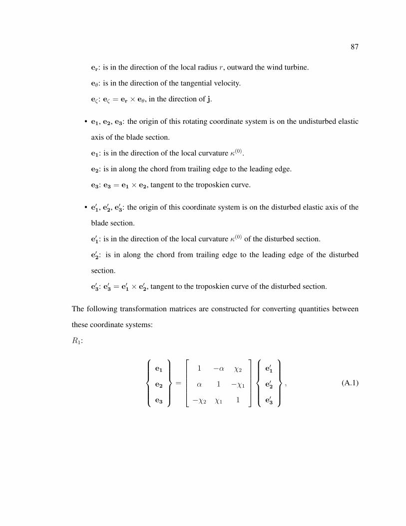
87

er: is in the direction of the local radius r, outward the wind turbine.

eθ: is in the direction of the tangential velocity.

eζ : eζ = er × eθ, in the direction of j.

• e1, e2, e3: the origin of this rotating coordinate system is on the undisturbed elastic

axis of the blade section.

e1: is in the direction of the local curvature κ(0).

e2: is in along the chord from trailing edge to the leading edge.

e3: e3 = e1 × e2, tangent to the troposkien curve.

• e′1, e′2, e′3: the origin of this coordinate system is on the disturbed elastic axis of the

blade section.

e′1: is in the direction of the local curvature κ(0) of the disturbed section.

e′2: is in along the chord from trailing edge to the leading edge of the disturbed

section.

e′3: e′3 = e′1 × e′2, tangent to the troposkien curve of the disturbed section.

The following transformation matrices are constructed for converting quantities between

these coordinate systems:

R1:

e1

e2

e3

=

1 −α χ2

α 1 −χ1

−χ2 χ1 1

e′1

e′2

e′3

, (A.1)

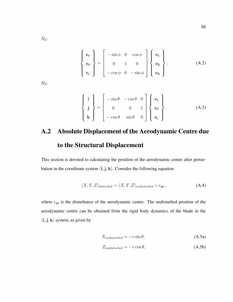
88

R2:

er

eθ

eζ

=

− sinφ 0 cosφ

0 1 0

− cosφ 0 − sinφ

e1

e2

e3

, (A.2)

R3:

i

j

k

=

− sin θ − cos θ 0

0 0 1

− cos θ sin θ 0

er

eθ

eζ

. (A.3)

A.2 Absolute Displacement of the Aerodynamic Centre due

to the Structural Displacement

This section is devoted to calculating the position of the aerodynamic centre after pertur-

bation in the coordinate system 〈i, j,k〉. Consider the following equation

〈X,Y, Z〉disturbed = 〈X, Y, Z〉undisturbed + εac, (A.4)

where εac is the disturbance of the aerodynamic centre. The undisturbed position of the

aerodynamic centre can be obtained from the rigid body dynamics of the blade in the

〈i, j,k〉 system, as given by

Xundisturbed = −r sin θ, (A.5a)

Zundisturbed = −r cos θ, (A.5b)

89

where Yundisturbed could be calculated from the troposkien geometry. Now, let us focus on

calculating εac:

As shown in Fig.A.1.b, the distance between the elastic axis and the aerodynamic centre

before the vibration is d0 = d0e2, in the 〈e1, e2, e3〉 coordinate system. Assume that the

magnitude of d0 will be unchanged during the perturbation and it only undergoes pure

rotation, denoted by d after perturbation. Using the transformation matrix R1, one can find

d in the 〈e1, e2, e3〉 coordinate system, as given by

d = RT1 d0 = d0 (αe1 + e2 − χ1e3) . (A.6)

Referring to Fig.A.1.b, the disturbed position of the aerodynamic centre with respect to the

undisturbed elastic axis, ρ, could be obtained as

ρ = εea + d =(u+ d0α

)e1 +

(v + d0

)e2 +

(w − d0χ1

)e3, (A.7)

where εea is the disturbance of the elastic axis. On the other hand, one can write the

disturbance of the aerodynamic centre (εac) as follows

εac = ρ− d0 =(u+ d0α

)e1 + (v) e2 +

(w − d0χ1

)e3. (A.8)

Note that Eq.A.8 shows the disturbance of the aerodynamic centre in the rotating coordi-

nate system 〈e1, e2, e3〉. In order to update the locations of AC in the aerodynamic model,

one has to represent this equation in the stationary coordinate system 〈i, j,k〉. To perform

this, the transformation matrices R2 and R3 have to be multiplied by εac, i.e, R3R2εac. This

90

manipulation results in the following equation

εac =

∆X

∆Y

∆Z

=

m sin θ − v cos θ

n

m cos θ − v sin θ

, (A.9)

where

m =(d0χ1 − w

)cosφ+

(u+ d0α

)sinφ,

n =(u− d0α

)cosφ+

(d0χ1 − w

)sinφ.

A.3 Rotation of the Blade Section due to the Structural

Displacement

As described in the previous section, the chordwise axis of the blade undergoes only pure

rotation due to the structural vibration, i.e., d = d0. This is an important aspect to be con-

sidered when aerodynamic forces are being calculated. Referring to the previous section,

the unit vector of this rotation vector could be calculated as

c = −d

d= −αe1 − e2 + χ1e3. (A.10)

Note that Eq.A.10 is expressed in terms of 〈e1, e2, e3〉, and it has to be transformed into

the stationary coordinate system 〈i, j,k〉. To conduct this, the transformation matrices R2

91

and R3 have to be used, the result is

c = −R3R2d

d=

cos θ − (α sinφ+ χ1 cosφ) sin θ

α cosφ− χ1 sinφ

− sin θ − (α sinφ+ χ1 cosφ) cos θ

. (A.11)

A.4 Absolute Velocity of the Aerodynamic Centre due to

the Structural Velocity

This section aims at calculating the absolute velocity of the aerodynamic centre in the

coordinate system 〈i, j,k〉. The following well-known equation is used for this purpose

〈X, Y , Z〉 = r+ εac +Ω× εac. (A.12)

Note that the first term, r, can easily be expressed as r = −rΩeθ. One can transform r into

the 〈i, j,k〉 system by multiplying it with R3, i.e.,

r = rΩ (cos θi− sin θk) . (A.13)

Furthermore, the second term of Eq.A.12, εac, could be calculated by taking the derivative

of Eq.A.9 in time,

εac =

m sin θ − v cos θ

n

m cos θ − v sin θ

, (A.14)

92

where

m =(d0χ1 − w

)cosφ+

(u+ d0α

)sinφ,

n =(u− d0α

)cosφ+

(d0χ1 − w

)sinφ.

Finally, since Ω can be written as Ω = Ωj, the last term of term of Eq.A.12, Ω× εac, is

obtained as

Ωj× εac =

Ω (m cos θ − v sin θ)

0

−Ω (m cos θ − v sin θ)

. (A.15)

The aforementioned manipulations result in the final equation for the absolute velocity of

the aerodynamic centre in the coordinate system 〈i, j,k〉, given as

X

Y

Z

=

(m− Ωv) sin θ − (v − Ω (m+ r)) cos θ

n

(m− Ωm) cos θ − (v − Ω (v − r)) sin θ

. (A.16)

93

(a) (b)

Figure A.1: (a) Coordinate systems (b) Blade section displacement

Bibliography

[1] Thomas D Ashwill, Herbert J Sutherland, and Dale E Berg. A retrospective of VAWTtechnology. Technical report, Sandia National Laboratories, 2012.

[2] Walter Musial and Bonnie Ram. Large-scale offshore wind power in the UnitedStates: Assessment of opportunities and barriers. Technical report, National Renew-able Energy Laboratory (NREL), Golden, CO., 2010.

[3] Ion Paraschivoiu. Wind turbine design: with emphasis on Darrieus concept. Pressesinter Polytechnique, 2002.

[4] Ben F Blackwell, WN Sullivan, RC Reuter, and JF Banas. Engineering developmentstatus of the Darrieus Wind Turbine. Journal of Energy, 1(1):50–64, 1977.

[5] Paul S Veers. An Approach to the Fatigue Analysis of Vertical Axis Wind TurbineBlades. Technical report, Sandia National Labs., Albuquerque, NM (USA), 1981.

[6] RJ Templin. Aerodynamic performance theory for the NRC vertical axis wind turbine,NRC of Canada TR. Technical report, LTR-LA-160, 1974.

[7] James H Strickland. Darrieus turbine: a performance prediction model using multiplestreamtubes. Technical report, Sandia Labs., Albuquerque, N. Mex.(USA), 1975.

[8] Ion Paraschivoiu. Double-multiple streamtube model for Darrieus in turbines. InWind Turbine Dynamics, volume 1, pages 19–25, 1981.

[9] James H Strickland, BT Webster, and T Nguyen. Technical report, Sandia Labs.,Albuquerque, N. Mex.(USA), 1979.

[10] RE Wilson and SN Walker. Fixed-wake analysis of the Darrieus rotor. Technical re-port, Sandia National Labs., Albuquerque, NM (USA); Oregon State Univ., Corvallis(USA). Dept. of Mechanical Engineering, 1981.

[11] James H Strickland, T Smith, and K Sun. Technical report, Sandia Labs., Albu-querque, N. Mex.(USA), 1981.

94

95

[12] Donald W Lobitz. VAWT Rotor Structural Dynamics analysis methods. In Proceed-ing of the Vertical Axis Wind Turbine (VAWT) Design Technology Semina for Industry,pages 156–175, Albuquerque, New Mexico, April 1980.

[13] Robert Allan Watson. Comparison with strain gage data of centrifugal stresses pre-dicted by finite element analysis on the DOE/Sandia 17-m Darrieus turbine. Technicalreport, Sandia Labs., Albuquerque, NM (USA), 1980.

[14] Thomas G Carne, Donald W Lobitz, AR Nord, and Robert A Watson. Finite ele-ment analysis and modal testing of a rotating wind turbine. Technical report, SandiaNational Labs., Albuquerque, NM (USA), 1982.

[15] Donald W Lobitz and William N Sullivan. Comparison of finite element predictionsand experimental data for the forced response of the DOE 100 kW vertical axis windturbine. Technical report, Sandia National Labs., Albuquerque, NM (USA), 1984.

[16] Fred Nitzsche. Aeroelastic analysis of a Darrieus type wind turbine blade with tro-poskien geometry. PhD thesis, University of Stanford, California, US, 1983.

[17] David Popelka. Aeroelastic stability analysis of a Darrieus wind turbine. Technicalreport, Sandia National Labs., Albuquerque, NM (USA), 1982.

[18] Amin Fereidooni, Fred Nitzsche, and Edgar A Matida. Structural dynamic analysis ofa troposkien shape vertical axis wind turbine using mixed finite element formulation.In Proceeding of the International Forum on Aeroelasticity and Structural Dynamics,Bristol, UK, June 2013.

[19] BF Blackwell and GE Reis. Blade shape for a troposkien type of vertical-axis windturbine. Technical report, Sandia Labs., Albuquerque, NM (USA), 1977.

[20] S Nair and G Hegemier. Effect of initial stresses on the small deformations of acomposite rod. AIAA Journal, 16(3):212–217, 1978.

[21] OC Zienkiewicz, RL Taylor, and JZ Zhu. The finite element method: its basis andfundamentals. 2005.

[22] Ivo Babuska. Error-bounds for finite element method. Numerische Mathematik,16(4):322–333, 1971.

[23] Ivo Babuska. The finite element method with Lagrangian multipliers. NumerischeMathematik, 20(3):179–192, 1973.

[24] Franco Brezzi. On the existence, uniqueness and approximation of saddle-point prob-lems arising from Lagrangian multipliers. ESAIM: Mathematical Modelling and Nu-merical Analysis-Modelisation Mathematique et Analyse Numerique, 8(R2):129–151,1974.

96

[25] Robert E Sheldahl and Paul C Klimas. Aerodynamic characteristics of seven sym-metrical airfoil sections through 180-degree angle of attack for use in aerodynamicanalysis of vertical axis wind turbines. Technical report, Sandia National Labs., Al-buquerque, NM (USA), 1981.

[26] Mark H Worstell. Aerodynamic Performance of the DOE/Sandia 17-m-DiameterVertical-Axis Wind Turbine. Journal of Energy, 5(1):39–42, 1981.

[27] Gerald M McNerney. Accelerometer measurements of aerodynamic torque on theDOE/Sandia 17-m Vertical Axis Wind Turbine. Technical report, Sandia NationalLabs., Albuquerque, NM (USA), 1981.

[28] DE Berg. Recent improvements to the VDART3 VAWT code. Technical report,Sandia National Labs., Albuquerque, NM (USA), 1983.

NUMERICAL STUDY OF AEROELASTIC BEHAVIOUR OF A TROPOSKIEN SHAPE VERTICAL AXIS WIND TURBINE ·...

Documents

Transcript of NUMERICAL STUDY OF AEROELASTIC BEHAVIOUR OF A TROPOSKIEN SHAPE VERTICAL AXIS WIND TURBINE ·...