NASA-CR-198832

Final Report for NASA Grant NAG-1-1103

NUMERICAL SIMULATION OFSTABILITY AND STABILITYCONTROL OF HIGH SPEEDCOMPRESSIBLE ROTATING

COUETTE FLOW

Principal Investigator: Dr. Sedat BiringenPhone : (303)492-2760FAX : (303)492-7881

Research Associate: Dr. Ferhat F. HatayPhone : (303)492-3939FAX : (303)492-7881

Department of Aerospace Engineering SciencesUniversity of Colorado

Boulder, Colorado 80309

NASA Technical Monitor: Dr. William E. ZorumskiAcoustics Division

i(NASA-CR-198832) NUMERICALSIMULATION OF STABILITY ANDSTABILITY CONTROL OF HIGH SPEEDCOMPRESSIBLE ROTATING COUETTE FLOW:Final Report (Colorado Univ.)i50 p

N95-30250

Unclas

G3/34 0056867

https://ntrs.nasa.gov/search.jsp?R=19950023829 2018-06-16T08:44:17+00:00Z

ABSTRACT

The nonlinear temporal evolution of disturbances in compressible flow be-

tween infinitely long, concentric cylinders is investigated through direct nu-

merical simulations of the full, three-dimensional Navier-Stokes and energy

equations. Counter-rotating cylinders separated by wide gaps are considered

with supersonic velocities of the inner cylinder. Initially, the primary distur-

bance grows exponentially in accordance with linear stability theory. As the

disturbances evolve, higher harmonics and subharmonics are generated in a

cascading order eventually reaching a saturation state. Subsequent highly

nonlinear stages of the evolution are governed by the interaction of the dis-

turbance modes, particularly the axial subharmonics. Nonlinear evolution of

the disturbance field is characterized by the formation of high-shear layers

extending from the inner cylinder towards the center of the gap in the form of

jets similar to the ejection events in transitional and turbulent wall-bounded

shear flows.

1 INTRODUCTION

The interaction of viscous and centrifugal mechanisms in the stability of high-

speed shear flows can be studied in a relatively simple model offered by the

compressible rotating Couette flow. In the present work, direct numerical

simulations are performed to investigate the nonlinear temporal evolution of

forced disturbances in wide gaps between counter-rotating, concentric cylin-

ders of infinite length.

The balance of viscous and centrifugal forces determines the first transi-

tion in the incompressible Couette flow which can be predicted by the linear

stability theory.1 Further interaction of these two mechanisms generates rich

complex flow patterns2 which render the problem attractive but the ensu-

ing nonlinearities are hardly amenable to a thorough theoretical treatment.

According to Stuart3 nonlinear effects can be the generation of harmonics

(and subharmonics) of the fundamental mode, distortion of the mean motion,

and the distortion and evolution of the fundamental mode as well as of the

other modes. Finite-amplitude incompressible Taylor-Couette flow has been

treated in the vicinity of the neutral-stability region by Davey4 by weakly-

nonlinear methods based on the amplitude-expansion procedures suggested

by Stuart.5 One critical assumption used by Davey is that all harmonics of

axial periodicity add in phase. Snyder and Lambert6 demonstrated in their

experiments that all harmonics are indeed in phase with the fundamental

resulting in the emergence of jets in the flow field as a direct consequence of

nonlinear interactions. Nonlinear jet-modes were also identified by Lorenzen,

Pfister & Mullin7 in the experiments of incompressible Taylor-Couette flow

with a stationary outer cylinder.

Weakly nonlinear theories consider a subset of nonlinear effects, include a

limited number of modes and are often restricted to the proximity of the re-

gion where the disturbances are only marginally unstable. Among such stud-

ies, Jones8'9 used a mixed finite-difference/spectral technique to study the

nonlinear incompressible Taylor-Couette flow effectively for Reynolds num-

bers (or Taylor numbers) well beyond the critical values. He found the jet-

mode to be the most unstable nonlinear mode as opposed to the classical

wavy mode for some parameter ranges. Jones also found two distinct modes,

i.e. the harmonic and subharmonic jet-modes. The subharmonic mode is

slightly more unstable; therefore the harmonic mode has not been detected

in experiments.

The study of compressible flow instabilities is more complicated than the

incompressible ones because disturbances in density, temperature, viscosity

and conductivity have to be considered in addition to pressure and velocity

fluctuations.10 Hatay et a/.11 studied the linear stability of compressible

Taylor-Couette flow at finite Mach numbers for three-dimensional distur-

bances. Accordingly, compressibility can either stabilize or destabilize the

growth of small-amplitude disturbances depending on the gap width and the

rotational speeds of the cylinders. By solving the fully nonlinear, compress-

ible equations, the present study aims at extending the previous results from

the linear theory including all possible nonlinear effects in a parameter range

where the disturbances are predicted to be linearly most unstable.

2 GOVERNING EQUATIONS

We consider viscous compressible flows governed by the Navier-Stokes and

energy equations and the thermodynamic equation of state. These equations

are written for a heat conducting perfect gas in a three-dimensional cylindri-

cal coordinate system, (r,0,z) denoting radial, azimuthal and axial directions

respectively. The flow field is bounded by two infinitely-long, concentric

cylinders; we define R as the radius and fi as the angular velocity of the

cylinders (Figure 1). Subscript ()i refers to the inner cylinder and subscript

02 to the outer cylinder; superscript ()* is used for dimensional quantities.

Scalar flow variables are density /?, temperature T, and pressure p and the

velocity vector is denoted by u = (ur, u$, uz) . Length, time, velocity, density,

pressure and temperature are scaled with R^, ftp1, nj./2J, /?J, /»J(.RJ'fiJ)2 and

TI respectively. Thermophysical properties, viscosity and heat conductivity

(//* and &*), are also scaled with their respective values on the surface of the

inner cylinder.

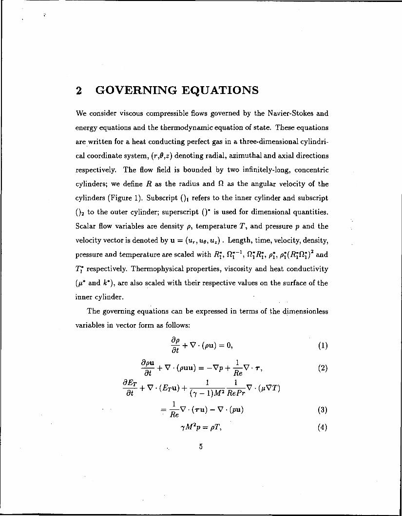
The governing equations can be expressed in terms of the dimensionless

variables in vector form as follows:

, (1)

V.r , (2)

_L V. (ru) - V • (pa) (3)

(4)

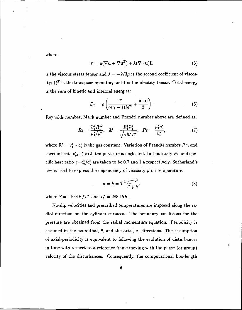
where

r = /i(Vu + VuT) + A(V • u)I. (5)

is the viscous stress tensor and A = — 2/3/z is the second coefficient of viscos-

ity; ()T is the transpose operator, and I is the identity tensor. Total energy

is the sum of kinetic and internal energies:

/ T u - u \ •

Reynolds number, Mach number and Prandtl number above are defined as:

where R* = c* — c* is the gas constant. Variation of Prandtl number Pr, and

specific heats c*, c* with temperature is neglected. In this study Pr and spe-

cific heat ratio 7=c*/c* are taken to be 0.7 and 1.4 respectively. Sutherland's

law is used to express the dependency of viscosity /z on temperature,

, = * = T t i± , (8)

where S = UOAK/Tf and 7\* = 28S.15K.

No-slip velocities and prescribed temperatures are imposed along the ra-

dial direction on the cylinder surfaces. The boundary conditions for the

pressure are obtained from the radial momentum equation. Periodicity is

assumed in the azimuthal, 0, and the axial, z, directions. The assumption

of axial-periodicity is equivalent to following the evolution of disturbances

in time with respect to a reference frame moving with the phase (or group)

velocity of the disturbances. Consequently, the computational box-length

corresponds to the largest wavelength represented in the solution. The choice

of the box-length is not a trivial task as the most critical waves should be

included in the simulation. For this purpose, results from an earlier linear

stability analysis of this problem11 were used to determine the wavelength

of the most critical disturbances.

The base flow is a steady solution of the governing equations. For this

purpose, axisymmetric two-dimensional flow in the (r,0) plane is assumed

so that all variables depend only on the radial coordinate, r. Velocity com-

ponents in the axial direction, z, and the radial direction, r, are taken to

be zero for a purely azimuthal base flow. The resulting system of ordinary

differential equations are then solved as a boundary value problem.11

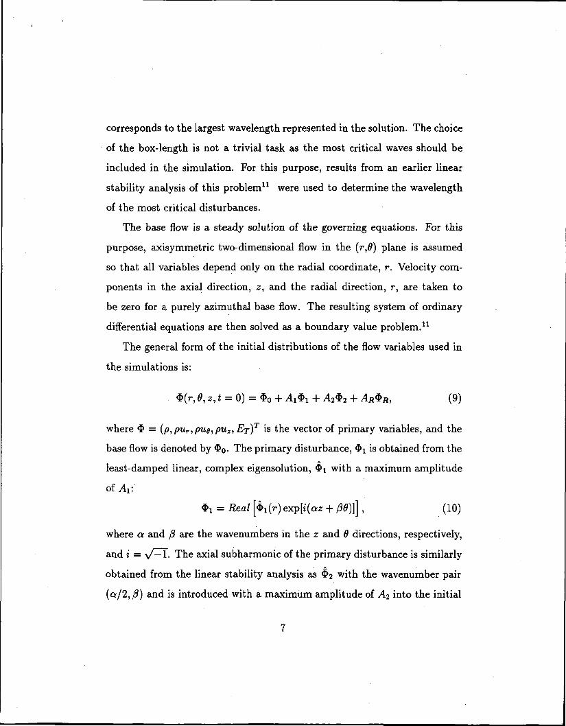
The general form of the initial distributions of the flow variables used in

the simulations is:

$(r,6,z,t = Q) = $0 + Al$l + A3*2 + AR*R, (9)

where $ = (p,pur,puo,puz,ET)T is the vector of primary variables, and the

base flow is denoted by $o- The primary disturbance, $1 is obtained from the

least-damped linear, complex eigensolution, $1 with a maximum amplitude

of AI:

$! = Real [4i(r) exp[i(az + ft9)]] , (10)

where a and ft are the wavenumbers in the z and 0 directions, respectively,

and i = \/— 1. The axial subharmonic of the primary disturbance is similarly

obtained from the linear stability analysis as $2 with the wavenumber pair

(a/2, ft) and is introduced with a maximum amplitude of A2 into the initial

field;

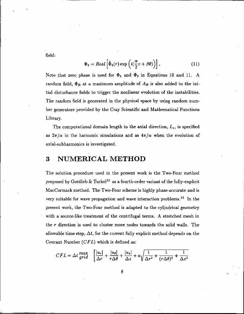
$2 = Real [$2(r)exp (t(|* + /M))] , (11)

Note that zero phase is used for $1 and $2 in Equations 10 and 11. A

random field, $H at a maximum amplitude of AH is also added to the ini-

tial disturbance fields to trigger the nonlinear evolution of the instabilities.

The random field is generated in the physical space by using random num-

ber generators provided by the Cray Scientific and Mathematical Functions

Library.

The computational domain length in the axial direction, Lz, is specified

as 2ir/a in the harmonic simulations and as 4ff/a when the evolution of

axial-subharmonics is investigated.

3 NUMERICAL METHOD

The solution procedure used in the present work is the Two-Four method

proposed by Gottlieb & Turkel12 as a fourth-order variant of the fully-explicit

MacCormack method. The Two-Four scheme is highly phase-accurate and is

very suitable for wave propagation and wave interaction problems.13 In the

present work, the Two-Four method is adapted to the cylindrical geometry

with a source-like treatment of the centrifugal terms. A stretched mesh in

the r direction is used to cluster more nodes towards the solid walls. The

allowable time step, A£, for the current fully explicit method depends on the

Courant Number (CFL) which is defined as:

CFL = A* Kl M |«,| / i , i , i"I 7^7 "I I r o\ ~: o T ~, r~TTT T

Ar rA0 Az V Ar2 (rA0)2 A*2

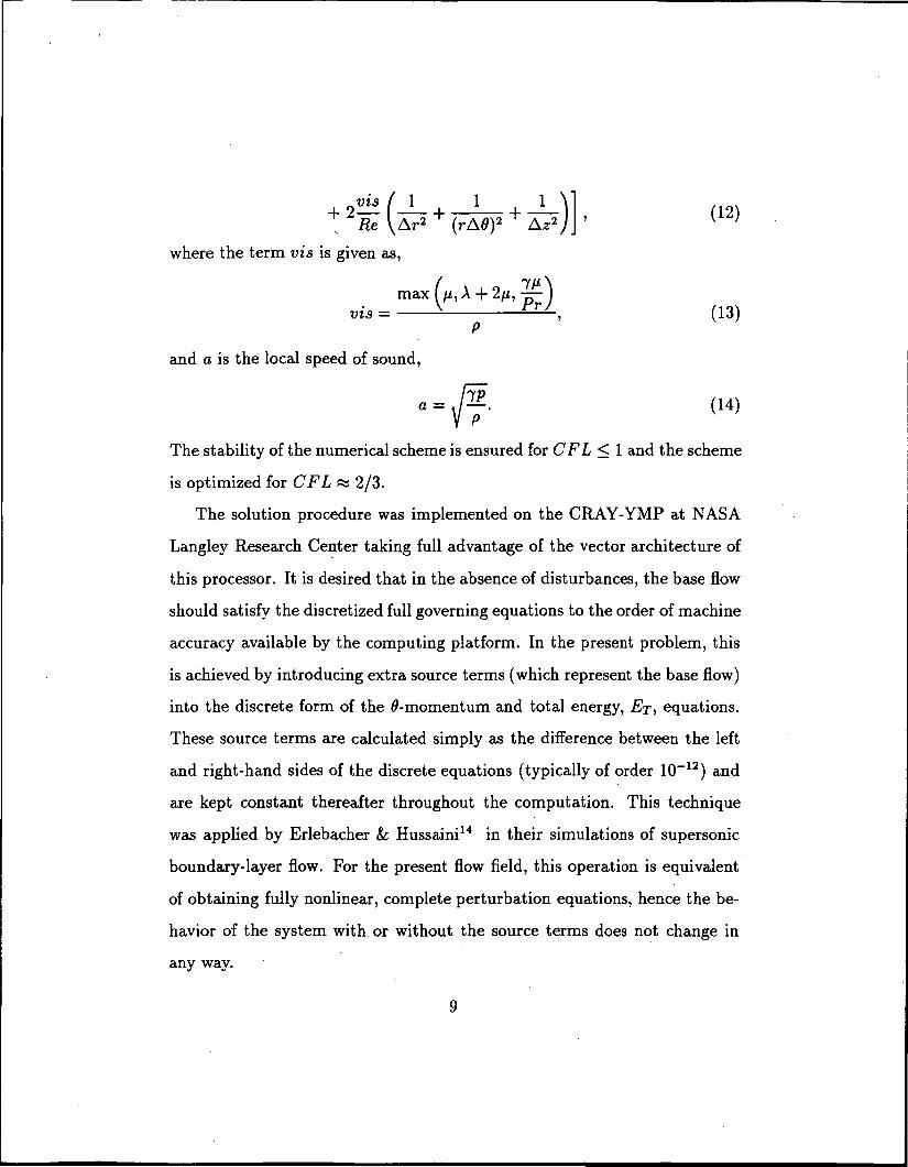
1(rA0)2 Az2/J '

where the term vis is given as,

maxfu A + 2u -**'vis =

P

and a is the local speed of sound,

P

The stability of the numerical scheme is ensured for CFL < 1 and the scheme

is optimized for CFL « 2/3.

The solution procedure was implemented on the CRAY-YMP at NASA

Langley Research Center taking full advantage of the vector architecture of

this processor. It is desired that in the absence of disturbances, the base flow

should satisfy the discretized full governing equations to the order of machine

accuracy available by the computing platform. In the present problem, this

is achieved by introducing extra source terms (which represent the base flow)

into the discrete form of the ^-momentum and total energy, ET, equations.

These source terms are calculated simply as the difference between the left

and right-hand sides of the discrete equations (typically of order 10~12) and

are kept constant thereafter throughout the computation. This technique

was applied by Erlebacher & Hussaini14 in their simulations of supersonic

boundary-layer flow. For the present flow field, this operation is equivalent

of obtaining fully nonlinear, complete perturbation equations, hence the be-

havior of the system with or without the source terms does not change in

any way.

4 RESULTS

4.1 Initial Disturbances

The Navier-Stokes solver described in Section 4 was tested extensively by

comparisons with the linear theory; these results are reported elsewhere.11

Accordingly, the amplitude and phase agreement between the linear theory

and the direct numerical simulation is better than 1.0%.

In the present work, we investigate the nonlinear temporal evolution of

compressible flow in a wide gap (Ri/R? = 0.5) between infinitely-long, con-

centric cylinders with equal and opposite rotation speeds (f^/^i = —!)•

Direct numerical simulations were performed at a supersonic Mach number

of M = 2.0 and at a Reynolds number of Re = 2,000. According to the linear

stability analysis11 the primary instability is a three-dimensional, traveling

wave when the cylinders are in the counter-rotating configuration at finite

Mach numbers. At Re = 2,000 a wide band of linearly unstable distur-

bances exist with different axial and azimuthal wavenumbers (a, /?) and the

combination of a = 19.0 and /? = 1 gives the highest growth rate; due to

the circular geometry, /? can assume only integer values. For these parameter

values, a high-resolution linear analysis with 121 nodes in the radial direction

generates the temporal eigenvalue (complex frequency) u = 0.5168+ zO.9758,

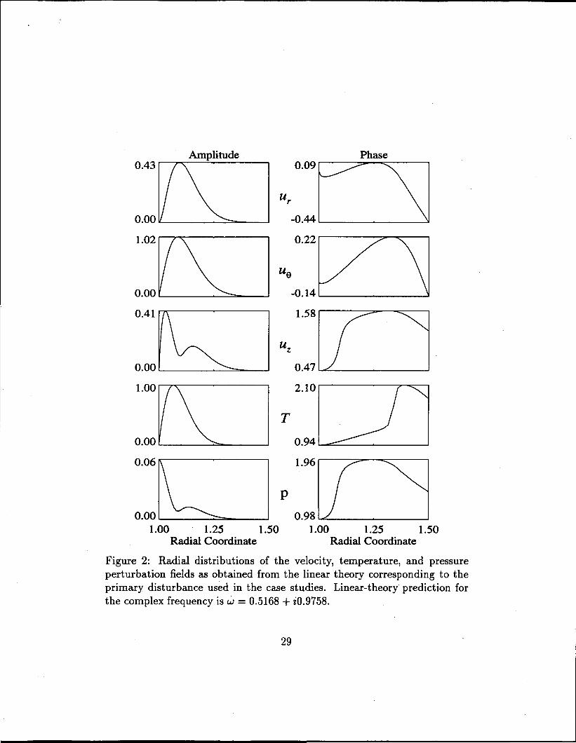
whose imaginary part is the growth rate. The corresponding eigenfunctions

(Figure 2) were used as the primary disturbance field ($1 in Eq. 11) for the

Navier-Stokes simulations and reveal a one-cell structure with maxima closer

to the inner cylinder and quiescent behavior in the outer half of the domain.

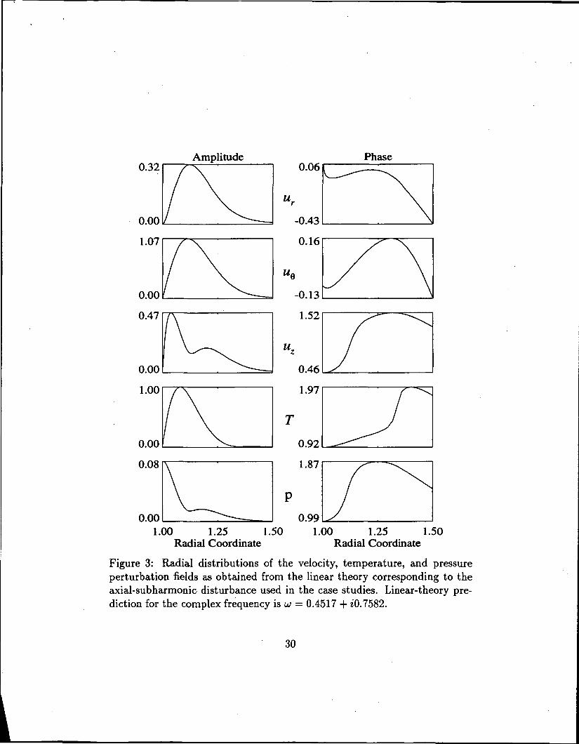
The eigenfunctions for the axial subharmonic ($2 in Eq. 11) were obtained

10

in a similar manner and are presented in Figure 3.

In the subsequent sections, we report the results from three separate di-

rect numerical simulations. The first simulation discloses the evolution of the

harmonics in the absence of the subharmonic generation, whereas the second

allows for the evolution of the subharmonics. The last simulation is initial-

ized with comparable finite amplitudes of the primary and axial-subharmonic

disturbances with zero phase difference, revealing the effects of forced sub-

harmonics. We analyze the nonlinear development of the disturbance field

for each case.

4.2 Harmonic Development

This simulation was initialized with the primary disturbance imposed on the

base flow with a maximum amplitude of A\ = 10~3 together with a random

disturbance field of amplitude Ap, = 10~6. The computational domain was

chosen to accommodate one full axial wavelength of the fundamental distur-

bance (Lz = 27r/a). The temporal evolution of the disturbances was then

studied with a computational grid resolution of 65 x 66 x 34 in the radial,

azimuthal, and axial directions, respectively. During the course of the sim-

ulation, the solution fields were interpolated onto a high-resolution grid of

65 x 66 x 66 and integrated in time at this resolution. The complete agreement

between these two simulations indicate that solutions are grid independent.

In order to analyze the data, we first performed one-dimensional Fourier

expansions in one periodic direction (either 6 or z) and followed the time

evolution of the maximum Fourier amplitudes. For example, an expansion

11

of the field variable (f> in a one-dimensional Fourier series along the axial

direction, z, can be written as:

(j>(r, z, d,t) = ^ <j>(r, ki,Q, t) exp (ikiaz), (15)

where \k i \ < ^Nz and Nz is the number of nodes in the z direction. The

maximum amplitude is found in the (r, 0) plane:

.,, . max / i>x f,^A(ki,t) = fr m (qxp ), (16)

where ()* denotes the complex conjugate. Similarly, a one-dimensional Fourier

expansion in the azimuthal direction , 0, yields:

where |&2| < %Ng and Ng is the number of nodes in the 9 direction. This

time, the maximum amplitude is found in the (r, z) plane:

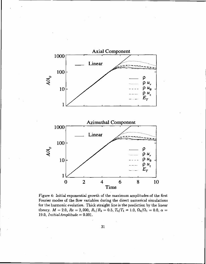
As predicted by the linear theory, the initial growth of the primary dis-

turbance is exponential. In Figure 4, the time evolution of A(k\ = l,t) and

A(kz = 1, t) is compared with the linear theory. The quantitative comparison

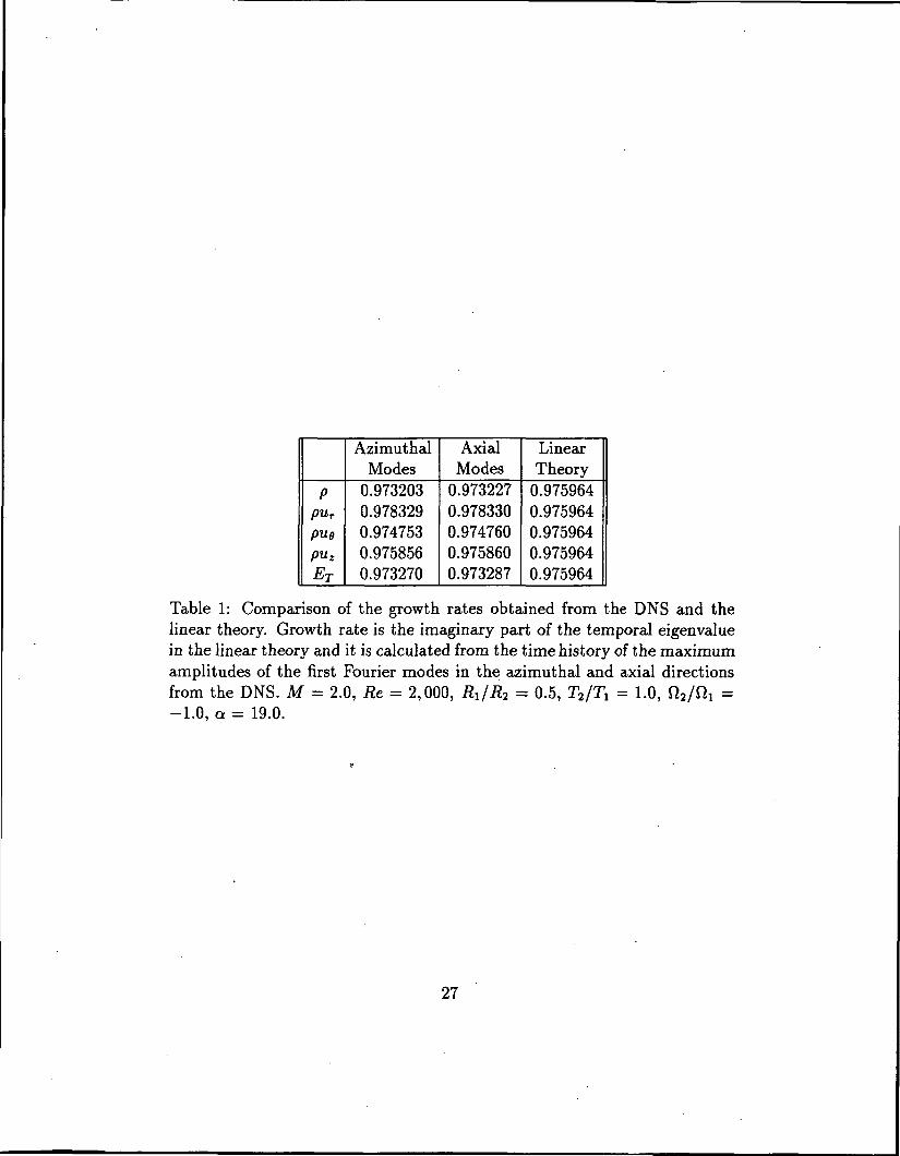
of the growth rates in Table 1 reveals good agreement in the initial stage.

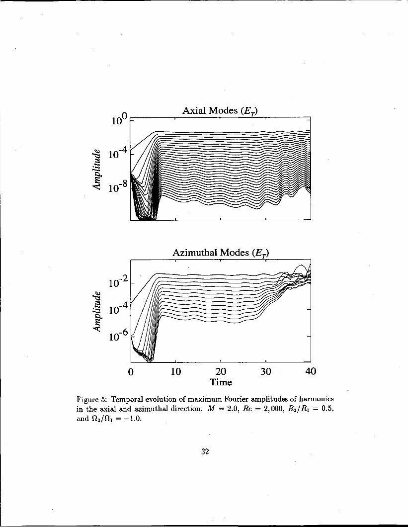
The time history of A(ki,t) and A(k-i,i) is presented in Figure 5 for the

total energy, ET- In each of these plots, the topmost curve represents the

first wavenumber (fci = 1 or &2 = 1 in Eq. (16) ) and the lower curves are

the harmonics in ascending order. The amplitudes of the harmonics first

12

decay and then are energized and follow the rapid growth of the primary

mode. The excitation of the harmonics takes place in a perfect hierarchy in

which the smallest wavenumber becomes energized first, reaches saturation

at a finite amplitude and then transfers its excess energy to the next smaller

wavenumber. This cascading process continues until all the modes reach a

nonlinearly quasi-saturated plateau stage along which the disturbances are

sustained at finite amplitudes. The whole range of harmonics, not a few

wavenumbers, in both the axial and azimuthal directions is supported in this

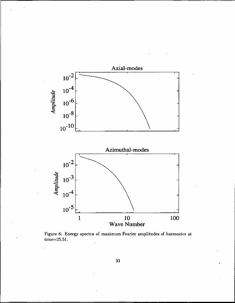
stage. Power spectra of A, the maximum amplitude of the total energy ET

as defined in Eqs. (16) and (17), at t = 25.51 (Figure 6) are smooth and

continous with a fast decay towards the large wavenumbers indicative of the

sufficient grid resolution used in the numerical solution at this stage. The

smoothness of the spectra is related to the continous cascade of energy from

the smaller wavenumbers.

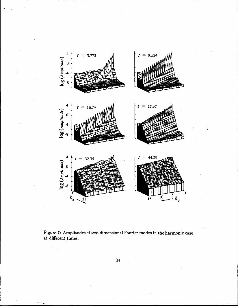
Figure 7 illustrates the generation of the harmonics in the two-dimensional

wavenumber space. Here, ET is expanded in a Fourier series in 0 and z di-

rections as:

where \k i \ < j-/V2, |&2| < \Ng, Nz and Ng are the number of nodes in z and

0 directions, respectively. The amplitude of these modes are defined as:

r. (20)R\

In the present analysis, the quantity given by Eq. (20) refers to the energy

contained in the spectral mode (fci, fcj). This definition of modal energy is not

13

unique and differs from the incompressible definition. However, the present

approach has the advantage of containing both the kinetic and internal en-

ergies of the disturbance fields. Moreover, the analysis based on the present

definition gives a coherent and consistent picture of the events in the physical

space as well as in the spectral space.

As depicted in Figure 5, the harmonics are energized sequentially as time

progresses. Also, new peaks appear in the two-dimensional Fourier spectrum

shown in Figure 7 in a systematic fashion along the axial-harmonics. The

direction of this hierarchial generation of harmonics is initially:

(21)

where n = 1,2, ...^Nz. Once the harmonics are energized in this hierar-

chy, energy is transferred to the other wavenumbers in the two-dimensional

wavenumber space. At later times, a uniform distribution of the amplitudes

is approached with gradual decay towards the smaller wavenumbers. It is

interesting to note that the amplitude-decay is much slower in the azimuthal

direction than in the axial direction. Therefore, the azimuthal mesh resolu-

tion requirements became prohibitive beyond t = 40.0.

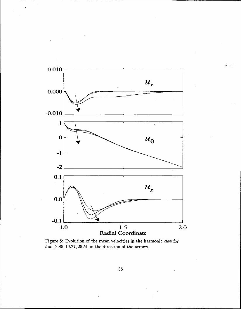
The main energy source in this temporal evolution is the external torque

applied at the rotating cylinders. Figure 8 presents the mean velocities (av-

eraged in the z-9 plane) at selected times. The increase in the gradients close

to the inner cylinder is due to more efficient energy and momentum transfer.

Relatively flat portions of the ug profiles for about r « 1.1 indicate enhanced

momentum-mixing in that region. The development of non-zero ur and uz

is related to the nonlinear distortions of the initially sinusoidal disturbance

14

fields. Consequently, in the inner half of the gap, the mean flow is no longer

purely azimuthal but has a weakly swirling component.

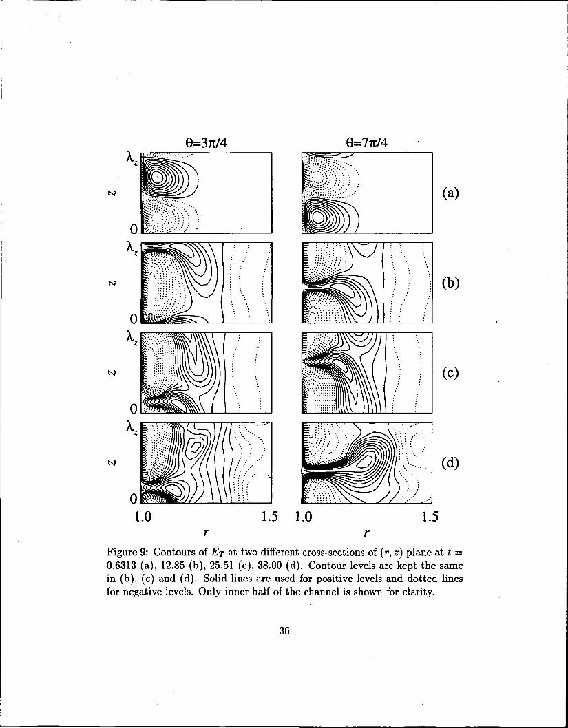
The events in the spectral and physical spaces can be interconnected

through the inspection of instantaneous disturbance fields. Figure 9 presents

contour plots of disturbance total energy, ET, in several (r-z) planes. During

the early stage, t — 0.6313, the initially imposed randomness quickly dies

and the fundamental mode with its characteristic sinusoidal variation dom-

inates the flow field at this cross-section. At later times, as the harmonics

are energized and the plateau stage is reached, the formation of a jet-like

structure is observed close to the inner wall. The harmonics are generated in

phase with each other; consequently, their superposition leads to this high-

shear-layer formation. The jet-like structure expands towards the center of

the gap in the shape of a mushroom but does not quite extend into the

outer half of the gap so that this region remains stable. Along the plateau

stage (t > 20), these jets or mushroom-like ejection structures promote even

higher-shear layers with stronger gradients close to the inner wall. Three-

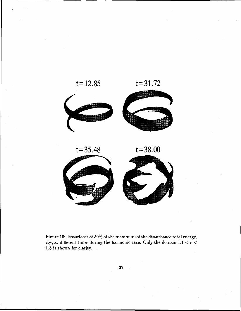
dimensional isosurfaces of disturbance total energy, ET, at the levels of 50%

of the maximum of the disturbance field, are presented in Figure 10 to illus-

trate this sequence of events in greater detail. In the beginning of the plateau

(t = 12.85), the isosurfaces are perfectly spiral, indicating the dominance of

the fundamental mode. The development of high shear layers is discernible in

the high energy isosurface as it narrows close the inner cylinder and spreads

towards the center of the channel. Along the plateau (t = 31.72), the jets

get thinner and the structures become susceptible to the higher instability

15

mechanisms as evident from the waviness superimposed on the spirals. This

critical wavy development in the azimuthal direction is also evident from

the increasing amplitudes and the crowdening if the azimuthal spectrum for

t > 30 in Figure 5. Eventually (t=35.48), the spiral symmetry is lost as the

high energy structure locally detaches from the wall generating small-scale

structures during the breakdown process. The investigation of the physics

of flow transition beyond this stage would require an extremely high spatial

and temporal resolution not affordable by the computer resources available

for this study.

4.3 Subharmonic Development

In this simulation, the computational domain is extended to accommodate

two axial-wavelengths of the fundamental disturbance (L = 1\z = 47T/a) in

order to allow the generation and the evolution of the axial-subharmonics of

the fundamental mode. For this case, the number of nodes is increased to

81 x 130 x 102 in the radial, azimuthal, and axial directions, respectively.

The other parameters and the initial conditions are kept the same as in the

previous harmonic simulation. The first subharmonic mode is excluded from

the initial conditions (A2 = 0) and can be generated only through nonlinear

mechanisms.

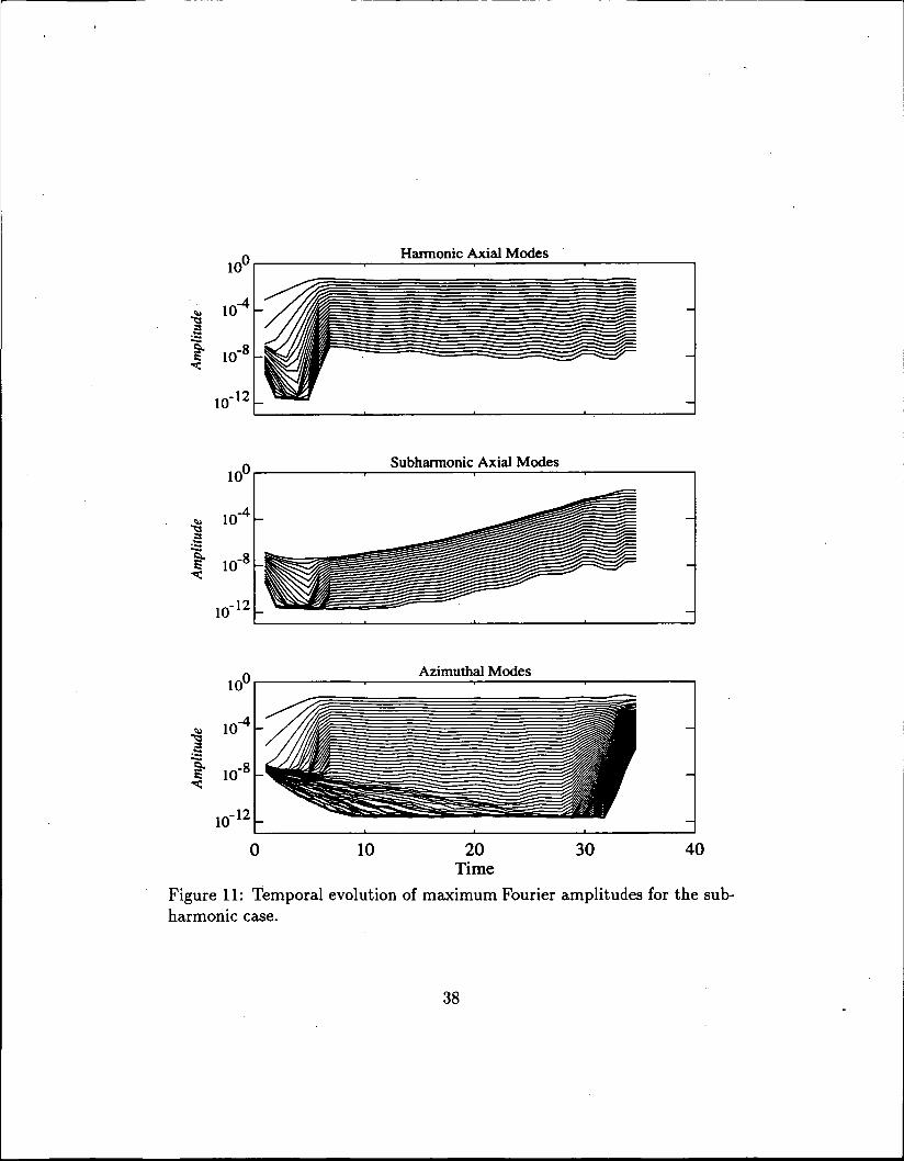
Figure 11 depicts a similar evolution of the amplitudes of the one-dimensional

Fourier components as in the harmonic case: initial rapid growth of the fun-

damental mode saturates to reach a plateau stage. For all the simulations

performed in the present study, the nonlinear saturation is achieved over ap-

16

proximately one rotation of the cylinders (period = 27r/0i = 6.28). There-

fore, the mechanism for the generation and the immediate evolution of both

harmonic or subharmonic disturbances must be the inviscid, rotational insta-

bilities. As the disturbances evolve and attain finite amplitudes, a nonlinear

saturation state is reached.

The evolution of the subharmonics is distinct from that of the harmonics.

Starting from the small-amplitude random initial disturbance field, subhar-

monic modes neither reach the saturation level nor do they catch up with

the harmonics until the very late stages of the transition process.

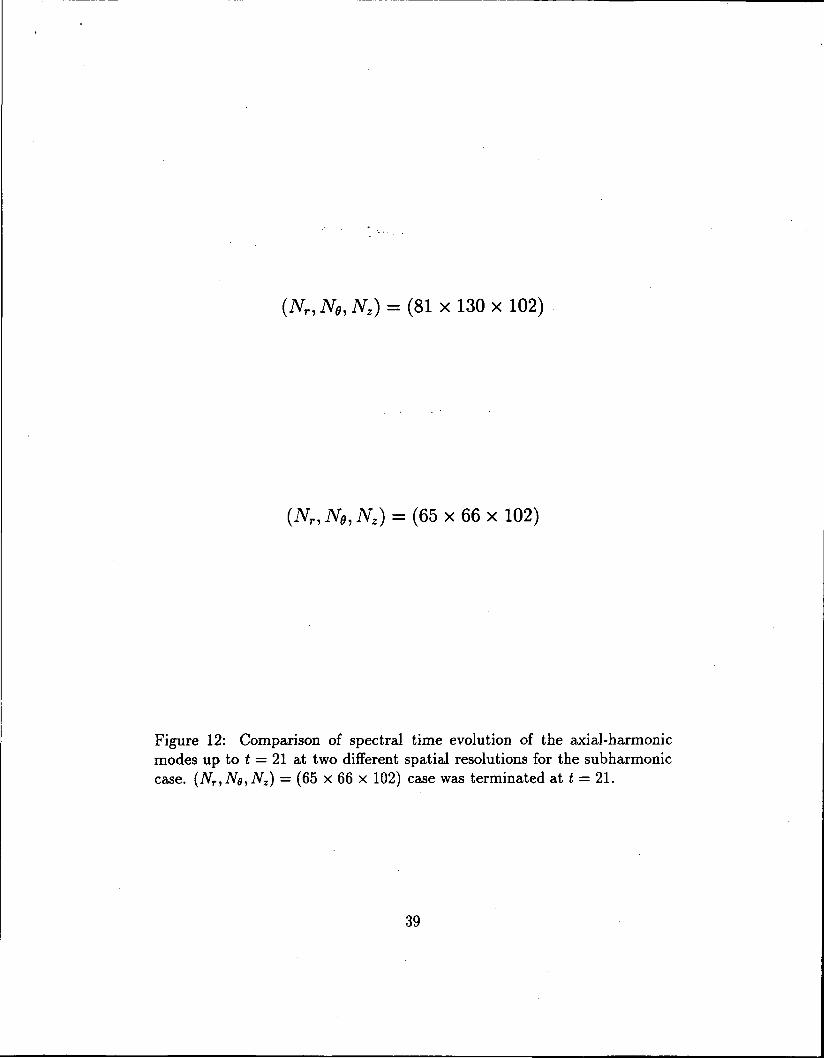
Figure 12 compares the spectral time evolution of the axial-harmonic

modes from a preliminary run performed up to t = 21 at a resolution of

65 x 66 x 102 with the 81 x 66 x 102 high resolution case. This comparison

reveals a similar behavior providing further justification to the adequacy of

the computational grid used throughout the present study.

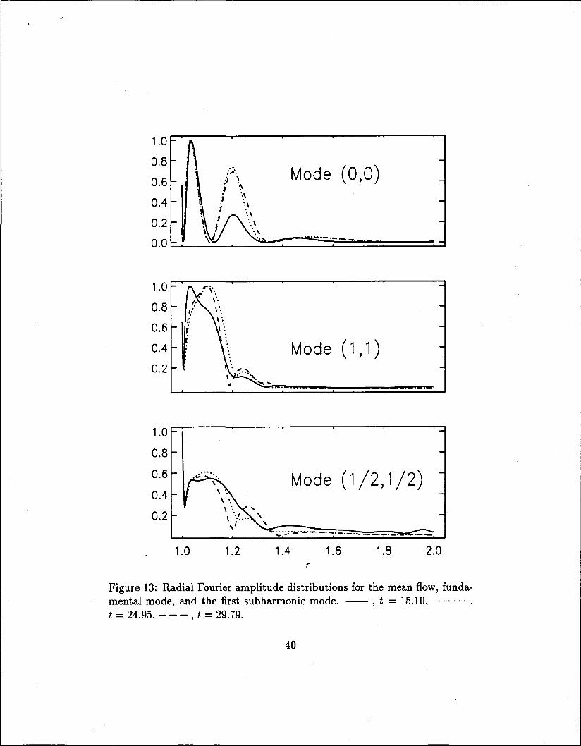
Figure 13 shows the radial distributions of the Fourier amplitudes for

the mean flow, the fundamental mode, and the first subharmonic mode at

different times. Maximum amplitudes occur close to the inner cylinder, and

strong development of a secondary extremum for r « 1.2 is observed at later

times. The amplitudes at the inner cylinder surface are not zero, because as

the kinetic energy of the disturbances diminishes to zero, the internal energy

content actually increases very rapidly in the near-wall region.

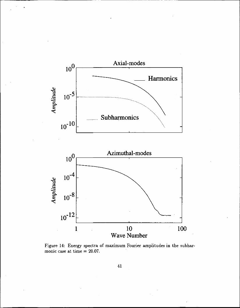
In Figure 14, the subharmonic components attain a well-developed spec-

trum showing the decay of energy towards higher wavenumbers. The spectra

of subharmonics and harmonics are similar but separate, suggesting a dif-

17

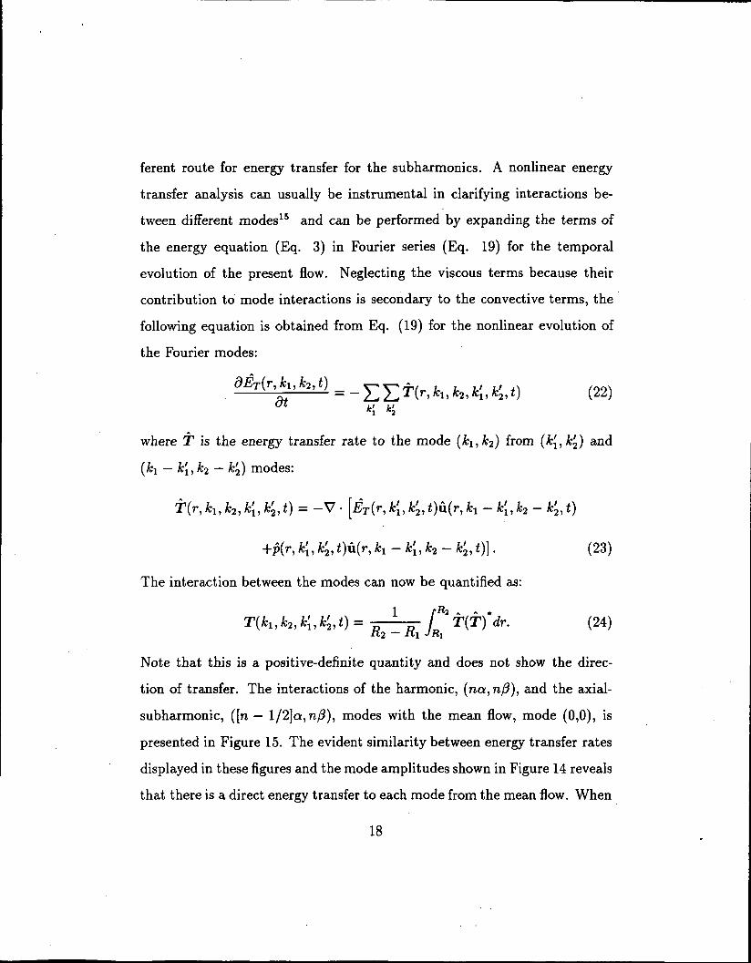
ferent route for energy transfer for the subharmonics. A nonlinear energy

transfer analysis can usually be instrumental in clarifying interactions be-

tween different modes15 and can be performed by expanding the terms of

the energy equation (Eq. 3) in Fourier series (Eq. 19) for the temporal

evolution of the present flow. Neglecting the viscous terms because their

contribution to mode interactions is secondary to the convective terms, the

following equation is obtained from Eq. (19) for the nonlinear evolution of

the Fourier modes:

*!,*,, fcj.^t) (22)

where T is the energy transfer rate to the mode (ki,k2) from (k(,k'2) and

(ki — k{, k-2 — k'2) modes:

+p(r, *!,*£, <)u(r, A* - k[, k2 - fc£, *)] . (23)

The interaction between the modes can now be quantified as:

r. (24)

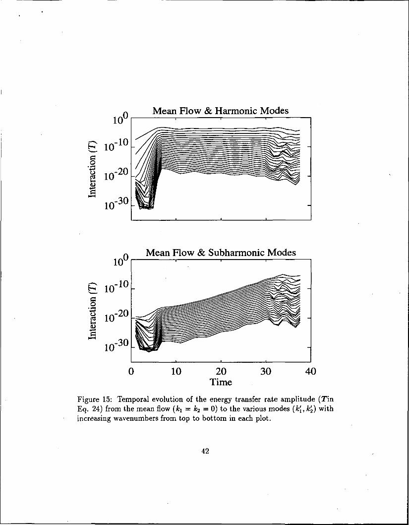
Note that this is a positive-definite quantity and does not show the direc-

tion of transfer. The interactions of the harmonic, (na, n(3), and the axial-

subharmonic, ([n — l/2]a, n^), modes with the mean flow, mode (0,0), is

presented in Figure 15. The evident similarity between energy transfer rates

displayed in these figures and the mode amplitudes shown in Figure 14 reveals

that there is a direct energy transfer to each mode from the mean flow. When

18

a harmonic mode reaches saturation so does its interaction with the mean

flow. Along the saturation state, the mean flow continues to supply energy to

the modes and the modes which reach saturation transfer their excess energy

to the higher modes down the nonlinear energy cascade. In the meantime,

the subharmonic modes never reach saturation and their interaction with the

mean flow continously increases during the simulation.

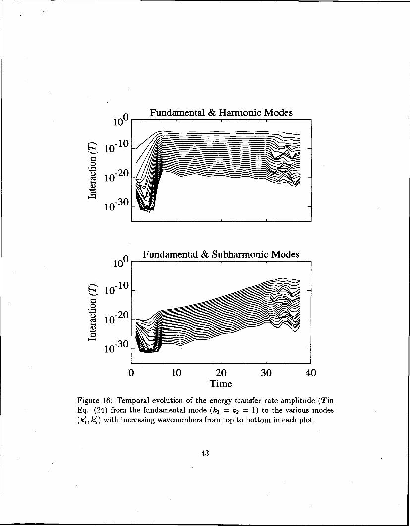
Interactions of the fundamental mode, (a, 0), with the other modes (Fig-

ure 16) indicate a similar energy transfer mechanism for the fundamental

compared with the mean mode. Accordingly, the fundamental mode consti-

tutes the next level in the harmonic cascade after the mean flow in trans-

ferring energy to the harmonic and subharmonic modes and this scenario

repeats itself along the harmonic cascade. Considering all modal energy

transfer combinations, when a mode reaches saturation, net energy transfer

to that mode diminishes to zero as the energy cascade continues to operate

in equilibrium.

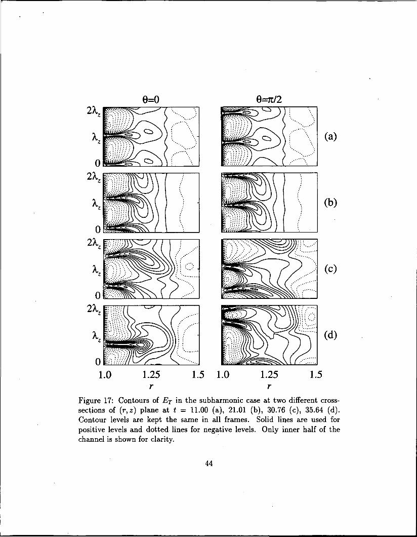
Figure 17 displays the time evolution of the disturbance total energy, ET,

in several (r, z) sections for 0 = 0 and TT. Following the initial exponential-

growth stage, jet-like ejection structures develop as in the harmonic case.

These structures occur with the periodicity of the fundamental disturbance

and are indeed harmonic in nature. At later times, subharmonic structures

develop and compete with the harmonics. The emergence of subharmonic

structures in physical space is the result of merging adjacent ejection struc-

tures yielding a periodicity with twice the wavelength of the fundamental

disturbance in the axial direction. These subharmonic jet-like structures

19

are stronger than their harmonic predecessors and reveal a powerful ejection

extending from the wall region spreading towards the outer cylinder. The

subharmonic structures quickly become susceptible to the higher instabili-

ties leading to flow breakdown and are also accompanied by changes in the

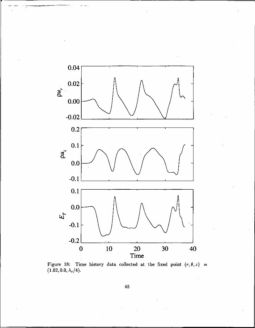
temporal response. In Figure 18, time-history data collected at a fixed point

in space are presented. Quasi-periodic behavior along the plateau stage is

discernible by two sequential peaks followed by two troughs with a period

close to that of the fundamental mode (2ir/Real(u) = 12.16). The distur-

bances have gained appreciable amplitude of about 0.05-0.10 at this stage.

This temporal response is nonlinearly distorted forming spikes concurrent

with the formation of jet-like structures in space. The loss of spatial sym-

metry takes place simultaneously with the loss of quasi-periodicity in time,

indicating the end of the plateau stage.

The near-wall events investigated throughout the present study can also

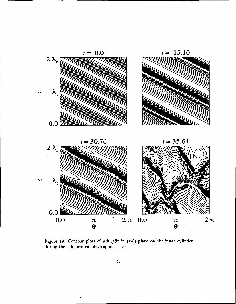
be traced from the the development of equishear lines at the wall. Figure 19

illustrates the development of the disturbance part of pdug/dr at the inner

cylinder wall. Initially, the equishear lines are straight with an inclination of

a//3 in the (z-0) plane tracing the spiral structure imposed by the fundamen-

tal disturbance. Along the plateau stage, the formation of high-shear layers

caused by the strong jet-like structures is indicated from the intensity of the

equishear lines. The flow becomes susceptible to higher instability mecha-

nisms evident from the waviness of these contours at later times and the

breakdown follows the emergence of structures with higher wavenumbers.

20

4.4 Forced Subharmonic Development

The simulation described in Section 4.3 indicated that when subharmonics

are allowed to develop in the computational box by prescribing the appro-

priate box-length, they may dominate over the harmonic structures. In the

previous simulations, although linearly the most unstable mode was chosen

as the primary disturbance, the axial-subharmonics clearly have a crucial

role during the nonlinear stage. To further clarify this issue, in the third

simulation we introduced the subharmonic disturbances in the initial condi-

tions with A-2 = 10~3 together with the harmonic disturbances (A\ = 10~3);

a random field (An = 10~6) was also imposed on the base flow.

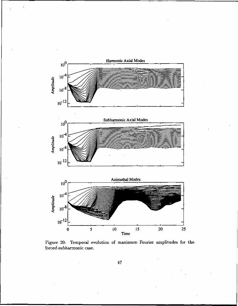
Starting with equal amplitudes for the first subharmonic mode and the

fundamental, during the exponential-growth stage (Figure 20) the axial-

subharmonic modes evolve in a manner similar to the evolution of the har-

monics. Both the subharmonic and the harmonic modes reach finite-amplitude

levels for nonlinear saturation after approximately one rotation of the cylin-

ders. However, the plateau stage is much less well-defined and less stable than

the previous simulations and amplitudes of the azimuthal modes fluctuate

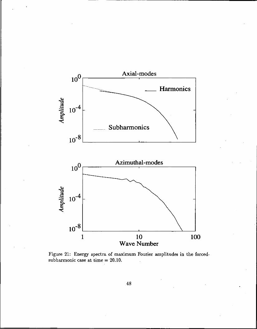
along the plateau. In Figure 21 the amplitude spectra of the one-dimensional

Fourier modes indicate slower decay towards the small wavenumbers com-

pared with the previous simulations and the spectrum of the azimuthal modes

is no longer smooth but contains small-scale oscillations. Consequently, the

forced subharmonics appear to have a detrimental effect on the sustainability

of the plateau stage.

As the amplitudes of the harmonics and subharmonics become compara-

21

ble, nonlinear developments lead directly to the formation of jet-like struc-

tures of the subharmonic type; no initial harmonic stage is observed during

this simulation. Moreover, these structures are no longer confined to the

inner half of the gap but extend further into the outer half which remained

stable during the nonlinear evolution in the previous numerical simulations

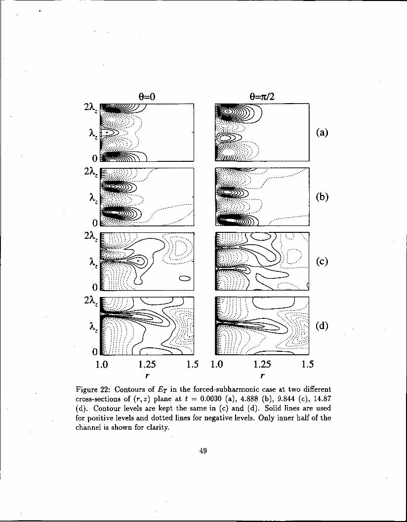
(Sections 4.2 and 4.3). Although the jets do not quite impinge upon the

outer cylinder, they are strong enough to instigate significant activity in the

outer half of the gap (Figure 22).

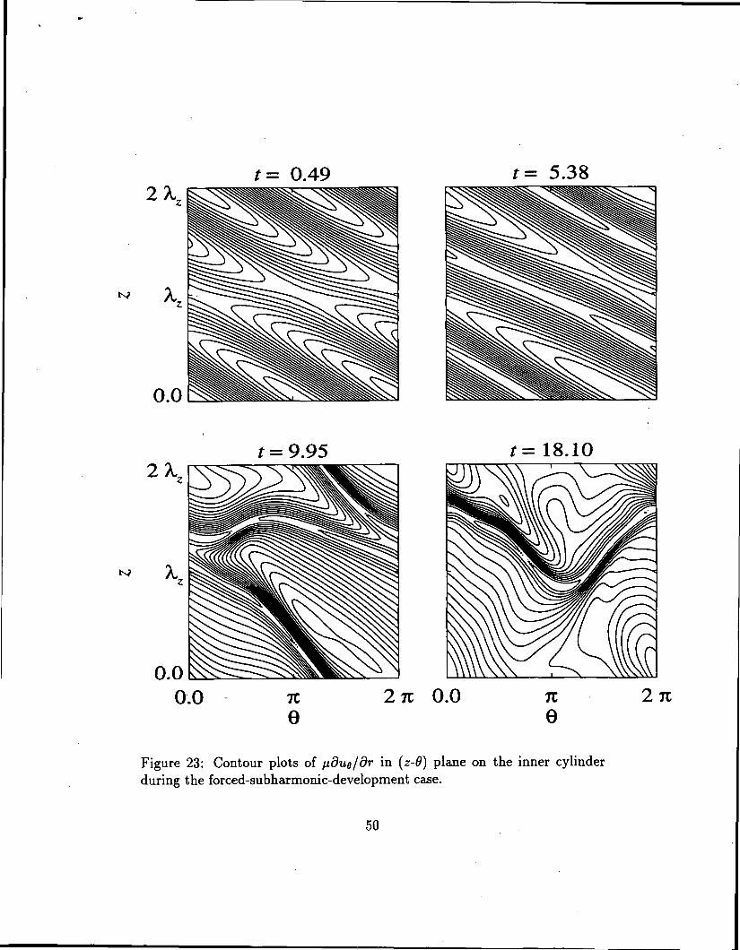
As in the previous case, the formation of high-shear layers is discernible

from the intensification of equishear lines in the contours of the disturbance

part of ndug/dr at the inner cylinder wall (Figure 23). Characteristic of this

simulation is the increasing subharmonic character of the flow field during

the plateau stage. The resulting structures quickly become subject to higher

instability mechanisms and lose their spiral symmetry.

In all of the cases presented in this work, sharp boundary layers form

on both the outer and inner cylinder walls during the nonlinear stage; how-

ever, the ejection type events originate only close to the inner cylinder giving

further indication that they are produced mainly by rotational instability

mechanisms. As the nonlinear evolution progresses, rotational instabilities

interact and compete with viscous instabilities. Instabilities occuring in the

outer region in the forced-subharmonic case is likely to be a product of such

interactions. In all stages of the evolution, compressibility maintains a reces-

sive role and does not cause any peculiar changes in the nature of instabilities

which are nurtured by viscous and centrifugal mechanisms.

22

5 CONCLUSIONS

Three-dimensional direct numerical simulations of the nonlinear evolution

of disturbances in compressible rotating Couette flow were performed at a

moderate Mach number (M = 2.0) and at a Reynolds number of Re =

2000.0. Initial conditions consisted of a random field imposed on the small-

amplitude fundamental and the first axial-subharmonic modes which were

obtained as three-dimensional traveling wave solutions from a high-resolution

linear stability analysis.

The initial growth of the fundamental mode obtained from the present

DNS is in good agreement with the linear stability predictions. The har-

monics and subharmonics first decay in favor of the exponentially-growing

fundamental mode and then become excited and start to grow in the or-

der of increasing wavenumbers. The growth of the modes saturates when

finite amplitudes are reached; this nonlinear saturation state is referred to

as the plateau stage. When excluded from the initial conditions, the axial-

subharmonics do not attain finite amplitudes to reach the plateau stage. For

initial conditions that contain equal amplitude forced subharmonic and the

fundamental disturbances, the subharmonics reach a nonlinearly saturated

state; however, this plateau stage cannot be sustained. Our results suggest

that the axial subharmonic development is the path of transition dominating

the nonlinear evolution of this flow.

Along the plateau stage jet-like structures form carrying the fluid from the

inner cylinder to the center of the gap. In the absence of forced subharmonics,

these ejection events are harmonic structures and tend to merge to attain a

23

subharmonic character as they evolve. Otherwise, for forced subharmonics,

subharmonic jets dominate both the inital and later stages of the transition

process. The jets grow stronger and narrower and become susceptible to

higher instability mechanisms. Eventually, spiral symmetries are broken by

the detachment of the jets from the wall in a non-uniform manner generating

small-scale structures during the process. The end of the plateau stage is also

marked by the loss of quasi-periodicity in the temporal response.

The events during the transition process of this supersonic shear flow are

mainly generated by the interaction of the centrifugal and viscous mecha-

nisms which are prevalent in incompressible shear flows as well. Only in-

directly does compressibility affect the essentially incompressible transition

phenomena in this shear-driven flow.

References

1 G. I. Taylor, "Stability of a viscous fluid contained between two rotating

cylinders", Phil. Trans. A 223, 289 (1923).

2 D. Coles, "Transition in circular Couette flow", J. Fluid Mech. 21,

385 (1965).

3 S. T. Stuart, "On the nonlinear mechanics of wave disturbances in stable

and unstable parallel flows, part 1. the basic behavior in plane poiseuille

flow", J. Fluid Mech. 9, 353 (1960).

4 A. Davey, "The growth of Taylor vortices in flow between rotating cylin-

ders",- J. Fluid Mech. 14, 336 (1962).

24

5 S. T. Stuart, "On the non-linear mechanics of hydrodynamic stability",

J. Fluid Mech. 4, 1 (1958).

6 H. A. Snyder and R. B. Lambert, "Harmonic generation in Taylor vortices

between rotating cylinders", J. Fluid Mech. 26, 545 (1966).

7 A. Lorenzen, G. Pfister, and T. Mullin, "End effects on the transition

to time-dependent motion in the Taylor experiment", Phys. Fluids 26,

10 (1982).

8 C. A. Jones, "On flow between counter-rotating cylinders", J. Fluid Mech.

112, 443 (1982).

9 C. A. Jones, "The transition to wavy Taylor vortices", J. Fluid Mech.

157, 135 (1985).

10 L. M. Mack. "Boundary-layer linear stability theory", Special Course on

Stability and Transition of Laminar Flow, edited by R. Michel (AGARD,

Neuilly sur Seine, France, 1984), AGARD Report No. 709, p. 3-1.

11 F. F. Hatay, S. Biringen, G. Erlebacher, and W. E. Zorumski, "Stability

of high speed compressible, rotating Couette flow", Phys. Fluids A, 5,

393 (1993).

12 D. Gottlieb and E. Turkel, "Dissipative two-four methods for time-

dependent problems", Math. Comput. 30, 703 (1976).

13 S. Biringen and A. Saati, "Comparison of several finite-difference meth-

ods", J. Aircraft 72, 90 (1990).

25

14 G. Erlebacher and M. Y. Hussaini, "Numerical experiments in supersonic

boundary layer stability", Phys. Fluids A 2, 99 (1989).

15 E. M. Saiki, S. Biringen, G. Danabasoglu, and C. L. Streett, "Spatial

simulation of secondary instability in plane channel flow: comparison of

k- and h-type disturbances", J. Fluid Mech. 253, 485 (1993).

26

ppUT

pu&PUZ

EX

AzimuthalModes

0.9732030.9783290.9747530.9758560.973270

AxialModes

0.9732270.9783300.9747600.9758600.973287

LinearTheory

0.9759640.9759640.9759640.9759640.975964

Table 1: Comparison of the growth rates obtained from the DNS and thelinear theory. Growth rate is the imaginary part of the temporal eigenvaluein the linear theory and it is calculated from the time history of the maximumamplitudes of the first Fourier modes in the azimuthal and axial directionsfrom the DNS. M = 2.0, Re = 2,000, R^Ri = 0.5, Tt/Ti = 1.0, fta/J^ =-1.0, a = 19.0.

27

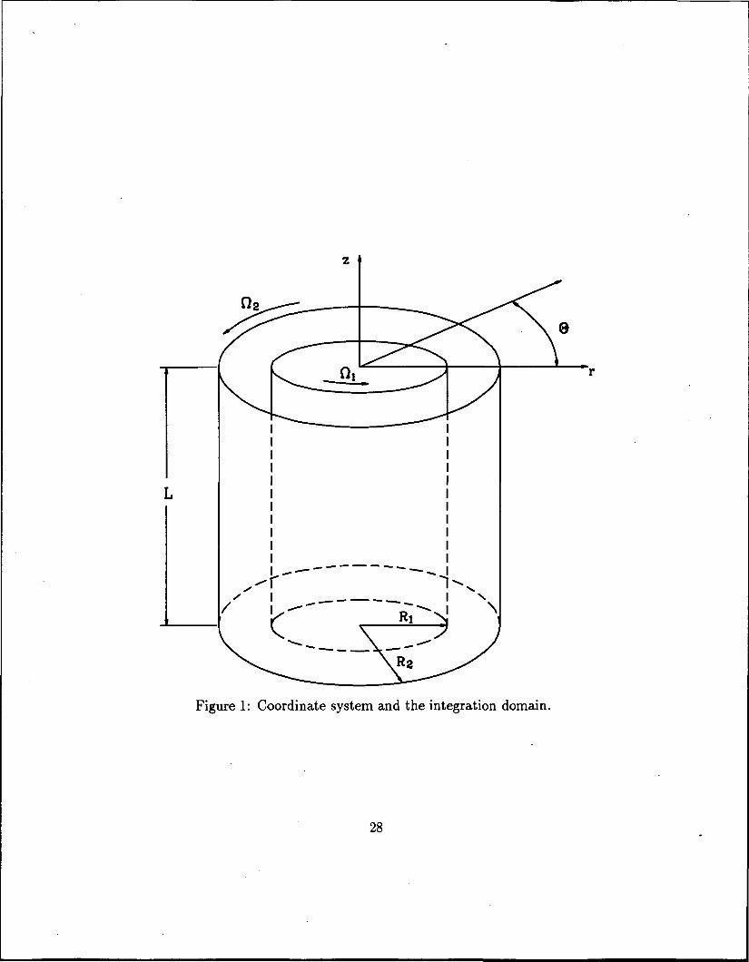
Figure 1: Coordinate system and the integration domain.

28

0.43Amplitude

0.00

0.09Phase

1.00 1.25 1.50Radial Coordinate

1.00 1.25 1.50Radial Coordinate

Figure 2: Radial distributions of the velocity, temperature, and pressureperturbation fields as obtained from the linear theory corresponding to theprimary disturbance used in the case studies. Linear-theory prediction forthe complex frequency is u = 0.5168 + z'0.9758.

29

0.32Amplitude

0.00

0.06Phase

1.00 1.25 1.50Radial Coordinate

1.00 1.25 1.50Radial Coordinate

Figure 3: Radial distributions of the velocity, temperature, and pressureperturbation fields as obtained from the linear theory corresponding to theaxial-subharmonic disturbance used in the case studies. Linear-theory pre-diction for the complex frequency is w = 0.4517 + zO.7582.

30

1000

100-

Axial Component

Azimuthal Component

0

Figure 4: Initial exponential growth of the maximum amplitudes of the firstFourier modes of the flow variables during the direct numerical simulationsfor the harmonic evolution. Thick straight line is the prediction by the lineartheory. M = 2.0, Re = 2,000, Ri/R2 = 0.5, T2/r1 = 1.0, fta/fti = 0.0, a =19.0, Initial Amplitude = 0.001.

31

Axial Modes (£"r)

io-2

0

Azimuthal Modes (ET)

10 20Time

30 40

Figure 5: Temporal evolution oi maximum Fourier amplitudes of harmonicsin the axial and azimuthal direction. M = 2.0, Re = 2,000, R^f'R\ = 0.5,and n2/^i = -1.0.

32

10

10

10

-2

-4

10

10~8

-10

Axial-modes

10-2

.a 10-3

10-4

10-5

Azimuthal-modes

10Wave Number

100

Figure 6: Energy spectra of maximum Fourier amplitudes of harmonics attime=25.51.

33

4

0

15.5 -4

t = 9.534

4

I 0•*•

I-4

t = 16.74 ' t = 27.37

Figure 7: Amplitudes of two-dimensional Fourier modes in the harmonic caseat different times.

34

0.010

0.000

0.1

0.0

-0.11.0

u

1.5Radial Coordinate

2.0

Figure 8: Evolution of the mean velocities in the harmonic case fort = 12.85,19.27,25.51 in the direction of the arrows.

35

0

0

0

6=37t/4

(a)

I

(b)

(c)

(d)

1.0 1.5 1.0 1.5

Figure 9: Contours of ET at two different cross-sections of (r, z) plane at t =0.6313 (a), 12.85 (b), 25.51 (c), 38.00 (d). Contour levels are kept the samein (b), (c) and (d). Solid lines are used for positive levels and dotted linesfor negative levels. Only inner half of the channel is shown for clarity.

36

t= 12.85 t=31.72

t=35.48 t=38.00

Figure 10: Isosurfaces of 50% of the maximum of the disturbance total energy,ET, at different times during the harmonic case. Only the domain 1.1 < r <1.5 is shown for clarity.

37

10

10"

°

ID'8

10,-12

Harmonic Axial Modes

0°

3-4

,-8

Subharmonic Axial Modes

10

10-12

10°

,-410

10,-8

10,-12

0

Azimuthal Modes

10 20Time

30 40

Figure 11: Temporal evolution of maximum Fourier amplitudes for the sub-harmonic case.

38

(Nr, No, Nz) = (81 x 130 x 102)

(Nr, N9, Nz) = (65 x 66 x 102)

Figure 12: Comparison of spectral time evolution of the axial-harmonicmodes up to t = 21 at two different spatial resolutions for the subharmoniccase. (Nr,Ng,Nz) = (65 x 66 x 102) case was terminated at t = 21.

39

1.0

0.8

0.6

0.4

0.2

0.0

Mode (0,0)

1.0

0.8

0.6

0.4

0.2

Mode (1,1)

1.0

0.8

0.6

0.4

0.2

Mode (1/2,1/2)

1.0 1.2 1.4 1.6r

1.8 2.0

Figure 13: Radial Fourier amplitude distributions for the mean flow, funda-mental mode, and the first subharmonic mode. , t = 15.10, ,t = 24.95, , t = 29.79.

40

10'0

.3 10•-»»

I

<'5

10-10

Axial-modes

Harmonics

Subharmonics

-8

10°

-410'•i*

CX O

I 10'8

10-12

Azimuthal-modes

10Wave Number

100

Figure 14: Energy spectra of maximum Fourier amplitudes in the subhar-monic case at time = 20.07.

41

100

io-10

10-30

Mean Flow & Harmonic Modes

Ia

10,0

10-10

10-30

0

Mean Row & Subharmonic Modes

10 20Time

30 40

Figure 15: Temporal evolution of the energy transfer rate amplitude (TinEq. 24) from the mean flow (k\ = &2 = 0) to the various modes (k{, k'2) withincreasing wavenumbers from top to bottom in each plot.

42

100

b 10c

I 10

-10

-20

10-30

Fundamental & Harmonic Modes

010'

e io-10

§1 io-20

10-30

0

Fundamental & Subharmonic Modes

10 20Time

30 40

Figure 16: Temporal evolution of the energy transfer rate amplitude (TinEq. (24) from the fundamental mode (ki = fc2 = 1) to the various modes(&}, fc^) with increasing wavenumbers from top to bottom in each plot.

43

6=0

(a)

(b)

(c)

(d)

1.0 1.25r

1.5

Figure 17: Contours of ET in the subharmonic case at two different cross-sections of (r,z) plane at t = 11.00 (a), 21.01 (b), 30.76 (c), 35.64 (d).Contour levels are kept the same in all frames. Solid lines are used forpositive levels and dotted lines for negative levels. Only inner half of thechannel is shown for clarity.

44

3Q.

3a.

0.04

0.02

0.00

-0.02

0.2

0.1

0.0

-0.1

0.1

0.0

-0.1

-0.20 10 20

Time40

Figure 18: Time history data collected at the fixed point (r, 8, z)(1.02,0.0, A./4).

45

= 0.0 t= 15.10

0.0

Hi

2A,= 30.76 = 35.64

271 0.0 ne

271

Figure 19: Contour plots of (tdug/dr in (z-0) plane on the inner cylinderduring the subharmonic-development case.

46

10°

i«-4

Harmonic Axial Modes

10,-8

10,-12

io-8

10,-12

Subharmonic Axial Modes

10V

ID'8

10,-12

0

Azimuthal Modes

10 15Time

20 25

Figure 20: Temporal evolution of maximum Fourier amplitudes for theforced-subharmonic case.

47

10V

»--4

10-8

Axial-modes

Harmonics

Subharmonics

10,0

10-4

10-8

Azimuthal-modes

10Wave Number

100

Figure 21: Energy spectra of maximum Fourier amplitudes in the forced-subharmonic case at time = 20.10.

48

2A,.0=0

o

2A,

0

(a)

(b)

(c)

(d)

1.0 1.25r

1.5

Figure 22: Contours of ET in the forced-subharmonic case at two differentcross-sections of (r,z) plane at t = 0.0030 (a), 4.888 (b), 9.844 (c), 14.87(d). Contour levels are kept the same in (c) and (d). Solid lines are usedfor positive levels and dotted lines for negative levels. Only inner half of thechannel is shown for clarity.

49

t= 0.49 r= 5.38

0.0

= 9.95 t= 18.10

27T 0.0 n9

27C

Figure 23: Contour plots of ^dug/dr in (z-0) plane on the inner cylinderduring the forced-subharmonic-development case.

50