Numerical Derivatives in Scilab - forge.scilab.org · Numerical Derivatives in Scilab Micha el...

Numerical Derivatives in Scilab

Michael Baudin

May 2009

Abstract

This document present the use of numerical derivatives in Scilab. In thefirst part, we present a result which is surprising when we are not familiar withfloating point numbers. In the second part, we analyse the method to use theoptimal step to compute derivatives with finite differences on floating pointsystems. We present several formulas and their associated optimal steps.In the third part, we present the derivative function, its features and itsperformances.

Contents

1 Introduction 41.1 Introduction . . . . . . . . . . . . . . . . . . . . . . . . . . . . . . . . 41.2 Overview . . . . . . . . . . . . . . . . . . . . . . . . . . . . . . . . . 4

2 A surprising result 42.1 Theory . . . . . . . . . . . . . . . . . . . . . . . . . . . . . . . . . . . 4

2.1.1 Taylor’s formula for univariate functions . . . . . . . . . . . . 52.1.2 Finite differences . . . . . . . . . . . . . . . . . . . . . . . . . 5

2.2 Experiments . . . . . . . . . . . . . . . . . . . . . . . . . . . . . . . . 6

3 Analysis 83.1 Errors in function evaluations . . . . . . . . . . . . . . . . . . . . . . 83.2 Various results for sin(264) . . . . . . . . . . . . . . . . . . . . . . . . 93.3 Floating point implementation of the forward formula . . . . . . . . . 103.4 Numerical experiments with the robust forward formula . . . . . . . . 153.5 Backward formula . . . . . . . . . . . . . . . . . . . . . . . . . . . . . 163.6 Centered formula with 2 points . . . . . . . . . . . . . . . . . . . . . 163.7 Centered formula with 4 points . . . . . . . . . . . . . . . . . . . . . 193.8 Some finite difference formulas for the first derivative . . . . . . . . . 213.9 A three points formula for the second derivative . . . . . . . . . . . . 223.10 Accuracy of finite difference formulas . . . . . . . . . . . . . . . . . . 243.11 A collection of finite difference formulas . . . . . . . . . . . . . . . . . 26

1

4 Finite differences of multivariate functions 284.1 Multivariate functions . . . . . . . . . . . . . . . . . . . . . . . . . . 284.2 Numerical derivatives of multivariate functions . . . . . . . . . . . . . 304.3 Derivatives of a multivariate function in Scilab . . . . . . . . . . . . . 314.4 Derivatives of a vectorial function with Scilab . . . . . . . . . . . . . 334.5 Computing higher degree derivatives . . . . . . . . . . . . . . . . . . 354.6 Nested derivatives with Scilab . . . . . . . . . . . . . . . . . . . . . . 374.7 Computing derivatives with more accuracy . . . . . . . . . . . . . . . 394.8 Taking into account bounds on parameters . . . . . . . . . . . . . . . 41

5 The derivative function 415.1 Overview . . . . . . . . . . . . . . . . . . . . . . . . . . . . . . . . . 415.2 Varying order to check accuracy . . . . . . . . . . . . . . . . . . . . . 425.3 Orthogonal matrix . . . . . . . . . . . . . . . . . . . . . . . . . . . . 425.4 Performance of finite differences . . . . . . . . . . . . . . . . . . . . . 44

6 One more step 47

7 Automatically computing the coefficients 497.1 The coefficients of finite difference formulas . . . . . . . . . . . . . . . 497.2 Automatically computings the coefficients . . . . . . . . . . . . . . . 517.3 Computings the coefficients in Scilab . . . . . . . . . . . . . . . . . . 52

8 Notes and references 54

9 Exercises 55

10 Acknowledgments 57

Bibliography 57

Index 58

2

Copyright c© 2008-2009 - Michael BaudinThis file must be used under the terms of the Creative Commons Attribution-

ShareAlike 3.0 Unported License:

http://creativecommons.org/licenses/by-sa/3.0

3


1 Introduction

1.1 Introduction

This document is an open-source project. The LATEX sources are available on theScilab Forge:

http://forge.scilab.org/index.php/p/docnumder/

The LATEX sources are provided under the terms of the Creative Commons Attribu-tion ShareAlike 3.0 Unported License:


The Scilab scripts are provided on the Forge, inside the project, under the scripts

sub-directory. The scripts are available under the CeCiLL licence:

http://www.cecill.info/licences/Licence_CeCILL_V2-en.txt

1.2 Overview

In this document, we analyse the computation of the numerical derivative of a givenfunction. Before getting into the details, we briefly motivate the need for approxi-mate numerical derivatives.

Consider the situation where we want to solve an optimization problem with amethod which requires the gradient of the cost function. In simple cases, we canprovide the exact gradient. The practical computation may be performed ”by hand”with paper and pencil. If the function is more complicated, we can perform thecomputation with a symbolic computing system (such as Maple or Mathematica).If some situations, this is not possible. In most practical situations, indeed, the for-mula involved in the computation is extremely complicated. In this case, numericalderivatives can provide an accurate evaluation of the gradient. Other methods tocompute the gradient are base on adjoint equations and on automatic differentia-tion. In this document, we focus on numerical derivatives methods because Scilabprovide commands for this purpose.

2 A surprising result

In this section, we present surprising results which occur when we consider a functionof one variable only. We derive the forward numerical derivative based on the Taylorexpansion of a function with one variable. Then we present a numerical experimentbased on this formula, with decreasing step sizes.

This section was first published in [3].

2.1 Theory

Finite differences methods approximate the derivative of a given function f based onfunction values only. In this section, we present the forward derivative, which allows

4

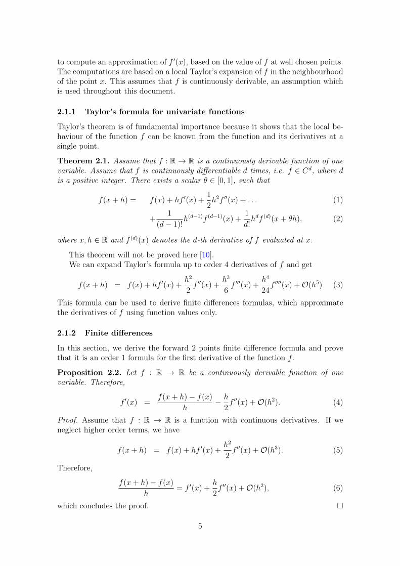
http://forge.scilab.org/index.php/p/docnumder/


http://www.cecill.info/licences/Licence_CeCILL_V2-en.txt

to compute an approximation of f ′(x), based on the value of f at well chosen points.The computations are based on a local Taylor’s expansion of f in the neighbourhoodof the point x. This assumes that f is continuously derivable, an assumption whichis used throughout this document.

2.1.1 Taylor’s formula for univariate functions

Taylor’s theorem is of fundamental importance because it shows that the local be-haviour of the function f can be known from the function and its derivatives at asingle point.

Theorem 2.1. Assume that f : R→ R is a continuously derivable function of onevariable. Assume that f is continuously differentiable d times, i.e. f ∈ Cd, where dis a positive integer. There exists a scalar θ ∈ [0, 1], such that

f(x+ h) = f(x) + hf ′(x) +1

2h2f ′′(x) + . . . (1)

+1

(d− 1)!h(d−1)f (d−1)(x) +

1

d!hdf (d)(x+ θh), (2)

where x, h ∈ R and f (d)(x) denotes the d-th derivative of f evaluated at x.

This theorem will not be proved here [10].We can expand Taylor’s formula up to order 4 derivatives of f and get

f(x+ h) = f(x) + hf ′(x) +h2

2f ′′(x) +

h3

6f ′′′(x) +

h4

24f ′′′′(x) +O(h5) (3)

This formula can be used to derive finite differences formulas, which approximatethe derivatives of f using function values only.

2.1.2 Finite differences

In this section, we derive the forward 2 points finite difference formula and provethat it is an order 1 formula for the first derivative of the function f .

Proposition 2.2. Let f : R → R be a continuously derivable function of onevariable. Therefore,

f ′(x) =f(x+ h)− f(x)

h− h

2f ′′(x) +O(h2). (4)

Proof. Assume that f : R → R is a function with continuous derivatives. If weneglect higher order terms, we have

f(x+ h) = f(x) + hf ′(x) +h2

2f ′′(x) +O(h3). (5)

Therefore,

f(x+ h)− f(x)

h= f ′(x) +

h

2f ′′(x) +O(h2), (6)

which concludes the proof.

5

Definition 2.3. ( Forward finite difference for f ′) The finite difference formula

Df(x) =f(x+ h)− f(x)

h(7)

is the forward 2 points finite difference for f ′.

The following definition defines the order of a finite difference formula, whichmeasures the accuracy of the formula.

Definition 2.4. ( Order) A finite difference formula Df is of order p > 0 for f (d)

if

Df(x) = f (d)(x) +O(hp). (8)

The equation 4 indicates that the forward 2 points finite difference is an order 1formula for f ′.

Definition 2.5. ( Truncation error) The truncation error of a finite difference for-mula for f (d)(x) is

Et(h) =∣∣Df(x)− f (d)(x)

∣∣ (9)

The equation 4 indicates that the truncation error of the 2 points forward formulais:

Et(h) =h

2|f ′′(x)|, (10)

The truncation error of the equation 10 depends on step h so that decreas-ing the step reduces the truncation error. The previous discussion implies that a(naive) algorithm to compute the numerical derivative of a function of one variableis

f ′(x)← (f(x+ h)− f(x))/h

As we are going to see, the previous algorithm is much more naive that it appears,as it may lead to very inaccurate numerical results.

2.2 Experiments

In this section, we present numerical experiments based on a naive implementationof the forward finite difference formula. We show that a wrong step size h may leadto very inacurate results.

The following Scilab function is a straightforward implementation of the forwardfinite difference formula.

function fp = myfprime(f,x,h)

fp = (f(x+h) - f(x))/h;

endfunction

In the following numerical experiments, we consider the square function f(x) =x2, which derivative is f ′(x) = 2x. The following Scilab script implements the squarefunction.

6

function y = myfunction (x)

y = x*x;

endfunction

The naive idea is that the computed relative error is small when the step h issmall. Because small is not a priori clear, we take εM ≈ 10−16 in double precisionas a good candidate for small.

In order to compare our results, we use the derivative function provided byScilab. The most simple calling sequence of this function is

J = derivative ( F , x )

where F is a given function, x is the point where to compute the derivative and J

is the Jacobian, i.e. the first derivative when the variable x is a simple scalar. Thederivative function provides several methods to compute the derivative. In orderto compare our method with the method used by derivative, we must specify theorder of the method. The calling sequence is then

J = derivative ( F , x , order = o )

where o can be equal to 1, 2 or 4. Our forward formula corresponds to order 1.In the following script, we compare the computed relative error produced by our

naive method with step h = εM and the derivative function with default step andthe order 1 method.

x = 1.0;

fpref = derivative(myfunction ,x);

fpexact = 2.;

e = abs(fpref -fpexact )/ fpexact;

mprintf("Scilab f’’=%e, error=%e\n", fpref ,e);

h = 1.e-16;

fp = myfprime(myfunction ,x,h);

e = abs(fp-fpexact )/ fpexact;

mprintf("Naive f’’=%e, error=%e\n", fp,e);

When executed, the previous script prints out :

Scilab f ’=2.000000e+000, error =7.450581e-009

Naive f ’=0.000000e+000, error =1.000000e+000

Our naive method seems to be quite inaccurate and has not even 1 significantdigit ! The Scilab primitive, instead, has approximately 9 significant digits.

Since our faith is based on the truth of the mathematical theory, which leads toaccurate results in many situations, we choose to perform additional experiments...

Consider the following experiment. In the following Scilab script, we take aninitial step h = 1.0 and then divide h by 10 at each step of a loop made of 20iterations.

x = 1.0;

fpexact = 2.;

fpref = derivative(myfunction ,x,order =1);

e = abs(fpref -fpexact )/ fpexact;

mprintf("Scilab f’’=%e, error=%e\n", fpref ,e);

h = 1.0;

for i=1:20

h=h/10.0;

fp = myfprime(myfunction ,x,h);

7

e = abs(fp-fpexact )/ fpexact;

mprintf("Naive f’’=%e, h=%e, error=%e\n", fp,h,e);

end

Scilab then produces the following output.

Scilab f ’=2.000000e+000, error =7.450581e-009

Naive f ’=2.100000e+000, h=1.000000e-001, error =5.000000e-002















Naive f ’=0.000000e+000, h=1.000000e-016, error =1.000000e+000





We see that the relative error decreases, then increases. Obviously, the optimumstep is approximately h = 10−8, where the relative error is approximately er =6.10−9. We should not be surprised to see that Scilab has computed a derivativewhich is near the optimum.

3 Analysis

In this section, we analyse the floating point implementation of a numerical deriva-tive. In the first part, we take into account rounding errors in the computation of thetotal error of the numerical derivative. Then we derive several numerical derivativeformulas and compute their optimal step and optimal error. We finally present themethod which is used in the derivative function.

3.1 Errors in function evaluations

In this section, we analyze the error that we get when we evaluate a function on afloating point system such as Scilab.

Assume that f is a continuously differentiable real function of one real variable x.When Scilab evaluates the function f at the point x, it makes an error and computesf(x) instead of f(x). Let us define the relative error as

e(x) =

∣∣∣∣∣ f(x)− f(x)

f(x)

∣∣∣∣∣ , (11)

8

if f(x) is different from zero. The previous definition implies:

f(x) = (1 + δ(x))f(x), (12)

where δ(x) ∈ R is such that |δ(x)| = e(x). We assume that the relative error issatisfying the inequality

e(x) ≤ c(x)εM , (13)

where εM is the machine precision and c is a function depending on f and the pointx.

In Scilab, the machine precision is εM ≈ 10−16 since Scilab uses double precisionfloating point numbers. See [4] for more details on floating point numbers in Scilab.

The base ten logarithm of c approximately measures the number of significantdigits which are lost in the computation. For example, assume that, for some x ∈ R,we have εM ≈ 10−16 and c(x) = 105. Then the relative error in the function valueis lower than c(x)εM = 10−16 + 5 = 10−11. Hence, five digits have been lost in thecomputation.

The function c depends on the accuracy of the function, and can be zero, smallor large.

• At best, the compute function value is exactly equal to the mathematical value.For example, the function f(x) = (x− 1)2 + 1 is exactly evaluated as f(x) = 1when x = 1. In other words, we may have c(x) = 0.

• In general, the mathematical function value is between two consecutive floatingpoint numbers. In this case, the relative error is bounded by the unit roundoffu = εM

2. For example, the operators +, -, *, / and sqrt are guaranteed to

have a relative error no greater than u by the IEEE 754 standard [21]. In otherwords, we may have c(x) = 1

2.

• At worst, there is no significant digit in f(x). This may happen for examplewhen some intermediate algorithm used within the function evaluation (e.g.the range reduction algorithm) cannot get a small relative error. An exampleof such a situation is given in the next section. In other words, we may havec(x) ≈ 1016.

3.2 Various results for sin(264)

In this section, we compute the result of the computation sin(264) on various com-putation softwares on several operating systems. This particular computation isinspired by the work of Soni and Edelman[18] where the authors performed variouscomparisons of numerical computations across different softwares. Here, the partic-ular input x = 264 has been chosen because this number can be exactly representedas a floating point number.

In order to get all the available precision, we often have to configure the display,so that all digits are printed. For example, in Scilab, we must use the format

function, as in the following session.

9

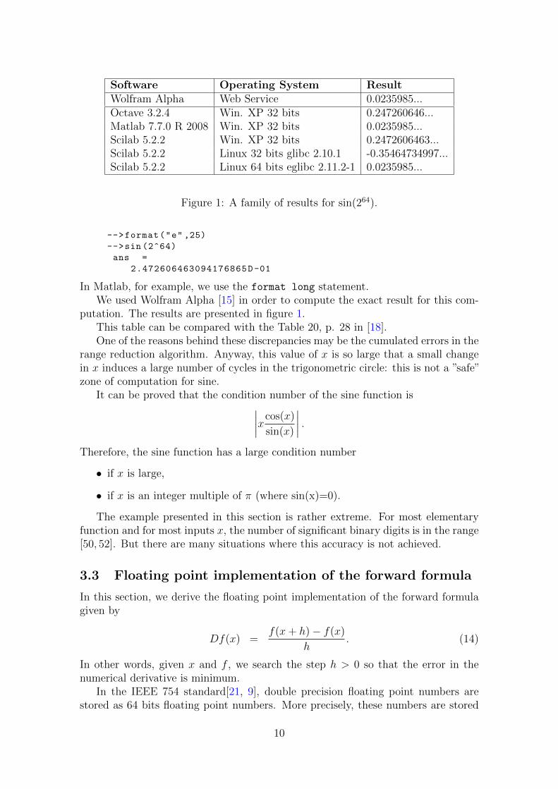
Software Operating System ResultWolfram Alpha Web Service 0.0235985...Octave 3.2.4 Win. XP 32 bits 0.247260646...Matlab 7.7.0 R 2008 Win. XP 32 bits 0.0235985...Scilab 5.2.2 Win. XP 32 bits 0.2472606463...Scilab 5.2.2 Linux 32 bits glibc 2.10.1 -0.35464734997...Scilab 5.2.2 Linux 64 bits eglibc 2.11.2-1 0.0235985...

Figure 1: A family of results for sin(264).

-->format("e" ,25)

-->sin (2^64)

ans =

2.472606463094176865D-01

In Matlab, for example, we use the format long statement.We used Wolfram Alpha [15] in order to compute the exact result for this com-

putation. The results are presented in figure 1.This table can be compared with the Table 20, p. 28 in [18].One of the reasons behind these discrepancies may be the cumulated errors in the

range reduction algorithm. Anyway, this value of x is so large that a small changein x induces a large number of cycles in the trigonometric circle: this is not a ”safe”zone of computation for sine.

It can be proved that the condition number of the sine function is∣∣∣∣xcos(x)

sin(x)

∣∣∣∣ .Therefore, the sine function has a large condition number

• if x is large,

• if x is an integer multiple of π (where sin(x)=0).

The example presented in this section is rather extreme. For most elementaryfunction and for most inputs x, the number of significant binary digits is in the range[50, 52]. But there are many situations where this accuracy is not achieved.

3.3 Floating point implementation of the forward formula

In this section, we derive the floating point implementation of the forward formulagiven by


h. (14)

In other words, given x and f , we search the step h > 0 so that the error in thenumerical derivative is minimum.

In the IEEE 754 standard[21, 9], double precision floating point numbers arestored as 64 bits floating point numbers. More precisely, these numbers are stored

10

with 52 bits in the mantissa, 1 sign bit and 11 bits in the exponent. In Scilab,which uses double precision numbers, the machine precision is stored in the globalvariable %eps, which is equal to εM = 1

252= 2.220.10−16. This means that, any

value x has 52 significants binary digits, corresponds to approximately 16 decimaldigits. If IEEE 754 single precision floating point numbers were used (i.e. 32 bitsfloating point numbers with 23 bits in the mantissa), the precision to use would beεM = 1

223≈ 10−7.

We can, as Dumontet and Vignes[6], consider the forward difference formula 7very closely. Indeed, there are many sources of errors which can be considered:

• the point x is represented in the machine by x,

• the step h is represented in the machine by h,

• the point x + h is computed in the machine as x ⊕ h, where the ⊕ operationis the addition,

• the function value of f at point x is computed by the machine as f(x),

• the function value of f at point x+h is computed by the machine as f(x⊕ h),

• the difference f(x+h)− f(x) is computed by the machine as f(x⊕ h) f(x),where the operation is the subtraction,

• the factor (f(x + h) − f(x))/h is computed by the machine as (f(x + h) f(x))� h, where the � operation is the division.

All in all, the forward difference formula


h(15)

is computed by the machine as

Df(x) = (f(x⊕ h) f(x))� h. (16)

For example, consider the error which is associated with the sum x ⊕ h. If thestep h is too small, the sum x⊕ h is equal to x. On the other side, if the step h istoo large then the sum x⊕ h is equal to h. We may require that the step h is in theinterval [2−52x, 252x] so that x are not too far away from each other in magnitude.We will discuss this assumption later in this chapter.

Dumontet and Vignes show that the most important source of error in the com-putation is the function evaluation. That is, the addition ⊕, subtraction anddivision � operations and the finite accuracy of x and h, produce most of the timea much lower relative error than the error generated by the function evaluation.

With a floating point computer, the total error that we get from the forwarddifference approximation 14 is (skipping the multiplication constants) the sum oftwo terms :

• the truncation error caused by the term h2f ′′(x),

11

• and the rounding error εM |f(x)| on the function values f(x) and f(x+ h).

Therefore, the error associated with the forward finite difference is

E(h) =εM |f(x)|

h+h

2|f ′′(x)| (17)

The total error is then the balance between the positive functions εM |f(x)|h

andh2|f ′′(x)|.• When h→∞, the error is dominated by the truncation error h

2|f ′′(x)|.

• When h→ 0, the error is dominated by the rounding error εM |f(x)|h

.

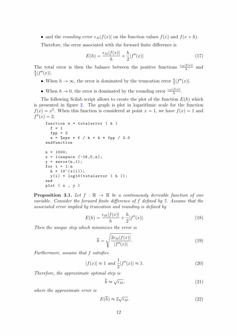
The following Scilab script allows to create the plot of the function E(h) whichis presented in figure 2. The graph is plot in logarithmic scale for the functionf(x) = x2. When this function is considered at point x = 1, we have f(x) = 1 andf ′′(x) = 2.

function e = totalerror ( h )

f = 1

fpp = 2

e = %eps * f / h + h * fpp / 2.0

endfunction

n = 1000;

x = linspace (-16,0,n);

y = zeros(n,1);

for i = 1:n

h = 10^(x(i));

y(i) = log10(totalerror ( h ));

end

plot ( x , y )

Proposition 3.1. Let f : R → R be a continuously derivable function of onevariable. Consider the forward finite difference of f defined by 7. Assume that theassociated error implied by truncation and rounding is defined by

E(h) =εM |f(x)|

h+h

2|f ′′(x)|. (18)

Then the unique step which minimizes the error is

h =

√2εM |f(x)||f ′′(x)|

. (19)

Furthermore, assume that f satisfies

|f(x)| ≈ 1 and1

2|f ′′(x)| ≈ 1. (20)

Therefore, the approximate optimal step is

h ≈√εM , (21)

where the approximate error is

E(h) ≈ 2√εM . (22)

12

log(h)

-14 -12 -10 -6 -0-8 -2

log(

E)

-16

1

0

-1

-2

-3

-4

-5

-6

-7

-8-4

Total error of numerical derivative

Figure 2: Total error of the numerical derivative as a function of the step in loga-rithmic scale - Theory.

13

Proof. The total error is minimized when the derivative of the function E is zero.The first derivative of the function E is

E ′(h) = −εM |f(x)|h2

+1

2|f ′′(x)|. (23)

The second derivative of E is

E ′′(h) = 2εM |f(x)|

h3. (24)

If we assume that f(x) 6= 0, then the second derivative E ′′(h) is strictly positive,since h > 0 (i.e. we consider only non-zero steps). This first derivative E ′(h) is zeroif and only if

− εM |f(x)|h2 +

1

2|f ′′(x)| = 0 (25)

Therefore, the optimal step is 19. If we make the additionnal assumptions 20, thenthe optimal step is given by 21. If we plug the equality 21 into the definition of thetotal error 17 and use the assumptions 20, we get the error as in 22, which concludesthe proof.

The previous analysis shows that a more robust algorithm to compute the nu-merical first derivative of a function of one variable is:

h = sqrt(%eps)

fp = (f(x+h)-f(x))/h

In order to evaluate f ′(x), two evaluations of the function f are required byformula 14 at points x and x + h. In practice, the computational time is mainlyconsumed by the evaluation of f . The practical computation of 21 involves only theuse of the elementary function

√., which is negligible.

In Scilab, we use double precision floating point numbers so that the roundingerror is

εM ≈ 10−16. (26)

We are not concerned here with the exact value of εM , since only the order ofmagnitude matters. Therefore, based on the simplified formula 21, the optimal stepassociated with the forward numerical difference is

h ≈ 10−8. (27)

This is associated with the approximate error

E(h) ≈ 2.10−8. (28)

14

3.4 Numerical experiments with the robust forward formula

We can introduce the accuracy of the function evaluation by modifying the equation19. Indeed, if we take into account for 12 and 13, we get:

h =

√2c(x)εM |f(x)||f ′′(x)|

(29)

=

√2c(x)|f(x)||f ′′(x)|

√εM . (30)

In pratice, it is, unfortunately, not possible to compute the optimum step. It is stillpossible to analyse what happens in simplified situations where the exact derivativeis known.

We now consider the function f(x) =√x, for x ≥ 0 and evaluate its numerical

derivative at the point x = 1. In the following Scilab functions, we define thefunctions f(x) =

√x, f ′(x) = 1/2x−1/2 and f ′′(x) = −1/4x−3/2.

function y = mysqrt ( x )

y = sqrt(x)

endfunction

function y = mydsqrt ( x )

y = 0.5 * x^( -0.5)

endfunction

function y = myddsqrt ( x )

y = -0.25 * x^( -1.5)

endfunction

The following Scilab functions define the approximate step h defined by h =√εM

and the optimum step h defined by 29.

function y = step_approximate ( )

y = sqrt(%eps)

endfunction

function y = step_exact ( f , fpp , x )

y = sqrt( 2 * %eps * abs(f(x)) / abs(fpp(x)))

endfunction

The following functions define the forward numerical derivative and the relativeerror. The relative error is not defined for points x so that f ′(x) = 0, but we willnot consider this situation in this experiment.

function y = forward ( f , x , h )

y = ( f(x+h) - f(x))/h

endfunction

function y = relativeerror ( f , fprime , x , h )

expected = fprime ( x )

computed = forward ( f , x , h )

y = abs ( computed - expected ) / abs( expected )

endfunction

The following Scilab functions plots the relative error for several steps h fromh = 10−16 to h = 1. The resulting data is plot in logarithmic scale.

function drawrelativeerror ( f , fprime , x , mytitle )

n = 1000

15

logharray = linspace (-16,0,n)

for i = 1:n

h = 10^( logharray(i))

logearray(i)=log10(relativeerror(f,fprime ,x,h))

end

plot ( logharray , logearray )

xtitle(mytitle ,"log(h)","log(E)")

endfunction

We now use the previous functions and execute the following Scilab statements.

x = 1.0;

drawrelativeerror ( mysqrt , mydsqrt , x ,

"Relative error of numerical derivative in x=1.0");

h1 = step_approximate ( );

mprintf ( "Step Approximate = %e\n", h1)

h2 = step_exact ( mysqrt , myddsqrt , x );

mprintf ( "Step Exact = %e\n", h2)

The previous script produces the following output:

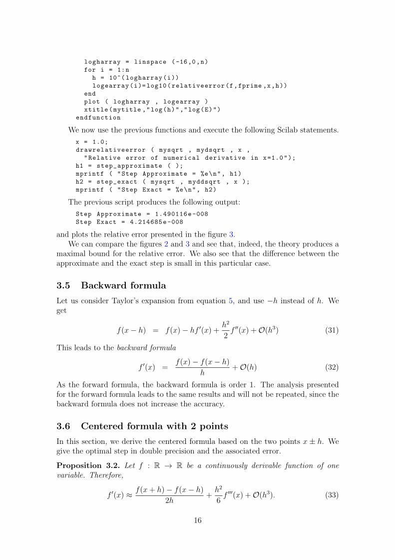
Step Approximate = 1.490116e-008

Step Exact = 4.214685e-008

and plots the relative error presented in the figure 3.We can compare the figures 2 and 3 and see that, indeed, the theory produces a

maximal bound for the relative error. We also see that the difference between theapproximate and the exact step is small in this particular case.

3.5 Backward formula

Let us consider Taylor’s expansion from equation 5, and use −h instead of h. Weget

f(x− h) = f(x)− hf ′(x) +h2

2f ′′(x) +O(h3) (31)

This leads to the backward formula

f ′(x) =f(x)− f(x− h)

h+O(h) (32)

As the forward formula, the backward formula is order 1. The analysis presentedfor the forward formula leads to the same results and will not be repeated, since thebackward formula does not increase the accuracy.

3.6 Centered formula with 2 points

In this section, we derive the centered formula based on the two points x ± h. Wegive the optimal step in double precision and the associated error.


f ′(x) ≈ f(x+ h)− f(x− h)

2h+h2

6f ′′′(x) +O(h3). (33)

16

log(h)

-14 -12 -10 -6 -0-8 -2

log(

E)

-16

-0

-2

-4

-6

-8

-10

-12-4

Relative error of numerical derivative in x=1.0

Figure 3: Total error of the numerical derivative as a function of the step in loga-rithmic scale - Numerical experiment.

17

Proof. The Taylor expansion of the function f at point x is

f(x+ h) = f(x) + hf ′(x) +h2

2f ′′(x) +

h3

6f ′′′(x) +O(h4). (34)

If we replace h by −h in the previous equation we get

f(x− h) = f(x)− hf ′(x) +h2

2f ′′(x)− h3

6f ′′′(x) +O(h4). (35)

We subtract the two equations 34 and 35 and get

f(x+ h)− f(x− h) = 2hf ′(x) +h3

3f ′′′(x) +O(h4). (36)

We immediately get 33, which concludes the proof, or, more simply, the centered 2points finite difference

f ′(x) =f(x+ h)− f(x− h)

2h+O(h2), (37)

which approximates f ′ at order 2.

Definition 3.3. ( Centered two points finite difference for f ′) The finite differenceformula

Df(x) =f(x+ h)− f(x− h)

2h(38)

is the centered 2 points finite difference for f ′ and is an order 2 approximation forf ′.

Proposition 3.4. Let f : R → R be a continuously derivable function of onevariable. Consider the centered 2 points finite difference of f defined by 38. Assumethat the total error implied by truncation and rounding is

E(h) =εM |f(x)|

h+h2

6|f ′′′(x)|. (39)

Therefore, the unique step which minimizes the error is

h =

(3r|f(x)||f ′′′(x)|

)1/3

. (40)

Assume that f satisfies

|f(x)| ≈ 1 and1

3|f ′′′(x)| ≈ 1. (41)

Therefore, the approximate step which minimizes the error is

h ≈ ε1/3M . (42)

which is associated with the approximate error

E(h) ≈ 3

2ε2/3M . (43)

18

Proof. The first derivative of the error is

E ′(h) = −εM |f(x)|h2

+h

3|f ′′′(x)|. (44)

The error is minimum when the first derivative of the error is zero

− εM |f(x)|h2 +

h2

3|f ′′′(x)| = 0. (45)

The solution of this equation is 40. By the hypothesis 41, the optimal step is givenby 42, which concludes the first part of the proof. If we plug the previous equalityinto the definition of the total error 39 and use the assumptions 41, we get the errorgiven by 43, which concludes the proof.

With double precision floating point numbers, the optimal step associated withthe centered numerical difference is

h ≈ 6.10−6. (46)

This is associated with the error

E(h) ≈ 5.10−11. (47)

3.7 Centered formula with 4 points

In this section, we derive the centered formula based on the fours points x± h andx± 2h. We give the optimal step in double precision and the associated error.


f ′(x) =8f(x+ h)− 8f(x− h)− f(x+ 2h) + f(x− 2h)

12h

+h4

30f (5)(x) +O(h5). (48)


f(x+ h) = f(x) + hf ′(x) +h2

2f (2)(x) +

h3

6f (3)(x) +

h4

24f (4)(x)

+h5

120f (5)(x) +O(h6). (49)


f(x− h) = f(x)− hf ′(x) +h2

2f (2)(x)− h3

6f (3)(x) +

h4

24f (4)(x)

− h5

120f (5)(x) +O(h6). (50)

19

We subtract the two equations 49 and 50 and get

f(x+ h)− f(x− h) = 2hf ′(x) +h3

3f (3)(x) +

h5

60f (5)(x) +O(h6). (51)

We replace h by 2h in the previous equation and get

f(x+ 2h)− f(x− 2h) = 4hf ′(x) +8h3

3f (3)(x) +

8h5

15f (5)(x) +O(h6). (52)

In order to eliminate the term f (3)(x), we multiply the equation 51 by 8 and get

8 (f(x+ h)− f(x− h)) = 16hf ′(x) +8h3

3f (3)(x) +

2h5

15f (5)(x) +O(h6). (53)

We subtract equations 52 and 53 and we have

8 (f(x+ h)− f(x− h))− (f(x+ 2h)− f(x− 2h))

= 12hf ′(x)− 6h5

15f (5)(x) +O(h6). (54)

We divide the previous equation by 12h and get

8 (f(x+ h)− f(x− h))− (f(x+ 2h)− f(x− 2h))

12h

= f ′(x)− h4

30f (5)(x) +O(h5), (55)

which implies the equation 48 or, more simply,

f ′(x) =8f(x+ h)− 8f(x− h)− f(x+ 2h) + f(x− 2h)

12h+O(h4), (56)

which is the centered 4 points formula of order 4.

Definition 3.6. ( Centered 4 points finite difference for f ′) The finite differenceformula

Df(x) =8f(x+ h)− 8f(x− h)− f(x+ 2h) + f(x− 2h)

12h(57)

is the centered 4 points finite difference for f ′.

Proposition 3.7. Let f : R → R be a continuously derivable function of onevariable. Consider the centered centered 4 points finite difference of f defined by 57.Assume that the total error implied by truncation and rounding is

E(h) =εM |f(x)|

h+h4

30|f (5)(x)|. (58)

Therefore, the optimal step is

h =

(15εM |f(x)|2|f (5)(x)|

)1/5

. (59)

20


|f(x)| ≈ 1 and2

15|f (5)(x)| ≈ 1, (60)

Therefore, the approximate step

h ≈ ε1/5M , (61)

which is associated with the error

E(h) ≈ 5

4ε4/5M . (62)


E ′(h) = −εM |f(x)|h2

+2h3

15|f (5)(x)|. (63)

The error is minimum when the first derivative of the error is zero

− εM |f(x)|h2 +

2h3

15|f (5)(x)| = 0. (64)

The solution of the previous equation is the step 59. If we make the assumptions 60,then the optimal step is 61, which concludes the first part of the proof. If we plugthe equality 61 into the definition of the total error 58 and use the assumptions 60,we get the error 62, which concludes the proof.

With double precision floating point numbers, the approximate optimal stepassociated with the centered 4 points numerical difference is

h ≈ 4.10−4. (65)

This is associated with the approximate error

E(h) ≈ 3.10−13. (66)

3.8 Some finite difference formulas for the first derivative

In this section, we present several formulas to compute the first derivative of afunction of several parameters. We present and compare the associated optimalsteps and optimal errors.

The figure 4 present various formulas for the computation of the first derivativeof a continuously derivable function f . The approximate optimum step h and theapproximate minimum error E(h) are computed for double precision floating pointnumbers. We do not take into account for the scaling with respect to x (see below).

The figure 5 present the optimal steps and the associated errors for various finitedifference formulas.

We notice that with increasing accuracy (i.e. with order from 1 to 4), the size ofthe step increases, while the error decreases.

21

Name Formula h

Forward 2 points f(x+h)−f(x)h

√εM

Centered 2 points f(x+h)−f(x−h)2h

ε1/3M

Centered 4 points −f(x+2h)+8f(x+h)−8f(x−h)+f(x−2h)12h

ε1/5M

Figure 4: Various formulas for the computation of the Jacobian of a given functionf .

Name h E(h)Forward 2 points 10−8 2.10−8

Centered 2 points 6.10−6 5.10−11

Centered 4 points 4.10−4 3.10−13

Figure 5: Optimal steps and error of finite difference formulas for the computationof the Jacobian of a given function f with double precision floating point numbers.We do not take into account for the scaling with respect to x.

3.9 A three points formula for the second derivative

In this section, we present a three points formula for the second derivative of afunction of one variable. We present the error analysis and compute the optimumstep and minimum error.


f ′′(x) =f(x+ h)− 2f(x) + f(x− h)

h2+h2

12f (4)(x) +O(h3). (67)


f(x+ h) = f(x) + hf ′(x) +h2

2f (2)(x) +

h3

6f (3)(x) +

h4

24f (4)(x)

+h5

120f (5)(x) +O(h6). (68)


f(x− h) = f(x)− hf ′(x) +h2

2f (2)(x)− h3

6f (3)(x) +

h4

24f (4)(x)

− h5

120f (5)(x) +O(h6). (69)

We sum the two equations 68 and 69 and get

f(x+ h) + f(x− h) = 2f(x) + h2f ′′(x) +h4

12f (4)(x) +O(h5). (70)

This leads to the three points finite difference formula 67, or, more simply,

f ′′(x) =f(x+ h)− 2f(x) + f(x− h)

h2+O(h2). (71)

22

The formula 71 shows that this three points finite difference is order 2.

Definition 3.9. ( Centered 3 points finite difference for f ′′) The finite differenceformula

Df(x) =f(x+ h)− 2f(x) + f(x− h)

h2(72)

is the centered 3 points finite difference for f ′′.

Proposition 3.10. Let f : R → R be a continuously derivable function of onevariable. Consider the centered centered 4 points finite difference of f defined by 72.Assume that the total error implied by truncation and rounding is

E(h) =εM |f(x)|

h2+h2

12|f (4)(x)|. (73)

Therefore, the unique step which minimizes the error is

h =

(12εM |f(x)||f (4)(x)|

)1/4

. (74)


|f(x)| ≈ 1 and1

12|f (4)(x)| ≈ 1, (75)

Therefore, the approximate step is

h ≈ ε1/4M , (76)

which is associated with the approximate error

E(h) ≈ 2ε1/2M . (77)


E ′(h) = −2r|f(x)|h3

+h

6|f (4)(x)|. (78)

Its second derivative is

E ′′(h) =6r|f(x)|h4

+1

6|f (4)(x)|. (79)

The second derivative is positive, since, by hypothesis, we have h > 0. Therefore,the function E is convex and has only one global minimum. The error E is minimumwhen the first derivative of the error is zero

− 2r|f(x)|h3 +

h

6|f (4)(x)| = 0. (80)

Therefore, the optimal step is given by the equation 74. By the hypothesis 75, theoptimal step is given by 76, which concludes the first part of the proof. If we plugthe equality 76 into the definition of the total error 73 and use the assumptions 75,we get the error 77, which concludes the proof.

23

With double precision floating point numbers, the optimal step associated withthe centered 4 points numerical difference is

h ≈ 1.10−4. (81)

This is associated with the error

E(h) = 3.10−8. (82)

3.10 Accuracy of finite difference formulas

In this section, we give a proposition which computes the order of magnitude ofmany finite difference formulas.

Proposition 3.11. Let f : R → R be a continuously derivable function of onevariable. We consider the derivative f (d), where d ≥ 1 is a positive integer. Assumethat the derivative f (d) is approximated by a finite difference formula. Assume thatthe rounding error associated with the finite difference formula is

Er(h) =εM |f(x)|

hd. (83)

Assume that the associated truncation error is

Et(h) =hp

β|f (d+p)(x)|, (84)

where β > 0 is a positive constant, p ≥ 1 is a strictly positive integer associatedwith the order of the finite difference formula. Therefore, the unique step whichminimizes the total error is

h =

(εM

d

pβ|f(x)||f (d+p)(x)|

) 1d+p

. (85)

Assume that the function f is so that

|f(x)| ≈ 1 and1

β|f (d+p)(x)| ≈ 1. (86)

Assume that the ratio d/p has an order of magnitude which is close to 1, i.e.

d

p≈ 1. (87)

Then the unique approximate optimal step is

h ≈ ε1

d+p

M , (88)

and the associated error is

E(h) ≈ 2εp

d+p

M . (89)

24

This proposition allows to compute the optimum step much faster than with acase by case analysis. The assumptions 86 might seem to be strong at first, but, aswe have allready seen, are reasonable in practice.

Proof. The total error is

E(h) =εM |f(x)|

hd+hp

β|f (d+p)(x)|. (90)

The first derivative of the error E is

E ′(h) = −dεM |f(x)|hd+1

+ php−1|f (d+p)(x)|

β. (91)

The second derivative of the error E is

E ′′(h) =

{d(d+ 1) εM |f(x)|

hd+2 , if p = 1

d(d+ 1) εM |f(x)|hd+2 + p(p− 1)hp−2 |f

(d+p)(x)|β

, if p ≥ 2(92)

Therefore, whatever the value of p ≥ 1, the second derivative of the error E ispositive. Hence, the function E is convex for h > 0. This implies that there is onlyone global minimum, which is the solution of the equation E ′(h) = 0. The optimumstep h satisfies the equation

− dεM |f(x)|hd+1

+ php−1 |f (d+p)(x)|

β= 0. (93)

This leads to the equation 85. Under the assumptions on the function f given by86 and on the factor d

pgiven by 87, the previous equality simplifies into

h = ε1

d+p

M , (94)

which proves the first result. The same assumptions simplify the approximate errorinto

E(h) ≈ εMhd

+ hp. (95)

If we introduce the optimal step 94 into the previous equation, we get

E(h) ≈ εM

εd

d+p

M

+ εp

d+p

M (96)

≈ εp

d+p

M + εp

d+p

M (97)

≈ 2εp

d+p

M , (98)


25

Example 3.1 Consider the following centered 3 points finite difference for f ′′

f ′′(x) =f(x+ h)− 2f(x) + f(x− h)

h2+h2

12f (4)(x) +O(h3). (99)

The error implied by truncation and rounding is

E(h) =εM |f(x)|

h2+h2

12|f (4)(x)|, (100)

which can be interpreted in the terms of the proposition 3.11 with d = 2, p = 2 andβ = 12. Then the unique approximate optimal step is

h ≈ ε14M , (101)

and the associated approximate error is

E(h) ≈ 2ε12M . (102)

This result corresponds to the proposition 3.10, as expected.

3.11 A collection of finite difference formulas

In this section, we present some finite difference formulas which compute variousderivatives with various orders of precision. For each formula, the optimum stepand the minimum error is presented, under the assumptions of the proposition 3.11.

• First derivative : forward 2 points

f ′(x) =f(x+ h)− f(x)

h+O(h) (103)

Optimal step : h ≈ ε1/2M and error E ≈ ε

1/2M .

Double precision h ≈ 10−8 and E ≈ 10−8.

• First derivative : backward 2 points

f ′(x) =f(x)− f(x− h)

h+O(h) (104)


1/2M .


• First derivative : centered 2 points

f ′(x) =f(x+ h)− f(x− h)

2h+O(h2) (105)

Optimal step : h = ε1/3M and error E ≈ ε

2/3M .


26

• First derivative : double forward 3 points

f ′(x) =−f(x+ 2h) + 4f(x+ h)− 3f(x)

2h+O(h2) (106)


2/3M .


• First derivative : double backward 3 points

f ′(x) =f(x− 2h)− 4f(x+ h) + 3f(x)

2h+O(h2) (107)


2/3M .


• First derivative : centered 4 points

f ′(x) =1

12h(−f(x+ 2h) + 8f(x+ h)

−8f(x− h) + f(x− 2h)) +O(h4) (108)


4/5M .


• Second derivative : forward 3 points

f ′′(x) =f(x+ 2h)− 2f(x+ h) + f(x)

h2+O(h) (109)


1/3M .


• Second derivative : centered 3 points

f ′′(x) =f(x+ h)− 2f(x) + f(x− h)

h2+O(h2) (110)


1/2M .


• Second derivative : centered 5 points

f ′′(x) =1

12h2(−f(x+ 2h) + 16f(x+ h)− 30f(x)

+16f(x− h)− f(x− 2h)) +O(h4) (111)


2/3M .


27

• Third derivative : centered 4 points

f (3)(x) =1

2h3(f(x+ 2h)− 2f(x+ h)+

2f(x− h)− f(x− 2h)) +O(h2) (112)


2/5M .


• Fourth derivative : centered 5 points

f (4)(x) =1

h2(f(x+ 2h)− 4f(x+ h) + 6f(x)

−4f(x− h) + f(x− 2h)) +O(h2) (113)


1/3M .


Some of the prevous formulas will be presented in the context of Scilab in thesection 4.3.

4 Finite differences of multivariate functions

In this section, we analyse methods to approximate the derivatives of multivariatefunctions with Scilab. In the first part, we present the gradient and Hesssian ofa multivariate function. Then we analyze methods to compute the derivatives ofmultivariate functions with finite differences. We present Scilab functions to com-pute these derivatives. By composing the finite difference operators, it is possible toapproximate higher degree derivatives and we present how to use this method withScilab. Finally, we present Richardson’s method to approximate derivatives withmore accuracy and discuss methods to take bounds into account.

4.1 Multivariate functions

In this section, we present formulas which allow to compute the numerical derivativesof multivariate function.

Assume that n is a positive integer representing the dimension of the space.Assume that f is a multivariate continuously differentiable function : f : Rn → R.We denote by x ∈ Rn the current vector with n dimensions. The n-vector of partialderivatives of f is the gradient of f and will be denoted by ∇f(x) or g(x):

∇f(x) = g(x) =

∂f∂x1...∂f∂xn

. (114)

Consider the function f : Rn → Rm, where m is a positive integer. Then thepartial derivatives form a n×m matrix, which is called the Jacobian matrix. In this

28

document, we will consider only the case m = 1, but the results which are presentedcan be applied directly to each component of f(x). Hence, the case m > 1 doesnot introduce any new problem and we will not consider it in the remaining of thisdocument.

Higher derivatives of a multivariate function are defined as in the univariatecase. Assume that f has continous partial derivatives ∂f/∂xi for i = 1, . . . , n andcontinous partial derivatives ∂2f/∂xi∂xj i, j = 1, . . . , n. Then the Hessian matrixof f is denoted by ∇2f(x) of H(x):

∇2f(x) = H(x) =

∂2f∂x21

. . . ∂2f∂x1∂xn

......

∂2f∂x1∂xn

. . . ∂2f∂x2n

. (115)

The Taylor-series expansion of a general function f in the neighbourhood of apoint x can be derived as in the univariate case presented in the section 2.1.1. Letx ∈ Rn be a given point, p ∈ Rn a vector of unit length and h ∈ R a scalar. Thefunction f(x + hp) can be regarded as a univariate function of h and the univariateexpansion can be applied directly:

f(x + hp) = f(x) + hg(x)Tp +1

2h2pTH(x)p + . . .

+1

(n− 1)!hn−1Dn−1f(x) +

1

n!hnDnf(x + θhp), (116)

for some θ ∈ [0, 1] and where

Dsf(x) =∑i1=1,n

∑i2=1,n

. . .∑is=1,n

pi1pi2 . . . pis∂sf(x)

∂xi1∂xi2 . . . ∂xis. (117)

We can expand Taylor’s formula, keep only the first three terms of this expansionand get:

f(x + hp) = f(x) + hg(x)Tp +1

2h2pTH(x)p +O(h3). (118)

The term hg(x)Tp is the directional derivative of f and is an order 1 term whichdrives the rate of change of f at the point x. The order 2 term pTH(x)p is thecurvature of f along p. A direction p such that ptH(x)p > 0 is termed a directionof positive curvature.

In the particular case of a function of two variables, the previous general formula

29

can be written in integral form:

f(x1 + h1, x2 + h2) = f(x1, x2) + h1∂f

∂x1+ h2

∂f

∂x2

+h212

∂2f

∂x21+ h1h2

∂2f

∂x1∂x2+h222

∂2f

∂x22

+h316

∂3f

∂x31+h21h2

2

∂3f

∂x21∂x2+h1h

22

2

∂3f

∂x1∂x22+h326

∂3f

∂x32

+h4124

∂4f

∂x41+h31h2

6

∂4f

∂x41∂x2+h21h

22

4

∂4f

∂x21∂x22

+h1h

32

6

∂4f

∂x1∂x32+h4224

∂4f

∂x42+ . . .

+∑

m+n=p

hm1m!

hn2n!

∫ 1

0

∂pf

∂xm1 ∂xn2

(x1 + th1, x2 + th2)p(1− t)p−1dt, (119)

where the terms associated with the partial derivates of degree p have the form∑m+n=p

hm1m!

hn2n!

∂pf

∂xm1 ∂xn2

. (120)

4.2 Numerical derivatives of multivariate functions

The Taylor-series expansion of a general function f allows to derive approximationof the function in a neighbourhood of x. Indeed, if we keep the first term in theexpansion, we get

f(x + hp) = f(x) + hg(x)Tp +O(h2). (121)

This formula leads to an order 1 finite difference formula for the multivariatefunction f . We emphasize that the equation 121 is an univariate expansion in thedirection p. This is why the univariate finite difference formulas can be directlyapplied for multivariate functions. Let hi be the step associated with the i-th com-ponent of x, and let ei ∈ Rn be the vector ei = ((ei)1, (ei)2, . . . , (ei)n)T with

(ei)j =

{1 if i = j,0 if i 6= j,

(122)

for j = 1, . . . , n. Then,

f(x + hiei) = f(x) + hig(x)Tei +O(h2). (123)

The term g(x)Tei is the i-th component of the gradient g(x), so that g(x)Tei =gi(x). Therefore, we can approximate the gradient of the function f by the finitedifference formula

gi(x) =f(x + hiei)− f(x)

hi+O(h). (124)

The previous formula is a multivariate finite difference formula of order 1 for thegradient of the function f . It is the direct analog of univariate finite differencesformulas that we have previously analyzed.

30

Similarily to the univariate case, the centered 2 points multivariate finite differ-ence for the gradient of f is

gi(x) =f(x + hiei)− f(x− hiei)

hi+O(h2) (125)

and the centered 4 points multivariate finite difference for the gradient of f is

gi(x) =8f(x + hiei)− 8f(x− hiei)− f(x + 2hiei) + f(x− 2hiei)

12hi+O(h4). (126)

We have alread noticed that the previous formulas are simply the univariateformula in the direction hiei. The consequence is that the evaluation of the gradientvector g requires n univariate finite differences.

4.3 Derivatives of a multivariate function in Scilab

In this section, we present a function which computest the Jacobian of a multivariatefunction f .

The following derivativeJacobianStep function computes the approximate op-timal step for some of the formulas for the first derivative. The function takes theformula name form as input argument and returns the approximate (scalar) optimalstep h.

function h = derivativeJacobianStep(form)

select form

case "forward2points" then // Order 1

h=%eps ^(1/2)

case "backward2points" then // Order 1

h=%eps ^(1/2)

case "centered2points" then // Order 2

h=%eps ^(1/3)

case "doubleforward3points" then // Order 2

h=%eps ^(1/3)

case "doublebackward3points" then // Order 2

h=%eps ^(1/3)


h=%eps ^(1/5)

else

error(msprintf("Unknown formula %s",form))

end

endfunction

The following derivativeJacobian function computes an approximate Jaco-bian. It takes as input argument the function f, the vector point x, the vector steph and the formula form and returns the approximate Jacobian J.

function J = derivativeJacobian(f,x,h,form)

n = size(x,"*")

D = diag(diag(h))

for i = 1 : n

d = D(:,i)

select form


31

J(i) = (f(x+d)-f(x))/h(i)


J(i) = (f(x)-f(x-d))/h(i)


J(i) = (f(x+d)-f(x-d))/(2*h(i))


J(i) = (-f(x+2*d)+4*f(x+d)-3*f(x))/(2*h(i))


J(i) = (f(x-2*d)-4*f(x-d)+3*f(x))/(2*h(i))


J(i) = (-f(x+2*d) + 8*f(x+d)..

-8*f(x-d)+f(x-2*d))/(12*h(i))

else


end

end

endfunction

In the previous function, the statement D=diag(h) creates a diagonal matrix D

where the diagonal entries are equal to the vector h. Therefore, the i-th column ofD is equal to hiei, as defined in the previous section.

We now experiment our approximate Jacobian function. The following functionquadf computes a quadratic function.

function f = quadf ( x )

f = x(1)^2 + x(2)^2

endfunction

The quadJ function computes the exact Jacobian of quadf.

function J = quadJ ( x )

J(1) = 2 * x(1)

J(2) = 2 * x(2)

endfunction

In the following session, we compute the exact Jacobian matrix at the point x =(1, 2)T .

-->x=[1;2];

-->J = quadJ ( x )

J =

2.

4.

In the following session, we compute the approximate Jacobian matrix at the pointx = (1, 2)T .

-->form = "forward2points";

-->h = derivativeJacobianStep(form)

h =

0.0007401

-->h = h*ones (2,1)

h =

0.0007401

0.0007401

-->Japprox = derivativeJacobian(quadf ,x,h,form)

Japprox =

2.

4.

32

Although the derivativeJacobian function has interesting features, there aresome limitations.

• We cannot compute the Jacobian matrix of a function which returns a m-by-1vector: only scalar functions can be differentiated.

• We cannot differentiate a function f which requires extra-arguments.

Both these limitations are addressed in the next section.

4.4 Derivatives of a vectorial function with Scilab

In this section, we present a Scilab script which computes the Jacobian matrix of avectorial function. This script will be used in the section 4.6,

where we compose derivatives.In order to manage extra-arguments, we will make so that the function to be

differentiated can be either

• a function, with calling sequence y=f(x),

• a list (f,a1,a2,...). In this case, the first element in the list is the function tobe differentiated with calling sequence y=f(x,a1,a2,...), and the remainingarguments a1,a2,... are automatically appended to the calling sequence.

Both cases are managed by the following derivativeEvalf function, which evalu-ates the function __derEvalf__ at the given point x.

function y = derivativeEvalf(__derEvalf__ ,x)

if ( typeof(__derEvalf__ )=="function" ) then

y = __derEvalf__(x)

elseif ( typeof(__derEvalf__ )=="list" ) then

__f_fun__ = __derEvalf__ (1)

y = __f_fun__(x,__derEvalf__ (2:$))

else

error(msprintf("Unknown function type %s",typeof(f)))

end

endfunction

The complicated name __derEvalf__ has been chosen in order to avoid conflictsbetween the name of the argument and the name of the user-defined function. In-deed, such a conflict may produce an infinite recursion. This topic is presented inmore depth in [5].

The following derivativeJacobian function computes the Jacobian matrix ofa given function __derJacf__.

function J = derivativeJacobian(__derJacf__ ,x,h,form)

n = size(x,"*")

D = diag(h)

for i = 1 : n

d = D(:,i)

select form


y(:,1) = -derivativeEvalf(__derJacf__ ,x)

y(:,2) = derivativeEvalf(__derJacf__ ,x+d)

33


y(:,1) = derivativeEvalf(__derJacf__ ,x)

y(:,2) = -derivativeEvalf(__derJacf__ ,x-d)


y(:,1) = 1/2* derivativeEvalf(__derJacf__ ,x+d)

y(:,2) = -1/2* derivativeEvalf(__derJacf__ ,x-d)


y(:,1) = -3/2* derivativeEvalf(__derJacf__ ,x)

y(:,2) = 2* derivativeEvalf(__derJacf__ ,x+d)

y(:,3) = -1/2* derivativeEvalf(__derJacf__ ,x+2*d)


y(:,1) = 3/2* derivativeEvalf(__derJacf__ ,x)

y(:,2) = -2* derivativeEvalf(__derJacf__ ,x-d)

y(:,3) = 1/2* derivativeEvalf(__derJacf__ ,x-2*d)


y(:,1) = -1/12* derivativeEvalf(__derJacf__ ,x+2*d)

y(:,2) = 2/3* derivativeEvalf(__derJacf__ ,x+d)

y(:,3) = -2/3* derivativeEvalf(__derJacf__ ,x-d)

y(:,4) = 1/12* derivativeEvalf(__derJacf__ ,x-2*d)

else


end

J(:,i) = sum(y,"c")/h(i)

end

endfunction

The following quadf function takes as input argument a 3-by-1 vector and returnsa 2-by-1 vector.

function y = quadf ( x )

f1 = x(1)^2 + x(2)^3 + x(3)^4

f2 = exp(x(1)) + 2*sin(x(2)) + 3*cos(x(3))

y = [f1;f2]

endfunction

The quadJ function returns the Jacobian matrix of quadf.

function J = quadJ ( x )

J1(1) = 2 * x(1)

J1(2) = 3 * x(2)^2

J1(3) = 4 * x(3)^3

//

J2(1) = exp(x(1))

J2(2) = 2*cos(x(2))

J2(3) = -3*sin(x(3))

//

J = [J1 ’;J2 ’]

endfunction

In the following session, we compute the exact Jacobian matrix of quadf at thepoint x = (1, 2, 3)T .

-->x=[1;2;3];

-->J = quadJ ( x )

J =

2. 12. 108.

2.7182818 - 0.8322937 - 0.4233600

34

In the following session, we compute the approximate Jacobian matrix of the functionquadf.

-->x=[1;2;3];

-->form = "forward2points";

-->h = derivativeJacobianStep(form);

-->h = h*ones (3,1);

-->Japprox = derivativeJacobian(quadf ,x,h,form)

Japprox =

2. 12. 108.

2.7182819 - 0.8322937 - 0.4233600

4.5 Computing higher degree derivatives

In this section, we present a result which allows to get a finite difference operatorfor f ′′, based on a finite difference operator for f ′.

Consider the 2 points forward finite difference operator Df defined by


h, (127)

which produce an order 1 approximation for f ′. Similarily, let us consider the finitedifference operator DDf defined by

DDf(x) =Df(x+ h)−Df(x)

h, (128)

that is, the composed operator DDf = (D ◦ D)f . It would be nice if DD was anapproximation for f ′′. The previous formula simplifies into

DDf(x) =f(x+2h)−f(x+h)

h− f(x+h)−f(x)

h

h(129)

=f(x+ 2h)− f(x+ h)− f(x+ h) + f(x)

h2(130)

=f(x+ 2h)− 2f(x+ h) + f(x)

h2. (131)

It is straightforward to prove that the previous formula is, indeed, an order 1 formulafor f ′′, that is, DDf defined by 128 is an order 1 approximation for f ′′. The followingproposition presents this result in a more general framework.

Proposition 4.1. Let f : R → R be a continuously derivable function of onevariable. Let Df be a finite difference operator of order p > 0 for f ′. Therefore thefinite difference operator DDf is of order p for f ′′.

Proof. By hypothesis, Df is of order p, which implies that

Df(x) = f ′(x) +O(hp). (132)

Let us define g by

g(x) = Df(x). (133)

35

Since f is continuously derivable function, so is g. Therefore, Dg is of order p forg′, which implies

Dg(x) = g′(x) +O(hp). (134)

We now plug the definition of g given by 133 into the previous equation and get

DDf(x) = (Df)′(x) +O(hp) (135)

= f ′′(x) +O(hp), (136)


Example 4.1 Consider the centered 2 points finite difference for f ′ defined by

Df(x) =f(x+ h)− f(x− h)

2h. (137)

We have proved in proposition 3.2 that Df is an order 2 approximation for f ′. Wecan therefore apply the proposition 4.1 with p = 2 and get an approximation for f ′′

based on the finite difference

DDf(x) =Df(x+ h)−Df(x− h)

2h. (138)

We can expand this formula and get

DDf(x) =f(x+2h)−f(x)

2h− f(x)−f(x−2h)

2h

2h(139)

=f(x+ 2h)− 2f(x) + f(x− 2h)

4h2, (140)

which is, by proposition 4.1 a finite difference formula of order 2 for f ′′.In practice, it may not be required to expand the finite difference in the way

of 139. Indeed, Scilab can manage callbacks (i.e. function pointers), so that it iseasy to use the proposition 4.1 so that the computation of the second derivativeis performed with the same source code that for the first derivative. This methodis used in the derivative function of Scilab, as we will see in the correspondingsection.

We may ask if, by chance, a better result is possible for the finite difference DD.More precisely, we may ask if the order of the operator DD may be greater than theorder of the operator D. In fact, there is no better result, as we are going to see. Inorder to analyse if a higher order formula would be produced, we must explicitelywrite higher order terms in the finite difference approximation. Let us write thefinite difference operator Df by

Df(x) = f ′(x) +hp

βf (d+p)(x) +O(hp+1), (141)

where β > 0 is a positive real and d ≥ 1 is an integer. We have

DDf(x) = (Df)′(x) +hp

β(Df)(d+p)(x) +O(hp+1) (142)

=

(f ′′(x) +

hp

βf (d+p+1)(x) +O(hp+1)

)+hp

β

(f (d+p+1)(x) +

hp

βf (2d+2p)(x) +O(hp+1)

)+O(hp+1). (143)

36

Hence

DDf(x) = f ′′(x) + 2hp

βf (d+p+1)(x) +

h2p

β2f (2d+2p)(x) +O(hp+1). (144)

We can see that the second term in the expansion is 2hp

βf (d+1)(x), which is of order

p. There is no assumption which may set this term to zero, which implies that DDis of order p, at best.

Of course, the process can be extended in order to compute more derivatives.Suppose that we want to compute an approximation for f (d)(x), where d ≥ 1 is aninteger. Let us define the finite difference operator D(d)f by recurrence on d as

D(d+1)f(x) = D ◦D(d)f(x). (145)

By proposition 4.1, if Df is a finite difference operator of order p for f ′, thereforeD(d)f is a finite difference operator of order p for f (d)(x).

We present how to implement the previous composition formulas in the section4.6. But, for reasons which will be made clear later in this document, we must firstconsider derivatives of multivariate functions and derivatives of vectorial functions.

4.6 Nested derivatives with Scilab

In this section, we present how to compute higher derivatives with Scilab, based onrecursive calls.

We consider the same functions which were defined in the section 4.4.The following derivativeHessianStep function returns the approximate opti-

mal step for the second derivative, depending on the finite difference formula form.

function h = derivativeHessianStep(form)

select form


h=%eps ^(1/3)


h=%eps ^(1/3)


h=%eps ^(1/4)


h=%eps ^(1/4)


h=%eps ^(1/4)


h=%eps ^(1/6)

else


end

endfunction

We define a function which returns the Jacobian matrix as a column vector.Moreover, we have to create a function with a calling sequence which is compatiblewith the one required by derivativeJacobian. The following derivativeFunc-

tionJ function returns the Jacobian matrix at the point x.

37

function J = derivativeFunctionJ(x,f,h,form)

J = derivativeJacobian(f,x,h,form)

J = J’

J = J(:)

endfunction

Notice that the arguments x and f are switched in the calling sequence. The followingsession shows how the derivativeFunctionJ function changes the shape of J.

-->x=[1;2;3];

-->H = quadH ( x );

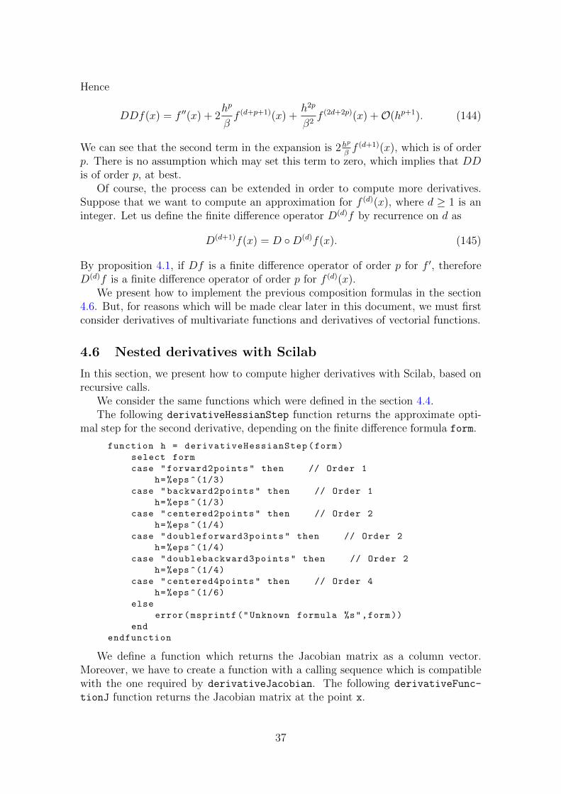
-->h = derivativeHessianStep("forward2points");

-->h = h*ones (3,1);

-->Japprox = derivativeFunctionJ(x,quadf ,h,form)

Japprox =

2.0000061

12.000036

108.00033

2.7182901

- 0.8322992

- 0.4233510

The following quadH function returns the Hessian matrix of the quadf function,which was defined in the section 4.4.

function H = quadH ( x )

H1 = [

2 0 0

0 6*x(2) 0

0 0 12*x(3)^2

]

//

H2 = [

exp(x(1)) 0 0

0 -2*sin(x(2)) 0

0 0 -3*cos(x(3))

]

//

H = [H1;H2]

endfunction

In the following session, we compute the Hessian matrix at the point x = (1, 2, 3)T .

-->x=[1;2;3];

-->H = quadH ( x )

H =

2. 0. 0.

0. 12. 0.

0. 0. 108.

2.7182818 0. 0.

0. - 1.8185949 0.

0. 0. 2.9699775

Notice that the rows #1 to #3 contain the Hessian matrix of the first component ofquadf, while the rows #4 to #6 contain the Hessian matrix of the second componentof quadf.

In the following session, we compute the approximate Hessian matrix of quadf.We use the approximate optimal step and the derivativeJacobian function, which

38

was defined in the section 4.4. The trick is that we differentiate derivativeFunc-

tionJ, instead of quadf.

-->h = derivativeHessianStep("forward2points");

-->h = h*ones (3,1);

-->funlist = list(derivativeFunctionJ ,quadf ,h,form);

-->Happrox = derivativeJacobian(funlist ,x,h,form)

Happrox =

1.9997533 0. 0.

0. 12.00007 0.

0. 0. 108.00063

2.7182693 0. 0.

0. - 1.8185741 0.

0. 0. 2.9699582

Although the previous method seems interesting, it has a major drawback: itdoes not exploit the symmetry of the Hessian matrix, so that the number of functionevaluations is larger than required. Indeed, the Hessian matrix of a smooth functionf is symmetric, i.e.

Hij = Hji, (146)

for i, j = 1, 2, . . . , n. This relation comes as a consequence of the equality

∂2f

∂xi∂xj=

∂2f

∂xj∂xi, (147)

for i, j = 1, 2, . . . , n.The symmetry implies that only the coefficients for which i ≥ j, for example,

need to be computed: the coefficients i < j can be deduced by symmetry of theHessian matrix. But the method that we have presented ignores this property. Thisleads to a number of function evaluations which could be divided roughly by a factor2.

4.7 Computing derivatives with more accuracy

In this section, we present a method to compute derivatives with more accuracy.This method, known as Richardson’s extrapolation, improves the accuracy by usinga sequence of steps with decreasing sizes.

We may ask if there is a general method to get a increased accuracy for a givenderivative, from an existing finite difference formula. Of course, such a finite differ-ence will require more function evaluations, which is the price to pay for an increasedaccuracy. The following proposition gives such a method.

Proposition 4.2. Assume that the finite difference operator Df approximates thederivative f (d) at order p > 0 where d, p ≥ 1 are integers. Assume that

Dfh(x) = f (d)(x) +hp

βf (d+p)(x) +O(hq), (148)

where β > 0 is a real constant and q is an integer greater than p. Therefore, thefinite difference operator

Df(x) =2pDfh(x)−Df2h(x)

2p − 1(149)

39

is an order q approximation for f (d).

Proof. The proof is based on a direct use of the equation 148, with different stepsh. With 2h instead of h in 148, we have

Df2h(x) = f (d)(x) +2p

βhpf (d+p)(x) +O(hq). (150)

We multiply the equation 148 by 2p and get:

2pDfh(x) = 2pf (d)(x) +2p

βhpf (d+p)(x) +O(hq), (151)

We subtract the equation 151 and the equation 150, and get

2pDfh(x)−Df2h(x) = (2p − 1)f (d)(x) +O(hq). (152)

We divide both sides of the previous equation by 2p−1 and get 149, which concludesthe proof.

Example 4.2 Consider the following centered 2 points finite difference operator forf ′

Dfh(x) =f(x+ h)− f(x− h)

2h. (153)

We have proved in proposition 3.2 that this is an approximation for f ′(x) and

Dfh(x) = f ′(x) +h2

6f (3)(x) +O(h4). (154)

Therefore, we can apply the proposition 4.2 with d = 1, p = 2, β = 6 and q = 4.Hence, the finite difference operator

Df(x) =4Dfh(x)−Df2h(x)

3(155)

is an order q = 4 approximation for f ′(x). We can expand this new finite differenceformula and find that we already have analysed it. Indeed, if we plug the definitionof the finite difference operator 153 into 155, we get

Df(x) =4f(x+h)−f(x−h)

2h− f(x+2h)−f(x−2h)

4h

3(156)

=8 (f(x+ h)− f(x− h))− (f(x+ 2h)− f(x− 2h))

12h. (157)

The previous finite difference operator is the one which has been presented in propo-sition 3.5, which states that it is an order 4 operator for f ′.

The problem with the proposition 4.2 is that the optimal step is changed. Indeed,since the order of the modified finite difference method is changed, therefore, theoptimal step is changed too. In this case, the proposition 3.11 can be applied tocompute an approximate optimal step.

40

4.8 Taking into account bounds on parameters

The backward formula might be useful in some practical situations where the param-eters are bounded. This might happen when this parameter represents a physicalquantity which is physically bounded. For example, the real parameter x mightrepresent a fraction which is naturally in the interval [0, 1].

Assume that some parameter x is bounded in a given interval [a, b], with a, b ∈ Rand a < b. Assume that the step h is given, may be by the formula 21. If b > a+h,there is no problem at computing the numerical derivative with the forward formula

f ′(a) ≈ f(a+ h)− f(a)

h. (158)

If we want to compute the numerical derivative at b with the forward formula

f ′(b) ≈ f(b+ h)− f(b)

h, (159)

this leads to a problem, since b + h /∈ [a, b]. In fact, any point x in the interval[b− h, b] leads to the problem. For such points, the backward formula may be usedinstead.

5 The derivative function

In this section, we present the derivative function. We present the main featuresof this function and show how to change the order of the finite difference method.We analyze of an orthogonal matrix may be used to change the directions of differ-entiation. Finally, we analyze the performances of derivative, in terms of functionevaluations.

5.1 Overview

The derivative function computes the Jacobian and the Hessian matrix of a givenfunction. We can use formulas of order 1, 2 or 4. Finally, the user can set the stepused in the finite difference formula. In this section, we will analyse all these points.

The following is the complete calling sequence for the derivative function.

[ J , H ] = derivative ( F , x , h , order , H_form , Q )

where the variables are

• J, the Jacobian vector,

• H, the Hessian matrix,

• F, the multivariate function,

• x, the current point,

• order, the order of the formula (1, 2 or 4),

• H_form, the Hessian matrix storage (’default’, ’blockmat’ or ’hypermat’),

41

• Q, a matrix used to scale the step.

Since we are concerned here by numerical issues, we will use the ”blockmat”Hessian matrix storage.

The order 1, 2 and 4 formulas for the Jacobian matrix are implemented withformulas similar to the ones presented in figure 4, that is, the computations arebased on forward 2 points (order 1), centered 2 points (order 2) and centered 4points (order 4) formulas. The approximate optimal step h is computed dependingon the formulas in order to minimize the total error.

The derivative function takes into account for multivariate functions, so thatall points which have been detailed in section 4.2 can be applied here. In particular,the function uses modified versions 124, 125 and 126. Indeed, instead of using onestep hi for each direction i = 1, . . . , n, the same step h is used for all components.

5.2 Varying order to check accuracy

Since several accuracy are provided by the derivative function, it is easy and usefulto check the accuracy of a specific numerical derivative. If the derivative varies onlyslightly with various formula orders, that implies that the user can be confidentin its derivatives. Instead, if the numerical derivatives varies greatly with differentformulas, that implies that the numerical derivative must be used with caution.

In the following Scilab script, we use various formulas to check the numericalderivative of the univariate quadratic function f(x) = x2.

function y = myfunction3 (x)

y = x^2;

endfunction

x = 1.0;

expected = 2.0;

for o = [1 2 4]

fp = derivative(myfunction3 ,x, order = o);

err = abs(fp -expected )/abs(expected );

mprintf("Order = %d, Relative error : %e\n",order ,err)

end

The previous script produces the following output, where the relative error isprinted.

Order = 1, Relative error : 7.450581e-009

Order = 2, Relative error : 8.531620e-012

Order = 4, Relative error : 0.000000e+000

Increasing the order produces increasing accuracy, as expected in such a simplecase.

An advanced feature is provided by the derivative function, namely the trans-formation of the directions by an orthogonal matrix Q. This is the topic of thefollowing section.

5.3 Orthogonal matrix

In this section, we describe the mathematics behind the orthogonal n×n matrix Q,which is an optionnal input argument of the derivative function. An orthogonal

42

matrix is a square matrix satisfying QT = Q−1.In order to simplify the discussion, let us assume that the function is a multi-

variate scalar function, i.e. f : Rn → R. Second, we want to produce a result whichdoes not explicitely depends on the canonical vectors ei. The goal is to be able tocompute directionnal derivatives in directions which are combinations of the axisvectors. Then, Taylor’s expansion in the direction Qei yields

f(x + hQei) = f(x) + hg(x)TQei +O(h2). (160)

This leads to

g(x)TQei =f(x + hQei)− f(x)

h. (161)

Recall that in the classical formula, the term g(x)Tei can be simplified into gi(x).But now, the matrix Q has been inserted in between, so that the direction is indeeddifferent. Let us denote by qi ∈ Rn the i-th column of the matrix Q. Let us denoteby dT ∈ Rn the row vector of function differences defined by

di =f(x + hQei)− f(x)

h(162)

for i = 1, . . . , n. The equation 161 is transformed into g(x)Tqi = di, or, in matrixform,

g(x)TQ = dT . (163)

We right multiply the previous equation by QT and get

g(x)TQQT = dTQT . (164)

By the orthogonality property of Q, this implies

g(x)T = dTQT . (165)

Finally, we transpose the previous equation and get

g(x) = Qd. (166)

The Hessian matrix can be computed based on the method which has beenpresented in the section 4.5. Hence, the computation of the Hessian matrix can alsobe modified to take into account the orthogonal matrix Q.

Let us consider the case where the function f : Rn → Rm, where m is a positiveinteger. We want to compute the Jacobian m× n matrix J defined by

J =

∂f1∂x1

. . . ∂f1∂xn

......

∂fm∂x1

. . . ∂fm∂xn

. (167)

In this case, the finite differences are defining a column vector, so that we mustconsider the m× n matrix D with entries

Dij =fi(x + hQej)− fi(x)

h, (168)

for i = 1, . . . ,m and j = 1, . . . , n. The Jacobian matrix J is therefore computedfrom

J = DQT . (169)

43

Degree Order EvaluationsJacobian 1 n+ 1Jacobian 2 2nJacobian 4 4nHessian 1 (n+ 1)2

Hessian 2 4n2

Hessian 4 16n2

Figure 6: The number of function evaluations for the Jacobian and Hessian matrices.

5.4 Performance of finite differences

In this section, we analyse the number of function evaluations required by the com-putation of the Jacobian and Hessian matrices with the derivative function.

The number of function evaluations required to perform the computation dependson the dimension n and the number of points in the formula. The table 6 summarizesthe results.

The following list analyzes the number of function evaluations required to com-pute the gradient of the function depending on the dimension and the order of theformula.

• The order = 1 formula requires n+1 function evaluations. Indeed, the functionmust be evaluated at f(x) and f(x + hei), for i = 1, . . . , n.

• The order = 2 formula requires 2n function evaluations. Indeed, the functionmust be evaluated at f(x− hei) and f(x + hei), for i = 1, . . . , n.

• The order = 4 formula requires 4n function evaluations. Indeed, the functionmust be evaluated at f(x− hei), f(x + hei), f(x− 2hei) and f(x + 2hei), fori = 1, . . . , n.

Consider the quadratic function in n = 10 dimensions

f(x) =∑i=1,10

x2i . (170)

In the following Scilab script, we define the function and use a global variable tostore the number of function evaluations required by the derivative function.


global nbfeval

nbfeval = nbfeval + 1

y = x.’ * x;

endfunction

x = (1:10). ’;

for o = [1 2 4]

global nbfeval

nbfeval = 0;

J = derivative(myfunction3 ,x,order=o);

mprintf("Order = %d, Feval : %d\n",o,nbfeval)

end

44

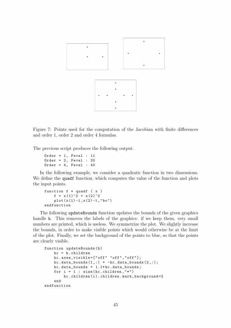
Figure 7: Points used for the computation of the Jacobian with finite differencesand order 1, order 2 and order 4 formulas.

The previous script produces the following output.

Order = 1, Feval : 11



In the following example, we consider a quadratic function in two dimensions.We define the quadf function, which computes the value of the function and plotsthe input points.

function f = quadf ( x )

f = x(1)^2 + x(2)^2

plot(x(1)-1,x(2)-1,"bo")

endfunction

The following updateBounds function updates the bounds of the given graphicshandle h. This removes the labels of the graphics: if we keep them, very smallnumbers are printed, which is useless. We symmetrize the plot. We slightly increasethe bounds, in order to make visible points which would otherwise be at the limitof the plot. Finally, we set the background of the points to blue, so that the pointsare clearly visible.

function updateBounds(h)

hc = h.children

hc.axes_visible =["off" "off","off"];

hc.data_bounds (1,:) = -hc.data_bounds (2,:);

hc.data_bounds = 1.1*hc.data_bounds;

for i = 1 : size(hc.children ,"*")

hc.children(i). children.mark_background =2

end

endfunction

45

Figure 8: Points used in the computation of the Hessian with finite differences andorder 1, order 2 and order 4 formulas. The points clustered in the middle are fromthe numerical Jacobian.

Then, we make several calls to the derivative function, which creates the plotswhich are presented in figures 7 and 8.

// See pattern for Jacobian

h = scf();

J1 = derivative(quadf ,x,order=1 );

updateBounds(h);

scf();


updateBounds(h);

scf();


updateBounds(h);

// See pattern for Hessian for order 2

h = scf();

[J1 , H1] = derivative(quadf ,x,order =1 );

updateBounds(h);

h = scf();


updateBounds(h);

h = scf();


updateBounds(h);

In the following example, we compute both the gradient and the Hessian matrixin the same case as previously.


global nbfeval

nbfeval = nbfeval + 1

y = x.’ * x;

endfunction

46

x = (1:10). ’;

for o = [1 2 4]

global nbfeval

nbfeval = 0;

[ J , H ] = derivative(myfunction3 ,x,order=o);

mprintf("Order = %d, Feval : %d\n",o,nbfeval)

end

The previous script produces the following output. Notice that, since we computeboth the gradient and the Hessian matrix, the number of function evaluations is thesum of the two, although, in practice, the cost of the Hessian matrix is the mostimportant.




6 One more step

In this section, we analyse the behaviour of derivative when the point x is eitherlarge x → ∞, when x is small x → 0 and when x = 0. We compare these resultswith the numdiff function, which does not use the same step strategy. As we aregoing to see, both commands performs the same when x is near 1, but performs verydifferently when x is large or small.

We have allready explained the theory of the floating point implementation ofthe derivative function. Is it completely bulletproof ? Not exactly.

See for example the following Scilab session, where one computes the numericalderivative of f(x) = x2 for x = 10−100. The expected result is f ′(x) = 2.× 10−100.

-->function y = myfunction (x)

--> y = x*x;

-->endfunction

-->fp = derivative(myfunction ,1.e-100, order =1)

fp =

0.0000000149011611938477

-->fe=2.e-100

fe =

2.000000000000000040 -100

-->e = abs(fp-fe)/fe

e =

7.450580596923828243D+91

The result does not have any significant digits.The explanation is that the step is computed with h =

√εM ≈ 10−8. Then

f(x + h) = f(10−100 + 10−8) ≈ f(10−8) = 10−16, because the term 10−100 is muchsmaller than 10−8. The result of the computation is therefore (f(x+h)−f(x))/h =(10−16 + 10−200)/10−8 ≈ 10−8.

The additionnal experiment

-->sqrt(%eps)

ans =

0.0000000149011611938477

47

allows to check that the result of the computation simply is√εM . That exper-

iment shows that the derivative function uses a wrong defaut step h when x isvery small.

To improve the accuracy of the computation, one can take control of the steph. A reasonable solution is to use h =

√εM |x| so that the step is scaled depending

on x. The following script illustrates than method, which produces results with 8significant digits.

-->h=sqrt(%eps )*1.e-100;

-->fp = derivative(myfunction ,1.e-100, order=1,h=h)

fp =

2.000000013099139394 -100

-->fe=2.e-100

fe =

2.000000000000000040 -100


e =

0.0000000065495696770794

But when x is exactly zero, the scaling method cannot work, because it wouldproduce the step h = 0, and therefore a division by zero exception. In that case, thedefault step provides a good accuracy.

Another function is available in Scilab to compute the numerical derivatives ofa given function, that is numdiff. The numdiff function uses the step

h =√εM(1 + 10−3|x|). (171)

In the following paragraphs, we try to analyse why this formula has been chosen.As we are going to check experimentally, this step formula performs better thanderivative when x is large.

As we can see the following session, the behaviour is approximately the samewhen the value of x is 1.

-->fp = numdiff(myfunction,1.0)

fp =

2.0000000189353417390237

-->fe=2.0

fe =

2.


e =

9.468D-09

The accuracy is slightly decreased with respect to the optimal value 7.450581e-009 which was produced by derivative. But the number of significant digits is ap-proximately the same, i.e. 9 digits.

The goal of this step is to produce good accuracy when the value of x is large,where the numdiff function produces accurate results, while derivative performspoorly.

48

-->numdiff(myfunction,1.e10)

ans =

2.000D+10

-->derivative(myfunction,1.e10,order=1)

ans =

0.

This step is a trade-off because it allows to keep a good accuracy with largevalues of x, but produces a slightly sub-optimal step size when x is near 1. Thebehaviour near zero is the same, i.e. both commands produce wrong results whenx→ 0 and x 6= 0.

7 Automatically computing the coefficients

In this section, we present the general method which leads to finite difference for-mulas. We show how this method enables to automatically compute the coefficientsof finite difference formulas of arbitrary degree and order.

This section is based on a paper by Eberly [7].

7.1 The coefficients of finite difference formulas

In this section, we present the general method which leads to finite difference for-mulas.

Proposition 7.1. Assume that f : R → R is a continuously derivable function ofone variable. Assume that f is continuously differentiable. Assume that imin, imaxare two integers, such that imin < imax. Consider the finite difference formula

Df(x) =d!

hd

imax∑i=imin

Cif(x+ ih), (172)

where d is a positive integer, x is a real number, h is a real number and the coefficientCi is a real numbers for i = imin, imin + 1, ..., imax. Let us introduce

bn =imax∑i=imin

inCi, (173)

for n ≥ 0. Assume that

bn =

0 if n = 0, 1, ..., d− 1,1 if n = d,0 if n = d+ 1, d+ 2, ..., d+ p− 1.

(174)

Therefore, the operator Df is an order p finite difference operator for f (d)(x) and:

f (d)(x) =d!

hd

imax∑i=imin

Cif(x+ ih) +O(hp). (175)

49

Proof. By Taylor’s theorem 2.1, we have

f(x+ ih) =∑n≥0

inhn

n!f (n)(x) (176)

= in∑n≥0

hn

n!f (n)(x), (177)

where i = imin, imin + 1, ..., imax. Hence,

imax∑i=imin

Cif(x+ ih) =imax∑i=imin

Ciin∑n≥0

hn

n!f (n)(x) (178)

=∑n≥0

(imax∑i=imin

inCi

)hn

n!f (n)(x). (179)

We introduce the equation 173 into the previous equation and get

imax∑i=imin

Cif(x+ ih) =∑n≥0

bnhn

n!f (n)(x). (180)

We can expand the sum for n ≥ 0 in several parts and analyze the consequences ofthe equation 174.

• The indices n = 0, 1, ..., d − 1 make the function f and the derivatives f (1),f (2), ..., f (d−1) appear. By chosing bn = 0 for n = 0, 1, ..., d− 1, we make theseterms disappear.

• The indice n = d make the expression bdhd

d!f (d)(x) appear. The choice bd = 1

keeps this expression in the expansion.

• The indices n = d + 1, d + 2, ..., d + p − 1 are associated to order n terms:these expressions may be written bnO(hn) and must be cancelled in orderto have an order p finite difference formula. The choice bn = 0 for n =d+ 1, d+ 2, ..., d+ p− 1 make these expressions disappear.

Hence, the equation 174 implies

imax∑i=imin

Cif(x+ ih) =hd

d!f (d)(x) +

∑n≥d+p

bnhn

n!f (n)(x) (181)

=hd

d!f (d)(x) +O(hd+p). (182)

We multiply the previous equation by d!hd

and immediately get the equation 175,which concludes the proof.

50

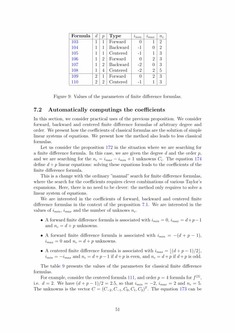
Formula d p Type imin imax nc103 1 1 Forward 0 1 2104 1 1 Backward -1 0 2105 1 1 Centered -1 1 3106 1 2 Forward 0 2 3107 1 2 Backward -2 0 3108 1 4 Centered -2 2 5109 2 1 Forward 0 2 3110 2 2 Centered -1 1 3

Figure 9: Values of the parameters of finite difference formulas.

7.2 Automatically computings the coefficients

In this section, we consider practical uses of the previous proposition. We considerforward, backward and centered finite difference formulas of arbitrary degree andorder. We present how the coefficients of classical formulas are the solution of simplelinear systems of equations. We present how the method also leads to less classicalformulas.

Let us consider the proposition 172 in the situation where we are searching fora finite difference formula. In this case, we are given the degree d and the order p,and we are searching for the nc = imax − imin + 1 unknowns Ci. The equation 174define d+ p linear equations: solving these equations leads to the coefficients of thefinite difference formula.

This is a change with the ordinary ”manual” search for finite difference formulas,where the search for the coefficients requires clever combinations of various Taylor’sexpansions. Here, there is no need to be clever: the method only requires to solve alinear system of equations.

We are interested in the coefficients of forward, backward and centered finitedifference formulas in the context of the proposition 7.1. We are interested in thevalues of imin, imax and the number of unknows nc.

• A forward finite difference formula is associated with imin = 0, imax = d+p−1and nc = d+ p unknowns.

• A forward finite difference formula is associated with imin = −(d + p − 1),imax = 0 and nc = d+ p unknowns.

• A centered finite difference formula is associated with imax = b(d+ p− 1)/2c,imin = −imax and nc = d+ p− 1 if d+ p is even, and nc = d+ p if d+ p is odd.

The table 9 presents the values of the parameters for classical finite differenceformulas.

For example, consider the centered formula 111, and order p = 4 formula for f (2),i.e. d = 2. We have (d + p − 1)/2 = 2.5, so that imin = −2, imax = 2 and nc = 5.The unknowns is the vector C = (C−2, C−1, C0, C1, C2)

T . The equation 173 can be

51

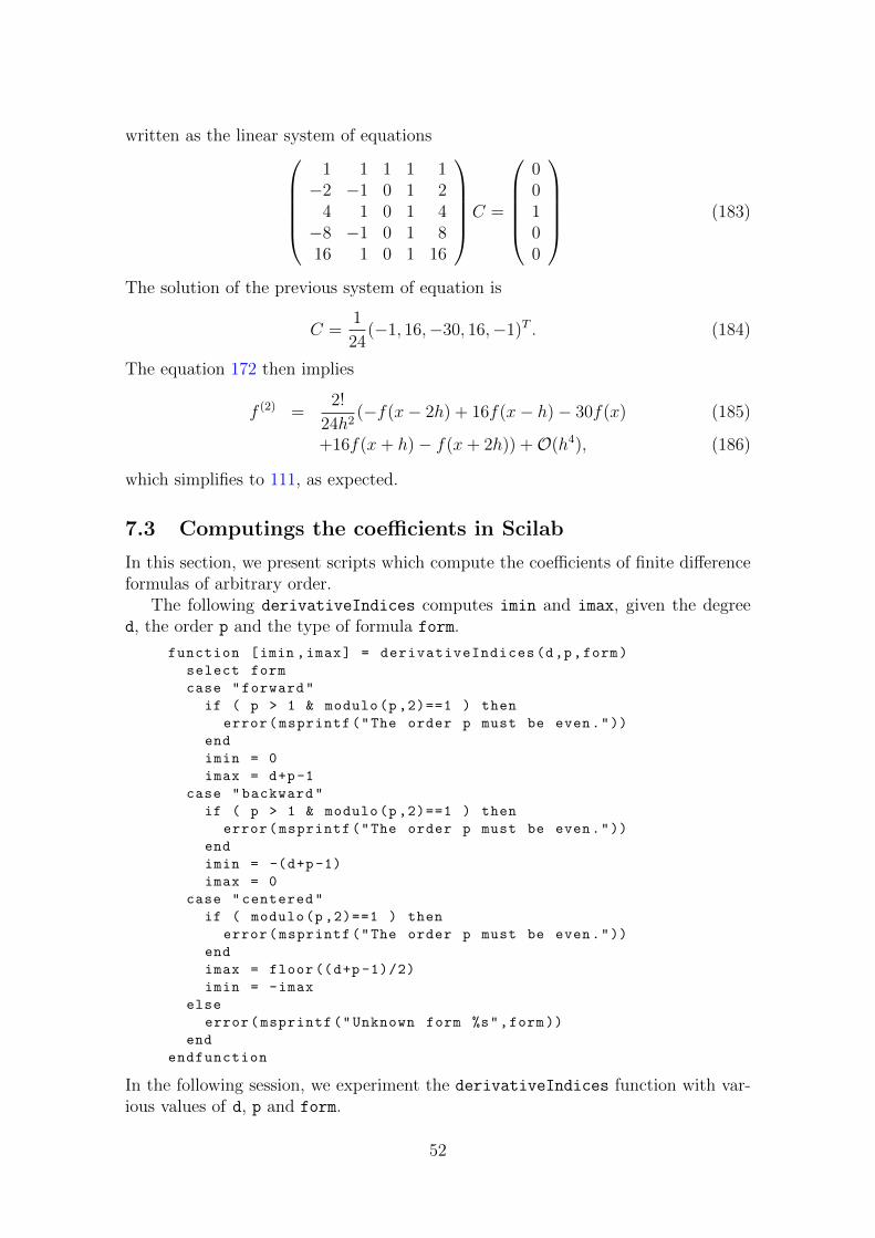
written as the linear system of equations1 1 1 1 1−2 −1 0 1 2

4 1 0 1 4−8 −1 0 1 816 1 0 1 16

C =

00100

(183)

The solution of the previous system of equation is

C =1

24(−1, 16,−30, 16,−1)T . (184)

The equation 172 then implies

f (2) =2!

24h2(−f(x− 2h) + 16f(x− h)− 30f(x) (185)

+16f(x+ h)− f(x+ 2h)) +O(h4), (186)

which simplifies to 111, as expected.

7.3 Computings the coefficients in Scilab

In this section, we present scripts which compute the coefficients of finite differenceformulas of arbitrary order.

The following derivativeIndices computes imin and imax, given the degreed, the order p and the type of formula form.

function [imin ,imax] = derivativeIndices(d,p,form)

select form

case "forward"

if ( p > 1 & modulo(p ,2)==1 ) then

error(msprintf("The order p must be even."))

end

imin = 0

imax = d+p-1

case "backward"

if ( p > 1 & modulo(p ,2)==1 ) then


end

imin = -(d+p-1)

imax = 0

case "centered"

if ( modulo(p ,2)==1 ) then


end

imax = floor((d+p -1)/2)

imin = -imax

else

error(msprintf("Unknown form %s",form))

end

endfunction

In the following session, we experiment the derivativeIndices function with var-ious values of d, p and form.

52

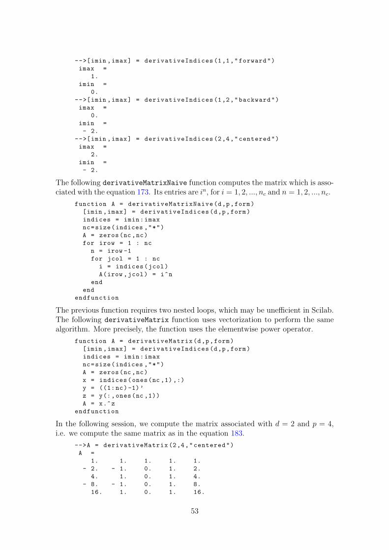
-->[imin ,imax] = derivativeIndices (1,1,"forward")

imax =

1.

imin =

0.

-->[imin ,imax] = derivativeIndices (1,2,"backward")

imax =

0.

imin =

- 2.

-->[imin ,imax] = derivativeIndices (2,4,"centered")

imax =

2.

imin =

- 2.

The following derivativeMatrixNaive function computes the matrix which is asso-ciated with the equation 173. Its entries are in, for i = 1, 2, ..., nc and n = 1, 2, ..., nc.

function A = derivativeMatrixNaive(d,p,form)

[imin ,imax] = derivativeIndices(d,p,form)

indices = imin:imax

nc=size(indices ,"*")

A = zeros(nc,nc)

for irow = 1 : nc

n = irow -1

for jcol = 1 : nc

i = indices(jcol)

A(irow ,jcol) = i^n

end

end

endfunction

The previous function requires two nested loops, which may be unefficient in Scilab.The following derivativeMatrix function uses vectorization to perform the samealgorithm. More precisely, the function uses the elementwise power operator.

function A = derivativeMatrix(d,p,form)

[imin ,imax] = derivativeIndices(d,p,form)

indices = imin:imax

nc=size(indices ,"*")

A = zeros(nc,nc)

x = indices(ones(nc ,1),:)

y = ((1:nc)-1)’

z = y(:,ones(nc ,1))

A = x.^z

endfunction

In the following session, we compute the matrix associated with d = 2 and p = 4,i.e. we compute the same matrix as in the equation 183.

-->A = derivativeMatrix (2,4,"centered")

A =

1. 1. 1. 1. 1.

- 2. - 1. 0. 1. 2.

4. 1. 0. 1. 4.

- 8. - 1. 0. 1. 8.

16. 1. 0. 1. 16.

53

d p -3 -2 -1 0 1 2 31 2 0 0 -1/2 0 1/2 0 01 4 0 1/12 -2/3 0 2/3 -1/12 01 6 -1/60 3/20 -3/4 0 3/4 -3/20 1/602 2 0 0 1 -2 1 0 02 4 0 -1/12 4/3 -5/2 4/3 -1/12 02 6 1/90 -3/20 3/2 -49/18 3/2 -3/20 1/903 2 0 -1/2 1 0 -1 1/2 03 4 1/8 -1 13/8 0 -13/8 1 -1/84 2 0 1 -4 6 -4 1 04 4 -1/6 2 -13/2 28/3 -13/2 2 -1/6

Figure 10: Coefficients of various centered finite difference formulas.

The following derivativeTemplate function solves the linear system of equations173 and computes the coefficients C.

function C = derivativeTemplate(d,p,form)

A = derivativeMatrix(d,p,form)

nc=size(A,"r")

b = zeros(nc ,1)

b(d+1) = 1

C = A\b

endfunction

In the following session, we compute the coefficients associated with d = 2 and p = 4,i.e. we compute the coefficients 184.

-->C = derivativeTemplate (2,4,"centered")

C =

- 0.0416667

0.6666667

- 1.25

0.6666667

- 0.0416667

The previous function can produce the coefficients for any degree d and order p.For example, the table 10 presents the coefficients of various centered finite differenceformulas, as presented in [22].

8 Notes and references

A reference for numerical derivatives is [1], chapter 25. ”Numerical Interpolation,Differentiation and Integration” (p. 875).

The webpage [16] and the Numerical Recipes book [14] give results about therounding errors produced by numerical derivatives.

On the specific usage of numerical derivatives in optimization, the Gill, Murrayand Wright book [8] in the section 4.6.2 ”Non-derivative Quasi-Newton methods”,

54

”Notes and Selected Bibliography for section 4.6” and the section 8.6 ”Computingfinite differences”.

The book by Nocedal and Wright [11] presents the evaluation of sparse Jaco-bians with numerical derivatives in section 7.1 ”Finite-difference derivative approxi-mations”.

The book by Kelley [12] presents in the section 2.3, ”Computing a Finite Differ-ence Jacobian” a scaling method so that the step is scaled with respect to x. Thescaling is applied only when x is large, and not when x is small. Kelley’s book [12]presents a method based on complex arithmetic is presented and is the following.

According to an article by Shampine [17], the method is due to Squire andTrapp [19]. Assume that f can be evaluated in complex arithmetic. Then Taylor’sexpansion of f shows that

f(x+ ih) = f(x) + ihf ′(x)− h2

2f ′′(x)− ih

3

6f ′′′(x) +

h4

24f ′′′′(x) + . . . (187)

We now take the imaginary part of both sides of the previous equation and dividingby h yields

Im(f(x+ ih))/h = f ′(x)− h2

6f ′′′(x) + . . . (188)

Therefore,

f ′(x) = Im(f(x+ ih))/h+O(h2). (189)

The previous formula is therefore of order 2. This method is not subject to subtrac-tive cancellation.

The Numerical Recipes [14] contains several details regarding numerical deriva-tives in chapter 5.7 ”Numerical Derivatives”. The authors present a method tocompute the step h so that the rounding error for the sum x + h is minimum.This is performed by the following algorithm, which implies a temporary variablet

t← x+ hh← t− hIn Stepleman and Winarsky’s [20] (1979), an algorithm is designed to compute

an automatic scaling for the numerical derivative. This method is an improvementof the method by Dumontet and Vignes [6] (1977). The examples tested by [6] areanalysed in [20], which shows that 11 digits are accurate with an average number offunction evaluations from 8 to 11, instead of an average 20 in [6].

In the section 7, we presented a method to compute the coefficient of finitedifference formulas. This section is based on a paper by Eberly [7], but this approachis also presented by Nicholas Maxwell in [13]. According to Maxwell, his source ofinspiration is [2], where finite difference schemes for the Laplacian are derived in asimilar way.

9 Exercises

Exercise 9.1 (Using lists with derivative) The goal of this exercise is to use lists in a practicalsituation where we want to compute the numerical derivative of a function. Consider the function

55

f : R3 → R defined by

f(x) = p1x21 + p2x

22 + p3 + p4(x3 − 1)2, (190)

where x ∈ R3 and p ∈ R4 is a given vector of parameters. In this exercise, we consider the vectorp = (4, 5, 6, 7)T . The gradient of this function is

g(x) =

2p1x1

2p2x2

2p4(x3 − 1)

. (191)

In this exercise, we want to find the minimum x? of this function with the optim function. Thefollowing script defines the function cost which allows to compute the value of this function giventhe point x and the floating point integer ind. This function returns the function value f and thegradient g.

function [f,g,ind] = cost ( x , ind )

f = 4 * x(1)^2 + 5 * x(2)^2 + 6 + 7*(x(3) -1)^2

g = [

8 * x(1)

10 * x(2)

14 * (x(3)-1)

]

endfunction

In the following session, we set the initial point and check that the function can be computed forthis initial point. Then we use the optim function and compute the optimum point xopt and thecorresponding function value fopt.

-->x0 = [1 2 3]’;

-->[f,g,ind] = cost ( x0 , 1 )

ind =

1.

g =

8.

20.

28.

f =

58.

-->[fopt ,xopt] = optim ( cost , x0 )

xopt =

- 3.677 -186

8.165 -202

1.

fopt =

6.

Use a list and find the answer to the two following questions.

1. We would like to check the gradient of the cost function. Use a list and the derivative

function to check the gradient of the function cost.

2. It would be more clear if the parameters (p1, p2, p3, p4) were explicit input arguments of thecost function. In this case, the cost function would be the following.

function [f,g,ind] = cost2 ( x , p1 , p2 , p3 , p4 , ind )

f = p1 * x(1)^2 + p2 * x(2)^2 + p3 + p4 * (x(3) -1)^2

g = [

2*p1 * x(1)

2*p2 * x(2)

2*p4 * (x(3)-1)

56

]

endfunction

Use a list and the optim function to compute the minimum of the cost2 function.

10 Acknowledgments

I would like to thank Bruno Pincon who made many highly valuable numericalcomments on this document.

References

[1] M. Abramowitz and I. A. Stegun. Handbook of Mathematical Functions withFormulas, Graphs, and Mathematical Tables. Dover Publications Inc., 1972.

[2] Laurent Anne, Quang Tran, and William Symes. Dispersion and cost analy-sis of some finite difference schemes in one-parameter acoustic wave modeling.Computational Geosciences, 1:1–33, 1997. 10.1023/A:1011576309523.

[3] Michael Baudin. Scilab is not naive. http://forge.scilab.org/index.php/

p/docscilabisnotnaive/, 2010.

[4] Michael Baudin. Floating point numbers in Scilab. http://forge.scilab.

org/index.php/p/docscifloat/, 2011.

[5] Michael Baudin. Programming in Scilab. http://forge.scilab.org/index.

php/p/docprogscilab/, 2011.

[6] J. Dumontet and J. Vignes. Determination du pas optimal dans le calcul desderivees sur ordinateur. R.A.I.R.O Analyse numerique, 11(1):13–25, 1977.

[7] David Eberly. Derivative approximation by finite differences. http://www.

geometrictools.com/Documentation/FiniteDifferences.pdf, 2008.

[8] P. E. Gill, W. Murray, and M. H. Wright. Practical optimization. AcademicPress, London, 1981.

[9] IEEE Task P754. IEEE 754-2008, Standard for Floating-Point Arithmetic.IEEE, New York, NY, USA, August 2008.

[10] P. Dugac J. Dixmier. Cours de Mathematiques du premier cycle, 1ere annee.Gauthier-Villars, 1969.

[11] Stephen J. Wright Jorge Nocedal. Numerical Optimization. Springer, 1999.

[12] C. T. Kelley. Solving nonlinear equations with Newton’s method. SIAM, 2003.

[13] Nicholas Maxwell. Notes on the derivation of finite difference kernels, on regu-larly spaced grids, using arbitrary sample points. http://people.ucalgary.

ca/~dfeder/535/FDnotes.pdf, 2010.

57

http://forge.scilab.org/index.php/p/docscilabisnotnaive/

http://forge.scilab.org/index.php/p/docscilabisnotnaive/

http://forge.scilab.org/index.php/p/docscifloat/

http://forge.scilab.org/index.php/p/docscifloat/

http://forge.scilab.org/index.php/p/docprogscilab/

http://forge.scilab.org/index.php/p/docprogscilab/

http://www.geometrictools.com/Documentation/FiniteDifferences.pdf

http://www.geometrictools.com/Documentation/FiniteDifferences.pdf

http://people.ucalgary.ca/~dfeder/535/FDnotes.pdf

http://people.ucalgary.ca/~dfeder/535/FDnotes.pdf

[14] W. H. Press, Saul A. Teukolsky, William T. Vetterling, and Brian P. Flannery.Numerical Recipes in C, Second Edition. Cambridge University Press, 1992.

[15] Wolfram Research. Wolfram alpha. http://www.wolframalpha.com.

[16] K.E. Schmidt. Numerical derivatives. http://fermi.la.asu.edu/PHY531/

intro/node1.html.

[17] L. F. Shampine. Accurate numerical derivatives in Matlab. ACM Trans. Math.Softw., 33(4):26, 2007.

[18] Amit Soni and Alan Edelman. An Analysis of Scientific Computing Environ-ments: A Consumer’s View. June 2008.

[19] William Squire and George Trapp. Using complex variables to estimate deriva-tives of real functions. SIAM Rev., 40(1):110–112, 1998.

[20] R. S. Stepleman and N. D. Winarsky. Adaptive numerical differentiation. Math-ematics of Computation, 33(148):1257–1264, 1979.

[21] David Stevenson. IEEE standard for binary floating-point arithmetic, August1985.

[22] Wikipedia. Finite difference coefficient — wikipedia, the free encyclopedia,2011. [Online; accessed 13-October-2011].

58

http://www.wolframalpha.com

http://fermi.la.asu.edu/PHY531/intro/node1.html

http://fermi.la.asu.edu/PHY531/intro/node1.html

Index

derivative, 6numdiff, 46

Centered (2 points) finite difference forf ′, 17

Centered (3 points) finite difference forf ′′, 22

Centered (4 points) finite difference forf ′, 19

Forward (2 points) finite difference for f ′,5

gradient, 27

Jacobian, 28

order, 5

Taylor formula, 4Truncation error, 5

59

Numerical Derivatives in Scilab - forge.scilab.org · Numerical Derivatives in Scilab Micha el...

Documents

Transcript of Numerical Derivatives in Scilab - forge.scilab.org · Numerical Derivatives in Scilab Micha el...