improved numerical techniques for occupation-time derivatives and
251
IMPROVED NUMERICAL TECHNIQUES FOR OCCUPATION-TIME DERIVATIVES AND OTHER COMPLEX FINANCIAL INSTRUMENTS Johnson, Paul 2008 MIMS EPrint: 2009.92 Manchester Institute for Mathematical Sciences School of Mathematics The University of Manchester Reports available from: http://eprints.maths.manchester.ac.uk/ And by contacting: The MIMS Secretary School of Mathematics The University of Manchester Manchester, M13 9PL, UK ISSN 1749-9097
Transcript of improved numerical techniques for occupation-time derivatives and

IMPROVED NUMERICAL TECHNIQUES FOROCCUPATION-TIME DERIVATIVES AND
OTHER COMPLEX FINANCIALINSTRUMENTS
Johnson, Paul
2008
MIMS EPrint: 2009.92
Manchester Institute for Mathematical SciencesSchool of Mathematics
The University of Manchester
Reports available from: http://eprints.maths.manchester.ac.uk/And by contacting: The MIMS Secretary
School of Mathematics
The University of Manchester
Manchester, M13 9PL, UK
ISSN 1749-9097
IMPROVED NUMERICAL
TECHNIQUES FOR
OCCUPATION-TIME DERIVATIVES
AND OTHER COMPLEX FINANCIAL
INSTRUMENTS
A thesis submitted to the University of Manchester
for the degree of Doctor of Philosophy
in the Faculty of Engineering and Physical Sciences
2008
Paul Johnson
School of Mathematics

Contents
Abstract 11
Declaration 12
Copyright 13
Acknowledgements 14
1 Introduction 15
1.1 Background . . . . . . . . . . . . . . . . . . . . . . . . . . . . . . . . 15
1.2 Options . . . . . . . . . . . . . . . . . . . . . . . . . . . . . . . . . . 16
1.2.1 Arbitrage-free Pricing . . . . . . . . . . . . . . . . . . . . . . 17
1.2.2 The Black, Scholes and Merton Framework . . . . . . . . . . . 17
1.2.3 The Black-Scholes Equation . . . . . . . . . . . . . . . . . . . 18
1.3 Numerical Techniques . . . . . . . . . . . . . . . . . . . . . . . . . . 18
1.3.1 Monte-Carlo methods . . . . . . . . . . . . . . . . . . . . . . . 19
1.3.2 Lattice Methods . . . . . . . . . . . . . . . . . . . . . . . . . . 21
1.3.3 Finite-Difference Methods . . . . . . . . . . . . . . . . . . . . 25
1.3.4 Richardson Extrapolation . . . . . . . . . . . . . . . . . . . . 30
1.3.5 Overview . . . . . . . . . . . . . . . . . . . . . . . . . . . . . 30
2 Advanced Numerical Techniques 32
2.1 Introduction . . . . . . . . . . . . . . . . . . . . . . . . . . . . . . . . 32
2.2 Formulation . . . . . . . . . . . . . . . . . . . . . . . . . . . . . . . . 35
2.3 Asymptotic analysis of the American option near expiry . . . . . . . 38
2

2.3.1 The American call with 0 < d < r . . . . . . . . . . . . . . . . 39
2.3.2 Asymptotic analysis for the case d ≥ r . . . . . . . . . . . . . 42
2.3.3 The American put with dividends . . . . . . . . . . . . . . . . 48
2.4 Numerical Techniques and extensions . . . . . . . . . . . . . . . . . . 48
2.4.1 The PSOR Method . . . . . . . . . . . . . . . . . . . . . . . . 49
2.4.2 Modifying PSOR - A Novel Approach . . . . . . . . . . . . . . 52
2.4.3 The Boundary-fitted Coordinate Formulation . . . . . . . . . 55
2.5 An Improved Numerical Technique . . . . . . . . . . . . . . . . . . . 57
2.5.1 The Advanced Body-Fitted Coordinated Method (ABFC) . . 60
2.6 Results . . . . . . . . . . . . . . . . . . . . . . . . . . . . . . . . . . . 61
2.7 Conclusions . . . . . . . . . . . . . . . . . . . . . . . . . . . . . . . . 66
3 Multi-Asset American Options 68
3.1 Literature . . . . . . . . . . . . . . . . . . . . . . . . . . . . . . . . . 70
3.2 The Multi-Asset BSM Equation . . . . . . . . . . . . . . . . . . . . . 74
3.2.1 Maximum Options . . . . . . . . . . . . . . . . . . . . . . . . 76
3.3 Numerical methods for the European Option . . . . . . . . . . . . . . 82
3.3.1 Results . . . . . . . . . . . . . . . . . . . . . . . . . . . . . . . 85
3.4 American Options . . . . . . . . . . . . . . . . . . . . . . . . . . . . . 87
3.4.1 Multi-Asset American Option . . . . . . . . . . . . . . . . . . 89
3.4.2 PSOR on Multi-Asset Options . . . . . . . . . . . . . . . . . . 92
3.5 Results . . . . . . . . . . . . . . . . . . . . . . . . . . . . . . . . . . . 93
3.5.1 The Early Exercise Region . . . . . . . . . . . . . . . . . . . . 93
3.6 Enhanced Numerical Techniques . . . . . . . . . . . . . . . . . . . . . 98
3.6.1 Optimising the relaxation parameter ω . . . . . . . . . . . . . 98
3.6.2 Simple Banding . . . . . . . . . . . . . . . . . . . . . . . . . . 98
3.6.3 Boundary Updating Solver . . . . . . . . . . . . . . . . . . . . 104
3.6.4 Comparison of methods . . . . . . . . . . . . . . . . . . . . . 106
3.7 Conclusions . . . . . . . . . . . . . . . . . . . . . . . . . . . . . . . . 108
3

4 Time Dependent Barrier Options 109
4.1 Occupation-Time Derivatives . . . . . . . . . . . . . . . . . . . . . . 110
4.2 Parisian Options . . . . . . . . . . . . . . . . . . . . . . . . . . . . . 114
4.2.1 Parisian Options – Boundary Conditions . . . . . . . . . . . . 115
4.2.2 Numerical Method . . . . . . . . . . . . . . . . . . . . . . . . 117
4.2.3 Two Numerical Schemes . . . . . . . . . . . . . . . . . . . . . 118
4.2.4 Implementing the Schemes on a Parisian Option . . . . . . . . 120
4.3 ParAsian Options . . . . . . . . . . . . . . . . . . . . . . . . . . . . . 121
4.3.1 ParAsian Options – Boundary Conditions . . . . . . . . . . . 122
4.3.2 Implementing the schemes on a ParAsian Option . . . . . . . 122
4.4 Results . . . . . . . . . . . . . . . . . . . . . . . . . . . . . . . . . . . 123
4.4.1 Parisian Options . . . . . . . . . . . . . . . . . . . . . . . . . 126
4.4.2 ParAsian Options . . . . . . . . . . . . . . . . . . . . . . . . . 129
4.5 A New Option – The Integral Time Model . . . . . . . . . . . . . . . 130
4.5.1 Implementing a Crank-Nicolson Scheme on the IT option . . . 132
4.5.2 An implicit scheme for the IT option . . . . . . . . . . . . . . 135
4.5.3 Results – ParAsian IT Options . . . . . . . . . . . . . . . . . 135
4.6 Conclusions . . . . . . . . . . . . . . . . . . . . . . . . . . . . . . . . 137
5 Modelling Bankruptcy with ParAsian Options 138
5.1 Literature . . . . . . . . . . . . . . . . . . . . . . . . . . . . . . . . . 139
5.2 The Model . . . . . . . . . . . . . . . . . . . . . . . . . . . . . . . . . 141
5.3 The Valuation Framework . . . . . . . . . . . . . . . . . . . . . . . . 143
5.3.1 Assumptions . . . . . . . . . . . . . . . . . . . . . . . . . . . . 143
5.3.2 Partial differential equation - derivation . . . . . . . . . . . . . 147
5.3.3 Boundary conditions . . . . . . . . . . . . . . . . . . . . . . . 147
5.3.4 Parameter choices . . . . . . . . . . . . . . . . . . . . . . . . . 150
5.4 Numerical Method . . . . . . . . . . . . . . . . . . . . . . . . . . . . 151
5.5 Results for a Single Class of Debt . . . . . . . . . . . . . . . . . . . . 155
5.5.1 Credit Spread and Firm Rating . . . . . . . . . . . . . . . . . 155
4

5.5.2 Credit Spread and Window length T . . . . . . . . . . . . . . 156
5.5.3 Interest rate and debt accumulation factor . . . . . . . . . . . 157
5.5.4 Duration . . . . . . . . . . . . . . . . . . . . . . . . . . . . . . 160
5.6 Results for a Two-Class Debt Structure . . . . . . . . . . . . . . . . . 161
5.6.1 Credit spread and priority . . . . . . . . . . . . . . . . . . . . 161
5.6.2 Credit spread and interest rate volatility . . . . . . . . . . . . 165
5.6.3 Credit spread and default barrier . . . . . . . . . . . . . . . . 166
5.6.4 Credit spread and window length . . . . . . . . . . . . . . . . 169
5.7 Conclusions . . . . . . . . . . . . . . . . . . . . . . . . . . . . . . . . 172
6 Convertible Bonds 174
6.1 Literature . . . . . . . . . . . . . . . . . . . . . . . . . . . . . . . . . 175
6.2 The Model . . . . . . . . . . . . . . . . . . . . . . . . . . . . . . . . . 180
6.2.1 The Governing PDE . . . . . . . . . . . . . . . . . . . . . . . 181
6.2.2 At Maturity . . . . . . . . . . . . . . . . . . . . . . . . . . . . 182
6.2.3 Default Barrier . . . . . . . . . . . . . . . . . . . . . . . . . . 183
6.2.4 Optimal Call and Conversion . . . . . . . . . . . . . . . . . . 184
6.3 Numerical methods . . . . . . . . . . . . . . . . . . . . . . . . . . . . 185
6.4 Results . . . . . . . . . . . . . . . . . . . . . . . . . . . . . . . . . . . 187
6.5 Conclusions . . . . . . . . . . . . . . . . . . . . . . . . . . . . . . . . 195
7 A New Class of Option 197
7.1 The American Option as a Barrier Option . . . . . . . . . . . . . . . 198
7.2 The Delayed-Exercise Option . . . . . . . . . . . . . . . . . . . . . . 199
7.2.1 Rational Pricing . . . . . . . . . . . . . . . . . . . . . . . . . 201
7.2.2 Pricing the delayed-exercise option . . . . . . . . . . . . . . . 203
7.2.3 The Existence of the Implied Barrier . . . . . . . . . . . . . . 205
7.3 Numerical Analysis . . . . . . . . . . . . . . . . . . . . . . . . . . . . 207
7.3.1 The Delayed-Exercise Option Algorithm . . . . . . . . . . . . 209
7.4 Results . . . . . . . . . . . . . . . . . . . . . . . . . . . . . . . . . . . 210
7.5 The Perpetual Case . . . . . . . . . . . . . . . . . . . . . . . . . . . . 217
5
7.5.1 Asymptotic analysis – in the limit as time-to-knockout tends
to zero . . . . . . . . . . . . . . . . . . . . . . . . . . . . . . . 219
7.5.2 Solution to the ODE . . . . . . . . . . . . . . . . . . . . . . . 222
7.6 Advanced Body-Fitted Solver for the Delayed-Exercise Option . . . . 224
7.7 Conclusions . . . . . . . . . . . . . . . . . . . . . . . . . . . . . . . . 231
8 Conclusions 232
A Numerical Schemes 234
A.1 BFC and ABFC coefficients . . . . . . . . . . . . . . . . . . . . . . . 234
References 237
Word count 65316
6

List of Tables
2.1 Relative RMS errors for American Put Options . . . . . . . . . . . . 63
2.2 Relative RMS and ABS errors for American Call Options . . . . . . . 65
3.1 Relative RMS errors for European dual strike put options . . . . . . . 88
3.2 Relative RMS errors for American dual strike put options . . . . . . . 107
4.1 Convergence of the Parisian solver . . . . . . . . . . . . . . . . . . . . 127
4.2 Comparison of results . . . . . . . . . . . . . . . . . . . . . . . . . . . 128
5.1 Leverage Ratio and Asset Volatility For Each Rating . . . . . . . . . 151
5.2 Convergence of the bond price . . . . . . . . . . . . . . . . . . . . . . 155
6.1 Convergence of the convertible bond price . . . . . . . . . . . . . . . 186
6.2 Parameters . . . . . . . . . . . . . . . . . . . . . . . . . . . . . . . . 187
7.1 Relative RMS errors for delayed-exercise put options . . . . . . . . . 229
7
List of Figures
1.1 Stock and option value in a three-step binomial tree. . . . . . . . . . 22
2.1 The European put option. . . . . . . . . . . . . . . . . . . . . . . . . 36
2.2 The American put option. . . . . . . . . . . . . . . . . . . . . . . . . 37
2.3 The simple structure for an American call with 0 < d < r. . . . . . . 42
2.4 The simple structure for an American call with d ≥ r. . . . . . . . . . 47
2.5 Advanced PSOR solver – pseudo code . . . . . . . . . . . . . . . . . . 54
2.6 Point Solver Down – pseudo code . . . . . . . . . . . . . . . . . . . . 54
2.7 Convergence . . . . . . . . . . . . . . . . . . . . . . . . . . . . . . . . 62
2.8 Convergence for different time steps . . . . . . . . . . . . . . . . . . . 64
2.9 The free boundary - BFC vs. PSOR vs. ABFC . . . . . . . . . . . . 66
3.1 The minimum of two vanilla options. . . . . . . . . . . . . . . . . . . 85
3.2 The maximum of two vanilla options . . . . . . . . . . . . . . . . . . 86
3.3 The 2-asset correlation option. . . . . . . . . . . . . . . . . . . . . . . 86
3.4 The portfolio option. . . . . . . . . . . . . . . . . . . . . . . . . . . . 86
3.5 The early exercise regions for the maximum of two puts option. . . . 90
3.6 American single strike option . . . . . . . . . . . . . . . . . . . . . . 95
3.7 American portfolio option . . . . . . . . . . . . . . . . . . . . . . . . 96
3.8 American dual strike option . . . . . . . . . . . . . . . . . . . . . . . 97
3.9 Simple banded estimate . . . . . . . . . . . . . . . . . . . . . . . . . 104
3.10 Point solver down – pseudo code . . . . . . . . . . . . . . . . . . . . . 105
3.11 PointSolverUp – pseudo code . . . . . . . . . . . . . . . . . . . . . . 105
3.12 The advanced PSOR algorithm – pseudo code . . . . . . . . . . . . . 106
8

4.1 Parisian up-and-out option vs. time-to-knockout close to maturity . . 124
4.2 Parisian up-and-out option value vs. time-to-knockout. . . . . . . . . 125
4.3 Parisian option value/delta vs. asset price and time-to-knockout . . . 127
4.4 ParAsian option value/delta vs. asset price and time-to-knockout . . 129
4.5 Parisian/ParAsian option value/delta vs. asset price. . . . . . . . . . 130
4.6 A Monte-Carlo simulation of how the area over the barrier is formed. 132
4.8 ParAsian integral time option value/delta vs. asset price and time-to-
knockout. . . . . . . . . . . . . . . . . . . . . . . . . . . . . . . . . . 135
4.9 The value of the ParAsian integral time option gamma and the ParAsian
option gamma. . . . . . . . . . . . . . . . . . . . . . . . . . . . . . . 136
5.1 Payoffs to Junior and Senior Debt Issues When Junior Debt Matures
First. . . . . . . . . . . . . . . . . . . . . . . . . . . . . . . . . . . . . 143
5.2 Term Structure of Credit Spreads. . . . . . . . . . . . . . . . . . . . . 156
5.3 Term Structure of Credit Spreads and Window Length . . . . . . . . 157
5.4 Credit Spread vs. Window Length . . . . . . . . . . . . . . . . . . . . 158
5.5 Term structure for varying interest rate in a one-factor model . . . . 158
5.6 Term structure for varying stochastic interest rate, single issue debt . 159
5.7 Duration . . . . . . . . . . . . . . . . . . . . . . . . . . . . . . . . . . 161
5.8 Senior Debt Matures First. . . . . . . . . . . . . . . . . . . . . . . . . 162
5.9 Senior Debt Matures Second . . . . . . . . . . . . . . . . . . . . . . . 164
5.10 Credit Spread vs. Volatility of Interest Rate . . . . . . . . . . . . . . 165
5.11 Credit Spread vs. Default Barrier Level, with Senior Debt Maturing
First . . . . . . . . . . . . . . . . . . . . . . . . . . . . . . . . . . . . 166
5.12 Credit Spread vs. Default Barrier Level, with Senior Debt Maturing
Second . . . . . . . . . . . . . . . . . . . . . . . . . . . . . . . . . . . 168
5.13 Credit Spread vs. Window Length, with Senior Debt Maturing First . 170
5.14 Credit Spread vs. Window Length, with Senior Debt Maturing Second 171
6.1 Convertible bond value for different ratings . . . . . . . . . . . . . . . 188
6.2 Optimum conversion price for different ratings . . . . . . . . . . . . . 189
9

6.3 Convertible bond price against volatility. . . . . . . . . . . . . . . . . 192
6.4 Convertible bond price against long term interest rate. . . . . . . . . 192
6.5 Capital structure of the firm’s debt . . . . . . . . . . . . . . . . . . . 193
6.6 Convertible bond with call option. . . . . . . . . . . . . . . . . . . . . 195
7.1 Monte Carlo simulation. . . . . . . . . . . . . . . . . . . . . . . . . . 204
7.2 Grid search algorithm – pseudo code . . . . . . . . . . . . . . . . . . 209
7.3 The delayed-exercise put option . . . . . . . . . . . . . . . . . . . . . 210
7.4 The exercise premium. . . . . . . . . . . . . . . . . . . . . . . . . . . 211
7.5 The delay option. . . . . . . . . . . . . . . . . . . . . . . . . . . . . . 212
7.6 Barrier H vs. time to knockout and root time to knockout. . . . . . . 213
7.7 Barrier H vs. time to maturity and log time. . . . . . . . . . . . . . . 214
7.8 Barrier H vs time to maturity and log time . . . . . . . . . . . . . . 214
7.9 The Greeks. . . . . . . . . . . . . . . . . . . . . . . . . . . . . . . . . 215
7.10 The Greeks, zoomed region. . . . . . . . . . . . . . . . . . . . . . . . 216
7.11 The value of θ = ∂V/∂τ . . . . . . . . . . . . . . . . . . . . . . . . . 217
7.12 Asymptotic approximation to the perpetual case . . . . . . . . . . . . 224
7.13 Asymptotic H(τ, τ ) vs. time to knockout . . . . . . . . . . . . . . . 230
7.14 Free boundary approximation S∗f(τ) vs. time to maturity . . . . . . . 230
10

Abstract
Occupation-time derivatives are complex barrier-type options where valuation
depends on the time spent beyond the barrier by the underlying asset. This the-
sis presents a model for corporate bonds using an occupation-time derivative, the
ParAsian option, the features of which can capture bankruptcy resolution and com-
plex capital structure with violations of the absolute priority rule. It investigates the
numerics of the problem, and proposes appropriate numerical techniques to enable
accurate and rapid solutions. The model is extended to include bond conversion in
a two-tier structure, which presents its own numerical problems. A new occupation-
time derivative that takes into account the distance of deviations beyond the barrier
is presented and solved.
Using existing knowledge on the asymptotic structure, new fast and efficient tech-
niques are created for pricing American options. A second new occupation-time
derivative is proposed, combining elements of early exercise with the ParAsian op-
tion to produce the American delayed-exercise option.
The numerical methods employed in this thesis are based on accurate finite-
difference schemes, specifically developed and enhanced to treat the various classes
of problem considered.
11

Declaration
No portion of the work referred to in this thesis has been
submitted in support of an application for another degree
or qualification of this or any other university or other
institute of learning.
12

Copyright
Copyright in text of this thesis rests with the author. Copies (by any process)
either in full, or of extracts, may be made only in accordance with instructions given
by the author and lodged in the John Rylands University Library of Manchester.
Details may be obtained from the Librarian. This page must form part of any such
copies made. Further copies (by any process) of copies made in accordance with such
instructions may not be made without the permission (in writing) of the author.
The ownership of any intellectual property rights which may be described in this
thesis is vested in The University of Manchester, subject to any prior agreement to
the contrary, and may not be made available for use by third parties without the
written permission of the University, which will prescribe the terms and conditions
of any such agreement.
Further information on the conditions under which disclosures and exploitation
may take place is available from the Head of the School of Mathematics.
13

Acknowledgements
Many thanks to my supervisors Peter Duck and David Newton who have given
guidance and support throughout the PhD, especially when I fell ill for some time.
Their thoughts and comments are always well appreciated, and always available.
I would like to thank my Mum. Special mentions go to my girlfriend Helen for
her love and support and my sister Anna, who has provided me with free board and
lodge at various stages of the PhD. Thanks also to Nick Sharp and Lingzhi Yu for
useful discussions on the work presented in this Thesis.
14

Chapter 1
Introduction
1.1 Background
A derivative is a financial contract, whose value depends on some underlying
asset. Even though derivatives had existed for some time, it was not until the early
1970’s that derivative markets became fully established. Around the same time as
the papers of Black and Scholes (1973) and Merton (1973) set a framework in which
simple European options could be priced, the Chicago Board of Options Exchange
was formed to trade OTC (over the counter) options. The trading in options has
been increasing ever since with no sign of abating; recent growth shows the OTC
derivatives market increase from 220 trillion in the first half of 2004 to 370 trillion in
the first half of 20061.
The Black, Scholes and Merton model (BSM) is still the benchmark, and, al-
though it is by no means perfect, the fundamental assumptions of no arbitrage and
random walk will be hard to shake off for some time yet. From this model, we arrive
at the celebrated Black-Scholes partial differential equation (PDE), which has excited
mathematicians and physicists almost as much as it has the finance world. Driven
by the markets, the need for ever more complex financial derivatives has led to inter-
esting mathematical problems, many of which do not have closed form or analytical
1The notional amount outstanding taken from the regular OTC derivatives market statistics 17thNovember 2006. http://www.bis.org
15

CHAPTER 1. INTRODUCTION 16
solutions.
In this thesis we concentrate mainly on exotic options, for which there are no
known closed form or analytical solutions. Early work in collaboration with Lingzhi
Yu, in Yu (2004), developed a model for corporate bonds, where the corporate bond
is seen as a contingent claim on a firm. In addition, new methods are proposed for
solving the numerical problems involved in pricing such an option. The numerical
methods must tackle multiple dimensions, barriers and early exercise when the bond
is convertible. Along the way we also propose two new classes of barrier option, both
extensions to current occupational time derivatives.
1.2 Options
First, let us introduce the concept of an option. In its simplest form, the holder
of an option has the right to buy (with a call option) or sell (with a put option) the
underlying asset for a given price at or before some maturity date. The asset may be
traded, such as stock, currency, commodity, but also can be something measurable
such as temperature, or the volatility of a stock; or even another derivative. With
an option, the writer of the option (who sells it to another party), takes on all of
the risk and as compensation, the holder must pay a premium for this. The insight
impounded by the BSM framework was that the writer of the option can eliminate
risk by replicating the option using a self-financing dynamic hedging strategy with
an underlying asset and the option, one side bought, one side sold, so as to produce
a portfolio that is locally riskless. If it is possible to construct such a portfolio in
the market, then the market is said to be complete. An option on temperature is a
classic example of incomplete markets, as the underlying asset, temperature, cannot
be bought or sold. Therefore we cannot hedge the option and as a consequence the
option is priced as the expected discounted value.

CHAPTER 1. INTRODUCTION 17
1.2.1 Arbitrage-free Pricing
When pricing derivatives one of the fundamental assumptions is that of arbi-
trage. Arbitrage is the practice of taking advantage of an opportunity presented by
market prices to make an instantaneous profit. In the Black-Scholes framework we
assume that the option prices reflect an arbitrage-free market, in that any mispricing
will be ‘arbitraged’ away.
1.2.2 The Black, Scholes and Merton Framework
The BSM analysis starts by assuming that the asset price S follows a lognormal
geometric Brownian motion process
dS
S= (µ− d)dt+ σdWt, (1.1)
where µ, d and σ are constants, which represent the expected return, the continuous
dividend rate and the volatility of the asset respectively. The process W is a Wiener
process, capturing the uncertainty in the market. Equation (1.1) is the stochastic
differential equation (SDE) for the asset price. In this thesis, we will assume that the
asset price always follows that process. There is evidence to suggest that this is not
strictly followed by stock prices: the distribution of returns exhibits sharper peaks and
fatter tails than would be expected from the model. Notable attempts to address this
problem are to include a jump process (Merton, 1976), stochastic volatility (Heston,
1993), and the local volatility model (Dupire, 1994). These solutions however, come
with their own problems, and we are not yet at the stage where the lognormal process
must be abandoned. Moreover, deviations from Brownian motion only become more
significant under certain conditions, most especially longer time to maturity of an
option, or for certain underlyings, such as oil prices or interest rates (in the long
term). For the mass of options traded with maturities under a year, Brownian motion
can remain a practical modelling assumption.
As well as the assumption of an arbitrage-free market, trading in the asset must

CHAPTER 1. INTRODUCTION 18
be unrestricted, i.e. no transaction costs, continuous trading and shortselling allowed,
and assets are divisible. An investor may also invest at a risk-free rate r, which is
commonly taken to be constant over time.
1.2.3 The Black-Scholes Equation
Assuming that a derivative V is a function of S and t, and is twice differentiable,
then we may apply Ito’s lemma to show that
dV =
(
∂V
∂t+ (µ− d)S∂V
∂S+
1
2σ2S2∂
2V
∂S2
)
dt+ σS∂V
∂SdW. (1.2)
Then by setting up a risk-free portfolio such that,
Π = V (S, t)− ∂V
∂SS (1.3)
we have that
dΠ =
(
∂V
∂t+
1
2σ2S2∂
2V
∂S2
)
dt. (1.4)
The return on this portfolio is locally riskless. Because we could have invested the ini-
tial capital risklessly, to ensure the arbitrage-free market, the return on the portfolio
must be equal to the risk-free rate. So then, the derivative’s price must satisfy
∂V
∂t+
1
2σ2S2∂
2V
∂S2+ (r − d)S∂V
∂S− rV = 0. (1.5)
This is the Black-Scholes equation. It is the fundamental equation for derivative
pricing.
1.3 Numerical Techniques
In this section we give a brief overview of the numerical techniques commonly
used to solve for different options.

CHAPTER 1. INTRODUCTION 19
1.3.1 Monte-Carlo methods
The Monte-Carlo method is the simplest of all approaches. As first suggested by
Boyle (1977), the price is derived by simulating a large number of the random sample
paths under the risk-neutral measure, calculating the value of said paths, and then
discounting back and taking the average.
Let the process followed by the underlying asset value in a risk-neutral world be
dS = µSdt+ σSdW (1.6)
where dW is a Weiner process, σ is the volatility and µ is the rate of return in
a risk-neutral world. We can approximate (1.6) with greater accuracy if we non-
dimensionalize the problem to be in terms of lnS. From Ito’s lemma we can write
the process followed by lnS as
d lnS =(
µ− 12σ2)
dt+ σdW. (1.7)
Then to simulate paths, we can write (1.7) as
δ lnS =(
µ− 12σ2)
δt+ σφ√δt,
where φ is a random sample drawn from the normal distribution and δt may be any
size required.
If S is a non-dividend paying stock then we may replace µ by r, the risk-free
interest rate. Consequently the value of the stock at time t+ δt is
S(t+ δt) = S(t) exp{
(
r − 12σ2)
δt+ σφ√δt}
. (1.8)
The value of the asset can be calculated at however many points in time are needed
to calculate the value of the option. For a simple European option the only time we
need to know the value of the asset is at maturity. The value of a vanilla European

CHAPTER 1. INTRODUCTION 20
call option with n sample paths can be expressed as
V (S0, t = 0) =1
n
n∑
i=1
e−rT max[
S0 exp{
(
r − 12σ2)
T + σφi
√T}
− E, 0]
. (1.9)
More complex options will require the calculation of the asset value at multiple times.
In terms of errors for a calculation such as (1.9), from simple statistics the standard
error of the estimate is
ω√N
where ω is the standard deviation of the results. Then if µ is the mean price, we can
construct a confidence interval so that the exact value Ve is given by
µ− ψ ω√N< Ve < µ+ ψ
ω√N,
where ψ determines the percentage confidence. Then in order to reduce the errors by
a factor of 2, we must quadruple the number of trials.
The main advantage of the approach is the ability to extend it to multiple dimen-
sions with only a linear extension in calculations. The convergence of the method as
shown above is O(1/√n) for a European option, and is independent of the number
of dimensions. In terms of work done to generate a solution, the linear increase in
calculations allied with O(1/√n) convergence makes the Monte-Carlo method com-
parable to the binomial method (see below) where calculations increase by a power
of 2 and the convergence is O(1/n). The forward path simulation makes solving
for complicated path-dependent options simple, although optimal strategies can be
harder to generate. The Monte-Carlo method also has a distinct advantage that the
stochastic process may be arbitrary – even collected data may be used as input. The
literature focuses on methods to improve the convergence of the method by reducing
bias and variance, the pricing of derivatives with American features and also SDEs
with nonlinear components.
In order to price American features, one must generate the optimal exercise strat-
egy for the option. Perhaps the simplest method to understand is the regression-based
CHAPTER 1. INTRODUCTION 21
approach of Longstaff and Schwartz (2001). The crux of the method is to identify the
conditional expected value of continuation. After generating a set of asset paths over
a number of time steps, the method works backward from expiry. We generate the
value of the ‘option to continue’ at the current time step for all possible asset values
by using least-squares regression analysis on all the discounted future payments for
each path. Then comparing the value of exercising at that point with the value of
continuing to the next time step we can choose the optimal path.
1.3.2 Lattice Methods
A lattice method can be considered as a discrete time model of the varying price
over time of the underlying asset. The first lattice method was the binomial model
proposed by Cox et al. (1979). The trinomial model was studied by Parkinson (1977)
and then again by Boyle (1986). The basic idea is the same for both methods, so we
will just discuss the binomial method.
The binomial model uses a discrete-time framework, where the duration of the
option from the start to expiry is divided into n time steps of equal length, δt.
Starting with an asset price S at time t = 0, at the next period of time the asset
price can either move up to Su, with probability p, or have moved down to Sd, with
probability (1− p), where u > 1 and d < 1 are independent of the asset price. On a
lattice, the position of the asset price at a particular time is described as a node.
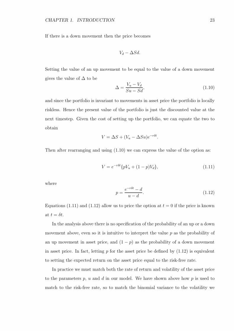
In figure 1.1 a three step binomial tree is shown. In order to price an option, we
will price a portfolio containing a long position in the option and short a quantity ∆
in the asset. Then by arbitrage, we may calculate the value of ∆ which forces the
portfolio to be riskless. Take for instance the first step in figure 1.1, the value of the
portfolio is initially V −∆S, and if there is an up movement in the stock price the
value becomes
Vu −∆Su.

CHAPTER 1. INTRODUCTION 22
S
V
Su
Vu
Sd
Vd
Su2
Vuu
Sud
Vud
Sd2
Vdd
Su3
Vuuu
Su2d
Vuud
Sud2
Vudd
Sd3
Vddd
Figure 1.1Stock and option value in a three-step binomial tree.
CHAPTER 1. INTRODUCTION 23
If there is a down movement then the price becomes
Vd −∆Sd.
Setting the value of an up movement to be equal to the value of a down movement
gives the value of ∆ to be
∆ =Vu − Vd
Su− Sd, (1.10)
and since the portfolio is invariant to movements in asset price the portfolio is locally
riskless. Hence the present value of the portfolio is just the discounted value at the
next timestep. Given the cost of setting up the portfolio, we can equate the two to
obtain
V = ∆S + (Vu −∆Su)e−rδt.
Then after rearranging and using (1.10) we can express the value of the option as:
V = e−rδt{pVu + (1− p)Vd}, (1.11)
where
p =e−rδt − du− d . (1.12)
Equations (1.11) and (1.12) allow us to price the option at t = 0 if the price is known
at t = δt.
In the analysis above there is no specification of the probability of an up or a down
movement above, even so it is intuitive to interpret the value p as the probability of
an up movement in asset price, and (1 − p) as the probability of a down movement
in asset price. In fact, letting p for the asset price be defined by (1.12) is equivalent
to setting the expected return on the asset price equal to the risk-free rate.
In practice we must match both the rate of return and volatility of the asset price
to the parameters p, u and d in our model. We have shown above how p is used to
match to the risk-free rate, so to match the binomial variance to the volatility we

CHAPTER 1. INTRODUCTION 24
have
pu2 + (1− p)d2 − (pu+ (1− p)d)2 = σ2δt, (1.13)
and we have two equations in three unknowns, so there still exists a degree of freedom.
This freedom allows for different parameter choices, which could be tailored to the
problem. A simple choice is that of Cox et al. (1979), who set
ud = 1. (1.14)
so that the distance moved up is the same as the distance moved down for the
lognormal walk. After some algebra we find that u = eσδt and d = e−σδt. Another
popular choice is that of Amin (1991), who choose u and d so that p = 12
and there
is an equal chance of moving up or down.
In order to price an option using the full binomial tree, we must start at expiry, at
which point we know the value of the option. Then for all nodes at T − δt, the value
is given by (1.11). Then by working recursively through the tree we will eventually
reach t = 0 and hence the value of the option at t = 0.
Applications and convergence
Lattice methods are easily applied to European, American (Bermudan) options.
For the European option, the convergence is 1/n for binomial tree calculation, un-
modified, as described above. However misplacing of nodes at expiry can lead to large
errors. This has been addressed in the literature (Widdicks et al., 2002) and with
careful Richardson extrapolation the rate of convergence can be improved to 1/n2.
Although the extension from European to Bermudan and American is simple to
code, the reduction of the errors are not quite so simple here. As well as the errors at
expiry due to the exercise price, the position of the free boundary at each time step
also introduces some form of error. This means that the techniques introduced for
the European option, although effective in increasing accuracy, cannot improve the
convergence rate above 1/n (Broadie and Detemple, 1996; Figlewski and Gao, 1999;
Leisen, 1998; Tian, 1999).

CHAPTER 1. INTRODUCTION 25
The method also struggles to price binary options; the large discontinuity at expiry
exaggerates the errors. Using the basic method, the convergence is slow (1/√n) and
the errors are large. Attempts have been made to address this problem (Heston and
Zhou, 2000; Widdicks et al., 2002) with limited success.
When pricing barrier options, as with the pricing of American options, we intro-
duce a second source of error through the position of the barrier. This can have a
significant effect on the convergence of the scheme, reducing the rate to 1/√n (Boyle
and Lau, 1994). Clever placing of nodes close or on the barrier can reduce these prob-
lems. The ability to place nodes on the barrier is much easier when using a trinomial
scheme due to the two degrees of freedom inherent in the scheme (Ritchken, 1995),
whilst moving barriers can be dealt with by a coordinate transformation (Rogers and
Zane, 1997).
Other barrier options such as Parisian options (see chapter 4) require more work
than the simple barrier option. In a Parisian option the option is knocked in or
out only when the asset value has been consecutively over the barrier for a specified
time. They contain an extra dimension, capturing the time spent over the barrier.
Avellaneda and Wu (1999) detail a trinomial scheme to solve the Parisian option,
which involves a complicated condition at the barrier to ensure continuity of the
delta hedge.
1.3.3 Finite-Difference Methods
Commonly used in applied mathematics to solve complex PDEs, the finite-difference
method already comes with a wealth of knowledge that can be used to solve the BSM
PDE. As such there are a number of finite-difference methods at our disposal, such
as explicit, implicit, semi-implicit (Crank-Nicolson), finite element and alternating
direction implicit (ADI), for which the convergence rate and behaviour of the algo-
rithms is well known. The finite-difference approach also offers flexibility in the choice
of time and asset dimensions that can be exploited to increase the rate of conver-
gence. Finite-difference methods are related to lattice methods; in fact the trinomial

CHAPTER 1. INTRODUCTION 26
lattice method can be viewed as the explicit finite-difference method.
Finite-difference methods require the discretisation of the problem. The grid
is usually divided into an equally spaced grid in the spatial dimension, although
it is possible to easily vary the size of the time steps. Let us describe a typical
discretisation of the solution space with n + 1 points in S and m + 1 points in τ ,
where τ = T − t implying we are moving backward in time. We may then write
∆τ =T
mτ = k∆τ
∆S =Smax
nS = i∆S
and we write
V (τ, S) = vki .
Whereas in the explicit finite difference scheme, we discretise by taking the spatial
derivative approximations at the known time τ , and for the implicit model, at the
time step at which we are solving τ + ∆τ , the Crank-Nicolson scheme takes the
approximation to be halfway between the two time steps, and acts as the average of
the two methods. In fact, a general semi-implicit scheme may be specified to be an
approximation to a PDE at a fraction between the time steps θ, where θ = 0 implies
the explicit scheme, θ = 1 implies the implicit scheme and θ = 1/2 implies the Crank-
Nicolson scheme. Then the Crank and Nicolson (1947) method uses approximations
at t+ 12∆t for the discretisation of the PDE. The result is a method that is not only
unconditionally stable (for smooth payoffs) but also second order in both the spatial
dimension and the time dimension. The method has a similar order of computational
expense to the implicit method, taking all of its advantages but with an increased
rate of convergence.
The follow gives some brief notes on three of the methods, but for a more detailed
explanation of finite-difference methods see Smith (1985).
CHAPTER 1. INTRODUCTION 27
Explicit Method
The explicit finite difference method is popular within the finance literature
(Brennan and Schwartz, 1978; Hull and White, 1990) possibly due more to the easy
implementation rather than the efficiency or accuracy of the method. One problem
with the method is the stability constraint which must be imposed. For the heat
conduction equation, characterised by the heat conduction PDE
∂u
∂t=∂2u
∂x2, (1.15)
the constraint on an explicit method can be shown to be
∆t
∆x2≤ 1
2. (1.16)
Since the Black-Scholes model can be transformed into the heat conduction via the
change of variables
S → Eex, (1.17)
t→ T − 1
2σ2τ, (1.18)
we can construct the constraint in terms of the original variables to be
∆τ ≤ ∆S2
σ2S2. (1.19)
Since this condition must be met over the entire grid the condition is dependent on
the maximum value of S. For this reason when solving using the explicit method it
is best to transform to the grid to the non-dimensional form x so that the constraint
is less restrictive (see Brennan and Schwartz, 1978), but this does result in a rather
inefficient bunching of nodes for small S.
The accuracy of this explicit scheme can be shown to be O(∆x2,∆τ). Although
∆x convergence is second order, the coefficient is often very large meaning a reduction
in ∆x has a far larger effect than a reduction in ∆τ . However, to reduce ∆x by a half,

CHAPTER 1. INTRODUCTION 28
the stability constraint implies that ∆τ must reduce by a factor of four, consequently
for four times the accuracy the computation cost increases eight-fold.
Implicit Method
The implicit method can be shown to be unconditionally stable. Although the
accuracy of the scheme is of the same order as the explicit method (O(∆x2,∆τ)), the
method has two advantages. First, the stability of the method means that there is no
need to transform the problem to the non-dimensional space, avoiding any bunching
of the nodes in S space. Second, there are no restrictions on the size of the time
step. Although the order of convergence in time is only first order the coefficient
is often small so similar accuracy to the explicit method can be achieved with fewer
time steps, although there will be extra computational expense as the implicit scheme
requires the solution of a tridiagonal system of equations.
Crank-Nicolson Method
Here we describe the Crank-Nicolson scheme in detail (since this technique will
be used throughtout this thesis). The approximations for V and its derivatives are
as follows:
V (τ + 12∆τ, S) =
vki + vk+1
i
2+O(∆τ 2), (1.20)
∂V
∂τ(τ + 1
2∆τ, S) =
vk+1i − vk
i
∆τ+O(∆τ 2), (1.21)
∂V
∂S(τ + 1
2∆τ, S) = 1
4∆S(vk
i+1 − vki−1 + vk+1
i+1 − vk+1i−1 ) (1.22)
+O(∆S2,∆τ 2), (1.23)
∂2V
∂S2(τ + 1
2∆τ, S) = 1
2∆S2 (vki+1 − 2vk
i + vki−1 + vk+1
i+1 − 2vk+1i + vk+1
i−1 )
+O(∆S2,∆τ 2), (1.24)

CHAPTER 1. INTRODUCTION 29
After substitution into the Black-Scholes equation (1.5) and performing some algebra
the equation may be written as
αivk+1i−1 +
(
1∆τ
+ βi
)
vk+1i + γiv
k+1i+1 = Zi (1.25)
where
Zi = −αivki−1 +
(
1∆τ− βi
)
vki − γiv
ki+1. (1.26)
Here αi, βi, and γi are constants and Zi can be explicitly calculated. The constants
are given by
αi = − σ2S2
4∆S2+
(r − d)S4∆S
(1.27)
βi =σ2S2
2∆S2+r
2(1.28)
γi = − σ2S2
4∆S2− (r − d)S
4∆S. (1.29)
Then we have a tridiagonal system to solve at each time step. This can be performed
using LU decomposition or simple Gaussian elimination.
Applications
The flexibility offered by the finite-difference method makes it superior to the
lattice method in almost every situation. The method is easily adapted to include
barriers, early exercise, and stochastic interest rates or volatility, so long as appropri-
ate boundary conditions can be provided. The flexibility of the method is exploited
in this thesis, to increase the accuracy and convergence of American options (chap-
ters 2 and 3), price credit risk (chapter 5), convertible bonds (chapter 6) and finally
to price a new complex barrier option in chapter 7. The particular finite-difference
methods used are discussed further in each chapter of the thesis.

CHAPTER 1. INTRODUCTION 30
1.3.4 Richardson Extrapolation
When convergence of a method is smooth and monotonic, and when the order
of the convergence is known, it is possible to extrapolate using what is known as
‘Richardson Extrapolation’. The basic idea is as follows.
Let VE be the exact price of the option, and Vn be the value given by the numerical
method with n steps. If the rate of convergence as n → ∞ is known to be 1/(nd),
where d is the order of convergence, then Vn is assumed to take the following form:
Vn = VE +f1
nd+ smaller terms; (1.30)
where f1 is an unknown function that stays constant over different n. Using two
different values of n (n1 and n2, giving values Vn1 and Vn2) and ignoring the smaller
terms in (1.30) we obtain:
f1 = n1Vn1 + n1VE = n2Vn2 + n2VE, (1.31)
which can be rearranged to give:
VE =n1Vn1 − n2Vn2
n1 − n2. (1.32)
This simple idea can be extremely important in increasing accuracy of given numerical
methods.
1.3.5 Overview
Finite-difference methods are generally superior to other methods when the di-
mension of the problem is one or two. The choice of whether to use the Crank-Nicolson
or the explicit method depends on whether the extra work needed for computing the
Crank-Nicolson scheme is balanced by the increased accuracy. We choose to use
the Crank-Nicolson scheme throughout this thesis, investigating ways to exploit the
method and get the best out of it. The second-order convergence and flexibility of

CHAPTER 1. INTRODUCTION 31
the method make it an attractive choice. One other factor to take into account when
using a finite-difference method is that the final solution gives the values for a set of
ratios of the asset price S to the exercise price E, so can be vastly superior if option
prices over a range of underlying values need to be calculated.

Chapter 2
Advanced Numerical Techniques
for Early Exercise Options
The pricing of the American option is a long standing problem in mathematical
finance. With no fully analytical solution available, academics have sought to find
analytical approximations or efficient numerical methods with which to solve the
problem. Notably, the majority of analytical approximations require a fair amount of
numerical work. One of the first investigations into the American put option was by
McKean Jr (1965), who formulated the problem in terms of a free boundary, similar
to those seen in melting ice or dam problems (a free boundary formulation is given
below in section 2.2). This allows the option price to be written explicitly in terms
of the free boundary, equivalent to the optimal stopping boundary. However, the
hedging arguments for why the American option can be formulated in such a way
were not laid down until Bensoussan (1984) and Karatzas (1988).
2.1 Introduction
In this chapter we develop improvements to existing numerical methods for solving
an American option. The analytical solution for American options is mathematically
severely limited by the presence of the free boundary. Merton (1990) has shown that
the American call, in the absence of dividends (continuous or otherwise), will never
32
CHAPTER 2. ADVANCED NUMERICAL TECHNIQUES 33
be exercised optimally, and hence the free boundary problem is circumvented and
the value is equal to that of the European call. If dividends on an American call are
paid discretely, then the solution may be found quasi-analytically (Roll, 1977; Geske,
1979; Whaley, 1981) by compounding the problem into an option on an option, since
the only time at which the holder would exercise optimally is just after the dividend
is paid. The method does however require the calculation of the critical stock price
above which the holder would exercise, which must be calculated numerically. It
can be easily extended to include any number of dividend payments, but Roll (1977)
admits the algebra can easily become tiresome, and the numerical calculations can
become excessive. Further, this analysis cannot be extended to either the American
put, or the American call with continuous (known) dividends. When the holder
may exercise continuously at any time, the exercise premium, which we define to be
the difference in value between the American and the European option, is far more
difficult to find. There also exist options for which the exercise policy is trivial, and
the optimal exercise boundary is known a priori, such as the American digital call
option, noted by Wilmott et al. (1995). For such an option, it is always optimal to
exercise if the asset price is above the exercise price.
The closed form solution for the American option was found by Geske and John-
son (1984), although they were only able to express the option price as the sum of a
series of compound options, or an infinite sum of integrals. This integral nature of the
problem lends itself to numerical integration or quadrature methods. Pricing algo-
rithms had been developed with varying degrees of success (Parkinson, 1977; Bunch
and Johnson, 1992; Huang et al., 1996; Sullivan, 2000), until Andricopoulos et al.
(2003) set the benchmark with the fast and efficient QUAD algorithm. Andricopou-
los et al. (2007) have subsequently extended the method so it can be used on options
including more than one underlying.
Barone-Adesi and Whaley (1987) improved on the quadratic approximation of
MacMillan (1986) to arrive at an analytical approximation which is simple to calculate
and may be programmed on a calculator. They achieved this by pricing the exercise
premium, or the option to exercise, as defined above. Once the PDE and boundary
CHAPTER 2. ADVANCED NUMERICAL TECHNIQUES 34
conditions are found for the exercise premium, the full problem is reduced (by ignoring
smaller terms in the equation) to a simple ODE with an analytical solution. Earlier,
Johnson (1983) had provided a crude approximation, although there was little rigour
in the approach, simply attempting to fit parameters to the model from empirical
values. The idea is to trap the price difference between the European value and
a European with increasing strike price, subject to some ‘simpler’ function. Since
there is no intuition to the form of the function, an estimate is all that can be made.
Then with probably the most simplistic approach, Joubert and Rogers (1995) form
a set of tables (by calculating the exact price numerically over a range of values)
from which the American price may be read subject to the choice of four parameters.
More recently, a more intuitive approach saw Widdicks et al. (2005) use singular
perturbation theory to produce their look-up tables, and with just two variables;
finding the price amounts to a simple interpolation of table values.
Brennan and Schwartz (1977b) were first to solve the Black-Scholes PDE with
early exercise directly, using a numerical technique. The technique, including a simple
search algorithm to find the optimal exercise boundary, is analogous to solving the
variational inequality problem, explained later in section 2.4. Some justification for
the algorithm is given by Jaillet et al. (1990), who note that the scheme only works
because of the specific nature of the free boundary in American put or call problems.
Brennan uses an implicit scheme, however the Crank-Nicolson scheme coupled with
the PSOR scheme, explained later, is far superior.
In this chapter we detail two basic methods for solving free boundary problems:
fixed grid and moving grid methods. We propose improvements to both schemes,
that can be applied to problems in which there is some prior knowledge of the form
of the free boundary. We formulate the problem in section 2.2, investigate the be-
haviour in the limit time tends to expiry in section 2.3, then examine some existing
approaches and extensions in sections 2.4 and 2.5, and finally sample results are given
in section 2.6 and some conclusions are drawn in section 2.7.

CHAPTER 2. ADVANCED NUMERICAL TECHNIQUES 35
2.2 Formulation
To understand the free boundary imposed by the American option, arbitrage
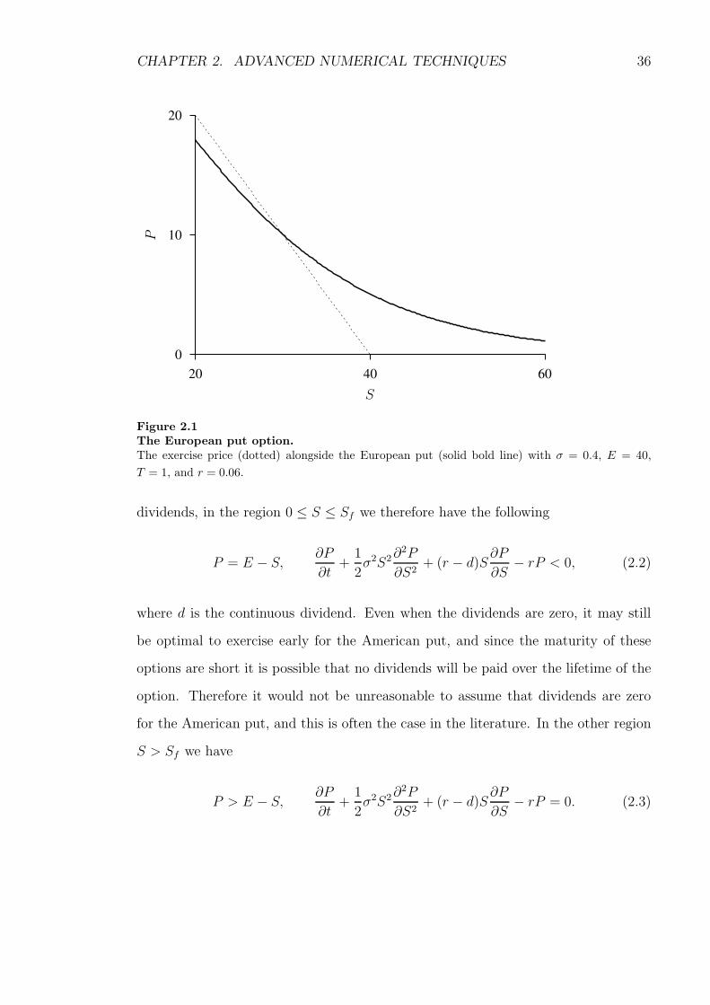
arguments must be used. In figure 2.1, the value of a typical European put is seen to
be lower than that of the payoff function (E − S) for some range of S. If this were
to be the price of the American put option P , then P (S, t) < E − S in this range. If
the option is bought, one would simply exercise it making an instant risk-free profit
of E − S − P (since P < E − S). Then, by arbitrage, the option price would move
so as an instantaneous profit could no longer be made. Consequently the following
constraint must hold for the American put;
P (S, t) ≥ max(E − S, 0). (2.1)
Now assume that there exists some point in S, say Sf , below which it is optimal
to exercise, but not so above. For the American put, the holder will exercise in the
region S < Sf . In this region, the return on a bank deposit is more than if the option
is held. Clearly, the solution in the region S < Sf does not need to be calculated
since we know that the option is exercised and therefore P = E − S.
In the region S > Sf , the BSM equation must still hold, but another condition
is needed in order to close the problem: the value of Sf must be chosen so as to
maximise the value of the option. This is found by examining the gradient of P
at the free boundary. We can show that ∂P/∂S = −1, i.e. the function P runs
smoothly into the payoff function (see figure 2.2). If ∂P/∂S < −1 then P < E − S
for some region close to Sf and we have already discussed earlier how this would not
be possible. For the case ∂P/∂S > −1, consider the strategy taken by the holder on
when to exercise. A holder would wish to allow the asset price drop as low as possible
before exercising, so if ∂P/∂S > −1 the value of the option near Sf can be increased
if we take a smaller value of Sf . We conclude, therefore, that the only possibility is
that ∂P/∂S = −1.
Assuming that the option is priced under the BSM framework with continuous
CHAPTER 2. ADVANCED NUMERICAL TECHNIQUES 36
20
10
0
604020
S
P
Figure 2.1The European put option.The exercise price (dotted) alongside the European put (solid bold line) with σ = 0.4, E = 40,
T = 1, and r = 0.06.
dividends, in the region 0 ≤ S ≤ Sf we therefore have the following
P = E − S, ∂P
∂t+
1
2σ2S2∂
2P
∂S2+ (r − d)S∂P
∂S− rP < 0, (2.2)
where d is the continuous dividend. Even when the dividends are zero, it may still
be optimal to exercise early for the American put, and since the maturity of these
options are short it is possible that no dividends will be paid over the lifetime of the
option. Therefore it would not be unreasonable to assume that dividends are zero
for the American put, and this is often the case in the literature. In the other region
S > Sf we have
P > E − S, ∂P
∂t+
1
2σ2S2∂
2P
∂S2+ (r − d)S∂P
∂S− rP = 0. (2.3)

CHAPTER 2. ADVANCED NUMERICAL TECHNIQUES 37
20
10
0
604020
S
Sf
P
Figure 2.2The American put option.The exercise price (dotted) alongside the American put (solid bold line) with σ = 0.4, E = 40,
T = 1, and r = 0.06. The American put option is exercised for S < Sf .
The boundary conditions at the free boundary are correspondingly
P (Sf(t), t) = E − Sf ,∂P
∂S(Sf(t), t) = −1. (2.4)
The final condition (location) for the free boundary must be found by asymptotic
analysis of the problem in the limit as we approach maturity. For the American put,
Kim (1990) finds the initial free boundary value to be
Sf (T ) = min[
E,r
dE]
. (2.5)
Hence for the American put with no dividend, the final condition is simply Sf(T ) = E.
Similar arguments lead to the following boundary conditions for an American
CHAPTER 2. ADVANCED NUMERICAL TECHNIQUES 38
call C,
C(S, T ) = max[S −E, 0] (2.6)
C(Sf (t), t) = Sf − E (2.7)
∂C
∂S(Sf(t), t) = 1 (2.8)
Sf(T ) = max[
E,r
dE]
. (2.9)
2.3 Asymptotic analysis of the American option
near expiry
Following the paper by Kuske and Keller (1998) using integral equations, both
Evans et al. (2002) and Widdicks et al. (2005) confirm the three tier structure to
the solution of the American put option using matched asymptotic expansions in the
limit as time tends to expiry. Furthermore, Evans et al. (2002) also includes analysis
of both call and put options with dividends. They find that the ratio between the
dividend and interest rate is important in determining the structure of both the
solution and the free boundary in the limit as time tends to zero. For the call, there
are three distinct cases dependent on this ratio. Firstly, when d = 0 the well known
case arises where it is never optimal to exercise and hence the American call is exactly
the same as the European call. Second, when 0 < d < r, the solution can be captured
with a simple structure, the boundary is O(τ12 ) around the limit of the free boundary
(as time tends to expiry). Finally, when d ≥ r the situation becomes more complex,
equivalent in fact to the structure of the American put option, the free boundary is
O
(
(
τ ln 1τ
)
12
)
and the solution exhibits a three tier structure. Roles are reversed for
the American put, with 0 ≤ d ≤ r the solution is the complex three tier structure,
and with d > r the solution is the simple structure.
In the next two subsections we will run through the equations detailing the struc-
ture for the two cases 0 < d < r and d ≥ r involving an American call. The analysis
used for a call when 0 < d < r is later used in chapter 7 for the delayed-exercise

CHAPTER 2. ADVANCED NUMERICAL TECHNIQUES 39
option.
2.3.1 The American call with 0 < d < r
In order to use the asymptotic analysis we must convert the BSM PDE to non-
dimensional form. Making the following substitutions
S = Eex, t = T − τ/1
2σ2, C(S, t) = S − E + Ee−ρτ c(x, τ),
with
ρ =r
12σ2
ν =d
12σ2
into (1.5) results in the following equation
∂c
∂τ=∂2c
∂x2+ (ρ− ν − 1)
∂c
∂x+ eρτ (ρ− νex), (2.10)
for x < xf (τ) where Sf(t) = Eexf (τ). Then the boundary conditions may be expressed
as:
c =∂c
∂x= 0 at x = xf (τ), (2.11)
c ∼ eρτ (1− ex) as x→ −∞, (2.12)
c = max(1− ex, 0) at τ = 0, (2.13)
From equations (2.10) to (2.13) we may confirm Kim’s (1990) limit of x0, the free
boundary as time tends to expiry. At expiry, we have that ∂2c/∂x2 = ∂c/∂x = 0 for
x > 0. Then (2.10) becomes
∂c
∂τ= ρ− νex for x > 0. (2.14)
Now in order to satisfy the constraint c ≥ max(1− ex, 0), we require that ∂c/∂τ > 0.
If we specify x0 = log(ρ/ν), then ∂c/∂τ > 0 for 0 ≤ x ≤ x0, and ∂c/∂τ < 0 for
x > x0. Clearly then we exercise in the region x > x0, so then xf (0) = x0, or
CHAPTER 2. ADVANCED NUMERICAL TECHNIQUES 40
Sf (T ) = rEd
in the original variables.
Both Wilmott et al. (1995) and Evans et al. (2002) show that the free boundary
here is of parabolic form. Let us consider the limit of small time behaviour near
expiry, letting τ = ǫT , with T = O(1) and ǫ a small parameter, we have the following
expansion for x < x0
c(x, τ) = max(1− ex, 0) + (ρ− νex)τ +O(ǫ2). (2.15)
This expansion can only satisfy one of the boundary (c = 0) conditions at x = xf ,
hence we require a separate region close to the free boundary to satisfy the derivative
condition, ∂c∂x
= 0. Let us introduce the following scalings
x = x0 + ǫ12X, c = ǫ
32 C, xf = x0 + ǫ
12L0
Then substituting these into (2.10) to O(ǫ12 ) we get the following:
∂C
∂T=∂2C
∂X2− ρX, (2.16)
with the conditions
C =∂C
∂X= 0 at X = L0(T ), (2.17)
C(X, 0) = 0, L0(0) = 0, (2.18)
C → −ρXT as X → −∞, (2.19)
where the third condition matches to the outer solution (2.15).
Then seeking a similarity solution of the form V = τ32g(ξ) where ξ = X/
√
T , and
L0 = ξ0√
T , we arrive at the following ODE;
g′′ +1
2ξg′ − 3
2g = ρξ, (2.20)

CHAPTER 2. ADVANCED NUMERICAL TECHNIQUES 41
with conditions
g(ξ0) = g′(ξ0) = 0, (2.21)
g(ξ) ∼ −ρξ as X → −∞. (2.22)
where the ξ0 is a constant. Then we see that the free boundary xf − x0 ∼ O(τ12 ).
Solving the ODE both Wilmott et al. (1995) and Evans et al. (2002) find the tran-
scendental equation for the problem to be
ξ30e
14ξ20
∫ ξ0
−∞e−
14s2
ds = 2(2− ξ20), (2.23)
and the constant ξ0 can be found using numerical methods to be
ξ0 = 0.9034 . . . (2.24)
Then in original variables we have that as t→ T
Sf (t) ∼rE
D0
(
1 + ξ0
√
1
2σ2(T − t) + . . .
)
. (2.25)
We note that the derivation here is independent of dividend payments except
for the location of the exercise boundary at expiry. Figure 2.3 diagrammatically
illustrates the structure of the solution near expiry. The solution is approximately
European to order O(τ 1/2) around x = 0, with the American element of the option
only coming into play in a smaller region also O(τ 1/2) around x0. Obviously, as time
to expiry increases the region around x = 0 will begin to interact with the region
around x0 and a more complex structure will arise. In the case when d ≥ r, x0 = 0
so that a complex structure prevails even in the limit as time tends to expiry. In the
next section we give a brief outline of the matched asymptotic expansions presented
by Evans et al. (2002) to demonstrate the three tier structure of the solution.

CHAPTER 2. ADVANCED NUMERICAL TECHNIQUES 42
x0xfx = 0
O(
τ12
)
O(
τ12
)
c(x, τ)
(a) Overview
x0 xf
O(
τ12
)
c(x, τ)
co(x, τ)
(b) Zoomed region
Figure 2.3The simple structure for an American call with 0 < d < r.The solid line shows the numerical solution for the American call with dividends. We can see the
solution has two parts, both order O(τ1/2), around x = 0 and x = x0. (a) shows the entire solution
space whilst (b) shows a zoomed region around x0 with the outer solution co (dashed). Parameters
here are T = 0.1, E = 40, r = 0.06, σ = 0.2, and d = 0.03, chosen so that x0 ≫√
τ .
2.3.2 Asymptotic analysis for the case d ≥ r
The free boundary in this case does not have a parabolic form, which can be
verified by setting xf (τ) ∼ ξ0√τ , and attempting to find a constant such that the
boundary conditions are satisfied. Since no constant can be found (ξ0 → ∞), the
solution is instead found to have a three tier structure.
If we look at the problem (2.10) with conditions (2.11) to (2.13) and look for a
solution in the limit of small time where τ = ǫT , we get
∂c
∂T= ǫ
[
∂2c
∂x2+ (ρ− ν − 1)
∂c
∂x+ eǫρT (ρ− νex)
]
. (2.26)
Then we look for a solution of the form
c(x, τ) = C0(x, T ) + ǫC1(x, T ) +O(ǫ2).
Then for x < 0 we have the O(1) problem
∂C0
∂T= 0, (2.27)
CHAPTER 2. ADVANCED NUMERICAL TECHNIQUES 43
with the condition
C0(x, 0) = 1− ex. (2.28)
Then we have that
C0(x, T ) = 1− ex. (2.29)
At O(ǫ) we have
∂C1
∂T=∂2C0
∂x2+ (ρ− ν − 1)
∂C0
∂x+ (ρ− νex), (2.30)
so using the above form for C0 we get
∂C1
∂T= ρ(1− ex), (2.31)
with the conditions
C1(x, T ) ∼ ρT (1− ex) as x→ −∞, (2.32)
C1(x, 0) = 0, (2.33)
so then we have the following expansion for c in the region x < 0
c(x, τ) = 1− ex + ρτ(1− ex) +O(ǫ2). (2.34)
We can now introduce a region around the free boundary of O(ǫ) to satisfy the
boundary conditions, x = xf(τ) + ǫz where z = O(1). Then we have
∂
∂τ→ 1
ǫ
∂
∂T− 1
ǫ2dxf (T )
dT
∂
∂z,
∂
∂x→ 1
ǫ
∂
∂z.
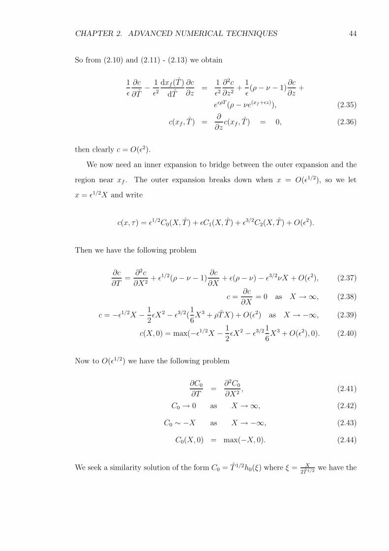
CHAPTER 2. ADVANCED NUMERICAL TECHNIQUES 44
So from (2.10) and (2.11) - (2.13) we obtain
1
ǫ
∂c
∂T− 1
ǫ2dxf (T )
dT
∂c
∂z=
1
ǫ2∂2c
∂z2+
1
ǫ(ρ− ν − 1)
∂c
∂z+
eǫρT (ρ− νe(xf +ǫz)), (2.35)
c(xf , T ) =∂
∂zc(xf , T ) = 0, (2.36)
then clearly c = O(ǫ2).
We now need an inner expansion to bridge between the outer expansion and the
region near xf . The outer expansion breaks down when x = O(ǫ1/2), so we let
x = ǫ1/2X and write
c(x, τ) = ǫ1/2C0(X, T ) + ǫC1(X, T ) + ǫ3/2C2(X, T ) +O(ǫ2).
Then we have the following problem
∂c
∂T=
∂2c
∂X2+ ǫ1/2(ρ− ν − 1)
∂c
∂X+ ǫ(ρ− ν)− ǫ3/2νX +O(ǫ2), (2.37)
c =∂c
∂X= 0 as X →∞, (2.38)
c = −ǫ1/2X − 1
2ǫX2 − ǫ3/2(
1
6X3 + ρTX) +O(ǫ2) as X → −∞, (2.39)
c(X, 0) = max(−ǫ1/2X − 1
2ǫX2 − ǫ3/2 1
6X3 +O(ǫ2), 0). (2.40)
Now to O(ǫ1/2) we have the following problem
∂C0
∂T=
∂2C0
∂X2, (2.41)
C0 → 0 as X →∞, (2.42)
C0 ∼ −X as X → −∞, (2.43)
C0(X, 0) = max(−X, 0). (2.44)
We seek a similarity solution of the form C0 = T 1/2h0(ξ) where ξ = X2T 1/2
we have the

CHAPTER 2. ADVANCED NUMERICAL TECHNIQUES 45
following problem
h′′0 + 2ξh′0 − 2h0 = 0, (2.45)
h0 ∼ −− 2ξ as X → −∞, (2.46)
h0 → 0 as X → +∞. (2.47)
which has the solution
h0 =1√πe−ξ2 − ξerfc(ξ). (2.48)
Next, to order O(ǫ) we have
∂C1
∂T=∂2C1
∂X2+ (ρ− ν − 1)
∂C0
∂X+ (ρ− ν), (2.49)
∂C1
∂X= 0 as X →∞, (2.50)
C1 ∼ −1
2X2 as X → −∞, (2.51)
C1(X, 0) =
−12X2 X ≤ 0
0 X > 0. (2.52)
Then we seek a solution of the form C1 = T h1(ξ) where again ξ = X2T 1/2
. Then we
obtain
h′′1 + 2ξh′1 − 4h1 = 2(1 + ν − ρ)h′0 + 4(ν − ρ), (2.53)
h1 ∼ −2ξ2 as X → −∞, (2.54)
h′1 → 0 as X →∞, (2.55)
which has the asymptotic form
h1 ∼ ρ− ν +1
2√π
(1 + ν − ρ)e−ξ2
ξas X →∞. (2.56)

CHAPTER 2. ADVANCED NUMERICAL TECHNIQUES 46
Next, to order O(ǫ3/2) we have
∂C2
∂T=∂2C2
∂X2+ (ρ− ν − 1)
∂C1
∂X− νX, (2.57)
∂C2
∂X= 0 as X →∞, (2.58)
C2 ∼ −1
6X3 − ρXT as X → −∞, (2.59)
C2(X, 0) =
−16X3 X ≤ 0
0 X > 0. (2.60)
Then we seek a solution of the form C2 = T 3/2h2(ξ) where again ξ = X
2T 1/2 . Then we
obtain
h′′2 + 21
2ξh′2 − 6h2 = 2(1 + ν − ρ)h′1 + 8νξ, (2.61)
h2 ∼ −4
3ξ3 − 2ρξ as X → −∞, (2.62)
h′2 → 0 as X →∞, (2.63)
which has the asymptotic form
h2 ∼ −2νξ +1
4√π
(1 + ν − ρ)2e−ξ2
as X →∞. (2.64)
The solution in this region is
c(x, τ) = τ 1/2h0
(
x
2√τ
)
+ τh1
(
x
2√τ
)
+ τ 3/2h2
(
x
2√τ
)
+ . . . . (2.65)
with the asymptotic behaviour as ξ →∞:
h0 ∼1
2√π
e−ξ2
ξ2+ . . . , (2.66)
h1 ∼ (ρ− ν) + . . . (2.67)
h2 ∼ −2νξ + . . . (2.68)
Then matching in the region of O(τ) around the free boundary using (2.65) and

CHAPTER 2. ADVANCED NUMERICAL TECHNIQUES 47
xfx = 0
O(
τ12
)
O (τ)
O(
(
τ ln(1/τ))
12
)
c(x, τ)co(x, τ)
Figure 2.4The simple structure for an American call with d ≥ r.The solid line shows the numerical solution for the American call with dividends, the dashed line
shows the asymptotic outer solution. We can see the solution has three interacting regions, around
x = 0, x = xf and in between. Parameters here are T = 0.1, E = 40, r = 0.06, σ = 0.2, and
d = 0.06.
(2.68), we obtain the two following transcendental equations
1
2√πτe−x2
f /4τ + ρ− ν ∼ 0, ρ < ν,
1
4√πτe−x2
f/4τ − ν ∼ 0, ν = ρ. (2.69)
Then in the original variables we have the following formula for the free boundary
as τ → 0
Sf (t) ∼ E + Eσ√
(T − t) ln[σ2/(8π(T − t)(r − d)2)], r < d
Sf(t) ∼ E + Eσ
√
2(T − t) ln[1/(4√πd(T − t))], r = d. (2.70)
CHAPTER 2. ADVANCED NUMERICAL TECHNIQUES 48
2.3.3 The American put with dividends
For the American put option, Evans et al. (2002) find that the free boundary has
a parabolic solution for r > d, and the parabolic logarithmic solution for r ≤ d. In
the limit as time tends to expiry we have that
Sf(t) ∼ E − Eσ√
(T − t) ln[σ2/(8π(T − t)(r − d)2)], r > d
Sf (t) ∼ E − Eσ√
2(T − t) ln[1/(4√πd(T − t))], r = d,
Sf(t) ∼dE
r
(
1− ξ0√
1
2σ2(T − t) + . . .
)
, r < d. (2.71)
2.4 Numerical Techniques and extensions
It is not normally the case that an analytical solution can be found for free bound-
ary problems (which are inherently nonlinear) and so we generally require a numerical
method in order to solve them. One method is to write the free boundary problem
in terms of a body-fitted coordinate system, in which we simultaneously solve for the
free boundary, explained later in section 2.4.3. This results in a relatively simple,
albeit non-linear PDE in the single asset case, but is much more difficult to imple-
ment with an increase in the number of assets. The method also relies on the free
boundary being a smooth continuous function that does not disappear at any stage.
For instance, to price a Bermudan option (relatively simple by other methods) the
free boundary is only defined at the exercise dates. A body-fitted coordinate system
is not appropriate in this instance, so a more robust method (over a fixed domain) in
which the boundary conditions are implicitly satisfied in the new set of equations is
then necessary. Crank (1984) describes two such formulations that can be applied to
the heat equation; the enthalpy method and variational inequalities (see Elliot and
Ockendon, 1982 for a detailed description). The variational inequality formulation
is the most appealing for finance problems (since there is no obvious equivalent con-
dition in financial terms to the overall conservation of heat). Wilmott et al. (1993)
have used the methods described by Crank (1984) to formulate the American option
CHAPTER 2. ADVANCED NUMERICAL TECHNIQUES 49
as a variational inequality.
The American Option as a Variational Inequality
We have already formulated the American option earlier in this section. It is
now simple to formulate this as a parabolic variational inequality, and then after
discretisation, a linear complementary problem. If we let LBSM be the standard
BSM operator, and G(S, t) be the constraint applied to the problem, the value of
early exercise, then we can write (2.1)–(2.4) as
LBSM
{
V (S, t)}
·(
V (S, t)−G(S, t))
= 0, LBSM
{
V (S, t)}
≤ 0, V (S, t)−G(S, t) ≥ 0,
(2.72)
such that V and ∂V/∂S are continuous. Note here that for the American put,
G(S, t) = max(E − S, 0), and consequently its derivative is discontinuous at S = E.
However, it can be shown that V (S = E, t) > G(S = E, t) for any time before expiry
so the constraint will never be applied there. This is not always the case, as for
example in the case of the cash-or-nothing American option, there is a discontinuous
constraint, implying that the free boundary is known a priori, since it is always opti-
mal to exercise at the strike price. The smooth-pasting condition therefore does not
apply, since G(Sf , t) and ∂G(Sf , t)/∂S are not continuous at the strike price.
Elliot and Ockendon (1982), Friedman (1988) and Kinderlehrer and Stampacchia
(1980) give detailed accounts of the existence and uniqueness proof for variational
inequalities of this form, which involves knowledge of abstract functional analysis;
the problem is basically reduced to minimising a convex set of functions.
2.4.1 The PSOR Method
First the problem is discretised according to the Crank-Nicolson method. Since
the problem is backwards parabolic, for convenience we make the substitution τ =
T − t so that the problem is now forward in τ . Now discretise the problem so that
∆S =Smax
n, ∆τ =
T
m, V (i ·∆S, k ·∆τ) = uk
i ,
CHAPTER 2. ADVANCED NUMERICAL TECHNIQUES 50
then we can write an approximation to the BSM operator as
αiuk+1i−1 + (1/∆t+ βi)u
k+1i + γiu
k+1i+1 = −αiu
ki−1 + (1/∆t− βi)u
ki − γiu
ki+1, (2.73)
where uk is known and uk+1 must be found. The errors in this scheme are of the order
O(∆S2,∆τ 2). The coefficients α, β and γ are defined in the introduction section 1.3.3.
Next, let G(i ·∆S, k ·∆t) = gki , then the early exercise constraint can be written as
uki ≥ gk
i , for k ≥ 1 and ∀i, (2.74)
and so the discretised problem is
(
αiuk+1i−1 + (1/∆t+ βi)u
k+1i + γiu
k+1i+1 − Zk
i
)
·(
uk+1i − gk+1
i
)
= 0, (2.75)
where we have defined
Zki = −αiu
ki−1 + (1/∆t− βi)u
ki − γiu
ki+1.
The boundary conditions can be determined explicitly so that
uk0 = Zk
0 ,
ukn = Zk
n,∀k. (2.76)
For example, the boundary conditions on the American put give Zk0 = E and Zk
n = 0.
Hence, discretisation leads to a succession of elliptic variational inequalities to be
solved at each time step. Such inequalities can be expressed in the general linear
complementarity (vector) form
AB = 0, A ≥ 0, B ≥ 0. (2.77)
where the product here implies that at least one element in A and B must be zero at
every position.

CHAPTER 2. ADVANCED NUMERICAL TECHNIQUES 51
Many methods have been proposed to solve such a problem when
A = Ax− b,
and
B = x,
where x is the n-vector to be determined, b is a known n-vector and A is an n × n
matrix. Generic methods for solving such a system of equations are not geared toward
finite-difference formulation, so by adapting the SOR method Cryer (1971) was able
to exploit the sparseness of matrix A.
Now, let uk and g denote the vectors as follows
uk =
xk1
...
xkn−1
, gk =
gk1
...
gkn−1
. (2.78)
The values at the boundary are not included, since we do not need to iterate over
them. We can then construct a matrix A and a vector bk such that we can rewrite
(2.75), as the linear complementarity problem
(
Auk+1 − bk
)
·(
uk+1 − gk+1
)
= 0, (2.79)
where the product represents the set of equations such that either the first bracket
or the second bracket is zero.
We now define the Projected Successive Over Relaxation algorithm, or PSOR. It
is basically an extension of the SOR method, modified to solve the linear complemen-
tary problem. Crank (1984) notes that although the PSOR method has been used
heuristically as far back as Christopherson and Southwell (1938), convergence was
not proved rigorously until Cryer (1971).

CHAPTER 2. ADVANCED NUMERICAL TECHNIQUES 52
In the SOR method we have
yk+1,q+1i = 1
1/∆t+βi
(
Zki − αiu
k+1,q+1i−1 − γiu
k+1,qi+1
)
, (2.80)
uk+1,q+1i = uk−1,q
i + ω(yk+1,q+1i − uk+1,q
i ), (2.81)
where q represents the qth iteration. If we iterate using equations (2.80) and (2.81)
over the domain until successive iterates are sufficiently close to one another, then u
will satisfy the first constraint of the problem Auk+1 = bk. Then we must modify
the algorithm to satisfy the constraint that uk+1 ≥ gk+1. This is undertaken by
modifying the second step in the SOR algorithm (2.81) to obtain the projected SOR
algorithm:
yk+1,q+1i = 1
1/∆t+βi
(
Zki − αiu
k+1,q+1i−1 − γiu
k+1,qi+1
)
, (2.82)
uk+1,q+1i = max
[
uk+1,qi + ω(yk+1,q+1
i − uk+1,qi ), gk+1
i
]
. (2.83)
We then iterate over these two equations until the difference between successive iter-
ations is sufficiently small.
The problem is reduced to maximising the vector uk+1 over the solution space.
This can be interpreted in finance terms as choosing the free boundary in order to
maximise the value of the option.
2.4.2 Modifying PSOR - A Novel Approach
We define Block SOR to be a modified SOR method in which the vectors uk+1, A
and bk are partitioned into smaller subsets, over which we solve (with a direct method)
while all other points are constant. This method is well known and is particularly
efficient when solving multi-dimensional problems.
If timesteps are large, and parameter σ is large, the rate of convergence for the
PSOR scheme can be very slow, especially when extended to the multi-asset problem.
We can take advantage of some of the properties of the free boundary in order to
make the PSOR solver converge much quicker. We know that for the American put,
CHAPTER 2. ADVANCED NUMERICAL TECHNIQUES 53
the value of the free boundary is monotonically decreasing. Consequently, at step
k + 1, let us partition uk+1 into the subsets
uk+11 =
xk1
...
xkak−1
, uk+12 =
xkak
...
xkn−1
, (2.84)
where ak ·∆S is the position of the free boundary at time k on the grid. We can also
construct the corresponding subsets A1, A2, bk1, and bk
2. Due to the monotonicity of
the free boundary we know that for a put
ak+1 ≤ ak,
whilst for a call
ak+1 ≥ ak.
Thus, when pricing a put, we know with certainty that uk+12 is not exercised, implying
that we may solve this subset using a direct method, since no projection is required,
but for the other subset uk+11 , point PSOR is still used. We define this new algorithm
to be the Advanced PSOR scheme, or APSOR. If there were a large number of
iterations at each time step then iterating with the direct solver would become slow
and inefficient. However, due to the fact that the boundary rarely moves more than
one or two nodes in any one time step, and often stays at the same node, the number
of necessary iterations is small (there is no need to iterate at all if the free boundary
does not move).
Figures 2.5 and 2.6 give a brief description of the algorithms needed to generate the
APSOR. The function ’TridiagonalSolver’ (an adaptation of the Thomas algorithm)
is a modified tridiagonal solver for the region [a + 1, n]. The result can then be
over relaxed (if optimal to do so) and an error over the region calculated. Then
function ‘PointSolverDown’ is called, which solves over the region [1, a]. The solver
moves downward, starting at a, because once the option is exercised at if , we know

CHAPTER 2. ADVANCED NUMERICAL TECHNIQUES 54
AdvancedPsorSolver(freeBoundary, u, g)1 ComputeScheme(alpha, beta, gamma, z)2 while error > tol3 do4 a← freeBoundary5 TridiagonalSolver(a, alpha, beta, gamma, z, u, error)6 freeBoundary ← PointSolverDown(a, error, alpha, beta, gamma, z, u, g)7 return loops
Figure 2.5Advanced PSOR solver – pseudo codeThe algorithm performed at each time step. Values of ‘alpha’, ‘beta’, ‘gamma’ and ‘z’ come from
(2.73), and TridiagonalSolver uses Gaussian elimination. ‘loops’ is returned for optimisation.
PointSolverDown(a, error, alpha, beta, gamma, z, u, g)1 for i← a to 12 do3 y ← SOR(alpha, beta, gamma, z, u)4 if y ≤ gi
5 then6 ui ← gi
7 break8 else9 error ← error + (y − ui) ∗ (y − ui)
10 ui ← y11 return i
Figure 2.6Point Solver Down – pseudo codeThe “search” type algorithm (that also updates the solution) to find the next approximation to the
free boundary.
that it will be exercised for all i < if (we are assuming here that the option is the
American put for these conditions to hold). This implies that once the condition is
satisfied we can break the ‘for’ loop as the solution will not change in the remainder
of the region. If the free boundary is stationary (with respect to the nodes) then
the condition is satisfied at a and the solution has already been found, and no more
iteration is required.
It is trivial to modify the algorithm to solve a problem where the free boundary is
strictly increasing, but it can also be modified to solve problems where the movement
of the boundary is unknown, or changes direction, so long as we know an approximate

CHAPTER 2. ADVANCED NUMERICAL TECHNIQUES 55
start point and that the boundary is a single point. For example, in figure 2.6, if
the algorithm breaks when i = a, it may be possible that the free boundary is in the
region [a + 1, n]. So when a break occurs at a we must then move upward through
the solution space, using PSOR, checking for the first point at which the condition is
not satisfied. The last point at which it has been satisfied is passed out as the free
boundary.
2.4.3 The Boundary-fitted Coordinate Formulation
The body-fitted coordinate (BFC) method is an alternative means to solve the
American option problem. As mentioned earlier, it is relatively simple to formulate
with a single underlying asset, however the complexity increases dramatically each
time we increase the number of assets. For the single asset case, we may usefully use
the BFC to test the accuracy of our PSOR method.
The BFC uses a transformation in order to solve the moving boundary problem
over a fixed coordinate system. While Landau (1950) was the first to propose such
a transformation, Crank (1957) was the first to apply it to a finite-difference scheme
to solve diffusion equations, then more recently Widdicks (2002) adapted the scheme
to solve the American option problem. Smooth convergence of the method in both
S and t, enabled Widdicks (2002) to use Richardson extrapolation of the results to
improve accuracy, resulting in a highly accurate method.
The advantage of the BFC method is this: the position of the free boundary is
solved accurately at each time step, which is important in finance since the holder
of the option will need to know precisely when it is optimal to exercise. The PSOR
scheme will calculate the position of the free boundary to O(∆S), whereas we would
expect the BFC to position the boundary to O((∆S)2). Although we have accuracy
at the free boundary, when we wish to calculate the solution at some prescribed
point in S space, then we will almost certainly not have a grid point located at this
position, although the value can then be found easily using interpolation. This is a
minor drawback as an inaccurate location of the boundary can easily lead to larger
CHAPTER 2. ADVANCED NUMERICAL TECHNIQUES 56
errors.
Widdicks (2002) notes that BFC has difficulty tracking the free boundary when
the time to expiry is small (as do many of the numerical methods for solving American
options). For the scheme to converge, the timesteps may be altered so that they are
smaller when the time to expiry is small, and larger when the time to expiry is large.
The rate at which they are scaled is chosen to be τ12 so as to mimic (approximately)
the behaviour of the free boundary near expiry (c.f. section 2.3). For this reason,
section 2.5 outlines a new procedure that combines the ‘curtailed range’ analysis
used by Andricopoulos et al. (2004) on lattice methods, with the BFC, to arrive at a
scheme which is both accurate and does not have restrictions on the size of the time
steps.
Here the method as used by Widdicks (2002) is first explained. In the BFC,
the coordinate system is allowed to move with the free boundary. Again we use the
transformation τ = T − t, and in the case of the American put, we use the following
transformation for S,
S = S − Sf(τ), (2.85)
where S ∈ [0,∞] and S = Sf(t) ⇒ S = 0. The Black-Scholes equation under this
transformation then becomes
∂V
∂τ− dSf
dτ
∂V
∂S=
1
2σ2(S + Sf)
2∂2V
∂S2+ r(S + Sf)
∂V
∂S− rV. (2.86)
The PDE (2.86) is clearly non-linear, but we can use Newton iteration in order
to linearise the PDE; this involves making a guess at the solution, and assuming the
correction to the guess is small, say O(δ), then we can write
Vk+1,(q+1)i = V
k+1,(q)i + δVi,
Sk+1,(q+1)f = S
k+1,(q)f + δSf . (2.87)

CHAPTER 2. ADVANCED NUMERICAL TECHNIQUES 57
Then using a Crank-Nicolson scheme, we have (for example) the following approxi-
mations,
∂V
∂τ(S, τ +
1
2∆τ) ≈ 1
∆t(V k+1
i + δVi − V ki ),
Sf(τ +1
2∆τ) ≈ 1
2(Sk+1
f + δSf − Skf ). (2.88)
Then substituting (2.88) along with other terms into (2.86) we have a collection of
O(δ) and O(1) terms. Then collecting the O(δ) terms on the left hand side and the
O(1) terms on the right we arrive at an equation of the form,
δVi−1αi + δViβi + δVi+1γi + δSfθi = ǫi. (2.89)
This represents a tri-diagonal system but it also includes an extra column corre-
sponding to δSf . This can be readily solved using Gaussian elimination to find the
correction terms. We may iterate at each time level until the maximum correction
term is less than some prescribed tolerance,
max |δVi, δSf | ≤ tol, tol > 0.
2.5 An Improved Numerical Technique
As stated previously in section 2.4.3, the BFC method struggles to cope with the
free boundary as time tends toward expiry. However, Johnson (2003) finds that in
a problem with two free boundaries that converge to the same point at expiry, the
BFC on such a problem can track both of the boundaries even in this limit. If there
exists some way of defining an upper (lower) boundary on the solution for a put (call)
the problem can be formulated with one free boundary and one known boundary. If
the two boundaries converge to the same point, then any difficulties experienced with
tracking the boundary near expiry will be overcome, although the nodes are equally
spaced in the transformed space, the distance between nodes in real space will tend
CHAPTER 2. ADVANCED NUMERICAL TECHNIQUES 58
become increasingly small (a very positive feature) near expiry.
Andricopoulos et al. (2004) suggest that the ‘curtailed range’ technique can be
applied to both lattice and finite-difference grid methods. However, this suggestion
involves discounting nodes over which the solution is obtained, rather than fitting the
coordinate system around the curtailed range. The range suggested by Andricopoulos
et al. (2004) is
Smin = min[
S0erτ−ξσ
√τ , Ee−rτ−ξσ
√τ , 0]
, (2.90)
Smax = max[
S0erτ+ξσ
√τ , Ee−rτ+ξσ
√τ]
, (2.91)
where ξ is a parameter that the user defines and will effect the accuracy of the
scheme. Such a region can be thought of as follows: for a put, given St ∈ [Smax,∞],
the probability that a random walk followed by the asset will finish at time T in a
position to be exercised is set to be so small that it is not even worth calculating. The
parameter ξ measures how many standard deviations in the normal distribution it will
be from the mean, and hence increasing ξ will make the probability ever smaller and
accuracy will be increased. This is corroborated by the asymptotic analysis by Evans
et al. (2002) (for the singular perturbation analysis see also Widdicks et al., 2005), in
which the solution is found to have three distinct regions, and above the upper most
region, approximately of order τ12 , the American put option price is approximately
zero.
The upper-bound, Smax = U(τ) is specified for the American put option, and is
U(τ) = min[
Eeξσ√
τ , λE]
. (2.92)
The −rτ term is dropped from (2.91) so that U(τ) > E, and λ is some constant that
defines the maximum value of the grid required. The constant ξ is taken to be 10,
somewhat larger than the value suggested by Andricopoulos et al. (2002) in order to

CHAPTER 2. ADVANCED NUMERICAL TECHNIQUES 59
make sure the domain is of sufficient extent. For the American call, we set
L(τ) = max[
Ee−ξσ√
τ , 0]
, (2.93)
where L here is a lower bound.
Now, if we define F (τ) = L(τ) to be the lower boundary, and the function G(τ) =
U(τ)− F (τ) to be the difference between the upper and lower boundaries. Then the
mapping [Smin, Smax]→ [0, 1] is defined as follows
S =S − F (τ)
G(τ). (2.94)
Here the initial transformation is independent of the type of option. We must now
specify F and G subject to the option for which we are solving. For the American
put, U is known and given by (2.92), F (τ) = Sf(τ) is the free boundary, and therefore
G(τ) = U(τ)− Sf (τ). For a call, F (τ) = L(τ) is the known boundary, U(τ) = Sf (τ)
corresponds to the free boundary, and so G(τ) = Sf(τ) − L(τ). It can be now seen
why using this transformation will be accurate. Other methods struggle as time tends
to expiry, because ∆S cannot be set small enough to fully capture the solution in
this limit. Here, however, as time tends to expiry, G(τ)→ 0, and so ∆S = G∆S → 0
as well. Since we are discretising over ∆S, and the scheme is O(∆S2,∆τ 2), as we
approach expiry the scheme becomes very accurate in ∆S, no matter how small the
time to expiry is, as the corresponding ∆S is also reduced.
Now using (2.94) on the Black-Scholes equation we obtain;
Vτ −1
G(SGτ + Fτ )VS =
1
2σ2
(
S +F
G
)2
VSS + r
(
S +F
G
)
VS − rV. (2.95)
This equation is solved over S ∈ [0, 1]. Note here that when solving for a put, both
F and G are unknown functions (G is a known plus an unknown function), so both
must be solved, thus making the problem slightly more complicated than the previous
BFC formulation. For the call, however, F is a known function and we need only
solve for G.
CHAPTER 2. ADVANCED NUMERICAL TECHNIQUES 60
The boundary conditions for the put are as follows
F (0) = min
[
E,rE
d
]
,
V (S, 0) = max[E − S, 0],
V (0, τ) = E − F (τ),∂V
∂S(1, τ) = −G(τ),
V (1, τ) = 0, F (τ) +G(τ) = U(τ), (2.96)
and similarly for the call we have
U(0) = max
[
E,rE
d
]
,
V (S, 0) = max[S −E, 0],
V (0, τ) = 0,
V (1, τ) = G(τ) + F (τ)− E, ∂V
∂S(1, τ) = G(τ). (2.97)
2.5.1 The Advanced Body-Fitted Coordinated Method (ABFC)
To price a put, we must solve equation (2.95) subject to the boundary conditions
(2.96). This is a non-linear PDE, and so we use the Newton method as described in
section 2.4.3 to linearise the problem. This is slightly different to the BFC formula-
tion, since there is an extra equation that determines the value of G. Using a guess
such as that in (2.87) and discretising according to the Crank-Nicolson method, we
obtain a scheme of the form,
δVi−1αi + δViβi + δVi+1γi + δFθi + δGφi = ǫi, (2.98)
where ǫi contains the O(1) terms. If there are n nodes in S space over which to
solve, along with F and G, we have n + 2 unknowns, and correspondingly there are
n + 2 equations. From (2.96), there are four boundary conditions which will result
in a problem with n + 2 equations as required. The form of the system which must
be solved is of a tridiagonal format with two extra columns. This too can be solved

CHAPTER 2. ADVANCED NUMERICAL TECHNIQUES 61
simply by Gaussian elimination.
For the call, the scheme is of a similar form to that of the BFC,
δVi−1αi + δViβi + δVi+1γi + δGφi = ǫi. (2.99)
In fact, the format of the matrix is identical to when the problem is posed in the BFC
formulation, the coefficients for the BFC and ABFC are given in Appendix A.1.
2.6 Results
One of the reasons Widdicks (2002) cites for the use of the BFC method is the
smooth convergence obtained. Figure 2.7 shows the rate of convergence using both
the PSOR and the BFC methods. The PSOR method, has two sources of non-linear
error, both from the position of the free-boundary, and from the position of the
discontinuity at expiry. The discontinuity error at expiry is the larger component,
and causes the (magnified) oscillations shown in figure 2.7(b). If we choose n correctly
(such as placing a node at the strike price), we can avoid this error. Widdicks et al.
(2002) show that when pricing using lattice methods the oscillations are in fact a
function of the distance between the (nearest) node and the discontinuity at expiry.
This assumes that we know the position of the discontinuity and that it is constant
over the duration of the option. Widdicks (2002) also shows that this is the case
for finite-difference grids. However, the true positioning of the free boundary is not
constant with respect to grid position over time, so the PSOR method over or under
estimates the position of the free boundary. Since we cannot expect to know the
extent to which the PSOR method over or under estimates the position of the free
boundary, a clever extrapolation of the PSOR results is not possible.
Table 2.1 shows relative RMS errors for the four methods described in this chapter.
The RMS errors are calculated over 8 put options, with different exercise prices,
volatilities and expiry times. First compare the fixed grid methods to the boundary-
tracking grids methods. Both sets of results have been improved using Richardson

CHAPTER 2. ADVANCED NUMERICAL TECHNIQUES 62
4.485
4.4855
4.486
4.4865
4.487
0 250 500 750 1000
Number of nodes (n)
V(S
=36,0
)
(a) BFC
4.4775
4.48
4.4825
4.485
4.4875
0 250 500 750 1000
Number of nodes (n)
V(S
=36,0
)
(b) PSOR
Figure 2.7ConvergenceConvergence for the BFC method and the PSOR method. Here T = 1, S0 = 36, σ = 0.2, r = 0.06
and E = 40.
extrapolation. The values of n are chosen for the fixed grid methods so that a node
is placed at the strike price, hence non-linearity error at expiry is not present. The
results for the PSOR method are poor, and do not work optimally with Richardson
extrapolation, since the convergence is not monotonic, unlike that for BFC method.
To gain comparable accuracy to the BFC method, 4 or 5 times as many points need
to be used in the PSOR method.
The PSOR method also suffers from a slow rate of iterative convergence, so slow in
fact that it can sometimes appear not to converge. If the volatility σ is large, and ∆S
is small, then the number of iterations required to gain a sufficient level of accuracy
can run into the hundreds. The method seems to struggle when the free boundary is
O(√
τ log( 1τ)) rather than O(τ 1/2). When solving for an American call with dividends
(the boundary is O(τ 1/2) when 0 < d ≤ r, see section 2.3), the solver converges far
quicker than for the put, which has the O(√
τ log( 1τ)) boundary. When the size of
the timestep is reduced, the rate at which the number of iterations required falls
linearly. Using the APSOR reduces the computation time by taking advantage of the
monotonically decreasing (increasing) nature of the free boundary for the American
put (call). The Newton method is a fast converging method, typically only taking
less than 10 iterations to gain the required accuracy. This then explains why the
computation time for the PSOR increases faster than the BFC when ∆S is reduced,
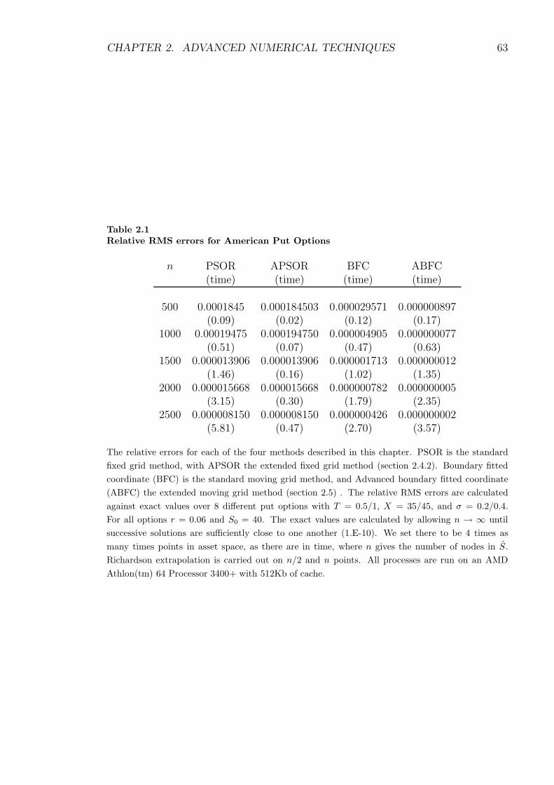
CHAPTER 2. ADVANCED NUMERICAL TECHNIQUES 63
Table 2.1Relative RMS errors for American Put Options
n PSOR APSOR BFC ABFC(time) (time) (time) (time)
500 0.0001845 0.000184503 0.000029571 0.000000897(0.09) (0.02) (0.12) (0.17)
1000 0.00019475 0.000194750 0.000004905 0.000000077(0.51) (0.07) (0.47) (0.63)
1500 0.000013906 0.000013906 0.000001713 0.000000012(1.46) (0.16) (1.02) (1.35)
2000 0.000015668 0.000015668 0.000000782 0.000000005(3.15) (0.30) (1.79) (2.35)
2500 0.000008150 0.000008150 0.000000426 0.000000002(5.81) (0.47) (2.70) (3.57)
The relative errors for each of the four methods described in this chapter. PSOR is the standard
fixed grid method, with APSOR the extended fixed grid method (section 2.4.2). Boundary fitted
coordinate (BFC) is the standard moving grid method, and Advanced boundary fitted coordinate
(ABFC) the extended moving grid method (section 2.5) . The relative RMS errors are calculated
against exact values over 8 different put options with T = 0.5/1, X = 35/45, and σ = 0.2/0.4.
For all options r = 0.06 and S0 = 40. The exact values are calculated by allowing n → ∞ until
successive solutions are sufficiently close to one another (1.E-10). We set there to be 4 times as
many times points in asset space, as there are in time, where n gives the number of nodes in S.
Richardson extrapolation is carried out on n/2 and n points. All processes are run on an AMD
Athlon(tm) 64 Processor 3400+ with 512Kb of cache.

CHAPTER 2. ADVANCED NUMERICAL TECHNIQUES 64
100 200
300 400
200 400
600 800
1000 1.01395
1.014
1.01405
1.0141
1.01415
1.0142
nm
V (S = E, 0)
(a) ∆τ = (T − t)/n
100 200
300 400
200 400
600 800
1000 1.01395
1.014
1.01405
1.0141
1.01415
nm
V (S = E, 0)
(b) ∆τ ∼ (T − t)1/2/n
Figure 2.8Convergence for different time stepsConvergence for an at-the-money American put option w.r.t. m number of nodes in τ space and n
number of nodes in S. Parameters are chosen to exaggerate the effects: σ = 0.4, r = 0.05, E = 10,
and T = 1.
even though the PDE we solve is more complicated than that for the PSOR method.
The ABFC method is stable even for large timesteps. Figure 2.8 shows the rate
of convergence for various combinations of nodes in S and τ for the ABFC method.
Figure 2.8(a) shows results obtained by discretising in the usual manner, with con-
stant timesteps across time. Figure 2.8(b) has results obtained using scaled timesteps
such as those employed to improve stability in the BFC method. Clearly, bunching
the timesteps near expiry improves accuracy, and unlike the the PSOR method (re-
ducing the timesteps has little effect on the computation time due to the increase in
iterations required) using a small number of timesteps will greatly improve efficiency
of the scheme.
Figure 2.9 gives a graphical representation of how much more accurate the ABFC
is compared to the PSOR and even BFC methods at tracking the free boundary. The
value of ∆S in the PSOR is the same as that of ∆S in the BFC, suggesting that
the BFC can only track the boundary to O(∆S) as we approach expiry. The ABFC
however is at the value that has been predicted by the asymptotic analysis carried
out by Kuske and Keller (1998).
Tables 2.1 and 2.2 show the high accuracy of the ABFC method. In table 2.1 we
see that for only a small increase in computation time, accuracy is increased (w.r.t.
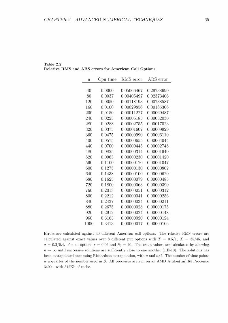
CHAPTER 2. ADVANCED NUMERICAL TECHNIQUES 65
Table 2.2Relative RMS and ABS errors for American Call Options
n Cpu time RMS error ABS error
40 0.0000 0.05066467 0.2973869080 0.0037 0.00405497 0.02373406120 0.0050 0.00118193 0.00738587160 0.0100 0.00029856 0.00185306200 0.0150 0.00011227 0.00069487240 0.0225 0.00005183 0.00032030280 0.0288 0.00002755 0.00017023320 0.0375 0.00001607 0.00009929360 0.0475 0.00000990 0.00006110400 0.0575 0.00000655 0.00004044440 0.0700 0.00000445 0.00002748480 0.0825 0.00000314 0.00001940520 0.0963 0.00000230 0.00001420560 0.1100 0.00000170 0.00001047600 0.1275 0.00000130 0.00000802640 0.1438 0.00000100 0.00000620680 0.1625 0.00000079 0.00000485720 0.1800 0.00000063 0.00000390760 0.2013 0.00000051 0.00000312800 0.2212 0.00000041 0.00000256840 0.2437 0.00000034 0.00000211880 0.2675 0.00000028 0.00000175920 0.2912 0.00000024 0.00000148960 0.3163 0.00000020 0.000001241000 0.3413 0.00000017 0.00000106
Errors are calculated against 40 different American call options. The relative RMS errors are
calculated against exact values over 8 different put options with T = 0.5/1, X = 35/45, and
σ = 0.2/0.4. For all options r = 0.06 and S0 = 40. The exact values are calculated by allowing
n → ∞ until successive solutions are sufficiently close to one another (1.E-10). The solutions has
been extrapolated once using Richardson extrapolation, with n and n/2. The number of time points
is a quarter of the number used in S. All processes are run on an AMD Athlon(tm) 64 Processor
3400+ with 512Kb of cache.

CHAPTER 2. ADVANCED NUMERICAL TECHNIQUES 66
9
9.2
9.4
9.6
9.8
10
0.010.0050
τ
Sf(τ
)
(a) Large time to expiry
9.8
9.9
10
2.e-41.e-40
τ
Sf(τ
)
(b) Small time to expiry
Figure 2.9The free boundary - BFC vs. PSOR vs. ABFCThe free boundary for the three different methods. (a) The BFC (dashed), the PSOR (solid step-like)
and the ABFC (solid) shown together. (b) The free boundary for PSOR (triangle), BFC (circle),
and ABFC (square). The asymptotic value is shown by the solid line.
RMS errors) by a factor of 100 on the (already very accurate) BFC solver. In table 2.2
the RMS and ABS relative errors are shown for a range of 40 call options. The results
are comparable to those tabled by Broadie and Detemple (1996). The exact solution
has been calculated by setting n = 15000, and is correct to the accuracy shown by
Broadie (1996). The number of time points is set to be a quarter of the number of
the points in S since the errors proportional to ∆S are larger (c.f. figure 2.8). We
can see that to obtain an ABS error of less than 0.1% we need just 200 points in S
with 50 time steps.
2.7 Conclusions
The contribution of this chapter has been two-fold. First, the monotonicity of
the free boundary has been exploited to improve the efficiency of the PSOR method.
This is important in the next chapter when the number of underlying assets is in-
creased, the use of finite-difference methods on 3 or 4 assets is highly dependent on
the efficiency of the algorithm. With some intuition regarding the whereabouts of the
free boundary, computation times can be reduced ten-fold. Secondly, the body-fitted
coordinate solver, fitted to an appropriate upper and lower bound, has impressive

CHAPTER 2. ADVANCED NUMERICAL TECHNIQUES 67
accuracy and efficiency. If it were possible to extend the method to the multi-asset
case, the reduction in nodes needed for high accuracy will help to maintain efficiency.
However the complex topology of the problem renders this extremely difficult if not
impossible.

Chapter 3
Multi-Asset American Options
A natural development in option pricing theory has been to extend the number
of assets on which options depend. There are numerous types of options on multiple
assets that have been proposed, some of which are listed below to set the scene for
discussion in the rest of the chapter. Most are bracketed under the umbrella term
rainbow options, the only exception listed below being the basket option.
Min-max options
The maximum option allows the holder to choose to exercise the best performing
of two or more vanilla options, depending on different assets, each of which may be a
call or a put, with independent strike prices. The minimum version forces the holder
to take the vanilla option of least value at expiry. These options usually have the
same expiry date; if the strike prices are different, the option is called a dual-strike
option.
Alternative options
The alternative option is based on a bundle of forward contracts, all with differ-
ent underlying assets. At expiry the holder may either choose the best performing
contract, a best-of option, or be forced to take the least valuable, a worst-of option.
68
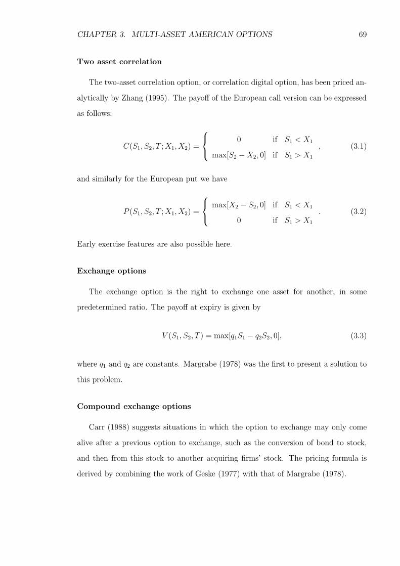
CHAPTER 3. MULTI-ASSET AMERICAN OPTIONS 69
Two asset correlation
The two-asset correlation option, or correlation digital option, has been priced an-
alytically by Zhang (1995). The payoff of the European call version can be expressed
as follows;
C(S1, S2, T ;X1, X2) =
0 if S1 < X1
max[S2 −X2, 0] if S1 > X1
, (3.1)
and similarly for the European put we have
P (S1, S2, T ;X1, X2) =
max[X2 − S2, 0] if S1 < X1
0 if S1 > X1
. (3.2)
Early exercise features are also possible here.
Exchange options
The exchange option is the right to exchange one asset for another, in some
predetermined ratio. The payoff at expiry is given by
V (S1, S2, T ) = max[q1S1 − q2S2, 0], (3.3)
where q1 and q2 are constants. Margrabe (1978) was the first to present a solution to
this problem.
Compound exchange options
Carr (1988) suggests situations in which the option to exchange may only come
alive after a previous option to exchange, such as the conversion of bond to stock,
and then from this stock to another acquiring firms’ stock. The pricing formula is
derived by combining the work of Geske (1977) with that of Margrabe (1978).

CHAPTER 3. MULTI-ASSET AMERICAN OPTIONS 70
Portfolio options
A portfolio option is an American (or European) style option and has a fixed
strike price. The payoff at expiry for the call is given by
max[(S1 + S2)−X, 0],
and for the put option it is
max[X − (S1 + S2), 0].
Basket options
The basket options have their values linked to the weighted sum over a number
of assets. They are very popular when hedging foreign exchange risk, since the value
of a basket is less than buying up individual options; they can typically be on a
large number of assets. Methods such as lattice or finite difference are not readily
able to handle a large number of dimensions, so the vast majority of the literature
on these options has focused on simulation. However, even simulation can struggle
when the dimensions is increased considerably, so the average price is often treated as
a stochastic process itself and priced using standard methods, with some error term
to account for the multi-dimensionality.
3.1 Literature
The exchange option was one of the first multi-dimensional options to be stud-
ied. Although options involving two underlyings, such as the convertible bond with
stochastic interest rates, had also been investigated, they do not have payoffs that
depend on both of the underlying factors. In his paper, Margrabe (1978) develops
the pricing equation for the European exchange option, as well as the American ex-
change option. The price is derived by setting up a hedged portfolio with zero return,
reducing the order of the problem to a single transformed asset BSM PDE, where
CHAPTER 3. MULTI-ASSET AMERICAN OPTIONS 71
the single transformed asset is the ratio of the two assets. From the multi-asset BSM
PDE, similarity solutions can derive the same pricing formula, as shown by Wilmott
(2001). Margrabe further shows that it is never optimal to exercise such an option
early.
Stulz (1982) studies the valuation of min-max options on two assets when the
strike prices on each of the assets are equal. This allows for some simplification and
the construction of an analytical formula for European options of this form, involving
the bivariate cumulative standard normal distribution. Johnson (1987) considers the
formula when the number of assets increases, again taking the ratio between assets
to be new transformed assets, so as to reduce the order of the problem; he obtains
relatively simple formula for the n-asset case, involving a multi-variate cumulative
standard normal distribution. Again however, the assumption of equal strike prices
is important in delivering these results. The solution for a dual strike option is
much harder to obtain. Boyle and Tse (1990) use an approach developed by Clark
(1961) to generate the first four moments of the maximum (minimum) of n jointly
normal random variables, to value calls or puts on the maximum or minimum of the
n assets. The results are compared to those of Johnson (1987) and give a reasonable
approximation. Broadie and Detemple (1997) investigate the early exercise region
on the American version of the maximum option, as well as some other options such
as the exchange option and capped exchange option. Villeneuve (1999) also presents
results on the existence and shape of the exercise region for options on two assets,
concentrating mainly on min/max options with a single strike price, and is able to
describe the shape of the exercise region in both the limit as maturity tends to infinity
(perpetual case), and in the limit as time tends to expiry. For the perpetual case,
Villeneuve (1999) shows that for the maximum of two puts (which he describes as
a put on the minimum of two assets), the optimal exercise boundary tends to the
critical value for the single asset, as the value of the other asset(s) tend to infinity.
In the limit as time tends to expiry, he presents results which complement those of
Broadie and Detemple (1997).
There have been numerous attempts to extend the binomial or trinomial tree

CHAPTER 3. MULTI-ASSET AMERICAN OPTIONS 72
to treat options including multiple assets. Boyle (1988) suggests an algorithm for a
lattice with two underlying assets, which Boyle et al. (1989) extend to the n-asset case.
In the algorithm suggested by Boyle (1988), the multi-factor model is an extension
of the trinomial tree, which, for a two-factor model, results in five possible states
at the next timestep, which leads to four equations in five unknowns, implying that
there is extra parameter that must be chosen carefully. The model used by Boyle
et al. (1989) circumvents this by abandoning the trinomial tree and allowing only
four possible states at the next time step, and hence is more easily extended to the
n-asset case. Kamrad and Ritchken (1991) improves the efficienccy of the multi-asset
lattice method, while Ho et al. (1995) extend the model to include a time-varying
variance-covariance structure.
An alternative method to pricing options on multiple assets was suggested by
Stapleton and Subrahmanyam (1984) when continuous trading in the relevant assets
is not possible. They generate the risk neutral valuation relationships under different
risk aversion preferences. Ho et al. (1997) extend the Geske and Johnson (1984)
approach to options on stocks with stochastic interest rates. The authors use a
multivariate binomial approximation of the underlying stock and zero-coupon prices
to price put options using up to three equally spaced exercise dates and Richardson
extrapolation. The effect of stochastic rates was significant for long- term options
with low asset volatility and high interest rates.
As noted earlier, the vast majority of the literature focuses on simulation to solve
multi-asset problems. Broadie and Glasserman (1997) obtain American option values
by Monte Carlo simulation, generating two algorithms, one with a high bias, which
takes advantage of future knowledge to calculate the optimal exercise boundary, and
one with a low bias, which does not, so both converge to the true price independently,
which creates a confidence interval. The computation time is linear in the number
of assets; however it is exponential in the number of exercise dates. Longstaff and
Schwartz (2001) propose a Monte-Carlo method, that is both linear in state variables
and linear in the number of exercise dates. The least-squares regression method, or
LSM, is just one method to use regression to calculate the value of early exercise.

CHAPTER 3. MULTI-ASSET AMERICAN OPTIONS 73
It is based on finding the value of the continuation function, or the expected future
payoff, at each time step. Such regression methods have been shown to give a upper
bound to the option value. Duck et al. (2005) exploit the manner in which the option
value converges to the true value in the LSM method to improve efficiency through
extrapolation. Andersen and Broadie (2004) use the work of Haugh and Kogan (2004)
to create an upper bound, and regression type analysis for the lower bound to improve
on the confidence intervals of Broadie and Glasserman (1997).
Another possible method is that of quadrature. Andricopoulos et al. (2007)
have extended their previous work on the single-asset quadrature (Andricopoulos
et al., 2003) to encompass multi-assets. Although the method suffers from the same
exponential increases in storage and calculations as do lattice methods (both trees
and finite-difference), the high speed of calculation enables reasonable results can be
obtained for several underlying assets.
In this chapter we attempt to improve on existing finite-difference methods for
pricing multi-asset options with a limited number of state variables (less than four).
Many of the options of interest on the market contain just two or three assets, while
many of the others can be reduced to a lower number of assets if the correlation be-
tween some of the assets is high. Here we choose to solve the problem by modifying the
PSOR algorithm (see chapter 2), since this is easily extended to two or more assets.
There is little literature in finance on the efficiency of the PSOR algorithm, however
Reisinger and Wittum (2004) apply multigrid methods to the American option prob-
lem, and investigate the most efficient block solving and projection to use. They find
that using blocks (see chapter 2 for a description of the block solver) of one dimension
less than the problem, i.e. point on a one-dimensional problem, one-dimensional on a
two-dimensional problem, or two-dimensional on a three-dimensional problem is the
most efficient. Villeneuve and Zanette (2002) adapt the alternating direction implicit
method (or ADI) to solve variational equalities, resulting in a computational scheme
that is around five times faster than a corresponding PSOR scheme. The PSOR
algorithm, with a fixed grid, will be able to price options with any number of payoffs,
such as those described above. However, with some knowledge about the solution
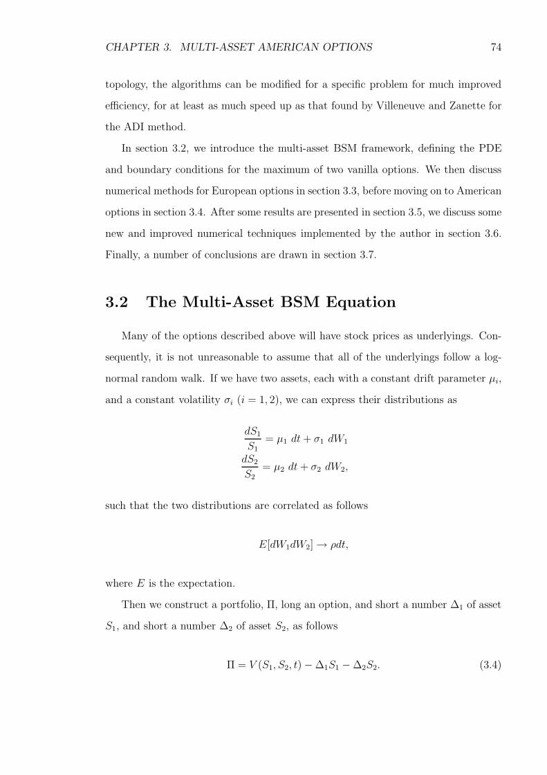
CHAPTER 3. MULTI-ASSET AMERICAN OPTIONS 74
topology, the algorithms can be modified for a specific problem for much improved
efficiency, for at least as much speed up as that found by Villeneuve and Zanette for
the ADI method.
In section 3.2, we introduce the multi-asset BSM framework, defining the PDE
and boundary conditions for the maximum of two vanilla options. We then discuss
numerical methods for European options in section 3.3, before moving on to American
options in section 3.4. After some results are presented in section 3.5, we discuss some
new and improved numerical techniques implemented by the author in section 3.6.
Finally, a number of conclusions are drawn in section 3.7.
3.2 The Multi-Asset BSM Equation
Many of the options described above will have stock prices as underlyings. Con-
sequently, it is not unreasonable to assume that all of the underlyings follow a log-
normal random walk. If we have two assets, each with a constant drift parameter µi,
and a constant volatility σi (i = 1, 2), we can express their distributions as
dS1
S1= µ1 dt+ σ1 dW1
dS2
S2= µ2 dt+ σ2 dW2,
such that the two distributions are correlated as follows
E[dW1dW2]→ ρdt,
where E is the expectation.
Then we construct a portfolio, Π, long an option, and short a number ∆1 of asset
S1, and short a number ∆2 of asset S2, as follows
Π = V (S1, S2, t)−∆1S1 −∆2S2. (3.4)
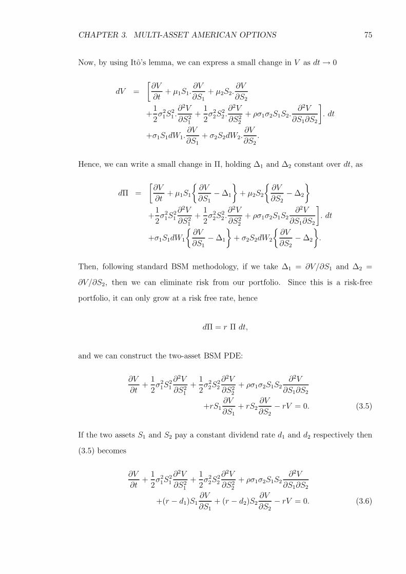
CHAPTER 3. MULTI-ASSET AMERICAN OPTIONS 75
Now, by using Ito’s lemma, we can express a small change in V as dt→ 0
dV =
[
∂V
∂t+ µ1S1.
∂V
∂S1
+ µ2S2.∂V
∂S2
+1
2σ2
1S21 .∂2V
∂S21
+1
2σ2
2S22 .∂2V
∂S22
+ ρσ1σ2S1S2.∂2V
∂S1∂S2
]
. dt
+σ1S1dW1.∂V
∂S1+ σ2S2dW2.
∂V
∂S2.
Hence, we can write a small change in Π, holding ∆1 and ∆2 constant over dt, as
dΠ =
[
∂V
∂t+ µ1S1
{
∂V
∂S1−∆1
}
+ µ2S2
{
∂V
∂S2−∆2
}
+1
2σ2
1S21
∂2V
∂S21
+1
2σ2
2S22 .∂2V
∂S22
+ ρσ1σ2S1S2∂2V
∂S1∂S2
]
. dt
+σ1S1dW1
{
∂V
∂S1
−∆1
}
+ σ2S2dW2
{
∂V
∂S2
−∆2
}
.
Then, following standard BSM methodology, if we take ∆1 = ∂V/∂S1 and ∆2 =
∂V/∂S2, then we can eliminate risk from our portfolio. Since this is a risk-free
portfolio, it can only grow at a risk free rate, hence
dΠ = r Π dt,
and we can construct the two-asset BSM PDE:
∂V
∂t+
1
2σ2
1S21
∂2V
∂S21
+1
2σ2
2S22
∂2V
∂S22
+ ρσ1σ2S1S2∂2V
∂S1∂S2
+rS1∂V
∂S1
+ rS2∂V
∂S2
− rV = 0. (3.5)
If the two assets S1 and S2 pay a constant dividend rate d1 and d2 respectively then
(3.5) becomes
∂V
∂t+
1
2σ2
1S21
∂2V
∂S21
+1
2σ2
2S22
∂2V
∂S22
+ ρσ1σ2S1S2∂2V
∂S1∂S2
+(r − d1)S1∂V
∂S1+ (r − d2)S2
∂V
∂S2− rV = 0. (3.6)

CHAPTER 3. MULTI-ASSET AMERICAN OPTIONS 76
By similar arguments, we can construct a general multi-asset BSM PDE, for n-
assets, Si, each paying a constant dividend rate di:
∂V
∂t+
n∑
i
n∑
j
1
2ρi,jσiσjSiSj
∂2V
∂Si∂Sj+
n∑
i
(r − di)Si∂V
∂Si− rV = 0. (3.7)
3.2.1 Maximum Options
Final conditions
The final condition for the maximum of two calls or puts is simple; at expiry
t = T , we can choose to either sell or buy either of the assets, at their respective
strike price. Then for the dual strike put at expiry we obtain
P (S1, S2, T ) = max[E1 − S1, E2 − S2, 0]. (3.8)
Similarly, for a dual strike call, we have
C(S1, S2, T ) = max[S1 − E1, S2 −E2, 0]. (3.9)
Boundary Conditions
The boundary conditions have to be imposed along lines rather than points (as
in the one-dimensional case), although sometimes the problem can be reduced to a
one-dimensional PDE on the boundary.
The conditions for the put are simple, so we will consider these first. Now, on
S1 = S2 = 0, then the option holder will receive max[E1, E2] at expiry, and so for
t < T
P (0, 0, t) = max[E1e−r(T−t), E2e
−r(T−t)]. (3.10)
On the S1 = 0 boundary, we now have an option depending on the S2 asset and t
only. If we set S1 = 0 into (3.6), then it will reduce the problem to the one-dimensional

CHAPTER 3. MULTI-ASSET AMERICAN OPTIONS 77
BSM equation in S2,
∂P
∂t+
1
2σ2
2S22
∂2P
∂S22
+ (r − d2)S2∂P
∂S2
− rP = 0, (3.11)
with the following conditions at expiry
P (0, S2, T ) = max[E2 − S2, E1]. (3.12)
Note here that if E1 ≥ E2 then P (0, S2, T ) = E1 and the boundary condition reduces
to
P (0, S2, t) = E1e−r(T−t). (3.13)
We can follow a similar argument for the S2 = 0 boundary.
We still require boundary conditions as each of the asset values become large.
This is straightforward when both assets are large, as the probability of the option to
exercise in either asset is small, so we have
P → 0 as both S1, S2 →∞. (3.14)
However, what if S1 → ∞, but S2 remains close to E2? Then, the probability of
ever exercising the option in S1 is practically zero, so a move up or down in S1 will
not affect the price of P . A similar argument follows in S2; from this we can set the
boundary condition to be
∂P (S1, S2, t)
∂S1
→ 0 as S1 →∞, (3.15)
∂P (S1, S2, t)
∂S2→ 0 as S2 →∞. (3.16)
Now we consider the corresponding conditions for a call. Almost identical to the
arguments presented for the put, the conditions at S1 = 0 and S2 = 0 are the solutions

CHAPTER 3. MULTI-ASSET AMERICAN OPTIONS 78
to the single-asset BSM equation. Therefore we arrive at the following conditions
C(S1 = 0, S2, t;E1, E2) = C∗(S2, t;E2, r, d2, σ2), (3.17)
C(S1, S2 = 0, t;E1, E2) = C∗(S1, t;E1, r, d1, σ1), (3.18)
where C∗ is the solution to the single asset BSM equation for a call option with final
conditions
C(S1 = 0, S2, t = T ;E1, E2) = max[0, S2 − E2], (3.19)
C(S1, S2 = 0, t = T ;E1, E2) = max[0, S1 −E1]. (3.20)
However, when we study the solution as S1 and S2 both become large, it is not as easy
to determine conditions as it was in the case for a put. A Neumann condition in either
direction will not be sufficient, since, in the region close to the line S1−E1 = S2−E2,
there is a discontinuity at payoff on the line S1 −E1 = S2 −E2 as S1 and S2 tend to
infinity, which persists for t < T in these limits.
Nevertheless, if we investigate the solution as S1 →∞ such that S1 >> S2, then
we can argue that any change in the price of asset S1, must lead to a corresponding
change in the option value, directly proportional to the change in S1, hence
∂V
∂S1
= 1. (3.21)
If we seek a solution of the form V (S1, S2, t) = S1−A(S2, t), as S1 →∞, substituting
into the BSM PDE (3.6), we have the following,
∂A
∂t+
1
2σ2
2S22 .∂2A
∂S22
+ (r − d2)S2∂A
∂S2− rA = 0, (3.22)
which is just the one asset BSM equation. A similar argument can be used for
S2 → ∞ such that S2 >> S1. This does not help us define a condition as S1 → ∞
and S2 → ∞ at the same rate, and we will attempt to reformulate this later in this
section. Next we show how it is possible to formulate a boundary condition for the

CHAPTER 3. MULTI-ASSET AMERICAN OPTIONS 79
simple single strike maximum of two calls.
Similarity Solution with E1 = E2
We need to employ a different method in order to obtain conditions for the call
as S1, S2 →∞ (simultaneously, at the same rate). The complexity of the problem is
reduced somewhat when we study the single strike option, with E1 = E2 = E. Now,
in the limit S1, S2 → ∞ the discontinuity around S1 = E and S2 = E becomes less
important1, so let us reduce the terminal condition to the simpler form,
V (S1, S2, T ) = max[S1 − E, S2 − E] .
The difference here is that the holder must exercise one of the two assets even if the
payout is negative. This option is close to the exchange option priced by Margrabe
(1978) and others. By using a similarity solution, note that we can solve exactly for
the simplified option over the entire domain with out the need to set S1 and S2 to
be large. This is not the case in the next subsection when we seek a solution where
E1 6= E2, a solution can only be found in the limit as the assets tend to infinity even
for the equivalent simplified option.
In order to solve the BSM equation with this terminal condition, we set
ξ =S2
S1.
and S = S1, then write,
V (S, ξ, t) = S H(ξ, t)−E, (3.23)
with H(ξ, T ) = max(1, ξ). Wilmott (2001) outlines a similar method for exchange
options, but this is slightly different because of the inclusion of the exercise price.
1When S1 and S2 are large, the holder of the maximum option will almost certainly receive apositive payoff, so the value of the option not to exercise will become insignificant.

CHAPTER 3. MULTI-ASSET AMERICAN OPTIONS 80
For the first derivatives we obtain
∂
∂S1
→ − ξS
∂
∂ξ+
∂
∂S∂
∂S2→ 1
S
∂
∂ξ(3.24)
and for the second derivatives we obtain
∂2
∂S21
→ ∂2
∂S2− 2ξ
S
∂2
∂S∂ξ+
2ξ
S2
∂
∂ξ+ξ2
S2
∂2
∂ξ2,
∂2
∂S1∂S2→ 1
S
∂2
∂ξ∂S− 1
S2
∂
∂ξ− ξ
S2
∂2
∂ξ2,
∂2
∂S2→ 1
S2
∂2
∂ξ2. (3.25)
Substituting the above into the BSM equation, we can express L2−BSM , the BSM
operator on two underlying assets, as
L2−BS =∂
∂t+
1
2σ2
1S2
{
∂2
∂S2− 2ξ
S
∂2
∂S∂ξ+
2ξ
S2
∂
∂ξ+ξ2
S2
∂2
∂ξ2
}
+1
2σ2
2S22
{
1
S2
∂2
∂ξ2
}
+ ρσ1σ2SS2
{
1
S
∂2
∂ξ∂S− 1
S2
∂
∂ξ− ξ
S2
∂2
∂ξ2
}
+(r − d1)S
{
− ξ
S
∂
∂ξ+
∂
∂S
}
+ (r − d2)S2
{
1
S
∂
∂ξ
}
− r. (3.26)
Therefore we must calculate L2−BS{V } = 0, from which we obtain the following
equation for H ,
∂H
∂t+
1
2σ2
1
{
ξ2∂2H
∂ξ2
}
+1
2σ2
2ξ2
{
∂2H
∂ξ2
}
+ ρσ1σ2ξ
{
− ξ ∂2H
∂ξ2
}
+(r − d1)
{
− ξ ∂H∂ξ
+H
}
+ (r − d2)ξ
{
∂H
∂ξ
}
− r(H − E
S) = 0.
On rearrangement this gives
∂H
∂t+ [
1
2σ2
1 − ρσ1σ2 +1
2σ2
2]ξ2∂
2H
∂ξ2+ [d1 − d2]ξ
∂H
∂ξ− d1H = −rE
S. (3.27)
We notice that on the left hand side, the equation in H is in fact just the BSM

CHAPTER 3. MULTI-ASSET AMERICAN OPTIONS 81
equation with ξ as the underlying asset, and −rE/S forming a constant coupon-like
term on the right-hand-side. As stated earlier, apart from justification to form the
final conditions, we have made no assumptions that S1 and S2 are large. Then we
can express (3.27) as
∂H
∂t+
1
2σ2ξ2∂
2H
∂ξ2+ (r − d)ξ ∂H
∂ξ− rH = K(S).
We have a function of ξ and t on the left hand side, and S on the right hand side,
hence a separable solution is appropriate. We can set each side of the equation equal
to a constant and then solve the resulting two equations independently, thus
LBS
{
H(ξ, t; σ, r, d)
}
= c (3.28)
K(S) = c , (3.29)
with σ =√
σ21 − 2ρσ1σ2 + σ2
2 , r = d1, d = d2 and c the separation constant. Then for
a particular value of S1, we can find c, and then we need only solve a simple BSM
equation to find the value at the boundary. We can easily interchange S1 for S2 to
obtain the same equation for a particular value of S2, with ξ = S1/S2.
General boundary condition with E1 6= E2
In the previous section the boundary condition for the single strike call option is
found relatively easily by a similarity solution, however for the dual strike option the
terms do not drop out so easily, and we must take an asymptotic approximation in
order to accurately find the boundary condition. Again, set the final condition on
the option be
V (S1, S2, T ) = max[S1 −E1, S2 − E2] ,
as we look for a solution for large S1 and S2. Then the appropriate substitutions will
be
ξ =S2 −E2
S1 −E1, S = S1 −E1 .

CHAPTER 3. MULTI-ASSET AMERICAN OPTIONS 82
and the option value can be written in the transformed coordinates as
V (S, ξ, t) = S H(ξ, t) ,
where H(ξ, T ) = max(1, ξ). Then under this transformation the derivatives will
remain the same as that calculated in the previous section (3.24) and (3.25), so after
substitution into the BSM operator, we obtain
L2−BS =∂
∂t+
1
2σ2
1(S + E1)2
{
∂2
∂S2− 2ξ
S
∂2
∂S∂ξ+
2ξ
S2
∂
∂ξ+ξ2
S2
∂2
∂ξ2
}
+1
2σ2
2S22
{
1
S2
∂2
∂ξ2
}
+ ρσ1σ2(S + E1)S2
{
1
S
∂2
∂ξ∂S− 1
S2
∂
∂ξ− ξ
S2
∂2
∂ξ2
}
+(r − d1)(S + E1)
{
− ξ
S
∂
∂ξ+
∂
∂S
}
+ (r − d2)S2
{
1
S
∂
∂ξ
}
− r. (3.30)
Next we apply the transformed BSM operator to V (S, ξ, t) to obtain
∂H
∂t+
1
2σ2
1
{
1 +2E1
S+E2
1
S2
}
ξ2∂2H
∂ξ2+
1
2σ2
2
{
ξ2 +2E2
S− E2
2
S2
}
∂2H
∂ξ2
−ρσ1σ2ξ
{
ξ + ξE1
S+E2
S+E1E2
S
}
∂2H
∂ξ2
+(r − d1)
{
1 +E1
S
}{
− ξ ∂H∂ξ
+H
}
+ (r − d2)
{
ξ +E2
S
}
∂H
∂ξ− rH = 0.
It is clear here that the solution is not separable, and we cannot solve the reduced
problem. Instead, let S →∞, and so to first order in S we have
∂H
∂t+
[
1
2σ2
1 − ρσ1σ2 +1
2σ2
2
]
ξ2∂2H
∂ξ2+ (d1 − d2)ξ
∂H
∂ξ+ (r − d2)ξ = 0 (3.31)
3.3 Numerical methods for the European Option
After discretisation we have a choice between using a direct solver or SOR solvers.
In one dimension the direct solver is always better than iterative methods, with in-
version of the matrix very simple using LU decomposition or Gaussian elimination.

CHAPTER 3. MULTI-ASSET AMERICAN OPTIONS 83
In two or more dimensions, the direct solver is advantageous when the rate of con-
vergence for the iterative solvers is sufficiently slow. However, the direct solver is
now much more difficult to code (it involves inverting a large matrix), although the
sparseness of the matrix may be exploited in some way, such as using a Big-Banded
Solver (BBS) or other sparse solvers from the NAG (or other) libraries (the sparse
solvers do involve iteration, so strictly should be classed as iterative solvers). There
are many situations, however, when the rate of convergence is very slow for the it-
erative solvers, such as if the volatility is high and the timesteps are large. Using
the Crank-Nicolson scheme allows the use of large timesteps due to the unconditional
stability imposed by the scheme.
The SOR method has long been known to perform better in higher dimensions
when the solution space is partitioned into blocks, which can be solved directly. These
blocks are typically a set of nodes encompassing a single line, plane or cube, depending
on the dimensionality of the problem. The errors can be bounded over the solution
space much more efficiently than when point SOR is used. For a two-dimensional
problem, we compare the direct solver with line or point SOR iteration in table 3.1.
Let us consider the two-asset case first. According to the Crank-Nicolson scheme
(Smith, 1985), the discretised equations may be written as
αi,juk+1i−1,j + (1/∆τ + βi,j)u
k+1i,j + γi,ju
k+1i+1,j + δi,ju
k+1i,j−1 + ǫi,ju
k+1i,j+1
+µi,j(uk+1i−1,j−1 − uk+1
i+1,j−1 − uk+1i−1,j+1 + uk+1
i+1,j+1) = Zki,j, (3.32)
where uki,j = V (i∆S1, j∆S2, k∆τ). Then in matrix form, this set of equations can be
expressed as
Auk+1 = bk, (3.33)
where uk+1 is the solution vector. The matrix A is sparse, typically only containing
less than 15 nonzero diagonal rows, depending on the boundary conditions. The
diagonal rows are grouped into three bands, separated by either n or m zero diagonal
rows, where n and m are the number of nodes in each direction. The way in which
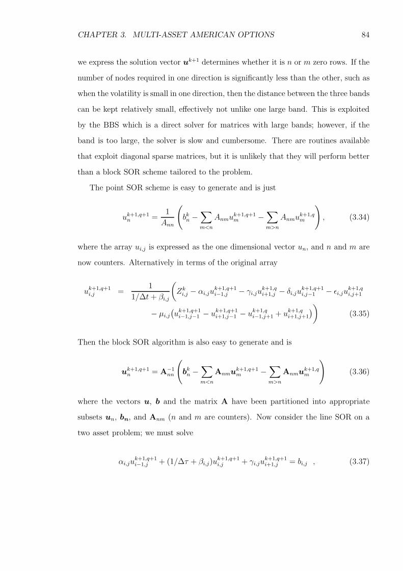
CHAPTER 3. MULTI-ASSET AMERICAN OPTIONS 84
we express the solution vector uk+1 determines whether it is n or m zero rows. If the
number of nodes required in one direction is significantly less than the other, such as
when the volatility is small in one direction, then the distance between the three bands
can be kept relatively small, effectively not unlike one large band. This is exploited
by the BBS which is a direct solver for matrices with large bands; however, if the
band is too large, the solver is slow and cumbersome. There are routines available
that exploit diagonal sparse matrices, but it is unlikely that they will perform better
than a block SOR scheme tailored to the problem.
The point SOR scheme is easy to generate and is just
uk+1,q+1n =
1
Ann
(
bkn −∑
m<n
Anmuk+1,q+1m −
∑
m>n
Anmuk+1,qm
)
, (3.34)
where the array ui,j is expressed as the one dimensional vector un, and n and m are
now counters. Alternatively in terms of the original array
uk+1,q+1i,j =
1
1/∆t+ βi,j
(
Zki,j − αi,ju
k+1,q+1i−1,j − γi,ju
k+1,qi+1,j − δi,juk+1,q+1
i,j−1 − ǫi,juk+1,qi,j+1
− µi,j
(
uk+1,q+1i−1,j−1 − uk+1,q+1
i+1,j−1 − uk+1,qi−1,j+1 + uk+1,q
i+1,j+1
)
)
(3.35)
Then the block SOR algorithm is also easy to generate and is
uk+1,q+1n = A−1
nn
(
bkn −
∑
m<n
Anmuk+1,q+1m −
∑
m>n
Anmuk+1,qm
)
(3.36)
where the vectors u, b and the matrix A have been partitioned into appropriate
subsets un, bn, and Anm (n and m are counters). Now consider the line SOR on a
two asset problem; we must solve
αi,juk+1,q+1i−1,j + (1/∆τ + βi,j)u
k+1,q+1i,j + γi,ju
k+1,q+1i+1,j = bi,j , (3.37)

CHAPTER 3. MULTI-ASSET AMERICAN OPTIONS 85
0 5
10 15
20 0 5
10 15
20
0
2.5
5
V (S1, S2, t)
S1 S2
(a) Put
0 5
10 15
20 0 5
10 15
20
0
2.5
5
7.5
10
12.5
V (S1, S2, t)
S1 S2
(b) Call
Figure 3.1The minimum of two vanilla options.
over 0 ≤ i ≤ N where
bi,j = Zki,j − δi,juk+1,q+1
i,j−1 − ǫi,juk+1,qi,j+1
−µi,j(uk+1,q+1i−1,j−1 − uk+1,q+1
i+1,j−1 − uk+1,qi−1,j+1 + uk+1,q
i+1,j+1). (3.38)
The value of j is held constant until all nodes in i have been found, using a direct
solver such as LU decomposition. Then we can move through all values of j to solve
over the entire space. The constant value can be interchanged in i and j so that the
errors may be bounded.
3.3.1 Results
Figures 3.1-3.4 show the values of various different European options on two assets.
All four figures correspond to E1 = 10, E2 = 5, d1 = d2 = ρ = 0, σ1 = σ2 = 0.2, and
T = 0.5. Later, we will consider the solution to American options, but these graphs,
along with the schematics of the terminal exercise regions, can give an indication of
the positioning of the free boundary for the corresponding American option. This
may be exploited later in order to improve the PSOR algorithm. If we plot the
payoff function along with the European option value, we can find the regions in
which the European option is less than the exercise value. We may then assume that
the free boundary will be approximately of the same topology as the intersection of
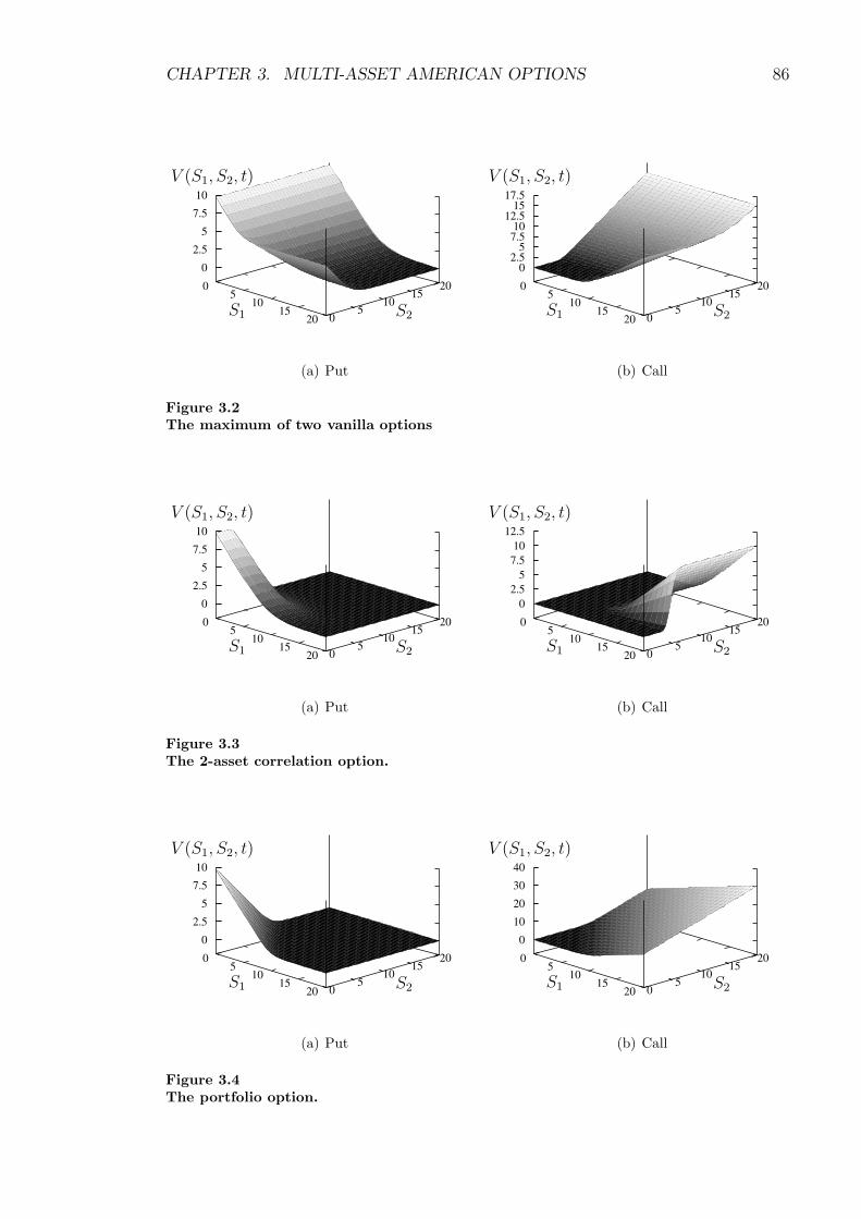
CHAPTER 3. MULTI-ASSET AMERICAN OPTIONS 86
0 5
10 15
20 0 5
10 15
20
0
2.5
5
7.5
10
V (S1, S2, t)
S1 S2
(a) Put
0 5
10 15
20 0 5
10 15
20
0
2.5
5
7.5
10
12.5
15
17.5
V (S1, S2, t)
S1 S2
(b) Call
Figure 3.2The maximum of two vanilla options
0 5
10 15
20 0 5
10 15
20
0
2.5
5
7.5
10
V (S1, S2, t)
S1 S2
(a) Put
0 5
10 15
20 0 5
10 15
20
0
2.5
5
7.5
10
12.5
V (S1, S2, t)
S1 S2
(b) Call
Figure 3.3The 2-asset correlation option.
0 5
10 15
20 0 5
10 15
20
0
2.5
5
7.5
10
V (S1, S2, t)
S1 S2
(a) Put
0 5
10 15
20 0 5
10 15
20
0
10
20
30
40
V (S1, S2, t)
S1 S2
(b) Call
Figure 3.4The portfolio option.
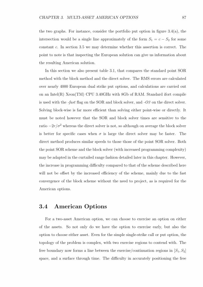
CHAPTER 3. MULTI-ASSET AMERICAN OPTIONS 87
the two graphs. For instance, consider the portfolio put option in figure 3.4(a), the
intersection would be a single line approximately of the form S1 = c − S2 for some
constant c. In section 3.5 we may determine whether this assertion is correct. The
point to note is that inspecting the European solution can give us information about
the resulting American solution.
In this section we also present table 3.1, that compares the standard point SOR
method with the block method and the direct solver. The RMS errors are calculated
over nearly 4000 European dual strike put options, and calculations are carried out
on an Intel(R) Xeon(TM) CPU 3.40GHz with 8Gb of RAM. Standard ifort compile
is used with the -fast flag on the SOR and block solver, and -O3 on the direct solver.
Solving block-wise is far more efficient than solving either point-wise or directly. It
must be noted however that the SOR and block solver times are sensitive to the
ratio −2r/σ2 whereas the direct solver is not, so although on average the block solver
is better for specific cases when σ is large the direct solver may be faster. The
direct method produces similar speeds to those those of the point SOR solver. Both
the point SOR scheme and the block solver (with increased programming complexity)
may be adapted in the curtailed range fashion detailed later in this chapter. However,
the increase in programming difficulty compared to that of the scheme described here
will not be offset by the increased efficiency of the scheme, mainly due to the fast
convergence of the block scheme without the need to project, as is required for the
American options.
3.4 American Options
For a two-asset American option, we can choose to exercise an option on either
of the assets. So not only do we have the option to exercise early, but also the
option to choose either asset. Even for the simple single-strike call or put option, the
topology of the problem is complex, with two exercise regions to contend with. The
free boundary now forms a line between the exercise/continuation regions in [S1, S2]
space, and a surface through time. The difficulty in accurately positioning the free
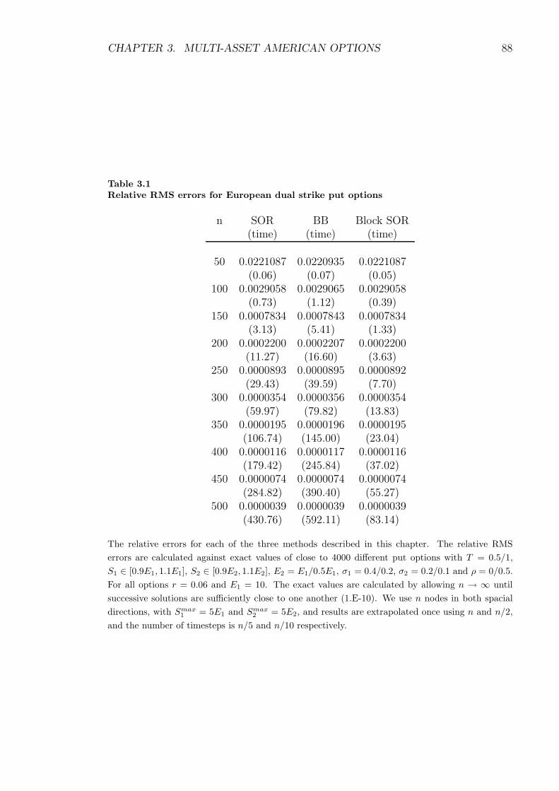
CHAPTER 3. MULTI-ASSET AMERICAN OPTIONS 88
Table 3.1Relative RMS errors for European dual strike put options
n SOR BB Block SOR(time) (time) (time)
50 0.0221087 0.0220935 0.0221087(0.06) (0.07) (0.05)
100 0.0029058 0.0029065 0.0029058(0.73) (1.12) (0.39)
150 0.0007834 0.0007843 0.0007834(3.13) (5.41) (1.33)
200 0.0002200 0.0002207 0.0002200(11.27) (16.60) (3.63)
250 0.0000893 0.0000895 0.0000892(29.43) (39.59) (7.70)
300 0.0000354 0.0000356 0.0000354(59.97) (79.82) (13.83)
350 0.0000195 0.0000196 0.0000195(106.74) (145.00) (23.04)
400 0.0000116 0.0000117 0.0000116(179.42) (245.84) (37.02)
450 0.0000074 0.0000074 0.0000074(284.82) (390.40) (55.27)
500 0.0000039 0.0000039 0.0000039(430.76) (592.11) (83.14)
The relative errors for each of the three methods described in this chapter. The relative RMS
errors are calculated against exact values of close to 4000 different put options with T = 0.5/1,
S1 ∈ [0.9E1, 1.1E1], S2 ∈ [0.9E2, 1.1E2], E2 = E1/0.5E1, σ1 = 0.4/0.2, σ2 = 0.2/0.1 and ρ = 0/0.5.
For all options r = 0.06 and E1 = 10. The exact values are calculated by allowing n → ∞ until
successive solutions are sufficiently close to one another (1.E-10). We use n nodes in both spacial
directions, with Smax1 = 5E1 and Smax
2 = 5E2, and results are extrapolated once using n and n/2,
and the number of timesteps is n/5 and n/10 respectively.
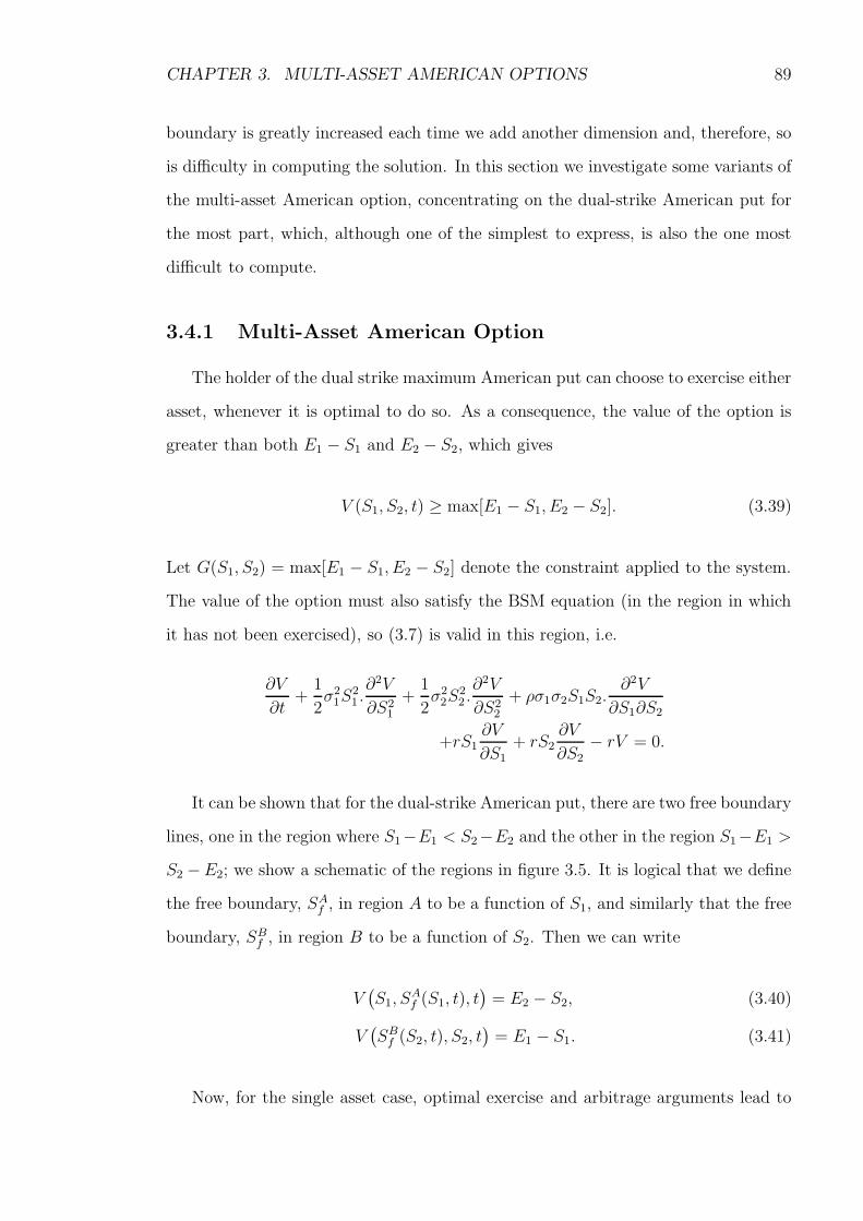
CHAPTER 3. MULTI-ASSET AMERICAN OPTIONS 89
boundary is greatly increased each time we add another dimension and, therefore, so
is difficulty in computing the solution. In this section we investigate some variants of
the multi-asset American option, concentrating on the dual-strike American put for
the most part, which, although one of the simplest to express, is also the one most
difficult to compute.
3.4.1 Multi-Asset American Option
The holder of the dual strike maximum American put can choose to exercise either
asset, whenever it is optimal to do so. As a consequence, the value of the option is
greater than both E1 − S1 and E2 − S2, which gives
V (S1, S2, t) ≥ max[E1 − S1, E2 − S2]. (3.39)
Let G(S1, S2) = max[E1 − S1, E2 − S2] denote the constraint applied to the system.
The value of the option must also satisfy the BSM equation (in the region in which
it has not been exercised), so (3.7) is valid in this region, i.e.
∂V
∂t+
1
2σ2
1S21 .∂2V
∂S21
+1
2σ2
2S22 .∂2V
∂S22
+ ρσ1σ2S1S2.∂2V
∂S1∂S2
+rS1∂V
∂S1
+ rS2∂V
∂S2
− rV = 0.
It can be shown that for the dual-strike American put, there are two free boundary
lines, one in the region where S1−E1 < S2−E2 and the other in the region S1−E1 >
S2 −E2; we show a schematic of the regions in figure 3.5. It is logical that we define
the free boundary, SAf , in region A to be a function of S1, and similarly that the free
boundary, SBf , in region B to be a function of S2. Then we can write
V(
S1, SAf (S1, t), t
)
= E2 − S2, (3.40)
V(
SBf (S2, t), S2, t
)
= E1 − S1. (3.41)
Now, for the single asset case, optimal exercise and arbitrage arguments lead to
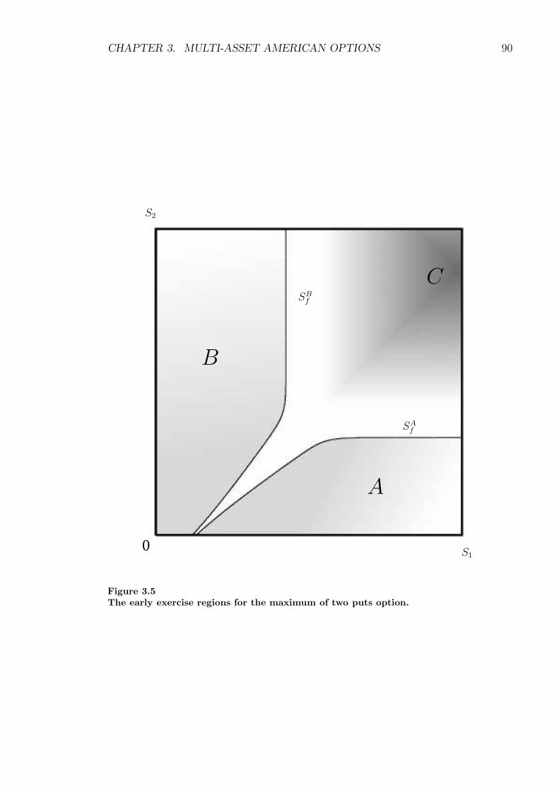
CHAPTER 3. MULTI-ASSET AMERICAN OPTIONS 90
0
A
B
C
S1
S2
SAf
SBf
Figure 3.5The early exercise regions for the maximum of two puts option.

CHAPTER 3. MULTI-ASSET AMERICAN OPTIONS 91
the smooth pasting condition for the American put at the optimal exercise boundary.
With similar arguments, the maximum American put option also has a smooth past-
ing condition, although we must enforce the continuity of ∆ in both of the assets.
This gives us four more constraints on the free boundary, namely
∂V
∂S1
(
S1, SAf (S1, t), t
)
= 0,
∂V
∂S2
(
S1, SAf (S1, t), t
)
= −1,
∂V
∂S1
(
SBf (S2, t), S2, t
)
= −1,
∂V
∂S2
(
SBf (S2, t), S2, t
)
= 0. (3.42)
These four constraints equate to two tangential derivative conditions. We can see
here that adding one more dimension has made it impractical to use a boundary-
fitted coordinate system such as that used to solve for the one-dimensional case in
chapter 2. It is possible to specify a mapping from the region in (S1, S2) space to
the unit square (S1, S2) using similar transformations to those used for the single
asset American put or call, although to implement such a scheme would rely on
the topology of the problem to be of appropriate form. Even then, the increased
complexity of the problem may reduce any possible benefits.
If we solve for a multi-strike option, with more than two assets, the complexity
of even the free boundary formulation will become tedious. It is sufficient to say
that the smooth pasting condition ensures that at each point on the free boundary,
all partial derivatives in Si must be equal to the corresponding derivative of the
constraint G at that point. This leads to the conclusion that the most appropriate
(finite-difference) methods to solve for an American option in multi-dimensions are
variational techniques, of which the PSOR scheme is one implementation. The PSOR
scheme applied to multi-asset option is described in the next section.

CHAPTER 3. MULTI-ASSET AMERICAN OPTIONS 92
3.4.2 PSOR on Multi-Asset Options
The PSOR method is easily extended to multi-asset options and because the
method is a fixed grid method, a solution can be obtained without detailed prior
knowledge of the number of distinct regions in solution space in which it is optimal
to exercise or not to exercise. We study the two asset problem in detail, which can
be generalised to the multi-asset case.
The problem is discretised in the usual manner
V (i ·∆S1, j ·∆S2, k ·∆t) = uki,j ,
G(i ·∆S1, j ·∆S2, k ·∆t) = gki,j ,
then we refer to (3.32) for the discrete approximation to the BSM PDE. Now let us
express (3.32) in matrix form. Let uk and gk denote the vectors
uk =
xk0,0
...
xkn,0
xk0,1
...
xkn,m
, gk =
gk0,0
...
gkn,0
gk0,1
...
gkn,m
.
We can then construct a matrix A and a vector bk such that we can rewrite (3.32)
as
Auk+1 = bk.
We can then express the problem in linear complementary form:
(
Auk+1 − bk
)
·(
uk+1 − gk+1
)
= 0. (3.43)
Now (3.43) is identical to (2.79), so we can adapt the SOR algorithm to obtain

CHAPTER 3. MULTI-ASSET AMERICAN OPTIONS 93
the projected SOR solver:
yk+1,q+1i,j =
1
1/∆t+ βi,j
(
Zki,j − αi,ju
k+1,q+1i−1,j − γi,ju
k+1,qi+1,j − δi,juk+1,q+1
i,j−1 − ǫi,juk+1,qi,j+1
−µi,j
(
uk+1,q+1i−1,j−1 − uk+1,q+1
i+1,j−1 − uk+1,qi−1,j+1 + uk+1,q
i+1,j+1
)
)
, (3.44)
uk+1,q+1i,j = max
[
uk+1,qi,j + ω(yk+1,q+1
i,j − uk+1,qi,j ), gk+1
i,j
]
. (3.45)
As we iterate over these two equations we will have a consistent solution that satisfies
either Auk+1 = bk or uk+1 = gk+1.
In the single-asset case (chapter 2), the boundary conditions were explicitly de-
fined. In the two-asset case however, we must solve a PDE along the boundary
lines using the PSOR scheme in order to satisfy the appropriate constraints. We
use the boundary conditions defined by equations (3.11), (3.15), and (3.16) to form
Auk+1 = bk for a put, and (3.17), (3.18), (3.28) and (3.29) for the call.
3.5 Results
In the following section we discuss solutions to the American problem, and the
specific properties which allow us to enhance the numerical techniques used to solve
the problem. The results are represented in both graphical and tabular form.
3.5.1 The Early Exercise Region
The early exercise regions for various different options are shown in figures 3.6-
3.8. The free boundary is found as a result of the algorithm used to solve the option
(cf section 3.6.3) defined as the outer-most node at which the option is exercised.
Figure 3.6 shows the most common class of put to be investigated, the maximum
of two options on a single strike price, or a put/call on the minimum of two assets.
The shape and magnitude of the results agree with those detailed by Broadie and
Detemple (1997). We note the terminal condition of the free boundary, either by
inspection, or by asymptotic analysis. For the put (figure 3.6(a)), the condition is

CHAPTER 3. MULTI-ASSET AMERICAN OPTIONS 94
given by;
SAf (S1, T ) = max
[
0,min
[
S1, E,r E
d2
]]
(3.46)
SBf (S2, T ) = max
[
0,min
[
S2, E,r E
d1
]]
, (3.47)
and for the call (figure 3.6(b)) it is
SBf (S1, T ) = max
[
S1, E,r E
d2
]
(3.48)
SAf (S2, T ) = max
[
S2, E,r E
d1
]
. (3.49)
Both of these conditions are fairly straightforward to derive, by discarding the second
order derivatives and looking at the first order solutions. Here we have defined the
line S1 = S2 to be a free boundary line at expiry, when clearly the option should
be exercised on this line. However, we define the free boundary at expiry to be the
value in the limit as time tends to expiry. The argument as to why the holder never
exercises when S1 = S2 until expiry is simple. Suppose that S1 = S2, and the holder
exercises asset S2, and then there is movement up or down in S1, the holder would
be better off to have waited to see if it was beneficial to exercise asset S1. Then it is
the option to choose which asset to exercise which causes the limit at expiry of the
free boundary to be S1 = S2.
The early exercise region is shown over a range of times, and we can see how
the region develops. For the maximum put, we can see that when S1 is large, and
the likelihood of the option being exercised in the S1 asset is therefore small, the
free boundary SAf behaves as that for the single asset case. In figure 3.6(a), the
chosen values of σ1 and σ2, 0.4 and 0.2 respectively, are significantly different, as
SAf (S1 = 20) ≈ 8.25 and SB
f (S2 = 20) ≈ 6.4 shows. However, for S1 < 10 and S2 < 10
the free boundary appears to be approximately symmetric around the line S1 = S2,
suggesting that it is the combination of the two volatilities and their correlation that
drives the pricing in this region. The rate at which the free boundary moves in this
region (S1 ≈ S2) with time is also far faster than the boundary moves for large S1 or
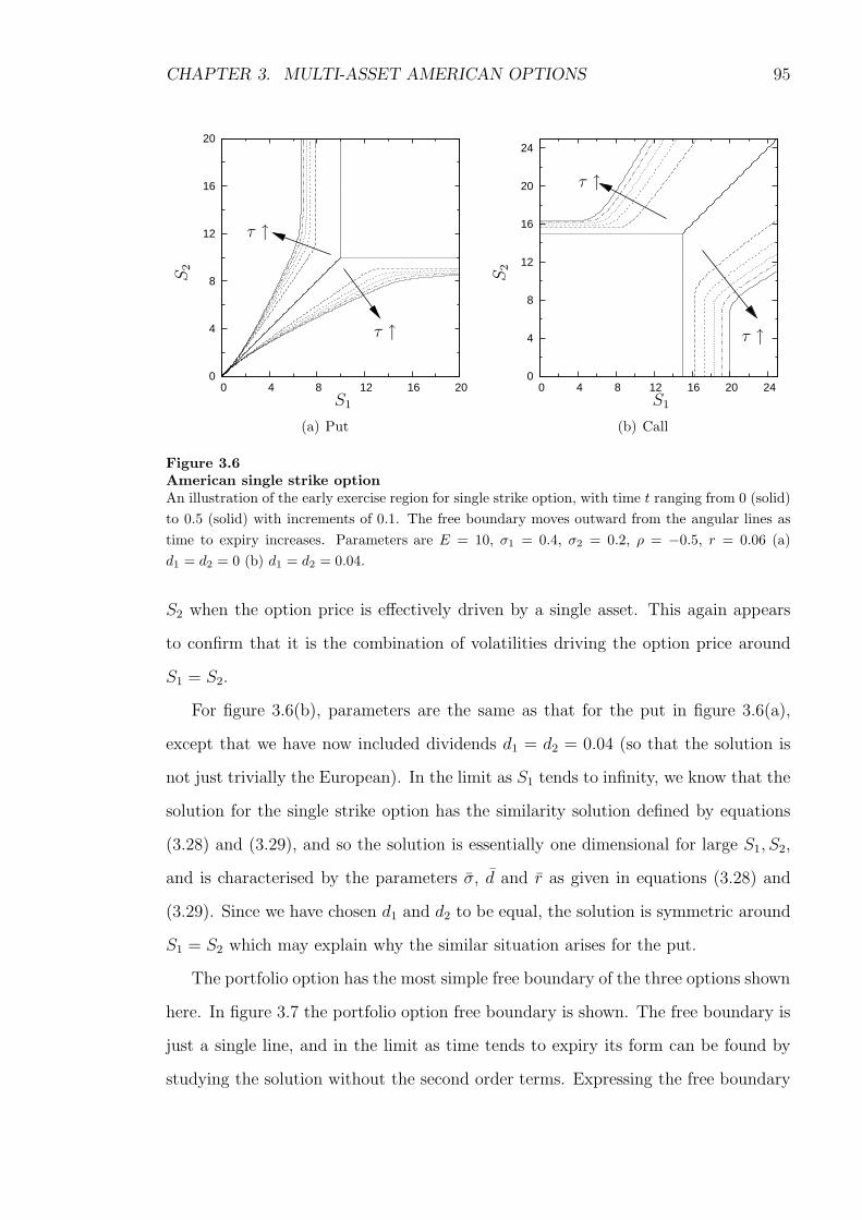
CHAPTER 3. MULTI-ASSET AMERICAN OPTIONS 95
0
4
8
12
16
20
0 4 8 12 16 20
τ ↑
τ ↑
S1
S2
(a) Put
0
4
8
12
16
20
24
0 4 8 12 16 20 24
τ ↑
τ ↑
S1
S2
(b) Call
Figure 3.6American single strike optionAn illustration of the early exercise region for single strike option, with time t ranging from 0 (solid)
to 0.5 (solid) with increments of 0.1. The free boundary moves outward from the angular lines as
time to expiry increases. Parameters are E = 10, σ1 = 0.4, σ2 = 0.2, ρ = −0.5, r = 0.06 (a)
d1 = d2 = 0 (b) d1 = d2 = 0.04.
S2 when the option price is effectively driven by a single asset. This again appears
to confirm that it is the combination of volatilities driving the option price around
S1 = S2.
For figure 3.6(b), parameters are the same as that for the put in figure 3.6(a),
except that we have now included dividends d1 = d2 = 0.04 (so that the solution is
not just trivially the European). In the limit as S1 tends to infinity, we know that the
solution for the single strike option has the similarity solution defined by equations
(3.28) and (3.29), and so the solution is essentially one dimensional for large S1, S2,
and is characterised by the parameters σ, d and r as given in equations (3.28) and
(3.29). Since we have chosen d1 and d2 to be equal, the solution is symmetric around
S1 = S2 which may explain why the similar situation arises for the put.
The portfolio option has the most simple free boundary of the three options shown
here. In figure 3.7 the portfolio option free boundary is shown. The free boundary is
just a single line, and in the limit as time tends to expiry its form can be found by
studying the solution without the second order terms. Expressing the free boundary
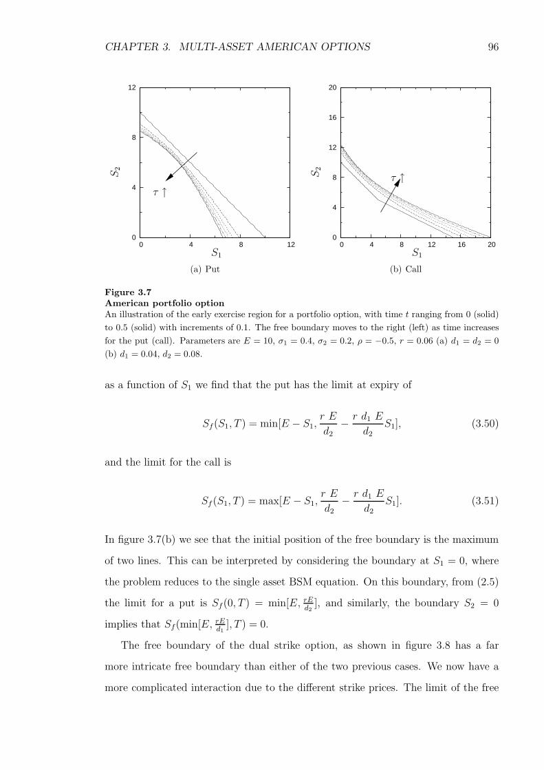
CHAPTER 3. MULTI-ASSET AMERICAN OPTIONS 96
0
4
8
12
0 4 8 12
τ ↑
S1
S2
(a) Put
0
4
8
12
16
20
0 4 8 12 16 20
τ ↑
S1
S2
(b) Call
Figure 3.7American portfolio optionAn illustration of the early exercise region for a portfolio option, with time t ranging from 0 (solid)
to 0.5 (solid) with increments of 0.1. The free boundary moves to the right (left) as time increases
for the put (call). Parameters are E = 10, σ1 = 0.4, σ2 = 0.2, ρ = −0.5, r = 0.06 (a) d1 = d2 = 0
(b) d1 = 0.04, d2 = 0.08.
as a function of S1 we find that the put has the limit at expiry of
Sf(S1, T ) = min[E − S1,r E
d2
− r d1 E
d2
S1], (3.50)
and the limit for the call is
Sf (S1, T ) = max[E − S1,r E
d2
− r d1 E
d2
S1]. (3.51)
In figure 3.7(b) we see that the initial position of the free boundary is the maximum
of two lines. This can be interpreted by considering the boundary at S1 = 0, where
the problem reduces to the single asset BSM equation. On this boundary, from (2.5)
the limit for a put is Sf(0, T ) = min[E, rEd2
], and similarly, the boundary S2 = 0
implies that Sf(min[E, rEd1
], T ) = 0.
The free boundary of the dual strike option, as shown in figure 3.8 has a far
more intricate free boundary than either of the two previous cases. We now have a
more complicated interaction due to the different strike prices. The limit of the free

CHAPTER 3. MULTI-ASSET AMERICAN OPTIONS 97
0
4
8
12
16
20
0 4 8 12 16 20
τ ↑
τ ↑
S1
S2
(a) Put
0
4
8
12
16
20
24
0 4 8 12 16 20 24
τ ↑
τ ↑
S1
S2
(b) Call
Figure 3.8American dual strike optionAn illustration of the early exercise region for dual strike option, with time t ranging from 0 (solid)
to 0.5 (solid) with increments of 0.1. The free boundary moves outward from the angular lines as
time to expiry increases. Parameters are E1 = 10, E2 = 5, σ1 = 0.4, σ2 = 0.2, ρ = −0.5, r = 0.06
(a) d1 = d2 = 0 (b) d1 = 0.04, d2 = 0.04.
boundary as time tends to expiry is found to be
SAf (S1, T ) = max
[
0,min
[
S1 −E1 + E2, E2,r E2
d2
]]
(3.52)
SBf (S2, T ) = max
[
0,min
[
S2 −E2 + E2, E1,r E1
d1
]]
, (3.53)
for the put (figure 3.8(a)) and for the call (figure 3.8(b)) it is
SBf (S1, T ) = max
[
S1 − E1 + E2, E2,r E2
d2
]
(3.54)
SAf (S2, T ) = max
[
S2 − E2 + E2, E1,r E1
d1
]
. (3.55)
Although the shape of the boundaries is similar to the single strike option (fig-
ure 3.6), the boundary is no longer symmetric around the line S1 = S2 − E2 + E1,
and is skewed to one side.

CHAPTER 3. MULTI-ASSET AMERICAN OPTIONS 98
3.6 Enhanced Numerical Techniques
Even with the rapid growth of computer power, the numerical solution to PDEs
with multi dimensions can still be a problem. In order to maintain accuracy as we
increase the number of dimensions, the number of nodes over which we must solve
grows exponentially. The numerical techniques developed for the single-dimension
case are not as robust/efficient in multiple dimensions.
3.6.1 Optimising the relaxation parameter ω
Work on optimising the over-relaxation parameter ω has been carried out by Cryer
(1971), who has shown that the optimum value of ω for the linear complementarity
PSOR scheme is always slightly less than that for the corresponding linear SOR
scheme. For the one-dimensional case, by running an optimising algorithm with the
solver, the optimum value of ω was found to be between 1.6 and 1.8. When the scheme
was modified to involve a block solver, in the APSOR (see later section 3.6.3), the
optimum value was also found to be around 1.6 to 1.8. The value is highly dependent
on the value of σ1 and σ2 and also the size of the time-steps.
3.6.2 Simple Banding
Andricopoulos et al. (2004) show that when solving using trees, the number of
nodes over which you must solve can be reduced according to the probability of exer-
cising at a particular node, and the probability of reaching that node, starting from
the initial node. Inspection of the solution for the American put, shown diagram-
matically in figure 3.5, indicates that there are significant regions in state space over
which it is unnecessary solve. In regions A and B the option is exercised, and in
region C the option is worthless since the probability of it ever being exercised is so
small.
If we are to solve the PDE, discarding regions where the option is exercised or
worthless, then we must fully understand the topology of the problem, ensuring that
these discarded regions play no role at any time. Region C is calculated following
CHAPTER 3. MULTI-ASSET AMERICAN OPTIONS 99
Andricopolous et al. (2002),
Smax1 = E1 · e−r(T−t)+ξσ1
√T−t (3.56)
Smax2 = E2 · e−r(T−t)+ξσ1
√T−t. (3.57)
Now let us consider regions A and B for the two-asset American put. For a single
asset put, it is simple to find a minimum for the free boundary. We simply look at
the perpetual option for which we have an analytical solution. Now, we know
P (S, T − t1) > P (S, T − t2) for t1 < t2, (3.58)
where P (S, t) is the single asset American put option. This statement says that the
option price is monotonically increasing as we move backwards in time, a detailed
description as to why this is so can be found later in chapter 7, where other such
rational pricing criteria are discussed. Since the option price is always increasing as we
move backwards in time, then the free boundary must be monotonically decreasing,
or
Sf (T − t1) < Sf(T − t2) for t1 < t2, (3.59)
where Sf(t) is the free boundary. In the limit as time to maturity becomes large we
can write
lim(T−t)→∞
P (S, t) = P ∗(S),
lim(T−t)→∞
Sf (t) = S∗f ,
where P ∗, S∗f is the perpetual option and the corresponding free boundary respec-
tively, since S∗f is a minimum for Sf(t). Now, if V (S1, S2, t) is the price of the dual
strike American option, as S1 →∞ the boundary condition that ∂∂S1
= 0 implies that
V (S1, S2, t)→ P (S2, t;E2, σ2, r, d2), (3.60)
CHAPTER 3. MULTI-ASSET AMERICAN OPTIONS 100
where P (S2, t) is the solution to the single asset BSM equation with the given pa-
rameters. From our reasoning above it is clear that
limS1→∞
SAf (S1, t) = Sf(t) (3.61)
where Sf (t) is the free boundary for P (S2, t).
Let the region for which we will discard, inside A, (cf figure 3.5) have the boundary
CA(S1). Then we require
CA(S1) ≤ lim(T−t)→∞
SAf (S1). (3.62)
If we could solve the perpetual case for two-assets, then
CA(S1) = lim(T−t)→∞
SAf (S1),
CB(S2) = lim(T−t)→∞
SBf (S2),
and our two regions are well defined. The author is unaware of any analytical solution
for the two-asset problem, however, there is an analytical solution to the single-asset
perpetual American option with two free boundaries. The next section describes how,
in a somewhat heuristic approach, the solution to such a problem can be exploited
to estimate the perpetual location of the free boundary.
A perpetual option with two free boundaries
In order to reduce the complexity of the problem, we consider a slice (with constant
S2) of the solution in the region S2 < E2. Let such a slice be defined where E = E2−S2
is a constant, where V is now just a function of S1, then the final condition of this
option is
V (S1, t = T ) = max[E, E1 − S1]. (3.63)
Then since we ignore the effects of variations in S2, the problem will reduce to the
one-dimensional case, now with two free boundaries, and a smooth pasting condition
on each. The motivation for investigating such an option is to give an estimation of

CHAPTER 3. MULTI-ASSET AMERICAN OPTIONS 101
the lower bound for the free boundary, and so we are only interested in the limit as
time tends to infinity, i.e. the perpetual option, as this is the when the free boundary
is expected to reach its minimum. To compensate for not considering derivatives
in the S2 direction, let us introduce a new volatility, that takes into account the
volatility in both directions,
σ =√
σ1 − 2ρσ1σ2 + σ2.
This volatility is similar to (3.27) derived earlier when a similarity solution is used
to solve in the limit as S1 →∞. For this option, an analytical solution exists for the
steady state solution, or the perpetual option, which we will now derive.
By seeking a solution of the Euler type
V (S) = ASα, (3.64)
we can insert this into the one dimensional BSM (less the time derivative) with our
modified volatility
1
2σ2S2
1
∂V
∂S21
+ (r − d1)S1∂V
∂S1− rV = 0, (3.65)
we arrive at a solution of the form
V (S) = ASα− +BSα+ , (3.66)
where α+ and α− denote the positive and negative roots respectively of the quadratic
equation
1
2σ2α(α− 1) + (r − d1)α + r = 0. (3.67)
We now require the boundary conditions at S1 = Sl, the lower boundary, and
S1 = Su, the upper boundary. Since we exercise at the free boundary, we have
V (S1 = Sl) = E1 − S1, (3.68)
V (S1 = Su) = E. (3.69)

CHAPTER 3. MULTI-ASSET AMERICAN OPTIONS 102
From the smooth pasting conditions we obtain
∂V
∂S1
(S1 = Sl) = −1, (3.70)
∂V
∂S1
(S1 = Su) = 0. (3.71)
Now, (3.69) implies that
ASα−
u +BSα+u = E,
B = (E −A · Sα−
u )S−α+u . (3.72)
and so
A =Eα+
α+Sα−
u − α−Sα−
u. (3.73)
So if we substitute (3.72) and (3.73) into (3.68) and (3.70) we obtain
Eα+
α+Sα−
u − α−Sα−
uS
α−
l +
(
E − Eα+
α+Sα−
u − α−Sα−
uSα
−
u
)
S−α+u S
α+
l
= E1 − Sl, (3.74)
Eα+
α+Sα−
u − α−Sα−
uα−S
α−−1
l +
(
E − Eα+
α+Sα−
u − α−Sα−
uSα
−
u
)
S−α+u α+S
α+−1l
= −1. (3.75)
After some algebra on (3.74) and (3.75) we find
E · α+
α+ − α−· S
α−
l
Sα−
u− E · α−
α+ − α−· S
α+
l
Sα+u
= E1 − Sl, (3.76)
E · α+α−
α+ − α−· S
α−
l
Sα−
u− E · α−α+
α+ − α−· S
α+
l
Sα+u
= −Sl. (3.77)

CHAPTER 3. MULTI-ASSET AMERICAN OPTIONS 103
These equations lead to the conclusion that
(α+ − α+α−)E
α+ − α−· S
α−
l
Sα−
u− (α− − α+α−)
E
α+ − α−· S
α+
l
Sα+u
= E1,
Sα−
l
Sα−
u− α− − α+α−
α+ − α+α−· S
α+
l
Sα+u
=E1(α+ − α−)
E(α+ − α+α−). (3.78)
If we assume that dividends d1 are zero, then α+ = 1 and α− = 2rσ2 , the equation may
be solved explicitly
Sl
Su=
(
E1
E
)1
α−
, (3.79)
and therefore
Sl =α−E
1− α−
{
(
E1
E
)1
α−
− E1
E
}
(3.80)
Su =α−E1
1− α−
E
E1−(
E
E1
)1
α−
. (3.81)
and as a consequence the solution to the problem (without dividends) is
V (S1) =E
Sα−
u − α−Sα−
u· Sα
−
1 −α−E
Su − α−Su
· S1 . (3.82)
In figure 3.9 we plot the perpetual free boundary, along with our estimate, gleaned
using the analysis above. The estimate is made by using the appropriate value for
E, given the value of S2. We note here that the analysis assumed the dividend value
to be zero, in order to gain an analytical boundary. Even with dividends included,
an appropriate increase or decrease in the value of σ and r should be able to take
any increase (decrease) in the free boundary into account. The estimate appears to
follow closely the path of the actual barrier, and importantly is always inside the
region of exercise where required. Using this boundary, the computation time can be
decreased by a large factor, as shown in table 3.2, especially when the values of σ1
and σ2 are small.

CHAPTER 3. MULTI-ASSET AMERICAN OPTIONS 104
0
4
8
12
16
20
0 4 8 12 16 20
S1
S2
(a) ρ = 0.75
0
4
8
12
16
20
0 4 8 12 16 20
S1
S2
(b) ρ = −0.75
Figure 3.9Simple banded estimateAn illustration of the early exercise region for single-strike perpetual put option (solid) along with
our estimates Sl (dotted) and Su (dashed) plotted on both axis.
3.6.3 Boundary Updating Solver
One of the biggest problems with estimating regions A and B (c.f. figure 3.5) is
that we have to make the estimate large enough so that the region is never crossed
for any possible time. If σ1 and/or σ2 are large, then the estimate for CA(S1) and
CB(S2) may be significantly larger than could possibly be reached in the finite time
we solve over. One possible way to overcome this is to check the position of the free
boundary at each time step, and then update the scheme so as to only solve in the
regions where we are not exercising. Such a scheme has already been implemented for
the one-dimensional case as described earlier in section 2.4.2, however the extension
to multiple dimensions requires complex programming.
When solving with the PSOR scheme, since the free boundary is not explicitly
calculated, we can only estimate its position by noting whether or not the constraint
(g ≥ u) has been enforced at a particular node. In figure 3.10 the pseudo code to
determine the barrier is shown; note that the max function that would normally used
in the PSOR scheme is replaced by an IF statement, which will prevent calculating
for any more nodes when the constraint is applied, and return the position at which

CHAPTER 3. MULTI-ASSET AMERICAN OPTIONS 105
PointSolverDown(alpha, beta, gamma, delta, eps,mu, z, u)1 for i← nDown to 12 do3 y ← SOR(alpha, beta, gamma, delta, eps,mu, z, u)4 if y < gi,j
5 then6 ui,j ← gi,j
7 break8 else9 ui,j ← y
10 return i
Figure 3.10Point solver down – pseudo codeThe algorithm used to ‘search’ for the free boundary, updating the solution u as it does.
PointSolverUp(alpha, beta, gamma, delta, eps,mu, z, u)1 for i← nUp to n2 do3 y ← SOR(alpha, beta, gamma, delta, eps,mu, z, u)4 if y < gi,j
5 then6 ui,j ← gi,j
7 break8 else9 ui,j ← y
10 return nil
Figure 3.11PointSolverUp – pseudo codeThe algorithm to update the solution u, breaking if a free boundary has been reached, but not
returning any value.
it is first applied. Essentially we search for the barrier at the same time as we solve,
killing two birds with one stone.
The pseudo codes shown in figures 3.10 - 3.12 are geared toward the maximum of
two puts option, both single- and dual-strike, and take advantage of the special form
of the free boundary, specifically that we can express the two boundaries as functions
of S1 and S2 respectively. This allows us to specify the region over which we need
to consider by two points in either S1 or S2 depending on which way the blocks are
formed (c.f. section 3.3) by holding either i or j constant and solving for a line of
nodes in j or i. The position of the boundary is found by searching downward, because
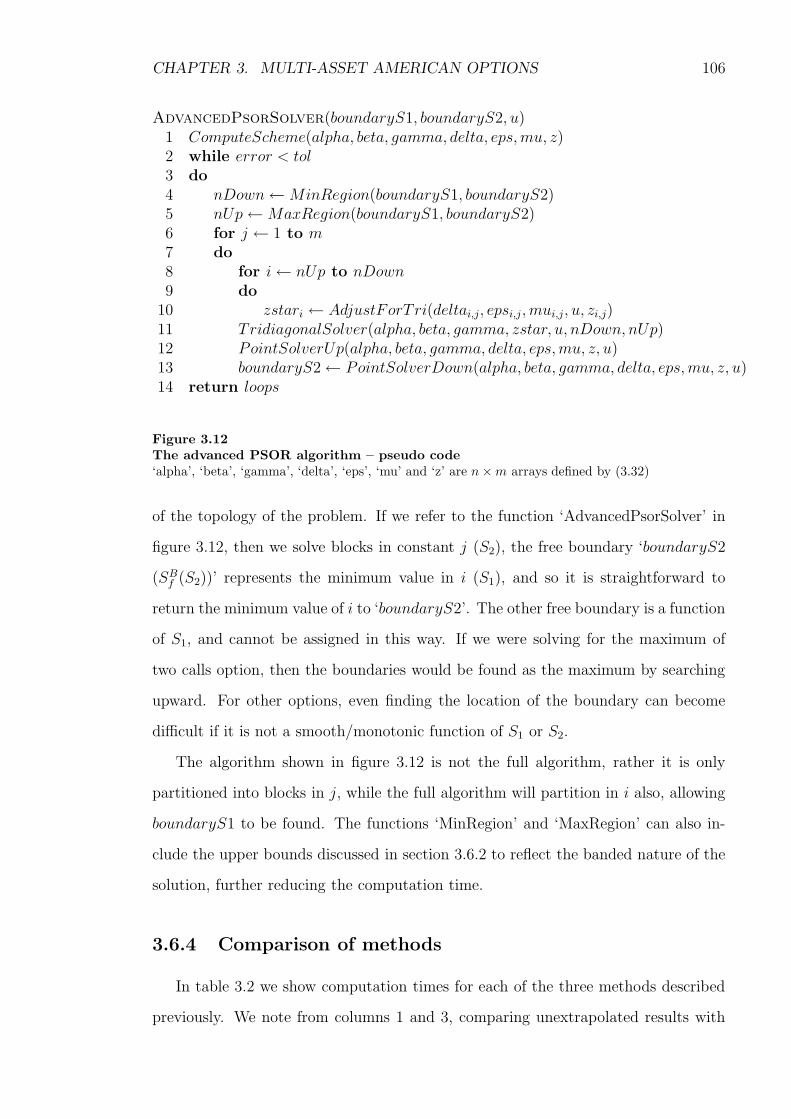
CHAPTER 3. MULTI-ASSET AMERICAN OPTIONS 106
AdvancedPsorSolver(boundaryS1, boundaryS2, u)1 ComputeScheme(alpha, beta, gamma, delta, eps,mu, z)2 while error < tol3 do4 nDown←MinRegion(boundaryS1, boundaryS2)5 nUp←MaxRegion(boundaryS1, boundaryS2)6 for j ← 1 to m7 do8 for i← nUp to nDown9 do
10 zstari ← AdjustForTri(deltai,j, epsi,j, mui,j, u, zi,j)11 TridiagonalSolver(alpha, beta, gamma, zstar, u, nDown, nUp)12 PointSolverUp(alpha, beta, gamma, delta, eps,mu, z, u)13 boundaryS2← PointSolverDown(alpha, beta, gamma, delta, eps,mu, z, u)14 return loops
Figure 3.12The advanced PSOR algorithm – pseudo code‘alpha’, ‘beta’, ‘gamma’, ‘delta’, ‘eps’, ‘mu’ and ‘z’ are n×m arrays defined by (3.32)
of the topology of the problem. If we refer to the function ‘AdvancedPsorSolver’ in
figure 3.12, then we solve blocks in constant j (S2), the free boundary ‘boundaryS2
(SBf (S2))’ represents the minimum value in i (S1), and so it is straightforward to
return the minimum value of i to ‘boundaryS2’. The other free boundary is a function
of S1, and cannot be assigned in this way. If we were solving for the maximum of
two calls option, then the boundaries would be found as the maximum by searching
upward. For other options, even finding the location of the boundary can become
difficult if it is not a smooth/monotonic function of S1 or S2.
The algorithm shown in figure 3.12 is not the full algorithm, rather it is only
partitioned into blocks in j, while the full algorithm will partition in i also, allowing
boundaryS1 to be found. The functions ‘MinRegion’ and ‘MaxRegion’ can also in-
clude the upper bounds discussed in section 3.6.2 to reflect the banded nature of the
solution, further reducing the computation time.
3.6.4 Comparison of methods
In table 3.2 we show computation times for each of the three methods described
previously. We note from columns 1 and 3, comparing unextrapolated results with
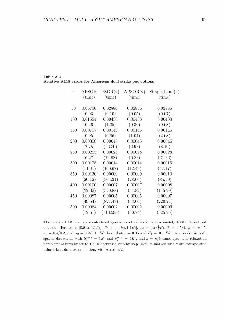
CHAPTER 3. MULTI-ASSET AMERICAN OPTIONS 107
Table 3.2Relative RMS errors for American dual strike put options
n APSOR PSOR(x) APSOR(x) Simple band(x)(time) (time) (time) (time)
50 0.06756 0.02886 0.02886 0.02886(0.03) (0.10) (0.05) (0.07)
100 0.01584 0.00438 0.00438 0.00438(0.26) (1.35) (0.30) (0.68)
150 0.00707 0.00145 0.00145 0.00145(0.95) (6.96) (1.04) (2.68)
200 0.00398 0.00045 0.00045 0.00046(2.75) (26.80) (2.97) (8.19)
250 0.00255 0.00028 0.00028 0.00028(6.27) (74.98) (6.82) (21.26)
300 0.00178 0.00014 0.00014 0.00015(11.81) (160.62) (12.49) (47.17)
350 0.00130 0.00009 0.00009 0.00010(20.12) (304.24) (28.60) (85.59)
400 0.00100 0.00007 0.00007 0.00008(32.02) (520.88) (34.82) (145.29)
450 0.00087 0.00005 0.00005 0.00007(49.54) (827.47) (53.60) (220.71)
500 0.00064 0.00002 0.00002 0.00006(72.51) (1132.98) (80.74) (325.25)
The relative RMS errors are calculated against exact values for approximately 4000 different put
options. Here S1 ∈ [0.9E1, 1.1E1], S2 ∈ [0.9E2, 1.1E2], E2 = E1/12E1, T = 0.5/1, ρ = 0/0.5,
σ1 = 0.4/0.2, and σ2 = 0.2/0.1. We have that r = 0.06 and E1 = 10. We use n nodes in both
spacial directions, with Smax1 = 5E1 and Smax
2 = 5E2, and k = n/5 timesteps. The relaxation
parameter ω initially set to 1.6, is optimised step by step. Results marked with x are extrapolated
using Richardson extrapolation, with n and n/2.

CHAPTER 3. MULTI-ASSET AMERICAN OPTIONS 108
extrapolated results, that although the convergence may not be exactly of order
O(∆S2,∆τ 2) (due to non-linear errors), the results are dramatically improved by
extrapolation, though not to the same extent as for the European prices (table 3.1).
The APSOR method, with boundary updating, is clearly far superior to both the base
method PSOR and also the simple banded solver. Notably, the APSOR method is
even faster at calculating American prices than the block solver was in solving for the
corresponding European price (table 3.1), mainly due to the fact we are only solving
in the important regions. Consequently the extra computational effort in locating the
free boundary (while simultaneously updating the solution) is offset by the enhanced
convergence of the scheme. We note here that for large n, the simple banded solver
does slightly worse than the other two methods. This may be because there may be
some regions over which we are not solving but should be. This is major drawback
in the method, namely that the position of the free boundary can only be guessed a
priori. If it is not guessed correctly, which is particularly difficult when volatility is
large, then errors may contaminate the entire solution.
3.7 Conclusions
The APSOR method proposed in this chapter is both fast and efficient as com-
pared to the standard PSOR method (around 15 times faster). For the continuously
exercised option the method is comparative to other methods in 2 and possibly 3
dimensions, although above this both the coding and calculation would become in-
creasingly difficult. However, the method is robust enough to handle a stochastic
interest rate as the second underlying, which will have applications, for instance, in
convertible bonds (chapter 6). As a result in low multi-dimensional problems the
method is fast and robust, with the added bonus that the optimal exercise barrier is
calculated at each time step for free.

Chapter 4
Time Dependent Barrier Options
The vanilla barrier option is a path-dependent option. Snyder (1969) describes
options of this type in detail, as well as the reasons why they may be traded. There are
four main types, ‘up-and-in’, ‘up-and-out’, ‘down-and-in’ and ‘down-and-out’. The
barrier is defined as the level in the asset space so that when the underlying asset
value crosses this point from above (down) or from below (up) the holder of the option
either receives (in) or has taken away (out) the rights to a European option of the
same maturity. While closed-form solutions have been found for simple vanilla barrier
options (Merton, 1990 shows that with a transform of variables the European ‘down-
and-out’ call option problem can be solved by using either separation of variables or
Fourier transform), the options can be extended to include early exercise or rebate,
resulting in a more complex problem which may require numerical solutions (Merton
also gives a solution for a ‘down-and-out’ call with rebate). The rebate takes the
form of a cash payment when the option is knocked out, or fails to knock in. When
early exercise is allowed, e.g. American-type barrier options, they can present an
interesting problem quite different from the standard American option if the location
of the optimal exercise boundary is close to the location of the barrier, since there may
be an interaction between the two. This results in different problems for numerical
solution, since there exist two locations for non-linearity errors. For instance, the
highly accurate scheme described in chapter 2 will not be as accurate here since the
grid may not be aligned with both the barrier and the optimal exercise boundary.
109
CHAPTER 4. TIME DEPENDENT BARRIER OPTIONS 110
The assumption of instant knock-out or knock-in may also be relaxed, allowing the
asset price to be above or below the barrier for a specified time before the option
is knocked in or out. Options where the barrier can be crossed for a predetermined
time are discussed next in section 4.1.
4.1 Occupation-Time Derivatives
Occupation-time derivatives are highly path-dependent options for which the time
spent above or below a barrier affects the payout of the option. Options of this form
include: Parisian and ParAsian (delayed barrier) options, switch and step options
(double barrier), and the α-quantile option (delayed look-back option).
The Parisian option is a barrier option for which the knock-in/out feature is only
realised when the stock has been above/below the barrier consecutively for a prede-
termined time. This class of option came to prominence for a number of reasons.
Straight barrier options are difficult to hedge (∆ = ∂V∂S
is discontinuous near the bar-
rier) and open to price manipulation. Also, when companies issue convertible bonds,
if they wish to embed an option to force conversion, this is normally undertaken with
reference to the stock price being above the call price for a certain amount of time,
i.e. a Parisian option.
Several papers have attempted to use occupation-time derivatives to model real
world occurrences. Gauthier (2000) uses the delayed nature of the Parisian option
in the analysis of real options. When valuing a real option in a project, there is
sometimes a delay between an investment decision and its implementation. The
delay is defined as the time the underlying asset spends above the threshold at which
it is optimal to invest. In another application, Francois and Morellec (2004) and
Moraux (2003) use down-and-out Parisian options to model Chapter 11 bankruptcy
and hence the default risk for bonds.
An obvious extension to the Parisian option is to count the time spent cumulatively
beyond the barrier. This has been dubbed the ParAsian option due to the Asian style
counting over the life of the option. Work performed by the author in collaboration

CHAPTER 4. TIME DEPENDENT BARRIER OPTIONS 111
with Yu (2004) argues that the cumulative nature of ParAsian options is better suited
to model Chapter 11, as the Parisian option barrier can be crossed and recrossed
numerous times without the option ever being knocked-out. Creditors may grow
weary of such a situation and decide to liquidate the bond. Model parameters and
the numerical scheme used to solve for such a bond are discussed in detail later in
chapter 5.
An even better model may be one that gives greater weight to the knockout time
when the asset value is further beneath the barrier. Creditors are likely to be far
more worried if the firm value drops to a very low level, even if it is just for a short
period of time; such an “Integral Time” model is proposed in this chapter.
The Parisian option can be simulated using the Monte-Carlo method, by simply
recording the length of time each path has spent beyond the barrier. There is, how-
ever, a possible bias linked to the discretisation of the problem, and the computation
time is slow. Due to this slow and cumbersome approach to pricing the option, the
options only caught the imagination of the finance community when Chesney et al.
(1997) priced them in a rigorous fashion. By using the theory of Brownian excursions,
they derive the price of a European Parisian option in terms of a Laplace transform,
that must then be inverted numerically. Others have since extended the approach to
the ParAsian option, which are found to be slightly easier to price than their Parisian
counterparts; Hugonnier (1999) presents an quasi-analytical pricing formula, as well
as numerous numerical results. However, Moraux (2002) notes that the results rep-
resented are not from the pricing formula itself, and, following the framework of
Chesney et al. (1997) and Hugonnier (1999) derives the proper closed-form solutions.
Strangely, though, no results are shown to back up these claims. Bernard et al. (2005)
develop a new inverse Laplace transform that improves on the method of Chesney et
al. (1997) to gain a fast solution to the Parisian problem. The most difficult part of
finding the solution via the method of Chesney et al. (1997) is to calculate the inverse
Laplace transform. They improve on this by approximating the function as the sum
of functions that have explicit inverse transforms. This allows the computation time
to be reduced significantly with minimal loss in accuracy.

CHAPTER 4. TIME DEPENDENT BARRIER OPTIONS 112
It is not immediately obvious as to how one would go about solving for the Parisian
option using lattice or finite-difference methods. Avellaneda and Wu (1999) make
three observations about the Parisian option in order to use a lattice method. Firstly,
when beyond the barrier, the option looks (and therefore hedges) like a knock-in
option, with maturity equal to time to knock-out, and a ‘rebate’ that equals the
value of the option at the barrier. Secondly, when the asset price has not crossed
the barrier, the option can be viewed as a knock-out option with the same maturity
and a rebate that equals the option value at the barrier. Thirdly, the option value at
the barrier is determined by imposing a smooth pasting condition, namely that the
derivative of the option value is continuous across the barrier; this can be justified
by no-arbitrage arguments. From these observations, they conclude that the problem
may be split into two coupled options, one which must be solved above the barrier,
and one to be solved below the barrier. They use a trinomial tree approach but
conclude that in the continuous time limit, the problem is in fact two coupled PDEs,
and a Crank-Nicolson scheme could also be applied without loss of generality. They
also express the approach in the limit of continuous time as an integral, suggesting
that quadrature methods may be applied, possibly more successfully than lattice
or finite-difference methods. However, the smooth pasting condition at the barrier
becomes very complicated when expressed in integral form. Costabile (2002) uses
the framework of Cox et al. (1979) to construct a binomial tree method which is
fast, but as with all lattice methods, the method is not flexible enough to include
cumulative time spent under the barrier or other modifications to time under the
barrier. Kwok and Lau (2001) use a forward shooting algorithm, pioneered by Hull
and White (1993) and others. This is an extension to the usual binomial or trinomial
trees, where an extra auxiliary state vector is used at each node to capture the path
dependency of the option. This has the advantage that it can handle situations where
the governing PDE is not simple and the asset value is not monitored continuously.
Haber et al. (1999) derive the PDE for the occupation-time derivative, and propose
an explicit finite-difference scheme with which to solve the problem. The finite-
difference method is flexible and is easily modified to include features such as early

CHAPTER 4. TIME DEPENDENT BARRIER OPTIONS 113
exercise, rebates and cumulative time spent under the barrier. Zhu and Stokes (1999)
develop a finite-element approach to the problem of Parisian options using the PDE
approach. This has the advantage that the elements can be refined in areas where
it is needed to improve the accuracy of the solution. Whether or not the method
is easily extended to include early exercise is unclear, though Crank (1984) states
that the Projected SOR algorithm can be used just as easily on finite-element as
finite-difference schemes.
Studying practitioners’ procedure, Anderluh and van der Weide (2004) seek an
implied barrier. Most practitioners hedge and price Parisian options as straight bar-
rier options with barriers slightly above or below that stated in the contract. They
use Brownian excursion theory (Revuz and Yor, 1999) to model what this difference
should be. The errors with this scheme are highly dependent on the barrier time,
which is reasonable since Parisian options tend to the straight/fixed barrier as the
barrier time is reduced. They do find a close match to the ∆ hedge though, which is
probably explained by the observations made by Avellaneda et al. (1999) (that the
option out of the barrier is like a knock-out option with rebate).
Chesney and Gauthier (2006) note that the vast majority of previous literature
focuses on European options, with only a brief mention of American options in Haber
et al. (1999). They study the similarities between American barrier options, which
have closed form solutions in the perpetual case (Russian options) and the American
Parisians. They show that American Parisians also have a closed-form solution in the
perpetual case. Using a probabilistic approach they reformulate the non-perpetual
case into a function of the exercise boundary. A corresponding equation for the
exercise boundary is also therefore required to solve for the option value.
To summarise, there are four possible methods with which to solve time-dependent
derivatives: simulation, lattice, Laplace transform and PDE. The major disadvantage
of the Laplace method is its inflexibility, while the simulation and lattice methods
are very slow. For its flexibility, we choose to extend the finite-difference method
as proposed by Haber et al. (1999). Using a Crank-Nicolson discretisation with
relatively large time steps, the solution time can be significantly reduced so as to

CHAPTER 4. TIME DEPENDENT BARRIER OPTIONS 114
allay the fears of Bernard et al. (2005) and others.
4.2 Parisian Options
Let us define a variable to represent the time spent above (below) the barrier, t
(the barrier-clock). Now let H be the barrier level for which the asset value must
spend time above or below. When the asset value is beyond the barrier, and if the
barrier-clock moves at the same rate as real time t, then dt = dt. When the asset
value has not crossed the barrier, then the barrier-clock does not advance in time and
dt = 0. When the asset price hits the barrier after it has gone beyond the barrier,
the barrier-clock is reset to zero again. For an up option, we can write
dt =
0 if S(t) < H
dt if S(t) > H, (4.1)
where the counter resets to zero when S(t) = H . The knock-in/out effects will be
triggered when the barrier-clock reaches some pre-specified level, say t = T , where T
is sometimes referred to as the length of the window.
The option value V , is now a function of three state variables, S, t and t, so we
have V = V (S, t, t ). Let us assume a BSM framework with constant drift, volatility
and interest rate. Then S follows a log-normal geometric Brownian motion and the
small change in asset price is given by
dS
S= µdt+ σdX (4.2)
From Ito calculus, it follows that the small change in option price is given by
dV = σS∂V
∂SdX +
(
µS∂V
∂S+
1
2σ2S2∂
2V
∂S2+∂V
∂t
)
dt+∂V
∂tdt,

CHAPTER 4. TIME DEPENDENT BARRIER OPTIONS 115
given that dt = O(dt). From (4.1), the small change in option price becomes
dV =
σS∂V
∂SdX +
(
µS∂V
∂S+
1
2σ2S2∂
2V
∂S2+∂V
∂t
)
dt if S(t) < H
σS∂V
∂SdX +
(
µS∂V
∂S+
1
2σ2S2∂
2V
∂S2+∂V
∂t+∂V
∂t
)
dt if S(t) > H,(4.3)
here dt = dt. On the barrier, the value of barrier-clock is reset to zero, so to maintain
path continuity the value of the option for all t must be equal to the value at of the
option when t = 0. Hence we need only solve V (H, t, t ) for t = 0. Consequently, for
a small change in V when the asset price is at the barrier we also have
dV = σS∂V
∂SdX +
(
µS∂V
∂S+
1
2σ2S2∂
2V
∂S2+∂V
∂t
)
dt (4.4)
By constructing a hedging portfolio in the usual way we arrive at the following
PDEs, which are valid over different regions of S and t
∂V
∂t+
1
2σ2S2∂
2V
∂S2+ (r − d)S∂V
∂S− rV = 0, S < H, (4.5)
∂V
∂t+∂V
∂t+
1
2σ2S2∂
2V
∂S2+ (r − d)S.∂V
∂S− rV = 0, S > H. (4.6)
When the asset value is below the barrier, S < H , then we must solve (4.5) with
t = 0, since the barrier-clock is always zero below the barrier. If the asset value is
at the barrier, the clock is reset to zero. When the asset value is above the barrier,
S > H , we solve (4.6) for t < T , where the additional ∂V/∂t term indicates that
the clock is ticking.
4.2.1 Parisian Options – Boundary Conditions
For a Parisian option, the clock is reset to zero when S = H , then we must
maintain continuity across paths, which gives rise to
V (S = H, t, t ) = V (S = H, t, 0). (4.7)

CHAPTER 4. TIME DEPENDENT BARRIER OPTIONS 116
In order to satisfy the BSM equation we must also maintain a continuous hedge across
the barrier. Since all paths cross at t = 0, we require
limS↑H
∂V
∂S(S, t, 0) = lim
S↓H
∂V
∂S(S, t, 0), (4.8)
where ∆ = ∂V/∂S is the usual BSM hedge.
There are many variants of the Parisian option: up/down, in/out on any number
of possible payoffs. We specify here that the payoff of the option, when it is knocked-
in/out at t = T , is G(S, t ), and the terminal condition, if the option is not knocked-
in/out, is F (S, t ). Then we have
V (S, T, t ) = F (S, t ) for 0 ≤ t < T ,
V (S, t, T ) = G(S, t ).
For example, on a Parisian up-and-out call, we have F (S, t ) = max[0, S − E] and
G(S, t ) = 0.
At extremes in the asset value we have to take into account the difference between
the time-to-knockout (TTK) and the time-to-maturity (TTM). For example, let us
examine the up-and-out call option. If the TTK is less than or equal to the TTM,
then as S →∞ the option is almost certain to be above the barrier until it is knocked
out, so
V (S →∞, t, t )→ 0 if (T − t ) ≤ (T − t).
However, if TTK is greater than TTM, then there is no chance that the option can
be knocked out, and the option value behaves like a standard call option,
V (S →∞, t, t )→ Se−d(T−t) − Ee−r(T−t) if (T − t ) > (T − t).
Hence, there is an apparent discontinuity in the option value above the barrier if t is
held constant, and we move in t across the point t = t, or vice versa. However, the
discontinuity does not really exist as it is not possible for the option value above the

CHAPTER 4. TIME DEPENDENT BARRIER OPTIONS 117
barrier to move in real time without the barrier-clock advancing at the same rate.
4.2.2 Numerical Method
The scheme adopted here is based on the Crank-Nicolson method, considered in
chapter 1. The Crank-Nicolson scheme is second-order accurate and unconditionally
stable (at least in the European case). These two factors become especially important
when pricing occupational time derivatives. With two time variables to consider, the
storage requirements are restricted by the number of timesteps used. At each point
in real time, the value of the option for all values of barrier time must to be stored,
in addition to all asset values. Consequently, if the number of timesteps is doubled,
then so is the storage requirement. Hence, the number of nodes over which we must
solve at each timestep will also double, resulting in a (minimum) fourfold increase
in computation time. Consequently, the ability to gain accurate results with a small
number of timesteps will greatly increase the efficiency of the solution.
Since we solve backwards in time, we define two modified variables τ and τ , such
that
0 < τ = T − t < T, 0 < τ = T − t < T .
Using this change of variables in (4.5) and (4.6) we have the following PDEs,
Vτ + Vτ =1
2σ2S2VSS + (r − d)SVS − rV (4.9)
Vτ =1
2σ2S2VSS + (r − d)SVS − rV. (4.10)
The PDE (4.10) can be discretised in the standard fashion. However (4.9) is a little
unusual as it has two time derivatives. Discretising according to the Crank-Nicolson
method, the left hand side of (4.9) becomes
Vτ + Vτ ≃1
2
{
1
∆τ(vk+1,l+1
i − vk,l+1i ) +
1
∆τ(vk+1,l
i − vk,li )
}
+1
2
{
1
∆τ(vk+1,l+1
i − vk+1,li ) +
1
∆τ(vk,l+1
i − vk,li )
}
, (4.11)

CHAPTER 4. TIME DEPENDENT BARRIER OPTIONS 118
where V (i ·∆S, k ·∆τ, l ·∆τ ) = vk,li . The PDE (4.9) is derived from (4.1) with dt = dt,
so we may set ∆τ = ∆τ , and then (4.11) becomes
Vτ + Vτ =1
∆τ(vk+1,l+1
i − vk,li ). (4.12)
The discretisation of (4.11) uses the four time points at nodes (k, l), (k, l+1), (k+1, l)
and (k + 1, l + 1) and for second-order accuracy, the right hand side should be the
average over all four nodes. However, our choice of ∆τ = ∆τ leads to fortuitous
cancellations taking place, resulting in a discretisation over just the two nodes (k, l)
and (k+ 1, l+ 1), and therefore we can maintain second-order accuracy on the right-
hand-side averaging over just those two nodes. By using just two nodes storage
requirements are reduced; we need only store values at one timestep. It is not required
that ∆τ = ∆τ in order to solve the PDE. In fact, if ∆τ 6= ∆τ then the cancellations
do not take place and we will need to use all four nodes on the right hand side.
Also there will be stability issues (which are discussed later in section 4.4), increased
storage and iteration (Parisian option only) in this case.
4.2.3 Two Numerical Schemes
We present two possible schemes using either two or four nodes. Scheme 1 has
the restriction ∆τ = ∆τ whereas we are free to choose ∆τ in Scheme 2. The latter
is more flexible, but it comes at a price: the scheme can oscillate violently.
Scheme 1
For an ‘up’ option we can form the following set of equations,
αivk+1,l+1i−1 + (
1
∆τ+ βi)v
k+1,l+1i + γiv
k+1,l+1i+1 = Zk,l+1
i if i < hi,
αivk+1,l+1i−1 + (
1
∆τ+ βi)v
k+1,l+1i + γiv
k+1,l+1i+1 = Zk,l
i if i ≥ hi. (4.13)

CHAPTER 4. TIME DEPENDENT BARRIER OPTIONS 119
where the position of the barrier is hi = NINT(
H∆S
)
and
Zk,li = −αiv
k,li−1 + (
1
∆τ− βi)v
k,li − γiv
k,li+1.
To avoid non-linearity errors in the scheme, it is best to set ∆S such that
ei ·∆S = E,
hi ·∆S = H,
where ei and hi are integers, and also ∆τ so that
tk ·∆τ = T,
tl ·∆τ = T ,
where tk and tl are integers.
Scheme 2
If we discretise with ∆τ 6= ∆τ then,
αivk+1,l+1i−1 + (
1
∆τ+ βi)v
k+1,l+1i + γiv
k+1,l+1i+1 = Zk,l+1
i
if i < hi,
1
2αiv
k+1,l+1i−1 +
1
2
(
1
∆τ+
1
∆τ+ βi
)
vk+1,l+1i +
1
2γiv
k+1,l+1i+1 = W k,l
i
if i ≥ hi. (4.14)
where
W k,li = −1
2αiv
k,li−1 +
1
2
(
1
∆τ+
1
∆τ− βi
)
vk,li −
1
2γiv
k,li+1
−1
2αiv
k,l+1i−1 +
1
2
(
1
∆τ− 1
∆τ− βi
)
vk,l+1i − 1
2γiv
k,l+1i+1
−1
2αiv
k+1,li−1 −
1
2
(
1
∆τ− 1
∆τ+ βi
)
vk+1,li − 1
2γiv
k+1,li+1 . (4.15)
(4.16)

CHAPTER 4. TIME DEPENDENT BARRIER OPTIONS 120
This scheme is also valid when ∆τ = ∆τ but only has the same accuracy as Scheme
1.
4.2.4 Implementing the Schemes on a Parisian Option
When solving for the Parisian option to obtain a consistent solution we must
ensure that the continuity of paths condition (4.7) is satisfied. Let us consider Scheme
1 first, for an up-and-out option. To start, we must find the value of the option at
the barrier. This is found by solving (4.13) with l = tl for all i. Then we set
vk+1,lhi
= vk+1,tlhi
for 0 < l < tl.
For the remaining values of v with 0 < l < tl, we now solve the second part of (4.13)
(with Zk,li ) over the region hi < i < n with the usual boundary condition for v at
i = n and the condition above for v at i = hi, again to reduce the storage requirement
we solve from l = tl − 1 to l = 1.
When using Scheme 2, we see that this is not actually explicit, and we need to
iterate in order to find the solution; this is as a result of condition (4.7). In order to
solve for v at l = tl, we must determine the value at l = tl − 1, but this value cannot
be calculated without the boundary condition given by (4.7). Consequently, in order
to estimate the value at the barrier we solve for v with
αi
(
vk+1,tli−1
)q+1
+ (1
∆τ+ βi)
(
vk+1,tli
)q+1
+ γi
(
vk+1,tli+1
)q+1
= Zk,tli if i < hi,
1
2αi
(
vk+1,tli−1
)q+1
+1
2
(
1
∆τ+
1
∆τ+ βi
)
(
vk+1,tli
)q+1
+1
2γi
(
vk+1,tli+1
)q+1
=(
W k,tl−1i
)q
if i ≥ hi,
at the (q + 1)th iteration. The right-hand side(
W k,tl−1i
)q
uses the qth iteration

CHAPTER 4. TIME DEPENDENT BARRIER OPTIONS 121
(
vk+1,tl)q
as a guess for the value at the current time step. Next we solve
1
2αi
(
vk+1,l+1i−1
)q+1
+1
2
(
1
∆τ+
1
∆τ+ βi
)
(
vk+1,l+1i
)q+1
+1
2γi
(
vk+1,l+1i+1
)q+1
=(
W k,li
)q+1
,
over hi < i < n moving from l = 1 to l = tl − 1, with
(
vk+1,lhi
)q+1
=(
vk+1,tlhi
)q+1
.
We can use the (q+1)th estimate for W if we use the most up to date value at l− 1.
The scheme does converge, but significantly slower if the qth estimate is used.
4.3 ParAsian Options
An obvious extension to the Parisian option is the ParAsian option. For a Parisian,
if the asset price were to fluctuate above and below the barrier, it is possible that the
option would not be knocked-in/out even though it may have spent a considerable
time over the barrier. Hence we define the ParAsian option to be the cumulative time
spent over the barrier. It turns out that these options can be priced more easily than
their Parisian counterparts, because of not having to reset the clock at the barrier.
The formulation of this class of option is essentially the same as for the Parisians,
except that we must now solve over all values of t even when the asset price is not
beyond the barrier, since the clock retains its value even when it is not ticking. The
change in barrier-clock is now defined as
dt =
0 if S(t) < H
dt if S(t) ≥ H, (4.17)
where the ParAsian option here is of the ‘up’ variety. The boundary condition (4.7)
is not required as the clock is not reset.
Using the BSM framework as above, we arrive at the same two PDEs as before,
CHAPTER 4. TIME DEPENDENT BARRIER OPTIONS 122
(4.5) and (4.6), except they are valid over different regions. For an up (down) option,
we must solve (4.5) for t < T when the asset price is below (above) the barrier, and
(4.5) for t < T when the asset value is at or above (below) the barrier.
4.3.1 ParAsian Options – Boundary Conditions
There is no condition on the value of the ParAsian option at the barrier since the
clock is not reset. Nevertheless, we must still maintain the continuity of both V and
its first derivative ∂V∂S
across the barrier, resulting in the following equations
limS↑H
V (S, t, t ) = limS↓H
V (S, t, t ), (4.18)
limS↑H
∂V
∂S(S, t, t ) = lim
S↓H
∂V
∂S(S, t, t ). (4.19)
Any solution of the BSM PDE will be at least C1 continuous so will satisfy both
(4.18) and (4.19). However, this condition becomes important, later in chapter 7,
when we study the delayed-exercise option, and these conditions are used to derive
the position of the barrier. Otherwise, boundary conditions for ParAsian options will
be interchangeable with those for Parisian options.
4.3.2 Implementing the schemes on a ParAsian Option
Implementing schemes on a ParAsian option is significantly easier than in the case
of a Parisian option, and so we deal with the former case first. First, let us consider
scheme 1. At each timestep simply solve (4.13) for 0 < l ≤ tl in the appropriate
regions in S depending on whether the option is ‘down’ or ‘up’. We may also have to
solve for the corresponding European (or American) option which the holder receives
if the option is an ‘in’ option. Hence, for the ‘in’ option
vk,0i = VE(S, τ),

CHAPTER 4. TIME DEPENDENT BARRIER OPTIONS 123
otherwise if the option is ‘out’ then
vk,0i = 0.
Since vk+1,l+1 depends on vk,l+1 and vk,l, then the scheme can be solved backwards
from l = tl to l = 1 so that v need only be stored at one time level, namely k.
For Scheme 2, (4.14) is implemented on the appropriate regions. Now vk+1,l+1
depends on vk,l+1, vk+1,l, and vk,l, so the scheme must be stored at two time levels k
and k + 1 and solved forwards from l = 1 to l = tl so that the updated vk+1,l can be
used to solve for vk+1,l+1.
4.4 Results
We compare our results to those of Haber et al. (1999) (obtained using an explicit
scheme) for the up-and-out call. Scheme 1 with ∆τ = ∆τ is compared to Scheme 2
with varying ∆τ . It is well known that a central-difference scheme such as Crank-
Nicolson, while being efficient and accurate for smooth solutions, has difficulty dealing
with discontinuous solutions. As described earlier, such a discontinuity propagates
along the line τ = τ (beyond the barrier), where the option value is either almost
definitely knocked out (τ > τ ), or will definitely reach maturity and gain a payoff
(τ < τ ). It would be unreasonable to assume that there is not a possibility that
the solution may oscillate in this region in the common phenomenon experienced by
central-differencing schemes. In figure 4.1, the solution in such a region is investigated.
The four diagrams represent four possible cases. The variation of a Parisian option
value is shown with τ , for an up-and-out call with barrier H = 12; the time-to-
maturity τ = 0.01. The five plots indicate the value of the option at S = 12, though
to 12.225 with intervals of 0.025. This region is shown as it is the most sensitive
and has greatest influence on the option value below the barrier (the value below
the barrier is unconditionally stable since the option cannot be knocked out in this
region). The horizontal line in all four figures is the value at S = 12; at the barrier the

CHAPTER 4. TIME DEPENDENT BARRIER OPTIONS 124
0
0.5
1
1.5
2
2.5
0.10.0750.050.0250
Opti
onV
alueV
(S,τ,τ
)
τ
(a) (Scheme 1) ∆τ = ∆τ
0
0.5
1
1.5
2
2.5
3
0.10.0750.050.0250
Opti
onV
alueV
(S,τ,τ
)
τ
(b) (Scheme 2) ∆τ > ∆τ
0
0.5
1
1.5
2
2.5
0.10.0750.050.0250
Opti
onV
alueV
(S,τ,τ
)
τ
(c) (Scheme 2) ∆τ = ∆τ
-0.5
0
0.5
1
1.5
2
2.5
0.10.0750.050.0250
Opti
onV
alueV
(S,τ,τ
)
τ
(d) (Scheme 2) ∆τ < ∆τ
Figure 4.1Parisian up-and-out option vs. time-to-knockout close to maturityThe value of a Parisian up-and-out option against time-to-knockout for S = 12 through to 12.225
with intervals of 0.025. Here E = 10, H = 12, σ = 0.2, r = 0.05, and τ = 0.1
value is constant across τ from condition (4.7). As τ ≫ τ then the value approaches
the vanilla call option price; the maximum occupation time is T = 0.1.
The value calculated by Scheme 1 is shown in figure 4.1(a). The value appears
smooth and the sharp wave form at τ = τ = 0.01 is maintained. For Scheme 2, how-
ever, things deteriorate. When ∆τ > ∆τ (figure 4.1(b)) the solution has oscillations
that are both large and move past the point at which τ = τ . When ∆τ < ∆τ the so-
lution seems satisfactory when τ > τ (there is some smoothing of the discontinuity),
but there are large and violent oscillations in the solution when τ < τ resulting in er-
roneous negative option values. Even when ∆τ = ∆τ there are still small oscillations
either side of τ = τ .
Nonetheless, as τ increases, the oscillations become damped, and the solution at

CHAPTER 4. TIME DEPENDENT BARRIER OPTIONS 125
0
0.02
0.04
0.06
0.08
0.1
0.12
0.14
0.16
0.18
0.2
0.10.0750.050.0250
Opti
onV
alueV
(S,τ,τ
)
τ
(a) (1) ∆τ = ∆τ
0
0.02
0.04
0.06
0.08
0.1
0.12
0.14
0.16
0.18
0.2
0.10.0750.050.0250O
pti
onV
alueV
(S,τ,τ
)
τ
(b) (2) ∆τ > ∆τ
0
0.02
0.04
0.06
0.08
0.1
0.12
0.14
0.16
0.18
0.2
0.10.0750.050.0250
Opti
onV
alueV
(S,τ,τ
)
τ
(c) (2) ∆τ = ∆τ
0
0.02
0.04
0.06
0.08
0.1
0.12
0.14
0.16
0.18
0.2
0.10.0750.050.0250
Opti
onV
alueV
(S,τ,τ
)
τ
(d) (2) ∆τ < ∆τ
Figure 4.2Parisian up-and-out option value vs. time-to-knockout.The value of a Parisian up-and-out option against time-to-knockout for S = 12 through to 12.225
with intervals of 0.025. Here E = 10, H = 12, σ = 0.2, r = 0.05, and τ = 1

CHAPTER 4. TIME DEPENDENT BARRIER OPTIONS 126
τ = T appears to be smooth. Figure 4.2 shows the same option values evaluated
with the same schemes at τ = 1 (so that τ ≫ τ ). The solutions for ∆τ > ∆τ still
appear to be slightly oscillatory. It may be possible to damp down these oscillations
by reducing ∆τ , however, when ∆τ ≤ ∆τ the oscillations become damped and the
solutions appear accurate and reliable.
4.4.1 Parisian Options
The following results in figures 4.3–4.5 are comparable to those of Haber et al.
(1999). In figure 4.3 the value of a Parisian up-and-out call option is shown. The
parameters are: σ = 0.2, r = 0.05, τ = 0.1, T = 1 and H = 12. When S is small and
far from the barrier, the option behaves as a vanilla call option. As the asset price
approaches the barrier, the value of the option is dragged down as the probability
that it will be knocked out at some time during the lifetime of the option is increased.
For S greater than H , the option value behaves as a knockout option with a rebate of
V (S = H, τ, T ). The value of the delta is continuous across the barrier at τ = T , but
has a large discontinuity at the barrier for all other values of τ ; the delta is strictly
negative above the barrier.
In figure 4.3(a) the value of the option for very small τ is shown. Above the
barrier the option is practically worthless, since the option is almost knocked out. If
the asset value is close to the barrier, there may be a slight chance that the asset
value will hit the barrier before it is knocked out, and there will be a large positive
jump in the value of the option. This results in a large negative value of the delta;
this situation is not as prominent as the situation for a barrier option, where small
price movements can have a large effect on the hedging strategy (whenever the asset
price is close to the barrier). Here, only when the asset has followed a particular path
will the situation arise, and hence, the probability of a practitioner having to hedge
in such a way is unlikely. It is, however, a problem that can be overcome by taking
the cumulative time spent over the barrier rather than the consecutive time.
The convergence of the Crank-Nicolson numerical scheme is shown in table 4.1.
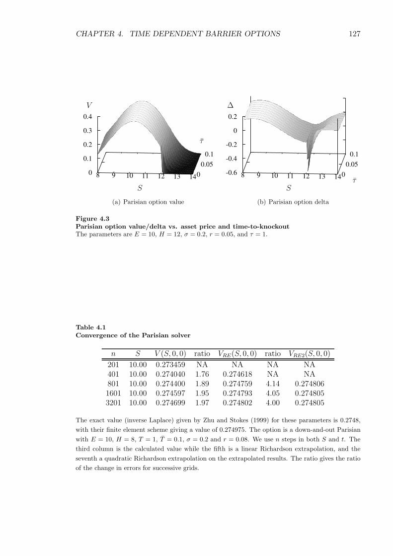
CHAPTER 4. TIME DEPENDENT BARRIER OPTIONS 127
8 9 10 11 12 13 14
0.1
0.05
0
0.4
0.3
0.2
0.1
0
V
S
τ
(a) Parisian option value
8 9 10 11 12 13 14
0.1
0.05
0
0.2
0
-0.2
-0.4
-0.6
∆
Sτ
(b) Parisian option delta
Figure 4.3Parisian option value/delta vs. asset price and time-to-knockoutThe parameters are E = 10, H = 12, σ = 0.2, r = 0.05, and τ = 1.
Table 4.1Convergence of the Parisian solver
n S V (S, 0, 0) ratio VRE(S, 0, 0) ratio VRE2(S, 0, 0)
201 10.00 0.273459 NA NA NA NA401 10.00 0.274040 1.76 0.274618 NA NA801 10.00 0.274400 1.89 0.274759 4.14 0.2748061601 10.00 0.274597 1.95 0.274793 4.05 0.2748053201 10.00 0.274699 1.97 0.274802 4.00 0.274805
The exact value (inverse Laplace) given by Zhu and Stokes (1999) for these parameters is 0.2748,
with their finite element scheme giving a value of 0.274975. The option is a down-and-out Parisian
with E = 10, H = 8, T = 1, T = 0.1, σ = 0.2 and r = 0.08. We use n steps in both S and t. The
third column is the calculated value while the fifth is a linear Richardson extrapolation, and the
seventh a quadratic Richardson extrapolation on the extrapolated results. The ratio gives the ratio
of the change in errors for successive grids.

CHAPTER 4. TIME DEPENDENT BARRIER OPTIONS 128
Table 4.2Comparison of results
Crank-Nicolson ExplicitS t = 0 t = 0.05 t = 0.095 t = 0 t = 0.05 t = 0.095
11.05 0.3318 0.3318 0.3318 0.2783 0.2783 0.278311.24 0.3106 0.3106 0.3106 0.2566 0.2566 0.256611.43 0.2851 0.2851 0.2851 0.2314 0.2314 0.231411.62 0.2557 0.2557 0.2557 0.2030 0.2030 0.203011.81 0.2228 0.2228 0.2228 0.1719 0.1719 0.171912.01 0.1870 0.1859 0.1781 0.1387 0.1242 0.062212.21 0.1494 0.1315 0.0397 0.1062 0.0814 0.000012.42 0.1132 0.0839 0.0027 0.0771 0.0478 0.000012.63 0.0811 0.0480 0.0000 0.0529 0.0249 0.000012.84 0.0549 0.0244 0.0000 0.0342 0.0113 0.000013.06 0.0351 0.0110 0.0000 0.0208 0.0044 0.000013.28 0.0211 0.0044 0.0000 0.0118 0.0014 0.000013.50 0.0120 0.0016 0.0000 0.0063 0.0004 0.000013.73 0.0064 0.0005 0.0000 0.0031 0.0001 0.000013.96 0.0032 0.0001 0.0000 0.0014 0.0000 0.0000
Comparison of results between the Crank-Nicolson scheme used here, and the explicit scheme used
in Haber et al. (1999). The option being valued is an up-and-out Parisian with E = 10, H = 12,
T = 1, T = 0.1, σ = 0.2 and r = 0.05. The Crank-Nicolson scheme uses extrapolated results from
801, 1601 and 3201 node (both S and t) calculations.
We see that second order convergence from the scheme is lost due to the errors
described earlier, with the ratio for the unextrapolated results around 2. However,
linear Richardson extrapolation leads to results that show second order convergence
(ratio around 4), which can then be extrapolated a further time to yield highly
accurate results.
In table 4.2, we compare our results to those of Haber et al. (1999). Our results
have been interpolated from a uniform grid in S, to match those from the transformed
grid of Haber et al. (1999). Since Haber et al. (1999) do not present any convergence
analysis, we can only conclude that the explicit scheme is not even remotely accurate,
with large errors contaminating the entire solution. Anyone wishing to solve for a
Parisian option with an explicit finite difference scheme must therefore be wary of
potentially huge errors.

CHAPTER 4. TIME DEPENDENT BARRIER OPTIONS 129
8 9 10 11 12 13 14
0.1
0.05
0
0.4
0.3
0.2
0.1
0
V
S
τ
(a) ParAsian Option Value
8 9 10 11 12 13 14
0.1
0.05
0
0.2
0
-0.2
0.1
-0.1
∆
S
τ
(b) ParAsian Option Delta
Figure 4.4ParAsian option value/delta vs. asset price and time-to-knockoutThe parameters are E = 10, H = 12, σ = 0.2, r = 0.05, and τ = 1.
4.4.2 ParAsian Options
The ParAsian option exhibits a smoother solution, due to the continuity of the
first derivative with respect to asset price S over the solution space. The ParAsian
option is more likely to be knocked out than its Parisian counterpart, which causes
the price of the option to drop accordingly. Since the ParAsian option is solved over
the entire state space, we have a solution at every point even below the barrier and
it can be seen that
limτ→0
V (S, τ, τ ) = VB(S, τ),
where VB(S, τ) is the value of the corresponding straight barrier option. Again, when
τ → 0 and S is close to but not beyond the barrier H , there will be sharp movements
in the delta. Figure 4.4 shows the option price and its delta, which is now continuous
and of much smaller magnitude than its Parisian counterpart.
Figure 4.5 compares the magnitude of the Parisian price and the ParAsian price.
The lower price of the ParAsian would be attractive to purchasers of the option
(one of the main reasons for buying the barrier option is because it is cheaper than
the corresponding vanilla) and it also appears that it will be easier to hedge than
the corresponding Parisian. The large discontinuity in the hedging strategy across
the barrier of the Parisian exposes the writer of the option to a large amount of

CHAPTER 4. TIME DEPENDENT BARRIER OPTIONS 130
0
0.05
0.1
0.15
0.2
0.25
0.3
0.35
0.4
8 9 10 11 12 13 14
V
S(a) Option Value
-1
-0.8
-0.6
-0.4
-0.2
0
0.2
8 9 10 11 12 13 14
∆
S(b) Option Delta
Figure 4.5Parisian/ParAsian option value/delta vs. asset price.The ParAsian option (solid line) and the Parisian option (dashed line), are shown for differing
time-to-knockout. Again the parameters are E = 10, H = 12, σ = 0.2, r = 0.05, and τ = 1
risk, indicated by the delta. The value of the gamma gives some indication into the
risk exposure of the delta hedge and is discontinuous across the barrier even for the
ParAsian. In the next section, the IT option has a solution which is continuous in
both its delta and gamma, and therefore has less risk involved in hedging.
4.5 A New Option – The Integral Time Model
Even though the Parisian options were created to ease hedging around the barrier,
some problems still exist, which led Linetsky (1999) to propose the step option, in
which the payoff at the end is proportional to the time spent under the barrier. By
removing large jumps in the payoff the hedging strategy of the option is smoother. For
a similar reason, we propose the integral time ParAsian option which has a smoother
transition across the barrier than the ParAsian or Parisian. An option of this form
has been investigated by Xiao (2007) with regard to foreign exchange options. In
the paper by Haber et al. (1999) it is suggested that it would be simple to modify
the behaviour of the barrier-clock so that, for instance, more weight could be given
according to the size of deviations above (below) the barrier. Let us examine such a
model with a cumulative clock, for an up option with barrier H ; let the integral I be

CHAPTER 4. TIME DEPENDENT BARRIER OPTIONS 131
defined as
I =
∫ t
0
dI(t),
where
dI =
0 if S(t) < H
χ(S(t)−H)dt if S(t) ≥ H. (4.20)
Such a situation is shown in figure 4.6. The shaded area indicates the area between
the barrier H (here H = 1.4) and the asset price. The parameter χ, used to scale
the deviations over the barrier, is dimensionless since I has units [S× t]. If S follows
the usual geometric Brownian motion in (4.2) then the small change in option price
becomes
dV = σS∂V
∂SdX +
(
µS∂V
∂S+
1
2σ2S2∂
2V
∂S2+∂V
∂t
)
dt+∂V
∂IdI,
and using the appropriate form for dI we obtain the following
dV =
σS∂V
∂SdX +
(
µS∂V
∂S+
1
2σ2S2∂
2V
∂S2+∂V
∂t
)
dt
if S(t) < H
σS∂V
∂SdX +
(
µS∂V
∂S+
1
2σ2S2∂
2V
∂S2+∂V
∂t+ χ(S −H)
∂V
∂I
)
dt
if S(t) ≥ H .
(4.21)
Then, setting up the BSM hedging portfolio as usual we arrive at the following two
PDEs
∂V
∂t+
1
2σ2S2∂
2V
∂S2+ (r − d)S∂V
∂S− rV = 0 if S < H, (4.22)
χ(S −H)∂V
∂I+∂V
∂t+
1
2σ2S2∂
2V
∂S2+ (r − d)S∂V
∂S− rV = 0 if S ≥ H. (4.23)
We call this new class of options Integral Time (IT) options. The option de-
scribed here is a ParAsian IT option; however, there are many possible variations of
the IT option. The option can be up/down, in/out, Parisian/ParAsian, or have a
second barrier (step or switch type option). The option may also depend on the time

CHAPTER 4. TIME DEPENDENT BARRIER OPTIONS 132
0.9
1
1.1
1.2
1.3
1.4
1.5
1.6
1.7
0 0.05 0.1 0.15 0.2 0.25 0.3 0.35 0.4 0.45 0.5
Ass
etP
riceS
Time t
Figure 4.6A Monte-Carlo simulation of how the area over the barrier is formed.
spent over the barrier as well as the area over the barrier. We concentrate here on
the ParAsian IT option and present some interesting findings about the associated
Greeks.
4.5.1 Implementing a Crank-Nicolson Scheme on the IT op-
tion
Let us reconsider the PDEs (4.22) and (4.23). The only difference between these
PDEs and those applicable for the Parisian/ParAsian options is the coefficient of
the barrier-clock derivative. It is clear now that if we discretise setting ∆τ = ∆I
then terms will not cancel as they do in Scheme 1; hence we follow the methodology
developed for Scheme 2. Equation (4.22) will discretise in the usual manner. For
(4.23), we use a Crank-Nicolson scheme on the left-hand side;
Vτ + χ(S −H)VI ≃1
2
{
1
∆τ(vk+1,l+1
i − vk,l+1i ) +
1
∆τ(vk+1,l
i − vk,li )
}
+ζi1
2
{
1
∆I(vk+1,l+1
i − vk+1,li ) +
1
∆I(vk,l+1
i − vk,li )
}
,(4.24)
CHAPTER 4. TIME DEPENDENT BARRIER OPTIONS 133
where
ζi = χ(i ·∆S − hi ·∆S).
Then (4.22) and (4.23) become
αivk+1,l+1i−1 + (
1
∆τ+ βi)v
k+1,l+1i + γiv
k+1,l+1i+1 = Zk,l+1
i
if i ≤ hi,
1
2αiv
k+1,l+1i−1 +
1
2
(
1
∆τ+ ζi
1
∆τ+ βi
)
vk+1,l+1i +
1
2γiv
k+1,l+1i+1 = W k,l
i
if i > hi.(4.25)
where
W k,li = −1
2αiv
k,li−1 +
1
2
(
1
∆τ+ ζi
1
∆τ− βi
)
vk,li −
1
2γiv
k,li+1
−1
2αiv
k,l+1i−1 +
1
2
(
1
∆τ− ζi
1
∆τ− βi
)
vk,l+1i − 1
2γiv
k,l+1i+1
−1
2αiv
k+1,li−1 −
1
2
(
1
∆τ− ζi
1
∆τ+ βi
)
vk+1,li − 1
2γiv
k+1,li+1 .
For the integral time model, the movement of V through I space is linked not
just to time, but also to its position in S space. When S is above the barrier,
but close to H , ζI is very small so the movement of V through I space is very
slow. Hence, the scheme should be similar to the standard time-dependent scheme.
However, in the Crank-Nicolson scheme, information from the solution at l is used
to solve for l + 1, as we solve for V (S, τ + ∆τ, I + ∆I) using approximations at
V (S, τ + 1/2∆τ, I + 1/2∆I). This should be acceptable, so long as the change in V
with respect to I is sufficiently small. We have explained earlier (in section 4.4) how
there is an apparent discontinuity in the solution for the Parisian/ParAsian around
the line τ = τ . There will exist a similar region in (S, I) space, although it is not as
simple here and we cannot define such a line, only a region around the line τ = ζiI.
In this region the change of V with respect to I is large, so that the Crank-Nicolson
scheme in this region may become highly oscillatory. In figure 4.7 the solution at

CHAPTER 4. TIME DEPENDENT BARRIER OPTIONS 134
0
1
2
3
4
5
6
7
0.10.0750.050.0250
Opti
onV
alueV
(S,τ,I
)
Area to knockout I(a) Implicit
-2
-1
0
1
2
3
4
5
6
7
0.10.0750.050.0250
Opti
onV
alueV
(S,τ,I
)
Area to knockout I(b) Crank-Nicolson
Figure 4.7
small τ is shown for both the implicit scheme and the Crank-Nicolson scheme. The
plots show the value of the option against I (the area left to knockout) for S=11
through to 16. As I → ∞ then the option value is simply a call option. The value
of τ is 0.01. The Crank-Nicolson scheme is clearly oscillating in the region where the
value of the option changes rapidly with respect to I.
When S is very large, the movement through I space is very rapid and the scheme
should be dominated by movement in this direction. Now, the best scheme would be
one where we solve for V (S, τ+∆τ, I+∆I) using approximations at V (S, τ+∆τ, I+
1/2∆I). The Crank-Nicolson scheme will be a good approximation to this, so long
as the change in V with respect to τ is small. Again, in the region where τ = ζiI,
the Crank-Nicolson scheme will become start to oscillate since V can change quickly
in time with I held constant.
Considering these observations, we propose that an implicit method should be
used, such as the one described in the next section.

CHAPTER 4. TIME DEPENDENT BARRIER OPTIONS 135
8 9 10 11 12 13 14
0.1
0.05
0
0.4
0.3
0.2
0.1
0
V
S
I
(a) ParAsian IT option value
8 9 10 11 12 13 14
0.1
0.05
0
0.2
0
-0.2
0.1
-0.1
∆
S
I
(b) ParAsian IT option delta
Figure 4.8ParAsian integral time option value/delta vs. asset price and time-to-knockout.
The parameters are E = 10, H = 12, χ = 1, σ = 0.2, r = 0.05, T = 0.1 and I = 0.1
4.5.2 An implicit scheme for the IT option
Consider an implicit scheme in time with an ‘upwind’ difference in I. Then the
discretisation over the derivatives in time t and area I are as follows
Vτ + χ(S −H)VI ≃1
∆τ(vk+1,l+1
i − vk,l+1i )
+ζi1
∆I(vk+1,l+1
i − vk+1,li ). (4.26)
Then we take the other derivatives at the current time (and area level) to arrive at
the (first order in ∆τ and ∆I) following scheme;
αivk+1,l+1i−1 + (
1
∆τ+ βi)v
k+1,l+1i + γiv
k+1,l+1i+1
=1
∆τvk,l+1
i if i < hi,
1
2αiv
k+1,l+1i−1 +
1
2
(
1
∆τ+ ζi
1
∆τ+ βi
)
vk+1,l+1i +
1
2γiv
k+1,l+1i+1
=1
∆τvk,l+1
i + ζi1
∆τvk+1,l
i if i ≥ hi. (4.27)
4.5.3 Results – ParAsian IT Options
The results presented here have been calculated using the implicit scheme, so as
to avoid the violent oscillations caused by the Crank-Nicolson scheme.
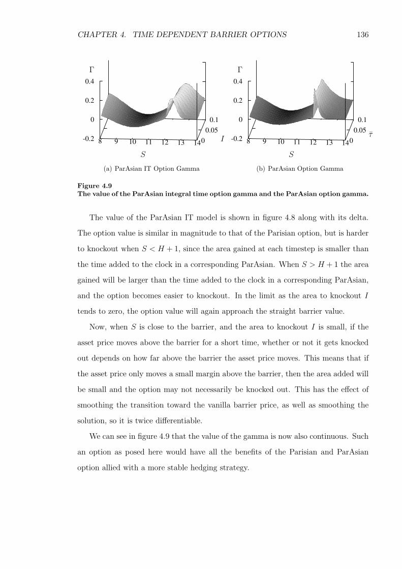
CHAPTER 4. TIME DEPENDENT BARRIER OPTIONS 136
8 9 10 11 12 13 14
0.1
0.05
0
0.2
0
-0.2
0.4
Γ
S
I
(a) ParAsian IT Option Gamma
8 9 10 11 12 13 14
0.1
0.05
0
0.2
0
-0.2
0.4
Γ
S
τ
(b) ParAsian Option Gamma
Figure 4.9The value of the ParAsian integral time option gamma and the ParAsian option gamma.
The value of the ParAsian IT model is shown in figure 4.8 along with its delta.
The option value is similar in magnitude to that of the Parisian option, but is harder
to knockout when S < H + 1, since the area gained at each timestep is smaller than
the time added to the clock in a corresponding ParAsian. When S > H + 1 the area
gained will be larger than the time added to the clock in a corresponding ParAsian,
and the option becomes easier to knockout. In the limit as the area to knockout I
tends to zero, the option value will again approach the straight barrier value.
Now, when S is close to the barrier, and the area to knockout I is small, if the
asset price moves above the barrier for a short time, whether or not it gets knocked
out depends on how far above the barrier the asset price moves. This means that if
the asset price only moves a small margin above the barrier, then the area added will
be small and the option may not necessarily be knocked out. This has the effect of
smoothing the transition toward the vanilla barrier price, as well as smoothing the
solution, so it is twice differentiable.
We can see in figure 4.9 that the value of the gamma is now also continuous. Such
an option as posed here would have all the benefits of the Parisian and ParAsian
option allied with a more stable hedging strategy.
CHAPTER 4. TIME DEPENDENT BARRIER OPTIONS 137
4.6 Conclusions
In this chapter we have examined some of the difficulties of using a Crank-Nicolson
scheme to price occupation-time derivatives. One of the main drawbacks, due to the
sharp changes in asset price with respect to the barrier time, is the large coefficient
of the O(∆t2) errors. When pricing time-dependent barrier options, similar problems
can be overcome by reducing the size of the timesteps near the implementation of the
barrier. However, we are constrained to keep our timesteps in both directions equal,
in order to stop oscillations in the solution. One possible way to circumvent this
may be to solve the two coupled PDEs, as suggested in Avellaneda and Wu (1999)
with different grids above and below the barrier. A more refined grid could be used
beyond the barrier to better capture the fast changing prices in this region. Another
method may be to apply singular perturbation analysis, again on the two coupled
PDEs; both of these avenues are left for further research.
Chapter 5
Modelling Bankruptcy with
ParAsian Options
In this chapter we consider the model developed in collaboration with Yu (2004)1.
The model uses ParAsian style options discussed in chapter 4. First, we will explain
the model, in which some minor modifications have been made by the author since the
original work of Yu (2004). Secondly, a description is given of the numerical methods
used to solve the problem along with some of the difficulties faced. Finally, a review
of results from the modified model will be given (from a mathematical perspective).
In developing the BSM model both Black and Scholes (1973) and Merton (1973)
recognised the potential for valuing corporate liabilities under the option pricing
framework. Now referred to as Merton-style bond pricing, or a structural model,
Merton (1974) values the default risk on a bond as a put option on the value of
the firm. The Yu (2004) model of bankruptcy using ParAsian options extends the
Merton-style pricing framework to include two important features. First, it can model
the accretion of debt by a firm as a constant factor over the life of the contract, by
a simple modification of the boundary conditions. Second, the model can include
violations of the absolute priority rule (APR) in a two-class debt structure. The
APR simply states that the senior creditors claims take precedence over the junior
1The model and results here are distinct from the original model by Yu. The chapter is looselybased on Yu et al. (2007) currently in preparation.
138
CHAPTER 5. MODELLING BANKRUPTCY WITH PARASIAN OPTIONS 139
creditors, and the junior creditors claims take precedence over the shareholders’ claims
in the event of default. The ParAsian feature allows the manner in which the creditors
are paid to be different at different times in the contract (specifically either before,
or at maturity), again just by modifying the boundary conditions. This means that
complex capital structure in the firm can now be modelled using Merton-style pricing.
The Yu (2004) model can also be used (by choosing the level of barrier with
respect to the total debt level) to mimic internal bargaining between the creditors,
and externally between the creditors and the debtors. The level of the barrier may
be chosen according to who is monitoring the firm, the senior creditors or their
subordinates, which will depend on their relative payoffs when the firm goes into
liquidation.
5.1 Literature
Hovakimian et al. (2001) give empirical evidence to suggest that a firm will ad-
here to a target leverage ratio, taking on new debt as the value of the firm increases,
although they also note that the initial target leverage ratio will change over time,
dependent on the firm’s profitability and stock price. In the usual structural model,
where the value of the firm is modelled by a log-normal geometric Brownian motion,
the leverage ratio will tend to zero as time tends to infinity. Collin-Dufresne and
Goldstein (2001) attempt to overcome this short-coming in Merton’s model by allow-
ing the accretion of debt to be a stochastic process in itself. They define a barrier,
kt, at which default occurs, which is the sum of the value of current debt and the
debt currently accrued. The process followed by kt is mean reverting to the target
financial policy of the firm. The model presented by Collin-Dufresne and Goldstein
(2001) is a reduced form model and requires the value of recovery rate to be specified,
whereas the Yu (2004) model has an endogenous recovery rate.
Of the structural models that have been derived from Merton (1974) innovative
work on corporate bonds, those such as Black and Cox (1976) and others give only
succinct details of the capital structure of the firm. However empirical evidence,
CHAPTER 5. MODELLING BANKRUPTCY WITH PARASIAN OPTIONS 140
such as that by Eom et al. (2004) suggests that to price bonds with a simple capital
structure will discount a large proportion of the bonds on the market. All of the
previous structural models assume that the APR is upheld in all instances, even
though there is strong evidence to the contrary. Since the APR is upheld, Black
and Cox (1976) show that, under their framework, the senior creditors always benefit
from the issuance of subordinate bonds as they increase the chances of the firm being
liquidated (the barrier for default is increased), while incurring all of the losses of the
creditors. Moraux (2003) uses a time-dependent barrier option, the Parisian, to price
debt, and shows how a two-class debt structure may be formed under his framework.
However the Yu (2004) model is superior in at least two ways. Parisian options are
inferior to ParAsian options when modelling bankruptcy, the creditors of the firm
will have a memory of the last time that the barrier was crossed, and will not be so
forgiving the next time, so the cumulative part of the option models the fact that if
the firm has been in distress, it is far more likely to be liquidated in the future. The
Parisian feature is included in Moraux (2003) by pricing a down-and-out call on the
firm value, where the value of debt is equal to the firm value short the down-and-out-
call. The subordinate bond is priced by going long in a down-and-out call with strike
price at senior level, and short a down-and-out call with strike price at the total debt
level. The barrier is placed at the total level of debt for all of the options. Under
Moraux’s framework, the fee received by the creditors cannot be altered to include
violation of the APR or the firm taking on new debt.
Both of the above structural models (Black and Cox, 1976; Moraux, 2003) assume
that the bonds mature at the same time. Geske (1977) was the first to price options
on options, or compound options, which can be applied to the Merton framework
of corporate bonds to price both coupon bonds, and bond issuances with different
maturity dates. To avoid difficulties with APR, Geske (1977), assumes that the senior
bond will always mature first, so that when pricing the subordinate debt, the senior
debt maturing is viewed as a coupon payment.
Using a reduced-form model, Unal et al. (2003) consider a two-debt structure
and allow for violations of the APR. To capture the violations of APR within the

CHAPTER 5. MODELLING BANKRUPTCY WITH PARASIAN OPTIONS 141
reduced-form framework, they must introduce a new parameter to model the extra
payment to the junior creditors when the APR is violated. This results in another
parameter which must be prescribed, along with the recovery rates, whereas they are
both endogenous to the Yu (2004) model.
Leland (1994) develops a model to find optimal leverage ratio for a firm subject
to default risk, tax, interest rate, bond covenants, payout ratio and the bankruptcy
costs. Using perpetual options and constant interest rates they can generate closed
form solutions. Here the default barrier is determined endogenously in the solution.
Later, Leland and Toft (1996) relax the perpetuity of the option to find the optimal
maturity of the bond issue. Ju and Ou-Yang (2006) extend the model further to
include stochastic interest rates and find that they have a large role to play in the
optimisation of capital structure. Broadie et al. (2007) also look to extend the Leland
(1994) model this time by including a renegotiation period. Although the probability
of default is increased, the probability of liquidation is now decreased implying that
the renegotiation period helps the recovery of firm in distress. They use a binomial
method outlined in Broadie and Kaya (2007) that can also be used on the Leland
(1994) model.
5.2 The Model
In this section we give a brief description of the Yu (2004) model. When there
is a two class debt structure, we can allow for earlier maturing debt by altering the
boundary conditions. By using similar methods to those outlined by Geske (1977),
we could price bonds with different maturities, but this could potentially lead to
infinite combinations of the two maturities. In order to produce the term structure
for the bonds for comparison, the bonds have the same maturity with one maturing
infinitesimally before the other.
Let us consider the Yu (2004) model with a single debt class. In the classic
Merton (1974) model, the bond holder is long the principal amount, and short a put
on the firm value with strike price equal to the principal amount. Black and Cox

CHAPTER 5. MODELLING BANKRUPTCY WITH PARASIAN OPTIONS 142
(1976) introduce a safety covenant in the form of a straight knockout barrier (with
rebate), and the Yu model takes this barrier and allows the firm value to be below the
barrier for a predetermined amount of time, while the firm undergoes chapter 112,
which in this context, we shall call the window. The window attempts to capture
the renegotiation of the firm over the lifetime of the bond. Hotchkiss (1995) and
Gilson (1997) find that a large proportion of firms that have undergone renegotiation
will perform badly and are likely to enter into reorganisation again, meaning that a
cumulative time spent in reorganisation is more appropriate than consecutive time:
the creditors will be less forgiving if the firm has been recently in distress. The value
of the barrier depends on how closely the creditors monitor the firm. There must
be some trade-off, between the cost of monitoring the firm, which is an expensive
process (Rajan and Winton, 1995), and the potential losses to the creditors. With a
ParAsian option, the barrier may be placed at the level of the debt, which has a trivial
value for the straight barrier model (if the safety covenant is at the debt level, the
creditors instantly default the firm if the bond cannot be repaid, will incur no losses
and the bond is risk-free), or even above it without trivial results. If the creditors
act optimally (ignoring the cost of monitoring) then they will place the barrier at the
level of debt.
When the debt is divided into two classes, Yu (2004) argues that there is an
internal bargaining between the creditors that drives the positioning of the barrier.
If the junior creditors cooperate with the senior bond holders, then they will take on
the monitoring of the firm and the barrier is placed at the total debt level. If they
choose not to cooperate, they may leave the monitoring to the senior creditors, in
which case the barrier is placed at the senior debt level. In the results section we
present the credit spread for a full range of barrier levels.
When firms issue debt, the senior bonds will often have covenants to safeguard the
priority of their debt over earlier-maturing debt. Such a covenant is the cross-default
provision, whereby the senior debt is automatically defaulted if the subordinate bond
defaults, maintaining priority for the senior debt. Defining S as the face value of
2Chapter 11 is a form of bankruptcy that allows reorganisation of the companies debt obligations.

CHAPTER 5. MODELLING BANKRUPTCY WITH PARASIAN OPTIONS 143
0
20
40
60
80
100
0 50 100 150 200
Bo
nd
Val
ue
(S/J
)
Firm Value (V)
(a)
0
20
40
60
80
100
0 50 100 150 200
Bo
nd
Val
ue
(S/J
)
Firm Value (V)
(b)
Figure 5.1Payoffs to Junior and Senior Debt Issues When Junior Debt Matures First.(a) Junior debt has a higher proportion of the total debt; with S = 20 (solid line) and J = 80
(dotted line). (b) Senior debt with a higher proportion of total debt; S = 80 (solid line) and J = 20
(dotted line).
senior debt, and J as the face value of junior debt, figures 5.1(a) and 5.1(b) show
the payoff at maturity to the senior and junior debt holders when the junior debt
matures first. The senior debt does not always maintain priority even with the cross-
default provision. These figures form the basis for our final conditions for the bonds
at maturity.
5.3 The Valuation Framework
5.3.1 Assumptions
The cooperative models for the case when senior debt matures earlier and the
case when senior debt matures later are labelled as Models Ia and Ib respectively.
The non-cooperation model is labelled as Model II, and is applicable to both matu-
rity structures (corresponding to Models Ia and Ib), but with a different bargaining
condition; for a single debt issue, we use Model Ia with the face value of junior debt
equal to zero, however, the basic assumptions of the models are the same:
Firm value : The dynamics for the asset value, V , follow a geometric Brownian

CHAPTER 5. MODELLING BANKRUPTCY WITH PARASIAN OPTIONS 144
motion
dV =
[
µ V − δ(t− tcs)cs2St−cs− δ(t− tcj
)cj2Jt−cj
− δ(t− td)d
2(V − St−d
− Jt−d)+
]
dt+ σV V dZV , (5.1)
where µ is the instantaneous expected rate of return on the firm, δ(·) is the
Dirac delta function, cs, cj and d are coupon rates for senior and junior debt
and dividend yield, paid semi-annually at tcs, tcjand td, respectively, σV is the
volatility of the asset, dZV is a standard Gauss-Wiener process. Here St− and
Jt− represent the total face value of debt in the firm that is senior and junior
respectively (including newly issued debt here). Since the dividend is paid to
equity holders, the amount paid is proportional to the firm value minus the face
value of debt, or zero if the firm value is below the face value of debt.
Risk-free interest rate : The dynamics of the instantaneous risk-free interest rate,
r, follow the Cox et al. (1985) model:
dr = κ(θ − r)dt+ σr
√rdZr, (5.2)
where κ is the speed of a mean-reverting process for the short rate; θ is the
long-run mean level of interest rate; σr is the volatility parameter; dZr is also
a standard Gauss-Wiener process. The instantaneous correlation coefficient
between these two Gauss-Wiener processes is ρ:
E[dZV dZr] = ρdt.
Recovery :
In contrast to normal structural models where the level of the barrier is in
some sense equivalent to the recovery rate, the recovery rate in the ParAsian

CHAPTER 5. MODELLING BANKRUPTCY WITH PARASIAN OPTIONS 145
framework is endogenous to the model, and so the ParAsian barrier is placed
at the total value of the debt. Hence we are not required to give an explicit
value for the recovery rate. However at the end of the window, we must decide
whether the face value of the bond must be paid in cash, or equivalent securities
paying face value at maturity. In most reduced form models such as Longstaff
and Schwartz (1995), the recovery rate is defined as the “the fraction of the
present value of an otherwise equivalent Treasury bond”, and we adopt this
approach so that the payout at the end of the window is a security paying
face value at maturity. Although there is some evidence to suggest that the
recovery rate is best described as “the fraction of the face value of the debt”,
RFV (Guha, 2002), this could cause some complications. It could be possible
for the bond to default even when the firm is not distressed (if interest rates are
very high, the value of the firm could be below the face value of the debt, but
above the market value), and the bondholders receive more than the bond is
worth on the market. This would result in negative credit spreads and possibly
negative duration.
Debt level and leverage ratio :
In our model the firm adheres to a constant target leverage ratio. In other
words, the firm takes on new debt at the rate at which the total value of
the firm increases, in order to keep leverage constant. Under the risk-neutral
measure, the rate at which the value of the firm increases is the current interest
rate. Then we model the drift of debt level as partly dependent on interest rates
(in a risk-neutral environment, the long term mean level of the interest rate θ
is the best approximation), and partly dependent on the firm’s payout policy.
If we let ζ denote the annual payout ratio by the firm, it can be summarised as
ζV = cs′ · Senior Debt + cj
′ · Junior Debt + d′ · Equity,
where cs′, cj
′ and d′ are the coupons and dividends annualised at a continuous
CHAPTER 5. MODELLING BANKRUPTCY WITH PARASIAN OPTIONS 146
rate. The current total face value of debt at time t can be expressed as:
F (t) = F0 eφt,
where F0 is the initial face value of total debt, and φ = θ − ζ is the capital
accumulation factor. However, since interest rates are treated as stochastic, the
level of the barrier should depend not only on the face value of the debt, but
also on the interest rate. Let Lc(t, r;T ) be the market value of an equivalent
risk-free coupon bond paying 1 dollar at maturity T , with the same coupon
payment setting as our corporate bond. This bond can be priced using the CIR
equation. Then the default barrier value K(t, r) at time t is set to be:
K(t, r) = F0 · eφt · Lc(t, r;T ). (5.3)
Equation (5.3) is consistent with the definition of recovery rate as the fraction
of the equivalent Treasury bond. If we take the recovery rate to be RFV, then
the barrier will be:
K(t, r) = F0 · eφt. (5.4)
ParAsian feature : The trigger of default in the time dimension is the window
length of ParAsian options, T . In addition, when the firm is worthless, it be-
comes futile in any model for creditors to continue to wait for the emergence of
the firm. Zero asset value becomes an absorbing barrier; the window automat-
ically reaches its end for any t, the measure of the cumulative time below the
default barrier. The dynamics of the ParAsian feature follow those set down in
chapter 4:
dt =
0 if V > K(t, r),
dt otherwise.

CHAPTER 5. MODELLING BANKRUPTCY WITH PARASIAN OPTIONS 147
5.3.2 Partial differential equation - derivation
Pricing the risky debt requires the solution of a four-dimensional problem (in t,
t, V and r). The partial differential equations (PDEs) for both senior and junior
debt are the same as for a single issue, in that they are derived from a common
process of firm value and interest rates. They differ from one another only through
the terminal conditions. Let L denote an otherwise risk-free bond; if we construct
a portfolio with long one bond and short a number (Dr/Lr) of risk-free bonds (to
eliminate interest-rate risk) and short a number (DV ) of the underlying asset (to
eliminate asset risk), then by applying Ito’s lemma to equations (5.1) and (5.2), the
no-arbitrage condition to the portfolio value (see Yu, 2004 for a full derivation), we
obtain the partial differential equation:
Dt +Dt +1
2DV V σ
2V V
2 +1
2Drrσ
2rr +DV rσV V σr
√rρ
+Dr
(
κ(θ − r)− λσr
√r)
+ rDV = rD, (5.5)
where λ is the market price of risk and D is the general term for debt, which can be
senior debt, B, or junior debt, b, or the former definition as the total debt; subscripts
on D denote partial derivatives.
At the coupon and dividend dates, the value of the debt must satisfy
D(V+, r, t, t+) = D(V−, r, t, t−), (5.6)
where
V+ = V− −cs2Seφt − cj
2Jeφt − d
2max(V− − Seφt − Jeφt, 0). (5.7)
The value of the debt just after a dividend payment is found by interpolation.
5.3.3 Boundary conditions
The ParAsian features are realised in the boundary conditions, which are required
to solve the partial differential equation above.

CHAPTER 5. MODELLING BANKRUPTCY WITH PARASIAN OPTIONS 148
At maturity (terminal condition 1) : When the junior and senior debts mature
at different times, the later debt maturity initially appears to be a better choice,
but the earlier maturity must be specified and incorporated beforehand, which
implies unlimited combinations. The boundary condition at maturity must take
into account the issue of new debt, which we assume to be of equal priority to
current debt (Smith and Warner, 1979; Fama and Miller, 1972) and issued in
such a way so as to maintain the ratio of senior to junior debt. As a result, when
the firm defaults, the creditors must share their claim with the new creditors. In
the original model proposed by Yu (2004), the debt in its entirety was included
at the terminal condition, however the original creditors have no claim on newly
issued debt. If we let the face value of the new debt issued be, say, N , and
S = aF0, J = (1− a)F0 be the face value of original debt where the parameter
a defines the proportion of senior debt in the total debt, then aN is senior debt
and (1− a)N is junior debt. Consequently, the senior debt at default will be
B = min[ V SS+aN
, S]
= min[ V aDaD+aN
, S]
= min[ V DD+N
, S]
= min[ V DDeφT , S]
= min[V e−φT , S]. (5.8)
Therefore, at its expiration for any τ ≤ T , the payoffs of debt in Model Ia and
Ib are:
B(T, V, r, τ) = Min[V (T ) · e−φT , S],
b(T, V, r, τ) = Min[Max[V (T ) · e−φT − S, 0], J ];
the payoffs in Model II are:
B(T, V, r, τ) =
Min[V (T ) · e−φT − J, S] if V (T ) ≥ J · eφT
Min[V (T ) · e−φT , S] otherwise,

CHAPTER 5. MODELLING BANKRUPTCY WITH PARASIAN OPTIONS 149
b(T, V, r, τ) =
Min[V (T ) · e−φT , J ] if V (T ) ≥ J · eφT
Min[Max[V (T ) · e−φT − S, 0], J ] otherwise.
At the end of the window (terminal condition 2) : Whenever the ParAsian
feature is realised, in all models, creditors seize the firm and realise payoffs
according to the APR, again Lc(t, r;T ) is the market value of an equivalent
risk-free coupon bond paying 1 dollar at maturity T :
B(t, V, r, T ) = Min[V (t) · e−φt, S · Lc(t, r;T )],
b(t, V, r, T ) = Min[Max[V (t) · e−φt − S · Lc(t, r;T ), 0], J · Lc(t, r;T )].
Asset value is zero : When the firm has no value, all its securities are worthless:
B(t, 0, r, τ) = b(t, 0, r, τ) = 0.
Asset value is infinite : Under these circumstances, creditors are guaranteed their
claims without suffering loss:
B(t,∞, r, τ) = S · Lc(t, r;T ),
b(t,∞, r, τ) = J · Lc(t, r;T ).
Interest rate is zero : When the interest rate is zero, according to the CIR model,
the interest rate at the next instant is κθdt with certainty (since σr
√rdZr = 0).

CHAPTER 5. MODELLING BANKRUPTCY WITH PARASIAN OPTIONS 150
The PDE reduces to
Dt +1
2DV V σ
2V V
2 +Drκθ +Dτ = 0.
(d‘Halluin et al., 2001 showed that for the CIR model this PDE does not require
a boundary condition at r = 0, so long as the condition that the Feller, 1951
condition 2κθ/σ2r ≥ 1 is satisfied)
Interest rate is infinite: When the interest rate is infinite, the present value of
any asset, becomes zero:
B(t, V,∞, τ) = b(t, V,∞, τ) = 0.
5.3.4 Parameter choices
The numerical examples produced in Yu (2004), and here, borrow the “empirically
reasonable parameter choices” in Huang and Huang (2003). In contrast, Longstaff
et al. (2005) employ the new information available from credit default swap data to
determine the default component accounts for the majority of corporate bond spread
across all credit ratings (Blanco et al., 2005; Driessen, 2005). The yield spreads gen-
erated herein are effectively credit spreads. Our results are not directly comparable
with those of Huang and Huang (2003), as recovery rate and default boundary level
are important parameter choices. Nevertheless, it is interesting to note that the sizes
of credit spreads generated in this chapter match the ideal scenario in Huang and
Huang (2003).3
Calibrated with the same economic assumptions as those in Huang and Huang
(2003), our parameter choices are: the initial value of total debt F = 100, (Huang and
Huang, 2003 assume that bonds are issued at par), which we arbitrarily decompose
into S = 20 and J = 80 or S = 80 and J = 20 in pairs to examine the effect
3The results in the next section are different, although similar, from those presented in Yu (2004),all computer codes were written and run by the author of this thesis for both sets of results.

CHAPTER 5. MODELLING BANKRUPTCY WITH PARASIAN OPTIONS 151
Table 5.1Leverage Ratio and Asset Volatility For Each Rating
Aaa Aa A Baa Ba B C D
Leverage ratio(%)
13.1 21.2 32.0 43.3 53.5 65.7 100.0 125.0
Asset Volatility(%)
36.6 34.8 30.0 29.1 34.3 39.3 45.0 50.0
of relative weights of the two classes; the leverage ratio and the volatility of asset
value σV depend on the firm’s specific feature (a proxy here is the credit rating)
and are listed in Table 5.1, the credit ratings following Moody’s system; the annual
coupon rate cs = cj = 8.162%; the annual asset payout ratio ζ = 6%; the initial
instantaneous rate r0 = 8%; mean reverting speed κ = 0.226; long-term mean level
of interest rate θ = 0.113; volatility parameter σr = 4.68%; the market price of risk
λ = 0; the correlation coefficient between asset return and the change in interest
rate ρ = −0.25. For the window time, T , Yu (2004) cites values from Eberhart and
Sweeney (1992), that the average time in reorganisation is 25.6 months (2.1 years);
and Altman (1993), that the reorganisation experience on average is 21 months, and
so we set T = 2 years.
5.4 Numerical Method
Following the analysis detailed in chapters 3 and 4, for multi-asset options, and
time-dependent barrier options, we must now combine the two. We make the usual
substitutions, defining τ and τ , such that
0 < τ = T − t < T, 0 < τ = T − t < T .
Then applying this change of variables to (5.5) we have the following PDE,
Dτ +Dτ =1
2DV V σ
2V V
2 +1
2Drrσ
2rr +DV rσV V σr
√rρ
+Dr
(
κ(θ − r)− λσr
√r)
+ rDV − rD. (5.9)

CHAPTER 5. MODELLING BANKRUPTCY WITH PARASIAN OPTIONS 152
From the analysis on time-dependent barrier options in chapter 4 (see particularly
section 4.4) we deduce that the problem must be approached differently depending on
the terminal conditions. When pricing within a single debt structure, or in a two class
debt structure with APR upheld, the terminal conditions at expiry and knockout are
continuous. This means that the most appropriate manner to discretise is with a
Crank-Nicolson style scheme setting the timesteps in real time equal to the barrier
timesteps. However, when the APR is not upheld in a two-class debt structure, the
Crank-Nicolson scheme will be prone to ringing and an implicit scheme must be used.
∆τ =
∆t if V ≤ Kr,t
0 if V > Kr,t .
We next define the value of debt at a particular point to be
D(V, r, t, τ) = D(i ·∆V, j ·∆r, k ·∆t, l ·∆τ) = Dk,li,j
As a result, the left-hand side of (5.9) can now be written
Dt +Dτ =
1∆t
(Dk+1,l+1i,j −Dk,l
i,j ) if V ≤ Kr,t
1∆t
(Dk+1,l+1i,j −Dk,l+1
i,j ) if V > Kr,t
. (5.10)
Since we are now working with an extra dimension (interest rate), the barrier is
a line rather than the usual point barrier synonymous with other models. Now the
barrier is chosen to be the total face value multiplied by the value of an equivalent
Treasury bond, hence we must find the value of the treasury bond Lc a priori since
it is a function of both time and interest rate. The Treasury bond value can either be
found using a finite-difference scheme on the CIR equation, or we may take advantage
of the fact that there is an analytical solution4 available. We choose the latter, then
4A closed-form formula for a risk-free bond with initial interest rate r is:
P (r, T ) = H(T )e−G(T )r,
with
H(T ) =[ 2γ e(κ+λ+γ)T/2
(κ + λ + γ)(eγτ − 1) + 2γ
]2κθ/σ2
,

CHAPTER 5. MODELLING BANKRUPTCY WITH PARASIAN OPTIONS 153
assume that Lc is now a known function, then the barrier value may be expressed as
hkj = INT
(
F eφtk Lc(tk, rj)
∆V
)
+ 1 (5.11)
where hkj is the integer equivalent to Kr,t. By definition of the function ‘INT’, hk
j ≤
Kr,t, so if i ≤ hkj then the node (i, j) is below or at the barrier.
Now, after expanding each of the terms in (5.9), a set of equations of the following
form is obtained for Dk+1,l+1i,j ,
αi,jDk+1,l+1i−1,j + βi,jD
k+1,l+1i,j + γi,jD
k+1,l+1i+1,j
+δi,jDk+1,l+1i,j−1 + ǫi,jD
k+1,l+1i,j+1
+µi,j(Dk+1,l+1i−1,j−1 −Dk+1,l+1
i−1,j+1 +Dk+1,l+1i+1,j+1 −Dk+1,l+1
i+1,j−1) = Zi,j (5.12)
for 0 < i < n and 0 < j < m, where the right-hand-side of the equation is
Zi,j = αi,jDk,li−1,j + βi,jD
k,li,j + γi,jD
k,li+1,j + δi,jD
k,li,j−1 + ǫi,jD
k,li,j+1
+µi,j(Dk,li−1,j−1 −Dk,l
i−1,j+1 +Dk,li+1,j+1 −Dk,l
i+1,j−1) if i ≤ hkj
Zi,j = αi,jDk,l+1i−1,j + βi,jD
k,l+1i,j + γi,jD
k,l+1i+1,j + δi,jD
k,l+1i,j−1 + ǫi,jD
k,l+1i,j+1
+µi,j(Dk,l+1i−1,j−1 −Dk,l+1
i−1,j+1 +Dk,l+1i+1,j+1 −Dk,l+1
i+1,j−1). if i > hkj
This scheme is implicit and we are presented with a (m+1).(n+1)× (m+1).(n+1)
matrix system to compute.
Next, we must decide how to solve this set of equations in a fast and efficient way.
We are presented with two issues. First, at each barrier time step we have to solve a
two-dimensional PDE problem. Second, the storage space required is extremely large
as we are solving for a three-dimensional array, which is dependent on the number of
timesteps. In fact, when we double the timesteps, not only will we double the storage
G(T ) =2(eγτ − 1)
(κ + λ + γ)(eγτ − 1) + 2γ,
andγ =
√
(κ + λ)2 + 2σ2,
where λ is the market price of interest rate risk (Cox et al., 1985).

CHAPTER 5. MODELLING BANKRUPTCY WITH PARASIAN OPTIONS 154
requirements, but also the number of discretised solutions to be solved.
We decided that the ideal method would be to solve the entire set of equations
simultaneously using the (sparse) banded routine in the NAG library. This way, we
did not need to consider any stability issues of the method, as we can obtain an
‘exact’ solution to the above set of equations. However, if were to use this method to
solve over the range τ ∈ [0, T ] at each timestep, the code is slow and laborious. When
solving (for example) a ten year bond, the number of timesteps used becomes very
important so as to maintain accuracy in the solution. With this method, doubling
the number of timesteps will, in fact, quadruple (at the very least) the computation
time.
The direct sparse solver is preferable to schemes based on iteration (e.g. point or
line relaxation) in regions where the solution changes rapidly; however, as we solve
over the range τ ∈ [0, T ], the solution will tend toward a constant European value
as τ increases. In fact, if τ > t then the solution is European and Dl+1 = Dl. It
is obvious that it would be inefficient to use the sparse solver in the region τ > t
when we have already calculated the solution, but if we inspect figure 5.4 we see
that there is a significant region in [0, T ] over which the solution is approximately
constant. Iterating to find the solution in this region should be expected to be quick
to converge if we use an iterative scheme with the solution at k as our initial guess.
Hence, we use a successive over relaxation scheme in conjunction with the sparse
solver. Thus, combining the two schemes is more efficient than using either on its
own, because increasing the number of time steps will improve the accuracy of the
initial guess for the next solution and, hence, the required number of iterations will
decrease. Even though the required number of calculations has increased 4-fold, in
practice the computation time only increases by a factor of between 2 and 3.
Table 5.2 documents the convergence of the Crank-Nicolson scheme used for single
class debt calculations in this chapter. As in chapter ??, the solution exhibits linear
convergence, and the Richard extrapolated solution shows quadratic convergence,
allowing for further extrapolation of the results. We see that the twice extrapolated
results give sufficient accuracy to price the credit risk to the nearest basis point.

CHAPTER 5. MODELLING BANKRUPTCY WITH PARASIAN OPTIONS 155
Table 5.2Convergence of the bond price
n m p D(V0, r0, 0, 0) DRE DRE2 Credit Spread (bps)
51 5 9 76.8761101 9 17 77.0074 77.1387201 17 33 77.0704 77.1335 77.1317 505.8401 33 65 77.1071 77.1437 77.1471 505.4801 65 129 77.1274 77.1478 77.1492 505.31601 129 257 77.1383 77.1491 77.1496 505.2
A table showing the convergence of the Crank-Nicolson method. We price a 5 year B-rated bond
in a single debt structure with parameters as defined in section 5.3.4, at the given firm value V0
and interest rate r0. n, m and p are the number of points in V , r and t respectively. The grid is
contained by V ∈ [0 : 5F ], r ∈ [0 : 4r0] and t ∈ [0, 2]. The value of the straight calculation is shown
in the fourth column, with once and then twice extrapolated results (Richardson extrapolation, see
chapter 4) in the fifth and sixth columns respectively. The price of the equivalent treasury bond is
95.0388, and the final column shows the credit spread of the twice extrapolated results.
Here, since we are investingating the general shape and qualitative effects of the
model, pricing to the nearest basis point is all that is required.
5.5 Results for a Single Class of Debt
We will show first the features arising from our ParAsian model with a single debt
class. The window length in the model will be seen to influence both the level and
the shape of the term structure of credit spreads. The influence of interest rate, its
volatility, and other factors in the model will be discussed.
5.5.1 Credit Spread and Firm Rating
In order to relate results here conveniently to observed shapes and trends in bond
data, a proxy is required for the ratings given by the major agencies, such as Moodys,
Standard & Poor’s, Fitch and others. Clearly, this is an imprecise science; practical
bond ratings are not determined by a single, simple factor, but we will follow in the
footsteps of Merton (1974), who used the quasi-leverage ratio as a reasonable proxy,
to demonstrate general features. Having already used their key data inputs, we
again follow Huang and Huang (2003) in relating leverage ratios to Moodys ratings.
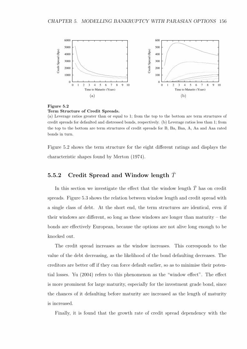
CHAPTER 5. MODELLING BANKRUPTCY WITH PARASIAN OPTIONS 156
0
1000
2000
3000
4000
5000
6000
0 1 2 3 4 5 6 7 8 9 10
Cre
dit
Sp
read
(B
ps)
Time to Maturity (Years)
(a)
0
100
200
300
400
500
600
0 1 2 3 4 5 6 7 8 9 10
Cre
dit
Sp
read
(B
ps)
Time to Maturity (Years)
(b)
Figure 5.2Term Structure of Credit Spreads.(a) Leverage ratios greater than or equal to 1; from the top to the bottom are term structures of
credit spreads for defaulted and distressed bonds, respectively. (b) Leverage ratios less than 1; from
the top to the bottom are term structures of credit spreads for B, Ba, Baa, A, Aa and Aaa rated
bonds in turn.
Figure 5.2 shows the term structure for the eight different ratings and displays the
characteristic shapes found by Merton (1974).
5.5.2 Credit Spread and Window length T
In this section we investigate the effect that the window length T has on credit
spreads. Figure 5.3 shows the relation between window length and credit spread with
a single class of debt. At the short end, the term structures are identical, even if
their windows are different, so long as these windows are longer than maturity – the
bonds are effectively European, because the options are not alive long enough to be
knocked out.
The credit spread increases as the window increases. This corresponds to the
value of the debt decreasing, as the likelihood of the bond defaulting decreases. The
creditors are better off if they can force default earlier, so as to minimise their poten-
tial losses. Yu (2004) refers to this phenomenon as the “window effect”. The effect
is more prominent for large maturity, especially for the investment grade bond, since
the chances of it defaulting before maturity are increased as the length of maturity
is increased.
Finally, it is found that the growth rate of credit spread dependency with the
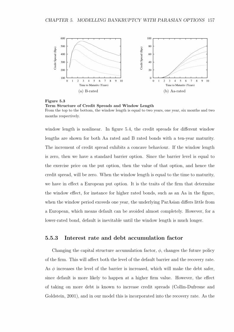
CHAPTER 5. MODELLING BANKRUPTCY WITH PARASIAN OPTIONS 157
100
200
300
400
500
600
0 1 2 3 4 5 6 7 8 9 10
Cre
dit
Sp
read
(B
ps)
Time to Maturity (Years)
(a) B-rated
0
20
40
60
80
100
0 1 2 3 4 5 6 7 8 9 10
Cre
dit
Sp
read
(B
ps)
Time to Maturity (Years)
(b) Aa-rated
Figure 5.3Term Structure of Credit Spreads and Window LengthFrom the top to the bottom, the window length is equal to two years, one year, six months and two
months respectively.
window length is nonlinear. In figure 5.4, the credit spreads for different window
lengths are shown for both Aa rated and B rated bonds with a ten-year maturity.
The increment of credit spread exhibits a concave behaviour. If the window length
is zero, then we have a standard barrier option. Since the barrier level is equal to
the exercise price on the put option, then the value of that option, and hence the
credit spread, will be zero. When the window length is equal to the time to maturity,
we have in effect a European put option. It is the traits of the firm that determine
the window effect, for instance for higher rated bonds, such as an Aa in the figure,
when the window period exceeds one year, the underlying ParAsian differs little from
a European, which means default can be avoided almost completely. However, for a
lower-rated bond, default is inevitable until the window length is much longer.
5.5.3 Interest rate and debt accumulation factor
Changing the capital structure accumulation factor, φ, changes the future policy
of the firm. This will affect both the level of the default barrier and the recovery rate.
As φ increases the level of the barrier is increased, which will make the debt safer,
since default is more likely to happen at a higher firm value. However, the effect
of taking on more debt is known to increase credit spreads (Collin-Dufresne and
Goldstein, 2001), and in our model this is incorporated into the recovery rate. As the

CHAPTER 5. MODELLING BANKRUPTCY WITH PARASIAN OPTIONS 158
0
100
200
300
400
500
600
0 2 4 6 8 10
Cre
dit
Sp
read
(B
ps)
Window Length (Years)
(a) B-rated
0
20
40
60
80
100
0 2 4 6 8 10
Cre
dit
Sp
read
(B
ps)
Window Length (Years)
(b) Aa-rated
Figure 5.4Credit Spread vs. Window LengthCredit spread for a ten year bond with varying window length. Parameters are as given in the text.
200
300
400
500
0 1 2 3 4 5 6 7 8 9 10
Maturity T
Cre
dit
Spre
ad
(bps)
(a) φ = 0
200
300
400
500
0 1 2 3 4 5 6 7 8 9 10
Maturity T
Cre
dit
Spre
ad
(bps)
(b) φ = r − ζ
Figure 5.5Term structure for varying interest rate in a one-factor model(a) The rate at which the firm accumulates debt is held constant with φ = 0, and the constant
interest rate is varied from r = 6% (solid) through to r = 12% (dotted). (b) The rate at which the
firm accumulates debt is matched to the interest rate, φ = r − ζ, and the constant interest rate is
varied from r = 6% (solid) through to r = 12% (dotted).
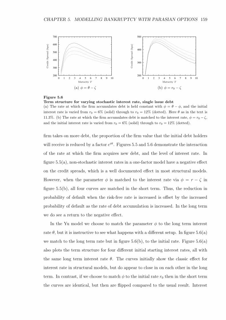
CHAPTER 5. MODELLING BANKRUPTCY WITH PARASIAN OPTIONS 159
200
300
400
500
600
700
0 1 2 3 4 5 6 7 8 9 10
Maturity T
Cre
dit
Spre
ad
(bps)
(a) φ = θ − ζ
200
300
400
500
0 1 2 3 4 5 6 7 8 9 10
Maturity T
Cre
dit
Spre
ad
(bps)
(b) φ = r0 − ζ
Figure 5.6Term structure for varying stochastic interest rate, single issue debt(a) The rate at which the firm accumulates debt is held constant with φ = θ − φ, and the initial
interest rate is varied from r0 = 6% (solid) through to r0 = 12% (dotted). Here θ as in the text is
11.3%. (b) The rate at which the firm accumulates debt is matched to the interest rate, φ = r0− ζ,
and the initial interest rate is varied from r0 = 6% (solid) through to r0 = 12% (dotted).
firm takes on more debt, the proportion of the firm value that the initial debt holders
will receive is reduced by a factor eφt. Figures 5.5 and 5.6 demonstrate the interaction
of the rate at which the firm acquires new debt, and the level of interest rate. In
figure 5.5(a), non-stochastic interest rates in a one-factor model have a negative effect
on the credit spreads, which is a well documented effect in most structural models.
However, when the parameter φ is matched to the interest rate via φ = r − ζ in
figure 5.5(b), all four curves are matched in the short term. Thus, the reduction in
probability of default when the risk-free rate is increased is offset by the increased
probability of default as the rate of debt accumulation is increased. In the long term
we do see a return to the negative effect.
In the Yu model we choose to match the parameter φ to the long term interest
rate θ, but it is instructive to see what happens with a different setup. In figure 5.6(a)
we match to the long term rate but in figure 5.6(b), to the initial rate. Figure 5.6(a)
also plots the term structure for four different initial starting interest rates, all with
the same long term interest rate θ. The curves initially show the classic effect for
interest rate in structural models, but do appear to close in on each other in the long
term. In contrast, if we choose to match φ to the initial rate r0 then in the short term
the curves are identical, but then are flipped compared to the usual result. Interest

CHAPTER 5. MODELLING BANKRUPTCY WITH PARASIAN OPTIONS 160
rates (combined with φ) now have a positive effect on the credit spreads. Hence, the
influence of the parameter φ outweighs the effects of the interest rate.
In this chapter, to allow comparisons to be made, we choose the parameter φ to
be constant across all firm ratings. However, it may be better to vary this parameter
according to the firm rating, and hence the probability with which it will take on new
debt. This implies φ will be relatively small for speculative grade bonds, and high
for investment grade bonds. We can then reproduce the results of Collin-Dufresne
(2001) in which the credit spreads will be less variable across firm ratings.
5.5.4 Duration
It is well documented that defaultable bonds have shorter durations than equiv-
alent risk-free bonds (Chance, 1990; Longstaff and Schwartz, 1995). Here, the most
common definition of duration is adopted, namely the negative percentage change
in bond price to the change in its own yield (an alternative definition adopted by
Acharya and Carpenter, 2002 is a ratio to the change in a corresponding T-bond
yield). Figure 5.7(a) illustrates duration decreasing with the increase in default risk.
Under the Yu framework, negative durations are not possible, even for very high risk
bonds. Longstaff and Schwartz (1995) present a set of parameters (the bond is close
to default and the recovery rate is low) for which bond price increases as interest
rates are increased, resulting in negative duration, which agrees with the conditions
required for negative duration argued by Acharya and Carpenter (2002). Although
the default barrier is similar in both the Yu (2004) model and the Longstaff and
Schwartz (1995) model, in as much as an increase in interest rates can reduce the
probability of hitting the barrier (both barriers are decreasing functions of interest
rate), the endogenous nature of recovery in the Yu model means that there is no loss
avoided by such a movement: hitting the barrier does not result in a loss. Therefore
with endogenous recovery rate, no negative durations are possible.
In figure 5.7(b), the effect of window length on the duration of the bond is shown.
The window length gives us an indication of the riskiness of a bond, with short

CHAPTER 5. MODELLING BANKRUPTCY WITH PARASIAN OPTIONS 161
5.6
5.8
6
6.2
6.4
6.6
6.8
7
AaaAaABaaBaBdistressdefault
Du
rati
on
(Y
ears
)
Firm Rating
(a) Firm Ratings vs. Duration
6.2
6.3
6.4
6.5
6.6
6.7
6.8
6.9
0 2 4 6 8 10
Du
rati
on
(Y
ears
)
Window Length (Years)
(b) Duration vs. Window Length; an Aa-ratedbond (dashed line) and a B-rated bond (solid line).
Figure 5.7Duration
windows the bond is almost riskless, and the risk increases as the window increases
and the creditors become less protected. As the window length tends toward zero,
both the speculative and investment grade bonds tend to the same riskfree duration
value. As mentioned before, it is well known that duration reduces with increased
risk so it is no surprise that duration reduces as the window is increased.
5.6 Results for a Two-Class Debt Structure
The scene has now been set for consideration of a two-class debt structure. In the
following examples, only results for B and Aa rated bonds are displayed, as examples
of speculative and investment grade bonds.
5.6.1 Credit spread and priority
Figure 5.8 compares the term structures of credit spreads generated in Model Ia
and those of two single issues whose face value is equivalent either to the total debt
level (i.e. the single debt structure) or to the senior debt level, fixing other parameters
in the same rated firm.
The results in figure 5.8 are standard, and are consistent with the findings in
Black and Cox (1976), where the senior debt is less risky than, and the junior debt
more risky than the combined total debt. Here the APR is upheld, so the junior debt
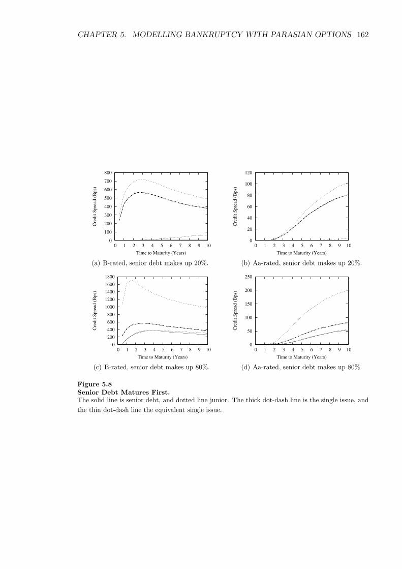
CHAPTER 5. MODELLING BANKRUPTCY WITH PARASIAN OPTIONS 162
0
100
200
300
400
500
600
700
800
0 1 2 3 4 5 6 7 8 9 10
Cre
dit
Sp
read
(B
ps)
Time to Maturity (Years)
(a) B-rated, senior debt makes up 20%.
0
20
40
60
80
100
120
0 1 2 3 4 5 6 7 8 9 10
Cre
dit
Sp
read
(B
ps)
Time to Maturity (Years)
(b) Aa-rated, senior debt makes up 20%.
0
200
400
600
800
1000
1200
1400
1600
1800
0 1 2 3 4 5 6 7 8 9 10
Cre
dit
Sp
read
(B
ps)
Time to Maturity (Years)
(c) B-rated, senior debt makes up 80%.
0
50
100
150
200
250
0 1 2 3 4 5 6 7 8 9 10
Cre
dit
Sp
read
(B
ps)
Time to Maturity (Years)
(d) Aa-rated, senior debt makes up 80%.
Figure 5.8Senior Debt Matures First.The solid line is senior debt, and dotted line junior. The thick dot-dash line is the single issue, and
the thin dot-dash line the equivalent single issue.
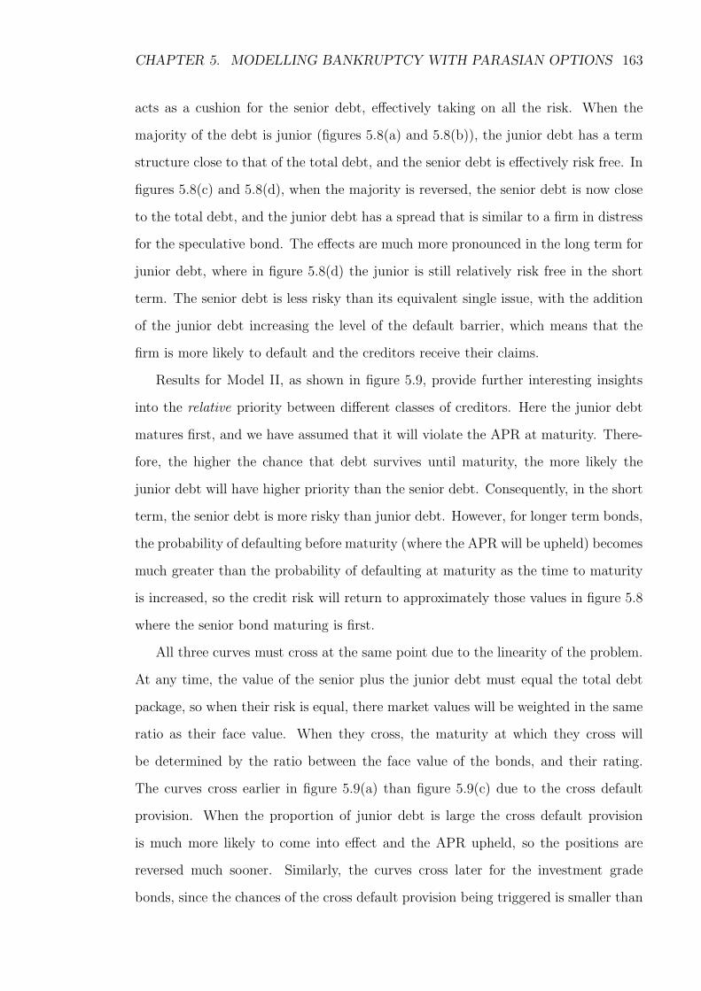
CHAPTER 5. MODELLING BANKRUPTCY WITH PARASIAN OPTIONS 163
acts as a cushion for the senior debt, effectively taking on all the risk. When the
majority of the debt is junior (figures 5.8(a) and 5.8(b)), the junior debt has a term
structure close to that of the total debt, and the senior debt is effectively risk free. In
figures 5.8(c) and 5.8(d), when the majority is reversed, the senior debt is now close
to the total debt, and the junior debt has a spread that is similar to a firm in distress
for the speculative bond. The effects are much more pronounced in the long term for
junior debt, where in figure 5.8(d) the junior is still relatively risk free in the short
term. The senior debt is less risky than its equivalent single issue, with the addition
of the junior debt increasing the level of the default barrier, which means that the
firm is more likely to default and the creditors receive their claims.
Results for Model II, as shown in figure 5.9, provide further interesting insights
into the relative priority between different classes of creditors. Here the junior debt
matures first, and we have assumed that it will violate the APR at maturity. There-
fore, the higher the chance that debt survives until maturity, the more likely the
junior debt will have higher priority than the senior debt. Consequently, in the short
term, the senior debt is more risky than junior debt. However, for longer term bonds,
the probability of defaulting before maturity (where the APR will be upheld) becomes
much greater than the probability of defaulting at maturity as the time to maturity
is increased, so the credit risk will return to approximately those values in figure 5.8
where the senior bond maturing is first.
All three curves must cross at the same point due to the linearity of the problem.
At any time, the value of the senior plus the junior debt must equal the total debt
package, so when their risk is equal, there market values will be weighted in the same
ratio as their face value. When they cross, the maturity at which they cross will
be determined by the ratio between the face value of the bonds, and their rating.
The curves cross earlier in figure 5.9(a) than figure 5.9(c) due to the cross default
provision. When the proportion of junior debt is large the cross default provision
is much more likely to come into effect and the APR upheld, so the positions are
reversed much sooner. Similarly, the curves cross later for the investment grade
bonds, since the chances of the cross default provision being triggered is smaller than
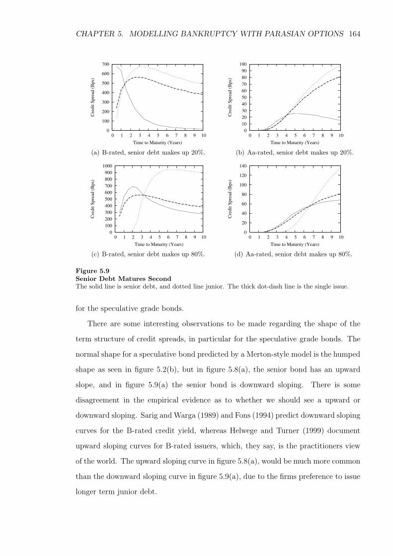
CHAPTER 5. MODELLING BANKRUPTCY WITH PARASIAN OPTIONS 164
0
100
200
300
400
500
600
700
0 1 2 3 4 5 6 7 8 9 10
Cre
dit
Sp
read
(B
ps)
Time to Maturity (Years)
(a) B-rated, senior debt makes up 20%.
0
10
20
30
40
50
60
70
80
90
100
0 1 2 3 4 5 6 7 8 9 10
Cre
dit
Sp
read
(B
ps)
Time to Maturity (Years)
(b) Aa-rated, senior debt makes up 20%.
0
100
200
300
400
500
600
700
800
900
1000
0 1 2 3 4 5 6 7 8 9 10
Cre
dit
Sp
read
(B
ps)
Time to Maturity (Years)
(c) B-rated, senior debt makes up 80%.
0
20
40
60
80
100
120
140
0 1 2 3 4 5 6 7 8 9 10
Cre
dit
Sp
read
(B
ps)
Time to Maturity (Years)
(d) Aa-rated, senior debt makes up 80%.
Figure 5.9Senior Debt Matures SecondThe solid line is senior debt, and dotted line junior. The thick dot-dash line is the single issue.
for the speculative grade bonds.
There are some interesting observations to be made regarding the shape of the
term structure of credit spreads, in particular for the speculative grade bonds. The
normal shape for a speculative bond predicted by a Merton-style model is the humped
shape as seen in figure 5.2(b), but in figure 5.8(a), the senior bond has an upward
slope, and in figure 5.9(a) the senior bond is downward sloping. There is some
disagreement in the empirical evidence as to whether we should see a upward or
downward sloping. Sarig and Warga (1989) and Fons (1994) predict downward sloping
curves for the B-rated credit yield, whereas Helwege and Turner (1999) document
upward sloping curves for B-rated issuers, which, they say, is the practitioners view
of the world. The upward sloping curve in figure 5.8(a), would be much more common
than the downward sloping curve in figure 5.9(a), due to the firms preference to issue
longer term junior debt.

CHAPTER 5. MODELLING BANKRUPTCY WITH PARASIAN OPTIONS 165
200
400
600
800
1000
1200
0 0.05 0.1 0.15
Volatility σr
Cre
dit
Spre
ad
(bps)
(a) B = 20
0
200
400
600
800
0 0.05 0.1 0.15
Volatility σr
Cre
dit
Spre
ad
(bps)
(b) B = 80
Figure 5.10Credit Spread vs. Volatility of Interest RateCredit spreads for the senior, junior and total debt are shown from top to bottom. The correlation
parameter ρ is varied from −0.5 (solid), 0 (dashed) and 0.5 (dotted) for each of the three bonds. (a)
Top to bottom are the junior, total and senior debt curves with senior debt making up 20% of the
total debt. (b) Top to bottom are the junior, total and senior debt curves with senior debt making
up 80% of the total debt.
The shape of the credit spread curve appears to be affected not only by the
seniority structure, but also the relative weight and maturity structure. For the
speculative bond when the junior has a shorter maturity, the senior bond changes
from a downward slope in figure 5.9(a) to a humped shape in figure 5.9(c). Then, for
the junior bond, in figure 5.9(c) the weighting between the two bonds results in an
unusual curve, which is very safe at the short end, then very risky at the long end,
while in figure 5.9(a) the junior displays the normal humped shape.
5.6.2 Credit spread and interest rate volatility
In our model we take interest rate parameters from Huang and Huang (2003), and
in figure 5.10 we demonstrate the effect of some of those parameters. The model is
sensitive to the volatility of interest rates, but equally so to the correlation between
the interest rate and the firm value. When the correlation is negative, an increase in
interest rate volatility can actually result in the credit spread decreasing (see Acharya
and Carpenter, 2002). The effect of the of the correlation is large even for the modest
range of interest rate volatility (0-15%) shown.

CHAPTER 5. MODELLING BANKRUPTCY WITH PARASIAN OPTIONS 166
0
100
200
300
400
500
600
-20020406080
Cre
dit
Sp
read
(B
ps)
Distance between default barrier and senior debt level
(a) B-rated, senior debt makes up 20%.
0
20
40
60
80
100
120
-20020406080
Cre
dit
Sp
read
(B
ps)
Distance between default barrier and senior debt level
(b) Aa-rated, senior debt makes up 20%.
0
100
200
300
400
500
600
700
800
900
1000
-80-60-40-20020
Cre
dit
Sp
read
(B
ps)
Distance between default barrier and senior debt level
(c) B-rated, senior debt makes up 80%.
0
50
100
150
200
250
-80-60-40-20020
Cre
dit
Sp
read
(B
ps)
Distance between default barrier and senior debt level
(d) Aa-rated, senior debt makes up 80%.
Figure 5.11Credit Spread vs. Default Barrier Level, with Senior Debt Maturing FirstThe solid line is senior debt, and dotted line junior. The thick dot-dash line is the single issue.
5.6.3 Credit spread and default barrier
So far, all results have taken the barrier to be at level of total debt, which Yu
(2004) assumes is the situation where the junior creditors fully cooperate with the
senior creditors. Here in this section we investigate an internal bargaining between
the creditors, resulting in a change in the level of the default barrier. Figure 5.11
shows the credit spread of the senior, junior and total debt at a maturity of ten years
against the position of the default barrier. The position is given as its distance from
the senior debt level, with positive indicating above and negative below. The total
debt shows the result of the internal bargain on the debtors.
We know that when the barrier is lowered, the chance that the ParAsian option
will be knocked out is reduced, so we expect credit spread to increase. Conversely,
as the barrier level is increased, the higher the chance that the ParAsian option is

CHAPTER 5. MODELLING BANKRUPTCY WITH PARASIAN OPTIONS 167
knocked out and the creditors receive their full claim, so the credit spread should de-
crease. Consequently we would expect credit spread to be a monotonically decreasing
function of the barrier level, however, figure 5.11 shows this is not always the case.
First, we note that as the barrier level approaches zero, the curves plateau. When
the barrier is so small, the likelihood of the ParAsian option being knocked out is
so small that the option becomes effectively European. The curves displayed by
the senior bond are quite easy to explain, given that all curves are monotonically
decreasing, with the senior debt curves in figures 5.11(c) and 5.11(d) almost identical
to the total debt. Although the senior curves in figures 5.11(a) and 5.11(b) appear to
be quite different to the total debt curves, if we were to plot the total debt curves and
let the barrier extend out to four or five times the total debt level, we should expect
that the curves will look the same. The reason that the decrease in credit spread
is so steep around the senior debt level is due to the discontinuity in the boundary
condition at the senior debt level. Above this level, the creditors will receive their
full claim rather than a portion of it when below the level.
More interesting however, are those results observed for the junior debt. The
credit spread is no longer a monotonically decreasing function of the barrier, actually
increasing over some range of barrier values, for instance in figure 5.11(a) the credit
spread increases between [−20, 40]. As the barrier value is increases from zero above
the senior value the probability of default gradually increases, but since the junior
creditors are likely to end up with nothing if the bond defaults, they are actually worse
off. The result is that the curve is initially increasing, before this effect is offset by the
increasing recovery value that the junior creditors will receive at default, until they
are close to (possibly) receiving their full claim and the curve starts to decrease. The
barrier level at which the spread will stop increasing is obviously highly dependent
on the weighting of junior to senior. In figures 5.11(a) and 5.11(b) where the senior
debt level is low, the junior creditors start to receive a benefit from default much
faster than in figures 5.11(c) and 5.11(d) where the senior holds the larger proportion
of debt.
When the junior debt matures first, the position of the barrier can play an even

CHAPTER 5. MODELLING BANKRUPTCY WITH PARASIAN OPTIONS 168
0
100
200
300
400
500
600
-20020406080
Cre
dit
Sp
read
(B
ps)
Distance between default barrier and senior debt level
(a) B-rated, senior debt makes up 20%.
0
20
40
60
80
100
120
-20020406080
Cre
dit
Sp
read
(B
ps)
Distance between default barrier and senior debt level
(b) Aa-rated, senior debt makes up 20%.
0
100
200
300
400
500
600
700
800
900
-80-60-40-20020
Cre
dit
Sp
read
(B
ps)
Distance between default barrier and senior debt level
(c) B-rated, senior debt makes up 80%.
0
20
40
60
80
100
120
140
-80-60-40-20020
Cre
dit
Sp
read
(B
ps)
Distance between default barrier and senior debt level
(d) Aa-rated, senior debt makes up 80%.
Figure 5.12Credit Spread vs. Default Barrier Level, with Senior Debt Maturing SecondThe solid line is senior debt, and dotted line junior. The thick dot-dash line is the single issue.

CHAPTER 5. MODELLING BANKRUPTCY WITH PARASIAN OPTIONS 169
more important role than in the previous case. While figures 5.12(a) and 5.12(b)
show similar trends to those observed in figure 5.11, figures 5.12(c) and 5.12(d) show
quite different results. By changing the level of the barrier, the junior can become
senior, and vi ca versa. This is due to the fact that even at a maturity of ten years,
the European option values for the junior and senior bonds are switched, with the
senior having a higher credit spread than the junior. Since the ParAsian knockout
will have the same effect as before, i.e. that the senior is decreasing and the junior is
initially increasing, their positions are eventually returned to normal. This effect is
lessened when the junior debt has a high proportion, since the cross-default provision
will influence the value of the European.
5.6.4 Credit spread and window length
We have already discussed the effect of the window on a single debt issue in
section 5.5.2, and here we compare the single issue results to those of senior and
junior bonds. As in the previous section where the default barrier influenced the
probability of the ParAsian option being knocked out, so it is with the window length.
The shorter the window length, the more likely the ParAsian will be knocked out,
and the longer it is the less likely it will be knocked out. This means that figures 5.13
and 5.14 follow very similar trends to those in figures 5.11 and 5.12. In fact, the
trends for the window length figures in the region T ∈ [2, 10], are identical to the
barrier figures, as this is the region where the option becomes more European.
In the limit as window length tends to zero, credit spreads across all bonds plunge
to zero. As mentioned earlier in section 5.5.2, because the barrier is placed at the total
debt level, the instant knocked out at the barrier with zero window length means that
all creditors receive their full claim. Conversely, as the window length tends to the
maturity length the probability of knockout approaches zero and the option becomes
European. We note again that in figures 5.14(c) and 5.14(d) the senior debt is more
risky than the junior debt when the ParAsian option becomes European.
When analysing the effect of window length for senior bond, the effect is similar

CHAPTER 5. MODELLING BANKRUPTCY WITH PARASIAN OPTIONS 170
0
100
200
300
400
500
600
0 2 4 6 8 10
Cre
dit
Sp
read
(B
ps)
Window Length (Years)
(a) B-rated, senior debt makes up 20%.
0
20
40
60
80
100
120
0 2 4 6 8 10
Cre
dit
Sp
read
(B
ps)
Window Length (Years)
(b) Aa-rated, senior debt makes up 20%.
0
200
400
600
800
1000
1200
0 2 4 6 8 10
Cre
dit
Sp
read
(B
ps)
Window Length (Years)
(c) B-rated, senior debt makes up 80%.
0
50
100
150
200
250
0 2 4 6 8 10
Cre
dit
Sp
read
(B
ps)
Window Length (Years)
(d) Aa-rated, senior debt makes up 80%.
Figure 5.13Credit Spread vs. Window Length, with Senior Debt Maturing FirstThe solid line is senior debt, and dotted line junior. The thick dot-dash line is the single issue.
CHAPTER 5. MODELLING BANKRUPTCY WITH PARASIAN OPTIONS 171
0
100
200
300
400
500
600
0 2 4 6 8 10
Cre
dit
Sp
read
(B
ps)
Window Length (Years)
(a) B-rated, senior debt makes up 20%.
0
20
40
60
80
100
120
0 2 4 6 8 10
Cre
dit
Sp
read
(B
ps)
Window Length (Years)
(b) Aa-rated, senior debt makes up 20%.
0
200
400
600
800
1000
1200
0 2 4 6 8 10
Cre
dit
Sp
read
(B
ps)
Window Length (Years)
(c) B-rated, senior debt makes up 80%.
0
20
40
60
80
100
120
140
160
180
200
0 2 4 6 8 10
Cre
dit
Sp
read
(B
ps)
Window Length (Years)
(d) Aa-rated, senior debt makes up 80%.
Figure 5.14Credit Spread vs. Window Length, with Senior Debt Maturing SecondThe solid line is senior debt, and dotted line junior. The thick dot-dash line is the single issue.

CHAPTER 5. MODELLING BANKRUPTCY WITH PARASIAN OPTIONS 172
to that felt by the total debt, especially when the proportion of senior debt is high.
In figures 5.13(a) and 5.13(b) the effect is step-like, with a window length of two or
less years not having much effect, and likewise six or more. In between the credit
spread rises (relatively) sharply, and the window length we have chosen is just outside
of this region, so for the senior debt a decrease in window length will have a small
effect as compared to an increase in window length.
For the junior debt, the trends are most interesting when the proportion of junior
debt is small. Again as the window length is reduced from the European value at
T = 10 (the chance of knockout increases), the credit spread is initially at least
increasing. Then around the one year mark, the credit spread drops dramatically
toward zero as not only the probability of knockout increases, but also the recovery
rate. The recovery rate increases as the window length decreases as the average
distance the process can travel below the barrier is decreased as the window length
is decreased.
5.7 Conclusions
In this chapter we systematically model corporate debt, both for a single class of
debt and for two debt classes, under a variety of seniority and maturity structures,
testing several variants of ParAsian option to model the process prior to possible
bankruptcy. Results for the single debt class show the practicality of the ParAsian
window which, amongst other effects, increases credit spreads. Different structures
present some unique characteristics of corporate bonds in a two-class debt structure.
These characteristics include the shapes and magnitudes of the term structures of
credit spreads, the sensitivities of credit spreads to the volatility of asset, the initial
interest-rate level and the volatility of interest rate, as well as bond durations. The
results for the senior debt are consistent with an otherwise identical debt but improved
credit status. However, the results for the junior debt can be counterintuitive, owing
to its equity trait, the degree of which is governed by its weight in the total debt and
the maturity structure.

CHAPTER 5. MODELLING BANKRUPTCY WITH PARASIAN OPTIONS 173
Importantly, a propos each model, we further investigate the bargaining power
of the junior creditors and debtors, as well as the interaction between these two, by
means of changing the default barrier and the ParAsian window. We find that both
make the senior creditors worse off, though to different extents according to their
proportions in the total debt as well as the firm’s credit status. The story is more
complicated in the junior case, in that the junior debt has mixed features of debt and
equity. The junior creditors mainly exert their bargaining power when they are more
susceptible to credit deterioration or they are able to seize the chronological priority
at maturity. They can also benefit from a stronger bargaining power of the debtors,
where it is possible that interests become aligned.

Chapter 6
Convertible Bonds
The unique manner in which convertible bonds combine features of both equity
and debt has made them an attractive solution to firms wishing to raise capital and,
unsurprisingly, a popular investment tool. They are also notoriously difficult to price
relative to the underlying stock, with any number of factors from market illiquidity
to market psychology giving arbitrage opportunities for fund managers to exploit.
As the name suggests, the convertible bond gives the owner the option to exchange
the bond for some prearranged number of stocks in the issuing firm. The conversion
policy is usually expressed as either the conversion ratio (the ratio of stocks to bonds
that can be exchanged) or the conversion price (the stock price above which the holder
may exchange at maturity). The convertible bond is a hybrid security, a combination
of both debt and equity. The bond component will provide the holder with interest
payments, though these are usually lower than a normal corporate bond, which is
offset by the potential gains if the stock price rises and the holder wishes to convert.
The bond appears to offer a win-win situation, unless of course the bond defaults in
which case the holder will incur losses.
The holder may convert at any time during the contract, making this an American-
style contract. There are also two other American options often in the contract; one,
the call, will limit the upside potential, and the other, the put, will limit the downside
potential. The call gives the issuer the option to make the holder choose, over a short
period of time, either to convert the bond or to exchange it for a cash sum equal to
174

CHAPTER 6. CONVERTIBLE BONDS 175
the call price. This is usually a function of time, and defined for all future times in
the contract. To encourage the purchase of these bonds, there is often a hard call
protection period during which the firm is prohibited from calling the bond back.
During the soft call protection period, the company can call the bond back, but
only if the stock price is above some trigger price for more than 30 days. The put
option on a premium put convertible means that the holder may sell back the bond
to the issuer at a premium at any time before maturity, during certain periods or
on specified dates. Grimwood and Hodges (2002) find that almost all bonds in their
sample have an embedded call option, with a significant proportion also having some
form of put option also.
We aim to extend the current convertible bond literature in two ways. First, to
model the default of the bond, we will adopt the Yu (2004) framework as discussed
in chapter 5. Second, we will attempt to price the convertible bond issue in a more
complex capital structure framework than is usually attempted. We will see the effect
of senior bond issues on the price of the convertible, as well as its effect on the optimal
call and conversion policies.
6.1 Literature
There have been two main approaches to the problem of valuing convertible bonds,
both of which are structural, but depend on whether the stochastic process is the
value of the firm (firm models), or the value of the stock (equity models). There are
obvious advantages and disadvantages to both, such as the fact that the firm value
cannot be observed, but can model default in a better way, whilst equity models can
take data straight from the market, but cannot model default very well.
Ingersoll (1977b) was the first to propose a model for convertible bonds which
are modelled as a contingent claim on the firm value. This is a primitive model,
though, and assumptions that are now commonly relaxed (default only at maturity,
no dividend payments, constant interest rates) are enforced here. These assumptions
guarantee that the problem has a closed form solution, which is presented in Ingersoll
CHAPTER 6. CONVERTIBLE BONDS 176
(1977b).
Relaxing the assumptions made by Ingersoll (1977b) leads to the problem no
longer having a closed form solution. For this reason, Brennan and Schwartz (1977a)
propose an implicit numerical scheme to price the convertible bond, which permits
the model to include dividend/coupon payments, American style conversion, optimal
calling of the bond and the possibility of default before maturity. They later extend
the model to include stochastic interest rates (Brennan and Schwartz, 1980) in a two-
factor model. One of the main results from the paper is that stochastic interest rates
have little effect on the solution, although the argument for abandoning them seems
to be for the ease of solution rather than effective pricing. Brennan and Schwartz
(1980) also outline how one would go about solving for a convertible bond with a
more complicated capital structure, i.e. the firm is made up of a senior issue, the
convertible and equity. The results in this paper do not pay attention to the effect of
the senior issue on the price of the convertible.
Nyborg (1996) defines how the Brennan and Schwartz (1980) model may in-
corporate a put option, without actually solving the PDE presented in the paper.
Carayannopoulos (1996) tests the Brennan and Schwartz model using the CIR inter-
est rate model (Cox et al., 1985) rather than the Vasicek (1977) style rates used by
Brennan and Schwartz. They find that in some circumstances the stochastic interest
rate can have a large effect on the accuracy of the pricing model. The barrier at
which default occurs is particularly low, bonds only default if the firm value is less
than the next coupon payment, which is unrealistic – firms normally default much
sooner than this.
McConnell and Schwartz (1986) were the first to deviate from the firm value
analysis for convertible bonds, choosing instead to model the option using the firm’s
stock as the underlying process. The Liquid Yield Option Note (LYON) that they
price, is callable, puttable, and convertible, making it rather a complicated problem,
and so equity is chosen as the underlying to reduce the complexity of the problem.
If the firm has other debt that it is senior to the issued debt, under the firm value
analysis this must be valued first in order to value the convertible debt. McConnell

CHAPTER 6. CONVERTIBLE BONDS 177
and Schwartz realise they cannot model default with equity as the underlying process,
so simply ‘gross’ up the risk-free interest rate to capture default risk, to compensate
for the underpricing of the model. The model they present is easily solved using
simple finite-difference methods, and can be extended to include stochastic interest
rates. The simplification of the model however, is not always appropriate, since the
credit risk is (intuitively) not constant across all share prices.
The first interpretation that the convertible bond with its hybrid nature should
have different discount rates for its equity and debt parts is by Goldman Sachs (1994).
Using the first derivative ∂V∂S
(the delta hedge) value as an indication of the probability
that the debt was to be converted into equity, they form a discount rate in which the
risky part is related to this probability of conversion. This achieves something in that
the bond is more risky at low share prices, and less so as the share price increases,
but it has little financial or economic backing for such a weighting.
Ho and Pfeffer (1996) also propose an idea that the bond should be split into
components, some of which are subject to credit risk, and some that are not. The
convertible bond is split into the sum of a straight bond (subject to credit risk), a
warrant (not subject to credit risk) and a forced conversion option. The bond is split
using the argument that the warrant will not be exercised before maturity, so the
option is not American as such. American options cannot be split so easily, since
they have non-linear boundary conditions, and as a consequence this model will not
work if it is optimal for the convertible bond-holders to exercise before maturity,
although the model does incorporate the yield curve into the solution, using the Ho
and Lee (1986) model of interest rates.
A popular equity model developed by Tsiveriotis and Fernandes (1998) also splits
the bond into two parts; however the convertible bond is not the sum of the two parts,
but both parts are linked via coupled PDEs. They consider that the ‘cash-only’ part of
the bond should be subject to default risk while the remaining part of the convertible
bond is not. The cash-only component is priced as a digital option with a knock-
out barrier where the convertible bond is converted. The convertible bond is then
priced in the usual fashion, with the discount rate adjusted according to the value
CHAPTER 6. CONVERTIBLE BONDS 178
of the cash-only component. The fact that the rate at which the convertible bond
is discounted is linked to the conversion strategy of the holder, through boundary
conditions for the cash-only part, seems to contradict the notion that the default
of the firm, and hence the credit risk, is independent of the strategy taken by the
convertible bondholders. Furthermore, the firm does not default (at least no loss is
incurred) even if the stock price reaches zero. There are, therefore, some obvious
flaws in this model.
A more recent approach, developed by Davis and Lischka (1999), Takahashi et al.
(2001) and Ayache et al. (2003) is to follow a reduced form approach to default
(Jarrow and Turnbull, 1995; Duffie and Singleton, 1999; Madan and Unal, 2000). In
contrast with the structural approach, default is now an exogenous process, which
can happen instantaneously at any time. The probability of default is captured in the
hazard rate (a function of the stock price that may itself be stochastic) and at default
the bond holder is assumed to receive some compensation. The model by Ayache
et al. (2003) is the only study which discusses what happens at default, whereas
other studies assume either total or zero recovery. The model is also driven by the
fundamental principles of the continuous hedge and no-arbitrage, which are somewhat
circumvented by Tsiveriotis and Fernandes (1998) with their ad hoc splitting of the
bond, which Ayache et al. (2003) show to be inconsistent. However, all of the equity
models discussed here have problems attributed to the exogenous nature of default,
such as predicting unrealistic prices (a risky bond may be worth more than a riskless
one); no possibility of a reorganisation period or emergence from bankruptcy; the
dilution of the firm share price is not taken into account.
Bermudez and Webber (2004) attempt a cross-over model, part structural, part
reduced form in order to endogenise both default and the recovery rate. The recovery
rate is endogenised in the sense that there is a reorganisation period during which
the creditors must wait to receive compensation, in which time the value of the firm
(that they will receive) is allowed to move stochastically. So, in short, they surrender
a European put which is exercised at the end of the reorganisation period. This
is different from a Parisian or ParAsian option, since the firm cannot emerge from
CHAPTER 6. CONVERTIBLE BONDS 179
the reorganisation under the Bermudez and Webber (2004) framework. This greatly
simplifies the pricing of the option, which they simplify further by using the Vasicek
(1977) interest model, allowing them to value the European put with an explicit
formula when the correlation (between asset and interest rate) is zero; in fact they
also use the formula even when the correlation is not zero. The firm may default
either when payments by the firm cannot be made (endogenous) or at some jump
time of a counting process (exogenous), where the firm value is reduced by some
proportion of its current value. The probability of the firm defaulting endogenously
is slim, however, and exogenous default will still account for the majority of the
default risk. The firm only appears to pay coupons, not dividends, which greatly
simplifies the computation, since the problem is not American unless dividends are
present.
In the next section we develop a model using the Yu (2004) framework under
which the default risk of the bond is correctly valued against the equity conversion.
The model allows for all possible embedded options to be present, with a simple
modification of boundary conditions. The model can also show how the capital
structure of the firm can have a large effect on the price, something overlooked in
the majority of the literature (which effectively takes the senior priority debt to
be risk-free); convertible bonds are often issued by firms with outstanding debt as
subordinate bonds. This also introduces an interesting problem in that the price of
the senior debt may also be affected by the issue of convertible debt. If the convertible
debt matures first (c.f. section 5.2), then the convertible debt holders may be able
to violate the APR reducing the senior debt holders claim on the firm. Conversely,
the convertible debt provides a cushion to the senior debt that increases its recovery
rate, which may be removed if the convertible debt holders convert to shares. There
is clearly a complex interplay between the creditors.

CHAPTER 6. CONVERTIBLE BONDS 180
6.2 The Model
First we define the convertible bond following the framework of Brennan and
Schwartz (1980). We assume that the firm is made up of senior debt holders, the
convertible bond issue and the shareholders. Then we may express value of the firm
to be
V = Nb B +Nc C +Ns S. (6.1)
where Nb, Nc, and Ns are the number of senior bonds, convertible bonds and shares
respectively. B is the value of a single senior bond, C the value of a convertible bond,
and S the value of a share.
Let us examine what happens to the value of the firm at conversion. Now note
that before conversion we have
V BC = Nb B +Nc C +Ns SBC ,
and after conversion
V AC = Nb B + (∆N +Ns) SAC ,
where ∆N = q.Nc. Then the fraction of shares owned by the holder of each of the
convertible bonds is
Z = q/(∆N +Ns),
the so called dilution factor.
Next, the conversion value for each of the bonds can be expressed in two ways,
using either the share price before conversion or the share price after conversion. We
then have
Conversion Value(1) = q.SBC (6.2)
Conversion Value(2) = q.SAC , (6.3)
and so when equating with previous equations we arrive at two different prices for
CHAPTER 6. CONVERTIBLE BONDS 181
the convertible bond at conversion,
Conversion Value(1) =q
Ns
.[V −Nb B −Nc C] (6.4)
Conversion Value(2) = Z.[V −Nb B]. (6.5)
If we assume that SBC = SAC and equate equations (6.2) and (6.3) then
q
Ns.[V −Nb B −Nc C] =
q
∆N +Ns.[V −Nb B],
will become
(∆N +Ns).[V −Nb B −Nc C] = Ns.[V −Nb B]
(∆N +Ns).Nc C = ∆N.[V −Nb B]
C = Z.[V −Nb B]. (6.6)
Consequently, only if the convertible bond is selling at the conversion price will the
two equations be consistent.
6.2.1 The Governing PDE
We aim to price the convertible bond as a contingent claim on the value of the
firm. We assume that the value of the firm moves under a geometric Brownian motion
dV
V= µ dt+ σv dZV . (6.7)
The instantaneous interest rate, r, is assumed to follow the Cox et al. (1985) model,
dr = κ(θ − r)dt+ σr
√rdZr, (6.8)
where r is a mean-reverting process. The two processes are correlated via the param-
eter ρ,
dZV dZr = ρ dt. (6.9)
CHAPTER 6. CONVERTIBLE BONDS 182
Following the analysis in chapters 4 and 5 we model the default of the firm via a
ParAsian option. Then defining the time under reorganisation as the barrier time t,
which is characterised by equation 4.17, we arrive at the following PDE to describe
the price of the convertible bond:
Ct + Ct +1
2CV V σ
2V V
2 +1
2Crrσ
2rr + CV rσV V σr
√rρ
+Cr
(
κ(θ − r)− λσr
√r)
+ rCV = rC if V ≤ K (6.10)
Ct +1
2CV V σ
2V V
2 +1
2Crrσ
2rr + CV rσV V σr
√rρ
+Cr
(
κ(θ − r)− λσr
√r)
+ rCV = rC if V > K, (6.11)
where K is the default barrier described later.
6.2.2 At Maturity
We assume, as we did previously in chapter 5, that both the senior and convert-
ible bond issues mature at the same time (although it is possible to allow for the
convertible issue to mature slightly earlier, which may result in a violation of the
APR). Let us assume intially that the APR is upheld, then at maturity each senior
bond holder will receive the face value of the bond (and the final coupon payment for
a coupon bond) unless the firm cannot afford to pay back all the senior bondholders,
and so at maturity they receive
B(V, r, T, t ) =
1NbV if V < Nb Fb
Fb if V ≥ Nb Fb
. (6.12)
If the value of the firm is high, then the convertible bondholders may choose to
convert. However, if it is low, the convertible bondholders have a claim on the firm
CHAPTER 6. CONVERTIBLE BONDS 183
so long as the senior bondholders have already been fully paid.
C(V, r, T, t ) =
0 if V < Nb Fb
1Nc
[V −Nb Fb] if 0 ≤ 1Nc
[V −Nb Fb] < Fc
Fc if Z · [V −Nb Fb] < Fc ≤ 1Nc
[V −Nb Fb]
Z · [V −Nb Fb]. if Z · [V −Nb Fb] ≥ Fc .
(6.13)
6.2.3 Default Barrier
For simplicity, we assume that the firm will not issue any new debt to keep to
a target leverage ratio (as in Collin-Dufresne and Goldstein, 2001). Then defining
L(r, t;T, cl) to be the value of an otherwise equivalent risk-free coupon paying bond,
Fb and Fcb as the face value of a senior and convertible bond respectively, and cb and
ccb their respectivecoupon payments, then we choose cl such that
cl =Nb Fb
Nb Fb +Nc Fcb
cb +Nc Fcb
Nb Fb +Nc Fcb
ccb ,
which is equivalent to the total coupon paid out by the firm. Then the barrier, K
(c.f. section 5.3), is placed at the value of an equivalent riskfree debt to that of the
total debt in the firm;
K(r, t) = (Fb + Fcb) L(r, t;T, cl). (6.14)
The barrier need not necessarily be placed at the total debt level if bargaining similar
to that described in chapter 5 takes place, but it could be placed somewhere between
the senior debt level and the total debt level. If the firm cannot undergo a period of
reorganisation and instantly defaults, placing the barrier at or above the senior debt
levels makes the senior debt riskfree, which is the assumption most models make.
Here, as in the previous chapter we allow a reorganisation period of two years, for
reasons defined in chapter 5, so that the senior debt is not risk-free and will influence
the price of the convertible debt depending on the ratio between the two of them.

CHAPTER 6. CONVERTIBLE BONDS 184
6.2.4 Optimal Call and Conversion
If the convertible bondholders act optimally, they will choose to exercise only when
the return on dividend payments exceeds the proposed coupon payment. Although,
under this framework, we allow the dividend payment to be continuous, in reality the
dividend payment will be discontinuous, implying that the convertible bondholders
will only convert just before a dividend payment: the option is effectively Bermudan.
However, by allowing continuous payments we gain more insight into the dynamics
of the problem. At conversion, the bondholders receive Z [V − Nb B], so the value
of the option must be always greater than this value;
C(V, r, t, t) ≥ Z (V −Nb B). (6.15)
We assume that the firm may call back the convertible bond at a predetermined
call price. Now under the Brennan and Schwartz (1980) framework, the share price
is also viewed as a contingent claim on the firm value. When the firm contains only
non-convertible debt, the shareholders hold a (perpetual) call option on the firm’s
assets with strike price at the face value of debt. If the firm issues convertible debt,
the share holders effectively write an (American) call option (on the firm value) to
the convertible bond holders, which could (if converted) result in their stake in the
firm being reduced1. The share price process follows the same PDE as that governing
the convertible bond, with appropriate boundary conditions. Of interest here is that
under the firm value model, the movement of the share price reacts to the impending
conversion. The process that the share price undergoes is different, depending on
whether the convertible debt is acting like debt or equity, in this way the process for
the share price is nonlinear, it is the process of the total firm that stays log-normal.
In equity models, the share price is assumed to follow the same process, regardless of
whether the convertible bonds are acting like debt or equity, but impending conversion
has been shown to affect the share price.
If the firm is acting optimally, then the management will choose to maximise the
1Some convertible bond issue have covenants protecting the shareholder from dilution.
CHAPTER 6. CONVERTIBLE BONDS 185
value of the shares, which, from (6.1) means they must minimise the value of the
convertible bonds. Therefore, they will exercise the right to call back the bonds the
first instant that the value of the bonds exceed the call price, hence
C(V, r, t, t) ≤ Cp. (6.16)
There is empirical evidence to suggest that firms do not always act optimally
and call the bonds back after they have exceeded the call price by on average 43%
(Ingersoll, 1977a). A framework for modelling the delay in exercising an option, is
explored later, in chapter 7. If the call has the soft-call constraint (where the share
price must be above some barrier for a predetermined amount of time, modelled by
Avellaneda et al., 1999 as a Parisian option) this will present a problem since, as
mentioned above, the value of the shares is a function of the firm value and not of
the underlying asset, and therefore cannot be modelled as a simple Parisian type
option. The delayed exercise framework in chapter 7 makes it possible to value such
an option in the firm value model.
6.3 Numerical methods
The technique used to solve this problem must be quick and efficient to solve
what is essentially a four dimensional free boundary problem. We choose to adapt
the boundary-updating solver from chapter 3. The method is flexible and is around
ten-times faster than the equivalent PSOR method. In order to adopt this method,
we must abandon the Crank-Nicolson scheme in favour of an implicit scheme. The
Crank-Nicolson scheme is prone to ringing in ParAsian/Parisian options due to dis-
continuities in option price at zero barrier time, which are fully explained in chapter 4.
Any such errors in the scheme (such as negative option prices for small V ) may be
amplified through from the senior bond solution to the convertible bond, possibly
causing the boundary-updating solver not to work. We do not choose an explicit
scheme since time step restrictions for the ParAsian option result in a hefty increase

CHAPTER 6. CONVERTIBLE BONDS 186
Table 6.1Convergence of the convertible bond price
n m p C(V0, r0, 0, 0) CRE CRE2
41 5 9 1012.981 9 17 1009.3 1005.7161 17 33 1009.2 1009.0 1010.1321 33 65 1009.2 1009.3 1009.4641 65 129 1009.3 1009.4 1009.41281 129 257 1009.3 1009.4 1009.4
A table showing the convergence of the implicit method used in this chapter. We price a B-rated
bond convertible bond in a two-tier debt structure with parameters as defined in table 6.2, at the
given firm value V0 and interest rate r0. n, m and p are the number of points in V , r and t
respectively. The grid is contained by V ∈ [0 : 8Ft], r ∈ [0 : 4r0] and t ∈ [0, 2] The value of the
straight calculation is shown in the fourth column, with once and then twice extrapolated results
(Richardson extrapolation, see chapter 4) in the fifth and sixth columns respectively.
in calculations since we require ∆t = ∆t, therefore halving the time steps increases
computation time four-fold.
In table 6.1 we show the convergence of the convertible bond price. The implicit
scheme adopted here is not as effective as the Crank-Nicolson scheme adopted in
previous chapters, and the convergence is not quite as smooth as that seen by the
straight bond (see section 5.4, table 5.2), which may be due to any one of a number
of factors, such as non-linearity from the free boundary, or contaminating errors from
the senior bond calculations. As a result of non-smooth convergence the Richardson
extrapolation is not as effective as seen previously. We must solve here over a larger
grid (V ∈ [0 : 8Ft]) than the straight bond (V ∈ [0 : 8Ft]) in order to take both the
debt and equity of the convertible bond into account. Therefore, the values of dV
are twice as large as those in the corresponding entries in table 5.2, so we should not
expect similar accuracy to those results. Note here that, if we set dV to be the same
as before, the greater grid size results in a calculation over so many nodes that even
a top range computer with 8Gbs of RAM could not handle the calculation. We do
however have a price for the bond that is accurate to the nearest 10¢ on bond with
a $1000 face value, which is adequate enough.
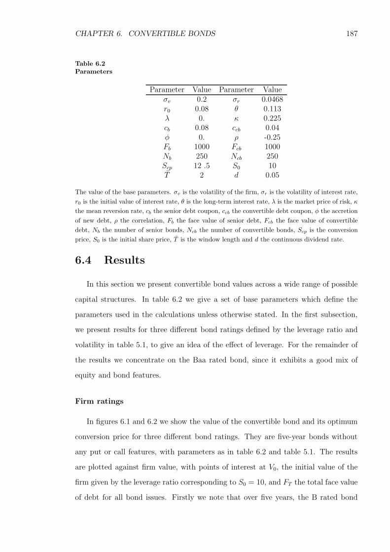
CHAPTER 6. CONVERTIBLE BONDS 187
Table 6.2Parameters
Parameter Value Parameter Valueσv 0.2 σr 0.0468r0 0.08 θ 0.113λ 0. κ 0.225cb 0.08 ccb 0.04φ 0. ρ -0.25Fb 1000 Fcb 1000Nb 250 Ncb 250Scp 12 .5 S0 10T 2 d 0.05
The value of the base parameters. σv is the volatility of the firm, σr is the volatility of interest rate,
r0 is the initial value of interest rate, θ is the long-term interest rate, λ is the market price of risk, κ
the mean reversion rate, cb the senior debt coupon, ccb the convertible debt coupon, φ the accretion
of new debt, ρ the correlation, Fb the face value of senior debt, Fcb the face value of convertible
debt, Nb the number of senior bonds, Ncb the number of convertible bonds, Scp is the conversion
price, S0 is the initial share price, T is the window length and d the continuous dividend rate.
6.4 Results
In this section we present convertible bond values across a wide range of possible
capital structures. In table 6.2 we give a set of base parameters which define the
parameters used in the calculations unless otherwise stated. In the first subsection,
we present results for three different bond ratings defined by the leverage ratio and
volatility in table 5.1, to give an idea of the effect of leverage. For the remainder of
the results we concentrate on the Baa rated bond, since it exhibits a good mix of
equity and bond features.
Firm ratings
In figures 6.1 and 6.2 we show the value of the convertible bond and its optimum
conversion price for three different bond ratings. They are five-year bonds without
any put or call features, with parameters as in table 6.2 and table 5.1. The results
are plotted against firm value, with points of interest at V0, the initial value of the
firm given by the leverage ratio corresponding to S0 = 10, and FT the total face value
of debt for all bond issues. Firstly we note that over five years, the B rated bond
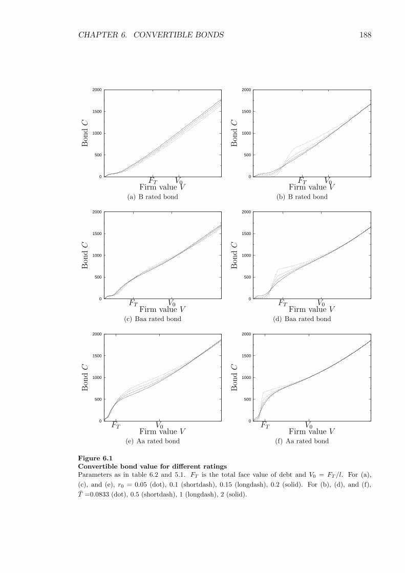
CHAPTER 6. CONVERTIBLE BONDS 188
0
500
1000
1500
2000
FT V0Firm value V
Bon
dC
(a) B rated bond
0
500
1000
1500
2000
FT V0Firm value V
Bon
dC
(b) B rated bond
0
500
1000
1500
2000
FT V0Firm value V
Bon
dC
(c) Baa rated bond
0
500
1000
1500
2000
FT V0Firm value V
Bon
dC
(d) Baa rated bond
0
500
1000
1500
2000
FT V0Firm value V
Bon
dC
(e) Aa rated bond
0
500
1000
1500
2000
FT V0Firm value V
Bon
dC
(f) Aa rated bond
Figure 6.1Convertible bond value for different ratingsParameters as in table 6.2 and 5.1. FT is the total face value of debt and V0 = FT /l. For (a),
(c), and (e), r0 = 0.05 (dot), 0.1 (shortdash), 0.15 (longdash), 0.2 (solid). For (b), (d), and (f),
T =0.0833 (dot), 0.5 (shortdash), 1 (longdash), 2 (solid).
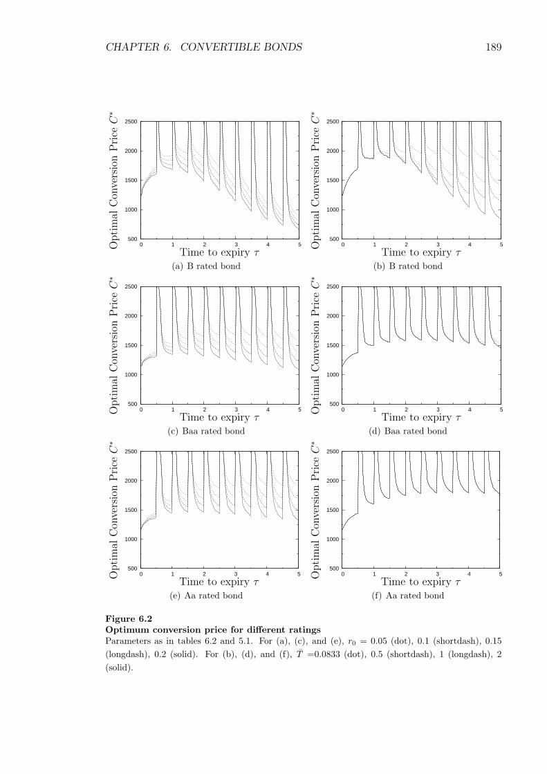
CHAPTER 6. CONVERTIBLE BONDS 189
500
1000
1500
2000
2500
0 1 2 3 4 5
Time to expiry τ
Opti
mal
Con
vers
ion
Pri
ceC
∗
(a) B rated bond
500
1000
1500
2000
2500
0 1 2 3 4 5
Time to expiry τ
Opti
mal
Con
vers
ion
Pri
ceC
∗
(b) B rated bond
500
1000
1500
2000
2500
0 1 2 3 4 5
Time to expiry τ
Opti
mal
Con
vers
ion
Pri
ceC
∗
(c) Baa rated bond
500
1000
1500
2000
2500
0 1 2 3 4 5
Time to expiry τ
Opti
mal
Con
vers
ion
Pri
ceC
∗
(d) Baa rated bond
500
1000
1500
2000
2500
0 1 2 3 4 5
Time to expiry τ
Opti
mal
Con
vers
ion
Pri
ceC
∗
(e) Aa rated bond
500
1000
1500
2000
2500
0 1 2 3 4 5
Time to expiry τ
Opti
mal
Con
vers
ion
Pri
ceC
∗
(f) Aa rated bond
Figure 6.2Optimum conversion price for different ratingsParameters as in tables 6.2 and 5.1. For (a), (c), and (e), r0 = 0.05 (dot), 0.1 (shortdash), 0.15
(longdash), 0.2 (solid). For (b), (d), and (f), T =0.0833 (dot), 0.5 (shortdash), 1 (longdash), 2
(solid).
CHAPTER 6. CONVERTIBLE BONDS 190
(figure 6.1(a)) is sufficiently risky and the conversion price (Scp = 12.5) sufficiently
small so that the convertible debt simply becomes a call on the stock, with the bond
part contributing practically nothing to the value. Alternatively, for the Aa rated
bond, even after five years the bond is safe enough so as to retain value in the bond
part of the convertible price.
Figures 6.1(a), 6.1(c) and 6.1(e) show the effect of the interest rate on the price.
The interest rate has a negative effect on the bond part of the convertible debt, most
notably in figure 6.1(e), but a positive effect on the equity part, most notable in
figure 6.1(a). The negative effect is obvious, and the positive effect comes from the
change in conversion price, caused by the negative effect of interest rates on the senior
bond. Then in figure 6.1(c) we can see that the value twists under these contrasting
effects.
Figures 6.1(b), 6.1(d) and 6.1(f) show the effect of window length on the price.
The window length gives an indication of the credit risk on the bond, with a window
length of zero equating to a credit risk of zero. The effect of the window length is
positive, except where V is small. This is because the convertible debt holders can
receive coupons while the firm is in distress, hence the convertible bond holders will
lose out if the firm defaults and they forfeit those coupon payments. Due to the
leverage ratio of the B rated bond, it is no surprise that the credit risk has most
influence on this bond.
In figure 6.2 we show the optimal conversion price for the the convertible. The
value of the free boundary from the solver is calculated in terms of the firm value
V , but the conversion price in terms of C∗ allows for easier comparison between the
different rated bonds. The effect of interest rate on the conversion price is shown in
figures 6.2(a), 6.2(c) and 6.2(e). Although the interest rates have a positive effect on
the price when the convertible is equity like, this only exaggerates the need for early
conversion since a higher price for conversion is available. Consequently the interest
rate has a negative effect on the optimum conversion price for the bond. The higher
rated bonds again show more sensitivity to the interest rate since they are more
bond-like than equity-like. Also in this figure, 6.2(b), 6.2(d) and 6.2(f) demonstrate
CHAPTER 6. CONVERTIBLE BONDS 191
the effect of window length on optimal conversion. For the B rated bond, the window
length has a huge effect on the conversion price, with a shorter window (less risky)
implying that the optimal conversion price should be higher. There is not much
sensitivity in the Baa rated bond, and the effect is diminished further for the Aa
rated bond.
Interest rate and other parameters
Brennan and Schwartz (1980) find the value of a convertible bond to be relatively
insensitive to the volatility of interest rate. We find, as did Carayannopoulos (1996),
that the sensitivity to interest rate risk is parameter dependent. Figure 6.3(a) suggests
that bonds with lower firm value volatility will be more sensitive to interest rate risk.
Interestingly there is a maximum in the convertible value (dependent on correlation)
for σV ≈ 0.275. This is caused by the effect of the volatility on the two options,
the default option and the conversion option. Obviously, for this value of V , the
increase in value of the default option begins to outweigh the increase in the value of
conversion, so the price begins to drop, and a maximum achieved.
In figure 6.3(b) we see the effects of correlation and interest rate risk, which is
similar to the effects discussed in the previous chapter for figure 5.10. In this model
the effect of the long term interest rate is the most important parameter, since it feeds
into the model not only directly through when pricing the convertible bond, but also
indirectly through the senior bond issue. Figure 6.4 suggests that the assigning of
these two parameters for the interest rate will have a much larger effect than that of
the interest rate volatility and correlation.
Capital structure
In chapter 5 we demonstrated how the capital structure of debt was an important
factor in determining the price of a corporate bond. From figure 6.5 we see that under
this framework the capital structure of the debt together with the leverage ratio of the
firm play a huge role in determining the price. The figure 6.5(a), the value of the firm
is relatively low, so as the window length is reduced (and hence risk) the structure of
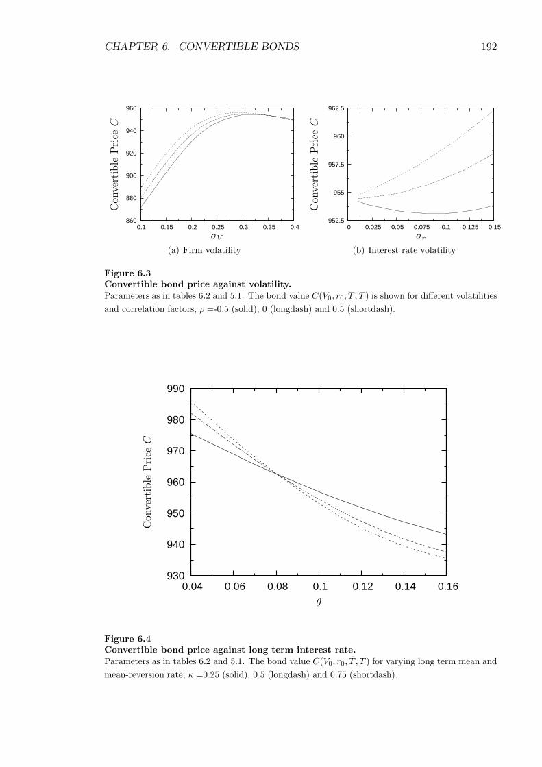
CHAPTER 6. CONVERTIBLE BONDS 192
860
880
900
920
940
960
0.1 0.15 0.2 0.25 0.3 0.35 0.4
σV
Con
vert
ible
Pri
ceC
(a) Firm volatility
952.5
955
957.5
960
962.5
0 0.025 0.05 0.075 0.1 0.125 0.15
σr
Con
vert
ible
Pri
ceC
(b) Interest rate volatility
Figure 6.3Convertible bond price against volatility.
Parameters as in tables 6.2 and 5.1. The bond value C(V0, r0, T , T ) is shown for different volatilities
and correlation factors, ρ =-0.5 (solid), 0 (longdash) and 0.5 (shortdash).
930
940
950
960
970
980
990
0.04 0.06 0.08 0.1 0.12 0.14 0.16
θ
Con
vert
ible
Pri
ceC
Figure 6.4Convertible bond price against long term interest rate.
Parameters as in tables 6.2 and 5.1. The bond value C(V0, r0, T , T ) for varying long term mean and
mean-reversion rate, κ =0.25 (solid), 0.5 (longdash) and 0.75 (shortdash).
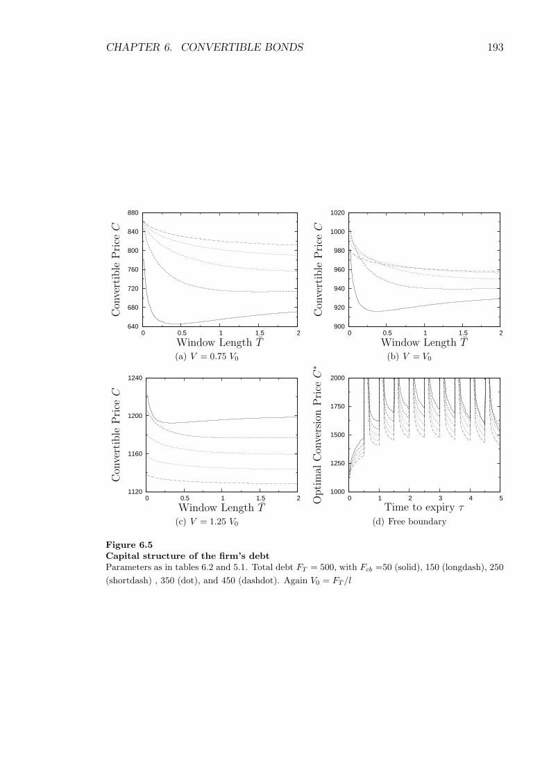
CHAPTER 6. CONVERTIBLE BONDS 193
640
680
720
760
800
840
880
0 0.5 1 1.5 2
Con
vert
ible
Pri
ceC
Window Length T(a) V = 0.75 V0
900
920
940
960
980
1000
1020
0 0.5 1 1.5 2
Con
vert
ible
Pri
ceC
Window Length T(b) V = V0
1120
1160
1200
1240
0 0.5 1 1.5 2
Con
vert
ible
Pri
ceC
Window Length T(c) V = 1.25 V0
1000
1250
1500
1750
2000
0 1 2 3 4 5
Time to expiry τ
Opti
mal
Con
vers
ion
Pri
ceC
∗
(d) Free boundary
Figure 6.5Capital structure of the firm’s debtParameters as in tables 6.2 and 5.1. Total debt FT = 500, with Fcb =50 (solid), 150 (longdash), 250
(shortdash) , 350 (dot), and 450 (dashdot). Again V0 = FT /l

CHAPTER 6. CONVERTIBLE BONDS 194
the firm becomes less and less important, all five curves converge towards the same
point. As window length is increased, the order of the firms is maintained so that
the smallest issue is the cheapest and the largest is most expensive. In figure 6.5(c),
when the firm value is relatively high, the order of the bonds has completely reversed.
Here the dilution of the firm comes into play, as the smaller issues dilute the firm
less, the conversion option on such bonds is worth more. The relative value of the
default option for these bonds is negligible at this value of the firm. However, in
figure 6.5(b), this region is a more complicated transition region as the conversion
option on the firms stock increases in price, and the probability of default decreases.
Here we see that for shorter window lengths, some of the smaller issues become more
expensive than the large issues, although the trend is eventually reversed as T → 2.
The structure of the firm would not necessarily have a large effect on the optimal
conversion of the bond since the value of the default option is usually so small for
the values of V for which we would convert. We can show that if the issue is small
enough, then the reduced dilution of the firm can lead to options where default is still
likely even for V close to conversion, since the firm value at which we convert is now
so much smaller. Figure 6.5(d) illustrates this as the small issue represented by the
solid line (Fcb=50) shows optimal conversion at smaller values than the corresponding
larger issues, for longer maturities.
Call option
The call option on a convertible bond has been extensively studied, and the results
here are standard and complement those from other studies. We present the value of
a convertible bond with a call option at facevalue. This is an extreme case although it
does present a nice boundary problem, for which the results are given in figure 6.6(b).
There are two American options now present, conversion, which attempts to maximise
the value, and a call, which attempts to minimise the value. As time tends to expiry,
the bond may be called when the interest rate is sufficiently low, or forced to convert
when the firm value is sufficiently high (so triggering the call). In the limit as time
tends to expiry, this can be expressed as when r < ccb and V > FT , or V > FT +NSScp.

CHAPTER 6. CONVERTIBLE BONDS 195
0
250
500
750
1000
1250
1500
0 500000 1e+06 1.5e+06
Con
vert
ible
Pri
ceC
Firm Value V(a)
500000
1e+06
1.5e+06
0 0.08 0.16 0.24
Interest rate r
Fir
mV
alueV
(b)
Figure 6.6Convertible bond with call option.Parameters as in tables 6.2 and 5.1. The bond is callable at face value. (a) The convertible price at
the given value of the firm with T =0.0833 (dot), 0.5 (shortdash), 1 (longdash), 2 (solid). (b) The
exercise boundary in r and V shown semi-annually over a 5 year maturity, as well as close to expiry
(solid).
The boundary as a function of V and r is shown semi-annually over a five year
maturity. We can see that for small r, for longer than around two years to maturity
the bond is no longer called. For large r, with around four years to maturity and
above the bond price is sufficiently small so that conversion is no longer forced (the
bottom three lines on the right hand side).
6.5 Conclusions
In this chapter we develop a two-factor model for convertible debt in which the
capital structure of debt in the firm is two-tier, and default is a ParAsian option. We
investigate the importance of the interest rate and its parameters on the solution, as
well as the effect of the window length of the ParAsian option on both the convertible
price and optimal conversion, over a range of leverage ratios and debt structures. The
ratio of senior debt to convertible debt is found to be important as the senior debt not
only affects the default risk of the convertible, but also conversion, since the value at
conversion is a function of the senior debt price. Varying the window length gives us
an indication of the effect of credit risk on the price. We find that the credit risk can
have a significant effect on the price, especially if the convertible debt has a smaller

CHAPTER 6. CONVERTIBLE BONDS 196
portion of total debt. We surmise that convertible bond prices need to take these
factors into account when either the firm has a low rating, or if the convertible issue
is small.

Chapter 7
A New Class of Option – The
Delayed-Exercise Option
In this chapter we propose a new type of option, motivated by a practical desire to
find an alternative to ”ruthless prepayment” used in Real Estate options work. In that
area a common assumption in the valuation of mortgages that householders perfectly
time their remortgaging activity, prepaying the moment this becomes optimal. Here,
in contrast, we model an option that requires the holder to wait a specified period of
time during which the option price is beyond a threshold before action can occur. In
order to act optimally, the holder initiates this period of waiting earlier than would
be optimal if exercise were instantaneous. This presents itself as a free boundary
problem, similar to but more complicated than the usual American option. We study
this option and those properties that give insight into the dynamics of the American
option. First, we discuss the American value process as the limiting case in which the
waiting time is zero, before discussing at length the dynamics of the delayed-exercise
option. Results are presented for a terminal as well as a perpetual option (for which
some approximations may be made), and then finally conclusions are drawn.
197
CHAPTER 7. A NEW CLASS OF OPTION 198
7.1 The American Option as a Barrier Option
As is well known, the American option has an early exercise feature, such that
the holder of the option may exercise the option at any time during the life of the
contract. For an American put, we have that
V (S, t) ≥ max[E − S, 0] (7.1)
Now, let the asset price follow a risk neutral lognormal random walk,
dS
S= r dt+ σ dW,
where dW is the risk neutral measure. Then consider the stochastic process of the
option value itself, from Ito’s lemma the process followed by V is governed by the
following equation.1
dV =
[
rS∂V
∂S+
1
2σ2S2∂
2V
∂S2+∂V
∂t
]
dt+ σS∂V
∂SdW. (7.2)
Now, the holder of the American option chooses to exercise the option when the value
of the option is at or below the exercise price, so the payoff function can be thought
to form a barrier in the option value process, at which the option itself is knocked
out. However, the exercise strategy has an effect on both the expected rate of return
on the option, (the dt term in (7.2)) and the random component, so we cannot specify
the process as such without first knowing the exercise strategy.
We also know that there exists a corresponding barrier in the asset price, the
optimal exercise boundary Sf (t), at which it is optimal to exercise below (above)
and not so above (below). This is a moving barrier, which, if hit by the asset price,
knocks out the option and the holder receives E − S. So there exists a relationship
between the option value process and its barrier, and the underlying process and its
1If the option were European, all of the partial derivatives have explicit formulae from whichthey may be calculated, so the process followed by the European option is a known function of time.

CHAPTER 7. A NEW CLASS OF OPTION 199
barrier, which can be expressed as
V (S, t) = max[E − S, 0] if S < Sf(t)
V (S, t) ≥ max[E − S, 0] if S ≥ Sf(t).
In this chapter a new framework is set down for an option where the one-touch
feature of the American option is relaxed somewhat, such that the option value has
to be below the payoff function for a prescribed amount of time before the option can
be exercised. We call this option the delayed-exercise option.
7.2 The Delayed-Exercise Option
Here we present a model where the holder of the option must initiate a ‘waiting’
period before the option can be exercised. We assume that the holder of the option
initiates this period when the value of the option is above or below the current exercise
price of the option. The option can only be exercised when the cumulative time spent
by the option value over the ‘barrier’ reaches some pre-agreed time. The Parisian
type version of the option has more financial possibilities, but mathematically is
less interesting. In this chapter, we concentrate on the nuances of the cumulative
variation, as both options have similar derivations.
Usually a barrier is crossed by the underlying asset but here we think of it as being
crossed by the option value itself. Section 7.1 described how the American option can
be regarded as a barrier option on either the option value process, or the underlying
process, as both are inextricably linked. From a framework in which the barrier is
declared in terms of the option value, we will need to find the corresponding barrier
in terms of the asset value in order to price the option
We refer back to section 4.3 for the formulation of the ParAsian option, and we
use the same notation here. In (4.17) we gave the change in barrier clock time to
be dependent on whether the asset value was above (below) some barrier H , for this

CHAPTER 7. A NEW CLASS OF OPTION 200
new option (of the ‘down’ variant), let
dt =
dt if V (S, t, t ) ≤ G(S, t)
0 if V (S, t, t ) > G(S, t), (7.3)
where G(S, t) is the barrier on the option value process. As before, we wish now to
interpret this in terms of the underlying asset. So we will require the existence of
some function in the underlying asset, H(t, t ) for which
V (S, t, t ) < G(S, t) if S < H(t, t )
V (S, t, t ) ≥ G(S, t) if S ≥ H(t, t ). (7.4)
Then it follows that we can write (7.3) as
dt =
dt if S ≤ H(t, t )
0 if S > H(t, t ), (7.5)
where the H(t, t ) is a function to be determined. We define the function H(t, t ) to
be the implied barrier since it depends on the value of the function V (S, t, t ) by (7.4),
which itself depends on the value of H(t, t ) through (7.5.) Therefore the function
H(t, t ) cannot be determined until V (S, t, t ) has been determined, so the implied
barrier creates a free boundary which needs to be determined as part of the solution.
Hence, we can reduce the problem to a ‘free’ barrier ParAsian problem, in which the
position of the implied barrier has to be found as part of the solution.
The delaying of exercise, is, in essence, a sub-optimal option, so the question is
to reason why anyone would need to model such an option. There are two main
motivations for studying such options. First, the early exercise feature is not always
the preserve of the holder. Notable exceptions are the call features in bond con-
tracts, in which the writer of the bond has the option to buy back the bond at a
predetermined amount, and also similar features on mortgage-backed securities. In

CHAPTER 7. A NEW CLASS OF OPTION 201
collaboration with the author, Sharp et al. (2007) have introduced the Parisian vari-
ant of the option into mortgage-backed securities framework, where the writer of the
option, the borrower (the holder is the bank), often chooses to delay prepayment. It
is well known that the writers of convertible bonds do not always act ‘optimally’ and
delay the calling of the bond until the stock price is above the conversion price for
some time, or alternatively, the bond value is above the call price. Gauthier (2000)
also concludes that real options are often exercised sub-optimally, or that exercise is
delayed. Second, the option can provide a fluid link between the European option
and the American option. This will be of especial interest later, when a new method
will be suggested for extrapolating from European to American values.
7.2.1 Rational Pricing
Following rational option pricing, such as that used by Merton (1990), some
bounds can be imposed on the value of the delayed-exercise option. Let VE(S, t)
be the European Option, VA(S, t) be the American equivalent, and V (S, t, t ) be the
delayed-exercise option. Given the European option and the American option with
the same parameters, it follows that
VA(S, T − t) ≥ VE(S, T − t), (7.6)
and that
VA(S, T − t1) ≥ VA(S, T − t2) if t2 ≥ t1. (7.7)
These two inequalities follow from the principle that the option to exercise, like all
options, intrinsically has positive value. For (7.6), if the holder has the right to
exercise, then he must pay for this right, since he can choose to exercise, or not to
exercise, optimally. At worst, if he never exercises, the two options are equivalent,
since he will only choose to exercise if it is optimal to do so; the value of the option
must increase if he chooses to exercise. Similarly, for (7.7) the holder of the option
with longer maturity has more time during which to exercise. If the holder of the

CHAPTER 7. A NEW CLASS OF OPTION 202
option with longer maturity, adopts an approach to convert optimally up until the
maturity date of the shorter option, at which time he unconditionally exercises, the
two options would be worth the same amount. Since the holder of the option with
longer maturity does not have to convert at the shorter ones maturity date, and
acting optimally would not necessarily do so, the longer option has more value.
For the delayed-exercise option, if the time to knock-out, T − t is longer than the
time to maturity then the option value is simply that of the corresponding European,
V (S, T − t, T − t ) = VE(S, T − t) if T − t > T − t.
At the other extreme, analogous to the manner in which the ParAsian option asymp-
totes to the vanilla barrier option as the time to knock-out reaches zero, the delayed-
exercise becomes American:
limT−t→0
V (S, T − t, T − t ) = VA(S, T − t).
Section 7.1 has already explained how an American option can be viewed as a knock-
out barrier option.
The delayed-exercise option must also satisfy
V (S, T − t, T − t1) ≥ V (S, T − t, T − t2) if T − t1 ≤ T − t2.
When the time-to-knock-out is closer, the option is worth more, because it is more
likely to be exercised (much in the same way as the American is always worth more
than the European). Hence the following inequalities between the three options can
be stated,
VE(S, T − t) ≤ V (S, T − t, T − t ) ≤ VA(S, T − t).
If we assume that the value of the delayed-exercise option is continuous across t, the
knock-out time, then the delayed option will form a continuous function linking the
European option to its American counterpart.

CHAPTER 7. A NEW CLASS OF OPTION 203
7.2.2 Pricing the delayed-exercise option
Now let us study delayed-exercise on a put option. Let the option be defined such
that
V (S, T, t) = max[E − S, 0] ∀ t, (7.8)
V (S, t, T ) = max[E − S, 0] ∀ t, (7.9)
noting that at knock-out the exchange is not for an option expiring at T , but the
exercise value. Then the condition on the barrier clock is
dt =
dt if S ≤ H(t, t )
0 if S > H(t, t ), (7.10)
where H(t, t ) is the implied barrier. Since we must solve the option as if it were a
ParAsian option with a moving barrier, then referring to section 4.3, we must solve
(4.6) for S ≤ H(t, t ), and (4.5) for S > H(t, t ). Now from (7.4), we know that the
value of the option at the barrier is given by
V (H(t, t ), t, t) = E −H(t, t ), (7.11)
since the option value must be below the payoff when the asset price is below the
barrier, and above the payoff when the asset price is above the barrier. We also need
a second condition on the barrier in order to determine the position of the barrier,
namely continuity of the first derivative across the barrier,
∂V
∂S
∣
∣
∣
∣
S=H(t,t)−
=∂V
∂S
∣
∣
∣
∣
S=H(t,t)+
. (7.12)
Let us refer back to section 7.2.1, where we have that
VE(S, T − t) ≤ V (S, T − t, T − t ) ≤ VA(S, T − t).

CHAPTER 7. A NEW CLASS OF OPTION 204
0.65
0.7
0.75
0.8
0.85
0.9
0.95
1
0 0.05 0.1 0.15 0.2 0.25 0.3 0.35
Ass
etP
riceS
Time t
Figure 7.1Monte Carlo simulation.A Monte Carlo simulation showing how the option is highly path dependent. The thin solid line
shows a random walk with S0 = 1, the thick solid line is the optimal stopping barrier Sf for an
American put, the dashed is the implied barrier H for the random walk shown. Sf is calculated
using methods from chapter 2, H is calculated by methods discussed later, with σ = 0.4, r = 0.1,
T = 0.5 and T = 0.1.
CHAPTER 7. A NEW CLASS OF OPTION 205
It then follows that for a put option, where it optimal to exercise at or below the
exercise boundary
HE(T − t) ≥ H(T − t, T − t ) ≥ Sf (T − t).
We also have that
V (S, T − t, T − t1) ≤ V (S, T − t, T − t2) if T − t1 ≥ T − t2,
from which it follows that
H(T − t, T − t1) ≤ H(T − t, T − t2) if T − t1 ≥ T − t2.
In figure 7.1, a single Monte-Carlo simulation was used to produce a risk-neutral
random-walk by the asset (solid line). Then using numerical methods described later
in this chapter, the value of option and its implied barrier were calculated. The
dashed line shows the implied barrier H(t, t ), for the given path. As the asset value
moves below the barrier, t increases, and the option is more likely to be knocked out.
This has the effect of decreasing H , therefore making it less likely to be knocked out.
For the walk shown, the delayed-exercise option from which we derive H has a knock-
out time of 0.1, the thick solid line shows Sf (T − t) for the corresponding American
option. This American option would have been knocked-out around t = 0.22, when
the asset path crosses the thick solid line. Here, exercise is delayed until t = 0.31,
when the option value has been cumulatively below the exercise price for 0.1 years.
Notice that H(t, t )→ Sf(t), as knock-out becomes more and more likely.
7.2.3 The Existence of the Implied Barrier
Now we can use the bounds imposed from section 7.2.1 to guarantee that there
exists a unique point, S such that
V (S, t, t ) = G(S, t). (7.13)
CHAPTER 7. A NEW CLASS OF OPTION 206
Let us consider a put option, as described above, with G(S, t) = E − S. The fact
that the solution is bounded above and below by VA and VE (by definition there
exists a point both on VE and VA for which (7.13) holds) implies that we can guar-
antee that there exists at least one point such that (7.13) is satisfied, and that
S ∈ ( Sf (t), HE(t) ). It can be shown that for there to exist two or more points
such that (7.13) holds, we would require that
∂V
∂S≤ −1,
for S ∈ ( Sf(t), HE(t) ). However, by rational pricing theory, the minimum value
∆ can take for a put option is −1. When hedging, the writer of the option would
never need to go long in more than one share, since that is the maximum number
of shares the writer is liable to deliver. If ∆ = −1 over some range [S∗min, S
∗max] ∈
( Sf (t), HE(t) ) such that V (S∗, t, t ) = E−S∗, then V (S, t, t ) is an American option
with optimal exercise boundary S∗max > Sf (t). So by the uniqueness of VA(S, t) such
a solution cannot exist. Similarly this type of argument can be extended to more
general options, such as a call on a stock, where ∆ ≤ 1, or a call on a bond where
∆ ≥ 0.
For the implied barrier to exist, we require that when we impose the barrier
H(t, t ), there exists a barrier such that
H(t, t ) = S (7.14)
V (S, t, t ) = E − S. (7.15)
This can be achieved by trapping the barrier. Let us apply an arbitrary barrier,
H ′ ∈ [ Sf (t), HE(t) ], at time t, t, and assume that V (S, t, t;H ′) is a continuous
function with respect to the parameter H ′. Then for a given H ′, there exists a point
in S, say S ′, such that
V (S ′, t, t;H ′) = E − S ′.
So we have that either S ′ ∈ (Sf (t), H′), S ′ ∈ (H ′, HE(t) ) or S ′ = H ′ in which case

CHAPTER 7. A NEW CLASS OF OPTION 207
H ′ = H(t, t ).
Assume that S ′ ∈ (Sf (t), H′) is now a function of the choice of barrier,2 H ′, then
by the continuity of V (S, t, t ;H ′) w.r.t. the barrier H ′, the function S ′(H ′) is also
continuous. Therefore we can always choose a value H ′min such that
S ′(H) < H ∀ H ∈ (H ′min, H
′). (7.16)
Then at the minimum value of H ′min for which (7.16) is satisfied, H ′ = S ′, which
determines the location of the implied barrier.
7.3 Numerical Analysis
In this section we outline a fixed grid method with which to solve the delayed-
exercise option. Unfortunately, the formulation of the problem does not lead to
variational inequalities, and then a linear complementarity problem (such as the one
outlined in chapter 2 for the American option), for which it would be simple to solve
using a Projected SOR algorithm. To develop a numerical scheme to price such an
option is a lot less straightforward than for the simple American option. We use
Newton iteration to find the position at which V crosses the payoff function, S ′, as
a function of H so that we can iterate until S ′ = H . The convergence of this scheme
relies on our ability to position the barrier continuously over the domain. In modelling
the ParAsian feature we follow the numerical techniques outlined in section 4.2.2.
We can then form the following set of equations for nodes not on the barrier,
αivk+1,l+1i−1 + (
1
∆τ+ βi)v
k+1,l+1i + γiv
k+1,l+1i+1 = Zk,l
i if i ≤ hk+1,l+1i ,
αivk+1,l+1i−1 + (
1
∆τ+ βi)v
k+1,l+1i + γiv
k+1,l+1i+1 = Zk,l+1
i if i > hk+1,l+1i . (7.17)
2The argument is the same if S′ ∈ (H ′, HE(t) )
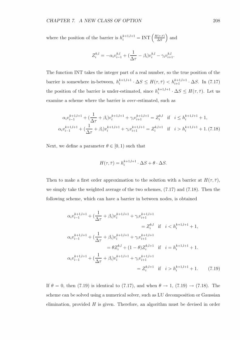
CHAPTER 7. A NEW CLASS OF OPTION 208
where the position of the barrier is hk+1,l+1i = INT
(
H(τ,τ)∆S
)
and
Zk,li = −αiv
k,li−1 + (
1
∆τ− βi)v
k,li − γiv
k,li+1.
The function INT takes the integer part of a real number, so the true position of the
barrier is somewhere in-between, hk+1,l+1i ·∆S ≤ H(τ, τ) < hk+1,l+1
i+1 ·∆S. In (7.17)
the position of the barrier is under-estimated, since hk+1,l+1i ·∆S ≤ H(τ, τ). Let us
examine a scheme where the barrier is over -estimated, such as
αivk+1,l+1i−1 + (
1
∆τ+ βi)v
k+1,l+1i + γiv
k+1,l+1i+1 = Zk,l
i if i ≤ hk+1,l+1i + 1,
αivk+1,l+1i−1 + (
1
∆τ+ βi)v
k+1,l+1i + γiv
k+1,l+1i+1 = Zk,l+1
i if i > hk+1,l+1i + 1. (7.18)
Next, we define a parameter θ ∈ [0, 1) such that
H(τ, τ) = hk+1,l+1i ·∆S + θ ·∆S.
Then to make a first order approximation to the solution with a barrier at H(τ, τ),
we simply take the weighted average of the two schemes, (7.17) and (7.18). Then the
following scheme, which can have a barrier in between nodes, is obtained
αivk+1,l+1i−1 + (
1
∆τ+ βi)v
k+1,l+1i + γiv
k+1,l+1i+1
= Zk,li if i < hk+1,l+1
i + 1,
αivk+1,l+1i−1 + (
1
∆τ+ βi)v
k+1,l+1i + γiv
k+1,l+1i+1
= θZk,li + (1− θ)Zk,l+1
i if i = hk+1,l+1i + 1.
αivk+1,l+1i−1 + (
1
∆τ+ βi)v
k+1,l+1i + γiv
k+1,l+1i+1
= Zk,l+1i if i > hk+1,l+1
i + 1. (7.19)
If θ = 0, then (7.19) is identical to (7.17), and when θ → 1, (7.19) → (7.18). The
scheme can be solved using a numerical solver, such as LU decomposition or Gaussian
elimination, provided H is given. Therefore, an algorithm must be devised in order

CHAPTER 7. A NEW CLASS OF OPTION 209
Grid search(barrier, v, g)1 theta = 02 while error > tol3 do4 ComputeScheme(alpha, beta, gamma, z, v, barrier, theta)5 TridiagonalSolver(alpha, beta, gamma, z, v)6 FindNewBarrier(newbarrier, barrier, newtheta, theta, v, g)7 error← (barrier − newbarrier)2 + (theta− newtheta)2
8 theta← newtheta9 barrier ← newbarrier
10 return nil
Figure 7.2Grid search algorithm – pseudo code
to iterate and find the barrier H . This updated scheme ensures that the solution
vk+1,l+1 is continuous with respect to the choice of the barrier.
7.3.1 The Delayed-Exercise Option Algorithm
Figure 7.2 shows the algorithm used to solve for the delayed-exercise option. The
algorithm is used to solve for each barrier timestep in turn. The inputs to the
algorithm are: the integer value hk+1,li from the previous calculation, ‘barrier’; the
value of the option at each of the four nodes needed to calculate vk+1,l+1, ‘v’; and the
constraint or exercise value G(S) = E − S, ‘g’. The function ‘ComputeScheme’ sets
up the numerical scheme as in (7.19). Then the system is solved using a tridiagonal
solver. Then we can find the position S∗, at which the solution v crosses the constraint
g. We can then calculate ‘newbarrier’ and ‘newtheta’ from
S∗ = newbarrier ⋆∆S + newtheta ⋆∆S
where ‘newbarrier’ is an integer and ‘newtheta’ is a real number in [0, 1). Then,
when the difference between the old position of the barrier and the barrier position
implied by that barrier is sufficiently small we exit the loop.
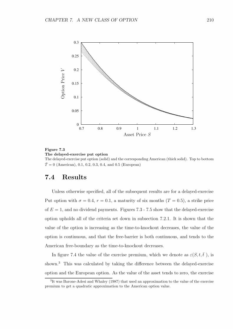
CHAPTER 7. A NEW CLASS OF OPTION 210
0
0.05
0.1
0.15
0.2
0.25
0.3
0.7 0.8 0.9 1 1.1 1.2 1.3
Opti
onP
riceV
Asset Price S
Figure 7.3The delayed-exercise put optionThe delayed-exercise put option (solid) and the corresponding American (thick solid). Top to bottom
T = 0 (American), 0.1, 0.2, 0.3, 0.4, and 0.5 (European)
7.4 Results
Unless otherwise specified, all of the subsequent results are for a delayed-exercise
Put option with σ = 0.4, r = 0.1, a maturity of six months (T = 0.5), a strike price
of E = 1, and no dividend payments. Figures 7.3 - 7.5 show that the delayed-exercise
option upholds all of the criteria set down in subsection 7.2.1. It is shown that the
value of the option is increasing as the time-to-knockout decreases, the value of the
option is continuous, and that the free-barrier is both continuous, and tends to the
American free-boundary as the time-to-knockout decreases.
In figure 7.4 the value of the exercise premium, which we denote as ε(S, t, t ), is
shown.3 This was calculated by taking the difference between the delayed-exercise
option and the European option. As the value of the asset tends to zero, the exercise
3It was Barone-Adesi and Whaley (1987) that used an approximation to the value of the exercisepremium to get a quadratic approximation to the American option value.

CHAPTER 7. A NEW CLASS OF OPTION 211
0
0.005
0.01
0.015
0.02
0.025
0.03
0.035
0.04
0.045
0.05
0.6 0.8 1 1.2 1.4
Exer
cise
Pre
miu
mε
Asset Price S
Figure 7.4The exercise premium.The value of the option to exercise (V (S, 0, 0)− VE(S, 0)) against the asset price S. The thick solid
line is the value of the American option to exercise (VA − VE). Top to bottom time-to-knockout T
is increased in steps of 0.05, from 0 (American) to 0.5 (European).

CHAPTER 7. A NEW CLASS OF OPTION 212
-0.05
-0.045
-0.04
-0.035
-0.03
-0.025
-0.02
-0.015
-0.01
-0.005
0
0.6 0.8 1 1.2 1.4
Del
aypri
ceς
Asset Price S
Figure 7.5The delay option.The value of the option to delay (V (S, 0, 0) − VA(S, t)) against the asset price S. The thick solid
line is the value of the option to wait till expiry (VE − VA). Top to bottom time-to-knockout T is
increased in steps of 0.05 from 0 (American) to 0.5 (European).
premium is given by
ε(0, t, t ) = E ·(
min[e−r(T−t ), 1]− e−r(T−t))
.
This is because when S = 0 the asset price will definitely be below the implied asset
barrier, and will either be exercised at maturity, or after T − t if T − t < T −t. As the
asset value grows without bound, the value of the option to exercise is reduced as the
probability that it will ever be under the implied barrier for T − t approaches zero.
Hence, the American, and all delayed-exercise option values approach that of the
European. Around the strike price E = 1 we can see that when the time-to-knockout
is small the growth in value of the option appears linear in t.
In figure 7.5 the option to delay exercise, denoted ς(S, t, t ) is shown. This is calcu-
lated by taking the difference between the delayed-exercise option and the American
option. The option value is negative because it is to the option writer’s advantage to
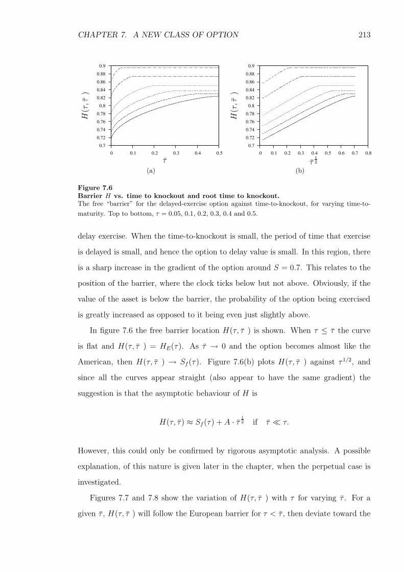
CHAPTER 7. A NEW CLASS OF OPTION 213
0.7
0.72
0.74
0.76
0.78
0.8
0.82
0.84
0.86
0.88
0.9
0 0.1 0.2 0.3 0.4 0.5
H(τ,τ
)
τ(a)
0.7
0.72
0.74
0.76
0.78
0.8
0.82
0.84
0.86
0.88
0.9
0 0.1 0.2 0.3 0.4 0.5 0.6 0.7 0.8
H(τ,τ
)
τ12
(b)
Figure 7.6Barrier H vs. time to knockout and root time to knockout.The free “barrier” for the delayed-exercise option against time-to-knockout, for varying time-to-
maturity. Top to bottom, τ = 0.05, 0.1, 0.2, 0.3, 0.4 and 0.5.
delay exercise. When the time-to-knockout is small, the period of time that exercise
is delayed is small, and hence the option to delay value is small. In this region, there
is a sharp increase in the gradient of the option around S = 0.7. This relates to the
position of the barrier, where the clock ticks below but not above. Obviously, if the
value of the asset is below the barrier, the probability of the option being exercised
is greatly increased as opposed to it being even just slightly above.
In figure 7.6 the free barrier location H(τ, τ ) is shown. When τ ≤ τ the curve
is flat and H(τ, τ ) = HE(τ). As τ → 0 and the option becomes almost like the
American, then H(τ, τ ) → Sf(τ). Figure 7.6(b) plots H(τ, τ ) against τ 1/2, and
since all the curves appear straight (also appear to have the same gradient) the
suggestion is that the asymptotic behaviour of H is
H(τ, τ) ≈ Sf(τ) + A · τ 12 if τ ≪ τ.
However, this could only be confirmed by rigorous asymptotic analysis. A possible
explanation, of this nature is given later in the chapter, when the perpetual case is
investigated.
Figures 7.7 and 7.8 show the variation of H(τ, τ ) with τ for varying τ . For a
given τ , H(τ, τ ) will follow the European barrier for τ < τ , then deviate toward the
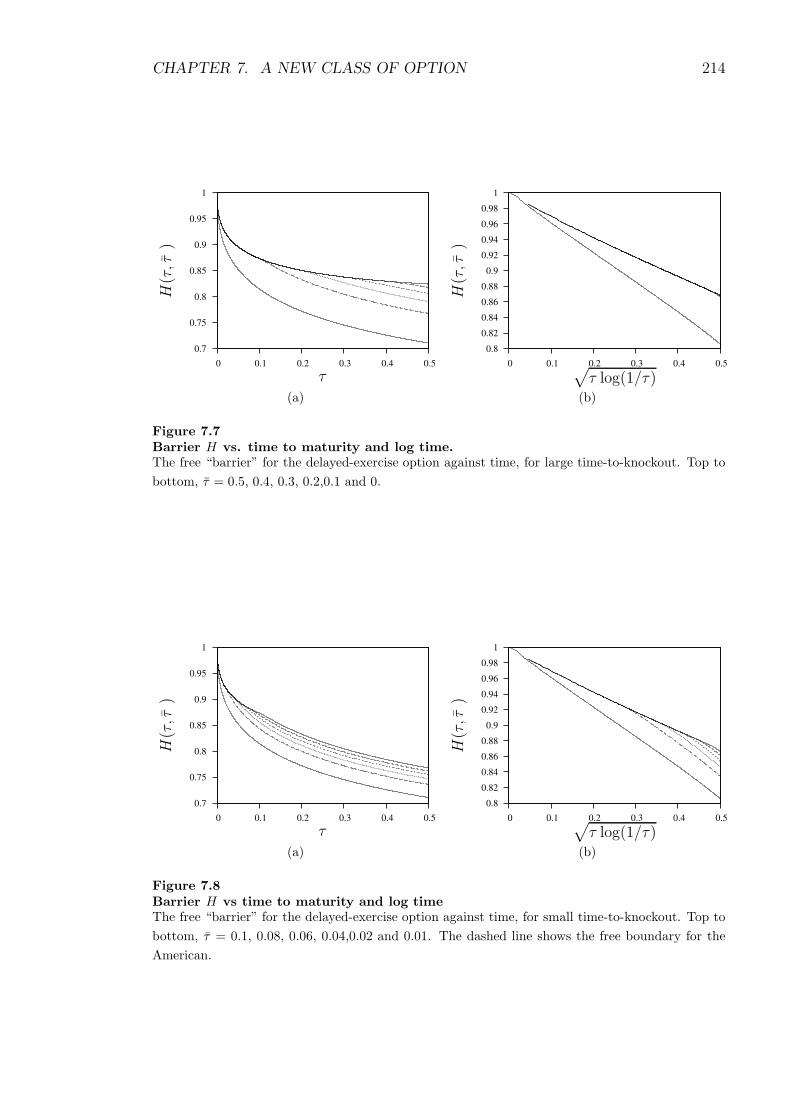
CHAPTER 7. A NEW CLASS OF OPTION 214
0.7
0.75
0.8
0.85
0.9
0.95
1
0 0.1 0.2 0.3 0.4 0.5
H(τ,τ
)
τ
(a)
0.8
0.82
0.84
0.86
0.88
0.9
0.92
0.94
0.96
0.98
1
0 0.1 0.2 0.3 0.4 0.5
H(τ,τ
)
√
τ log(1/τ)(b)
Figure 7.7Barrier H vs. time to maturity and log time.The free “barrier” for the delayed-exercise option against time, for large time-to-knockout. Top to
bottom, τ = 0.5, 0.4, 0.3, 0.2,0.1 and 0.
0.7
0.75
0.8
0.85
0.9
0.95
1
0 0.1 0.2 0.3 0.4 0.5
H(τ,τ
)
τ
(a)
0.8
0.82
0.84
0.86
0.88
0.9
0.92
0.94
0.96
0.98
1
0 0.1 0.2 0.3 0.4 0.5
H(τ,τ
)
√
τ log(1/τ)(b)
Figure 7.8Barrier H vs time to maturity and log timeThe free “barrier” for the delayed-exercise option against time, for small time-to-knockout. Top to
bottom, τ = 0.1, 0.08, 0.06, 0.04,0.02 and 0.01. The dashed line shows the free boundary for the
American.

CHAPTER 7. A NEW CLASS OF OPTION 215
-1
-0.8
-0.6
-0.4
-0.2
0
0.6 0.8 1 1.2 1.4
∆
S(a) ∆
0
0.05
0.1
0.15
0.2
0.25
0.6 0.8 1 1.2 1.4
Γ
S(b) Γ
Figure 7.9The Greeks.The value of ∆ and Γ against the asset price S for varying values of time-to-knockout for a six
month option. Top to bottom τ = 0.5 (European), 0.4, 0.3, 0.2, 0.1 and 0 (American).
American free boundary, and then seems to stay parallel to it. It has been shown
earlier (section 2.3) that for small τ the free boundary of the American put will be
of order√
τ log(1/τ). Then in figures 7.7(b) and 7.8(b) the free barrier is plotted
against√
τ log(1/τ). The American free boundary forms a straight line, as does
the European barrier. When τ is small H also forms a straight line parallel to the
American free boundary. This suggests that H is of order√
τ log(1/τ) in τ when
τ ≫ τ . Again though, these graphs cannot confirm these trends, and future work
could involve investigating the asymptotic analysis of such a problem.
Figures 7.9 and 7.10 plot the Greeks ∆ and Γ for various τ . Figure 7.10(a) shows
how the ∆ for the European option converges as τ → 0 to the ∆ for the American.
The ∆ for the American is undefined for S < Sf (t) since the option has been exercised,
but we take it to be -1 here. This causes an apparent discontinuity in Γ, but the
option is undefined in this region so it does not really exist. The discontinuity is
transferred to the delayed-exercise Γ, at the barrier level H(τ, τ ). ∆ is continuous
across the barrier though, and in figure 7.10(a) it can be seen how ∆ follows the
hedging strategy for the American when S > H and one that resembles a European
(with time-to-maturity equal to the time-to-knockout) when S < H . It is this change
in strategy across the barrier that causes the discontinuity in Γ.
In fact, we can use the continuity across the barrier to give us a smooth pasting

CHAPTER 7. A NEW CLASS OF OPTION 216
-1
-0.99
-0.98
-0.97
-0.96
-0.95
-0.94
-0.93
-0.92
-0.91
-0.9
0.66 0.68 0.7 0.72 0.74
∆
S(a) ∆
0
0.05
0.1
0.15
0.2
0.25
0.66 0.68 0.7 0.72 0.74
Γ
S(b) Γ
Figure 7.10The Greeks, zoomed region.The value of ∆ and Γ against the asset price S for varying small values of time-to-knockout for a
six month option. Top to bottom τ = 0.01, 0.005 and 0 (American).
condition, just as we have for the standard American option. The continuity of ∆
ensures that a solution is consistent and satisfies the BSM equation. For the American
option, the constraint says that the value of the option must always be greater than
or equal to the exercise price. However, when the problem is formulated using the
free-boundary condition, the constraint is hidden inside the smooth pasting condition:
V (S, t) > G(S) ⇐⇒ V (Sf , t) = G(Sf) and VS(Sf , t) = GS(Sf).
Similarly, we can formulate the delayed-exercise option using a smooth pasting con-
dition:
V (S, t, t ) < E −H(t, t) if S < H(t, t)
and V (S, t, t ) > E −H(t, t) if S > H(t, t),
⇐⇒ V (H(t, t ), t, t ) = E −H(t, t)
and VS(H(t, t )−, t, t ) = VS(H(t, t )+, t, t ). (7.20)
When studying the option value it has been previously commented that the option
value appears to tend toward the American option value in a linear fashion. If this is
the case, this may lead to a means of extrapolating from the European value to the
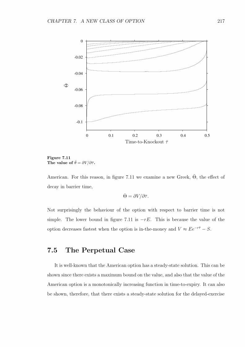
CHAPTER 7. A NEW CLASS OF OPTION 217
-0.1
-0.08
-0.06
-0.04
-0.02
0
0 0.1 0.2 0.3 0.4 0.5
Θ
Time-to-Knockout τ
Figure 7.11The value of θ = ∂V/∂τ .
American. For this reason, in figure 7.11 we examine a new Greek, Θ, the effect of
decay in barrier time,
Θ = ∂V/∂τ .
Not surprisingly the behaviour of the option with respect to barrier time is not
simple. The lower bound in figure 7.11 is −rE. This is because the value of the
option decreases fastest when the option is in-the-money and V ≈ Ee−rτ − S.
7.5 The Perpetual Case
It is well-known that the American option has a steady-state solution. This can be
shown since there exists a maximum bound on the value, and also that the value of the
American option is a monotonically increasing function in time-to-expiry. It can also
be shown, therefore, that there exists a steady-state solution for the delayed-exercise

CHAPTER 7. A NEW CLASS OF OPTION 218
option. From the rational pricing discussed earlier,
V (S, τ1, τ) > V (S, τ2, τ) if τ1 > τ2 and τ2 ≥ τ ,
shows the function is monotonically increasing in τ for τ > τ , and we have the upper
bound
V (S, τ, τ ) < VA(S, τ) if τ > 0.
Then there must exist a steady state solution. So let us set ∂/∂τ = 0 in (4.6) and
(4.5) to obtain
Vτ =1
2σ2S2VSS + rSVS − rV for S < H(τ) (7.21)
0 =1
2σ2S2VSS + rSVS − rV for S > H(τ), (7.22)
subject to the following boundary conditions;
V (S, 0) = max[E − S, 0], (7.23)
V (0, τ) = E · e−rτ , (7.24)
V (H(τ), τ) = E −H(τ), (7.25)
∂V
∂S
∣
∣
∣
∣
S=H(τ)−
=∂V
∂S
∣
∣
∣
∣
S=H(τ)+
, (7.26)
V (∞, τ) = 0. (7.27)
Let us examine (7.22), which can be solved analytically using a solution of the
Euler type. Assume a solution of the Euler type, then
V (S, τ) = A Sα,
and on substituting into (7.22) we obtain
1
2σ2α(α− 1) + rα− r,

CHAPTER 7. A NEW CLASS OF OPTION 219
from which
α = −2r
σ2or α = 1.
From (7.27) we deduce that α = − 2rσ2 is the correct root, and apply the boundary
condition (7.25) to obtain
V (S, τ) =E −H(τ)
H(τ)αSα (7.28)
This solution, for a given value of H(τ), will have a value for the first derivative,
which will feed into (7.21) via the boundary condition (7.26). Hence, (7.21) must be
solved numerically, subject to the boundary conditions
V (S, 0) = max[E − S, 0] (7.29)
V (0, τ) = E · e−rτ (7.30)
V (H, τ ) = E −H (7.31)
∂V
∂S
∣
∣
∣
∣
S=H
= αE −HH
. (7.32)
This is similar to the free-boundary formulation for a American option, and just as
in that case an extra condition for the initial value of the free boundary is required.
It has already been shown that the free-barrier H tends toward the free-boundary Sf
when τ → 0, so
H(0) =αE
α− 1. (7.33)
7.5.1 Asymptotic analysis – in the limit as time-to-knockout
tends to zero
Making the substitutions S = Eex, τ = τ /12σ2, and V (S, τ) = E−S+Ee−ρτv(x, τ)
into (7.21), the result is
∂v
∂τ=∂2v
∂x2+ (ρ− 1)
∂v
∂x− ρeρτ (7.34)

CHAPTER 7. A NEW CLASS OF OPTION 220
subject to the boundary conditions
v(x, 0) = 0,
v(−∞, τ) = 1− eρτ ,
v(xf , τ) = 0,
∂v
∂x
∣
∣
∣
∣
x=xf
= ρeρτ (exf − 1) + exf +ρτ ,
x0 = log
(
ρ
ρ+ 1
)
,
where H(0) = Eex0.
Let us study the behaviour of the solution in the knockout limit. Let τ = ǫT
where T = O(1) and ǫ is a small parameter. Then we have the following PDE,
∂v
∂T= ǫ
[
∂2v
∂x2+ (ρ− 1)
∂v
∂x− ρeǫρT
]
(7.35)
So let us look for an asymptotic solution of the form
v(x, τ) = V0(x, T ) + ǫV1(x, T ) +O(ǫ2) (7.36)
Then the O(1) approximation is just zero, and to O(ǫ) we have
∂V1
∂T(x, T ) = 0, (7.37)
then subject to the transformed boundary condition we have the following expansion
for v in the region x < x0.
v(x, τ) = −ρτ +O(ǫ2).
This solution matches neither of the boundary conditions at x0, so we need to intro-
duce a new scaling to the problem.
Let us define a separate region close to the free boundary, and introduce the

CHAPTER 7. A NEW CLASS OF OPTION 221
following scalings
x = x0 + ǫ12X, V = ǫV xf = x0 + ǫ
12L0.
Then
∂V
∂T=∂2V
∂X2+ ǫ
12 (ρ− 1)
∂V
∂X− ρ(1 + ǫρT ) +O(ǫ
32 ), (7.38)
and to first order we obtain
∂V
∂T=∂2V
∂X2− ρ, (7.39)
with boundary conditions
V (L0, T ) = 0, (7.40)
∂V
∂X(L0, T ) = ρL0, (7.41)
V → −ρT as x→ −∞, (7.42)
where the last condition is a matching condition for the expansion. Then seek a
similarity solution of the form V = τ g(ξ) where ξ = X/√
T , and L0 = ξ0√
T , to
arrive at the following ODE;
g′′ +1
2ξg′ − g = ρ, (7.43)
with boundary conditions
g(ξ0) = 0, (7.44)
g′(ξ0) = −ρξ0, (7.45)
g ∼ −ρ as ξ → −∞. (7.46)
This ODE matches both of the boundary conditions at the free boundary.

CHAPTER 7. A NEW CLASS OF OPTION 222
7.5.2 Solution to the ODE
First, we start by seeking a simple polynomial solution to the homogeneous equa-
tion. Try a solution of the form
g(ξ) = a+ bξ + cξ2 + dξ3, (7.47)
which on substitution into (7.43) and equating coefficients gives a = 1, b = 0, c = 12,
and d = 0. Then a solution to the homogeneous equation is
g(ξ) = B
(
1 +1
2ξ2.
)
To find the general solution to the homogeneous equation we apply the method of
reduction of order to our solution. After some laborious algebra we arrive at
g = A.
{(
1 +1
2ξ2
)∫ ξ
−∞e−
14s2
ds+ ξe−14ξ2
}
+B
{
1 +1
2ξ2
}
, (7.48)
which is the general solution to the homogeneous ODE. The general solution to
(7.43) is the general solution of the homogeneous plus the particular solution, which
fortunately is easy to spot (gp = −ρ). Then the general solution is
g = A.
{(
1 +1
2ξ2
)∫ ξ
−∞e−
14s2
ds+ ξe−14ξ2
}
+B
{
1 +1
2ξ2
}
− ρ . (7.49)
Now we must apply the boundary conditions. From (7.46) it is obvious that
B = 0. That leaves us with two equations to find ξ0 and A. The first boundary
condition (7.44) implies that
A.
{(
1 +1
2ξ20
)∫ ξ0
−∞e−
14s2
ds+ ξ0e− 1
4ξ20
}
= ρ,
and (7.45) that
A
(
ξ0
∫ ξ0
−∞e−
14s2
ds+ 2e−14ξ20
)
= ρξ0.
Using simple algebra we find that the transcendental equation for the free boundary

CHAPTER 7. A NEW CLASS OF OPTION 223
is
ξ30e
14ξ20
∫ ξ0
−∞e−
14s2
ds = 2(2− ξ20), (7.50)
and the constant A is found via
A =ρ(1− 1/2ξ2
0)∫ ξ0−∞ e−
14s2ds
.
This is the same transcendental equation as that arrived at by Wilmott et al.
(1995) for the case of the American call with d < r. This is quite interesting since
both the ODE and the boundary conditions differ from that case. However, it does
mean that the solution has already been found for ξ0, Wilmott et al. (1995) state the
value to be
ξ0 = 0.9034 . . . .
Using Newton iteration a more accurate value can be found,
ξ0 = 0.9034466 . . . .
Hence we have found an approximation to the perpetual delayed-exercise option close
to knockout.
In the original variables we can express the free barrier to be
H(τ) = Eα
α− 1
(
1 + ξ0
√
1
2σ2τ + . . .
)
In figure 7.12 the asymptotic results are shown against the numerical results.
Since we are only interested in the premium that the option to delay exercise from
instantaneous, we look at the price difference between the American option and
the delayed-exercise option. Figure 7.12(b) plots the value of the option to delay
exercise, and figure 7.12(a) the corresponding barrier. It is clear that even a small
miscalculation of the barrier can lead to large errors in the pricing of the option.
Above the barrier, the value is analytic, so no numerical errors are present and the
only error comes from the placement of the barrier. So even though the asymptotic

CHAPTER 7. A NEW CLASS OF OPTION 224
5.6
6
6.4
0 0.1 0.2 0.3 0.4 0.5
Bar
rierH
(τ)
Time-to-Knockout τ(a)
-0.5
-0.4
-0.3
-0.2
-0.1
0
4 5 6 7 8
Asset Value S
V∗ (S,τ
)
(b)
Figure 7.12Asymptotic approximation to the perpetual caseParameters are r = 0.1, σ = 0.4 and E = 10. (a) The free barrier H(τ ) vs. time to knockout, with
the numerical value given by the dashed line, the approximation by the solid line. (b) V ∗(S, τ ) =
V (S, τ ) − VA(S) is the value of the option to delay. From top to bottom, τ = 0 through to 0.5,
with increments of 0.1.
approximation is very good below the barrier, the resulting errors on the right hand
side are large (due to the misplacement of the free barrier). The derivative around
the barrier is fast changing so the second order approximation we have taken is not
accurate enough to keep down the errors to the right of the barrier. It is to be noted
that the pricing of the option for S > H is more important since this is the region
where most if not all of these options would be sold.
7.6 Advanced Body-Fitted Solver for the Delayed-
Exercise Option
The scheme outlined earlier in section 7.3 is at best a crude attempt at a solution
to the delayed-exercise option. When reviewing the results, the extra smooth-pasting
condition at the free-barrier came to light, with which we can formulate the problem
as a pair of coupled PDEs linked by the continuity of both the option value and its
∆. The region S > H(τ, τ ) can be solved in the same way as an American put, using
the advanced body-fitted coordinate scheme with an appropriate upper boundary as
explained in Chapter 2.

CHAPTER 7. A NEW CLASS OF OPTION 225
Let W define the solution above to barrier, for which the barrier clock does not
tick. In the same manner as before, the upper boundary U , is chosen to be a function
of time so that the value of W is approximately zero. Then we choose U = Eeξσ√
τ .
The PDE (4.6) becomes
Wτ −1
G(SGτ + Fτ )WS =
1
2σ2
(
S +F
G
)2
WSS + r
(
S +F
G
)
WS − rW. (7.51)
where S = S−FG
.
For S < H(τ, τ ), the boundary conditions suggest an American style call option,
and it can be solved in the same way. We assume that V defines the solution below
the barrier, resulting in the following PDE to solve for V ,
Vτ + Vτ −Fτ + Fτ
FSVS =
1
2σ2S2VSS + rSVS − rV, (7.52)
where S = SF
.
The boundary conditions ensure the continuity of the option value and its first
derivative. Similarly, just as the perpetual option required a boundary condition
for F at knockout, so does the non-perpetual option. It has been shown that this
is the American free boundary, the limit of H as time-to-knockout tends to zero,
which means that the American option will need to be calculated in order to obtain
Sf , before we can calculate the value of the delay-exercise option. This is where
the highly accurate ABFC solver is required, in order to position the American free
boundary accurately even near expiry. Incorrect positioning could cause errors that
may contaminate the entire solution. The option value above and below the barrier

CHAPTER 7. A NEW CLASS OF OPTION 226
must be solved simultaneously subject to the following boundary conditions;
F (0, τ) = min
[
rE
d,E
]
, (7.53)
F (τ, 0) = Sf (τ), (7.54)
V (S, τ, 0) = E − (SF ), (7.55)
W (S, τ, 0) = max[E − (SG+ F ), 0], (7.56)
Vτ + Vτ + rV = 0 for S = 0, (7.57)
V (1, τ, τ) = W (0, τ, τ) = E − F (τ), (7.58)
1
F
∂V
∂S
∣
∣
∣
∣
S=1
=1
G
∂W
∂S
∣
∣
∣
∣
S=0
, (7.59)
W (1, τ, τ) = 0, (7.60)
G(τ, τ) + F (τ, τ) = U(τ). (7.61)
If we have n nodes below the barrier, and m nodes above, we have n + m + 2
equations. The two extra equations are required to find F and G and to ensure
that the solutions match at the boundary. When we are above the barrier, we can
discretise the problem and linearise using the Newton method (c.f. section 2.5) to
arrive at
αj,2(δWj−1) + βj,2(δWj) + γj,2(δWj+1) + θn+1+j(δF ) + φj(δG) = ǫn+1+j, (7.62)
where 1 < j < m. There are terms present for both F and G. The counter for θ
starts at n+1 since there are N equations for V and one equation linking V and W .
When below the barrier, we discretise setting ∆τ = ∆τ for reasons outlined in
Chapter 4. Then
Vτ (S, τ + 1/2∆τ, τ + 1/2∆τ)+ Vτ (S, τ + 1/2∆τ, τ + 1/2∆τ)
= 1∆τ
(vk+1,l+1i − vk,l
i ), (7.63)
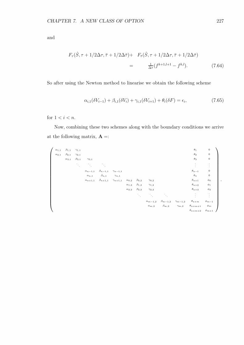
CHAPTER 7. A NEW CLASS OF OPTION 227
and
Fτ (S, τ + 1/2∆τ, τ + 1/2∆τ)+ Fτ (S, τ + 1/2∆τ, τ + 1/2∆τ)
= 1∆τ
(fk+1,l+1 − fk,l). (7.64)
So after using the Newton method to linearise we obtain the following scheme
αi,1(δVi−1) + βi,1(δVi) + γi,1(δVi+1) + θi(δF ) = ǫi, (7.65)
for 1 < i < n.
Now, combining these two schemes along with the boundary conditions we arrive
at the following matrix, A =:
α1,1 β1,1 γ1,1 θ1 0
α2,1 β2,1 γ2,1 θ2 0
α3,1 β3,1 γ3,1 θ3 0
...
...
...
.
.
.
.
.
.
αn−1,1 βn−1,1 γn−1,1 θn−1 0
αn,1 βn,1 γn,1 θn 0
αn+1,1 βn+1,1 γn+1,1 α0,2 β0,2 γ0,2 θn+1 φ0
α1,2 β1,2 γ1,2 θn+2 φ1
α2,2 β2,2 γ2,2 θn+3 φ2
...
...
...
.
.
.
.
.
.
αm−1,2 βm−1,2 γm−1,2 θn+m φm−1
αm,2 βm,2 γm,2 θn+m+1 φm
θn+m+2 φm+1
.
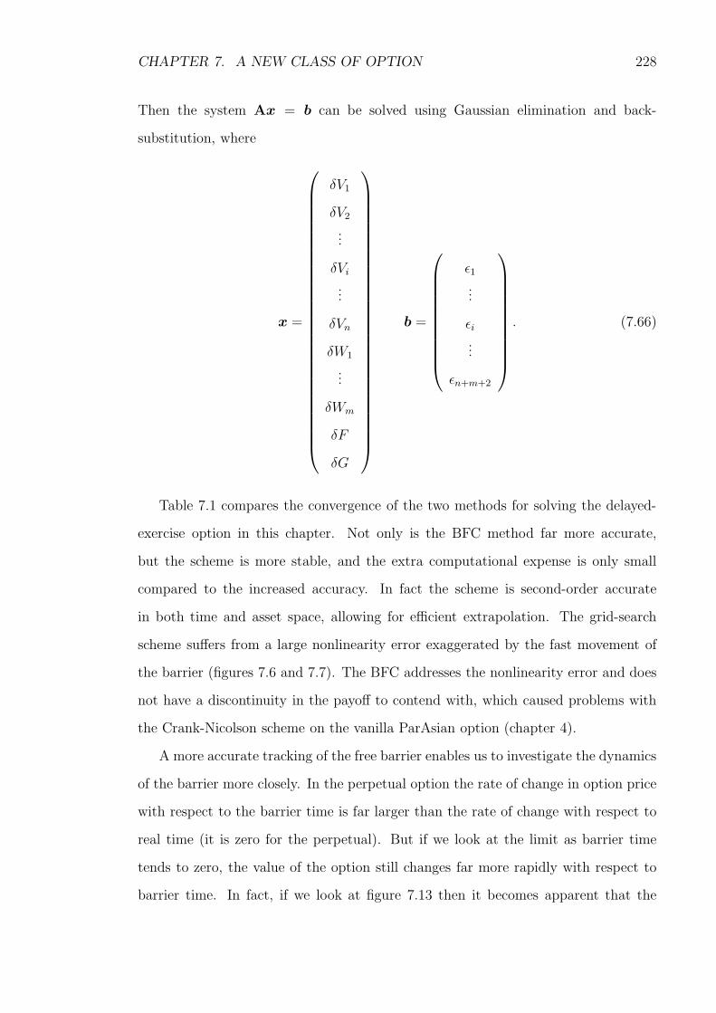
CHAPTER 7. A NEW CLASS OF OPTION 228
Then the system Ax = b can be solved using Gaussian elimination and back-
substitution, where
x =
δV1
δV2
...
δVi
...
δVn
δW1
...
δWm
δF
δG
b =
ǫ1...
ǫi...
ǫn+m+2
. (7.66)
Table 7.1 compares the convergence of the two methods for solving the delayed-
exercise option in this chapter. Not only is the BFC method far more accurate,
but the scheme is more stable, and the extra computational expense is only small
compared to the increased accuracy. In fact the scheme is second-order accurate
in both time and asset space, allowing for efficient extrapolation. The grid-search
scheme suffers from a large nonlinearity error exaggerated by the fast movement of
the barrier (figures 7.6 and 7.7). The BFC addresses the nonlinearity error and does
not have a discontinuity in the payoff to contend with, which caused problems with
the Crank-Nicolson scheme on the vanilla ParAsian option (chapter 4).
A more accurate tracking of the free barrier enables us to investigate the dynamics
of the barrier more closely. In the perpetual option the rate of change in option price
with respect to the barrier time is far larger than the rate of change with respect to
real time (it is zero for the perpetual). But if we look at the limit as barrier time
tends to zero, the value of the option still changes far more rapidly with respect to
barrier time. In fact, if we look at figure 7.13 then it becomes apparent that the

CHAPTER 7. A NEW CLASS OF OPTION 229
Table 7.1Relative RMS errors for delayed-exercise put options
n Grid-search BFC(time) (time)
200 0.002556 0.000061535(0.2) (0.4)
400 0.000425 0.000013032(1.4) (3.2)
600 0.000391 0.000007195(4.9) (10.3)
800 0.000363 0.000004733(11.6) (23.8)
1000 0.000326 0.00000327(22.9) (45.3)
1200 0.000292 0.00000237(39.6) (76.7)
1400 0.000263 0.00000175(63.1) (119.8)
1600 0.000239 0.00000131(94.3) (175.5)
1800 0.000218 0.00000097(134.) (245.3)
2000 0.000201 0.00000072(183.2) (331.9)
The relative errors for the two methods described in this chapter. The relative RMS errors are
calculated against exact values of close to 100 different put options with T = 0.5/1, S0 ∈ [0.8E, 1.2E],
σ = 0.4/0.2. For all options r = 0.06 and E = 10. The exact values are calculated by allowing
n → ∞ until successive solutions are sufficiently close to one another (1.E-8). We use n nodes
in S, results are extrapolated once using n and n/2, and the number of timesteps is n and n/2
respectively. We set ∆τ = ∆τ as usual.
behaviour of the barrier with small time to knockout mirrors the behaviour of the
perpetual barrier with small time to knockout.
In fact, from this we can make an estimate of the free boundary for the American.
By taking the point at which the European option crosses the exercise price, HE ,
then we can form an approximation to the free boundary for the American option
S∗f , simply as
S∗f (τ) = HE(τ)(1 + ξ0
√
1
2σ2τ) (7.67)
The approximation, as shown in figure 7.14 is not as accurate as was hoped for,

CHAPTER 7. A NEW CLASS OF OPTION 230
6.8
7
7.2
7.4
7.6
7.8
8
8.2
8.4
8.6
0 0.1 0.2 0.3 0.4 0.5
Bar
rierH
(τ,τ
)
Time-to-knockout τ
Figure 7.13Asymptotic H(τ, τ ) vs. time to knockoutA guess at the asymptotic form of H(τ, τ ) for small barrier time. The straight line is the numerical
result form the body-fitted solver and the dashed line the analytical approx from the perpetual case.
6
6.5
7
7.5
8
8.5
9
9.5
10
0 0.05 0.1 0.15 0.2 0.25 0.3 0.35 0.4 0.45 0.5
Bar
rierH
(τ,τ
)
Time-to-maturity τ(a)
5
5.5
6
6.5
7
7.5
0 0.05 0.1 0.15 0.2 0.25 0.3 0.35 0.4 0.45 0.5
Bar
rierH
(τ,τ
)
Time-to-maturity τ(b)
Figure 7.14Free boundary approximation S∗
f (τ) vs. time to maturity
The approximation to the free boundary (dashed) along with the exact value calculated numerically
(solid). (a) E = 10, r = 0.06, d = 0 and top to bottom σ = 0.1, 0.2, 0.4 (b) E = 10, r = 0.06,
d = 0.08 and top to bottom σ = 0.1, 0.2, 0.4
CHAPTER 7. A NEW CLASS OF OPTION 231
although further accuracy may be possible if the expansion for the perpetual option is
taken to the next term. Now this does seem rather hand wavy as an approximation,
but it does agree to some extent with Evans et al. (2002) and Widdicks et al. 2005.
Both find that there is a region of order O(τ12 ) around the free boundary. In effect,
under the framework of the delayed option, we have inadvertently set up an equation
to solve this region.
7.7 Conclusions
The delayed-exercise option proposed in this chapter is interesting as a mathe-
matical problem providing a fluid link between the European and American options.
Studying the perpetual option we can make some approximation to both the free
barrier and the option value. Two new methods are created to deal with an option
which is highly path (and strategy) dependent. It is not immediately obvious how one
could solve such a problem with any other method other than finite difference. For
a useful modeling tool however, we must look to the Parisian style delayed-exercise
option. The analysis and implementation of such an option is left to further research.

Chapter 8
Conclusions
Under the assumptions of the BSM framework, early-exercise and occupation-
time options are investigated in detail. Exploiting the asymptotic behaviour of early-
exercise options, we are able to enhance current numerical techniques with improved
convergence and efficiency. The resulting scheme is more than 2000 times as accurate
as the benchmark finite-difference scheme (PSOR), for same order computation times.
An investigation of finite-difference methods for occupation-time derivatives rules
out the use of certain methods under certain conditions. Noting some of the problems
caused by the smoothness of the solution, a new occupation time derivative, the
integral time Parisian/ParAsian option, is proposed which is at least C2 continuous.
This option has implications for the hedging of occupation-time derivatives.
These advanced techniques are then applied to corporate bonds in a complex
capital structure, where the firm issues subordinate bonds. Under the Yu (2004)
model, default under chapter 11 is modelled as a ParAsian option, the firm is allowed
to issue new debt while the APR may also be violated. A parameter analysis is
carried out over a range of maturity and debt structures to present a comprehensive
term structure of credit spreads. The model is then further advanced so that the
subordinate issue may now be convertible. The effect of the size senior issue present
is analysed.
The unique shapes that the term structure of credit spreads exhibit when the firm
issues subordinate bonds has important implications for the modelling of corporate
232
CHAPTER 8. CONCLUSIONS 233
bonds. The relative weight of senior to junior debt is found to be important in
determining the positioning of the default barrier, and also the effect that APR
violations have on the results. The weighting of senior to junior debt is also found to
be important when modelling convertible debt, as it effects both the credit spread of
the bond and dilution of shares in the firm.
The Yu (2004) model may be extended further to include the leverage ratio as a
state variable, allowing the accretion of debt to be dependent on the position in the
state space rather than a constant as given in this thesis. It may also be possible to
include the barrier as a state variable, or at least solve to find the optimum barrier
level, although this would require the inclusion of taxes and other modelling assump-
tions. A vital test for the Yu (2004) model would be to test it empirically against
other models, allowing the inclusion of firms with multiple debt issues. Similarly
the convertible bond model must also be tested against other models to validate the
findings.
The early-exercise and occupation-time derivatives are combined to propose the
delayed-exercise option. The problem presents itself as a complex free boundary
problem, which requires the highly accurate numerical techniques developed earlier
in the thesis to be solved comprehensively, by the efficient use of finite-difference
techniques, but would be difficult to solve via other methods, due to the complex
feedback of the option value on to the solution. The solution to the simple delayed-
exercise put also sheds light on some of the intricacies of the American put option.
The delayed-exercise option has a range of interesting modelling applications,
such mortgage-backed securities, convertible bonds or real options. All of these areas
require further research on their application.

Appendix A
Numerical Schemes
A.1 BFC and ABFC coefficients
The ABFC PDE is more general, and can be reduced to the BFC PDE by appro-
priate settings of the functions F and G, so we present the coefficients for that only.
The equation is:
Vτ −1
G(SGτ + Fτ )VS =
1
2σ2
(
S +F
G
)2
VSS + r
(
S +F
G
)
VS − rV, (A.1)
with either three or four boundary conditions, depending on whether F and G are
known, resulting in n+ 1 or n+ 2 equations. The problem is discretised so that:
∆S =1
n, ∆τ =
1
m,
and
uki = V (i∆S, k∆τ),
fk = F (k∆τ), gk = G(k∆τ).
234

APPENDIX A. NUMERICAL SCHEMES 235
The coefficients when neither F nor G are known, corresponding to (2.98), are
αi = (gtSi + ft)1
4gg∆S− σ2 ss2
i
4∆S2+ (r − d) ssi
4∆S(A.2)
βi =1
∆τ+ σ2 ss2
i
2∆S2+
1
2r (A.3)
γi = −(gtSi + ft)1
4gg∆S− σ2 ss2
i
4∆S2− (r − d) ssi
4∆S(A.4)
θi = − 1
∆τ
vsi
gg− σ2ssi
ggvssi − (r − d)vsi
gg(A.5)
φi = ((gtSi + ft)1
2gg− Si
∆τ)vsi
gg+ σ2ff
ssi
2gg2vssi + (r − d)ff vsi
2gg(A.6)
ǫi = −vti + (gtSi + ft)vsi/gg +1
2σ2ss2
i vssi + (r − d)ssivsi − rvi , (A.7)
where
∂F
∂τ= ft = (fk+1 − fk)
1
∆τ(A.8)
F (τ + 1/2∆τ) = ff =1
2(fk + fk+1) (A.9)
∂G
∂τ= gt = (gk+1 − gk)
1
∆τ(A.10)
G(τ + 1/2∆τ) = gg =1
2(gk + gk+1), (A.11)
and
Si
G(τ + 1/2∆τ)= ssi = Si +
ff
gg(A.12)
∂V
∂τ= vti = (uk+1
i − uki )
1
∆τ(A.13)
V (S, τ + 1/2∆τ) = vvi =1
2(uk
i + uk+1i ) (A.14)
∂V
∂S(S, τ + 1/2∆τ) = vsi = (uk
i+1 + uk+1i+1 − uk
i−1 − uk+1i−1 )
1
4∆S(A.15)
∂2V
∂S2(S, τ + 1/2∆τ) = vssi = (uk
i+1 + uk+1i+1 − 2uk
i − 2uk+1i + uk
i−1 + uk+1i−1 )
1
2∆S2.
(A.16)

APPENDIX A. NUMERICAL SCHEMES 236
If either F or G are known, we simple set θi or φi to zero and all other terms remain
the same. Hence the BFC for the put is a special case of the ABFC where
G = F + aE
where a is a constant and E is the strike price.

References
Acharya, V. V. and Carpenter, J. N. (2002). Corporate Bond Valuation and Hedging
with Stochastic Interest Rates and Endogenous Bankruptcy, Review of Financial
Studies 15(5): 1355–1383.
Altman, E. I. (1993). Evaluating the Chapter 11 Bankruptcy-Reorganization Process,
in E. I. Altman (ed.), Bankruptcy, Credit Risk, and High Yield Junk Bonds,
Blackwells. 2002.
Amin, K. I. (1991). On the Computation of Continuous Time Option Prices Using
Discrete Approximations, The Journal of Financial and Quantitative Analysis
26(4): 477–495.
Anderluh, J. and van der Weide, H. (2004). Parisian Options – The Implied Barrier
Concept. International Conference of Computer Science.
Andersen, L. and Broadie, M. (2004). Primal-Dual Simulation Algorithm for Pricing
Multidimensional American Options, Management Science 50(9): 1222–1234.
Andricopoulos, A. D., Widdicks, M., Duck, P. W. and Newton, D. P. (2003). Universal
Option Valuation using Quadrature Methods, Journal of Financial Economics
67: 447–471.
Andricopoulos, A., Widdicks, M., Duck, P. W. and Newton, D. (2004). Curtailing the
Range for Lattice and Grid Methods, The Journal of Derivatives 11(4): 55–61.
Andricopoulos, A., Widdicks, M., Newton, D. P. and Duck, P. (2007). Extending
237

REFERENCES 238
Quadrature Methods to Value Multi-Asset and Complex Path Dependent Op-
tions, Journal of Financial Economics 83(2): 471– 499.
Avellaneda, M. and Wu, L. (1999). Pricing Parisian-Style Options with a Lattice
Method, International Journal of Theoretical and Applied Finance 2: 1–16.
Ayache, E., Forsyth, P. and Vetzal, K. (2003). The Valuation of Convertible Bonds
with Credit Risk, Journal of Derivatives 11(1): 9–29.
Barone-Adesi, G. and Whaley, R. E. (1987). Efficient Analytical Approximation of
American Option Values, The Journal of Finance 42(2): 301–320.
Bensoussan, A. (1984). On the Theory of Option Pricing, Acta Applicandae Mathe-
maticae 2(2): 139–158.
Bermudez, A. and Webber, N. (2004). An Asset Based Model of Defaultable Convert-
ible Bonds with Endogenised Recovery. Working paper, City University, Cass
Business School, London.
Bernard, C., Le Courtois, O. and Quittard-Pinon, F. (2005). A New Procedure for
Pricing Parisian Options, The Journal of Derivatives 12(4): 45–53.
Black, F. and Cox, J. (1976). On the Pricing of Corporate Debt: The Risk Structure
of Interest Rates, The Journal of Finance 29: 449–470.
Black, F. and Scholes, M. (1973). The Pricing of Options and Corporate Liabilities,
The Journal of Political Economy 81(3): 637–654.
Blanco, R., Brennan, S. and Marsh, I. W. (2005). An Empirical Analysis of the
Dynamic Relation between Investment-Grade Bonds and Credit-Default Swaps,
The Journal of Finance 60: 2255–2281.
Boyle, P. P. (1977). Options: A Monte Carlo Approach, Journal of Financial Eco-
nomics 4(3): 323–338.
Boyle, P. P. (1986). Option Valuation using a Three-Jump Process, International
Options Journal 3: 7–12.

REFERENCES 239
Boyle, P. P. (1988). A Lattice Framework for Option Pricing with Two State Vari-
ables, The Journal of Financial and Quantitative Analysis 23(1): 1–12.
Boyle, P. P., Evnine, J. and Gibbs, S. (1989). Numerical Evaluation of Multivariate
Contingent Claims, The Review of Financial Studies 2(2): 241–250.
Boyle, P. P. and Lau, S. (1994). Bumping Up Against the Barrier with the Binomial
Method, Journal of Derivatives 1(4): 6–14.
Boyle, P. P. and Tse, Y. K. (1990). An Algorithm for Computing Values of Options
on the Maximum or Minimum of Several Assets, The Journal of Financial and
Quantitative Analysis 25(2): 215–227.
Brennan, M. J. and Schwartz, E. S. (1977a). Convertible Bonds: Valuation and
Optimal Strategies for Call and Conversion, The Journal of Finance 32(5): 1699–
1715.
Brennan, M. J. and Schwartz, E. S. (1977b). The Valuation of American Put Options,
The Journal of Finance 32(2): 449–462.
Brennan, M. J. and Schwartz, E. S. (1978). Finite Difference Methods and Jump
Processes Arising in the Pricing of Contingent Claims: A Synthesis, The Journal
of Financial and Quantitative Analysis 13(3): 461–474.
Brennan, M. J. and Schwartz, E. S. (1980). Analyzing Convertible Bonds, The Jour-
nal of Financial and Quantitative Analysis 15(4): 907–929.
Broadie, M., Chernov, M. and Sundaresan, S. (2007). Optimal Debt and Equity
Values in the Presence of Chapter 7 and Chapter 11, The Journal of Finance
62(3): 1341–1377.
Broadie, M. and Detemple, J. (1996). American Option Valuation: New Bounds,
Approximations, and a Comparison of Existing Methods, The Review Financial
Studies 9(4): 1211–1250.

REFERENCES 240
Broadie, M. and Detemple, J. (1997). The Valuation of American Options on Multiple
Assets, Mathematical Finance 7(3): 241–286.
Broadie, M. and Glasserman, P. (1997). Pricing American-Style Securities Using
Simulation, Journal of Economic Dynamics and Control 21(8-9): 1323–1352.
Broadie, M. and Kaya, O. (2007). A Binomial Lattice Method for Pricing Corporate
Debt and Modeling Chapter 11 Proceedings, Journal of Financial and Quanti-
tative Analysis 42.
Bunch, D. and Johnson, H. (1992). A Simple and Numerically Efficient Valuation
Method for American Puts using a Modified Geske-Johnson Approach, The
Journal of Finance 47: 809–816.
Carayannopoulos, P. (1996). Valuing Convertible Bonds under the Assumption of
Stochastic Interest Rates: An Empirical Investigation., Quarterly Journal of
Business and Economics 35(3): 17–31.
Carr, P. (1988). The Valuation of Sequential Exchange Opportunities, The Journal
of Finance 43(5): 1235–1256.
Chance, D. M. (1990). Default Risk and the Duration of Zero-coupon Bonds, The
Journal of Finance 45: 265–274.
Chesney, M. and Gauthier, L. (2006). American Parisian Options, Finance and
Stochastics 10(4): 475–506.
Chesney, M., Jeanblanc, M. and Yor, M. (1997). Brownian Excursions and Parisian
Barrier Options, Advances in Applied Probability 29: 165–184.
Christopherson, D. G. and Southwell, R. V. (1938). Relaxation Methods Applied
to Engineering Problems. III. Problems Involving Two Independent Variables,
Vol. 168, pp. 317–350. Proceedings of the Royal Society of London. Series A,
Mathematical and Physical Sciences.
REFERENCES 241
Clark, C. (1961). The Greatest of a Finite Set of Random Variables, Operations
Research 9: 145–162.
Collin-Dufresne, P. and Goldstein, R. S. (2001). Do Credit Spreads Reflect Stationary
Leverage Ratios?, The Journal of Finance 56(5): 1929–1958.
Costabile, M. (2002). A Combinatorial Approach for Pricing Parisian Options, De-
cision in Economics and Finance 25: 111–125.
Cox, J. C., Ingersoll, J. E. and Ross, S. A. (1985). A Theory of the Term Structure
of Interest Rates, Econometrica 53: 385–407.
Cox, J. C., Ross, S. A. and Rubinstein, M. (1979). Option Pricing: a Simplified
Approach, Journal of Financial Economics 7: 229–263.
Crank, J. (1957). Two Methods for the Numerical Solution of Moving-Boundary
Problems in Diffusion and Heat Flow, Q J Mechanics Appl Math 10(2): 220–
231.
Crank, J. (1984). Free and Moving Boundary Problems, Oxford: Clarendon Press.
Crank, J. and Nicolson, P. (1947). A Practical Method for Numerical Evaluation of
Solutions of Partial Differential Equations of the Heat-Conduction Type, Proc.
Cambridge Philos. Soc 43: 50–67.
Cryer, C. W. (1971). The Solution of a Quadratic Programming Problem using
Systematic Overrelaxation, SIAM Journal of Control 9(3): 385–392.
Davis, M. and Lischka, F. (1999). Convertible Bonds with Market and Credit Risk.
Working paper, Tokio-Mitsubishi International PLC.
d‘Halluin, Y., Forsyth, P., Vetzal, K. and Labahn, G. (2001). A Numerical PDE
Approach For Pricing Callable Bonds, Applied Mathematical Finance 8: 49–77.
Driessen, J. (2005). Is Default Event Risk Priced in Corporate Bonds?, The Review
of Financial Studies 18(1): 165–195.
REFERENCES 242
Duck, P. W., Newton, D. P., Widdicks, M. and Leung, Y. (2005). Enhancing the
Accuracy of Pricing American and Bermudan Options, Journal of Derivatives
12(4): 34–44.
Duffie, D. and Singleton, K. (1999). Modeling Term Structures of Defaultable Bonds,
Review Financial Studies 12(4): 687–720.
Dupire, B. (1994). Pricing with a Smile, Risk Magazine 7(1): 18–20.
Eberhart, A. C. and Sweeney, R. J. (1992). Does the Bond Market Predict
Bankruptcy Settlements?, The Journal of Finance 47: 943–980.
Elliot, C. M. and Ockendon, J. R. (1982). Weak and Variational Methods for Moving
Boundary Problems, Pitman, London.
Eom, Y. H., Helwege, J. and Huang, J.-Z. (2004). Structural Models of Corporate
Bond Pricing: An Empirical Analysis, The Review of Financial Studies 17: 499–
544.
Evans, J., Kuske, R. and Keller, J. (2002). American Options on Assets with Divi-
dends Near Expiry, Mathematical Finance 12(3): 219–237.
Fama, E. and Miller, M. (1972). The Theory of Finance, Holt, Rinehart and Winston,
New York.
Feller, W. (1951). Two Singular Diffusion Problems, The Annals of Mathematics
54(1): 173–182.
Figlewski, S. and Gao, B. (1999). The Adaptive Mesh Model: A New Approach to
Efficient Option Pricing - New Bounds, Approximations, and a Comparison of
Existing Methods, Journal of Financial Economics 53(3): 313–351.
Fons, J. S. (1994). Using Default Rates to Model the Term Structure of Credit Risk,
Financial Analysts Journal 50: 25–32.
Francois, P. and Morellec, E. (2004). Capital Structure and Asset Prices: Some
Effects of Bankruptcy Procedures, The Journal of Business 77: 387–412.

REFERENCES 243
Friedman, A. (1988). Variational Principles and Free Boundary Problems, Robert E.
Krieger Publishing.
Gauthier, L. (2000). Options Reelles et Options Exotiques, une Approche Probabiliste,
These de mathematiques, Universite Paris 1 Pantheon-Sorbonne.
Geske, R. (1977). The Valuation of Corporate Liabilities as Compound Options,
Journal of Financial and Quantitative Analysis 12(4): 541–552.
Geske, R. (1979). A Note on an Analytical Valuation Formula for Unprotected Amer-
ican Call Options on Stocks with Known Dividends, Journal of Financial Eco-
nomics 7: 375–380.
Geske, R. and Johnson, H. (1984). The American Put Option Valued Analytically,
The Journal of Finance 39(5): 1511–1524.
Gilson, S. C. (1997). Transactions Costs and Capital Structure Choice: Evidence
From Financially Distressed Firms, The Journal of Finance 52: 161–196.
Goldman Sachs (1994). Valuing Convertible Bonds as Derivatives, Quantitative
Strategies Research Notes, Goldman Sachs pp. 1–27.
Grimwood, R. and Hodges, S. (2002). The Valuation of Convertible Bonds: A Study
of Alternative Pricing Models. Working paper, Warwick University.
Guha, R. (2002). Recovery of Face Value at Default: Theory and Empirical Evidence.
Working paper, London Business School.
Haber, R. J., Schonbucher, P. J. and Wilmott, P. (1999). Pricing Parisian Options,
Journal of Derivatives 6(3): 71–79.
Haugh, M. B. and Kogan, L. (2004). Pricing American Options: A Duality Approach,
Operations Research 52(2): 258–270.
Helwege, J. and Turner, C. M. (1999). The Slope of the Credit Yield Curve for
Speculative-Grade Issuers, The Journal of Finance 54(5): 1869–1884.

REFERENCES 244
Heston, S. (1993). A Closed-Form Solution for Options with Stochastic Volatility,
The Review of Financial Studies 6: 327–343.
Heston, S. and Zhou, G. (2000). On the Rate of Convergence of Discrete-Time
Contingent Claims, Mathematical Finance 10(1): 53–75.
Ho, T. S. and Lee, S.-B. (1986). Term Structure Movements and Pricing Interest
Rate Contingent Claims, The Journal of Finance 41(5): 1011–1029.
Ho, T. S. and Pfeffer, D. (1996). Convertible Bonds: Model, Value, Attribution and
Analytics, Financial Analysts Journal 52: 35–44.
Ho, T. S., Stapleton, R. C. and Subrahmanyam, M. G. (1995). Multivariate Binomial
Approximations for Asset Prices with Nonstationary Variance and Covariance
Characteristics, The Review of Financial Studies 8(4): 1125–1152.
Ho, T. S., Stapleton, R. C. and Subrahmanyam, M. G. (1997). The Valuation of
American Options with Stochastic Interest Rates: A Generalization of the Geske-
Johnson Technique, The Journal of Finance 52(2): 827–840.
Hotchkiss, E. S. (1995). Postbankruptcy Performance and Management Turnover,
The Journal of Finance 50: 3–21.
Hovakimian, A., Opler, T. and Titman, S. (2001). The Debt-Equity Choice, The
Journal of Financial and Quantitative Analysis 36(1): 1–24.
Huang, J., Subrahmanyam, M. and Yu, G. (1996). Pricing and Hedging American
Options: A Recursive Integration Approach, The Review of Financial Studies
9: 277–300.
Huang, J.-Z. and Huang, M. (2003). How Much of the Corporate-Treasury Yield
Spread is Due to Credit Risk? Working paper, Stanford University.
Hugonnier, J. (1999). The Feynman-Kac Formula and Pricing Occupation Time
Derivatives, International Journal of Theoretical and Applied Finance 2: 153–
178.

REFERENCES 245
Hull, J. and White, A. (1990). Valuing Derivative Securities Using the Explicit
Finite Difference Method, The Journal of Financial and Quantitative Analysis
25(1): 87–100.
Hull, J. and White, A. (1993). Efficient Procedures for Valuing European and Amer-
ican Path-Dependent Options, The Journal of Derivatives 1: 21–31.
Ingersoll, J. (1977a). An Examination of Corporate Call Policies on Convertible
Securities, The Journal of Finance 32(2): 463–478.
Ingersoll, Jr., J. E. (1977b). A Contingent-Claims Valuation of Convertible Securities,
Journal of Financial Economics 4(3): 289– 321.
Jaillet, P., Lamberton, D. and Lapeyre, B. (1990). Variational Inequalities and the
Pricing of American Options, Acta Applicandae Mathematicae 21(3): 263–289.
Jarrow, R. and Turnbull, S. (1995). Pricing Derivatives on Financial Securities Sub-
ject to Credit Risk, The Journal of Finance 50(1): 53–85.
Johnson, H. (1983). An Analytic Approximation for the American Put Price, The
Journal of Financial and Quantitative Analysis 18(1): 141–148.
Johnson, H. (1987). Options on the Maximum or the Minimum of Several Assets,
The Journal of Financial and Quantitative Analysis 22(3): 277–283.
Johnson, P. (2003). Using CFD Methods on Problems in Mathematical Finance, MSc
Thesis, University of Manchester.
Joubert, A. and Rogers, L. (1995). Fast, Accurate and Inelegant Valuation of Amer-
ican Options, in L. Rogers and D. Talay (eds), Numerical Methods in Finance,
Cambridge University Press, pp. 88–92. 1997.
Ju, N. and Ou-Yang, H. (2006). Capital Structure, Debt Maturity, and Stochastic
Interest Rates, Journal of Business 79(5): 2469 – 2503.
Kamrad, B. and Ritchken, P. (1991). Multinomial Approximating Models for Options
with k State Variables, Management Science 37(12): 1640–1652.
REFERENCES 246
Karatzas, I. (1988). On the Pricing of American Options, Applied Mathematics and
Optimization 17(1): 37–60.
Kim, I. J. (1990). The Analytic Valuation of American Options, The Review financial
Studies 3(4): 547–572.
Kinderlehrer, D. and Stampacchia, G. (1980). An Introduction to Variational In-
equalities and their Applications, Academic Press.
Kuske, R. and Keller, J. (1998). Optimal Exercise Boundary for an American Put
Option, Applied Mathematical Finance 5: 107 – 116.
Kwok, Y. K. and Lau, K. W. (2001). Pricing Algorithms for Options with Exotic
Path-Dependence, Journal of Derivatives 9(1): 1–11.
Landau, H. G. (1950). Heat Conduction in a Melting Solid, Quarterly of Applied
Mathematics 8: 81–94.
Leisen, D. (1998). Pricing the American put option: A detailed convergence analysis
for binomial models, Journal of Economic Dynamics and Control 22: 1419–1444.
Leland, H. (1994). Corporate Debt Value, Bond Covenants, and Optimal Capital
Structure, The Journal of Finance 49(4): 1213–1252.
Leland, H. and Toft, K. (1996). Optimal Capital Structure, Endogenous Bankruptcy,
and the Term Structure of Credit Spreads, The Journal of Finance 51(3): 987–
1019.
Linetsky, V. (1999). Step Options, Mathematical Finance 9(1): 55–96.
Longstaff, F. A., Mithal, S. and Neis, E. (2005). Corporate yield spreads: Default
Risk or Liquidity? New evidence from the Credit Default Swap Market, The
Journal of Finance 60: 2213–2253.
Longstaff, F. A. and Schwartz, E. S. (1995). A Simple Approach to Valuing Risky
Fixed and Floating Rate Debt, The Journal of Finance 50: 789–819.
REFERENCES 247
Longstaff, F. A. and Schwartz, E. S. (2001). Valuing American Options by Simulation:
A Simple Least-Squares Approach, The Review of Financial Studies 14(1): 113–
147.
MacMillan, L. W. (1986). Analytic Approximation for the American Put Option,
Advances in Futures and Options Research 1(1): 119–139.
Madan, D. and Unal, H. (2000). A Two-Factor Hazard Rate Model for Pricing Risky
Debt and the Term Structure of Credit Spreads, The Journal of Financial and
Quantitative Analysis 35(1): 43–65.
Margrabe, W. (1978). The Value of an Option to Exchange One Asset for Another,
The Journal of Finance 33(1): 177–186.
McConnell, J. J. and Schwartz, E. S. (1986). LYON Taming, The Journal of Finance
41(3): 561–576.
McKean Jr, H. (1965). Appendix: A Free Boundary Problem for the Heat Equation
Arising from a Problem in Mathematical Economics, Industrial Management
Review 6(2): 32–39.
Merton, R. C. (1973). Theory of Rational Option Pricing, The Bell Journal of Eco-
nomics and Management Science 4(1): 141–183.
Merton, R. C. (1974). On the Pricing of Corporate Debt: The Risk Structure of
Interest Rates, The Journal of Finance 29: 449–470.
Merton, R. C. (1976). Option Pricing When Underlying Asset Returns are Discon-
tinuous, Journal of Financial Economics 3: 125–144.
Merton, R. C. (1990). Continuous-Time Finance, Basil Blackwell.
Moraux, F. (2002). On Cumulative Parisian Options, Finance 23: 127–132. (Special
Issue in Financial Mathematics).
Moraux, F. (2003). Valuing Corporate Liabilities When the Default Threshold is not
an Absorbing Barrier. Working paper, The Universite de Rennes.
REFERENCES 248
Nyborg, K. G. (1996). The Use and Pricing of Convertible Bonds, Applied Mathe-
matical Finance 3: 167–190.
Parkinson, M. (1977). Option Pricing: The American Put, Journal of Business
50: 21–36.
Rajan, R. and Winton, A. (1995). Covenants and Collateral as Incentives to Monitor,
The Journal of Finance 50(4): 1113–1146.
Reisinger, C. and Wittum, G. (2004). On Multigrid for Anisotropic Equations and
Variational Inequalities: Pricing Multi-Dimensional European and American
Options, Computing and Visualization in Science 7(3): 189–197.
Revuz, D. and Yor, M. (1999). Continuous Martingales and Brownian Motion,
Springer, chapter 12.
Ritchken, P. (1995). On Pricing Barrier Options, Journal of Derivatives 3(2): 19–28.
Rogers, L. and Zane, O. (1997). Valuing Moving Barrier Options, Journal of Com-
putational Finance 1(1): 5–11.
Roll, R. (1977). An Analytic Valuation Formula for Unprotected American Call
Options on Stocks with Known Dividends, Journal of Financial Economics
5(2): 251–258.
Sarig, O. and Warga, A. (1989). Some Empirical Estimates of the Risk Structure of
Interest Rates, The Journal of Finance 44: 1351–1360.
Sharp, N. J., Newton, D. P. and Duck, P. W. (2007). A New Prepayment Model: An
Occupation-Time Derivative. Working paper, Nottingham University Business
School.
Smith, C. W. and Warner, J. B. (1979). On Financial Contracting: An Analysis of
Bond Covenants, Journal of Financial Economics 7(2): 117–161.
Smith, G. D. (1985). Numerical Solution of Partial Differential Equations: Finite
Difference Method, Oxford University Press.
REFERENCES 249
Snyder, G. L. (1969). Alternative Forms of Options, Fiancial Analysts Journal 25: 93–
99.
Stapleton, R. C. and Subrahmanyam, M. G. (1984). The Valuation of Multivariate
Contingent Claims in Discrete Time Models, The Journal of Finance 39(1): 207–
228.
Stulz, R. M. (1982). Options on the Minimum or the Maximum of Two Risky Assets:
Analysis and Applications, Journal of Financial Economics 10(2): 161–185.
Sullivan, M. (2000). Valuing American Put Options using Gaussian Quadrature, The
Review of Financial Studies 13(1): 75–94.
Takahashi, A., Kobayashi, T. and Nakagawa, N. (2001). Pricing Convertible Bonds
with Default Risk: A Duffie-Singleton Approach, Journal of Fixed Income
11(3): 20–29.
Tian, Y. (1999). A Flexible Binomial Option Pricing Model, Journal of Futures
Markets 19(7): 817–843.
Tsiveriotis, K. and Fernandes, C. (1998). Valuing Convertible Bonds with Credit
Risk, Journal of Fixed Income 8(2): 95–102.
Unal, H., Madan, D. and Levent, G. (2003). Pricing the Risk of Recovery in Default
with APR Violation, Journal of Banking and Finance 27(6): 1001–1025.
Vasicek, O. (1977). An Equilibrium Characterization of the Term Structure, Journal
of Financial Economics 5(2): 177–188.
Villeneuve, S. (1999). Exercise Regions of American Options on Several Assets,
Finance and Stochastics 3(3): 295–322.
Villeneuve, S. and Zanette, A. (2002). Parabolic ADI Methods for Pricing American
Options on Two Stocks, Mathematics of Operations Research 27: 121–149.
Whaley, R. (1981). On the Valuation of American Call Options on Stocks with Known
Dividends, Journal of Financial Economics 9(2): 207–211.

REFERENCES 250
Widdicks, M. (2002). Examination, Extension and Creation of Methods for Pricing
Options with Early Exercise Features , PhD Thesis, University of Manchester.
Widdicks, M., Andricopoulos, A. D., Newton, D. P. and Duck, P. W. (2002). On the
Enhanced Convergence of Standard Lattice Methods for Option Pricing, Journal
of Futures Markets 22(4): 315–338.
Widdicks, M., Duck, P. W., Andricopoulos, A. D. and Newton, D. P. (2005). The
Black-Scholes Equation Revisited: Asymptotic Expansions and Singular Pertu-
bations, Mathematical Finance 15(2): 373–391.
Wilmott, P. (2001). Paul Wilmott Introduces Quantitative Finance, John Wiley &
sons Ltd, Chichester.
Wilmott, P., Howison, S. and Dewynne, J. (1993). Option Pricing: Mathematical
Models and Computation, Oxford Financial Press.
Wilmott, P., Howison, S. and Dewynne, J. (1995). The Mathematics of Financial
Derivatives, Cambridge University Press.
Xiao, X. (2007). Advanced Monte Carlo Techniques: An Approach for Foreign Ex-
change Derivative Pricing, PhD Thesis, University of Manchester.
Yu, L. (2004). Corporate Bond Valuation via ParAsian Options with Endogenous
Recovery Rate, PhD Thesis, Manchester Business School.
Yu, L., Newton, D. P., Johnson, P. V. and Duck, P. W. (2007). Pricing Credit Risk
in a Two-Class Debt Structure. Working paper, Manchester Business School.
Zhang, P. G. (1995). Correlation Digital Options, Journal of Financial Engineering
4(1).
Zhu, Z. and Stokes, N. (1999). A Finite Element Platform for Pricing Path-Dependent
Exotic Options. Proceedings of the Quantitative Methods in Finance Conference,
Australia.


![John Hull [Numerical method, Other Derivatives]](https://static.fdocuments.net/doc/165x107/545a9069af79594e128b5634/john-hull-numerical-method-other-derivatives.jpg)