Notes on the use of R for psychology experiments and ...

Notes on the use of R for psychology experiments and

questionnaires

Jonathan BaronDepartment of Psychology, University of Pennsylvania

Yuelin LiDepartment of Psychiatry & Behavioral Sciences

Memorial Sloan-Kettering Cancer Center ∗

March 6, 2011

Contents

1 Introduction 3

2 A few useful concepts and commands 4

2.1 Concepts . . . . . . . . . . . . . . . . . . . . . . . . . . . . . . . . . . . . . . . . . . . . . . . 4

2.2 Commands . . . . . . . . . . . . . . . . . . . . . . . . . . . . . . . . . . . . . . . . . . . . . . 5

2.2.1 Getting help . . . . . . . . . . . . . . . . . . . . . . . . . . . . . . . . . . . . . . . . . 5

2.2.2 Installing packages . . . . . . . . . . . . . . . . . . . . . . . . . . . . . . . . . . . . . . 5

2.2.3 Assignment, logic, and arithmetic . . . . . . . . . . . . . . . . . . . . . . . . . . . . . . 5

2.2.4 Vectors, matrices, lists, arrays, and data frames . . . . . . . . . . . . . . . . . . . . . . 6

2.2.5 String functions . . . . . . . . . . . . . . . . . . . . . . . . . . . . . . . . . . . . . . . . 7

2.2.6 Loading and saving . . . . . . . . . . . . . . . . . . . . . . . . . . . . . . . . . . . . . . 8

2.2.7 Dealing with objects . . . . . . . . . . . . . . . . . . . . . . . . . . . . . . . . . . . . . 8

2.2.8 Summaries and calculations by row, column, or group . . . . . . . . . . . . . . . . . . 8

2.2.9 Functions and debugging . . . . . . . . . . . . . . . . . . . . . . . . . . . . . . . . . . 9

3 Basic method 9

4 Reading and transforming data 10

4.1 Data layout . . . . . . . . . . . . . . . . . . . . . . . . . . . . . . . . . . . . . . . . . . . . . . 10∗Copyright c©2000, Jonathan Baron and Yuelin Li. Permission is granted to make and distribute verbatim copies of this document

provided the copyright notice and this permission notice are preserved on all copies. For other permissions, please contact the first

author at [email protected]. We thank Andrew Hochman, Rashid Nassar, Christophe Pallier, and Hans-RudolfRoth for helpful comments.

1

CONTENTS 2

4.2 A simple questionnaire example . . . . . . . . . . . . . . . . . . . . . . . . . . . . . . . . . . . 10

4.2.1 Extracting subsets of data . . . . . . . . . . . . . . . . . . . . . . . . . . . . . . . . . . 11

4.2.2 Finding means (or other things) of sets of variables . . . . . . . . . . . . . . . . . . . . 11

4.2.3 One row per observation . . . . . . . . . . . . . . . . . . . . . . . . . . . . . . . . . . . 12

4.3 Other ways to read in data . . . . . . . . . . . . . . . . . . . . . . . . . . . . . . . . . . . . . 14

4.4 Other ways to transform variables . . . . . . . . . . . . . . . . . . . . . . . . . . . . . . . . . 16

4.4.1 Contrasts . . . . . . . . . . . . . . . . . . . . . . . . . . . . . . . . . . . . . . . . . . . 16

4.4.2 Averaging items in a within-subject design . . . . . . . . . . . . . . . . . . . . . . . . 16

4.4.3 Selecting cases or variables . . . . . . . . . . . . . . . . . . . . . . . . . . . . . . . . . 17

4.4.4 Recoding and replacing data . . . . . . . . . . . . . . . . . . . . . . . . . . . . . . . . 17

4.4.5 Replacing characters with numbers . . . . . . . . . . . . . . . . . . . . . . . . . . . . . 18

4.5 Using R to compute course grades . . . . . . . . . . . . . . . . . . . . . . . . . . . . . . . . . 19

5 Graphics 19

5.1 Default behavior of basic commands . . . . . . . . . . . . . . . . . . . . . . . . . . . . . . . . 19

5.2 Other graphics . . . . . . . . . . . . . . . . . . . . . . . . . . . . . . . . . . . . . . . . . . . . 20

5.3 Saving graphics . . . . . . . . . . . . . . . . . . . . . . . . . . . . . . . . . . . . . . . . . . . . 20

5.4 Multiple figures on one screen . . . . . . . . . . . . . . . . . . . . . . . . . . . . . . . . . . . . 21

5.5 Other graphics tricks . . . . . . . . . . . . . . . . . . . . . . . . . . . . . . . . . . . . . . . . . 21

6 Examples of simple graphs in publications 22

6.1 http://journal.sjdm.org/8827/jdm8827.pdf . . . . . . . . . . . . . . . . . . . . . . . . . . 23






6.7 Boxes and arrows . . . . . . . . . . . . . . . . . . . . . . . . . . . . . . . . . . . . . . . . . . . 31

7 Statistics 31

7.1 Very basic statistics . . . . . . . . . . . . . . . . . . . . . . . . . . . . . . . . . . . . . . . . . 31

7.2 Reliability of a test . . . . . . . . . . . . . . . . . . . . . . . . . . . . . . . . . . . . . . . . . . 33

7.3 Goodman-Kruskal gamma . . . . . . . . . . . . . . . . . . . . . . . . . . . . . . . . . . . . . . 34

7.4 Inter-rater agreement . . . . . . . . . . . . . . . . . . . . . . . . . . . . . . . . . . . . . . . . . 34

7.5 Generating random data for testing . . . . . . . . . . . . . . . . . . . . . . . . . . . . . . . . . 37

7.6 Within-subject correlations and regressions . . . . . . . . . . . . . . . . . . . . . . . . . . . . 37

7.7 Linear regression and analysis of variance (anova) . . . . . . . . . . . . . . . . . . . . . . . . . 38

7.8 Advanced analysis of variance examples . . . . . . . . . . . . . . . . . . . . . . . . . . . . . . 38

1 INTRODUCTION 3

7.8.1 Example 1: Mixed Models Approach to Within-Subject Factors (Hays, 1988, Table13.21.2, p. 518) . . . . . . . . . . . . . . . . . . . . . . . . . . . . . . . . . . . . . . . . 39

7.8.2 Example 2: Maxwell and Delaney, p. 497 . . . . . . . . . . . . . . . . . . . . . . . . . 43

7.8.3 Example 3: More Than Two Within-Subject Variables . . . . . . . . . . . . . . . . . . 44

7.8.4 Example 4: Stevens, 13.2, p.442; a simpler design with only one within variable . . . . 45

7.8.5 Example 5: Stevens pp. 468 – 474 (one between, two within) . . . . . . . . . . . . . . 45

7.8.6 Other Useful Functions for ANOVA . . . . . . . . . . . . . . . . . . . . . . . . . . . . 46

7.8.7 Graphics with error bars . . . . . . . . . . . . . . . . . . . . . . . . . . . . . . . . . . . 48

7.8.8 Another way to do error bars using plotCI() . . . . . . . . . . . . . . . . . . . . . . . . 49

7.9 Use Error() for repeated-measure ANOVA . . . . . . . . . . . . . . . . . . . . . . . . . . . . 50

7.9.1 Basic ANOVA table with aov() . . . . . . . . . . . . . . . . . . . . . . . . . . . . . . 50

7.9.2 Using Error() within aov() . . . . . . . . . . . . . . . . . . . . . . . . . . . . . . . . 51

7.9.3 The Appropriate Error Terms . . . . . . . . . . . . . . . . . . . . . . . . . . . . . . . . 51

7.9.4 Sources of the Appropriate Error Terms . . . . . . . . . . . . . . . . . . . . . . . . . . 52

7.9.5 Verify the Calculations Manually . . . . . . . . . . . . . . . . . . . . . . . . . . . . . . 54

7.10 Sphericity . . . . . . . . . . . . . . . . . . . . . . . . . . . . . . . . . . . . . . . . . . . . . . . 55

7.10.1 Why is sphericity important? . . . . . . . . . . . . . . . . . . . . . . . . . . . . . . . . 55

7.10.2 How to estimate the Greenhouse-Geisser epsilon? . . . . . . . . . . . . . . . . . . . . . 56

7.11 Logistic regression . . . . . . . . . . . . . . . . . . . . . . . . . . . . . . . . . . . . . . . . . . 57

7.12 Log-linear models . . . . . . . . . . . . . . . . . . . . . . . . . . . . . . . . . . . . . . . . . . . 58

7.13 Rasch models . . . . . . . . . . . . . . . . . . . . . . . . . . . . . . . . . . . . . . . . . . . . . 59

7.14 Conjoint analysis . . . . . . . . . . . . . . . . . . . . . . . . . . . . . . . . . . . . . . . . . . . 63

7.15 Imputation of missing data . . . . . . . . . . . . . . . . . . . . . . . . . . . . . . . . . . . . . 64

8 References 65

1 Introduction

This is a set of notes and annotated examples of the use of the statistical package R. It is “for psychologyexperiments and questionnaires” because we cover the main statistical methods used by psychologists whodo research on human subjects, but of course it this is also relevant to researchers in others fields that dosimilar kinds of research.

R, like S–Plus, is based on the S language invented at Bell Labs. Most of this should also work withS–Plus. Because R is open-source (hence also free), it has benefitted from the work of many contributorsand bug finders. R is a complete package. You can do with it whatever you can do with Systat, SPSS, Stata,or SAS, including graphics. Contributed packages are added or updated almost weekly; in some cases theseare at the cutting edge of statistical practice.

Some things are more difficult with R, especially if you are used to using menus. With R, it helps to havea list of commands in front of you. There are lists in the on-line help and in the index of An introduction toR by the R Core Development Team, and in the reference cards listed in http://finzi.psych.upenn.edu/.

Some things turn out to be easier in R. Although there are no menus, the on-line help files are very easy

2 A FEW USEFUL CONCEPTS AND COMMANDS 4

to use, and quite complete. The elegance of the language helps too, particularly those tasks involving themanipulation of data.

The purpose of this document is to reduce the difficulty of the things that are more difficult at first. Weassume that you have read the relevant parts of An introduction to R, but we do not assume that you havemastered its contents. We assume that you have gotten to the point of installing R and trying a couple ofexamples.

2 A few useful concepts and commands

2.1 Concepts

In R, most commands are functions. That is, the command is written as the name of the function, followedby parentheses, with the arguments of the function in parentheses, separated by commas when there is morethan one, e.g., plot(mydata1). When there is no argument, the parentheses are still needed, e.g., q() toexit the program.

In this document, we use names such as x1 or file1, that is, names containing both letters and a digit,to indicate variable names that the user makes up. Really these can be of any form. We use the numbersimply to clarify the distinction between a made up name and a key word with a pre-determined meaningin R. R is case sensitive.

Although most commands are functions with the arguments in parentheses, some arguments require speci-fication of a key word with an equal sign and a value for that key word, such as source("myfile1.R",echo=T),which means read in myfile1.R and echo the commands on the screen. Key words can be abbreviated (e.g.,e=T).

In addition to the idea of a function, R has objects and modes. Objects are anything that you can givea name. There are many different classes of objects. The main classes of interest here are vector, matrix,factor, list, and data frame. The mode of an object tells what kind of things are in it. The main modes ofinterest here are logical, numeric, and character.

We sometimes indicate the class of object (vector, matrix, factor, etc.) by using v1 for a vector, m1 fora matrix, and so on. Most R functions, however, will either accept more than one type of object or will“coerce” a type into the form that it needs.

The most interesting object is a data frame. It is useful to think about data frames in terms of rows andcolumns. The rows are subjects or observations. The columns are variables, but a matrix can be a columntoo. The variables can be of different classes.

The behavior of any given function, such as plot(), aov() (analysis of variance) or summary() dependson the object class and mode to which it is applied. A nice thing about R is that you almost don’t needto know this, because the default behavior of functions is usually what you want. One way to use R is justto ignore completely the distinction among classes and modes, but check every step (by typing the name ofthe object it creates or modifies). If you proceed this way, you will also get error messages, which you mustlearn to interpret. Most of the time, again, you can find the problem by looking at the objects involved, oneby one, typing the name of each object.

Sometimes, however, you must know the distinctions. For example, a factor is treated differently froman ordinary vector in an analysis of variance or regression. A factor is what is often called a categoricalvariable. Even if numbers are used to represent categories, they are not treated as ordered. If you use avector and think you are using a factor, you can be misled.


2.2 Commands

As a reminder, here is a list of some of the useful commands that you should be familiar with, and somemore advanced ones that are worth knowing about. We discuss graphics in a later section.

2.2.1 Getting help

help.start() starts the browser version of the help files. (But you can use help() without it.) With a fastcomputer and a good browser, it is often simpler to open the html documents in a browser while you workand just use the browser’s capabilities.

help(command1) prints the help available about command1. help.search("keyword1") searches keywordsfor help on this topic.

apropos(topic1) or apropos("topic1") finds commands relevant to topic1, whatever it is.

example(command1) prints an example of the use of the command. This is especially useful for graphics com-mands. Try, for example, example(contour), example(dotchart), example(image), and example(persp).

2.2.2 Installing packages

install.packages(c("package1","package2")) will install these two packages from CRAN (the mainarchive), if your computer is connected to the Internet. You don’t need the c() if you just want onepackage. You should, at some point, make sure that you are using the CRAN mirror page that is closestto you. For example, if you live in the U.S., you should have a .Rprofile file with options(CRAN ="http://cran.us.r-project.org") in it. (It may work slightly differently on Windows.)

CRAN.packages(), installed.packages(), and update.packages() are also useful. The first tells youwhat is available. The second tells you what is installed. The third updates the packages that you haveinstalled, to their latest version.

To install packages from the Bioconductor set, see the instructions inhttp://www.bioconductor.org/reposToolsDesc.html.

When packages are not on CRAN, you can download them and use R CMD INSTALL package1.tar.gzfrom a Unix/Linux command line. (Again, this may be different on Windows.)

2.2.3 Assignment, logic, and arithmetic

<- assigns what is on the right of the arrow to what is on the left. (If you use ESS, the _ key will producethis arrow with spaces, a great convenience.)

Typing the name of the object prints the object. For example, if you say:

t1 <- c(1,2,3,4,5)t1

you will see 1 2 3 4 5.

Logical objects can be true or false. Some functions and operators return TRUE or FALSE. For exam-ple, 1==1, is TRUE because 1 does equal 1. Likewise, 1==2 is FALSE, and 1<2 is TRUE. Use all(),any(), |, ||, &, and && to combine logical expressions, and use ! to negate them. The difference betweenthe | and || form is that the shorter form, when applied to vectors, etc., returns a vector, while the longerform stops when the result is determined and returns a single TRUE or FALSE.


Set functions operate on the elements of vectors: union(v1,v2), intersect(v1,v2), setdiff(v1,v2),setequal(v1,v2), is.element(element1,v1) (or, element1 %in% v1).

Arithmetic works. For example, -t1 yields -1 -2 -3 -4 -5. It works on matrices and data frames too. Forexample, suppose m1 is the matrix

1 2 34 5 6

Then m1 * 2 is

2 4 68 10 12

Matrix multiplication works too. Suppose m2 is the matrix

1 21 21 2

then m1 %*% m2 is

6 1215 30

and m2 %*% m1 is

9 12 159 12 159 12 15

You can also multiply a matrix by a vector using matrix multiplication, vectors are aligned verticallywhen they come after the %*% sign and horizontally when they come before it. This is a good way to findweighted sums, as we shall explain.

For ordinary multiplication of a matrix times a vector, the vector is vertical and is repeated as manytimes as needed. For example m2 * 1:2 yields

1 42 21 4

Ordinarily, you would multiply a matrix by a vector when the length of the vector is equal to the numberof rows in the matrix.

2.2.4 Vectors, matrices, lists, arrays, and data frames

: is a way to abbreviate a sequence of numbers, e.g., 1:5 is equivalent to 1,2,3,4,5.

c(number.list1) makes the list of numbers (separated by commas) into a vector object. For example,c(1,2,3,4,5) (but 1:5 is already a vector, so you do not need to say c(1:5)).

rep(v1,n1) repeats the vector v1 n1 times. For example, rep(c(1:5),2) is 1,2,3,4,5,1,2,3,4,5.


rep(v1,v2) repeats each element of the vector v1 a number of times indicated by the corresponding elementof the vector v2. The vectors v1 and v2 must have the same length. For example, rep(c(1,2,3),c(2,2,2))is 1,1,2,2,3,3. Notice that this can also be written as rep(c(1,2,3),rep(2,3)). (See also the functiongl() for generating factors according to a pattern.)

cbind(v1,v2,v3) puts vectors v1, v2, and v3 (all of the same length) together as columns of a matrix.You can of course give this a name, such as mat1 <- cbind(v1,v2,v2).

matrix(v1,rows1,colmuns1) makes the vector v1 into a matrix with the given number of rows and columns.You don’t need to specify both rows and columns, but you do need to put in both commas. You can alsouse key words instead of using position to indicate which argument is which, and then you do not need thecommas. For example, matrix(1:10, ncol=5) represents the matrix

1 3 5 7 92 4 6 8 10

Notice that the matrix is filled column by column.

data.frame(vector.list1) takes a list of vectors, all of the same length (error message if they aren’t) andmakes them into a data frame. It can also include factors as well as vectors.

dim(obj1) prints the dimensions of a matrix, array or data frame.

length(vector1) prints the length of vector1.

You can refer to parts of objects. m1[,3] is the third column of matrix m1. m1[,-3] is all the columnsexcept the third. m1[m1[,1]>3,] is all the rows for which the first column is greater than 3. v1[2] is thesecond element of vector v1. If df1 is a data frame with columns a, b, and c, you can refer to the thirdcolumn as df1$c.

Most functions return lists. You can see the elements of a list with unlist(). For example, try unlist(t.test(1:5))to see what the t.test() function returns. This is also listed in the section of help pages called “Value.”

array() seems very complicated at first, but it is extremely useful when you have a three-way classification,e.g., subjects, cases, and questions, with each question asked about each case. We give an example later.

outer(m1,m2,"fun1") applies fun1, a function of two variables, to each combination of m1 and m2. Thedefault is to multiply them.

mapply("fun1",o1,o2), another very powerful function, applies fun1 to the elements of o1 and o2. Forexample, if these are data frames, and fun1 is "t.test", you will get a list of t tests comparing the firstcolumn of o1 with the first column of o2, the second with the second, and so on. This is because the basicelements of a data frame are the columns.

2.2.5 String functions

R is not intended as a language for manipulating text, but it is surprisingly powerful. If you know R, youmight not need to learn Perl. Strings are character variables that consist of letters, numbers, and symbols.

strsplit() splits a string, and paste() puts a string together out of components.

grep(), sub(), gsub(), and regexpr() allow you to search for, and replace, parts of strings.

The set functions such as union(), intersect(), setdiff(), and %in% are also useful for dealing withdatabases that consist of strings such as names and email addresses.

You can even use these functions to write new R commands as strings, so that R can program itself! Justto see an example of how this works, try eval(parse(text="t.test(1:5)")). The parse() function turnsthe text into an expression, and eval() evaluates the expression. So this is equivalent to t.test(1:5). Butyou could replace t.test(1:5) with any string constructed by R itself.


2.2.6 Loading and saving

library(xx1) loads the extra library. A useful library for psychology is and mva (multivariate analysis). Tofind the contents of a library such as mva before you load it, say library(help=mva). The ctest library isalready loaded when you start R.

source("file1") runs the commands in file1.

sink("file1") diverts output to file1 until you say sink().

save(x1,file="file1") saves object x1 to file file1. To read in the file, use load("file1").

q() quits the program. q("yes") saves everything.

write(object, "file1") writes a matrix or some other object to file1.

write.table(object1,"file1") writes a table and has an option to make it comma delimited, so that (forexample) Excel can read it. See the help file, but to make it comma delimited, saywrite.table(object1,"file1",sep=",").

round() produces output rounded off, which is useful when you are cutting and pasting R output into amanuscript. For example, round(t.test(v1)$statistic,2) rounds off the value of t to two places. Otheruseful functions are format and formatC. For example, if we assign t1 <- t.test(v1, then the followingcommand prints out a nicely formatted result, suitable for dumping into a paper:

print(paste("(t_{",t1[[2]],"}=",formatC(t1[[1]],format="f",digits=2),", p=",formatC(t1[[3]],format="f"),")",sep=""),quote=FALSE)

This works because t1 is actually a list, and the numbers in the double brackets refer to the elements of thelist.

read.table("file1") reads in data from a file. The first line of the file can (but need not) contain thenames of the variables in each column.

2.2.7 Dealing with objects

ls() lists all the active objects.

rm(object1) removes object1. To remove all objects, say rm(list=ls()).

attach(data.frame1) makes the variables in data.frame1 active and available generally.

names(obj1) prints the names, e.g., of a matrix or data frame.

typeof(), mode()), and class() tell you about the properties of an object.

2.2.8 Summaries and calculations by row, column, or group

summary(x1) prints statistics for the variables (columns) in x1, which may be a vector, matrix, or dataframe. See also the str() function, which is similar, and aggregate(), which summarizes by groups.

table(x1) prints a table of the number of times each value occurs in x1. table(x1,y1) prints a cross-tabulation of the two variables. The table function can do a lot more. Use prop.table() when you wantproportions rather than counts.

ave(v1,v2) yields averages of vector v1 grouped by the factor v2.

cumsum(v1) is the cumulative sum of vector v1.

You can do calculations on rows or columns of a matrix and get the result as a vector. apply(x1,2,mean)yields just the means of the columns. Use apply(x1,1,mean) for the rows. You can use other functions

3 BASIC METHOD 9

aside from mean, such as sd, max, min or sum. To ignore missing data, use apply(x1,2,mean,na.rm=T), etc.For sums and means, it is easier to use rowSums(), colSums(), rowMeans(), and colMeans instead ofapply(). Note that you can use apply with a function, e.g., apply(x1,1,function(x) exp(sum(log(x)))(which is a roundabout way to write apply(x1,1,prod)). The same thing can be written in two steps, e.g.:

newprod <- function(x) {exp(sum(log(x)))apply(x1,1,newprod)

You can refer to a subset of an object in many other ways. One way is to use a square bracket at theend, e.g., matrix1[,1:5] refers to columns 1 through 5 of the matrix. You can also use this method fornew objects, e.g., (matrix1+matrix2)[,1:5], which refers to the first five columns of the sum of the twomatrices. Another important method is the use of by() or aggregate() to compute statistics for subgroupsdefined by vectors or factors. You can also use split() to get a list of subgroups. Finally, many functionsallow you to use a subset argument.

2.2.9 Functions and debugging

function() allows you to write your own functions.

Several functions are useful for debugging your own functions or scripts: traceback(), debug(), browser(),recover().

3 Basic method

The following basic method is assumed here. You have a command file and then submit it, for each data set.Thus, for each experiment or study, you have two files. One consists of the data. Call it exp1.data. Theother is a list of commands to be executed by R, exp1.R. (Any suffixes will do, although ESS recognizes theR suffix and loads special features for editing.) The advantage of this approach is that you have a completerecord of what your transformed variables mean. If your data set is small relative to the speed of yourcomputer, it is a good idea to revise exp1.R and re-run it each time you make a change that you want tokeep. So you could have exp1.R open in the window of an editor while you have R in another window.1

To analyze a data set, you start R in the directory where the data and command file are. Then, at theR prompt, you type

source("exp1.R")

and the command file runs. The first line of the command file usually reads in the data. You may includestatistics and graphics commands in the source file. You will not see the output if you say source("data1.R"),although they will still run. If you want to see the output, say

source("data1.R",echo=T)

Command files can and should be annotated. R ignores everything after a #. In this document, theexamples are not meant to be run.

We have mentioned ESS, which stands for “Emacs Speaks Statistics.” This is an add-on for the Emacseditor, making Emacs more useful with several different statistical programs, including R, S–Plus, and SAS.

1If you want, you can put your data in the same file as the commands. The simplest way to do this is to put commasbetween the numbers and then use a command like t1 <- c(1,2,3, ...26,90), possibly over several lines, where the numbersare your data.

4 READING AND TRANSFORMING DATA 10

2 If you use ESS, then you will want to run R as a process in Emacs, so, to start R, say emacs -f R. Youwill want exp1.R in another window, so also say emacs exp1.R. With ESS, you can easily cut and pasteblocks (or lines) of commands from one window to another.

Here are some tips for debugging:

• If you use the source("exp1.R") method described here, use source("exp1.R",echo=T) to echo theinput and see how far the commands get before they “bomb.”

• Use ls() to see which objects have been created.

• Often the problem is with a particular function, often because it has been applied to the wrong typeor size of object. Check the sizes of objects with dim() or (for vectors) length().

• Look at the help() for the function in question. (If you use help.start() at the beginning, theoutput will appear in your browser. The main advantage of this is that you can follow links to relatedfunctions very easily.)

• Type the names of the objects to make sure they are what you think they are.

• If the help is not helpful enough, make up a little example and try it. For example, you can get amatrix by saying m1 <- matrix(1:12,,3).

• For debugging functions, try debug(), browser(), and traceback(). (See their help pages. We dovery little with functions here.)

4 Reading and transforming data

4.1 Data layout

R, like Splus and S, represents an entire conceptual system for thinking about data. You may need to learnsome new ways of thinking. One way that is new for users of Systat in particular (but perhaps more familiarto users of SAS) concerns two different ways of laying out a data set. In the Systat way, each subject is arow (which may be continued on the next row if too long, but still conceptually a row) and each variable isa column. You can do this in R too, and most of the time it is sufficient.

But some the features of R will not work with this kind of representation, in particular, repeated-measuresanalysis of variance. So you need a second way of representing data, which is that each row represents asingle datum, e.g., one subject’s answer to one question. The row also contains an identifier for all therelevant classifications, such as the question number, the subscale that the question is part of, AND thesubject. Thus, “subject” becomes a category with no special status, technically a factor (and remember tomake sure it is a factor, lest you find yourself studying the effect of the subject’s number).

4.2 A simple questionnaire example

Let us start with an example of the old-fashioned way. In the file ctest3.data, each subject is a row, andthere are 134 columns. The first four are age, sex, student status, and time to complete the study. The restare the responses to four questions about each of 32 cases. Each group of four is preceded by the trial order,but this is ignored for now.

2ESS is wonderful, but Emacs will cause trouble for you if you use a word processor like Word, and if you are used to shortcutkeys such as ctrl-x for cutting text. The shortcut keys in Emacs are all different, and this leads to serious mind-boggle. Onesolution, adopted by the first author, is to give up word processors and editors that use the same shortcuts, such as Winedt. Aside effect of this solution is that you have very little reason to use Microsoft Windows.


c0 <- read.table("ctest3.data")

The data file has no labels, so we can read it with read.table.

age1 <- c0[,1]sex1 <- c0[,2]student1 <- c0[,3]time1 <- c0[,4]nsub1 <- nrow(c0)

We can refer to elements of c0 by c0[row,column]. For example, c0[1,2] is the sex of the first subject.We can leave one part blank and get all of it, e.g., c0[,2] is a vector (column of numbers) representing thesex of all the subjects. The last line defines nsub1 as the number of subjects.

c1 <- as.matrix(c0[,4+1:128])

Now c1 is the main part of the data, the matrix of responses. The expression 1:128 is a vector, whichexpands to 1 2 3 . . . 128. By adding 4, it becomes 5 6 7 . . . 132.

4.2.1 Extracting subsets of data

rsp1 <- c1[,4*c(1:32)-2]rsp2 <- c1[,4*c(1:32)-1]

The above two lines illustrate the extraction of sub-matrices representing answers to two of the fourquestions making up each item. The matrix rsp1 has 32 columns, corresponding to columns 2 6 10 ... 126of the original 128-column matrix c1. The matrix rsp2 corresponds to 3 7 11 ... 127.

Another way to do this is to use an array. We could say a1 <- array(c1,c(ns,4,32)). Then a1[,1,] isthe equivalent of rsp1, and a1[20,1,] is rsp1 for subject 20. To see how arrays print out, try the following:

m1 <- matrix(1:60,5,)a1 <- array(m1,c(5,2,6))m1a1

You will see that the rows of each table are the first index and the columns are the second index. Arraysseem difficult at first, but they are very useful for this sort of analysis.

4.2.2 Finding means (or other things) of sets of variables

r1mean <- apply(rsp1,1,mean)r2mean <- apply(rsp2,1,mean)

The above lines illustrate the use of apply for getting means of subscales. In particular, abrmean is themean of the subscale consisting of the answers to the second question in each group. The apply functionworks on the data in its first argument, then applies the function in its third argument, which, in this case,is mean. (It can be max or min or any defined function.) The second argument is 1 for rows, 2 for columns(and so on, for arrays). We want the function applied to rows.


r4mean <- apply(c1[,4*c(1:32)],1,mean)

The expression here represents the matrix for the last item in each group of four. The first argument can beany matrix or data frame. (The output for a data frame will be labeled with row or column names.) For exam-ple, suppose you have a list of variables such as q1, q2, q3, etc. Each is a vector, whose length is the numberof subjects. The average of the first three variables for each subject is, apply(cbind(q1,q2,q3),1,mean).(This is the equivalent of the Systat expression avg(q1,q2,q3). A little more verbose, to be sure, but muchmore flexible.)

You can use apply is to tabulate the values of each column of a matrix m1: apply(m1,2,table). Or, tofind column means, apply(m1,2,mean).

There are many other ways to make tables. Some of the relevant functions are table, tapply, sapply,ave, and by. Here is an illustration of the use of by. Suppose you have a matrix m1 like this:

1 2 3 44 4 5 55 6 4 5

The columns represent the combination of two variables, y1 is 0 0 1 1, for the four columns, respectively,and y2 is 0 1 0 1. To get the means of the columns for the two values of y1, say by(t(m1), y1, mean).You get 3.67 and 4.33 (labeled appropriately by values of y1). You need to use t(m1) because by works byrows. If you say by(t(m1), data.frame(y1,y2), mean), you get a cross tabulation of the means by bothfactors. (This is, of course, the means of the four columns of the original matrix.)

Of course, you can also use by to classify rows; in the usual examples, this would be groups of subjectsrather than classifications of variables.

4.2.3 One row per observation

The next subsection shows how to transform the data from a layout from “one row per subject” to “one rowper observation.” We’re going to use the matrix rsp1, which has 32 columns and one row per subject. Hereare five subjects:

1 1 2 2 1 2 3 5 2 3 2 4 2 5 7 7 6 6 7 5 7 8 7 9 8 8 9 9 8 9 9 91 2 3 2 1 3 2 3 2 3 2 3 2 3 2 4 1 2 4 5 4 5 5 6 5 6 6 7 6 7 7 81 1 2 3 1 2 3 4 2 3 3 4 2 4 3 4 4 4 5 5 5 6 6 7 6 7 7 8 7 7 8 81 2 2 2 2 3 3 3 3 4 4 4 4 5 5 5 5 6 6 6 6 7 7 7 7 8 8 8 8 9 9 91 1 1 2 2 2 2 3 3 3 3 4 4 4 4 5 5 5 5 6 6 6 6 7 7 7 7 8 8 8 8 9

We’ll create a matrix with one row per observation. The first column will contain the observations, onevariable at a time, and the remaining columns will contain numbers representing the subject and the levelof the observation on each variable of interest. There are two such variables here, r2 and r1. The variabler2 has four levels, 1 2 3 4, and it cycles through the 32 columns as 1 2 3 4 1 2 3 4 ... The variable r1has the values (for successive columns) 1 1 1 1 2 2 2 2 3 3 3 3 4 4 4 4 1 1 1 1 2 2 2 2 3 3 3 3 44 4 4. These levels are ordered. They are not just arbitrary labels. (For that, we would need the factorfunction.)

r2 <- rep(1:4,8)r1 <- rep(rep(1:4,rep(4,4)),2)

The above two lines create vectors representing the levels of each variable for each subject. The repcommand for r2 says to repeat the sequence 1 2 3 4, 8 times. The rep command for r1 says take the


sequence 1 2 3 4, then repeat the first element 4 times, the second element 4 times, etc. It does this byusing a vector as its second argument. That vector is rep(4,4), which means repeat the number 4, 4 times.So rep(4,4) is equivalent to c(4 4 4 4). The last argument, 2, in the command for r1 means that thewhole sequence is repeated twice. Notice that r1 and r2 are the codes for one row of the matrix rsp1.

nsub1 <- nrow(rsp1)subj1 <- as.factor(rep(1:nsub1,32))

nsub1 is just the number of subjects (5 in the example), the number of rows in the matrix rsp1. Thevector subj1 is what we will need to assign a subject number to each observation. It consists of the sequence1 2 3 4 5, repeated 32 times. It corresponds to the columns of rsp1.

abr1 <- data.frame(ab1=as.vector(rsp1),sub1=subj1,dcost1=rep(r1,rep(nsub1,32)),abcost1=rep(r2,rep(nsub1,32)))

The data.frame function puts together several vectors into a data.frame, which has rows and columnslike a matrix.3 Each vector becomes a column. The as.vector function reads down by columns, that is,the first column, then the second, and so on. So ab is now a vector in which the first nsub1 elements arethe same as the first column of rsp1, that is, 1 1 1 1 1. The first 15 elements of ab are: 1 1 1 1 1 1 21 2 1 2 3 2 2 1. Notice how we can define names within the arguments to the data.frame function. Ofcourse, sub now represents the subject number of each observation. The first 10 elements of sub1 are 1 2 34 5 1 2 3 4 5. The variable abcost now refers to the value of r2. Notice that each of the 32 elements ofr2 is repeated nsub times. Thus the first 15 values of abcost1 are 1 1 1 1 1 2 2 2 2 2 3 3 3 3 3. Hereare the first 10 rows of abr1:

ab1 sub1 dcost1 abcost11 1 1 1 12 1 2 1 13 1 3 1 14 1 4 1 15 1 5 1 16 1 1 1 27 2 2 1 28 1 3 1 29 2 4 1 210 1 5 1 2

The following line makes a table of the means of abr1, according to the values of dcost1 (rows) andabcost1 (columns).

ctab1 <- tapply(abr1[,1],list(abr1[,3],abr1[,4]),mean)

It uses the function tapply, which is like the apply function except that the output is a table. The firstargument is the vector of data to be used. The second argument is a list supplying the classification in thetable. This list has two columns corresponding to the columns of abr representing the classification. Thethird argument is the function to be applied to each grouping, which in this case is the mean. Here is theresulting table:

3The cbind function does the same thing but makes a matrix instead of a data frame.


1 2 3 41 2.6 3.0 3.7 3.82 3.5 4.4 4.4 5.43 4.5 5.2 5.1 5.94 5.1 6.1 6.2 6.8

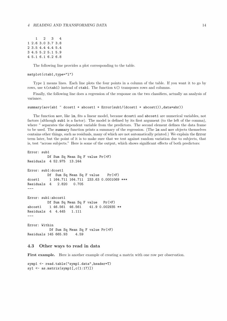
The following line provides a plot corresponding to the table.

matplot(ctab1,type="l")

Type l means lines. Each line plots the four points in a column of the table. If you want it to go byrows, use t(ctab1) instead of ctab1. The function t() transposes rows and columns.

Finally, the following line does a regression of the response on the two classifiers, actually an analysis ofvariance.

summary(aov(ab1 ~ dcost1 + abcost1 + Error(sub1/(dcost1 + abcost1)),data=abr))

The function aov, like lm, fits a linear model, because dcost1 and abcost1 are numerical variables, notfactors (although sub1 is a factor). The model is defined by its first argument (to the left of the comma),where ~ separates the dependent variable from the predictors. The second element defines the data frameto be used. The summary function prints a summary of the regression. (The lm and aov objects themselvescontains other things, such as residuals, many of which are not automatically printed.) We explain the Errorterm later, but the point of it is to make sure that we test against random variation due to subjects, thatis, test “across subjects.” Here is some of the output, which shows significant effects of both predictors:

Error: sub1Df Sum Sq Mean Sq F value Pr(>F)

Residuals 4 52.975 13.244

Error: sub1:dcost1Df Sum Sq Mean Sq F value Pr(>F)

dcost1 1 164.711 164.711 233.63 0.0001069 ***Residuals 4 2.820 0.705---

Error: sub1:abcost1Df Sum Sq Mean Sq F value Pr(>F)

abcost1 1 46.561 46.561 41.9 0.002935 **Residuals 4 4.445 1.111---

Error: WithinDf Sum Sq Mean Sq F value Pr(>F)

Residuals 145 665.93 4.59

4.3 Other ways to read in data

First example. Here is another example of creating a matrix with one row per observation.

symp1 <- read.table("symp1.data",header=T)sy1 <- as.matrix(symp1[,c(1:17)])


The first 17 columns of symp1 are of interest. The file symp1.data contains the names of the variablesin its first line. The header=T (an abbreviation for header=TRUE) makes sure that the names are used;otherwise the variables will be names V1, V2, etc.

gr1 <- factor(symp1$group1)

The variable group1, which is in the original data, is a factor that is unordered.

The next four lines create the new matrix, defining identifiers for subjects and items in a questionnaire.

syv1 <- as.vector(sy1)subj1 <- factor(rep(1:nrow(sy1),ncol(sy1)))item <- factor(rep(1:ncol(sy1),rep(nrow(sy1),ncol(sy1))))grp <- rep(gr1,ncol(sy1))cgrp <- ((grp==2) | (grp==3))+0

The variable cgrp is a code for being in grp 2 or 3. The reason for adding 0 is to make the logical vectorof T and F into a numeric vector of 1 and 0.

The following three lines create a table from the new matrix, plot the results, and report the results ofan analysis of variance.

sytab <- tapply(syv,list(item,grp),mean)matplot(sytab,type="l")svlm <- aov(syv ~ item + grp + item*grp)

Second example. In the next example, the data file has labels. We want to refer to the labels as if theywere variables we had defined, so we use the attach function.

t9 <- read.table("tax9.data",header=T)attach(t9)

Third example. In the next example, the data file has no labels, so we can read it with scan. The scanfunction just reads in the numbers and makes them into a vector, that is, a single column of numbers.

abh1 <- matrix(scan("abh1.data"),,224,byrow=T))

We then apply the matrix command to make it into a matrix. (There are many other ways to dothis.) We know that the matrix should have 224 columns, the number of variables, so we should specifythe number of columns. If you say help(matrix) you will see that the matrix command requires severalarguments, separated by commas. The first is the vector that is to be made into a matrix, which in this caseis scan("abh1.data"). We could have given this vector a name, and then used its name, but there is nopoint. The second and third arguments are the number of rows and the number of columns. We can leavethe number of rows blank. (That way, if we add or delete subjects, we don’t need to change anything.) Thenumber of columns is 224. By default, the matrix command fills the matrix by columns, so we need to saybyrow=TRUE or byrow=T to get it to fill by rows, which is what we want. (Otherwise, we could just leavethat field blank.)

We can refer to elements of abh1 by abh1[row,column]. For example, abh[1,2] is the sex of the firstsubject. We can leave one part blank and get all of it, e.g., abh1[,2] is a vector (column of numbers)representing the sex of all the subjects.


4.4 Other ways to transform variables

4.4.1 Contrasts

Suppose you have a matrix t1 with 4 columns. Each row is a subject. You want to contrast the mean ofcolumns 1 and 3 with the mean of columns 2 and 4. A t-test would be fine. (Otherwise, this is the equivalentof the cmatrix command in Systat.) Here are three ways to do it. The first way calculates the mean ofthe columns 1 and 3 and subtracts the mean of columns 2 and 4. The result is a vector. When we applyt.test() to a vector, it tests whether the mean of the values is different from 0.

t.test(apply(t1[c(1,3),],2,mean)-apply(t1[c(2,4),],2,mean))

The second way multiplies the matrix by a vector representing the contrast weights, 1, -1, 1, -1.Ordinary multiplication of a matrix by a vector multiplies the rows, but we want the columns, so we mustapply t() to transform the matrix, and then transform it back.

t.test(t(t(t1)*c(1,-1,1,-1)))

or

contr1 <- c(1,-1,1,-1)t.test(t(t(t1)*contr1))

The third way is the most elegant. It uses matrix multiplication to accomplish the same thing.

contr1 <- c(1,-1,1,-1)t.test(t1 %*% contr1)

4.4.2 Averaging items in a within-subject design

Suppose we have a matrix t2, with 32 columns. Each row is a subject. The 32 columns represent a 8x4design. The first 8 columns represent 8 different levels of the first variable, at the first level of the secondvariable. The next 8 columns are the second level of the second variable, etc. Suppose we want a matrix inwhich the columns represent the 8 different levels of the first variable, averaged across the second variable.

First method: loop. One way to do it — inelegantly but effectively — is with a loop. First, we set upthe resulting matrix. (We can’t put anything in it this way if it doesn’t exist yet.)

m2 <- t2[,c(1:8)]*0

The idea here is just to make sure that the matrix has the right number of rows, and all 0’s. Now hereis the loop:

for (i in 1:8) m2[,i] <- apply(t2[,i+c(8*0:3)],1,mean)

Here, the index i is stepped through the columns of m2, filling each one with the mean of four columnsof t2. For example, the first column of m2 is the mean of columns 1, 9, 17, and 25 of t2. This is because thevector c(8*0:3) is 0, 8, 16, 24. The apply function uses 1 as its second argument, which means to applythe function mean across rows.


Second method: matrix multiplication. Now here is a more elegant way, but one that requires anauxiliary matrix, which may use memory if that is a problem. This time we want the means according tothe second variable, which has four levels, so we want a matrix with four columns. We will multiply thematrix t2 by an auxiliary matrix c0.

The matrix c0 has 32 rows and four columns. The first column is 1,1,1,1,1,1,1,1 followed by 24 0’s. Thisis the result of rep(c(1,0,0,0),rep(8,4)), which repeats each of the elements of 1,0,0,0 eight times (sincerep(8,4) means 8,8,8,8). The second column is 8 0’s, 8 1’s, and 16 0’s.

c0 <- cbind(rep(c(1,0,0,0),rep(8,4)),rep(c(0,1,0,0),rep(8,4)),rep(c(0,0,1,0),rep(8,4)),rep(c(0,0,0,1),rep(8,4)))

c2 <- t2 %*% c0

The last line above uses matrix multiplication to create the matrix c2, which has 4 columns and one rowper subject. Note that the order here is important; switching t2 and c0 will not work.

4.4.3 Selecting cases or variables

There are several other ways for defining new matrices or data frames as subsets of other matrices or dataframes.

One very useful function is which(), which yields the indices for which its argument is true. For example,the output of which(3:10 > 4) is the vector 3 4 5 6 7 8, because the vector 3:10 has a length of 8, andthe first two places in it do not meet the criterion that their value is greater than 4. With which(), youcan use a vector to select rows or columns from a matrix (or data frame). For example, suppose you havenine variables in a matrix m9 and you want to select three sub-matrices, one consisting of variables 1, 4, 7,another with 2, 5, 8, and another with 3, 6, 9. Define mvec so that it is the vector 1 2 3 1 2 3 1 2 3.

mvec9 <- rep(1:3,3)m9a <- m9[,which(mvec9 == 1)]m9b <- m9[,which(mvec9 == 2)]m9c <- m9[,which(mvec9 == 3)]

You can use the same method to select subjects by any criterion, putting the which() expression beforethe comma rather than after it, so that it indicates rows.

4.4.4 Recoding and replacing data

Suppose you have m1 a matrix of data in which 99 represents missing data, and you want to replace each 99with NA. Simply say m1[m1==99] <- NA. Note that this will work only if m1 is a matrix (or vector), not adata frame (which could result from a read.table() command). You might need to use the as.matrix()function first.

Sometimes you want to recode a variable, e.g., a column in a matrix. If q1[,3] is a 7-point scale andyou want to reverse it, you can say

q1[,3] <- 8 - q1[,3]

In general, suppose you want to recode the numbers 1,2,3,4,5 so that they come out as 1,5,3,2,4, respec-tively. You have a matrix m1, containing just the numbers 1 through 5. You can say

c1 <- c(1,5,3,2,4)apply(m1,1:2,function(x) c1[x])


In this case c1[x] is just the value at the position indicated by x.

Suppose that, instead of 1 through 5, you have A through E, so that you cannot use numerical positions.You want to convert A,B,C,D,E to 1,5,3,2,4, respectively. You can use two vectors:

c1 <- c(1,5,3,2,4)n1 <- c("A","B","C","D","E")apply(m1,1:2,function(x) c1[which(n1)==x])

Or, alternatively, you can give names to c1 instead of using a second vector:

c1 <- c(1,5,3,2,4)names(c1) <- c("A","B","C","D","E")apply(m1,1:2,function(x) c1[x])

The same general idea will work for arrays, vectors, etc., instead of matrices.

Here are some other examples, which may be useful in simple cases, or as illustrations of various tricks.

In this example, q2[,c(2,4)] are two columns that must be recoded by switching 1 and 2 but leavingresponses of 3 or more intact. To do this, say

q2[,c(2,4)] <- (q2[,c(2,4)] < 3) * (3 - q2[,c(2,4)]) +(q2[,c(2,4)] >= 3) * q2[,c(2,4)]

Here the expression q2[,c(2,4)] < 3 is a two-column matrix full of TRUE and FALSE. By putting it inparentheses, you can multiply it by numbers, and TRUE and FALSE are treated as 1 and 0, respectively. Thus,(q2[,c(2,4)] < 3) * (3 - q2[,c(2,4)]) switches 1 and 2, for all entries less than 3. The expression(q2[,c(2,4)] >= 3) * q2[,c(2,4)] replaces all the other values, those greater than or equal to 3, withthemselves.

Here is an example that will switch 1 and 3, 2 and 4, but leave 5 unchanged, for columns 7 and 9

q3[,c(7,9)] <- (q3[,c(7,9)]==1)*3 + (q3[,c(7,9)]==2)*4 +(q3[,c(7,9)]==3)*1 + (q3[,c(7,9)]==4)*2 + (q3[,c(7,9)]==5)*5

Notice that this works because everything on the right of <- is computed on the values in q3 before any ofthese values are replaced.

4.4.5 Replacing characters with numbers

Sometimes you have questionnaire data in which the responses are represented as (for example) “y” and“n” (for yes and no). Suppose you want to convert these to numbers so that you can average them. Thefollowing command does this for a matrix q1, whose entries are y, n, or some other character for “unsure.”It converts y to 1 and n to -1, leaving 0 for the “unsure” category.

q1 <- (q1[,]=="y") - (q1[,]=="n")

In essence, this works by creating two new matrices and then subtracting one from the other, element byelement.

5 GRAPHICS 19

4.5 Using R to compute course grades

Here is an example that might be useful as well as instructive. Suppose you have a set of grades including amidterm with two parts m1 and m2, a final with two parts, and two assignments. You told the students thatyou would standardize the midterm scores, the final scores, and each of the assignment scores, then computea weighted sum to determine the grade. Here, with comments, is an R file that does this. The critical lineis the one that standardizes and computes a weighted sum, all in one command.

g1 <- read.csv("grades.csv",header=F) # get the list of scoresa1 <- as.vector(g1[,4])m1 <- as.vector(g1[,5])m2 <- as.vector(g1[,6])a2 <- as.vector(g1[,7])f1 <- as.vector(g1[,8])f2 <- as.vector(g1[,9])a1[a1=="NA"] <- 0 # missing assignment 1 gets a 0m <- 2*m1+m2 # compute midterm score from the partsf <- f1+f2gdf <- data.frame(a1,a2,m,f)gr <- apply(t(scale(gdf))*c(.10,.10,.30,.50),2,sum)# The last line standardizes the scores and computes their weighted sum# The weights are .10, .10, .30, and .50 for a1, a2, m, and f

gcut <- c(-2,-1.7,-1.4,-1.1,-.80,-.62,-.35,-.08,.16,.40,.72,1.1,2)# The last line defines cutoffs for letter grades.

glabels <- c("f","d","d+","c-","c","c+","b-","b","b+","a-","a","a+")gletter <- cut(gr,gcut,glabels) # creates a vector of letter gradesgrd <- cbind(g1[,1:2],round(gr,digits=4),gletter) # makes a matrix# gl[,1:2] are students’ names

grd[order(gr),] # sorts the matrix in rank order and prints itround(table(gletter)/.83,1) # prints, with rounding# the .83 is because there are 83 students, also gets percent

gcum <- as.vector(round(cumsum(table(gletter)/.83),1))names(gcum) <- glabelsgcum # prints cumulative sum of students with different grades

5 Graphics

R can do presentation-quality and publication-quality graphics. These often require some trial-and-errormanipulation of labels, line styles, axes, fonts, etc., and you should consult the help pages and the Introductionfor more details. The emphasis in this section is on the use of graphics for data exploration, but we providesome leads into the more advanced uses.

One trick with graphics is to know how each of the various graphics commands responds (or fails torespond) to each kind of data object: data.frame, matrix, and vector. Often, you can be surprised.

5.1 Default behavior of basic commands

Here is the default behavior for each object for each of some of the plotting commands, e.g., plot(x1) wherex1 is a vector, matrix, or data frame.

5 GRAPHICS 20

vector matrix data.frameplot values as function of position 2nd column as function of 1st plots of each column as func-

tion of othersboxplot one box for whole vector one box for all values in ma-

trixone box for each column(variable)

barplot one bar for each position,height is value

one bar for each column,summing successive values incolors

error

matplot one labeled point for each po-sition, height is value

X axis is row, Y is value, labelis column

X axis is row, Y is value, labelis column

The barplot of a matrix is an interesting display worth studying. Each bar is stack of smaller bars indifferent colors. Each smaller bar is a single entry in the matrix. The colors represent the row. Adjacentnegative and positive values are combined. (It is easier to understand this plot if all values have the samesign.)

5.2 Other graphics

To get a bar plot of the column means in a data frame df1, you need to saybarplot(height=apply(df1),2,mean)).

To get a nice parallel coordinate display like that in Systat, use matplot but transform the matrix anduse lines instead of points, that is: matplot(t(mat1),type="l"). You can abbreviate type with t.

matplot(v1, m1, type="l") also plots the columns of the matrix m1 on one graph, with v1 as thehorizontal axis. This is a good way to get plots of two functions on one graph.

To get scatterplots of the columns of a matrix against each other, use pairs(x1), where x1 is a matrixor data frame. (This is like “splom” in Systat, which is the default graph for correlation matrices.)

Suppose you have a measure y1 that takes several different values, and you want to plot histogramsof y1 for different values of x1, next to each other for easy comparison. The variable x1 has only two orthree values. A good plot is stripchart(y1 ~ x1, method=’stack’). When y1 is more continuous, trystripchart(y1 ~ x1, method=’jitter’).

Here are some other commands in their basic form. There are several others, and each of these has severalvariants. You need to consult the help pages for details.

plot(v1,v2) makes a scatterplot of v2 as a function of v1. If v1 and v2 take only a small number ofvalues, so that the plot has many points plotted on top of each other, try plot(jitter(v1),jitter(v2)).

hist(x1) gives a histogram of vector x1.

coplot(y1 ~ x1 | z1) makes several plots of y1 as a function of x1, each for a different range of valuesof z1.

interaction.plot(factor1,factor2,v1) shows how v1 depends on the interaction of the two factors.

Many wonderful graphics functions are available in the Grid and Lattice packages. Many of these areillustrated and explained in Venables and Ripley (1999).

5.3 Saving graphics

To save a graph as a png file, say png("file1.png"). Then run the command to draw the graph, such asplot(x1,y1). Then say dev.off(). You can change the width and height with arguments to the function.There are many other formats aside from png, such as pdf, and postscript. See help(Devices).

5 GRAPHICS 21

There are also some functions for saving graphics already made, which you can use after the graphic isplotted: dev.copy2eps("file1.eps") and dev2bitmap().

5.4 Multiple figures on one screen

The par() function sets graphics parameters. One type of parameter specifies the number and layout of multi-ple figures on a page or screen. This has two versions, mfrow and mfcol. The command par(mfrow=c(3,2)),sets the display for 3 rows and 2 columns, filled one row at a time. The command fpar(mfcol=c(3,2))also specifies 3 rows and 2 columns, but they are filled one column at a time as figures are plotted by othercommands.

Here is an example in which three histograms are printed one above the other, with the same horizontaland vertical axes and the same bar widths. The breaks are every 10 units. The freq=FALSE command meansthat densities are specified rather than frequencies. The ylim commands set the range of the vertical axis.The dev.print line prints the result to a file. The next three lines print out the histogram as numbersrather than a plot; this is accomplished with print=FALSE. These are then saved to hfile1.

par(mfrow=c(3,1))hist(vector1,breaks=10*1:10,freq=FALSE,ylim=c(0,.1))hist(vector2,breaks=10*1:10,freq=FALSE,ylim=c(0,.1))hist(vector3,breaks=10*1:10,freq=FALSE,ylim=c(0,.1))dev.print(png,file="file1.png",width=480,height=640)h1 <- hist(vector1,breaks=10*1:10,freq=FALSE,ylim=c(0,.1),plot=FALSE)h2 <- hist(vector2,breaks=10*1:10,freq=FALSE,ylim=c(0,.1),plot=FALSE)h3 <- hist(vector3,breaks=10*1:10,freq=FALSE,ylim=c(0,.1),plot=FALSE)sink("hfile1")h1h2h3sink()

For simple over-plotting, use par(new=T). Of course, this will also plot axis labels, etc. To avoid that,you might say par(new=T,ann=F). (Apparent undocumented feature: this setting conveniently disappearsafter it is used once.) To plot several graphs of the same type, you can also use points(), lines(), ormatplot().

5.5 Other graphics tricks

When you use plot() with course data (e.g., integers), it often happens that points fall on top of each other.There are at least three ways to deal with this. One is to use stripchart() (see above). Another is to applyjitter() to one or both of the vectors plotted against each other, e.g., plot(jitter(v1),v2). A third is touse sunflowerplot(v1,v2), which uses symbols that indicated how many points fall in the same location.

Use identify() to find the location and index of a point in a scatterplot made with plot(). Indicatethe point you want by clicking the mouse on it. The function locator() just gives the coordinates of thepoint. This is useful for figuring out where you want to add things to a plot, such as a legend.

text() uses a vector of strings instead of points in a plot. If you want a scatterplot with just thesename, first make an empty plot (with type="n") to get the size of the plot correct) and then use the textcommand, e.g.:

x <- 1:5

6 EXAMPLES OF SIMPLE GRAPHS IN PUBLICATIONS 22

plot(x,x^2,type="n")text(x,x^2,labels=c("one","two","three","four","five"),col=x)

In this case, the col=x argument plots each word in a different color.

To put a legend on a plot, you can use the “legend=” argument of the plotting function, or the legend()function, e.g., legend(3,4,legend=c("Self","Trust"),fill=c("gray25","gray75")). This example il-lustrates the use of gray colors indicated by number, which is convenient for making graphics for publication.(For presentation or data exploration, the default colors are usually excellent.)

Several functions will draw various things on graphs. polygon() and segments() draw lines. They differin the kind of input they want, and the first one closes the polygon it draws.

6 Examples of simple graphs in publications

This section illustrates some practical techniques for making publication-quality graphs with very basicgraphics commands.k

The second author, as editor of the open-access journal Judgment and Decision Making (http://journal.sjdm.org),has found it necessary to re-draw some graphs. Usually the originals were made with expensive proprietarysoftware, most of which is designed for printing on paper but sometimes is difficult to use for publicationgraphics, which usually must be re-sized to fit the journal’s format. For this purpose, the best format isencapsulated PostScript (eps).

But the eps format itself is not enough because of the two types of graphics formats. Vector graphicsdescribe images in terms of commands, of the form “draw a black line from point x1,y1 to point x2,y2.” Ofcourse, these commands are abbreviated in different ways for different formats. The details of which pointsshould be black are left to other software (or to a printer), which is usually designed to do the best possiblejob of displaying the element in question. On the other hand raster (or “bitmap”) images specify all thepoints. This works fine if the result is printed on paper or if the computer software plots the image point bypoint on the user’s display. If the image must be re-sized, however, the display program cannot fully recoverthe original information, and plots are usually somewhat messy. Common raster formats are tiff, png, gif,and bmp. Common vector formats are eps, svg (scalable vector graphics), wmf (Windows meta-file), and emf(extended wmf). But all of these “vector formats” can include raster images within them. Unfortunately,software that claims to produce eps often does it simply by making a raster image and including it in an epsfile. R is one of the few that makes true vector images correctly. (Others are Stata and SigmaPlot.)4

To produce good eps with R, I generally use the following format:

postscript(file="fig1.eps",width=8,height=8,horiz=F,onefile=F,pointsize=16,paper="special")[plotting commands here]dev.off()system("bbox fig1.eps")

All of these options are described in the help file for postscript() (in the graphics package), but somecomments are needed. First, pointsize controls the size of the font. A setting of 14 or 16 is good for a

4Note that the jpeg (or jpg) format, commonly used for photographs, is a third category. It is closer to a raster imageand is definitely not vector format. But it re-codes the images into a more compact format by using interesting mathematicaltransformations (involving singular value decomposition), which preserve the useful information found in most photographs.It is called a “lossy” format because it loses some information. It should not be used for “line art,” that is, graphs, but itis practically necessary for photos. Although most digital cameras now have a tiff (raster) option, it is rarely used because itrequires much more storage space than jpeg.


large figure that covers the width of a page, but usually 18 or 20 is better for a figure that will go in a singlecolumn of a two-column text. Note that the advantage of eps is that you can resize it, without loss, to fitwherever it goes.

The dev.off() command is necessary to save the result to disk.

For all the niceties of R , there is one thing it doesn’t do, which is to make a “tight bounding box” arounda plot. The difference between eps and ordinary Postscript is the specification of a bounding box, which is adescription of the box containing the plot. You can see these commands by looking at the top of almost anyeps file, which is just text. The problem is that R ’s default bounding box includes a blank margin, whichyou usually do not want. To remove the margin, I use the following script (which requires Ghostscript anduses Linux shell commands, which can probably be translated for other operating systems):

#!/bin/bashcat $1 | sed -r -e "s/BoundingBox:[\ ]+[0-9]+[\ ]+[0-9]+[\ ]+[0-9]+[\ ]+\[0-9]+/‘gs -sDEVICE=bbox -dBATCH -dNOPAUSE -q‘/" > temp.eps

gs -sDEVICE=bbox -sNOPAUSE -q $1 $showpage -c quit 2> bb.outsed -e"1 r bb.out" temp.eps > $1/bin/rm bb.out/bin/rm temp.eps

Note that the first line of this script is folded to make it easier to read here. It should be unfolded. Thisscript removes the original bounding box and replaces it with the smallest possible box. The system()command above simply calls the script.

Each of the following examples is listed according to the URL of the paper in which it appears. Thecomplete R scripts for these and other figures are linked from http://journal.sjdm.org/RX.html

6.1 http://journal.sjdm.org/8827/jdm8827.pdf

500

550

600

650

700

Distance from target

Mea

n R

T (

mill

isec

on

ds)

Near Far

683

605

648

594

619

577

520

489

525

507

First quintile: Largest distance−effect slope

Second quintileThird quintile

Fourth quintile

Fifth quintile: Smallest distance−effect slope


postscript(file="fig1.eps",width=8,height=8,horiz=F,onefile=F,pointsize=16,paper="special")c1 <- c(683,605)c2 <- c(648,594)c3 <- c(619,577)c4 <- c(520,489)c5 <- c(525,507)plot(c1,xlab=expression(bold("Distance from target")),

ylab=expression(bold("Mean RT (milliseconds)")),ylim=c(475,700),xlim=c(.8,2.2),type="b",xaxt="n")

axis(1,at=c(1,2),labels=c("Near","Far"))lines(c2,type="b")lines(c3,type="b")lines(c4,type="b")lines(c5,type="b")text(c(.92,2.08),c1,labels=c1)text(c(.92,2.08),c2,labels=c2)text(c(.92,2.08),c3,labels=c3)text(c(.92,2.08),c4,labels=c4)text(c(.92,2.08),c5,labels=c5)text(1.5,mean(c1)+8.6,srt=-23,labels="First quintile: Largest distance-effect slope")text(1.5,mean(c2)+7,srt=-16,labels="Second quintile")text(1.5,mean(c3)+7,srt=-12,labels="Third quintile")text(1.5,mean(c4)-7.4,srt=-9.2,labels="Fourth quintile")text(1.5,mean(c5)+8.8,srt=-5.4,labels="Fifth quintile: Smallest distance-effect slope")dev.off()system("bbox fig1.eps")

This figure illustrates the use of the text() function. Here I adjusted the slope with srt by trial anderror, although the initial errors got smaller after the first one.


−2

−1

01

23

4

Pre

dict

ed p

refe

renc

e

1st quintileLargest

distance−effectslope

2nd quintile 3rd quintile 4th quintile 5th quintileSmallestdistance−

effectslope

Distance−effect slope quintile split

0.9

2.0

2.6

3.3

4.0

−1.6−1.3

−1.1 −1.0−0.8

$10/$15 choice

$100/$110 choice

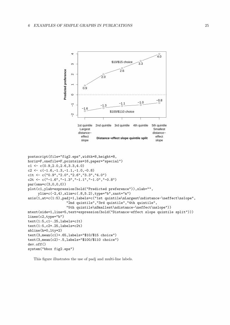
postscript(file="fig2.eps",width=8,height=8,horiz=F,onefile=F,pointsize=16,paper="special")c1 <- c(0.9,2.0,2.6,3.3,4.0)c2 <- c(-1.6,-1.3,-1.1,-1.0,-0.8)c1t <- c("0.9","2.0","2.6","3.3","4.0")c2t <- c("-1.6","-1.3","-1.1","-1.0","-0.8")par(oma=c(3,0,0,0))plot(c1,ylab=expression(bold("Predicted preference")),xlab="",

ylim=c(-2,4),xlim=c(.8,5.2),type="b",xaxt="n")axis(1,at=c(1:5),padj=1,labels=c("1st quintile\nLargest\ndistance-\neffect\nslope",

"2nd quintile","3rd quintile","4th quintile","5th quintile\nSmallest\ndistance-\neffect\nslope"))

mtext(side=1,line=5,text=expression(bold("Distance-effect slope quintile split")))lines(c2,type="b")text(1:5,c1-.25,labels=c1t)text(1:5,c2+.25,labels=c2t)abline(h=0,lty=2)text(3,mean(c1)+.65,labels="$10/$15 choice")text(3,mean(c2)-.5,labels="$100/$110 choice")dev.off()system("bbox fig2.eps")

This figure illustrates the use of padj and multi-line labels.



5.0

5.5

6.0

6.5

7.0

7.5

8.0

8.5

Number of arguments

Beh

avio

ral i

nten

tion

2 4 6 | 2 4 6 | 2 4 6

Positivebackground

Negativebackground

Nobackground

Frame:

GainLoss

Intent <- array(c(7.32,7.60,7.80,5.28,7.44,8.24,7.96,7.40,8.08,7.50,6.76,7.48,7.52,7.28,6.48,6.80,7.72,7.48),c(3,3,2))dimnames(Intent) <- list(Arguments=c(2,4,6),

Background=c("Positive","Negative","None"),Frame=c("Positive","Negative"))

Intention <- c(Intent)Arguments <- rep(c(2,4,6),6)Background <- rep(rep(c("Positive","Negative","None"),c(3,3,3)),2)Frame <- rep(c("Positive","Negative"),c(9,9))

postscript(file="fig0.eps",width=8,height=8,horiz=F,onefile=F,pointsize=18,paper="special")

plot(c(2,4,6),Intention[1:3],xlim=c(2,18),ylim=c(5,8.5),pch=19,col="maroon",xlab="Number of arguments",ylab="Behavioral intention",xaxt="n")

y.lm <- fitted(lm(Intention[1:3] ~ c(2,4,6)))segments(2, y.lm[1], 6, y.lm[3],col="maroon")points(c(8,10,12),Intention[4:6],col="maroon",pch=19)y.lm <- fitted(lm(Intention[4:6] ~ c(8,10,12)))segments(8, y.lm[1], 12, y.lm[3],col="maroon")points(c(14,16,18),Intention[7:9],col="maroon",pch=19)y.lm <- fitted(lm(Intention[7:9] ~ c(14,16,18)))segments(14, y.lm[1], 18, y.lm[3],col="maroon")

points(c(2,4,6),Intention[10:12],col="blue")y.lm <- fitted(lm(Intention[10:12] ~ c(2,4,6)))segments(2, y.lm[1], 6, y.lm[3],col="blue",lty=2)


points(c(8,10,12),Intention[13:15],col="blue")y.lm <- fitted(lm(Intention[13:15] ~ c(8,10,12)))segments(8, y.lm[1], 12, y.lm[3],col="blue",lty=2)points(c(14,16,18),Intention[16:18],col="blue")y.lm <- fitted(lm(Intention[16:18] ~ c(14,16,18)))segments(14, y.lm[1], 18, y.lm[3],col="blue",lty=2)

mtext(side=1,line=1,at=c(1,2,3,3.5,4,5,6,6.5,7,8,9)*2,text=c(2,4,6,"|",2,4,6,"|",2,4,6))

abline(v=7)abline(v=13)text(c(4,10,16),5.15,labels=c("Positive\nbackground",

"Negative\nbackground","No\nbackground"))legend(14,6.42,legend=c("Gain","Loss"),title="Frame:",

col=c("maroon","blue"),pch=c(19,1))dev.off()system("bbox fig0.eps")

This is a fairly complicated example, which illustrates several things. One is the use of lm() to getproperties of best-fitting lines to superimpose on a plot. In simple cases, it is usually sufficient to saysomething like abline(lm(Y X)). But here the origin is different for each part of the plot, so we use fittedvalues and segments() instead of abline(). Also shown here is the use of mtext() to add text around themargins of a plot, just as text() adds test internally. Finally, we use legend() to specify more carefullywhere the legend should go.


Pre

dict

ion

accu

racy

Total Mouselab Eyetracking

Consistenttrials

Inconsistenttrials

Choicetrials

Deferraltrials

0%25

%50

%75

%10

0%

66% 69% 63% 78% 40% 70% 53%

n.s.

}

library(gplots)

c1 <- c(66,69,63,78,40,70,53)e1 <- c(3,4,4,4,3,4,8)postscript(file="fig4.eps",width=10.8,height=8,horiz=F,onefile=F,pointsize=16,paper="special")


barplot2(height=c1,plot.ci=T,ci.u=c1+e1,ci.l=c1-e1,xaxt="n",yaxt="n",ylab="Prediction accuracy",ylim=c(0,100),width=c(.5,.5),space=1)

axis(1,at=(1:7)-.25,padj=.5,lty=0,labels=c("Total\n","Mouselab\n","Eye\ntracking","Consistent\ntrials",

"Inconsistent\ntrials","Choice\ntrials","Deferral\ntrials"))axis(2,at=c(0,25,50,75,100),labels=c("0%","25%","50%","75%","100%"))text((1:7)-.25,10,labels=paste(c1,"%",sep=""))text(3.15,72,labels="n.s.")text(3.15,65.6,labels="}",cex=1.75,lwd=.1)dev.off()system("bbox fig4.eps")

For adding confidence intervals, the easiest way is to use the gplots package, as illustraged here. Thisplot also illustrates the use of axis(), and the use of cex to make a large character, in this case a bracket.The lwd option is necessary to keep the bracket from being too thick. Trial and error are needed.


r(t)

= v

alu

e(L

eft −

Rig

ht)

r(t) = r(t − 1) + f(vtarget, vnon−target) + ut

barrier right

barrier left choose left

left right left

time

postscript(file="fig1.eps",family="NimbusSan",width=8,height=8,horiz=F,onefile=F,pointsize=16,paper="special")plot(0:100,0:100,type="n",axes=F,,xlab="",ylab="")rect(0,30,20,70,col="#EEEEFF",border=NA)rect(20,30,45,70,col="#FFFFDD",border=NA)rect(45,30,95,70,col="#EEEEFF",border=NA)lines(c(0,0),c(25,75))lines(c(0,100),c(30,30),col="red",lty=2)lines(c(0,100),c(70,70),col="red",lty=2)lines(c(0,100),c(50,50))segments(x0=c(0,20,45),y0=c(50,60,45),x1=c(20,45,95),y1=c(60,45,70),lwd=2)points(95,70,cex=4)mtext("r(t) = value(Left - Right)",side=2)text(4,65,expression(r(t) == r(t-1) + f(v[target],v[non-target]) + u[t]), pos=4)text(10,25,"barrier right",pos=4,col="red")text(10,75,"barrier left",pos=4,col="red")text(95,77,"choose left")text(c(0,20,45,85),c(33,33,33,47),labels=c("left","right","left","time"),pos=4)lines(c(20,20),c(30,70),lty=3)lines(c(45,45),c(30,70),lty=3)dev.off()


system("bbox fig1.eps")

This plot illustrates the inclusion of a mathematical expression as text, as well as the use of rect tomake shaded rectangles.


fixation cue appears

saccad targets appear

go cue presented

saccade executed

reward deliveredtime

Ch=14postscript(file="fig1.eps",family="NimbusSan",width=8,height=8,horiz=F,onefile=F,pointsize=16,paper="special")plot(c(0,110),c(0,100),type="n",axes=F,xlab="",ylab="")rect(0,80,20,100,col="gray80")rect(0+Ch,80-Ch,20+Ch,100-Ch,col="gray80")rect(0+2*Ch,80-2*Ch,20+2*Ch,100-2*Ch,col="gray80")rect(0+3*Ch,80-3*Ch,20+3*Ch,100-3*Ch,col="gray80")rect(0+4*Ch,80-4*Ch,20+4*Ch,100-4*Ch,col="gray80")text(20,98,pos=4,labels="fixation cue appears")text(20+Ch,98-Ch,pos=4,labels="saccad targets appear")text(20+2*Ch,98-2*Ch,pos=4,labels="go cue presented")text(20+3*Ch,98-3*Ch,pos=4,labels="saccade executed")text(20+4*Ch,98-4*Ch,pos=4,labels="reward delivered")points(c(10, 10+Ch,10+Ch-6,10+Ch+6, 10+2*Ch-6,10+2*Ch+6, 10+3*Ch-6),

c(90, 90-Ch,90-Ch-6,90-Ch+6, 90-2*Ch-6,90-2*Ch+6, 90-3*Ch-6),pch=20)

arrows(0,70,3.5*Ch,70-3.5*Ch,lwd=2)text(25,80-3*Ch,labels="time")arrows(10+3*Ch,90-3*Ch,10+3*Ch-5,90-3*Ch-5,length=0.1)par(new=TRUE)xspline(87+c(0,2,0,-2),33+c(4,0,-2,0),open=F,shape=c(0,1,1,1))dev.off()system("bbox fig1.eps")

This shows how rectangles can overlap. The droplet of sweetened water in the last rectangle was a bit of


a problem because no character seemed to have the shape of a droplet. Thus, we used xspline() to draw itpiece by piece (with much trial and error). Another feature is the setting of the constant Ch, which helpedget the dimensions right.


0.0 0.2 0.4 0.6 0.8 1.0

0.0

0.2

0.4

0.6

0.8

1.0

Expected probability

Ob

se

rved p

rob

ab

ility

P <- c(0.0000616649,0.0012931876,0.0014858932,0.0034575074,0.0095432743,0.0112784208,0.0198140078,0.0260565422,0.0378525090,0.0476971273,0.0665802025,0.1160787054,0.1561110462,0.1741858728,0.2592136466,0.3849843314,0.3970805883,0.4387950690,0.5686058809,0.5880746208,0.6367807765,0.7164637107,0.7548314071,0.8594174096,0.8637551603,0.8852179374,0.8854362373,0.8904200780,0.9319782385,0.9411071229,0.9474470330,0.9605232158,0.9621474910,0.9716238220,0.9750371388,0.9800862502,0.9856935080,0.9923052342,0.9993104279,0.9994746329,0.9997647547,0.9999417310,0.9999506389,0.9999650462,0.9999825779,0.9999967088,0.9999994243,0.9999999681)

ordinate <- sort(P)n <- length(ordinate)plotpos <- seq(0.5/n, (n - 0.5)/n, by = 1/n)postscript(file="fig1.eps",family="NimbusSan",width=8,height=8,horiz=F,onefile=F,pointsize=16,paper="special") # was 20, changed for sinica paperplot(ordinate, plotpos, xlab="Expected probability",

ylab="Observed probability")abline(0,1,lty=3)grid()dev.off()system("bbox fig1.eps")

7 STATISTICS 31

This example is of substantive interest. It shows the p-values for a set of t-tests, one for each subject. Theabscissa is the percentile rank of the p-value. If the data were random, the plot would be on the diagonal.The 5th percentile would have p = .05, because 5% of the p-values would be significant at the .05 level. Asis apparent, the curve departs from the expectation at both ends, showing that subjects show significanteffects in both directions. This example is discussed in Baron (in press).

6.7 Boxes and arrows

This figure illustrates the use of William Revelle’s psych package for making boxes and arrows. (This plotwas for an article but was omitted in the final version.) It also illustrates how to include Greek letters.

Vividnessmanipulation

Anticipatedregret

Exchangetickets

β = 1.00

4, p

< .0

05 χ 2= 6.2, p < .05

χ2 = 3.07

library(psych)xlim=c(0,6)ylim=c(0,4)plot(NA,xlim=xlim,ylim=ylim,axes=FALSE,xlab="",ylab="")r1 <- dia.rect(1,1,"Vividness\nmanipulation",xlim=xlim,ylim=ylim)r2 <- dia.rect(3,2.3,"Anticipated\nregret",xlim=xlim,ylim=ylim)r3 <- dia.rect(5,1,"Exchange\ntickets",xlim=xlim,ylim=ylim)dia.arrow(from=r1$top,to=r2$left)dia.arrow(from=r1,to=r3)dia.arrow(from=r2$right,to=r3$top)text(1.6,1.85,labels=expression(paste(beta == 1.004,", p < .005")),srt=46)text(4.4,1.85,labels=expression(paste(chi^2 == 6.2,", p < .05")),srt=-46)text(3,1.2,labels=expression(chi^2 == 3.07))

dev.copy2eps(file="fig1.eps")dev.off()system("bbox fig1.eps")

7 Statistics

This section is not a summary of all statistics but, rather, a set of notes on procedures that are more usefulto the kind of studies that psychology researchers do.

7.1 Very basic statistics

Here is a list of some of the commands psychologists use all the time:

7 STATISTICS 32

t.test(a1,b1) — Test the difference between the means of vectors a1 and b1.

t.test(a1,b1,paired=TRUE) or t.test(a1,b1,p=T), or, even simpler, t.test(b1-a1) — Test the dif-ference between means of vectors a1 and b1 when these represent paired measures, e.g., variables for thesame subject. The vectors can be parts of matrices or data.frames. A good plot to look at is

plot(a1,b1)abline(0,1)

This plots b1 as a function of a1 and then draws a diagonal line with an intercept of 0 and a slope of 1.Another plot is matplot(t(cbind(a1,b1)),type="l"), which shows one line for each pair.

Sometimes you want to do a t-test comparing two groups represented in the same vector, such as malesand females. For example, you have a vector called age1 and a vector called sex1, both of the samelength. Subject i1’s age and sex are age1[i1] and sex1[i1]. Then a test to see if the sexes differ in age ist.test(age1[sex1==0],age1[sex1==1]) (or perhaps t.test(age1[sex1==0],age1[sex1==1],var.equal=T)for the assumption of equal variance). A good plot to do with this sort of test isstripchart(age1 sex1,method=’jitter’) (or stripchart(age1 sex1,method=’stack’) if there are onlya few ages represented).

The binomial test (sign test) for asking whether heads are more likely than tails (for example) usesprop.test(h1,n1), where h1 is the number of heads and n1 is the number of coin tosses. Suppose you havetwo vectors a1 and b1 of the same length, representing pair of observations on the same subjects, and you wantto find whether a1 is higher than b1 more often than the reverse. Then you can say prop.test(sum(a1>b1),sum(a1>b1)+sum(a1<b1)). The use of the sum of sums as the second argument excludes those cases wherea1==b1. prop.test can also be used to compare several different proportions. (See the help file.)

chisq.test(x1) does a chi-square test on a matrix x1, where the cells represent counts in a classificationtable. There are several other ways of using this function. One other useful one is chisq.test(a1,b1),where a1 and b1 are vectors or factors of the same length, representing the levels on which observations areclassified. For example,

a1 <- c(1,1,1,1,1,1,1,0,0,0,0,0,0)b1 <- c(1,1,1,1,1,1,0,0,0,0,0,0,1)chisq.test(a1,b1)

will yield an almost significant result, since the two vectors match except for two cases. If you want a Fisherexact test instead of chi-square (for a 2x2 table), you just use fisher.test() instead of chisq.test().

A related test is mantelhaen.test. It, and many useful nonparametric tests, are in the ctest package(which is loaded automatically but has its own help listing separate from base). Some of these tests can beexact. More generally, see the loglin function, which requires no special package, and the loglm functionin the MASS package, which allows models to be specified in a form like linear models.

cor(a1) — Show the correlations of the columns for a matrix or data frame a1.

cor.test(a1,b1) — Show the correlation between vectors a1 and b1 and its significance.

Partial correlation is the correlation of the residuals, and this is one way to compute it. Thus, the partialcorrelation of x1 and y1, partialling z1, is cor(lm(x1~z1)$resid,lm(y1~z1)$resid). As we shall explain,lm is the function to fit a linear model, and resid is one of the elements that it returns (not usually printed,but available). The significance of the partial correlation is the same as the significance of the regressioncoefficient, so (again, as we shall explain) use summary(lm(x1 ~ y1 + z1)) to get it.

For factor analysis, you need the mva library, so say library(mva) to load it. The main command isfactanal(m1,factors=3). (The number of factors can be varied.) Varimax is the default rotation, but youcan also say, for example, factanal(m1,factors=4,rotation="promax").

7 STATISTICS 33

Principal components analysis is also in the mva library. The most useful commands are print(prcomp(x1))to get the components of matrix or data.frame x1, and plot(prcomp(x1)) to see a scree plot of the variancesaccounted for by the components. The eigenvalues are the squares of the sdev values that are part of theoutput of print(prcomp(x1)).

The same library also does cluster analysis, e.g., kmeans(x1,3) where 3 is the number of clusters. If youwant to define a factor identifying the cluster of each subject, you can sayf1 <- as.factor(kmeans(x1,3)$cluster), or, if you just want the numbers and don’t care about whetheryou have a factor, v1 <- kmeans(x1,3)$cluster. To see a plot of the variable means for the 3 clusters, saymatplot(t(v1),t="l"). (The last part abbreviates type="lines".

Multiple tests are well handled by the multtest package, with is part of the Bioconductor packages. (SeeSection 2.2.2.) The documentation in that package provides a good introduction, with citations. The classicBonferroni method is often unnecessarily conservative. On the other hand, multiple tests can sometimes beavoided by clear statement of a hypothesis and an effort to find the single best test of it.

7.2 Reliability of a test

Suppose v1 is a matrix in which the rows are subjects and each column is a test item. You want to calculatethe coefficient alpha, a measure of the reliability of the test (Lord & Novick, 1968, p. 88):

α =n

n− 1

[1−

∑σ2(Yi)σ2

X

]

Here is the expression of this in R. (Alpha is now available in the psy package.) The expression nv is thenumber of variables. (If you know this, you can just put it in the formula instead of nv).

nv1 <- ncol(v1)(nv1/(nv1-1))*(1 - sum(apply(v1,2,var))/var(apply(v1,1,sum)))

Crucial here is the use of the apply function to rows and columns. The first use of apply finds thevariance of each column of the matrix. The 2 indicates columns. Then we take the sum of these. The secondapplication finds the total score for each subject by applying the function sum to each row. We then find thevariance of this sum.

Another way to compute alpha involves the variance-covariance matrix of the items.

tvar1 <- var(v1, na.rm = FALSE) # missing data aborts var()

The sum of values along the main diagonal of the variance-covariance matrix (tvar1) equals the numeratorof the right-hand term in the formula, and the sum of all elements in tvar1 equals the denominator, so alphais:

(nv1/(nv1-1)) * (1 - sum(diag(tvar1))/sum(tvar1))

This approach is better for large data sets, because the apply function uses a lot of memory.

Now suppose that you want to see what happens if you delete item 3. You can do this by deletingvariables in each formula (remembering in each case to change the value of nv1):

(nv1/(nv1-1)*(1 - sum(apply(v1[,-3],2,var))/var(apply(v1[-3],1,sum)))

(nv1/(nv1-2)) * (1 - sum(diag(tvar[-3,-3]))/sum(tvar[-3,-3]))

7 STATISTICS 34

The advantage of using the variance-covariance matrix is that the effect of deleting certain items can bedetermined easily.

7.3 Goodman-Kruskal gamma

The Goodman-Kruskal gamma statistic (also known as γ) is like tau (τ) except for the denominator. It isan easily interpreted measure of rank correlation between two vectors v1 and v2. The idea is to consider allpairs of observations in each vector: observations 1 and 2, 1 and 3, and so on. Count the number of timestheir ordering agrees, and call this S+. Count the number of times their ordering disagrees and call this S-.If one variable is tied, this does not count either way. Then γ = S+−S−

S++S− . In other words, it is the number ofagreements minus the number of disagreements, all divided by the total of agreements and disagreements.A γ of 1 means that the correlation is as high as it can be, given the ties.

Gamma is available in the Hmisc package, in the rcorr.cens() function. To compute it for v1 and v1,say rcorr.cens(v1,v2,outx=T). The outx argument concerns whether ties are ignored (as they should be).The Dxy value is what you want.

An instructive, but slower, function to compute gamma is:

goodman <- function(x,y){Rx <- outer(x,x,function(u,v) sign(u-v))Ry <- outer(y,y,function(u,v) sign(u-v))S1 <- Rx*Ryreturn(sum(S1)/sum(abs(S1)))}

To compute gamma for v1 and v2, say goodman(v1,v2).

7.4 Inter-rater agreement

An interesting statistical question came up when we started thinking about measuring the agreement betweentwo people coding video-tapped interviews. This section discusses two such measures. One is the percentageagreement among the raters, the other is the kappa statistic commonly used for assessing inter-rater reliability(not to be confused with the R function called kappa). We will first summarize how either of them is derived,then we will use an example to show that kappa is better than percentage agreement. (Kappa is now availablein the concord package, and another version in psy for more than two raters.)

Our rating task is as follows. Two raters, LN and GF, viewed the video-tapped interviews of 10 families.The raters judged the interviews on a check list of 8 items. The items were about the parent’s attitude andgoals. The rater marks a ’yes’ on an item if the parents expressed feelings or attitudes that fit the item and’no’ otherwise. A yes is coded as 1 and a no 0.

The next table shows how the two raters classified the 10 families on Items 2 and 4.Family

Item 2A B C D E F G H I J

LN 0 0 0 0 1 1 1 1 1 1GF 0 1 1 1 1 1 1 1 1 1

Item 4LN 0 1 0 0 1 1 0 0 0 0GF 0 1 0 0 1 0 0 1 0 1

Note that in both items, the two raters agreed on the classifications of 7 out of 10 families. However, InItem 4, rater LN gave more no’s and GF gave about equal yeses and no’s. In Item 2, rater GF gave 9 yeses

7 STATISTICS 35

and only 1 no. It turns out that this tendency to say yes or no affects the raters’ agreement adjusted forchance. We will get to that in a moment.

Suppose that Item 2 was whether or not our interviewees thought that “learning sign language willmitigate the development of speech for a child who is deaf or hard of hearing”. We want to know how muchLN and GF agreed. The agreement is what we call an inter-rater reliability. They might agree positively(both LN and GF agreed that the parents thought so) or negatively (i.e., a no - no pair).

Our first measure, the percentage of agreement, is the proportion of families that the raters made thesame classifications. We get a perfect agreement (100%) if the two raters make the same classification forevery family. A zero percent means complete disagreement. This is straightforward and intuitive. Peopleare familiar with a 0% to 100% scale.

One problem with percent agreement is that it does not adjust for chance agreement, the chance thatthe raters happen to agree on a particular family. Suppose, for example, that after the raters have forgottenwhat they did the first time, we ask them to view the videotape of family A again. Pure chance may leadto a disagreement this time; or perhaps even an agreement in the opposite direction.

That is where the κ statistic comes in. Statistics like kappa adjust for chance agreement by subtractingthem out:

κ =Pr(observed agreement)− Pr(chance agreement)

Pr(maximum possible agreement)− Pr(chance agreement),

where the chance agreement depends on the marginal classifications. The marginal classifications, in ourcase, refer to each rater’s propensity to say “yes” or “no”. The chance agreement depends in part on howextreme the raters are. If, for example, rater 1 gave 6 yeses and 4 no’s and rater 2 gave 9 yeses and only 1no, then there is a higher chance for the raters to agree on yes-yes rather than no-no; and a disagreement ismore likely to occur when rater 2 says yes and rater 1 says no.

Therefore, for the same proportion of agreement, the chance-adjusted kappa may be different. Althoughwe do not usually expect a lot of difference. We can use the following example to understand how it works.

The numbers in the following table are the number of families who were classified by the raters. In bothitems, raters LN and GF agreed on the classification of 7 families and disagreed on 3 families. Note thatthey had very different marginal classifications.

If we only look at the percentage of agreement, then LN and GF have the same 70% agreement on Items2 and 4. However, the κ agreement is 0.29 for Item 2 and 0.35 for Item 4.

Item 2 Item 4rater GF rater GF

yes no marginal yes no marginalrater yes 6 0 6 2 1 3LN no 3 1 4 2 5 7

9 1 10 4 6 10

Why? We can follow the formula to find out. In both items, the observed agreement, when expressed ascounts, is the sum of the numbers along the diagonal. For Item 2 it is (6 + 1) = 7. Divide that by 10 youget 70% agreement. The maximum possible number of agreement is therefore 10/10.

The chance agreement for Item 2 is (6/10) × (9/10) + (4/10) × (1/10). That is the probability of bothraters said ‘yes’ plus both said ‘no’. Rater LN gave 6 yeses and GF gave 9 yeses. There is a 6

10 probabilityfor LN to say yes and a 9

10 probability for GF to say yes. Therefore, the joint probability, i.e., the chancefor us to get a yes-yes classification, is 6

10 × 910 . Similarly, the probability of a no-no classification is 4

10 × 110 .

For Item 2, we have κ = 710 − 58

100/ 1010 − 58

100 = 0.29. The κ for Item 4 is 710 − 54

100/1010 − 54

100 = 0.35. Thekappa statistics are different between Items 2 and 4 because their chance agreements are different. One is 58

100and the other is 54

100 . The marginals of the two tables show us that the two raters made more yes judgmentsin one instance and more no judgments in the other. That in itself is OK, the raters make the classifications

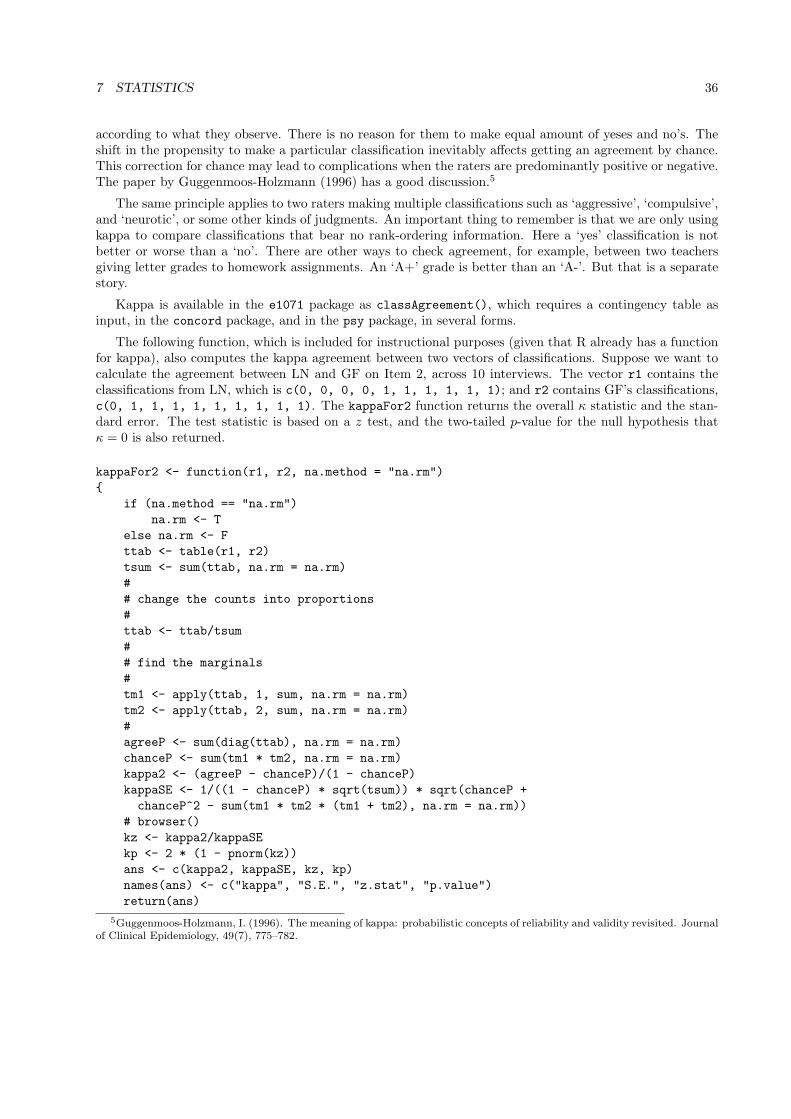
7 STATISTICS 36

according to what they observe. There is no reason for them to make equal amount of yeses and no’s. Theshift in the propensity to make a particular classification inevitably affects getting an agreement by chance.This correction for chance may lead to complications when the raters are predominantly positive or negative.The paper by Guggenmoos-Holzmann (1996) has a good discussion.5

The same principle applies to two raters making multiple classifications such as ‘aggressive’, ‘compulsive’,and ‘neurotic’, or some other kinds of judgments. An important thing to remember is that we are only usingkappa to compare classifications that bear no rank-ordering information. Here a ‘yes’ classification is notbetter or worse than a ‘no’. There are other ways to check agreement, for example, between two teachersgiving letter grades to homework assignments. An ‘A+’ grade is better than an ‘A-’. But that is a separatestory.

Kappa is available in the e1071 package as classAgreement(), which requires a contingency table asinput, in the concord package, and in the psy package, in several forms.

The following function, which is included for instructional purposes (given that R already has a functionfor kappa), also computes the kappa agreement between two vectors of classifications. Suppose we want tocalculate the agreement between LN and GF on Item 2, across 10 interviews. The vector r1 contains theclassifications from LN, which is c(0, 0, 0, 0, 1, 1, 1, 1, 1, 1); and r2 contains GF’s classifications,c(0, 1, 1, 1, 1, 1, 1, 1, 1, 1). The kappaFor2 function returns the overall κ statistic and the stan-dard error. The test statistic is based on a z test, and the two-tailed p-value for the null hypothesis thatκ = 0 is also returned.

kappaFor2 <- function(r1, r2, na.method = "na.rm"){

if (na.method == "na.rm")na.rm <- T

else na.rm <- Fttab <- table(r1, r2)tsum <- sum(ttab, na.rm = na.rm)## change the counts into proportions#ttab <- ttab/tsum## find the marginals#tm1 <- apply(ttab, 1, sum, na.rm = na.rm)tm2 <- apply(ttab, 2, sum, na.rm = na.rm)#agreeP <- sum(diag(ttab), na.rm = na.rm)chanceP <- sum(tm1 * tm2, na.rm = na.rm)kappa2 <- (agreeP - chanceP)/(1 - chanceP)kappaSE <- 1/((1 - chanceP) * sqrt(tsum)) * sqrt(chanceP +chanceP^2 - sum(tm1 * tm2 * (tm1 + tm2), na.rm = na.rm))

# browser()kz <- kappa2/kappaSEkp <- 2 * (1 - pnorm(kz))ans <- c(kappa2, kappaSE, kz, kp)names(ans) <- c("kappa", "S.E.", "z.stat", "p.value")return(ans)

5Guggenmoos-Holzmann, I. (1996). The meaning of kappa: probabilistic concepts of reliability and validity revisited. Journalof Clinical Epidemiology, 49(7), 775–782.

7 STATISTICS 37

}

Sometimes a function requires further editing. Suppose the kappaFor2 function is entered at R’s systemprompt (i.e., the > character), and there was an error. Then we can type the command kappaFor2 <- emacs(kappaFor2)to edit its contents with the emacs editor; or use vi() for the visual editor. In the above function thereis a browser() command, commented out by a # character. The browser() command is used to debuga function. Each time R runs the kappaFor2 function, it stops at the point where a working browser()command was set, and we can debug the function by examining the variables inside the function.

We run the function kappaFor2 and the results show that the agreement on Item 2 is not reliably greaterthan 0, with a two-tail p-value of about 0.20.

> kappaFor2(r1 = c(0, 0, 0, 0, 1, 1, 1, 1, 1, 1),r2 = c(0, 1, 1, 1, 1, 1, 1, 1, 1, 1))

kappa S.E. z.stat p.value0.2857143 0.2213133 1.2909944 0.1967056

7.5 Generating random data for testing

Suppose you want to test that the last two formulas yield the same result, but you don’t have any datahandy. You can generate a sample of 10 Likert-type, 5-point scale responses from 100 Ss as follows:

v1 <- matrix(sample(c(1, 2, 3, 4, 5), size=1000, replace=T), ncol=10)

7.6 Within-subject correlations and regressions

Suppose you have a set of 8 items with 2 measures for each, and each subject answers both questions abouteach item. You want to find out how the answers to the two questions correlate within each subject, acrossthe 8 items. Then you want to find the average, across subjects, of these within-subject correlations. Thematrices m1 and m2 contain the data for the questions. Each matrix has 8 columns, corresponding to the 8items, and one row per subject. The following will do it:

nsub1 <- nrow(m1)cors1 <- rep(NA,nsub1)for (i in 1:nsub1) cors1[i] <- cor(m1[i,],m2[i,])

The first line finds the number of subjects, nsub1. The second line creates an vector of nsub1 NA’s tohold the correlations, one for each subject. The third line fills this vector with the correlations using a loop,which uses i to index the subject. Now, if we want to do a t test to see if the correlations are positive, forexample, we can say t.test(cors1).

Similarly, you can store within-subject regressions in a matrix, as in the following example.

# first set up a matrix to hold the results, including the interceptreg1 <- matrix(NA,4,nsub1) # nsub1 is the number of subjectsfor (x in 1:ns) reg1[x] <- lm(y1[x,]~x1[x,]+x2[x,]+x3[x,])$coefficientst.test(reg1[,1]) # is the mean intercept positive?t.test(reg1[,2]) # is the mean first coefficient positive?

This works because lm() produces a list, and element coefficients of that list is the coefficients. Thiselement itself may be decomposed into the intercept, the first coefficient, and so on.

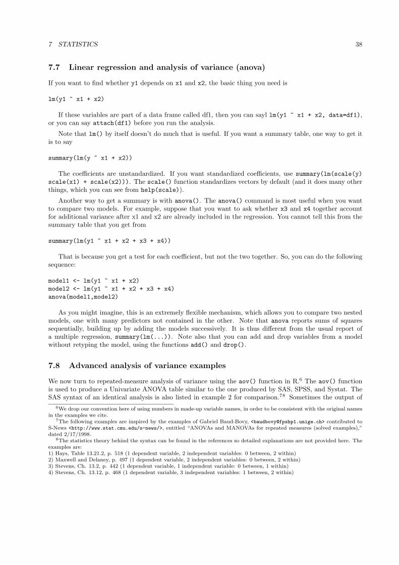
7 STATISTICS 38

7.7 Linear regression and analysis of variance (anova)

If you want to find whether y1 depends on x1 and x2, the basic thing you need is

lm(y1 ~ x1 + x2)

If these variables are part of a data frame called df1, then you can sayl lm(y1 ~ x1 + x2, data=df1),or you can say attach(df1) before you run the analysis.

Note that lm() by itself doesn’t do much that is useful. If you want a summary table, one way to get itis to say

summary(lm(y ~ x1 + x2))

The coefficients are unstandardized. If you want standardized coefficients, use summary(lm(scale(y)scale(x1) + scale(x2))). The scale() function standardizes vectors by default (and it does many otherthings, which you can see from help(scale)).

Another way to get a summary is with anova(). The anova() command is most useful when you wantto compare two models. For example, suppose that you want to ask whether x3 and x4 together accountfor additional variance after x1 and x2 are already included in the regression. You cannot tell this from thesummary table that you get from

summary(lm(y1 ~ x1 + x2 + x3 + x4))

That is because you get a test for each coefficient, but not the two together. So, you can do the followingsequence:

model1 <- lm(y1 ~ x1 + x2)model2 <- lm(y1 ~ x1 + x2 + x3 + x4)anova(model1,model2)

As you might imagine, this is an extremely flexible mechanism, which allows you to compare two nestedmodels, one with many predictors not contained in the other. Note that anova reports sums of squaressequentially, building up by adding the models successively. It is thus different from the usual report ofa multiple regression, summary(lm(...)). Note also that you can add and drop variables from a modelwithout retyping the model, using the functions add() and drop().

7.8 Advanced analysis of variance examples

We now turn to repeated-measure analysis of variance using the aov() function in R.6 The aov() functionis used to produce a Univariate ANOVA table similar to the one produced by SAS, SPSS, and Systat. TheSAS syntax of an identical analysis is also listed in example 2 for comparison.78 Sometimes the output of

6We drop our convention here of using numbers in made-up variable names, in order to be consistent with the original namesin the examples we cite.

7The following examples are inspired by the examples of Gabriel Baud-Bovy, <[email protected]> contributed toS-News <http://www.stat.cmu.edu/s-news/>, entitled “ANOVAs and MANOVAs for repeated measures (solved examples),”dated 2/17/1998.

8The statistics theory behind the syntax can be found in the references so detailed explanations are not provided here. Theexamples are:1) Hays, Table 13.21.2, p. 518 (1 dependent variable, 2 independent variables: 0 between, 2 within)2) Maxwell and Delaney, p. 497 (1 dependent variable, 2 independent variables: 0 between, 2 within)3) Stevens, Ch. 13.2, p. 442 (1 dependent variable, 1 independent variable: 0 between, 1 within)4) Stevens, Ch. 13.12, p. 468 (1 dependent variable, 3 independent variables: 1 between, 2 within)

7 STATISTICS 39

aov() is different from the output of a GLM procedure in SAS and SPSS. This may seem confusing forsomeone who is more familiar with SAS and SPSS than with R. We will use example 1 below to show howthis can happen and what we can do to find a suitable alternative solution. We may need to use a linearmixed-effects models approach using lme() instead of repeated-measures ANOVA using aov().

7.8.1 Example 1: Mixed Models Approach to Within-Subject Factors (Hays, 1988, Table13.21.2, p. 518)

We use the data in Hays (1988) to describe how to carry out repeated-measures ANOVA with R. The exampleis simplified as follows. Suppose a psychologist is asked to conduct a study to help design the control panelof a machine that delivers medicine by intravenous infusion. The main purpose of the study is to find thebest shape and color of the buttons on the control panel to improve efficiency and prevent potential errors.The psychologist wants to know how quickly users (physicians) respond to buttons of different colors andshapes. Suppose that the psychologist hypothesizes that bright colors are easier to see than dark colors sothe users respond to them faster. In addition, she thinks that users can spot circles faster than squares.These hypotheses may seem trivial, but they involve the same statistical techniques that can be extendedto more complicated experiments.

The psychologists knows that she will not be able to recruit many physicians to run the test apparatus.Thus she wants to collect as many test results as possible from each participating physician. Each participantworks with the test apparatus four times, one with round red buttons, one with square red buttons, onewith round gray buttons, and one with square gray buttons. Here the users only try each arrangement once,but the psychologist could ask them to repeat the tests several times in random order to get a more stableresponse time. In that case she would have another effect she may choose to test (repetition, or the effect oflearning).

In psychology, an experimental design like this is often called a “repeated measures” design because eachrespondent gives several responses. It is also referred to as a within-subject design because the measurementsare made repeatedly within individual subjects. The variables shape and color are therefore called within-subject variables. It is possible to do the experiment between subjects. Each data point comes from adifferent physician. A completely between-subject experiment is also called a randomized design. However,the experimenter would need to recruit four times as many physicians, which is not efficient.

This example has 2 within-subject variables and no between subject variables:

• one dependent variable: time required to solve the puzzles

• one random effect: subject (see Hays for reasons why)

• 2 within-subject fixed effects: shape (2 levels), color (2 levels)

We first enter the reaction time data into a vector data1. Then we transform data1 into appropriateformat for the repeated analysis of variance using aov().

data1<-c(49,47,46,47,48,47,41,46,43,47,46,45,48,46,47,45,49,44,44,45,42,45,45,40,49,46,47,45,49,45,41,43,44,46,45,40,45,43,44,45,48,46,40,45,40,45,47,40) # across subjects then conditions

We can take a look at the data in a layout that is easier to read. Each subject takes up a row in the datamatrix.

7 STATISTICS 40

> matrix(data1, ncol= 4, dimnames =+ list(paste("subj", 1:12), c("Shape1.Color1", "Shape2.Color1",+ "Shape1.Color2", "Shape2.Color2")))

Shape1.Color1 Shape2.Color1 Shape1.Color2 Shape2.Color2subj 1 49 48 49 45subj 2 47 46 46 43subj 3 46 47 47 44subj 4 47 45 45 45subj 5 48 49 49 48subj 6 47 44 45 46subj 7 41 44 41 40subj 8 46 45 43 45subj 9 43 42 44 40subj 10 47 45 46 45subj 11 46 45 45 47subj 12 45 40 40 40

Next we use the data.frame() function to create a data frame Hays.df that is appropriate for the aov()function.

Hays.df <- data.frame(rt = data1,subj = factor(rep(paste("subj", 1:12, sep=""), 4)),shape = factor(rep(rep(c("shape1", "shape2"), c(12, 12)), 2)),color = factor(rep(c("color1", "color2"), c(24, 24))))

The experimenter is interested in knowing if the shape (shape) and the color (color) of the buttonsaffect the reaction time (rt). The syntax is:

aov(rt ~ shape * color + Error(subj/(shape * color)), data=Hays.df)

The model formula, rt ~ shape * color + Error(subj/(shape * color)), can be divided into twoparts. The first part, rt ~ shape * color, states that reaction time is affected by the shapes and colorsof the buttons. The asterisk is a shorthand for shape + color + shape:color, representing the shape andcolor main effects and the shape by color interaction. The second part, Error(subj/(shape * color)), isvery important for getting the appropriate statistical tests. We will first explain what the syntax means,then we will explain why we do it this way.

The Error(subj/(shape * color)) statement is used to separate the residual sums of squares intoseveral components (called error strata). The statement is equivalent to Error(subj + subj:shape +subj:color + subj:shape:color), meaning that we want to separate the following error terms: one forsubject, one for subject by shape interaction, one for subject by color interaction, and one for subject byshape by color interaction.

This syntax generates the appropriate tests for the within-subject variables shape and color. You get

> summary(aov(rt ~ shape * color + Error(subj/(shape*color)), data=Hays.df))

Error: subjDf Sum Sq Mean Sq F value Pr(>F)

Residuals 11 226.500 20.591

7 STATISTICS 41

Error: subj:shapeDf Sum Sq Mean Sq F value Pr(>F)

shape 1 12.0000 12.0000 7.5429 0.01901 *Residuals 11 17.5000 1.5909---Signif. codes: 0 ‘***’ 0.001 ‘**’ 0.01 ‘*’ 0.05 ‘.’ 0.1 ‘ ’ 1

Error: subj:colorDf Sum Sq Mean Sq F value Pr(>F)

color 1 12.0000 12.0000 13.895 0.003338 **Residuals 11 9.5000 0.8636---Signif. codes: 0 ‘***’ 0.001 ‘**’ 0.01 ‘*’ 0.05 ‘.’ 0.1 ‘ ’ 1

Error: subj:shape:colorDf Sum Sq Mean Sq F value Pr(>F)

shape:color 1 1.200e-27 1.200e-27 4.327e-28 1Residuals 11 30.5000 2.7727

Note that the shape effect is tested against the residuals of the subject by shape interaction, shown inthe subj:shape error stratum. Similarly, the color effect is tested against subject by color stratum. Thelast error stratum with Error: subj:shape:color offers a test of the shape:color interaction.

Random vs. Fixed Effects In this simplified example we have one “random” subject effect (subj)and two “fixed” experimental manipulations (color and shape). In a repeated-measures design where thewithin-subject factors are considered fixed effects and the only random effect comes from subjects, thewithin-subject factors are tested against their interaction with the random subject effect. According to Hays(1988), the appropriate F tests are the following:

F(shape in subj) = MS(shape) / MS(shape : subj) = 7.543

F(color in subj) = MS(color) / MS(color : subj) = 13.895

Without going into the details, we can still understand the distinction between a random and a fixedeffect. Take the fixed shape effect as an example, the psychologist only wants to compare the reactiontime differences between round and square buttons. She is not concerned about generalizing the effect tobuttons of other shapes. In this case the number of possible shapes is fixed to two—round and square. Thereaction time differences between the two conditions do not generalize beyond these two shapes. Similarly,the variable color is also considered fixed (again the effect not generalizable to colors other than red andgray).

When color and shape are both considered fixed, they are tested against the subj:color and subj:shapemean squares, respectively. The Error() function allows you to do these comparisons. In this example theonly random effect is the subj effect. The 12 subjects reported here belong to a random sample of numerousother potential users of the device. The study would not be very useful without this generalizability becausethe results of the experiments would only apply to these particular 12 test subjects.

Without the Error(subj/(shape * color)) formula, you get the wrong statistical tests. Note thatboth color and shape are tested against a common entry called “Residuals”, which is the sum of all thepieces of residuals in the previous output of Error(subj/(shape * color)), with 11 degrees of freedom ineach of the four error strata.

> summary(aov(rt ~ shape*color, data=hays.df))Df Sum Sq Mean Sq F value Pr(>F)

7 STATISTICS 42

shape 1 12.000 12.000 1.8592 0.1797color 1 12.000 12.000 1.8592 0.1797shape:color 1 4.399e-29 4.399e-29 6.816e-30 1.0000Residuals 44 284.000 6.455

Note about Error() What goes inside the Error() statement, and the order in which they arearranged, are important in ensuring correct statistical tests. Suppose you replaced the asterisk insideError(subj/(shape * color)) with a plus sign, you got Error(subj/(shape + color)) instead:

> summary(aov(rt ~ shape * color + Error(subj/(shape + color)),data=Hays.df))

[identical output as before ... snipped ]


shape:color 1 1.185e-27 1.185e-27 4.272e-28 1Residuals 11 30.5000 2.7727

Note that Error() lumps the shape:color and subj:shape:color sums of squares into a “Within”error stratum. The “Residuals” in the Within stratum is actually the last piece of sum of square in theprevious output (subj:shape:color). This Error(subj/(shape + color)) syntax gives you the wrongstatistics when you have more than two within-subject variables. We will return to this point later.

There is a subtle detail in the Error(subj/(shape * color)) syntax that is worth noticing. For reasonsthat will become clearer in the next section, the forward slash (the / in subj/(shape * color)) tells aov()that the shape and color of the buttons are actually nested within individual subjects. That is, the changesin response time due to shape and color should be considered within the subjects.

Unbalanced (Nonorthogonal) Designs We will conclude the first example by introducing a com-mon complication in repeated-measures ANOVA that involves uneven cell size. In the example above, thereare four possible combinations of shape and color, each containing exactly 12 observations. We call thisdesign “balanced” because an equal number of observations is found in every combination (or a “cell”) ofthe design. A balanced design is also called an “orthogonal” design. In a balanced design, the aov() syntaxabove produces exactly the same univariate test statistics as SPSS and SAS. However, often the cell size isnot even, making the design “unbalanced” or “nonorthogonal”. This complication may be due to participantattrition or a post-hoc grouping factor that was not originally allotted the same number of participants. Forexample, the experimenter may stratify the design by gender, that is, by recruiting an equal number offemale and male physicians in the study. But later on the experimental may decide to try analyzing thereaction time by years of professional experience as the between-subject factor.

When a design is “unbalanced”, its aov() test statistics may look very different from those obtainedin SPSS and SAS. The reason is because statistical packages like the GLM procedure in SPSS adjusts thedefault Type III Sums of Squares by the harmonic mean of the unbalanced cell sizes. The adjustment isdiscussed in Maxwell and Delaney (1990, pp. 271-297).

SPSS produces the same output as R if the user tells SPSS to calculate the Type I SS (SSTYPE(1)) orType II SS (SSTYPE(2)) instead of the default SSTYPE(3). As shown in Maxwell and Delaney (1990), thecalculations of SS1 and SS2 do not involve the harmonic mean. Maxwell and Delaney discuss the pros andcons of each type of Sums of Squares. Apparently SPSS and SAS think that the harmonic mean SS3 is theright analysis. Afterall, the SS3 is in general what a behaivoral scientist seeks. Readers who are interestedin the distinctions between the different types of SS can find a discussion in Maxwell and Delaney (1990).The example aov() analysis below can be compared with the results of SPSS using SSTYPE(2).

# add one unbalanced between-subject variable

7 STATISTICS 43

# n=8 in grp 1; 4 in grp 2Hays.df$grp <- factor(rep(c(1,1,1,1,1,1,1,1,2,2,2,2), 4))summary(aov(rt ~ grp*color*shape + Error(subj/shape+color), data=Hays.df))

GLMSh1Col1 Sh2Col1 Sh1Col2 Sh2Col2 BY grp/WSFACTOR = color 2 Polynomial shape 2 Polynomial/METHOD = SSTYPE(2)/CRITERIA = ALPHA(.05)/WSDESIGN = color shape color*shape/DESIGN = grp .

7.8.2 Example 2: Maxwell and Delaney, p. 497

It is the same design as in the previous example, with two within and a subject effect. We repeat the sameR syntax, then we include the SAS GLM syntax for the same analysis. Here we have:

one dependent variable: reaction time

two independent variables: visual stimuli are tilted at 0, 4, and 8 degrees; with noise absent or present.Each subject responded to 3 tilt x 2 noise = 6 trials.

The data are entered slightly differently; their format is like what you would usually do with SAS, SPSS,and Systat.

MD497.dat <- matrix(c(420, 420, 480, 480, 600, 780,420, 480, 480, 360, 480, 600,480, 480, 540, 660, 780, 780,420, 540, 540, 480, 780, 900,540, 660, 540, 480, 660, 720,360, 420, 360, 360, 480, 540,480, 480, 600, 540, 720, 840,480, 600, 660, 540, 720, 900,540, 600, 540, 480, 720, 780,480, 420, 540, 540, 660, 780),ncol = 6, byrow = T) # byrow=T so the matrix’s layout is exactly like this

Next we transform the data matrix into a data frame.

MD497.df <- data.frame(rt = as.vector(MD497.dat),subj = factor(rep(paste("s", 1:10, sep=""), 6)),deg = factor(rep(rep(c(0,4,8), c(10, 10, 10)), 2)),noise = factor(rep(c("no.noise", "noise"), c(30, 30))))

Then we test the main effects and the interaction in one aov() model. The syntax is the same as in theHays example:

taov <- aov(rt ~ deg * noise + Error(subj / (deg * noise)), data=MD497.df)summary(taov)

7 STATISTICS 44

The results obtained with R can be compared with those obtained using SAS or SPSS. The following SASGLM syntax carries out the same univariate analysis, plus some multivariate tests. Maxwell and Delaneysummarized the conditions under which one wants to trust the multivariate results more than the univariateresults. In SAS, each row contains the data from one subject, across 3 degrees of tilt and two levels of noise.The GLM syntax has a class option where the between-subject factors are listed (if any).

data rt1;input deg0NA deg4NA deg8NA deg0NP deg4NP deg8NP;cards;420 420 480 480 600 780420 480 480 360 480 600480 480 540 660 780 780420 540 540 480 780 900540 660 540 480 660 720360 420 360 360 480 540480 480 600 540 720 840480 600 660 540 720 900540 600 540 480 720 780480 420 540 540 660 780;

proc glm data=rt1;model deg0NA deg4NA deg8NA deg0NP deg4NP deg8NP = ;repeated noise 2 (0 1), degree 3 (0 4 8) / summary ;run;

7.8.3 Example 3: More Than Two Within-Subject Variables

Earlier we noted that Error(subj/(shape * color)), which uses an asterisk to connect shape and color,produces detailed breakdown of the variance components. The Error(subj/(shape + color)) statementprints out what you specifically ask for and lumps the remainder into a “Within” stratum. If you have morethan two within-subject fixed effects, the latter will produce some undesirable side effects.

The next hypothetical example 9 shows that aov(a * b * c + Error(subj/(a+b+c))) does not giveyou the appropriate statistical tests for the two-way interactions among factors a, b, and c. The problem isbecause Error() lumps everything other than Error: subj:a, Error: subj:b, and Error: subj:c into acommon entry of residuals. The S Model book by Chambers and Hastie contains some technical details thatexplains this behavior.

subj <- gl(10, 32, 320) # 10 subjects, each tested 32 times, total length 320a <- gl(2, 16, 320) # first 16 trials with a1 then next 16 with a2b <- gl(2, 8, 320) # first 8 triasl with b1, then next 8 with b2, etc.c <- gl(2, 4, 320)x <- rnorm(320)d1 <- data.frame(subj, a, b, c, x)d2 <- aggregate(x, list(a = a, b = b, c = c, subj = subj), mean)summary(a1 <- aov(x ~ a * b * c + Error(subj/(a*b*c)), d2))summary(a2 <- aov(x ~ a * b * c + Error(subj/(a+b+c)), d2))summary(a3 <- aov(x ~ a * b * c + Error(subj/(a*b*c)), d1))

9contributed by Christophe Pallier

7 STATISTICS 45

7.8.4 Example 4: Stevens, 13.2, p.442; a simpler design with only one within variable

data <- c(30,14,24,38,26,28,18,20,34,28,16,10,18,20,14,34,22,30,44,30)Stv.df <- data.frame(rt=data,subj = factor(rep(paste("subj", 1:5, sep=""), 4)),drug = factor(rep(paste("drug", 1:4, sep=""), c(5,5,5,5))))

We only have one within-subject variable (drug) so that the syntax is simply drug nested within subject.

summary(aov(rt ~ drug + Error(subj/drug), data = Stv.df))

7.8.5 Example 5: Stevens pp. 468 – 474 (one between, two within)

The original data came from Elashoff (1981).10 It is a test of drug treatment effect by one between-subjectfactor: group (two groups of 8 subjects each) and two within-subject factors: drug (2 drugs) and dose (3doses).

Ela.mat <-matrix(c(19,22,28,16,26,22,11,19,30,12,18,28,20,24,24,24,22,29,21,25,25,15,10,26,18,24,29,19,26,28,17,23,28,15,23,22,20,23,23,26,21,28,14,20,29,25,29,29,16,20,24,30,34,36,26,26,26,24,30,32,22,27,23,33,36,45,16,18,29,27,26,34,19,21,20,22,22,21,20,25,25,29,29,33,21,22,23,27,26,35,17,20,22,23,26,28), nrow = 16, byrow = T)

We first put them in a multivariate format, using the cbind.data.frame() function.

Ela.mul <- cbind.data.frame(subj=1:16, gp=factor(rep(1:2,rep(8,2))), Ela.mat)dimnames(Ela.mul)[[2]] <-c("subj","gp","d11","d12","d13","d21","d22","d23") # d12 = drug 1, dose 2

Here is the command for transferring it to the univariate format.10“Data for the panel session in software for repeated measures analysis of variance.” Proceedings of the Statistical Computing

Section of the American Statistical Association.

7 STATISTICS 46

Ela.uni <- data.frame(effect = as.vector(Ela.mat),subj = factor(paste("s", rep(1:16, 6), sep="")),gp = factor(paste("gp", rep(rep(c(1, 2), c(8,8)), 6), sep="")),drug = factor(paste("dr", rep(c(1, 2), c(48, 48)), sep="")),dose=factor(paste("do", rep(rep(c(1,2,3), rep(16, 3)), 2), sep="")),row.names = NULL)

The next command performs the correct tests of all effects. We use Error(subj/(dose*drug)) to testgp, drug, dose and their interactions. Worth noting is that R knows that the gp effect goes with the subjecterror stratum, although we did not mention gp in the Error() statement.

summary(aov(effect ~ gp * drug * dose + Error(subj/(dose*drug)), data=Ela.uni))

7.8.6 Other Useful Functions for ANOVA

As we discussed earlier, we can use the tapply() function to calculate the means across various conditions.We can think of it as using one statement to run the mean() function 12 times! The output matrix is veryuseful for plotting.

tapply(Ela.uni$effect, IND = list(Ela.uni$gp, Ela.uni$drug, Ela.uni$dose),FUN = mean)

We can also easily custom design a function se() to calculate the standard error for the means. R doesnot have a built-in function for that purpose, but there is really no need because the standard error is justthe square root (R has the sqrt() function) of the variance (var()), divided by the number of observations(length()). We can use one line of tapply() to get all standard errors. The se() makes it easy to find theconfidence intervals for those means. Later we will demonstrate how to use the means and standard errorswe got from tapply() to plot the data.

se <- function(x){

y <- x[!is.na(x)] # remove the missing valuessqrt(var(as.vector(y))/length(y))

}

In R, we not only can use the built-in functions such as aov() to do the analyses, we can also takeadvantage of R’s flexibility and do many analyses by hand. The following examples demonstrate that someof the ANOVA tests we did earlier with the aov() function can also be done manually with contrasts.

1. We can use the following contrast to test the group effect. On the left hand side of the aov() model,we use matrix multiplication (%*%) to apply the contrast (contr) to each person’s 6 data points. As aresult, each person’s 6 data points become one number that is actually the person’s total score summedacross all conditions. The matrix multiplication is the same as doing 1 * d11 + 1 * d12 + 1 * d13+ 1 * d21 + 1 * d22 + 1 * d23 for each person.

Then we use the aov() function to compare the total scores across the two groups. We can verifythat in this output the F statistic for the gp marginal effect is exactly the same as the one in the theprevious aov(... Error()) output, although the sums of squares are different because the contrastis not scaled to length 1.

7 STATISTICS 47

contr <- matrix(c(1,1,1,1,1,1), ncol = 1)

taov <- aov(cbind(d11,d12,d13,d21,d22,d23) %*% contr ~ gp, data = Ela.mul)summary(taov, intercept = T)

2. The following contrast, when combined with the aov() function, will test the drug main effect anddrug:group interaction. The contrast c(1, 1, 1, -1, -1, -1) applies positive 1’s to columns 1:3 andnegative 1’s to columns 4:6. Columns 1:3 contain the data for drug 1 and 4:6 for drug 2, respectively.So the contrast and the matrix multiplication generates a difference score between drugs 1 and 2. Whenwe use aov() to compare this difference among two groups, we actually test the drug:gp interaction.

contr <- matrix(c(1,1,1,

-1,-1,-1), ncol = 1)

tmp<-aov(cbind(d11,d12,d13,d21,d22,d23) %*% contr ~ gp, Ela.mul)summary(tmp,intercept= T)

3. The next contrast, when combined with the manova() function in R-1.2.0 or later, tests the dosemain effect and the dose:group interaction. The first contrast c(1, 0, -1, 1, 0, -1) tests if thedifference between dose 1 and dose 3 are statistically significant across groups; and the second contrastc(0, 1, -1, 0, 1, -1) tests the difference between dose 2 and dose 3 across two groups. Whentested simultaneously with manova(), we get

contr <- matrix(c(1, 0,0, 1,

-1,-1,1, 0,0, 1,

-1,-1), nrow = 6, byrow = T)

tmp <- manova(cbind(d11,d12,d13,d21,d22,d23) %*% contr ~ gp, Ela.mul)summary(tmp, test="Wilks", intercept = T)

4. Another manova() contrast, which tests drug:dose interaction and drug:dose:group interaction.

contr <- matrix(c(1,-1,0, 2,

7 STATISTICS 48

-1,-1,-1, 1,0,-2,1, 1), nrow = 6, byrow = T)

tmp<-manova(cbind(d11,d12,d13,d21,d22,d23) %*% contr ~ gp, Ela.mul)summary(tmp, test="Wilks", intercept = T)

7.8.7 Graphics with error bars

Next we will demonstrate how to use R’s powerful graphics functions to add error bars to a plot. The exampleuses the Elashoff example discussed earlier. In this example we will briefly show how visual representationscompliment the statistical tests. We use R’s jpg() graphics driver to generate a graph that can be viewed bya web browser. The command syntax may appear intimidating for beginners, but it is worth the increasedefficiency in the long run.

You can also use the postscript() graphics driver to generate presentation-quality plots. PostScriptfiles can be transformed into PDF format so that nowadays the graphs generated by R can be viewed andprinted by virtually anyone.11

Typically the graphs are first generated interactively with drivers like X11(), then the commands aresaved and edited into a script file. A command syntax script eliminates the need to save bulky graphic files.

First we start the graphics driver jpg() and name the file where the graph(s) will be saved.

attach(Ela.uni)jpeg(file = "ElasBar.jpg")

Then we find the means, the standard errors, and the 95% confidence bounds of the means.

tmean <- tapply(effect, IND = list(gp, drug, dose), mean)tse <- tapply(effect, IND = list(gp, drug, dose), se)tbarHeight <- matrix(tmean, ncol=3)dimnames(tbarHeight) <- list(c("gp1dr1","gp2dr1","gp1dr2","gp2dr2"),

c("dose1","dose2" ,"dose3"))tn <- tapply(effect, IND = list(gp, drug, dose), length)tu <- tmean + qt(.975, df=tn-1) * tse # upper bound of 95% confidence int.tl <- tmean + qt(.025, df=tn-1) * tse # lower boundtcol <- c("blue", "darkblue", "yellow", "orange") # color of the bars

After all the numbers are computed, we start building the barplot. First we plot the bars without theconfidence intervals, axes, labels, and tick marks. Note that the barplot() function returns the x-axis valuesat where the center of the bars are plotted. Later we will use the values in tbars to add additional pieces.

tbars <- barplot(height=tbarHeight, beside=T, space=c(0, 0.5),ylab="", xlab="", axes=F, names.arg=NULL, ylim=c(-15, 40),col=tcol)

Then we add the 95% confidence intervals of the means to the bars.11One converter is ps2pdf, or try GhostScript.

7 STATISTICS 49

segments(x0=tbars, x1=tbars, y0=tl, y1=tu)segments(x0=tbars-.1, x1=tbars+0.1, y0=tl, y1=tl) # lower whiskerssegments(x0=tbars-.1, x1=tbars+0.1, y0=tu, y1=tu) # upper whiskers

The axes labels are added.

axis(2, at = seq(0, 40, by=10), labels = rep("", 5), las=1)tx <- apply(tbars, 2, mean) # center positions for 3 clusters of bars

We plot the horizontal axis manually so that we can ask R to put things at exactly where we want them.

segments(x0=0, x1=max(tbars)+1.0, y0=0, y1=0, lty=1, lwd = 2)text(c("Dose 1", "Dose 2", "Dose 3"), x = tx, y = -1.5, cex =1.5)mtext(text=seq(0,40,by=10), side = 2, at = seq(0,40,by=10),

line = 1.5, cex =1.5, las=1)mtext(text="Drug Effectiveness", side = 2, line = 2.5, at = 20, cex =1.8)

Finally we want to plot the legend of the graph manually. R also has a legend() function, although lessflexible.

tx1 <- c(0, 1, 1, 0)ty1 <- c(-15, -15, -13, -13)polygon(x=tx1, y=ty1, col=tcol[1])polygon(x=tx1, y=ty1 + 2.5, col=tcol[2]) # 2nd, moved 2.5 points uppolygon(x=tx1, y=ty1 + 5, col=tcol[3]) # 3rdpolygon(x=tx1, y=ty1 + 7.5, col=tcol[4]) # last

Finally, we add the legend labels for the filled rectangles.

text(x = 2.0, y = -14, labels="group 1, drug 1", cex = 1.5, adj = 0)text(x = 2.0, y = -11.5, labels="group 2, drug 1", cex = 1.5, adj = 0)text(x = 2.0, y = -9, labels="group 1, drug 2", cex = 1.5, adj = 0)text(x = 2.0, y = -6.5, labels="group 2, drug 2", cex = 1.5, adj = 0)

The greatest effectiveness is attained by subjects in group 2 when drug 2 is given. This suggests a groupby drug interaction, which is confirmed by the aov() results outlined earlier. It also indicates an increasingeffectiveness from dose 1 to 3, which is also confirmed by the statistics.

7.8.8 Another way to do error bars using plotCI()

The gplots library has a function plotCI(), which does confidence intervals for plots. Here is an example,which is Figure 1 in http://journal.sjdm.org/06137/jdm06137.htm. Note the use of a small horizontaloffset (−.01) so that the error bars do not overlap. The font “NimbusSan” is supposed to fit well with TimesRoman.

library("gplots")m.pg <- c(-2.6400, 3.6000, 6.0000, 3.6800, 5.4400)se.pg <- c(1.71938, 1.86548, 1.74738, 1.94484, 1.83492)m.pl <- c(-4.9600, -3.7600, -2.3200, -.1600, 6.5600)

7 STATISTICS 50

se.pl <- c(1.47024, 1.72170, 1.79139, 1.36587, 1.56852)

postscript(file="fig1.eps",family="NimbusSan",width=8,height=8,horiz=F,pointsize=18,paper="special")

plotCI(y=c(m.pg,m.pl),x=c(c(1:5)-.01,c(1:5)+.01),uiw=c(se.pg,se.pl),ylim=c(-6,8),ylab="Net IGT score",xlab="Block",lty=rep(c(1,2),c(5,5)))

lines(y=m.pg,x=c(1:5)-.01,lty=1)lines(y=m.pl,x=c(1:5)+.01,lty=2)legend(3.6,-3.7,legend=c("Prior gain","Prior loss"),lty=c(1,2))dev.off()

7.9 Use Error() for repeated-measure ANOVA

In this section we give an intuitive explanation to the use of the Error() statement for repeated-measureanalysis of variance. These explanations are different than what are typically covered in advanced textbooks.The conventional method focuses on deriving the appropriate error terms for specific statistical tests. Weuse an intuitive method, which will show that using Error() inside an aov() function is actually the sameas performing t-tests using contrasts.

The conventional explanation is computationally and theoretically equivalent to what we are about tosummarize. Detailed theoretical explanations can be found in most advanced textbooks, including the bookby Hoaglin, Mosteller, and Tukey (1991). Explanations of the technical details can be found in the book byChambers and Hastie (1992).

We first review Analysis of Variance using a method commonly seen in most introductory textbooks.This method uses an ANOVA table to describes how much of the total variability is accounted for by all therelated variables. An ANOVA table is exactly what aov() does for you. We first apply this method to theHays.df data described earlier (but repeated here), then we use the ANOVA table to explain why we mustadd the Error() statement in an aov() command in order to get the appropriate significance tests. Finallywe draw a connection between Error() and specific t-tests tailored for repeated-measure data.

7.9.1 Basic ANOVA table with aov()

The aov() function generates a basic ANOVA table if Error() is not inserted. Applying a simple aov() tothe Hays.df data, you get an ANOVA table like the following:

summary(aov(rt ~ subj * color * shape, data = Hays.df))Df Sum Sq Mean Sq

subj 11 226.500 20.591color 1 12.000 12.000shape 1 12.000 12.000subj:color 11 9.500 0.864subj:shape 11 17.500 1.591color:shape 1 1.493e-27 1.493e-27subj:color:shape 11 30.500 2.773

R analyzes how reaction time differs depending on the subjects, color and the shape of the stimuli. Also,you can have R tell you how they interact with one another. A simple plot of the data may suggest aninteraction between color and shape. A color:shape interaction occurs if, for example, the color yellow iseasier to recognize than red when it comes in a particular shape. The subjects may recognize yellow squaresmuch faster than any other color and shape combinations. Therefore the effect of color on reaction time isnot the same for all shapes. We call this an interaction.

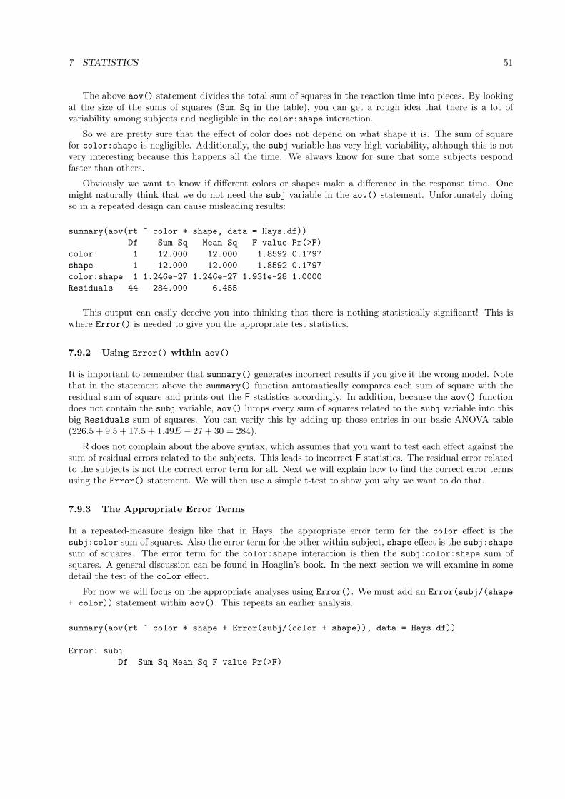
7 STATISTICS 51

The above aov() statement divides the total sum of squares in the reaction time into pieces. By lookingat the size of the sums of squares (Sum Sq in the table), you can get a rough idea that there is a lot ofvariability among subjects and negligible in the color:shape interaction.

So we are pretty sure that the effect of color does not depend on what shape it is. The sum of squarefor color:shape is negligible. Additionally, the subj variable has very high variability, although this is notvery interesting because this happens all the time. We always know for sure that some subjects respondfaster than others.

Obviously we want to know if different colors or shapes make a difference in the response time. Onemight naturally think that we do not need the subj variable in the aov() statement. Unfortunately doingso in a repeated design can cause misleading results:

summary(aov(rt ~ color * shape, data = Hays.df))Df Sum Sq Mean Sq F value Pr(>F)

color 1 12.000 12.000 1.8592 0.1797shape 1 12.000 12.000 1.8592 0.1797color:shape 1 1.246e-27 1.246e-27 1.931e-28 1.0000Residuals 44 284.000 6.455

This output can easily deceive you into thinking that there is nothing statistically significant! This iswhere Error() is needed to give you the appropriate test statistics.

7.9.2 Using Error() within aov()

It is important to remember that summary() generates incorrect results if you give it the wrong model. Notethat in the statement above the summary() function automatically compares each sum of square with theresidual sum of square and prints out the F statistics accordingly. In addition, because the aov() functiondoes not contain the subj variable, aov() lumps every sum of squares related to the subj variable into thisbig Residuals sum of squares. You can verify this by adding up those entries in our basic ANOVA table(226.5 + 9.5 + 17.5 + 1.49E − 27 + 30 = 284).

R does not complain about the above syntax, which assumes that you want to test each effect against thesum of residual errors related to the subjects. This leads to incorrect F statistics. The residual error relatedto the subjects is not the correct error term for all. Next we will explain how to find the correct error termsusing the Error() statement. We will then use a simple t-test to show you why we want to do that.

7.9.3 The Appropriate Error Terms

In a repeated-measure design like that in Hays, the appropriate error term for the color effect is thesubj:color sum of squares. Also the error term for the other within-subject, shape effect is the subj:shapesum of squares. The error term for the color:shape interaction is then the subj:color:shape sum ofsquares. A general discussion can be found in Hoaglin’s book. In the next section we will examine in somedetail the test of the color effect.

For now we will focus on the appropriate analyses using Error(). We must add an Error(subj/(shape+ color)) statement within aov(). This repeats an earlier analysis.

summary(aov(rt ~ color * shape + Error(subj/(color + shape)), data = Hays.df))

Error: subjDf Sum Sq Mean Sq F value Pr(>F)

7 STATISTICS 52

Residuals 11 226.500 20.591

Error: subj:colorDf Sum Sq Mean Sq F value Pr(>F)

color 1 12.0000 12.0000 13.895 0.003338 **Residuals 11 9.5000 0.8636---Signif. codes: 0 ‘***’ 0.001 ‘**’ 0.01 ‘*’ 0.05 ‘.’ 0.1 ‘ ’ 1

Error: subj:shapeDf Sum Sq Mean Sq F value Pr(>F)

shape 1 12.0000 12.0000 7.5429 0.01901 *Residuals 11 17.5000 1.5909---Signif. codes: 0 ‘***’ 0.001 ‘**’ 0.01 ‘*’ 0.05 ‘.’ 0.1 ‘ ’ 1


color:shape 1 1.139e-27 1.139e-27 4.108e-28 1Residuals 11 30.5000 2.7727

As we mentioned before, the Error(subj/(color * shape)) statement is the short hand for dividingall the residual sums of squares—in this case all subject-related sums of squares—into three error strata.

The Error() statement says that we want three error terms separated in the ANOVA table: one forsubj, subj:color, and subj:shape, respectively. The summary() and aov() functions are smart enoughto do the rest for you. The effects are arranged according to where they belong. In the output the coloreffect is tested against the correct error term subj:color, etc. If you add up all the Residuals entries inthe table, you will find that it is exactly 284, the sum of all subject-related sums of squares.

7.9.4 Sources of the Appropriate Error Terms

In this section we use simple examples of t-tests to demonstrate the need of the appropriate error terms.Rigorous explanations can be found in Edwards (1985) and Hoaglin, Mosteller, and Tukey (1991). We willdemonstrate that the appropriate error term for an effect in a repeated ANOVA is exactly identical to thestandard error in a t statistic for testing the same effect.

Let’s use the data in Hays (1988), which we show here again as hays.mat (See earlier example for howto read in the data).

hays.matShape1.Color1 Shape2.Color1 Shape1.Color2 Shape2.Color2

subj 1 49 48 49 45subj 2 47 46 46 43subj 3 46 47 47 44subj 4 47 45 45 45subj 5 48 49 49 48subj 6 47 44 45 46subj 7 41 44 41 40subj 8 46 45 43 45subj 9 43 42 44 40subj 10 47 45 46 45

7 STATISTICS 53

subj 11 46 45 45 47subj 12 45 40 40 40

In a repeated-measure experiment the four measurements of reaction time are correlated by design becausethey are from the same subject. A subject who responds quickly in one condition is likely to respond quicklyin other conditions as well.

To take into consideration these differences, the comparisons of reaction time should be tested withdifferences across conditions. When we take the differences, we use each subject as his/her own control. Sothe difference in reaction time has the subject’s baseline speed subtracted out. In the hays.mat data we testthe color effect by a simple t-test comparing the differences between the columns of “Color1” and “Color2.”

Using the t.test() function, this is done by

t.test(x = hays.mat[, 1] + hays.mat[, 2], y = hays.mat[, 3] + hays.mat[, 4],+ paired = T)

Paired t-test

data: hays.mat[, 1] + hays.mat[, 2] and hays.mat[, 3] + hays.mat[, 4]t = 3.7276, df = 11, p-value = 0.003338alternative hypothesis: true difference in means is not equal to 095 percent confidence interval:0.819076 3.180924

sample estimates:mean of the differences

2

An alternative is to test if a contrast is equal to zero, we talked about this in earlier sections:

t.test(hays.mat %*% c(1, 1, -1, -1))

One Sample t-test

data: hays.mat %*% c(1, 1, -1, -1)t = 3.7276, df = 11, p-value = 0.003338alternative hypothesis: true mean is not equal to 095 percent confidence interval:0.819076 3.180924

sample estimates:mean of x

2

This c(1, 1, -1, -1) contrast is identical to the first t-test. The matrix multiplication (the %*%operand) takes care of the arithmetic. It multiplies the first column by a constant 1, add column 2, thensubtract from that columns 3 and 4. This tests the color effect. Note that the p-value of this t test is thesame as the p-values for the first t test and the earlier F test.

It can be proven algebraically that the square of a t-statistic is identical to the F test for the sameeffect. So this fact can be used to double check the results. The square of our t-statistic for color is3.72762 = 13.895, which is identical to the F statistic for color.

Now we are ready to draw the connection between a t-statistic for the contrast and the F-statistic in anANOVA table for repeated-measure aov(). The t statistic is a ratio between the effect size to be tested

7 STATISTICS 54

and the standard error of that effect. The larger the ratio, the stronger the effect size. The formula can bedescribed as follows:

t =x̄1 − x̄2

s/√

n, (1)

where the numerator is the observed differences and the denominator can be interpreted as the expecteddifferences due to chance. If the actual difference is substantially larger than what you would expect, thenyou tend to think that the difference is not due to random chance.

Similarly, an F test contrasts the observed variability with the expected variability. In a repeated designwe must find an appropriate denominator by adding the the Error() statement inside an aov() function.

The next two commands show that the error sum of squares of the contrast is exactly identical to theResidual sum of squares for the subj:color error stratum.

tvec <- hays.mat %*% c(1, 1, -1, -1)/2sum((tvec - mean(tvec))^2)[1] 9.5

The sum of squares of the contrast is exactly 9.5, identical to the residual sum of squares for the correctF test. The scaling factor 1/2 is critical because it provides correct scaling for the numbers. By definition astatistical contrast should have a vector length of 1. This is done by dividing each element of the contrastvector by 2, turning it to c(1/2, 1/2, -1/2, -1/2). The scaling does not affect the t-statistics. But itbecomes important when we draw a connection between a t-test and an F test.

You get the standard error of the t-statistic if you do the following:

sqrt(sum((tvec - mean(tvec))^2 / 11) / 12)[1] 0.2682717

The first division of 11 is for calculating the variance; then you divide the variance by the sample size of12, take the square root, you have the standard error for the t-test. You can verify it by running se(hays.mat%*% c(1, 1, -1, -1)/2).

7.9.5 Verify the Calculations Manually

All the above calculations by aov() can be verified manually. This section summarizes some of the technicaldetails. This also gives you a flavor of how Analysis Of Variance can be done by matrix algebra. First were-arrange the raw data into a three-dimensional array. Each element of the array is one data point, and thethree dimensions are for the subject, the shape, and the color, respectively.

hays.A <- array(hays.dat, dim=c(12, 2, 2))dimnames(hays.A) <- list(paste("subj", 1:12, sep = ""),+ c("Shape1", "Shape2"), c("Color1", "Color2"))

Because at this point we want to solve for the effect of color, we use the apply() function to averagethe reaction time over the two shapes.

Ss.color <- apply(hays.A, c(1, 3), mean) # Ss x color: average across shape

Next we test a t-test contrast for the color effect, which is the same as t.test(Ss.color %*% c(1, -1)).Also note that the square of the t statistic is exactly the same as the F test.

7 STATISTICS 55

Contr <- c(1, -1)Ss.color.Contr <- Ss.color %*% Contrmean(Ss.color.Contr) / (sqrt(var(Ss.color.Contr) / length(Ss.color.Contr)))

[,1][1,] 3.727564

The above t-test compares the mean of the contrast against the standard error of the contrast, which issqrt(var(Ss.color.Contr) / length(Ss.color.Contr))

Now we can verify that the sum of square of the contrast is exactly the same as the error term when weuse aov() with the Error(subj:color) stratum.

sum((Ss.color.Contr - mean(Ss.color.Contr))^2)[1] 9.5

7.10 Sphericity

Sphericity is an assumption of repeated measure ANOVA. It means that the variance-covariance structure ofthe repeated measure ANOVA follows a certain pattern. In a repeated measure design, several measurementsare made to the same groups of subjects under different conditions (and/or at different time). Sphericity is,in a nutshell, that the variances of the differences between the repeated measurements should be about thesame. This is a complicated concept best explained with examples. Simple examples tend to oversimplifythings, because they often rely on idealized hypothetical data that rarely occur in real life. Although theirusefulness in relieving the burden of learning overcompensates for the over-simplification. In what followsthe example in section (cite the previous section???) is used again to explain what sphericity is, how tocalculate and test it, and what alternative statistics can be used if the sphericity assumption is not met.

7.10.1 Why is sphericity important?

Violations of the sphericity assumption lead to biased p-values. The alpha error of a test may be set at5%, but the test may be actually rejecting the null hypothesis 10% of the time. This raises doubts of theconclusions of the repeated measure ANOVA. Imagine a study about weight gains of new born babies atthe Intensive Care Unit. The weight of the babies is measured every day for a critical period of three days.On the average the babies gain 100 grams between days 1 and 2, and they gain 150 grams between days2 and 3. Sphericity says that the variance of the weight gain between days 1 and 2 should be about thesame as the variance of the weight gain between days 2 and 3 (and also between days 1 and 3). If not, thevariance observed between different time periods are confounded with the correlation of the measurementsmade at different time. Suppose the variance of the first weight gain is 20 and the variance of the secondweight gain is 100, then the measurements made at times 1 and 2 are likely to be correlated more closelythan measurements made at times 2 and 3. As a result the variance over the whole 3-day period (what isoften called the variance of the “time” effect in ANOVA jargon) fluctuates over time and is not reliable indescribing the overall growth pattern in critically ill babies.

In repeated measure experiments the same subjects are tested multiple times under different conditions.It is a good idea to check if the responses made under some conditions are correlated more closely thanresponses made under other conditions.

There is a statistic, The Greenhouse-Geisser epsilon ε, which measures by how much the sphericityassumption is violated. Epsilon is then used to adjust for the potential bias in the F statistic. Epsilon canbe 1, which means that the sphericity assumption is met perfectly. An epsilon smaller than 1 means that thesphericity assumption is violated. The further it deviates from 1, the worse the violation. In real life epsilonis rarely exactly 1. If it is not much smaller than 1, then we feel comfortable with the results of repeated

7 STATISTICS 56

measure ANOVA. Thus the question is how small is too small. We will get to that below. Additionally, wewill talk about two remedies when sphericity is violated: 1) correct for the p-value, and 2) use proceduresthat do not depend on sphericity, such as MANOVA.

7.10.2 How to estimate the Greenhouse-Geisser epsilon?

The Greenhouse-Geisser epsilon is derived from the variance-covariance matrix of the data. The MD497.datexample above involves a study where study subjects judged stimuli under 3 different angles of rotation, at0, 2, and 4 degrees angle from the horizontal. In this subsection we estimate the Greenhouse-Geisser epsilonassociated with the rotation of the stimuli. The 3 measurements of reaction time are stored in x0, x2, andx4, respectively.

x0 <- apply(MD497.dat[, c(1, 4)], 1, mean) # avg across noise present/absentx2 <- apply(MD497.dat[, c(2, 5)], 1, mean)x4 <- apply(MD497.dat[, c(3, 6)], 1, mean)

We need to first calculate the variance-covariance matrix of the 3 variables. The var() function calculatesthe variance-covariance matrix if the data are arranged in a matrix, like S <- var(cbind(x0, x2, x4)):

> var(cbind(x0, x2, x4))x0 x2 x4

x0 4090 3950 4350x2 3950 6850 6150x4 4350 6150 8850

The diagonal entries are the variances and the off diagonal entries are the covariances. From this variance-covariance matrix the ε statistic can be estimated:

ε̂ =k2(s̄ii − s̄)2

(k − 1)(∑∑

s2ij − 2k

∑s̄2

i. + k2s̄2),

where s̄ii is the mean of the entries on the main diagonal of S, which can be shown by mean(diag(S)) toequal 6596.667; s̄ is the mean of all entries, s̄i. is the mean of all entries in row i of S, and sij is the 9individual entries in the variance-covariance matrix.

S <- var(cbind(x0, x2, x4))k <- 3; D < - k^2 * ( mean ( diag ( S ) ) - mean ( S ) ) ^2N1 <- sum(S^2)N2 <- 2 * k * sum(apply(S, 1, mean)^2)N3 <- k^2 * mean(S)^2D / ((k - 1) * (N1 - N2 + N3))

Which returns [1] 0.9616365 for the value of ε̂. This value rounds to the 0.9616 value calculated by SAS(the SAS GLM syntax is provided above).

There are three important values of ε. It can be 1 when the sphericity is met perfectly. It can be aslow as ε = 1/(k − 1), which produces the lower bound of epsilon (the worst case scenario). The worst casescenario depends on k, the number of levels in the repeated measure factor. In this example k = 3. Eachsubject is tested under 3 different levels of stimuli rotation. Epsilon can be as low as 0.50 when k = 3. Notethat the sphericity assumption does not apply when k = 2. Another way to view it is that even the lowestepsilon is 1. Thus a repeated measure design with only 2 levels does not involve violations of the sphericityassumption.

7 STATISTICS 57

Adjustment of the F statistic can be made against either the estimated epsilon, in this case ε̂ = 0.962;or against the worst case epsilon of 0.50. It depends on how conservative one wants to be. If the cost offalsely rejecting the null hypothesis is high, then one may want to adjust against the worst possible (andvery conservative) epsilon. Both SPSS and SAS use the estimated value to make the Greenhouse-Geisseradjustment. The Greenhouse-Geisser adjustment made by SPSS and SAS is different from the adjustmentoriginally proposed by Greenhouse and Geisser (1959). Although the adjustment made by SPSS and SAS isconsidered more reasonable (Stevens, 1990).

The estimated epsilon is used to adjust the degrees of freedom associated with the F statistic from theunadjusted (k − 1) and (k − 1)(n − 1) to ε(k − 1) and ε(k − 1)(n − 1). Severe violations of the sphericityassumption (as ε̂ → 0) may decrease the degrees of freedom so much that the F statistic is no longerstatistically significant. The p-value associated with the adjusted F can be obtained from the pf() function.

¿From the previous aov() output we get an F statistic of 40.719 for the variable deg. The numeratordegree of freedom is (k−1) = 2 and the denominator degrees of freedom is (k−1)(n−1) = (3−1)(10−1) = 18.These can be verified with the output of the previous analysis. Suppose the value of epsilon is assigned toepsi <- D / ((k - 1) * (N1 - N2 + N3)). We can then use epsi to weigh down the degrees of freedom.

> 2 * (1 - pf(40.719, df1=2*epsi, df2=18*epsi))[1] 6.80353e-07

The F statistic is still statistically significant below the 0.0001 level. The negligible violation of thesphericity assumption does not affect the conclusion we make.

Huynh-Feldt correction. The Greenhouse-Geisser epsilon tends to underestimate epsilon when epsilonis greater than 0.70 (Stevens, 1990). An estimated ε = 0.96 may be actually 1. Huynh-Feldt correction isless conservative. The Huynh-Feldt epsilon is calculated from the Greenhouse-Geisser epsilon,

ε̄ =n(k − 1) ε̂− 2

(k − 1)[ (n− 1)− (k − 1) ε̂ ].

The Huynh-Feldt epsilon can be easily calculated:

> epsiHF <- (10 * (k-1) * epsi - 2) / ((k-1) * ((10-1) - (k-1)*epsi))[1] 1.217564> 2 * (1 - pf(40.719, df1=2*epsiHF, df2=18*epsiHF))[1] 2.633106e-08

The Huynh-Feldt epsilon is 1.2176 with an adjusted p-value lower than 0.0001. Again, the Huynh-Feldtcorrection does not change the conclusion. In this example, the univariate results are preferred because anε = 0.96 is very close to 1.0. The sphericity corrections do not change the conclusions. MANOVA (andmultivariate tests) may be better if the Greenhouse-Geisser and the Huynh-Feldt corrections do not agree,which may happen when epsilon drops below 0.70. When epsilon drops below 0.40, both the G-G and H-Fcorrections may indicate that the violation of sphericity is affecting the adjusted p-values. MANOVA is notalways appropriate, though. MANOVA usually requires a larger sample size. Maxwell and Delaney (1990,p. 602) suggest a rough rule of thumb that the sample size n should be greater than k + 10. In the presentexample the sample size n is 10, which is smaller than k + 10 = 13. In such cases the MANOVA proceduresare not recommended. Fortunately we already have strong univariate results.

7.11 Logistic regression

Multiple regression is usually not appropriate when we regress a dichotomous (yes-no) variable on continuouspredictors. The assumptions of normally distributed error are typically violated. So we usually use logistic

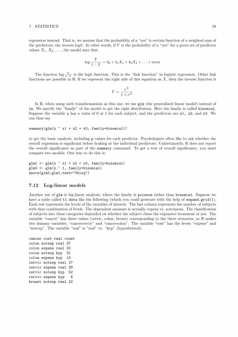
7 STATISTICS 58

regression instead. That is, we assume that the probability of a “yes” is certain function of a weighted sum ofthe predictors, the inverse logit. In other words, if Y is the probability of a “yes” for a given set of predictorvalues X1, X2, . . . , the model says that

logY

1− Y= b0 + b1X1 + b2X2 + . . . + error

The function log Y1−Y is the logit function. This is the “link function” in logistic regression. Other link

functions are possible in R. If we represent the right side of this equation as X, then the inverse function is

Y =eX

1 + eX

In R, when using such transformations as this one, we use glm (the generalized linear model) instead oflm. We specify the “family” of the model to get the right distribution. Here the family is called binomial.Suppose the variable y has a value of 0 or 1 for each subject, and the predictors are x1, x2, and x3. Wecan thus say

summary(glm(y ~ x1 + x2 + x3, family=binomial))

to get the basic analysis, including p values for each predictor. Psychologists often like to ask whether theoverall regression is significant before looking at the individual predictors. Unfortunately, R does not reportthe overall significance as part of the summary command. To get a test of overall significance, you mustcompare two models. One way to do this is:

glm1 <- glm(y ~ x1 + x2 + x3, family=binomial)glm0 <- glm(y ~ 1, family=binomial)anova(glm0,glm1,test="Chisq")

7.12 Log-linear models

Another use of glm is log-linear analysis, where the family is poisson rather than binomial. Suppose wehave a table called t1.data like the following (which you could generate with the help of expand.grid()).Each row represents the levels of the variables of interest. The last column represents the number of subjectswith that combination of levels. The dependent measure is actually expens vs. notexpens. The classificationof subjects into these categories depended on whether the subject chose the expensive treatment or not. Thevariable “cancer” has three values (cervic, colon, breast) corresponding to the three scenarios, so R makestwo dummy variables, “cancercervic” and “cancercolon”. The variable “cost” has the levels “expens” and“notexp”. The variable “real” is ”real” vs. “hyp” (hypothetical).

cancer cost real countcolon notexp real 37colon expens real 20colon notexp hyp 31colon expens hyp 15cervic notexp real 27cervic expens real 28cervic notexp hyp 52cervic expens hyp 6breast notexp real 22

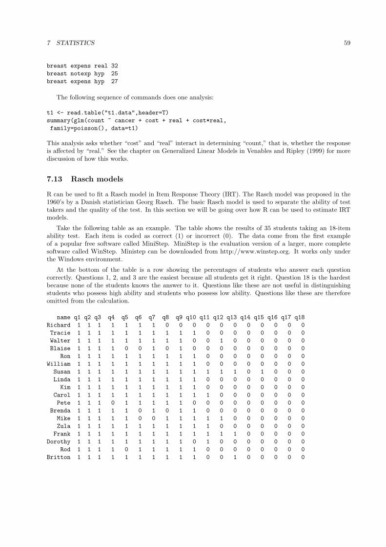
7 STATISTICS 59

breast expens real 32breast notexp hyp 25breast expens hyp 27

The following sequence of commands does one analysis:

t1 <- read.table("t1.data",header=T)summary(glm(count ~ cancer + cost + real + cost*real,family=poisson(), data=t1)

This analysis asks whether “cost” and “real” interact in determining “count,” that is, whether the responseis affected by “real.” See the chapter on Generalized Linear Models in Venables and Ripley (1999) for morediscussion of how this works.

7.13 Rasch models

R can be used to fit a Rasch model in Item Response Theory (IRT). The Rasch model was proposed in the1960’s by a Danish statistician Georg Rasch. The basic Rasch model is used to separate the ability of testtakers and the quality of the test. In this section we will be going over how R can be used to estimate IRTmodels.

Take the following table as an example. The table shows the results of 35 students taking an 18-itemability test. Each item is coded as correct (1) or incorrect (0). The data come from the first exampleof a popular free software called MiniStep. MiniStep is the evaluation version of a larger, more completesoftware called WinStep. Ministep can be downloaded from http://www.winstep.org. It works only underthe Windows environment.

At the bottom of the table is a row showing the percentages of students who answer each questioncorrectly. Questions 1, 2, and 3 are the easiest because all students get it right. Question 18 is the hardestbecause none of the students knows the answer to it. Questions like these are not useful in distinguishingstudents who possess high ability and students who possess low ability. Questions like these are thereforeomitted from the calculation.

name q1 q2 q3 q4 q5 q6 q7 q8 q9 q10 q11 q12 q13 q14 q15 q16 q17 q18Richard 1 1 1 1 1 1 1 0 0 0 0 0 0 0 0 0 0 0Tracie 1 1 1 1 1 1 1 1 1 1 0 0 0 0 0 0 0 0Walter 1 1 1 1 1 1 1 1 1 0 0 1 0 0 0 0 0 0Blaise 1 1 1 1 0 0 1 0 1 0 0 0 0 0 0 0 0 0

Ron 1 1 1 1 1 1 1 1 1 1 0 0 0 0 0 0 0 0William 1 1 1 1 1 1 1 1 1 1 0 0 0 0 0 0 0 0

Susan 1 1 1 1 1 1 1 1 1 1 1 1 1 0 1 0 0 0Linda 1 1 1 1 1 1 1 1 1 1 0 0 0 0 0 0 0 0

Kim 1 1 1 1 1 1 1 1 1 1 0 0 0 0 0 0 0 0Carol 1 1 1 1 1 1 1 1 1 1 1 0 0 0 0 0 0 0Pete 1 1 1 0 1 1 1 1 1 0 0 0 0 0 0 0 0 0

Brenda 1 1 1 1 1 0 1 0 1 1 0 0 0 0 0 0 0 0Mike 1 1 1 1 1 0 0 1 1 1 1 1 0 0 0 0 0 0Zula 1 1 1 1 1 1 1 1 1 1 1 0 0 0 0 0 0 0

Frank 1 1 1 1 1 1 1 1 1 1 1 1 1 0 0 0 0 0Dorothy 1 1 1 1 1 1 1 1 1 0 1 0 0 0 0 0 0 0

Rod 1 1 1 1 0 1 1 1 1 1 0 0 0 0 0 0 0 0Britton 1 1 1 1 1 1 1 1 1 1 0 0 1 0 0 0 0 0

7 STATISTICS 60

Janet 1 1 1 1 1 1 1 1 1 0 0 0 0 0 0 0 0 0David 1 1 1 1 1 1 1 1 1 1 0 0 1 0 0 0 0 0

Thomas 1 1 1 1 1 1 1 1 1 1 1 0 1 0 0 0 0 0Betty 1 1 1 1 1 1 1 1 1 1 1 1 0 0 0 0 0 0Bert 1 1 1 1 1 1 1 1 1 1 0 0 1 1 0 0 0 0Rick 1 1 1 1 1 1 1 1 1 1 1 0 1 0 0 1 1 0Don 1 1 1 0 1 1 0 0 0 0 0 0 0 0 0 0 0 0

Barbara 1 1 1 1 1 1 1 1 1 1 0 0 0 0 0 0 0 0Adam 1 1 1 1 1 1 1 0 0 0 0 0 0 0 0 0 0 0

Audrey 1 1 1 1 1 1 1 1 1 0 1 0 0 0 0 0 0 0Anne 1 1 1 1 1 1 0 0 1 1 1 0 0 1 0 0 0 0Lisa 1 1 1 1 1 1 1 1 1 0 0 0 0 0 0 0 0 0

James 1 1 1 1 1 1 1 1 1 1 0 0 0 0 0 0 0 0Joe 1 1 1 1 1 1 1 1 1 1 1 0 0 0 0 0 0 0

Martha 1 1 1 1 0 0 1 0 0 1 0 0 0 0 0 0 0 0Elsie 1 1 1 1 1 1 1 1 1 1 0 1 0 1 0 0 0 0Helen 1 1 1 0 0 0 0 0 0 0 0 0 0 0 0 0 0 0

----------------------------------------------------------------------------1 1 1 .91 .88 .86 .88 .77 .86 .69 .34 .17 .20 .09 .03 .03 .03 0.0

We also need to examine if there are students who get all or none of the items right. If we omit items 1,2, 3, and 18, and we take a look at the the 0’s and 1’s for each student, then we see that Helen fails on allremaining items. Helen therefore tells us nothing about which item is harder and which is easier. All itemsare beyond Helen’s ability. Students who can get all items right also do not give us useful information. Butin this example none of the students can answer all items correctly.

This is how many specific-purpose statistical packages prepare the raw data for IRT analysis. Thesepackages set aside any items or persons that provide no useful information for the analysis. They analyzethe IRT model with the remaining data. From the solutions derived from the remaining data, these packagesextrapolate to come up with estimates for items and persons first set aside.

In R we can use a conditional logit model to perform IRT analyses. The conditinal logit model is inthe survival analysis library maintained by Thomas Lumley at University of Washington. A description ofthe survival analysis library and the additional packages it depends on can be obtained by the R commandlibrary(help=survival). The R codes offered in this section have been tested with version 2.11-4 of thesurvival library in R-1.9.0.

The original derivation by Rasch was different but equivalent to a fixed-effect conditional logit model.Note that the following procedures in R are suitable only for binary items (e.g., pass/fail on test items).

The Rasch model states that the log odds of a person s answering an item i correctly is a function ofthe person’s ability (θs) and the item’s difficulty (βi). Difficult items are hard to get right even for peoplewith high ability. The odds of getting an item right decreases with item difficulty (and thus the minus signbefore βi). The notations we use here are from Embretson and Reise (2000).

logit(pi,s) = log(Pr(pi,s)

Pr(1− pi,s)) = θs − βi,

wheres = 1, . . . , number of persons; i = 1, . . . , number of items; and θs ≈ Normal(0, τ).

The example data, after removing Helen and items 1, 2, 3, and 18, contain 34 students (s = 1, 2, . . . 34)and 17 items (i = i, 2, . . . 17). Richard is person 1, Tracie is person 2, ..., and so on. To evaluate Richard’schance of answering item 3 correctly, we take Richard’s abiliy (say, it is 3 in logit unit), substract it out with

7 STATISTICS 61

item 3’s difficulty (say, it is 2.2 in logit unit), and we get a 0.8 logit. We can convert the logit scale backto probability by taking exp(0.8)/(1 + exp(0.8)) and we get 0.69. Richard has a 69% chance of gettingitem 3 right.

The question is, how do we calculate the θ’s and the β’s in the equation?

We need to first load the survival analysis library by typing library(survival). Then we need to setaside uninformative items and persons. This is done by the following commands:

> library(survival)> exam1 <- read.csv(file="exam1.dat", sep="", header=T, row.names=NULL)> exam1$id <- factor(paste("s", 1:dim(exam1)[1], sep=""))> #> # percentage of Ss who can correctly answer the items> #> round(apply(exam1[, 3:20], 2, mean), 2) # items 1, 2, 3 and 18 are no good

q1 q2 q3 q4 q5 q6 q7 q8 q9 q10 q11 q12 q13 q14 q15 q161.00 1.00 1.00 0.91 0.89 0.86 0.89 0.77 0.86 0.69 0.34 0.17 0.20 0.09 0.03 0.03q17 q18

0.03 0.00> round(apply(exam1[, 7:19], 1, mean), 2) # Helen got every good item wrong

1 2 3 4 5 6 7 8 9 10 11 12 13 14 15 160.23 0.46 0.46 0.15 0.46 0.46 0.77 0.46 0.46 0.54 0.38 0.31 0.46 0.54 0.69 0.46

17 18 19 20 21 22 23 24 25 26 27 28 29 30 31 320.38 0.54 0.38 0.54 0.62 0.62 0.62 0.77 0.15 0.46 0.23 0.46 0.46 0.38 0.46 0.54

33 34 350.15 0.62 0.00> exam1[35, ]

name sex q1 q2 q3 q4 q5 q6 q7 q8 q9 q10 q11 q12 q13 q14 q15 q16 q17 q18 id35 Helen F 1 1 1 0 0 0 0 0 0 0 0 0 0 0 0 0 0 0 s35> # remove items 1, 2, 3, and 18 because they provide no useful information> names(exam1)[1] "name" "sex" "q1" "q2" "q3" "q4" "q5" "q6" "q7" "q8"

[11] "q9" "q10" "q11" "q12" "q13" "q14" "q15" "q16" "q17" "q18"[21] "id"> exam1.1 <- exam1[, -c(3,4,5,20)]> # remove Helen, who answered all good items incorrectly> exam1.1 <- exam1[ -dim(exam1)[1], ]

To run the conditional logit model clog(), we need to reshape the data from a wide format to a longformat. The reshape() command takes q4:q17 and organize them into a new variable called resp. Anothernew varible item is created to identify questions 4 to 17.

> exam1.1 <- reshape(exam1.1, varying=list(paste("q", 4:17, sep="")),+ timevar="item", v.names="resp", direction="long")

In the equation the item difficulty parameters (the β’s) have a minus sign before them. In clog() aparameter with a minus sign is represented by a dummy variable of -1. For example, in the long form theitems are identified by the variable item. An excerpt of the full data shows that Martha answered item 1correctly, Elsie also answered item 1 correctly. The answers of Martha and Elsie for item 1 are followed byanswers of Richard, Tracie, and Walter to the next item (item 2).

> exam1.1[34:38, ]

7 STATISTICS 62

name sex id item resps33.1 Martha F s33 1 1s34.1 Elsie F s34 1 1s1.2 Richard M s1 2 1s2.2 Tracie F s2 2 1s3.2 Walter M s3 2 1

Using the above data excerpt as an example, we can create dummy variables for items 1 and 2. TheR command is tt <- factor(exam1.1[34:38, "item"]); dummy <- diag(nlevels(tt))[tt, ] and youhave:

> cbind(exam1.1[34:38, ], 0 - dummy)name sex id item resp 1 2

s34.1 Elsie F s34 1 1 -1 0s35.1 Helen F s35 1 1 -1 0s1.2 Richard M s1 2 1 0 -1s2.2 Tracie F s2 2 1 0 -1s3.2 Walter M s3 2 1 0 -1

Note that the last two columns are added with cbind() and they can be used to code the β parametersfor items 1 and 2, respectively. When this is applied to the 476 rows in the data set, it produces a dummyvariable matrix of 476 rows and 14 columns. Each column of the matrix will be used to estimate the itemdifficulty associated with each of questions 4 to 17.

> ex.i.dummy <- diag(nlevels(factor(exam1.1$item)))[factor(exam1.1$item), ]> ex.i.dummy <- 0 - ex.i.dummy # turns (0, 1) into (0, -1)> ex.i.dummy <- data.frame(ex.i.dummy, row.names=NULL)> dimnames(ex.i.dummy)[[2]] <- paste("i", 4:17, sep="")> dim(ex.i.dummy)[1] 476 14

Finally, a call to clogit() completes the calculations. Worth noting is how the syntax is written. Thestrata() function tells clogit() to estimate item difficulty associated with each dummy variable by holdingconstant the influence across different persons. The syntax also specifies that the item difficulty paramatersbe estimated for all items except i4. This is because i4 is the reference level when all dummy variables arezero. The clogit() function is not able to define a reference level if i4 is added. The clogit() functionwith i4 does not know what to do when all dummy variables are zero.

> attach(ex.i.dummy) # attach the dummy variables so I can call i4:i17> # item 4 is the reference> exam2.clog<- clogit(resp ~ i5+i6+i7+i8+i9+i10+i11+i12+i13+i14++ i15+i16+i17+ strata(id), data=exam1.1)> summary(exam2.clog)Call:clogit(resp ~ i5 + i6 + i7 + i8 + i9 + i10 + i11 + i12 + i13 +

i14 + i15 + i16 + i17 + strata(id), data = exam1.1)

n= 476

coef exp(coef) se(coef) z pi5 0.514 1.67 1.025 0.501 6.2e-01

7 STATISTICS 63

i6 0.923 2.52 0.991 0.931 3.5e-01i7 0.514 1.67 1.025 0.501 6.2e-01i8 1.875 6.52 0.955 1.964 5.0e-02i9 0.923 2.52 0.991 0.931 3.5e-01i10 2.598 13.44 0.944 2.752 5.9e-03i11 4.517 91.54 0.954 4.736 2.2e-06i12 5.792 327.53 1.028 5.632 1.8e-08i13 5.537 253.95 1.010 5.484 4.1e-08i14 6.825 920.74 1.136 6.007 1.9e-09i15 8.095 3278.95 1.403 5.772 7.8e-09i16 8.095 3278.95 1.403 5.772 7.8e-09i17 8.095 3278.95 1.403 5.772 7.8e-09

exp(coef) exp(-coef) lower .95 upper .95i5 1.67 0.597954 0.224 12.5i6 2.52 0.397477 0.361 17.6i7 1.67 0.597954 0.224 12.5i8 6.52 0.153373 1.004 42.4i9 2.52 0.397477 0.361 17.6i10 13.44 0.074425 2.112 85.5i11 91.54 0.010924 14.120 593.5i12 327.53 0.003053 43.650 2457.7i13 253.95 0.003938 35.104 1837.0i14 920.74 0.001086 99.293 8538.0i15 3278.95 0.000305 209.826 51240.2i16 3278.95 0.000305 209.826 51240.2i17 3278.95 0.000305 209.826 51240.2

Rsquare= 0.525 (max possible= 0.659 )Likelihood ratio test= 355 on 13 df, p=0Wald test = 108 on 13 df, p=0Score (logrank) test = 277 on 13 df, p=0

With the i4 being the reference level, the coeffiencts associated with the dummy variables should beinterpreted as the differences in item difficulty between i4 and each of i5 to i17. For example, the 0.514associated with i5 means that i5 is more difficult (remember, higher β means higher difficulty) than i4 by0.514. In addition, items 15, 16, and 17 are equally difficult. They are more difficult than i4 by 8.095 logits.This translates to a reduction in the probability of answering items 15, 16, and 17 correctly. On a probabilityscale, this 8.095 logit is equivalent to 0.999 reduction in probability (try exp(8.095) / ( 1 + exp(8.095))).

The clogit() function in R is general-purpose routine designed for fitting a conditional logit model.Thus it does not automatically print out many other statistics specific to Rasch model. For example, thesummary() function does not automatically generate the estimated ability level for each person. Otherpackages like MiniStep does that for you. But clogit() in R provides estimates of item difficulty, which arethe most important information for developing surveys or tests.

7.14 Conjoint analysis

In true conjoint analysis, we present a subject with stimuli made by crossing at least two different variables.For example, in one study, Baron and Andrea Gurmankin presented each subject with 56 items in a randomorder. The items consisted of each of each of eight medical conditions (ranging from a wart to immediate

7 STATISTICS 64

death) at each of seven probability levels, and the subjects provided a badness rating for each of the 56items. The assumption of conjoint analysis is that the subject behaves as if he represents the disutility ofeach condition as a number, and the probability as another number, adds the two numbers, and transformsthe result monotonically into the response scale provided. The representation of probability is a monotonicfunction of the given probability.

When we analyze the data, we try to recover the three transformations so as to get the best fit assumingthat this model is true. The three transformations are the assignment of numbers to the probabilities, theassignment of numbers to the conditions, and the function relating the result to the response scale. (In thiscase, if the subject followed expected-utility theory, the probability would be transformed logarithmically,so that the additive representation corresponded to multiplication.)

R does not have a conjoint analysis package as such. But the Acepack package contains a functioncalled ace(), for “alternating conditional expectations,” which does essentially what we want. It maximizesthe variance in the dependent variable (the response) that is explained by the predictors (probability andcondition), by using an iterative process. Here is an example in which the response is called bad, which isa matrix in which the rows are subjects, and within each row the probabilities are in groups of 8, with theconditions repeated in each group.

probs <- rep(1:7,rep(8,7))conds <- gl(8,1,56)cnames <- c("wart","toe","deaf1","leg1","leg2","blind","bbdd","death")pnames <- c(".001",".0032",".01",".032",".1",".32","1")

c.wt.ace <- matrix(0,ns,8) # resulting numbers for conditionsp.wt.ace <- matrix(0,ns,7) # resulting transformed probabilitiesbad.ace <- matrix(0,ns,56) # transformed responses

for (i in 1:ns) # fit the model for each subject{av1 <- ace(cbind(probs,conds),bad[i,],lin=1)bad.ace[i,] <- av1$typ.wt.ace[i,] <- av1$tx[8*0:6+1,1]c.wt.ace[i,] <- av1$tx[1:8,2]

}

In the end, the matrices p.wt.ace, c.wt.ace and bad.ace should have the transformed numbers, onerow per subject.

7.15 Imputation of missing data

Schafer and Graham (2002) provide a good review of methods for dealing with missing data. R providesmany of the methods that they discuss. One method is multiple imputation, which is found in the Hmiscpackage. Each missing datum is inferred repeated from different samples of other variables, and the repeatedinferences are used to determine the error. It turns out that this method works best with the ols() functionfrom the Design package rather than with (the otherwise equivalent) lm() function. Here is an example,using the data set t1.

library(Hmisc)f <- aregImpute(~v1+v2+v3+v4, n.impute=20,

fweighted=.2, defaultLinear=T, data=t1)library(Design)

8 REFERENCES 65

fmp <- fit.mult.impute(v1~v2+v3, ols, f, data=t1)summary(fmp)

The first command (f) imputes missing values in all four variables, using the other three for each variable.The second command (fmp) estimates a regression model in which v1 is predicted from two of the remainingvariables. A variable can be used (and should be used, if it is useful) for imputation even when it is not usedin the model.

8 References

Chambers, J. M., & Hastie, T. J. (1992). Statistical models in S. Pacific Grove, CA: Wadsworth & BrooksCole Advanced Books and Software.

Clark, H. H. (1973). The language-as-fixed-effect fallacy: A critique of language statistics in psychologicalresearch. Journal of Verbal Learning & Verbal Behavior, 12, 335–359.

Hays, W. L. (1988, 4th ed.) Statistics. New York: Holt, Rinehart and Winston.

Hoaglin, D. C., Mosteller, F., & Tukey, J. W. (Eds.) (1983). Understanding robust and exploratory dataanalysis. New York: Wiley.

Lord, F. M., & Novick, M. R. (1968). Statistical theories of mental test scores. Reading, MA: Addison-Wesley.

Maxwell, S. E. & Delaney, H. D. (1990) Designing Experiments and Analyzing Data: A model comparisonperspective. Pacific Grove, CA: Brooks/Cole.

Schafer, J. L., & Graham, J. W. (2002). Missing data: Our view of the state of the art. PsychologicalMethods, 7, 147–177.

Stevens, J. (1992, 2nd ed) Applied Multivariate Statistics for the Social Sciences. Hillsdale, NJ: Erlbaum.

Venables, W. N., & Ripley, B. D. (1999). Modern applied statistics with S–PLUS (3rd Ed.). New York:Springer.

Notes on the use of R for psychology experiments and ...

Documents

Transcript of Notes on the use of R for psychology experiments and ...