NOTES AND CORRESPONDENCE Dynamical Mechanisms …faculty.nps.edu/pcchu/web_paper/jpo/edmons.pdf ·...

NOVEMBER 1999 2971N O T E S A N D C O R R E S P O N D E N C E

NOTES AND CORRESPONDENCE

Dynamical Mechanisms for the South China Sea Seasonal Circulation andThermohaline Variabilities

PETER C. CHU, NATHAN L. EDMONS, AND CHENWU FAN

Department of Oceanography, Naval Postgraduate School, Monterey, California

14 July 1998 and 8 April 1999

ABSTRACT

The seasonal ocean circulation and the seasonal thermal structure in the South China Sea (SCS) were studiednumerically using the Princeton Ocean Model (POM) with 20-km horizontal resolution and 23 sigma levelsconforming to a realistic bottom topography. A 16-month control run was performed using climatological monthlymean wind stresses, restoring-type surface salt and heat, and observational oceanic inflow/outflow at the openboundaries. The seasonally averaged effects of isolated forcing terms are presented and analyzed from thefollowing experiments: 1) nonlinear dynamic effects removed, 2) wind effects removed, and 3) open boundaryinflow/outflow set to zero. This procedure allowed analysis of the contribution of individual parameters to thegeneral hydrology and specific features of the SCS: for example, coastal jets, mesoscale topographic gyres, andcountercurrents. The results show that the POM model has the capability of simulating seasonal variations ofthe SCS circulation and thermohaline structure. The simulated SCS surface circulation is generally anticyclonic(cyclonic) during the summer (winter) monsoon period with a strong western boundary current, a mean maximumspeed of 0.5 m s21 (0.95 m s21), a mean volume transport of 5.5 Sv (10.6 Sv) (Sv [ 106 m3 s21), and extendingto a depth of around 200 m (500 m). During summer, the western boundary current splits and partially leavesthe coast; the bifurcation point is at 148N in May and shifts south to 108N in July. A mesoscale eddy on theSunda shelf (Natuna Island eddy) was also simulated. This eddy is cyclonic (anticyclonic) with maximum swirlvelocity of 0.6 m s21 at the peak of the winter (summer) monsoon. The simulated thermohaline structure forsummer and winter are nearly horizontal from east to west except at the coastal regions. Coastal upwelling anddownwelling are also simulated: localized lifting (descending) of the isotherms and isohalines during summer(winter) at the west boundary. The simulation is reasonable when compared to the observations. Sensitivityexperiments were designed to investigate the driving mechanisms. Nonlinearity is shown to be important to thetransport of baroclinic eddy features, but otherwise insignificant. Transport from lateral boundaries is of con-siderable importance to summer circulation and thermal structure, with lesser effect on winter monsoon hydrology.In general, seasonal circulation patterns and upwelling phenomena are determined and forced by the wind, whilethe lateral boundary forcing plays a secondary role in determining the magnitude of the circulation velocities.

1. Introduction

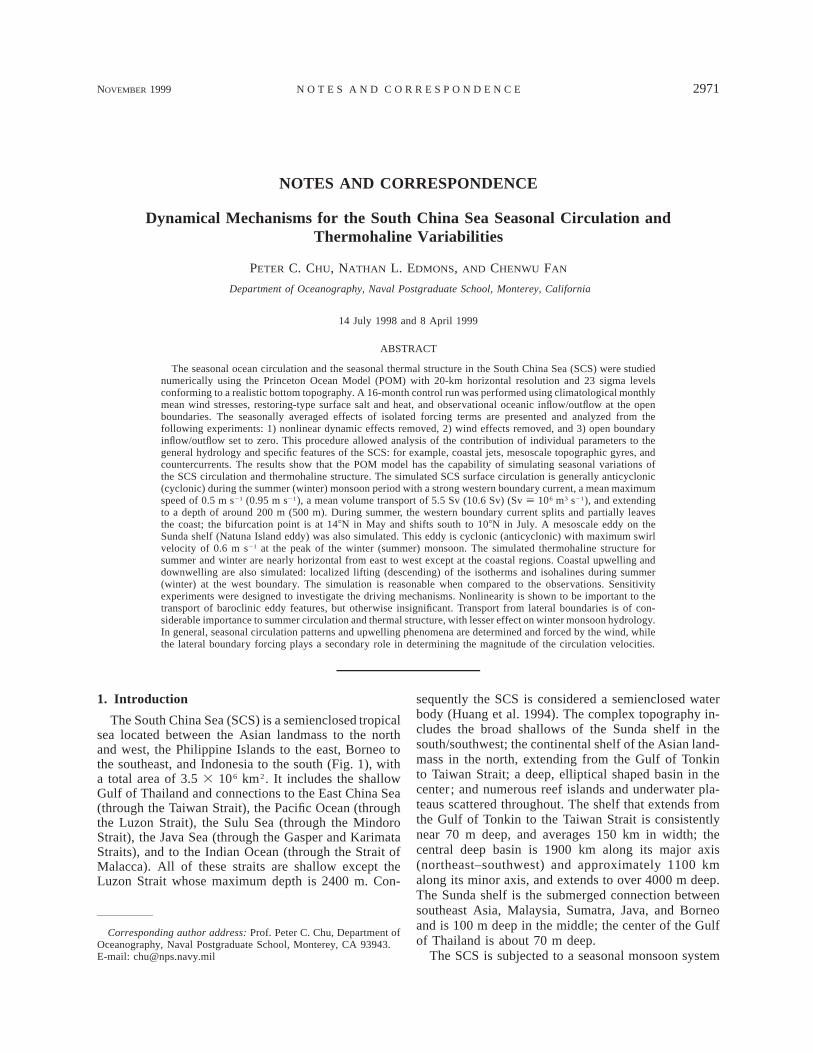
The South China Sea (SCS) is a semienclosed tropicalsea located between the Asian landmass to the northand west, the Philippine Islands to the east, Borneo tothe southeast, and Indonesia to the south (Fig. 1), witha total area of 3.5 3 106 km2. It includes the shallowGulf of Thailand and connections to the East China Sea(through the Taiwan Strait), the Pacific Ocean (throughthe Luzon Strait), the Sulu Sea (through the MindoroStrait), the Java Sea (through the Gasper and KarimataStraits), and to the Indian Ocean (through the Strait ofMalacca). All of these straits are shallow except theLuzon Strait whose maximum depth is 2400 m. Con-

Corresponding author address: Prof. Peter C. Chu, Department ofOceanography, Naval Postgraduate School, Monterey, CA 93943.E-mail: [email protected]

sequently the SCS is considered a semienclosed waterbody (Huang et al. 1994). The complex topography in-cludes the broad shallows of the Sunda shelf in thesouth/southwest; the continental shelf of the Asian land-mass in the north, extending from the Gulf of Tonkinto Taiwan Strait; a deep, elliptical shaped basin in thecenter; and numerous reef islands and underwater pla-teaus scattered throughout. The shelf that extends fromthe Gulf of Tonkin to the Taiwan Strait is consistentlynear 70 m deep, and averages 150 km in width; thecentral deep basin is 1900 km along its major axis(northeast–southwest) and approximately 1100 kmalong its minor axis, and extends to over 4000 m deep.The Sunda shelf is the submerged connection betweensoutheast Asia, Malaysia, Sumatra, Java, and Borneoand is 100 m deep in the middle; the center of the Gulfof Thailand is about 70 m deep.

The SCS is subjected to a seasonal monsoon system

2972 VOLUME 29J O U R N A L O F P H Y S I C A L O C E A N O G R A P H Y

FIG. 1. Geography and isobaths showing the bathymetry (m) of the South China Sea.

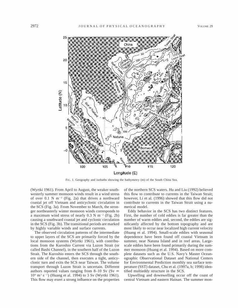
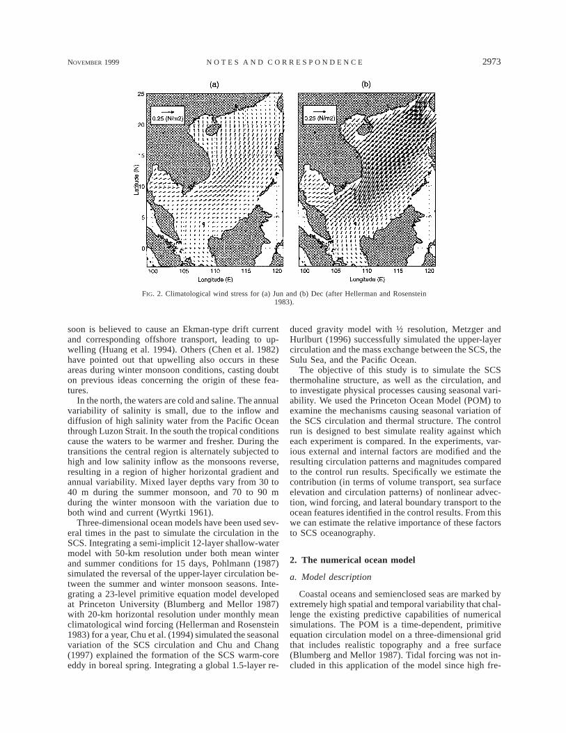
(Wyrtki 1961). From April to August, the weaker south-westerly summer monsoon winds result in a wind stressof over 0.1 N m22 (Fig. 2a) that drives a northwardcoastal jet off Vietnam and anticyclonic circulation inthe SCS (Fig. 3a). From November to March, the stron-ger northeasterly winter monsoon winds corresponds toa maximum wind stress of nearly 0.3 N m22 (Fig. 2b)causing a southward coastal jet and cyclonic circulationin the SCS (Fig. 3b). The transitional periods are markedby highly variable winds and surface currents.

The observed circulation patterns of the intermediateto upper layers of the SCS are primarily forced by thelocal monsoon systems (Wyrtki 1961), with contribu-tions from the Kuroshio Current via Luzon Strait (orcalled Bashi Channel), in the southern half of the LuzonStrait. The Kuroshio enters the SCS through the south-ern side of the channel, then executes a tight, anticy-clonic turn and exits the SCS near Taiwan. The volumetransport through Luzon Strait is uncertain. Differentauthors reported values ranging from 8–10 Sv (Sv [106 m3 s21) (Huang et al. 1994) to 3 Sv (Wyrtki 1961).This flow may exert a strong influence on the properties

of the northern SCS waters. Hu and Liu (1992) believedthis flow to contribute to currents in the Taiwan Strait;however, Li et al. (1996) showed that this flow did notcontribute to currents in the Taiwan Strait using a nu-merical model.

Eddy behavior in the SCS has two distinct features.First, the number of cold eddies is far greater than thenumber of warm eddies and, second, the eddies are sig-nificantly affected by the bottom topography and aremost likely to occur near localized high current velocity(Huang et al. 1994). Small-scale eddies with seasonaldependence have been found off coastal Vietnam insummer, near Natuna Island and in reef areas. Large-scale eddies have been found primarily during the sum-mer monsoon (Huang et al. 1994). Based on more com-plete datasets such as the U.S. Navy’s Master Ocean-ographic Observational Dataset and National Centersfor Environmental Prediction monthly sea surface tem-perature (SST) dataset, Chu et al. (1997a, b; 1998) iden-tified multieddy structure in the SCS.

Upwelling and downwelling occur off the coast ofcentral Vietnam and eastern Hainan. The summer mon-


FIG. 2. Climatological wind stress for (a) Jun and (b) Dec (after Hellerman and Rosenstein1983).

soon is believed to cause an Ekman-type drift currentand corresponding offshore transport, leading to up-welling (Huang et al. 1994). Others (Chen et al. 1982)have pointed out that upwelling also occurs in theseareas during winter monsoon conditions, casting doubton previous ideas concerning the origin of these fea-tures.

In the north, the waters are cold and saline. The annualvariability of salinity is small, due to the inflow anddiffusion of high salinity water from the Pacific Oceanthrough Luzon Strait. In the south the tropical conditionscause the waters to be warmer and fresher. During thetransitions the central region is alternately subjected tohigh and low salinity inflow as the monsoons reverse,resulting in a region of higher horizontal gradient andannual variability. Mixed layer depths vary from 30 to40 m during the summer monsoon, and 70 to 90 mduring the winter monsoon with the variation due toboth wind and current (Wyrtki 1961).

Three-dimensional ocean models have been used sev-eral times in the past to simulate the circulation in theSCS. Integrating a semi-implicit 12-layer shallow-watermodel with 50-km resolution under both mean winterand summer conditions for 15 days, Pohlmann (1987)simulated the reversal of the upper-layer circulation be-tween the summer and winter monsoon seasons. Inte-grating a 23-level primitive equation model developedat Princeton University (Blumberg and Mellor 1987)with 20-km horizontal resolution under monthly meanclimatological wind forcing (Hellerman and Rosenstein1983) for a year, Chu et al. (1994) simulated the seasonalvariation of the SCS circulation and Chu and Chang(1997) explained the formation of the SCS warm-coreeddy in boreal spring. Integrating a global 1.5-layer re-

duced gravity model with ½ resolution, Metzger andHurlburt (1996) successfully simulated the upper-layercirculation and the mass exchange between the SCS, theSulu Sea, and the Pacific Ocean.

The objective of this study is to simulate the SCSthermohaline structure, as well as the circulation, andto investigate physical processes causing seasonal vari-ability. We used the Princeton Ocean Model (POM) toexamine the mechanisms causing seasonal variation ofthe SCS circulation and thermal structure. The controlrun is designed to best simulate reality against whicheach experiment is compared. In the experiments, var-ious external and internal factors are modified and theresulting circulation patterns and magnitudes comparedto the control run results. Specifically we estimate thecontribution (in terms of volume transport, sea surfaceelevation and circulation patterns) of nonlinear advec-tion, wind forcing, and lateral boundary transport to theocean features identified in the control results. From thiswe can estimate the relative importance of these factorsto SCS oceanography.

2. The numerical ocean model

a. Model description

Coastal oceans and semienclosed seas are marked byextremely high spatial and temporal variability that chal-lenge the existing predictive capabilities of numericalsimulations. The POM is a time-dependent, primitiveequation circulation model on a three-dimensional gridthat includes realistic topography and a free surface(Blumberg and Mellor 1987). Tidal forcing was not in-cluded in this application of the model since high fre-


FIG. 3. Observational surface circulation: (a) Jun and (b) Dec (after Wyrtki 1961).


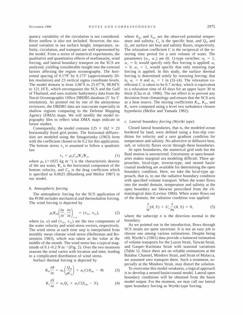
quency variability of the circulation is not considered.River outflow is also not included. However, the sea-sonal variation in sea surface height, temperature, sa-linity, circulation, and transport are well represented bythe model. From a series of numerical experiments, thequalitative and quantitative effects of nonlinearity, windforcing, and lateral boundary transport on the SCS areanalyzed, yielding considerable insight into the externalfactors affecting the region oceanography. The hori-zontal spacing of 0.1798 by 0.1758 (approximately 20-km resolution) and 23 vertical sigma coordinate levels.The model domain is from 3.068S to 25.078N, 98.848Eto 121.168E, which encompasses the SCS and the Gulfof Thailand, and uses realistic bathymetry data from theNaval Oceanographic Office DBDB5 database (59 by 59resolution). As pointed out by one of the anonymousreviewers, the DBDB5 data are inaccurate especially inshallow regions comparing to the Defense MappingAgency (DMA) maps. We will modify the model to-pography files to reflect what DMA maps indicate infuture studies.

Consequently, the model contains 125 3 162 3 23horizontally fixed grid points. The horizontal diffusiv-ities are modeled using the Smagorinsky (1963) formwith the coefficient chosen to be 0.2 for this application.The bottom stress t b is assumed to follow a quadraticlaw

t b 5 r0CD|Vb|Vb, (1)

where r0 (51025 kg m23) is the characteristic densityof the sea water, Vb is the horizontal component of thebottom velocity, and CD is the drag coefficient whichis specified as 0.0025 (Blumberg and Mellor 1987) inour model.

b. Atmospheric forcing

The atmospheric forcing for the SCS application ofthe POM includes mechanical and thermohaline forcing.The wind forcing is depicted by

]u ]yr K , 5 (t , t ), (2)0 M 0x 0y1 2]z ]z

z50

where (u, y) and (t 0x, t 0y) are the two components ofthe water velocity and wind stress vectors, respectively.The wind stress at each time step is interpolated frommonthly mean climate wind stress (Hellerman and Ro-senstein 1983), which was taken as the value at themiddle of the month. The wind stress has a typical mag-nitude of 0.1–0.2 N m22 (Fig. 2). Over the two monsoonseasons the wind varies with location and time, leadingto a complicated distribution of wind stress.

Surface thermal forcing is depicted by

]u QHK 5 a 1 a C(u 2 u) (3)H 1 2 obs1 2]z rCp

]SK 5 a Q 1 a C(S 2 S ), (4)S 1 S 2 obs]z

where uobs and Sobs are the observed potential temper-ature and salinity, Cp is the specific heat, and QH andQS are surface net heat and salinity fluxes, respectively.The relaxation coefficient C is the reciprocal of the re-storing time period for a unit volume of water. Theparameters (a1, a2) are (0, 1)-type switches: a1 5 1,a2 5 0, would specify only flux forcing is applied; a1

5 0, a2 5 1, would specify that only restoring typeforcing is applied. In this study, the surface thermalforcing is determined solely by restoring forcing; thatis, a1 5 0 and a2 5 1 in (3)–(4). The relaxation co-efficient C is taken to be 0.7 m/day, which is equivalentto a relaxation time of 43 days for an upper layer 30 mthick (Chu et al. 1996). The net effect is to prevent anydeviation from climatology and ensure that the SCS actsas a heat source. The mixing coefficients KM, KH, andKS were computed using a level two turbulence closurehypothesis (Mellor and Yamada 1982).

c. Lateral boundary forcing (Wyrtki type)

Closed lateral boundaries, that is, the modeled oceanbordered by land, were defined using a free-slip con-dition for velocity and a zero gradient condition fortemperature and salinity. No advective or diffusive heat,salt, or velocity fluxes occur through these boundaries.

At open boundaries, the numerical grid ends but thefluid motion is unrestricted. Uncertainty at open bound-aries makes marginal sea modeling difficult. Three ap-proaches, local-type, inverse-type, and nested basin/coastal modeling are available for determining the openboundary condition. Here, we take the local-type ap-proach, that is, to use the radiative boundary conditionwith specified volume transport. When the water flowsinto the model domain, temperature and salinity at theopen boundary are likewise prescribed from the cli-matological data (Levitus 1984). When water flows outof the domain, the radiation condition was applied:

] ](u, S ) 1 U (u, S ) 5 0, (5)n]t ]n

where the subscript n is the direction normal to theboundary.

As we pointed out in the introduction, flows throughSCS straits are quite uncertain. It is not an easy job tochoose one among various estimations. Despite beingold, Wyrtki’s (1961) data provide a balanced estimationof volume transports for the Luzon Strait, Taiwan Strait,and Gasper–Karimata Strait with seasonal variations(Table 1). Since there are no reliable estimations at theBalabac Channel, Mindoro Strait, and Strait of Malacca,we assumed zero transport there. Such a treatment, es-pecially at the Mindoro Strait, may distort the solution.

To overcome this model weakness, a logical approachis to develop a nested basin/coastal model. Lateral openboundary conditions will be obtained from the basinmodel output. For the moment, we may call our lateralopen boundary forcing as Wyrtki-type forcing.


TABLE 1. Bimonthly variation of volume transport (Sv) at the lateralopen boundaries. The positive/negative values mean outflow/inflowand were taken from Wyrtki (1961).

Month

Feb Apr Jun Aug Oct Dec

Gaspar–KarimataStraits

Luzon StraitTaiwan Strait

4.423.520.9

0.00.00.0

24.03.01.0

23.02.50.5

1.020.620.4

4.323.420.9

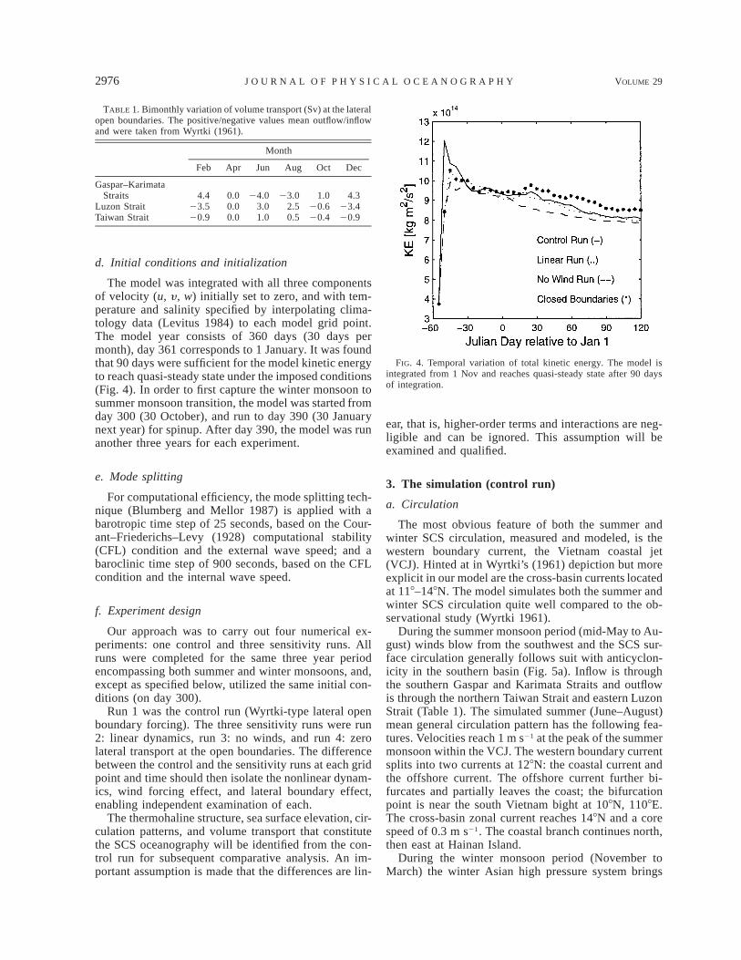
FIG. 4. Temporal variation of total kinetic energy. The model isintegrated from 1 Nov and reaches quasi-steady state after 90 daysof integration.

d. Initial conditions and initialization

The model was integrated with all three componentsof velocity (u, y , w) initially set to zero, and with tem-perature and salinity specified by interpolating clima-tology data (Levitus 1984) to each model grid point.The model year consists of 360 days (30 days permonth), day 361 corresponds to 1 January. It was foundthat 90 days were sufficient for the model kinetic energyto reach quasi-steady state under the imposed conditions(Fig. 4). In order to first capture the winter monsoon tosummer monsoon transition, the model was started fromday 300 (30 October), and run to day 390 (30 Januarynext year) for spinup. After day 390, the model was runanother three years for each experiment.

e. Mode splitting

For computational efficiency, the mode splitting tech-nique (Blumberg and Mellor 1987) is applied with abarotropic time step of 25 seconds, based on the Cour-ant–Friederichs–Levy (1928) computational stability(CFL) condition and the external wave speed; and abaroclinic time step of 900 seconds, based on the CFLcondition and the internal wave speed.

f. Experiment design

Our approach was to carry out four numerical ex-periments: one control and three sensitivity runs. Allruns were completed for the same three year periodencompassing both summer and winter monsoons, and,except as specified below, utilized the same initial con-ditions (on day 300).

Run 1 was the control run (Wyrtki-type lateral openboundary forcing). The three sensitivity runs were run2: linear dynamics, run 3: no winds, and run 4: zerolateral transport at the open boundaries. The differencebetween the control and the sensitivity runs at each gridpoint and time should then isolate the nonlinear dynam-ics, wind forcing effect, and lateral boundary effect,enabling independent examination of each.

The thermohaline structure, sea surface elevation, cir-culation patterns, and volume transport that constitutethe SCS oceanography will be identified from the con-trol run for subsequent comparative analysis. An im-portant assumption is made that the differences are lin-

ear, that is, higher-order terms and interactions are neg-ligible and can be ignored. This assumption will beexamined and qualified.

3. The simulation (control run)

a. Circulation

The most obvious feature of both the summer andwinter SCS circulation, measured and modeled, is thewestern boundary current, the Vietnam coastal jet(VCJ). Hinted at in Wyrtki’s (1961) depiction but moreexplicit in our model are the cross-basin currents locatedat 118–148N. The model simulates both the summer andwinter SCS circulation quite well compared to the ob-servational study (Wyrtki 1961).

During the summer monsoon period (mid-May to Au-gust) winds blow from the southwest and the SCS sur-face circulation generally follows suit with anticyclon-icity in the southern basin (Fig. 5a). Inflow is throughthe southern Gaspar and Karimata Straits and outflowis through the northern Taiwan Strait and eastern LuzonStrait (Table 1). The simulated summer (June–August)mean general circulation pattern has the following fea-tures. Velocities reach 1 m s21 at the peak of the summermonsoon within the VCJ. The western boundary currentsplits into two currents at 128N: the coastal current andthe offshore current. The offshore current further bi-furcates and partially leaves the coast; the bifurcationpoint is near the south Vietnam bight at 108N, 1108E.The cross-basin zonal current reaches 148N and a corespeed of 0.3 m s21. The coastal branch continues north,then east at Hainan Island.

During the winter monsoon period (November toMarch) the winter Asian high pressure system brings


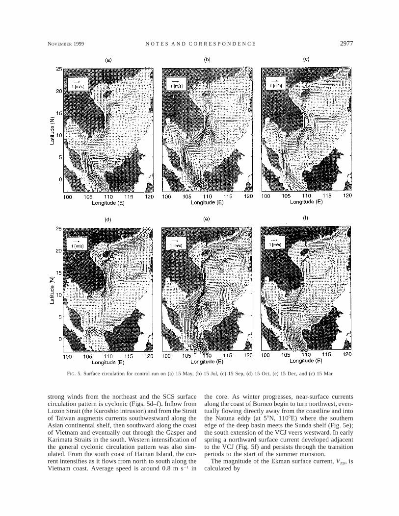
FIG. 5. Surface circulation for control run on (a) 15 May, (b) 15 Jul, (c) 15 Sep, (d) 15 Oct, (e) 15 Dec, and (c) 15 Mar.

strong winds from the northeast and the SCS surfacecirculation pattern is cyclonic (Figs. 5d–f). Inflow fromLuzon Strait (the Kuroshio intrusion) and from the Straitof Taiwan augments currents southwestward along theAsian continental shelf, then southward along the coastof Vietnam and eventually out through the Gasper andKarimata Straits in the south. Western intensification ofthe general cyclonic circulation pattern was also sim-ulated. From the south coast of Hainan Island, the cur-rent intensifies as it flows from north to south along theVietnam coast. Average speed is around 0.8 m s21 in

the core. As winter progresses, near-surface currentsalong the coast of Borneo begin to turn northwest, even-tually flowing directly away from the coastline and intothe Natuna eddy (at 58N, 1108E) where the southernedge of the deep basin meets the Sunda shelf (Fig. 5e);the south extension of the VCJ veers westward. In earlyspring a northward surface current developed adjacentto the VCJ (Fig. 5f) and persists through the transitionperiods to the start of the summer monsoon.

The magnitude of the Ekman surface current, VE0, iscalculated by


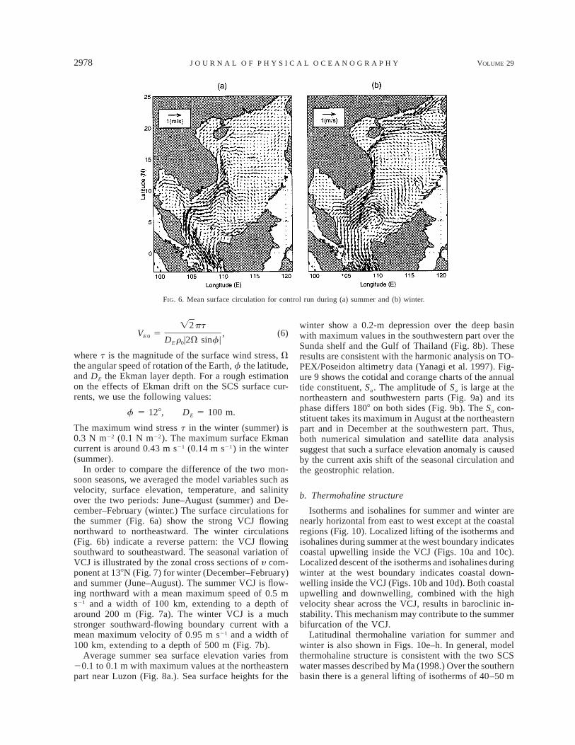
FIG. 6. Mean surface circulation for control run during (a) summer and (b) winter.

Ï2ptV 5 , (6)E0 D r |2V sinf |E 0

where t is the magnitude of the surface wind stress, Vthe angular speed of rotation of the Earth, f the latitude,and DE the Ekman layer depth. For a rough estimationon the effects of Ekman drift on the SCS surface cur-rents, we use the following values:

f 5 128, DE 5 100 m.

The maximum wind stress t in the winter (summer) is0.3 N m22 (0.1 N m22). The maximum surface Ekmancurrent is around 0.43 m s21 (0.14 m s21) in the winter(summer).

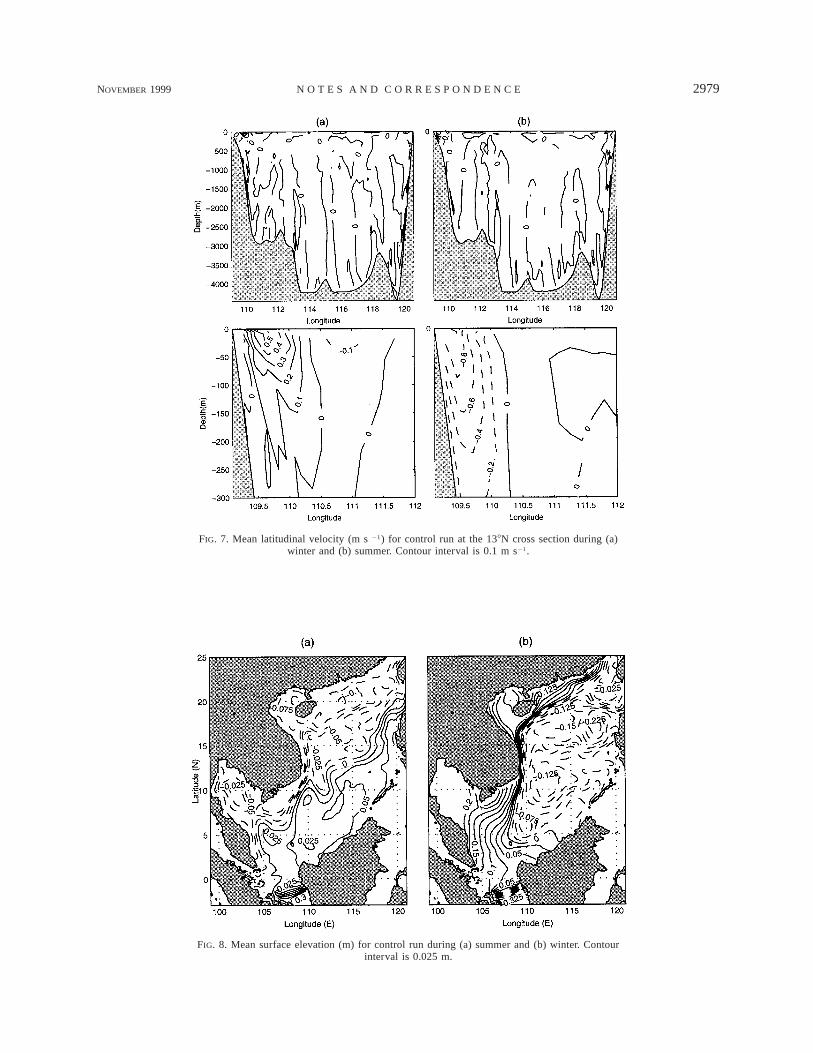
In order to compare the difference of the two mon-soon seasons, we averaged the model variables such asvelocity, surface elevation, temperature, and salinityover the two periods: June–August (summer) and De-cember–February (winter.) The surface circulations forthe summer (Fig. 6a) show the strong VCJ flowingnorthward to northeastward. The winter circulations(Fig. 6b) indicate a reverse pattern: the VCJ flowingsouthward to southeastward. The seasonal variation ofVCJ is illustrated by the zonal cross sections of y com-ponent at 138N (Fig. 7) for winter (December–February)and summer (June–August). The summer VCJ is flow-ing northward with a mean maximum speed of 0.5 ms21 and a width of 100 km, extending to a depth ofaround 200 m (Fig. 7a). The winter VCJ is a muchstronger southward-flowing boundary current with amean maximum velocity of 0.95 m s21 and a width of100 km, extending to a depth of 500 m (Fig. 7b).

Average summer sea surface elevation varies from20.1 to 0.1 m with maximum values at the northeasternpart near Luzon (Fig. 8a.). Sea surface heights for the

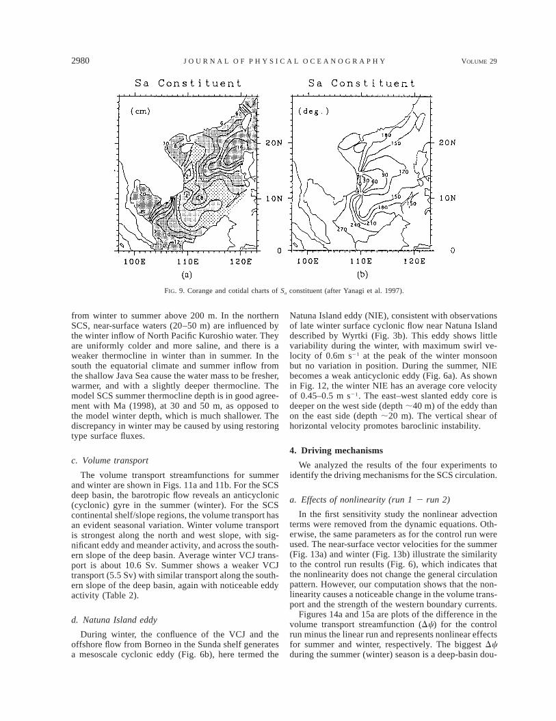
winter show a 0.2-m depression over the deep basinwith maximum values in the southwestern part over theSunda shelf and the Gulf of Thailand (Fig. 8b). Theseresults are consistent with the harmonic analysis on TO-PEX/Poseidon altimetry data (Yanagi et al. 1997). Fig-ure 9 shows the cotidal and corange charts of the annualtide constituent, Sa. The amplitude of Sa is large at thenortheastern and southwestern parts (Fig. 9a) and itsphase differs 1808 on both sides (Fig. 9b). The Sa con-stituent takes its maximum in August at the northeasternpart and in December at the southwestern part. Thus,both numerical simulation and satellite data analysissuggest that such a surface elevation anomaly is causedby the current axis shift of the seasonal circulation andthe geostrophic relation.

b. Thermohaline structure

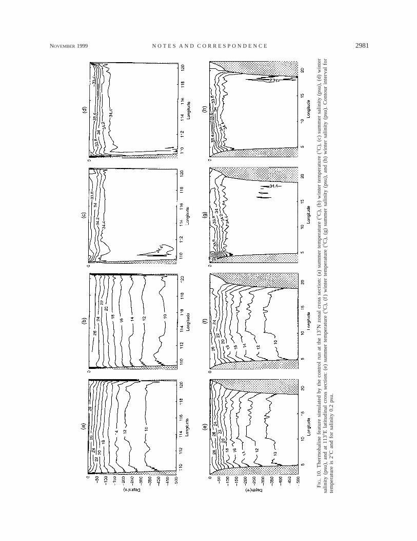
Isotherms and isohalines for summer and winter arenearly horizontal from east to west except at the coastalregions (Fig. 10). Localized lifting of the isotherms andisohalines during summer at the west boundary indicatescoastal upwelling inside the VCJ (Figs. 10a and 10c).Localized descent of the isotherms and isohalines duringwinter at the west boundary indicates coastal down-welling inside the VCJ (Figs. 10b and 10d). Both coastalupwelling and downwelling, combined with the highvelocity shear across the VCJ, results in baroclinic in-stability. This mechanism may contribute to the summerbifurcation of the VCJ.

Latitudinal thermohaline variation for summer andwinter is also shown in Figs. 10e–h. In general, modelthermohaline structure is consistent with the two SCSwater masses described by Ma (1998.) Over the southernbasin there is a general lifting of isotherms of 40–50 m


FIG. 7. Mean latitudinal velocity (m s 21) for control run at the 138N cross section during (a)winter and (b) summer. Contour interval is 0.1 m s21.

FIG. 8. Mean surface elevation (m) for control run during (a) summer and (b) winter. Contourinterval is 0.025 m.


FIG. 9. Corange and cotidal charts of Sa constituent (after Yanagi et al. 1997).

from winter to summer above 200 m. In the northernSCS, near-surface waters (20–50 m) are influenced bythe winter inflow of North Pacific Kuroshio water. Theyare uniformly colder and more saline, and there is aweaker thermocline in winter than in summer. In thesouth the equatorial climate and summer inflow fromthe shallow Java Sea cause the water mass to be fresher,warmer, and with a slightly deeper thermocline. Themodel SCS summer thermocline depth is in good agree-ment with Ma (1998), at 30 and 50 m, as opposed tothe model winter depth, which is much shallower. Thediscrepancy in winter may be caused by using restoringtype surface fluxes.

c. Volume transport

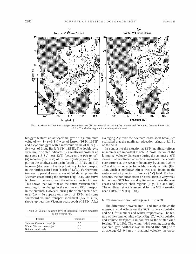
The volume transport streamfunctions for summerand winter are shown in Figs. 11a and 11b. For the SCSdeep basin, the barotropic flow reveals an anticyclonic(cyclonic) gyre in the summer (winter). For the SCScontinental shelf/slope regions, the volume transport hasan evident seasonal variation. Winter volume transportis strongest along the north and west slope, with sig-nificant eddy and meander activity, and across the south-ern slope of the deep basin. Average winter VCJ trans-port is about 10.6 Sv. Summer shows a weaker VCJtransport (5.5 Sv) with similar transport along the south-ern slope of the deep basin, again with noticeable eddyactivity (Table 2).

d. Natuna Island eddy

During winter, the confluence of the VCJ and theoffshore flow from Borneo in the Sunda shelf generatesa mesoscale cyclonic eddy (Fig. 6b), here termed the

Natuna Island eddy (NIE), consistent with observationsof late winter surface cyclonic flow near Natuna Islanddescribed by Wyrtki (Fig. 3b). This eddy shows littlevariability during the winter, with maximum swirl ve-locity of 0.6m s21 at the peak of the winter monsoonbut no variation in position. During the summer, NIEbecomes a weak anticyclonic eddy (Fig. 6a). As shownin Fig. 12, the winter NIE has an average core velocityof 0.45–0.5 m s21. The east–west slanted eddy core isdeeper on the west side (depth ;40 m) of the eddy thanon the east side (depth ;20 m). The vertical shear ofhorizontal velocity promotes baroclinic instability.

4. Driving mechanisms

We analyzed the results of the four experiments toidentify the driving mechanisms for the SCS circulation.

a. Effects of nonlinearity (run 1 2 run 2)

In the first sensitivity study the nonlinear advectionterms were removed from the dynamic equations. Oth-erwise, the same parameters as for the control run wereused. The near-surface vector velocities for the summer(Fig. 13a) and winter (Fig. 13b) illustrate the similarityto the control run results (Fig. 6), which indicates thatthe nonlinearity does not change the general circulationpattern. However, our computation shows that the non-linearity causes a noticeable change in the volume trans-port and the strength of the western boundary currents.

Figures 14a and 15a are plots of the difference in thevolume transport streamfunction (Dc) for the controlrun minus the linear run and represents nonlinear effectsfor summer and winter, respectively. The biggest Dcduring the summer (winter) season is a deep-basin dou-


FIG

.10

.T

herm

ohal

ine

feat

ure

sim

ulat

edby

the

cont

rol

run

atth

e13

8Nzo

nal

cros

sse

ctio

n:(a

)su

mm

erte

mpe

ratu

re(8

C),

(b)

win

ter

tem

pera

ture

(8C

),(c

)su

mm

ersa

lini

ty(p

su),

(d)

win

ter

sali

nity

(psu

),an

dat

1138

Ela

titu

dina

lcr

oss

sect

ion:

(e)

sum

mer

tem

pera

ture

(8C

),(f

)w

inte

rte

mpe

ratu

re(8

C),

(g)

sum

mer

sali

nity

(psu

),an

d(h

)w

inte

rsa

lini

ty(p

su).

Con

tour

inte

rval

for

tem

pera

ture

is28

Can

dfo

rsa

lini

ty0.

2ps

u.


FIG. 11. Mean total volume transport streamfunction (Sv) for control run during (a) summer and (b) winter. Contour interval is5 Sv. The shaded regions indicate negative values.

TABLE 2. Volume transport (Sv) of individual features simulatedby the control run.

Feature Transport

Summer Vietnam coastal jetWinter Vietnam coastal jetNatuna Island eddy

5.510.6

5.0

ble-gyre feature: an anticyclonic gyre with a minimumvalue of 24 Sv (26 Sv) west of Luzon (168N, 1168E)and a cyclonic gyre with a maximum value of 8 Sv (12Sv) west of Liyue Bank (118N, 1158E). The double-gyrestructure in winter indicates (i) a westward cross-basintransport (15 Sv) near 138N (between the two gyres),(ii) increase (decrease) of cyclonic (anticyclonic) trans-port in the southwestern basin (south of 138N), and (iii)increase (decrease) of anticyclonic (cyclonic) transportin the northeastern basin (north of 138N). Furthermore,two nearly parallel zero curves of Dc show up near theVietnam coast during the summer (Fig. 14a). One curveis close to the coast, and the other curve is offshore.This shows that Dc 5 0 on the entire Vietnam shelf,resulting in no change in the northward VCJ transportin the summer. However, during the winter such a fea-ture (Dc 5 0) appears only north of 138N, and somesouthward volume transport increment (Dc 5 4 Sv)shows up near the Vietnam coast south of 138N. After

averaging Dc over the Vietnam coast shelf break, weestimated that the nonlinear advection brings a 3.1 Svof the VCJ.

In contrast to the situation at 138N, nonlinear effectsin summer are important at 68N. A cross section of thelatitudinal velocity difference during the summer at 68Nshows that nonlinear advection augments the coastalcore current at the western boundary by about 0.25 ms21 and is responsible for offshore eddy activity (Fig.16a). Such a nonlinear effect was also found in thesurface velocity vector difference (DV) field. For bothseasons, the nonlinear effect on circulation is very weakin the deep SCS basin and quite evident near the westcoast and southern shelf regions (Figs. 17a and 18a).The nonlinear effect is essential for the NIE formationnear 1108E, 68N (Fig. 18a).

b. Wind-induced circulation (run 1 2 run 3)

The difference between Run 1 and Run 3 shows themonsoon wind effects on the SCS surface circulationand SST for summer and winter respectively. The fea-ture of the summer wind effect (Fig. 17b) on circulationand volume transport is in contrast to the winter windforcing (Fig. 18b). The winter wind forcing causes thecyclonic gyre northeast Natuna Island (the NIE) withan average 0.3–0.4 m s21 rotational velocity, the cross-


FIG. 12. Mean latitudinal velocity for control run at the 68N cross section during (a) summer and(b) winter. Contour interval is 0.1 m s21.

FIG. 13. Mean surface circulation for linear run during (a) summer and (b) winter.


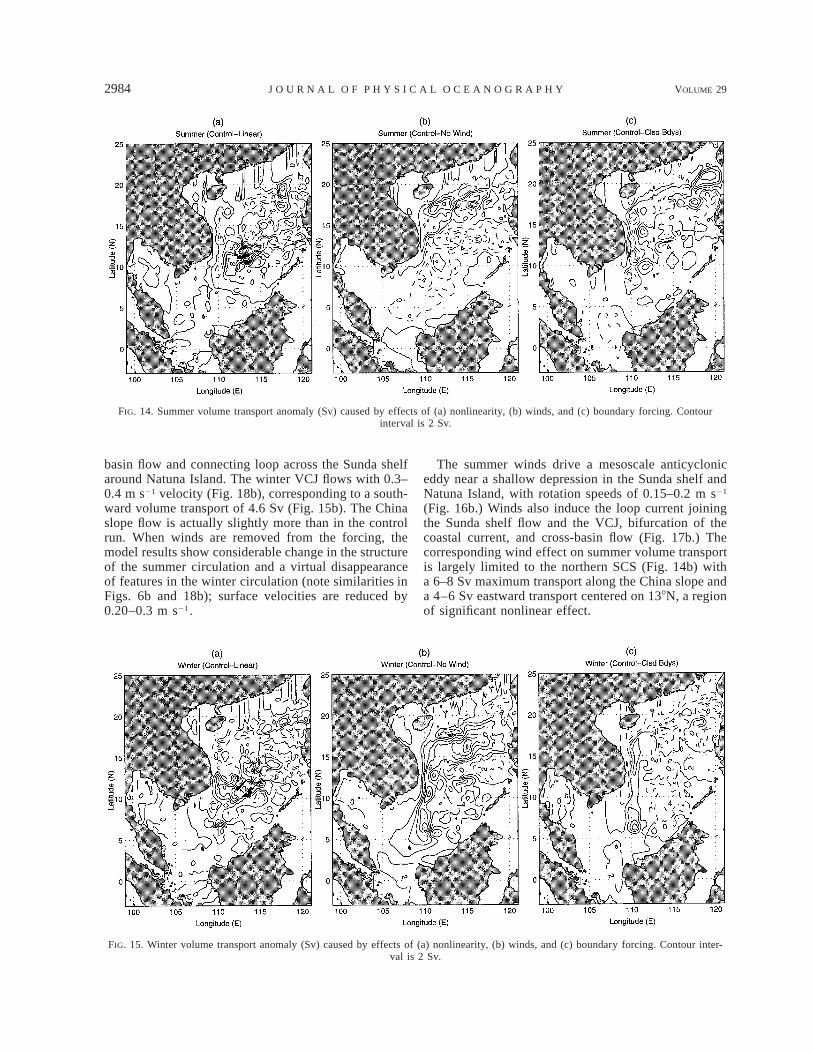
FIG. 14. Summer volume transport anomaly (Sv) caused by effects of (a) nonlinearity, (b) winds, and (c) boundary forcing. Contourinterval is 2 Sv.

FIG. 15. Winter volume transport anomaly (Sv) caused by effects of (a) nonlinearity, (b) winds, and (c) boundary forcing. Contour inter-val is 2 Sv.

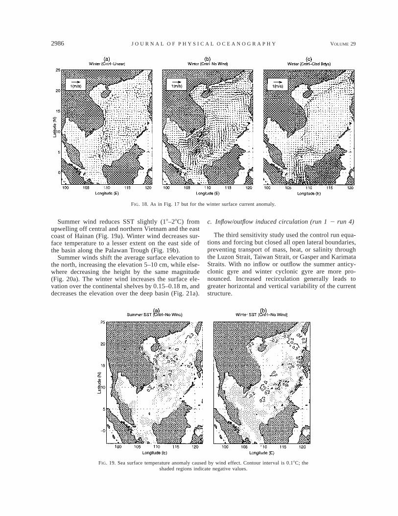
basin flow and connecting loop across the Sunda shelfaround Natuna Island. The winter VCJ flows with 0.3–0.4 m s21 velocity (Fig. 18b), corresponding to a south-ward volume transport of 4.6 Sv (Fig. 15b). The Chinaslope flow is actually slightly more than in the controlrun. When winds are removed from the forcing, themodel results show considerable change in the structureof the summer circulation and a virtual disappearanceof features in the winter circulation (note similarities inFigs. 6b and 18b); surface velocities are reduced by0.20–0.3 m s21.

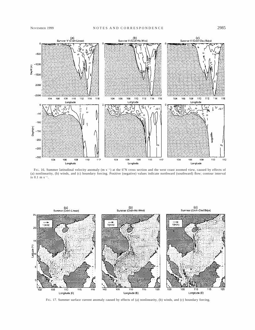
The summer winds drive a mesoscale anticycloniceddy near a shallow depression in the Sunda shelf andNatuna Island, with rotation speeds of 0.15–0.2 m s21

(Fig. 16b.) Winds also induce the loop current joiningthe Sunda shelf flow and the VCJ, bifurcation of thecoastal current, and cross-basin flow (Fig. 17b.) Thecorresponding wind effect on summer volume transportis largely limited to the northern SCS (Fig. 14b) witha 6–8 Sv maximum transport along the China slope anda 4–6 Sv eastward transport centered on 138N, a regionof significant nonlinear effect.


FIG. 16. Summer latitudinal velocity anomaly (m s21) at the 68N cross section and the west coast zoomed view, caused by effects of(a) nonlinearity, (b) winds, and (c) boundary forcing. Positive (negative) values indicate northward (southward) flow; contour intervalis 0.1 m s21 .

FIG. 17. Summer surface current anomaly caused by effects of (a) nonlinearity, (b) winds, and (c) boundary forcing.


FIG. 18. As in Fig. 17 but for the winter surface current anomaly.

FIG. 19. Sea surface temperature anomaly caused by wind effect. Contour interval is 0.18C; theshaded regions indicate negative values.

Summer wind reduces SST slightly (18–28C) fromupwelling off central and northern Vietnam and the eastcoast of Hainan (Fig. 19a). Winter wind decreases sur-face temperature to a lesser extent on the east side ofthe basin along the Palawan Trough (Fig. 19b).

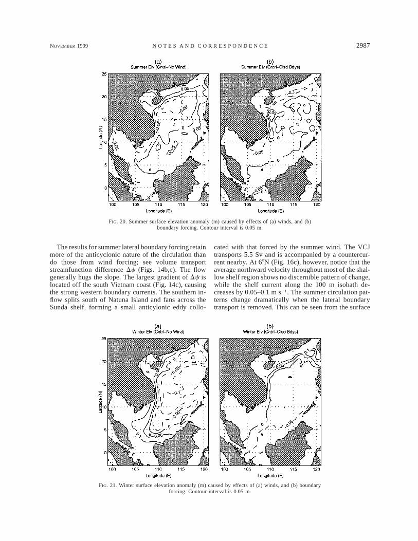
Summer winds shift the average surface elevation tothe north, increasing the elevation 5–10 cm, while else-where decreasing the height by the same magnitude(Fig. 20a). The winter wind increases the surface ele-vation over the continental shelves by 0.15–0.18 m, anddecreases the elevation over the deep basin (Fig. 21a).

c. Inflow/outflow induced circulation (run 1 2 run 4)

The third sensitivity study used the control run equa-tions and forcing but closed all open lateral boundaries,preventing transport of mass, heat, or salinity throughthe Luzon Strait, Taiwan Strait, or Gasper and KarimataStraits. With no inflow or outflow the summer anticy-clonic gyre and winter cyclonic gyre are more pro-nounced. Increased recirculation generally leads togreater horizontal and vertical variability of the currentstructure.


FIG. 20. Summer surface elevation anomaly (m) caused by effects of (a) winds, and (b)boundary forcing. Contour interval is 0.05 m.

FIG. 21. Winter surface elevation anomaly (m) caused by effects of (a) winds, and (b) boundaryforcing. Contour interval is 0.05 m.

The results for summer lateral boundary forcing retainmore of the anticyclonic nature of the circulation thando those from wind forcing; see volume transportstreamfunction difference Dc (Figs. 14b,c). The flowgenerally hugs the slope. The largest gradient of Dc islocated off the south Vietnam coast (Fig. 14c), causingthe strong western boundary currents. The southern in-flow splits south of Natuna Island and fans across theSunda shelf, forming a small anticylonic eddy collo-

cated with that forced by the summer wind. The VCJtransports 5.5 Sv and is accompanied by a countercur-rent nearby. At 68N (Fig. 16c), however, notice that theaverage northward velocity throughout most of the shal-low shelf region shows no discernible pattern of change,while the shelf current along the 100 m isobath de-creases by 0.05–0.1 m s21. The summer circulation pat-terns change dramatically when the lateral boundarytransport is removed. This can be seen from the surface


velocity vector difference DV (Fig. 17c). There is stillwestern intensification of the current along the coast ofMalaysia, and it still joins the flow out of the Gulf ofThailand to contribute to an intensification of currentoff southern Vietnam.

Winter closed boundary circulation patterns, on theother hand, show less difference in structure from thecontrol run but more variability in magnitude. There isan average decrease of 0.1–0.4 m s21 in current speedof the winter VCJ, which equates to 4–6 Sv southwardvolume transport (Fig. 15c). The Kuroshio intrusion andinflow through Taiwan Strait are obviously supple-mented by recirculation flow from along the coast ofLuzon Island. Near Natuna Island it is noteworthy thatthe structure of cross-basin circulation and current flowaway from the Borneo coast are unchanged. Similarly,it is apparent that the spatial extent and shape of thegyre northeast of Natuna Island is unchanged by closingthe boundary flow. In cross section, however, it can beseen that the NIE does lose some of its velocity—thereis a 0.1–0.3 m s21 decrease in the average core velocityon the western side at 68N in this run corresponding toa volume transport of 3 Sv, associated with the decreasein velocity of the VCJ. The difference in velocity ismuch smaller on the eastern side, suggesting that someother effect dominates the current structure in that re-gion.

The summer lateral boundary transport decreases theaverage surface elevation over the China–Vietnam con-tinental shelf by 0.05–0.15 m, while elsewhere increasesthe height with a maximum accretion of 0.2–0.4 m nearthe Karimata Strait (Fig. 20b). The winter lateral bound-ary transport increases the average surface elevationover the China–Vietnam continental shelf by 0.05–0.2m, while elsewhere decreases the height with a maxi-mum reduction of 0.25 m near the Karimata Strait (Fig.21b).

5. Conclusions

1) The SCS circulation and thermohaline structurewas simulated in this study by the POM model underthe climatological forcing. During the summer (winter)monsoon period the SCS surface circulation is generallyanticyclonic (cyclonic) with a strong western boundarycurrent (width around 100 km)—the Vietnam coastaljet. This jet has a strong seasonal variation and flowsnorthward (southward) during summer (winter) with amean maximum speed of 0.5 m s21 (0.95 m s21), witha mean volume transport of 5.5 Sv (10.6 Sv) extendingto a depth of around 200 m (500 m). During summer,the western boundary current splits and partially leavesthe coast; the bifurcation point is at 148N in May andshifts south to 108N in July. The cross-basin zonal cur-rent reaches 128N and a core speed of 0.6 m s21 by theend of the summer. The coastal branch continues north,then east at Hainan Island. Average summer sea surfaceelevation varies from 20.1 to 0.1 m with maximum

values at northeastern part near Luzon. Sea surfaceheights for the winter show a 0.2-m depression over thedeep basin with maximum values in the southwesternpart over the Sunda shelf and the Gulf of Thailand. Thissuggests that the southwest monsoon wind in borealsummer piles up the water at the northeastern part nearLuzon and the northeast monsoon wind in boreal winterpiles up the water at the southwestern part over theSunda shelf and the Gulf of Thailand. The POM modelalso successfully simulates a mesoscale eddy in the Sun-da shelf, namely the Natuna Island eddy. This eddy iscyclonic (anticyclonic) with maximum swirl velocity of0.6 m s21 at the peak of the winter (summer) monsoon.

Isotherms and isohalines for summer and winter arenearly horizontal from east to west except at the coastalregions. Coastal upwelling and downwelling are alsosimulated: localized lifting (descending) of the iso-therms and isohalines during summer (winter) at thewest boundary. Both coastal upwelling and downwell-ing (causing horizontal thermohaline gradient), com-bined with the high velocity shear across the coastal jet,results in baroclinic instability. This mechanism maycontribute to the summer jet bifurcation. In general mod-el thermohaline structure is consistent with the two SCSwater masses described by Wyrtki (1961.) Over thesouthern basin there is a general lifting of isotherms of40–50 m from winter to summer above 200 m. In thenorthern SCS, near-surface waters (20–50 m) are influ-enced by the winter inflow of North Pacific Kuroshiowater.

2) The model wind effects on the SCS are more per-vasive than those of nonlinear dynamic effects. Similarto nonlinear effects there are areas of anticylonic volumetransport midbasin in the summer and winter, althoughthe midbasin surface currents reverse. Summer windeffects on transport are generally divided along the axisof the monsoon wind, SW–NE, with anticyclonicity andpositive elevation in the southeast and cyclonic transportand negative elevation in the northwest. The winter windeffect is largely cyclonic, including a center (with astrong surface current signature) for the NIE, with amatching steeper depression in surface elevation.

3) The model boundary forcing effect on volumetransport is most easily distinguished as anticyclonic inthe summer and cyclonic in the winter. The strongertransport centers of both seasons have strong surfacecurrent signatures including the NIE. Topographicallylinked eddy flow and transport is evident in the summer,while winter flow narrowly follows the 200-m isobathuntil it encounters the Sunda shelf and Natuna Island.

In the summer, SCS volume transport is mostly dueto boundary forcing. Surface movement is marginallydominated by wind forcing, when the boundary-forcingsurface effect (away from the southern boundary) co-alesces with associated volume transport. Winds drivethe offshore summer bifurcation of the VCJ. The anti-cylonic gyre south of Hainan is a surface phenomena


driven by boundary flow interaction with topographyand nonlinear dynamics.

In the winter, surface movement due to boundaryforcing is largely limited to the perimeter of the SCSbasin, specifically a narrow swath over the 200-m iso-bath, away from the southern boundary. Surface flowand volume transport are dominated by the wind effectexcept at the NIE, a mesoscale feature that must bequalified by nonlinear dynamics. Also to be qualifiedby nonlinear dynamics is cross-basin transport for bothseasons.

4) Future studies should concentrate on less simplis-tic scenarios. Realistic lateral transport (especially at theMindoro and Karimata Straits) and surface heat and saltfluxes should be included, and the use of extrapolatedclimatological winds needs to be upgraded to incor-porate synoptic winds to improve realism. Finally, theassumption of quasi linearity that allowed us to usesimple difference to quantify the effect of external forc-ing needs to be rigorously tested. It is very importantto develop a thorough methodology to perform sensi-tivity studies under the highly nonlinear conditions thatmay exist in the littoral environment.

Acknowledgments. The authors wish to thank GeorgeMellor and Tal Ezer of the Princeton University for mostkindly proving us with a copy of the POM code and tothank Laura Ehret for programming assistance. Thiswork was funded by the Office of Naval ResearchNOMP Program, the Naval Oceanographic Office, andthe Naval Postgraduate School.

REFERENCES

Blumberg, A., and G. Mellor, 1987: A description of a three-dimen-sional coastal ocean circulation model. Three-DimensionalCoastal Ocean Models, N. S. Heaps, Ed., Amer. Geophys. Union,1–16.

Chen, J., Z. Fu, and F. Li, 1982: A study of upwelling over Minnan–Taiwan shoal fishing ground. Taiwan Strait, 1, 5–13.

Chu, P. C., and C. P. Chang, 1997: South China Sea warm pool inboreal spring. Adv. Atmos. Sci., 14, 195–206., C. C. Li, D. S. Ko, and C. N. K. Mooers, 1994: Response ofthe South China Sea to seasonal monsoon forcing. Proc. SecondInt. Conf. on Air–Sea Interaction and Meteorology and Ocean-ography of the Coastal Zone, Lisbon, Portugal, Amer. Meteor.Soc., 214–215., M. Huang, and E. Fu, 1996: Formation of the South China Sea

warm core eddy in boreal spring. Proc. Eighth Conf. on Air–Sea Interaction, Atlanta, GA, Amer. Meteor. Soc., 155–159., H.-C. Tseng, C. P. Chang, and J. M. Chen, 1997a: South ChinaSea warm pool detected in spring from the Navy’s Master Ocean-ographic Observational Data Set (MOODS). J. Geophys. Res.,102, 15 761–15 771., S.-H. Lu, and Y.-C. Chen, 1997b: Temporal and spatial vari-abilities of the South China Sea surface temperature anomaly.J. Geophys. Res., 102, 20 937–20 955., C. W. Fan, C. J. Lozano, and J. L. Kirling, 1998: An airborneexpandable bathythermograph survey of the South China Sea,May 1995. J. Geophys. Res., 103, 21 637–21 652.

Courant, R., K. O. Friedrichs, and H. Levy, 1928: Uber die partiellendifferenzengleichungen der mathematischen physik. Math. An-nal., 100, 32–74.

Hellerman, S., and M. Rosenstein, 1983: Normal monthly wind stressover the world ocean with error estimates. J. Phys. Oceanogr.,13, 1093–1104.

Hu, J., and M. Liu, 1992: The current structure during summer insouthern Taiwan Strait (in Chinese). Tropic Oceanology, 11, 42–47.

Huang, Q. Z., W. Z. Wang, Y. S. Li, and C. W. Li, 1994: Currentcharacteristics of the South China Sea. Oceanology of ChinaSeas, Z. Di, L. Yuan-Bo, and Z. Cheng-Kui, Eds., Kluwer, 39–46.

Levitus, S., 1984: Climatological Atlas of the World Ocean, NOAAProf. Paper No. 13, U.S. Gov. Printing Office, 173 pp.

Li, R.-F., D.-J. Guo, and Q.-C. Zeng, 1996: Numerical simulation ofinterrelation between the Kuroshio and the current of the north-ern South China Sea. Prog. Natural Sci., 6, 325–332.

Ma, B.-B., 1998: The South China Sea thermohaline structure andcirculation. Masters thesis, Naval Postgraduate School, Monte-rey, California, 254 pp.

Mellor, G., and T. Yamada, 1982: Development of a turbulence clo-sure model for geophysical fluid problems. Rev. Geophys. SpacePhys., 20, 851–875., and T. Ezer, 1991: A Gulf Stream model and an altimetryassimilation scheme. J. Geophys. Res., 96, 8779–8795.

Metzger, E. J., and H. Hurlburt, 1996: Coupled dynamics of the SouthChina Sea, the Sulu Sea, and the Pacific Ocean. J. Geophys.Res., 101, 12 331–12 352.

Oey, L., and P. Chen, 1991: Frontal waves upstream of a diabaticblocking: A model study. J. Geophys. Res., 21, 1643–1663.

Pohlmann, T., 1987: A three-dimensional circulation model of theSouth China Sea. Three-Dimensional Models of Marine and Es-tuarine Dynamics, J. Nihoul and B. Jamart, Eds., Elsevier Sci-ence, 245–268.

Smagorinsky, J., 1963: General circulation experiments with theprimitive equations, I. The basic experiment. Mon. Wea. Rev.,91, 99–164.

Wyrtki, K., 1961: Scientific results of marine investigations of theSouth China Sea and the Gulf of Thailand 1959–1961. NagaReport, Vol. 2, University of California at San Diego, 164–169.

Yanagi, T., T. Takao, and A. Morimoto, 1997: Co-tidal and co-rangecharts in the South China Sea derived from satellite altimetrydata. La mer, 35, 85–93.

NOTES AND CORRESPONDENCE Dynamical Mechanisms …faculty.nps.edu/pcchu/web_paper/jpo/edmons.pdf ·...

Documents

Transcript of NOTES AND CORRESPONDENCE Dynamical Mechanisms …faculty.nps.edu/pcchu/web_paper/jpo/edmons.pdf ·...