Noisy continuous time random walksJae-Hyung Jeon, Eli Barkai, and Ralf Metzler Citation: J. Chem. Phys. 139, 121916 (2013); doi: 10.1063/1.4816635 View online: http://dx.doi.org/10.1063/1.4816635 View Table of Contents: http://jcp.aip.org/resource/1/JCPSA6/v139/i12 Published by the AIP Publishing LLC. Additional information on J. Chem. Phys.Journal Homepage: http://jcp.aip.org/ Journal Information: http://jcp.aip.org/about/about_the_journal Top downloads: http://jcp.aip.org/features/most_downloaded Information for Authors: http://jcp.aip.org/authors

Downloaded 31 Aug 2013 to 129.128.216.34. This article is copyrighted as indicated in the abstract. Reuse of AIP content is subject to the terms at: http://jcp.aip.org/about/rights_and_permissions

THE JOURNAL OF CHEMICAL PHYSICS 139, 121916 (2013)

Noisy continuous time random walksJae-Hyung Jeon,1,a) Eli Barkai,2,b) and Ralf Metzler1,3,c)

1Department of Physics, Tampere University of Technology, FI-33101 Tampere, Finland2Department of Physics, Bar Ilan University, Ramat-Gan 52900, Israel3Institute for Physics and Astronomy, University of Potsdam, D-14476 Potsdam-Golm, Germany

(Received 7 May 2013; accepted 11 July 2013; published online 31 July 2013)

Experimental studies of the diffusion of biomolecules within biological cells are routinely confrontedwith multiple sources of stochasticity, whose identification renders the detailed data analysis of singlemolecule trajectories quite intricate. Here, we consider subdiffusive continuous time random walksthat represent a seminal model for the anomalous diffusion of tracer particles in complex environ-ments. This motion is characterized by multiple trapping events with infinite mean sojourn time.In real physical situations, however, instead of the full immobilization predicted by the continuoustime random walk model, the motion of the tracer particle shows additional jiggling, for instance,due to thermal agitation of the environment. We here present and analyze in detail an extension ofthe continuous time random walk model. Superimposing the multiple trapping behavior with addi-tive Gaussian noise of variable strength, we demonstrate that the resulting process exhibits a richvariety of apparent dynamic regimes. In particular, such noisy continuous time random walks mayappear ergodic, while the bare continuous time random walk exhibits weak ergodicity breaking. De-tailed knowledge of this behavior will be useful for the truthful physical analysis of experimentallyobserved subdiffusion. © 2013 AIP Publishing LLC. [http://dx.doi.org/10.1063/1.4816635]

I. INTRODUCTION

In a series of experiments in the Weitz lab at Harvard,Wong et al.1 observed that the motion of plastic tracer mi-crobeads in a reconstituted mesh of cross-linked actin fila-ments is characterized by anomalous diffusion of the form

〈r2(t)〉 =∫

r2P (r, t)dr � Kαtα (1)

of the ensemble averaged mean squared displacement (MSD).Here, Kα is the anomalous diffusion constant of physical di-mension [Kα] = cm2/sα , and the anomalous diffusion expo-nent α is in the subdiffusive range 0 < α < 1. P (r, t) is theprobability density function to find the test particle at posi-tion r at time t. Wong et al. demonstrated that the motion ofthe microbeads is represented by a random walk with subse-quent immobilization events of the beads in “cages” withinthe network.1 The durations τ of these immobilization peri-ods were shown to follow the distribution

ψ(τ ) ∼ τα0

τ 1+α, (2)

with the scaling exponent α. The exponent α turns out to bea function of the ratio between the bead size and the typicalmesh size. Thus, when the bead size is larger than the meshsize, the bead becomes fully immobilized, α = 0. Conversely,when the bead is much smaller than the typical mesh size, itmoves like a Brownian particle [α = 1, in Eq. (1)], almostundisturbed by the actin mesh. However, when the bead size

a)Electronic mail: jae-hyung.jeon@tut.fib)Electronic mail: barkaie@mail.biu.ac.ilc)Ralf Metzler contributed to the special issue on Chemical Physics

of Biological Systems. Electronic mail: rmetzler@uni-potsdam.de

is comparable to the mesh size, the motion of the bead is im-peded by the mesh, giving rise to a saltatory bead motion inbetween cages. While the measured distribution (2) of immo-bilization times indeed captures the statistics of the long timemovement of the beads, the measured trajectories also exhibitan additional noise, superimposed to the jump motion accord-ing to the law (2).1 This additional noise is visible as jigglingaround a typical position during sojourn periods of the bead,and appears like regular white noise.

Above example is representative for the task of physi-cal analysis of single particle tracking experiments. Indeed,following single particles such as large labeled molecules,viruses, or artificial tracers in the environment of living cellshas become a standard technique in many laboratories, sinceit reveals the individual trajectories without the problem ofensemble averaging. However, the large amount of poten-tially noisy data also poses a practical challenge. In physicsand mathematics, ideal stochastic processes have been in-vestigated for many years, including Brownian motion, frac-tional Brownian motion (FBM), continuous time randomwalks (CTRW), Lévy flights, etc. While these can be rea-sonable approximations for the physical reality, they rarelyrepresent the whole story. In many cases, a superposition ofat least two types of stochastic motion is found, such as the“contamination” of the pure stop-and-go motion described bythe waiting time distribution (2) with additional noise in theabove example of the tracer beads in the actin mesh. Sim-ilarly, Weigel et al. in their study of protein channel mo-tion in the walls of living human kidney cells observed asuperposition of stochastic motion governed by the law (2),and motion patterns corresponding to diffusion on a fractal.2

Tabei et al. show that the motion of insulin granules in liv-ing MIN6 cells is best explained by a hybrid model in which

0021-9606/2013/139(12)/121916/15/$30.00 © 2013 AIP Publishing LLC139, 121916-1

Downloaded 31 Aug 2013 to 129.128.216.34. This article is copyrighted as indicated in the abstract. Reuse of AIP content is subject to the terms at: http://jcp.aip.org/about/rights_and_permissions

121916-2 Jeon, Barkai, and Metzler J. Chem. Phys. 139, 121916 (2013)

fractional Brownian motion is subordinated to continuoustime random walk subdiffusion.3 Finally, Jeon et al. find thatthe motion of lipid granules in living yeast cells is governedby continuous time random walk motion at short times, turn-ing over to fractional Brownian motion at longer times.4 Evenif the trajectories are ideal, in the lab we always have todeal with additional sources of noise, for instance, the mo-tion within the sample may become disturbed by a slow, ran-dom drift of the object stage in the microscope setup, orsimply by the diffusive motion on the cover slip of a livingcell, inside which the actual motion occurs that we want tofollow.

In recent years, a tool box for data analysis was devel-oped by several groups, in particular, in the context of diffu-sion of tracers in the microscopic cellular environment. Thesealso include fundamental aspects of statistical physics suchas the ergodic properties of the underlying process and theirreproducible nature of the time averages of the data.5 How-ever, to the best of our knowledge these analysis methods andthe fundamental properties of statistical mechanics (that is,ergodicity) have not been tested in the presence of additionalnoise. For instance, if we encounter a non-ergodic process su-perimposed with an ergodic one, as defined precisely below,what will we find as the result of such an experiment? Here,we develop and study in detail a new framework for the mo-tion of a test particle, the noisy continuous time random walk(nCTRW) subject simultaneously to a power-law distribution(2) of sojourn times and additional Gaussian noise. Interest-ingly, the noise turns out to have a dramatic effect on the timeaveraged MSD, typically evaluated in single particle track-ing experiments, but a trivial effect on the ensemble averagedMSD. We hope that this contribution will be a step towardsmore realistic modeling of trajectories of single molecules,but also of other diffusive motions of particles in complexenvironments.

Our analysis is based on two different scenarios for theadditional Gaussian noise. Thus, we will consider (i) a reg-ular diffusive motion (Wiener process) on top of the power-law sojourn times (2). This scenario mirrors effects suchas the diffusion on the cover slip of the biological cell, inwhich the actual motion occurs that we want to monitor. (ii)We study an Ornstein-Uhlenbeck noise with a typical ampli-tude, which may reflect an intrinsically noisy environment,such as in the case of the tracer beads in the actin network.We will study the MSD of the resulting motion both in thesense of the conventional ensemble average and, for its rel-evance in the analysis of single particle tracking measure-ment, the time average. Moreover, we demonstrate how avarying strength of the additional noise may blur the resultof stochastic diagnosis methods introduced recently, such asthe scatter of amplitudes of time averaged MSDs around theaverage over an ensemble of trajectories, or the p-variationmethod.

The paper is organized as follows. In Sec. II A, webriefly discuss the concepts of anomalous diffusion and sin-gle particle tracking along with the role of (non-)ergodicityin the context of ensemble versus time averaged MSDs. InSec. II B, we review some methods of single particle track-ing analysis. Section III then introduces our nCTRW model

consisting of a random walk with long sojourn times super-imposed with Gaussian noise, and we explain the simulationscheme. The main results and discussions are presented inSecs. IV and V: in Sec. IV, we study the statistical behav-ior of nCTRW motion in the presence of superimposed freeBrownian motion, while Sec. V is devoted to the motion dis-turbed by Ornstein-Uhlenbeck noise. Finally, the conclusionsand an outlook are presented in Sec. VI. In the Appendix, weprovide a brief outline of the stochastic analysis tools usedto quantify the nCTRW processes studied in Secs. IV and V.Note that in the following, for simplicity, we concentrate onthe one-dimensional case; all results can easily be generalizedto higher dimensions.

II. ANOMALOUS DIFFUSION AND SINGLEPARTICLE TRACKING

In this section, we briefly review the CTRW model andthe behavior of CTRW time series. Moreover, we presentsome common methods to analyze traces obtained from singleparticle tracking experiments or simulations.

A. Continuous time random walks and time-averagedmean squared displacement

Anomalous diffusion of the subdiffusive form (1) with0 < α < 1 is quite commonly observed in a large varietyof systems and on many different scales.6–12 A prominentmodel to describe the subdiffusion law (1) is given by theMontroll-Weiss-Scher CTRW.13, 14 Originally applied to de-scribe extensive data from the stochastic motion of chargecarriers in amorphous semiconductors,13 the CTRW modelfinds applications in many areas. Inter alia, CTRW subdif-fusion was shown to underlie the motion of microbeads inreconstituted actin networks,1 the subdiffusion of lipid gran-ules in living yeast cells4, 15 of protein channels in human kid-ney cells,2 and of insulin granules in MIN6 cells,3 as wellas the temporal spreading of tracer chemicals in groundwateraquifers.16, 17 While the sojourn times in a subdiffusive CTRWfollow the law (2), the length of individual jumps is governedby a distribution λ(x) of jump lengths, with finite varianceσ 2 = ∫

x2λ(x)dx. In the simplest case of a jump process on alattice, each jump is of the length of the lattice constant. Phys-ically, the power-law form (2) of sojourn times may arise dueto multiple trapping events in a quenched energy landscapewith exponentially distributed depths of traps.18, 19 Subdiffu-sive CTRWs macroscopically exhibit long-tailed memory ef-fects as characterized by the dynamic equation for the proba-bility density function P(x, t) containing fractional differentialoperators, see below.20

Usually, we think in terms of the ensemble average (1)when we talk about the MSD of a diffusive process. How-ever, starting with Nordlund’s seminal study of the Brow-nian motion of a slowly sedimenting mercury droplet21

and now routinely performed even on the level of singlemolecules,1–4, 10, 15, 22–29 the time series x(t) obtained frommeasuring the trajectory of an individual particle is evaluated

Downloaded 31 Aug 2013 to 129.128.216.34. This article is copyrighted as indicated in the abstract. Reuse of AIP content is subject to the terms at: http://jcp.aip.org/about/rights_and_permissions

121916-3 Jeon, Barkai, and Metzler J. Chem. Phys. 139, 121916 (2013)

in terms of the time averaged MSD,

δ2(�) = 1

T − �

∫ T −�

0(x(t + �) − x(t))2dt, (3)

where � is the so-called lag time, and T is the overallmeasurement time. For Brownian motion, the time averagedMSD (3) is equivalent to the ensemble averaged MSD (1),〈x2(�)〉 = δ2(�), if only the measurement time T is suffi-ciently long to ensure self-averaging of the process along thetrajectory. This fact is a direct consequence of the ergodic na-ture of Brownian motion.5, 30 To obtain reliable behaviors forthe time averaged MSD for trajectories with finite T, one oftenintroduces the average

⟨δ2(�)

⟩= 1

N

N∑i=1

δ2i (�) (4)

over several individual trajectories δ2i (�).

What happens when the process is anomalous, of theform (1)? There exist anomalous diffusion processes that areergodic in the above sense that for sufficiently long T weobserve the equivalence 〈x2(�)〉 = δ2(�). Prominent exam-ples are given by diffusion on random fractal geometries,31 aswell as fractional Brownian motion and the related fractionalLangevin equation motion for which ergodicity is approachedalgebraically.32–35 Such behavior was in fact corroborated inparticle tracking experiments in crowded environments23–25

and simulations of lipid bilayer systems.36, 37 In superdiffu-sive Lévy walks time and ensemble averaged MSDs differmerely by a factor.38–40 However, the diverging sojourn timein the subdiffusive CTRW processes naturally causes weakergodicity breaking in the sense that even for extremely longmeasurement time T, ensemble and time averages no longercoincide.41–43 For the time averaged MSD, the consequencesare far-reaching. Thus, for subdiffusive CTRWs, we find thesomewhat counterintuitive result that the time averaged MSDfor free motion (unbiased motion in unbounded space) scaleslinearly with the lag time, 〈δ2(�,T )〉 � Kα�/T 1−α for �

� T, and thus 〈x2(�)〉 �= δ2(�).44, 45 In particular, the result〈δ2(�)〉 decreases with the measurement time T, an effect ofageing. Concurrently, the MSD of subdiffusive CTRWs de-pends on the time difference between the preparation of thesystem and the start of the measurement.46 Under confine-ment, while the ensemble averaged MSD saturates towardsthe thermal value, the time averaged MSD continues to growas 〈δ2(�)〉 � �1−α as long as � � T.47, 48 Another impor-tant consequence of the weakly non-ergodic behavior is thatthe time averaged MSD (3) remains irreproducible even inthe limit of T → ∞: the amplitude of individual time aver-aged MSD curves δ2

i (�) scatters significantly between differ-ent trajectories, albeit with a well-defined distribution.44, 49, 50

In other words, this scatter of amplitudes corresponds to anapparent distribution of diffusion constants.51 Active trans-port of molecules in the cell exhibits superdiffusion with non-reproducible results for the time averages,52 a case treated the-oretically only recently.39, 40, 53

To pin down a given stochastic mechanism underlyingsome measured trajectories, several diagnosis methods havebeen developed. Thus, one may analyze the first passagebehavior,54 moment ratios and the statistics of mean maximalexcursions,55 the velocity autocorrelation,30, 37 the statistics ofthe apparent diffusivities,56 or the p-variation of the data.57, 58

In the following, we analyze the sensitivity of the time aver-aged MSD and its amplitude scatter as well as the p-variationmethod to noise, that is superimposed to bare subdiffusiveCTRWs. In particular, we show that at larger amplitudes ofthe additional noise, the CTRW-inherent weak non-ergodicitymay become completely masked.

B. A primer on single particle trajectory analysis

Before proceeding to define the nCTRW process, wepresent a brief review of several techniques developed re-cently for the analysis of single particle trajectories.

1. Mean-squared displacement

Already from the time averaged MSD δ2i of individual

particle traces, important information on the nature of the pro-cess may be extracted, provided that the measurement time Tis sufficiently long. Thus, for ergodic processes, the time andensemble averaged MSDs are equivalent, δ2(�) = 〈x2(�)〉. Asignificant difference between both quantities points at non-ergodic behavior. In particular, the scatter of amplitudes (dis-tribution of diffusion constants) between individual tracesδ2i turns out to be a quite reliable measure for the (non-)

ergodicity of a process. Thus, in terms of the dimensionlessparameter ξ = δ2/〈δ2〉, the distribution of amplitudes φ(ξ )has a Gaussian profile centered on the ergodic value ξ = 1for finite-time ergodic processes.59 Its width narrows with in-creasing T, eventually approaching the sharp distribution δ(ξ− 1) at T → ∞, i.e., each trajectory gives exactly the sameresult, equivalent to the ensemble averaged MSD. For subdif-fusive CTRW processes, φ(ξ ) is quite broad and has a finitevalue at ξ = 0 for completely stalled trajectories.30, 44, 46, 49, 59

For α ≤ 1/2, the maximum of the distribution is at ξ = 0,while for α > 1/2 the maximum is located at ξ = 1. The non-Gaussian distribution φ(ξ ) for subdiffusive CTRWs is almostindependent of T, and its shape is already well establishedeven for relatively short trajectories.59

2. p-variation test

The p-variation test was recently promoted as a tool todistinguish CTRW and FBM-type subdiffusion.57 It is definedin terms of the sum of increments of the trajectory x(t) on theinterval [0, T] as

V (p)n (t) =

2n−1∑j=0

∣∣∣∣x(

(j + 1)T

2n∧ t

)− x

(jT

2n∧ t

)∣∣∣∣p

, (5)

where a∧b = min{a, b}. The quantity V (p) = limn→∞ V(p)n

has distinct properties for certain stochastic processes. Thus,for both free and confined Brownian motion, V (2)(t) ∼ t and

Downloaded 31 Aug 2013 to 129.128.216.34. This article is copyrighted as indicated in the abstract. Reuse of AIP content is subject to the terms at: http://jcp.aip.org/about/rights_and_permissions

121916-4 Jeon, Barkai, and Metzler J. Chem. Phys. 139, 121916 (2013)

FIG. 1. Results of the p-variation test for (a) Brownian noise zB(t), (b) Ornstein-Uhlenbeck noise zOU(t), and (c) subdiffusive CTRW xα(t) with α = 0.5. Theleft panels in each case are for p = 4 for both (a) and (b), and (c) p = 2/α = 4. All right panels are for p = 2. The color coding refers to the values of n indicatedin the right panel of each pair of graphs.

V (p)(t) = 0, for any p > 2. For fractional Brownian motion,V (2)(t) = ∞, while V (2/α)(t) ∼ t . Finally, for CTRW subd-iffusion, V (2)(t) features a step-like, monotonic increase asfunction of time t, and V (2/α)(t) = 0.

Figure 1 shows the p-variation results for Brownian noisezB(t), Ornstein-Uhlenbeck noise zOU(t), and the bare subdif-fusive CTRW xα(t). We plot the sum (5) for various, finitevalues of n. For the Brownian noise zB(t), V (4)

n monotonicallydecreases with growing n, a signature of the predicted con-vergence to V (4) → 0. The sum V (2) appears independent ofn and proportional to time t, as expected. For the Ornstein-Uhlenbeck noise zOU(t), we observe that V (4) scales linearlywith t and the slope decreases with growing n, indicating aconvergence to zero. Also V (2) is linear in t. For smaller n,the slope increases with n and saturates at large n. Finally,for CTRW subdiffusion, V (2/α) appears to converge to zerofor increasing n, as predicted. By contrast, V (2) has the dis-tinct, monotonic step-like increase expected for CTRW sub-diffusion. A more detailed description of the p-variation forOrnstein-Uhlenbeck noise and CTRW subdiffusion is foundin the Appendix.

III. NOISY CONTINUOUS TIME RANDOM WALK

In this section, we define the nCTRW model and describeour simulations scheme.

A. Two nCTRW models—Drifting versus rattling

We consider an nCTRW process x(t) in which ordinaryCTRW subdiffusion xα(t) with anomalous diffusion exponent0 < α < 1 is superimposed with the Gaussian noise ηz(t),

x(t) = xα(t) + ηz(t). (6)

That means that the Gaussian process z(t) is additive and thusindependent of xα(t). The relative strength of the additionalGaussian noise is controlled by the amplitude parameterη ≥ 0. In this study, we consider the following twoGaussian processes: (1) In the first case, z(t) is a simple Brow-nian diffusive process zB(t) with zero mean 〈zB(t)〉 = 0 andvariance 〈z2

B(t)〉 = 2Dt . As mentioned, physically this couldrepresent the (slow) diffusion of a living bacteria or endothe-lial cell on the cover slip while we want to record the motionof a tracer inside the cell, or the random drifting of the exper-imental stage. (2) In the second case, z(t) represents Ornstein-Uhlenbeck noise zOU(t). This Gaussian process corresponds tothe confined Brownian motion in an harmonic potential (seeEq. (18) for the definition of the process). We use this con-fined additive noise to phenomenologically mimic the thermalrattling of the matrix, in which the particle is successivelyimmobilized during waiting periods in the CTRW sense. Inthe example of the tracer bead in the cross-linked actin meshdiscussed in the Introduction, this Ornstein-Uhlenbeck noisecorresponds to the rattling with a constant amplitude aroundsome average position.

Downloaded 31 Aug 2013 to 129.128.216.34. This article is copyrighted as indicated in the abstract. Reuse of AIP content is subject to the terms at: http://jcp.aip.org/about/rights_and_permissions

121916-5 Jeon, Barkai, and Metzler J. Chem. Phys. 139, 121916 (2013)

According to definition (6), nCTRW processes have thefollowing generic properties. Its probability density function(PDF) P(x, t) is given by the convolution of the individualPDFs Pα(x, t) of a CTRW subdiffusion process and PG(x, t)of the Gaussian process,

P (x, t) =∫ ∞

−∞Pα(x − y, t)PG(y, t)dy. (7)

This chain rule states that a given position x of the combinedprocess is given by the product of the probability that theCTRW process has reached the position x-y and the Gaus-sian process contributes the distance y, or vice versa. Here, thePDF Pα(x, t) satisfies the fractional Fokker-Planck equation,8

∂

∂tPα(x, t) = 0D1−α

t Kα

∂2

∂x2Pα(x, t), (8)

where the Riemann-Liouville fractional derivative of Pα(x, t)is

0D1−αt Pα(x, t) = 1

(α)

∂

∂t

∫ t

0

Pα(x, t ′)(t − t ′)1−α

dt ′. (9)

Physically, this fractional operator thus represents a memoryintegral with a slowly decaying kernel. From definition (6), itfollows that the ensemble averaged MSD is given by

〈x2(t)〉 =∫ ∞

−∞x2Pα(x, t)dx +

∫ ∞

−∞y2PG(y, t)dy

= 〈x2α(t)〉 + η2〈z2(t)〉. (10)

The characteristic function of P(x, t) according to Eq. (7) isgiven by the product

P (q, t) =∫ ∞

−∞eiqxP (x, t)dx = Pα(q, t)PG(q, t) (11)

of the characteristic functions of the individual processes, Pα

and PG. We here use the simplified notation that the Fouriertransform of a function is expressed by its explicit dependenceon the Fourier variable q. With the Mittag-Leffler functionEα(x) = ∑∞

m=0 xm/ (1 + αm), we find that8

Pα(q, t) = Eα(−q2Kαtα), (12)

assuming that the CTRW process starts at t = 0 with ini-tial conditions xα(0) = 0. The characteristic function Pα(q,t) initially decays like a stretched exponential Pα(q, t)≈ exp (−q2Kαtα/ (1 + α)), and has the asymptotic power-law decay Pα(q, t) ∼ 1/(q2Kαtα).

The Brownian noise ηzB(t) with initial conditionzB(0) = 0 has the characteristic function

PG(q, t) = exp(−η2Dq2t). (13)

In the nCTRW process, this Brownian noise always dom-inates the dynamics of the process at long times, sincethe exponential relaxation (13) dominates the characteris-tic function P(q, t). The Ornstein-Uhlenbeck noise ηzOU(t)

with zOU(0) = 0, defined in Eq. (18), has the characteristicfunction

PG(q, t) = exp

(−η2Dq2

2k(1 − e−2kt )

). (14)

At short times, t � k−1 when confinement by the harmonicOrnstein-Uhlenbeck potential is negligible, Eq. (14) reducesto the result (13) for Brownian noise, and thus the charac-teristic functions of the two nCTRW processes are identi-cal. At longer times, the characteristic function (14) saturatesto PG(q) = exp [− η2Dq2/(2k)]. This means that the long-time behavior of the nCTRW with superimposed Ornstein-Uhlenbeck noise largely reflects the bare CTRW processxα(t), if the noise level is not too high. Keeping these generalfeatures in mind, we further study the statistical quantities ofthe two nCTRW processes numerically.

B. Simulation of the nCTRW process

To simulate the nCTRW process, we independently ob-tain time traces of the subdiffusive CTRW motion xα(t) andthe additional Gaussian noise. The motion xα(t) with 0 < α

< 1 is generated on a lattice of spacing a from the normalizedwaiting time distribution

ψ(τ ) = α/τ0

(1 + τ/τ0)1+α(15)

with the power-law asymptotic scaling ψ(τ ) ∼ ατα0 /τ 1+α .

Here, τ 0 is a scaling constant of dimension [τ 0] = sec.The jump lengths are determined by the δ-distributionλ(x) = 1

2δ(|x| − a).4, 33 Within this construction, the CTRWprocess is associated with the fractional Fokker-Planck equa-tion (8) with the anomalous diffusion exponent:60

Kα = (1 − α)a2

2τα0

. (16)

In the simulations we choose τ 0 = 1, and consequently inthe following times are given in units of τ 0, which is alsochosen equal to the time increments δt, at which the system isupdated. The lattice spacing is a = 0.1. We simulate the casesα = 0.5 and 0.8.

The added Gaussian noise is produced as follows. Brow-nian noise z(t) = zB(t) is obtained at discrete times tn = nδt(with δt = 1), in terms of the Brownian walk

zB(tn) =n∑

k=1

δt√

2DξB(tk), (17)

where ξB(t) represents white Gaussian noise of zero mean andunit variance 1/δt with our choice δt = 1. In the simulationswe take D = 0.05, such that 〈z2

B(1)〉 = 0.1. The Ornstein-Uhlenbeck noise z(t) = zOU(t) is formally obtained by inte-gration of the overdamped Langevin equation for a particlemoving in an harmonic potential of stiffness k,

d

dtzOU (t) = −kzOU (t) +

√2DξB(t), (18)

with the initial condition zOU(0) = 0. Here, the coefficient ofthe restoring force is chosen as k = 0.01. For both Brownian

Downloaded 31 Aug 2013 to 129.128.216.34. This article is copyrighted as indicated in the abstract. Reuse of AIP content is subject to the terms at: http://jcp.aip.org/about/rights_and_permissions

121916-6 Jeon, Barkai, and Metzler J. Chem. Phys. 139, 121916 (2013)

FIG. 2. Sample trajectories of the nCTRW process xα(t) with superimposed Brownian noise ηzB(t) of strength η, for several values of η, and for anomalousdiffusion exponents (a) α = 0.5 and (b) α = 0.8. With increasing noise strength, the otherwise pronounced sojourn states become increasingly blurred by theBrownian motion. For each α, the CTRW part of the trajectory is identical.

and Ornstein-Uhlenbeck noise, the following values for thenoise strength are used: η = 0.001, 0.005, 0.01, and 0.1.

IV. nCTRW WITH BROWNIAN NOISE

In Fig. 2, we show typical examples of simulated trajec-tories of the nCTRW process x(t) with added Brownian noise.The trajectories x(t) for different noise strengths η are con-structed for the same CTRW process xα(t), i.e., only the noisestrength varies in between the panels. This way it is easierto appreciate the influence of the added noise. We generallyobserve that the trajectories preserve the profile of the un-derlying CTRW process xα(t) at small η, and they becomequite distorted from the original CTRW trajectory xα(t) forlarger values of η. In particular, for the largest noise strengththe character of the pure CTRW with its pronounced stallingevents is completely lost, and visually one might judge thesetraces to be pure Brownian motion, at least when the lengthT of the time series is not too large. Moreover, the effectof the noise is stronger for smaller α. This is because longstalling events occur more frequently as α decreases, and thusthe actual displacement of the process is also smaller and theinfluence of the Brownian motion becomes relatively morepronounced.

A. Ensemble-averaged mean squared displacements

From the simulated trajectories we evaluate theensemble-averaged MSD for the nCTRW and study how itsscaling behavior is affected by the Brownian noise zB(t).Figure 3 summarizes the results for the nCTRW process withα = 0.5 and α = 0.8. In both cases, a common feature isthat the ensemble averaged MSD exhibits a continuous tran-sition from subdiffusion with anomalous diffusion exponentα to normal diffusion. This occurs either as the noise strengthη is increased at fixed time t, or as time t is increased at a fixedη. Due to the additivity of the two contributions, we obtain

〈x2(t)〉 = 2Kα

(1 + α)tα + 2η2Dt, (19)

which is valid as long as t is considerably larger than the timeincrement δt. Equation (19) demonstrates that for the subd-iffusive CTRW processes, xα(t) with 0 < α < 1, the ensem-ble averaged MSD of the nCTRW x(t) has a crossover in itsscaling from �tα at short times to �t at long times, with thecrossover time scale tc ∼ (Kα/[ (1 + α)η2D])1/(1 − α). Thatis, the effect of the Brownian noise zB(t) emerges only atlong times t > tc. Conversely, below tc the process appearsto behave as the bare CTRW process. Note that the crossovertime tc rapidly decreases with increasing η as tc ∼ η−2/(1 − α).This explains why we only observe normal diffusion behaviorwithout crossover for the largest noise strength η = 0.1. Thecrossover time tc also rapidly increases as the exponent α ap-proaches to one [as Kα ∼ (1 − α) in our choice of τ 0 = 1,see Eq. (16)]. Accordingly, in Fig. 3, the ensemble averagedMSDs for α = 0.8 do not fully reach the linear regime within

FIG. 3. (Top) Ensemble averaged MSD of the nCTRW process x(t) withnoise strengths η = 0.001, 0.01, and 0.1 for anomalous diffusion exponents α

= 0.5 (left) and α = 0.8 (right). A crossover from subdiffusive to Brownian(linear) scaling is observed. N = 104 trajectories were used for the averag-ing. (Bottom) Trajectory-averaged time averaged MSD 〈δ2(�)〉 for x(t) forthe same values of η and α. The overall measurement time is T = 105 in unitsof δt and the number of trajectories N = 103.

Downloaded 31 Aug 2013 to 129.128.216.34. This article is copyrighted as indicated in the abstract. Reuse of AIP content is subject to the terms at: http://jcp.aip.org/about/rights_and_permissions

121916-7 Jeon, Barkai, and Metzler J. Chem. Phys. 139, 121916 (2013)

FIG. 4. Ten individual time averaged MSD curves for nCTRW with (a) α = 0.5 and (b) α = 0.8 with added Brownian noise, for the same parameters as inFig. 3. The relative amplitude scatter dramatically reduces at high noise strength, compare Fig. 5.

the time window of our simulation, in contrast to the case forα = 0.5 with η = 0.1.

B. Time-averaged mean squared displacement

We now consider the individual time averaged MSDsδ2(�) of the nCTRW process from single trajectories x(t) ac-cording to our definition in Eq. (3). Figure 3 presents thetrajectory-to-trajectory average (4). In all cases we find thatthe time averaged MSDs grow linearly with lag time � in theentire range of �, showing a clear disparity from the scal-ing behavior of the ensemble averaged MSDs above. In thetime averaged MSD, the Brownian noise zB(t) simply affectsthe apparent diffusion constant, that is, the effective amplitudeof the linear curves. To understand this phenomenon quantita-tively, we obtain the analytical form of the trajectory-averagedtime averaged MSD,

⟨δ2(�)

⟩∼ 2Kα�

(1 + α)T 1−α+ 2η2D�, (20)

valid for � � T. Equation (20) shows that both contributions,the bare CTRW xα(t) and the Brownian process ηzB(t), are lin-early proportional to the lag time �. Note that the exponent α

and the noise strength η only enter into the apparent diffusionconstant

Dapp ≡ KαT α−1

(1 + α)+ η2D, (21)

where 〈δ2(�)〉 = 2Dapp�. This result indicates that the effectof the Brownian noise cannot be noticed when we exclusivelyconsider the scaling behavior of the time averaged MSD. Alsoin terms of the apparent diffusion constant, one hardly noticesthe presence of the Brownian noise component as long as η is

small. This agrees with our observations for the time averagedMSD curves in Fig. 3 for noise strengths η = 0.001 and 0.01.

We also check the fluctuations between individual timeaveraged MSD curves δ2(�). Each panel in Fig. 4 plots ten in-dividual time averaged MSDs for the nCTRW process. In allcases, the individual time averaged MSDs display linear scal-ing with lag time �, namely, the scaling behavior of 〈δ2(�)〉.The individual amplitudes scatter, that is, the apparent diffu-sion constant Dapp fluctuates. With increasing strength of theBrownian component, the relative scatter between individualtrajectories dramatically diminishes, leading to an apparentlyergodic behavior. Thus, for the largest noise strength η = 0.1,the ten trajectories almost fully collapse onto a single curvefor � � T.

C. Scatter distribution

We quantify the amplitude scatter of the individual timeaveraged MSDs in terms of the normalized scatter distribu-tions φ(ξ ), where the dimensionless variable ξ stands for theratio ξ = δ2/〈δ2〉 of individual traces δ2 versus the trajectoryaverage 〈δ2〉 (compare the derivations in Refs. 5, 30, and 44).Figure 5 shows φ(ξ ) for several values of the lag time �.When the noise is negligible (η = 0.001), the observed broaddistribution is nearly that of the pure CTRW process. For α

= 1/2, the distribution has the expected Gaussian profile cen-tered at ξ = 0,44 indicating that long stalling events of the or-der of the entire measurement time T occur with appreciableprobability. In the opposite case η = 0.1, the Brownian noiseresults in a relatively sharply peaked, bell-shaped distributiontypical for ergodic processes, at all lag times. An interestingeffect of the Brownian noise is that at intermediate strengthsit only tends to suppress the contribution at around zero,while it does not significantly change the overall profile of the

Downloaded 31 Aug 2013 to 129.128.216.34. This article is copyrighted as indicated in the abstract. Reuse of AIP content is subject to the terms at: http://jcp.aip.org/about/rights_and_permissions

121916-8 Jeon, Barkai, and Metzler J. Chem. Phys. 139, 121916 (2013)

FIG. 5. Variation of normalized scatter distributions φ(ξ ) as a function ofdimensionless variable ξ = δ2/〈δ2〉 for the cases of η = 0.001 (black square),0.005 (red circle), 0.01 (green upper-triangle), and 0.1 (blue down-triangle).(Upper panels) α = 0.5. (Lower panels) α = 0.8. In each figure the resultswere obtained from 104 runs.

distribution compared to the noise-free case. This implicatesthat the trajectories share non-ergodic and ergodic elements.For instance, the trajectory of the nCTRW process x(t) itselffor η = 0.01 in Fig. 2 shows a substantially blurred profileof the underlying CTRW process xα(t) due to the relativelystrong Brownian noise; however, the time averaged MSD andits distribution do exhibit non-ergodic behavior, as shown inFig. 5. The case α = 0.8 shown in Fig. 5 features similar al-beit less pronounced effects. In particular, φ(ξ ) for the bareCTRW has its maximum at the ergodic value ξ = 1. Again,the effect of the Brownian noise is to suppress the contributionat ξ = 0.

D. p-variation test

We now turn to the p-variation test and investigate itssensitivity to the additional noise in the nCTRW process,in comparison to the established results for the bare CTRWxα(t). From the trajectory x(t), the partial sum V

(p)n (t) is calcu-

lated for finite n according to definition (5), where we choosep = 2/α and p = 2, compare Sec. II B. In Fig. 6, we plotthe results of the p-variation at increasing n for the nCTRWprocess. We observe that for both cases α = 0.5 and 0.8, thep-sums behave analogously to the predictions for the bareCTRW process, as long as the noise strength remains suffi-ciently small, according to Fig. 6 this holds for η = 0.001and 0.005 (not shown). In this case, V

(2/α)n (t) monotonically

decreases with increasing n, indicating the limiting behaviorV

(2/α)n (t) → 0 for large n. Meanwhile, V (2)

n (t) approaches themonotonic step-like behavior typical for the CTRW processxα(t), as n increases. Note that the p-sums have plateaus intheir increments in analogy to the noise-free case due to thelong stalling events in the trajectory.

As the magnitude of the Brownian noise grows larger (η= 0.01 and 0.1), however, the behavior of the p-sums changessignificantly. While V

(2/α)n (t) decreases with increasing n as

for the weaker noise case, it increases linearly with t nearlywithout any sign of plateaus for both nCTRW processes ofα = 0.5 and 0.8 when the noise strength is increased to η

= 0.1. This new feature is the expected behavior of V(p)n (t)

with p > 2 for a Brownian diffusive process (see Sec. II Band Fig. 1). Indeed, it can be shown that for p = 4 the p-sumof the Brownian noise zB(t) behaves as V (4)

n (t) ∼ ( T2n )t . We

note that for the Brownian noise zB(t) the p-sum V(p)n (t) with

p > 2 always decays out to zero as n → ∞. Therefore, thenCTRW process will always have the same p variation resultof V

(2/α)n = 0 (in the limit of n → ∞) as the pure CTRW xα(t),

even in case that its profile is dominated by large noise.By contrast, the p-sum V (2)

n (t) exhibits a more distin-guished effect of the Brownian noise due to the fact that theBrownian noise ηzB(t) has V (2)

n (t) � η22Dt . Especially, wefind that the noise effect is pronounced for the nCTRW withα = 0.5, when the underlying CTRW process xα(t) featuresonly few jumps. In this case, the Brownian noise of moder-ate strength (η = 0.01) causes an incline with almost identicalslope to the step-like profiles of V (2)

n (t). At the strongest noiseη = 0.1, the step-like behavior typical for the bare CTRWprocess xα(t) is nearly masked and the overall tendency fol-lows that of Brownian motion shown in Fig. 1. Accordingly,the p-variation test does not properly pin down the underlyingCTRW process xα(t) and thus potentially produces inconsis-tent conclusion for the nCTRW process. A qualitatively iden-tical behavior is obtained for the nCTRW process when theunderlying CTRW process xα(t) performs relatively frequentjumps (corresponding to the case of α = 0.8). However, herethe effect of the Brownian noise appears weak, because thecontribution of zB(t) relative to the magnitude of xα(t) be-comes smaller at larger α values, see the trajectories x(t) inFig. 2.

V. nCTRW WITH ORNSTEIN-UHLENBECK NOISE

We now turn to nCTRW processes x(t), in which the su-perimposed noise is of Ornstein-Uhlenbeck form (18). In thiscase the influence of the added noise is expected to dimin-ish as the process develops, according to our discussion inSec. III.

Figure 7 shows simulated trajectories for the nCTRWprocess xα(t) with two different anomalous diffusion expo-nents, (a) α = 0.5 and (b) α = 0.8, for different noisestrengths η. Indeed, we observe that compared to case ofBrownian noise depicted in Fig. 2, the profiles of the jumpsand rests of the bare CTRW motion xα(t) are relatively wellpreserved despite the mixing with the Ornstein-Uhlenbecknoise zOU(t). Note that the simulated trajectories with mod-erate noise strength appear quite similar to the experimentaltraces of the microbeads in the reconstituted actin networkreported by Wong et al.1 The noise interference appears con-siderably lesser for the case α = 0.8, when the magnitudeof the net displacements is large relative to the noise contri-bution due to frequent jumps in the trajectory xα(t) when α

is closer to unity. Only for the highest noise strength the pureCTRW behavior with its distinct sojourns becomes blurred bythe Ornstein-Uhlenbeck noise.

Downloaded 31 Aug 2013 to 129.128.216.34. This article is copyrighted as indicated in the abstract. Reuse of AIP content is subject to the terms at: http://jcp.aip.org/about/rights_and_permissions

121916-9 Jeon, Barkai, and Metzler J. Chem. Phys. 139, 121916 (2013)

FIG. 6. Results of the p-variation test for the nCTRW process with Brownian noise ηzB(t) for noise strengths η = 0.001, η = 0.01, and η = 0.1. The upper(lower) two rows are for α = 0.5 and 0.8. In all figures, the p sums are plotted with the same color code: n = 8 (black), 9 (red), 10 (green), 11 (blue), 12 (cyan),13 (violet), and 14 (yellow).

A. Ensemble-averaged mean squared displacement

In Fig. 8, we plot the ensemble averaged MSD 〈x2(t)〉 ofthe nCTRW process with Ornstein-Uhlenbeck noise for dif-ferent noise strengths η. We note that, regardless of the in-tensity η, the ensemble averaged MSDs follow the scalinglaw ∼tα of the noise-free CTRW process xα(t), in particu-

lar, at long times. Moreover, all MSD curves at different η

almost collapse onto each other, although small differencesare discernible at short times. These results suggest that, incontrast to the Brownian noise case discussed in Sec. IV,the Ornstein-Uhlenbeck noise does not critically interferewith the diffusive behavior of the noise-free CTRW motion,as expected. To obtain a quantitative understanding of these

FIG. 7. Sample trajectories of the nCTRW process x(t) with Ornstein-Uhlenbeck noise for several values of the noise strength η and anomalous diffusionexponents (a) α = 0.5 and (b) α = 0.8. In contrast to the Brownian noise case of Fig. 2, however, the approximately constant amplitude of the superimposednoise is characteristic for the Ornstein-Uhlenbeck process.

Downloaded 31 Aug 2013 to 129.128.216.34. This article is copyrighted as indicated in the abstract. Reuse of AIP content is subject to the terms at: http://jcp.aip.org/about/rights_and_permissions

121916-10 Jeon, Barkai, and Metzler J. Chem. Phys. 139, 121916 (2013)

FIG. 8. (Top) Ensemble-averaged MSD 〈x2(t)〉 of the nCTRW process withOrnstein-Uhlenbeck noise for anomalous diffusion exponents α = 0.5 and0.8, from 104 trajectories. (Bottom) Trajectory-average of the time averagedMSD 〈δ2(�)〉 for the same α. We use T = 105 and the number of trajectoriesN = 103.

results, we derive the analytic form of the ensemble averagedMSD,

〈x2(t)〉 = 2Kα

(1 + α)tα + η2D

k(1 − e−2kt ). (22)

Here, the last term stems from the contribution of theOrnstein-Uhlenbeck noise. For t > k−1, it saturates to the con-stant η2D/k, which is typically small relative to 2Kαtα/ (1+ α). Hence, at long times t > k−1, the noise term is neg-ligible, and the ensemble averaged MSD grows as 2Kαtα/ (1+ α), consistent with the observations in Fig. 8. In the oppo-site case for t < k−1, the contribution of the noise is expandedto obtain 〈z2

OU (t)〉 ≈ 2η2Dt . As discussed for the characteris-tic function (14), on these time scales the Ornstein-Uhlenbecknoise zOU(t) has the same form as the Brownian noise zB(t),leading to the same scaling form (19) for the ensemble av-eraged MSD. However, as studied in the previous case, theeffect of the linear scaling is irrelevant at short times.

B. Time-averaged mean squared displacement

We now turn to the time averaged MSD curves δ2(�)from individual trajectories x(t) of the nCTRW process.Figure 8 shows the trajectory-averaged time averaged MSD〈δ2(�)〉 for different noise strengths. For both anomalous dif-fusion exponents α = 0.5 and 0.8, we observe qualitativelythe same behavior. On the one hand, the CTRW motion su-perimposed with moderate noise (η = 0.001 and 0.01) leadsto a linear scaling of the time averaged MSD with lag time�, with almost identical amplitude. On the other hand, whenthe noise amplitude becomes large, the scaling of the timeaveraged MSD is significantly affected. We find that these re-sults are consistent with the analytical form of the trajectory-averaged time averaged MSD,

⟨δ2(�)

⟩∼ 2Kα�

(1 + α)T 1−α+ 2η2D

k(1 − e−k�), (23)

valid at lag times � � T. In this expression, it is worth-while to point out that the contribution of the bare CTRWprocess xα(t) is decreased as the length of the trajectory be-comes longer, due to the aging effect of the decreasing effec-tive diffusion constant �Tα − 1, while the noise is indepen-dent of T. Due to this effect, the time averaged MSD (23)has three distinct scaling regimes: (i) At lag times � � k−1,the time averaged MSD is linearly proportional to the lagtime with apparent diffusion constant Dapp ≈ KαTα − 1/ (1+ α). (ii) At lag times � � k−1, the time averaged MSDis again proportional to �. On this timescale, however, thenoise part cannot be ignored, and the apparent diffusion con-stant is given by Dapp ≈ KαTα − 1/ (1 + α) + η2D. Note thatthe diffusion constant at short lag times is larger than the oneat long times. (iii) For lag times � ≈ k−1, the time averagedMSD is that of confined Brownian diffusion, where 〈δ2(�)〉≈ 2KαT α−1�/ (1 + α) + 2η2D. These three regimes areexpected to occur only in the presence of large noise strengthswhen η2D > KαTα − 1/ (1 + α) (see the case η = 0.1 inFig. 8). In the opposite case, when 2η2D is negligi-ble compared to KαTα − 1/ (1 + α), the three regimesare indistinguishable, and only one scaling law 〈δ2(�)〉≈ 2KαT α−1�/ (1 + α) is observed at all lag times. This be-havior is seen for the two cases of η = 0.001 and 0.01 inFig. 8.

Interestingly, the time averaged MSD for the nCTRWwith anomalous diffusion exponent α = 0.5 and noise strengthη = 0.1 is reminiscent of the MSD curves observed formicron-sized tracer particles immersed in wormlike micel-lar solutions, which are known to behave as a viscoelas-tic polymer network when the micelles concentration isabove a critical value.61 Experiments using diffusing wavespectroscopy62, 63 and single-particle tracking25 revealed thatthe immersed particles exhibit three distinct diffusive behav-iors in different time windows. It was shown that particlessurrounded by the micellar network undergo a Brownian dif-fusion at short (sub-milliseconds) times until they engage withthe caging effects of the micellar network, while at later times(milliseconds to sub-seconds) one observes a seemingly con-fined Brownian motion. It turns out that this confined diffu-sion is in fact a pronounced subdiffusive motion characterizedby anti-persistent spatial correlation induced by the polymer

FIG. 9. Profiles of the time averaged MSD 〈δ2(�, T )〉 as a function of mea-surement time T at a fixed lag time � = 100. We show the nCTRW of α

= 0.5 with ηzOU(t) at η = 0.001, 0.01, and 0.1 (from bottom to top). Solidand dotted lines represent the analytical form (23) and the scaling ∼Tα − 1,respectively. N = 103 trajectories are used for the trajectory-average.

Downloaded 31 Aug 2013 to 129.128.216.34. This article is copyrighted as indicated in the abstract. Reuse of AIP content is subject to the terms at: http://jcp.aip.org/about/rights_and_permissions

121916-11 Jeon, Barkai, and Metzler J. Chem. Phys. 139, 121916 (2013)

FIG. 10. Ten individual time averaged MSD curves of the nCTRW process with Ornstein-Uhlenbeck noise of strengths η = 0.001, 0.01, and 0.1 for anomalousdiffusion exponents (a) α = 0.5 and (b) α = 0.8. T = 105 is used as in Fig. 8.

network, governed by the fractional Langevin equation.25 Atmacroscopic times, when the wormlike micelle solution be-haves as a viscous fluid, the particle again shows a Brow-nian diffusion, albeit with a significantly reduced diffusionconstant. The results obtained here suggest that due to thepresence of the Ornstein-Uhlenbeck noise, the CTRW pro-cess could be mistakenly interpreted to conform to a physi-cally different system, i.e., Brownian motion, and, thus, oneneeds to be careful in analyzing the data with several possiblemodels, and to use several complementary diagnosis tools.

The expression (23) for the time averaged MSD sug-gests that δ2(�,T ) stops aging and reflects almost entirelythe character of the Ornstein-Uhlenbeck noise process ifT � Tcr ∼ (kKα�/[ (1 + α)η2D])1/(1 − α). This is indeedshown in Fig. 9 where the time averaged MSD 〈δ2(�,T )〉is plotted as a function of the overall measurement time T ata fixed lag time � = 100 for nCTRW with α = 0.5, togetherwith the theoretical prediction, Eq. (23). For the weakest noiseη = 0.001 whose crossover time Tcr ∼ 109 is beyond Tmax

= 107, the time averaged MSD only displays aging of the bareCTRW process with scaling ∼Tα − 1. When the noise strengthis increased to η = 0.01, the time averaged MSD starts toshow ergodic behavior as the measurement time T gets largerthan the crossover time Tcr ∼ 105. In the extreme case whenthe nCTRW process is dominated by the noise (here η = 0.1),effectively no aging is observed in δ2(�,T ) and the processappears ergodic.

In Fig. 10, we plot ten individual time averaged MSDcurves δ2(�). For the case of more pronounced subdiffusion(α = 0.5), the trajectory-to-trajectory variations are signifi-cant, due to the combined effect of long-time stalling eventsand the Ornstein-Uhlenbeck noise. Thus, for the smallestnoise strength η = 0.001, some time averaged MSDs exhibit alarge deviation from the linear scaling ∼� expected from the

trajectory-averaged time averaged MSD. In this case, the longstalling events, that are of the order of the measurement timeT, lead to the plateaus in δ2(�). Intriguingly, such plateausalso appear in the presence of the largest noise strength,η = 0.1. Here, however, they represent the confined diffusionof the Ornstein-Uhlenbeck noise in which one or few long-stalling events occur in the CTRW process. For the CTRWprocess with more frequent jumps (α = 0.8), the individualtime averaged MSDs follow the expected scaling behaviorwith smaller amplitude fluctuations in δ2(�), as now the noiseis relatively stronger.

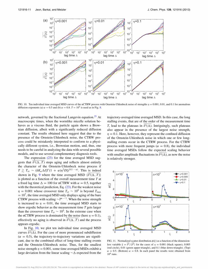
FIG. 11. Normalized scatter distribution φ(ξ ) as a function of the dimension-less variable ξ = δ2/〈δ2〉 for the cases of η = 0.001 (black square), 0.005(red circle), 0.01 (green upper-triangle), and 0.1 (blue down-triangle). (Top)α = 0.5. (Bottom) α = 0.8. In each panel the results were obtained from104 runs.

Downloaded 31 Aug 2013 to 129.128.216.34. This article is copyrighted as indicated in the abstract. Reuse of AIP content is subject to the terms at: http://jcp.aip.org/about/rights_and_permissions

121916-12 Jeon, Barkai, and Metzler J. Chem. Phys. 139, 121916 (2013)

FIG. 12. Dependence on the overall measurement time T of the normalizedscatter distribution φ(ξ ) for nCTRW process of anomalous exponent α = 0.5mixed with ηzOU(t) at η = 0.001 and 0.01. The distributions obtained fromthe nCTRW process with T = 107 are compared to the distributions from theone with T = 105.

C. Scatter distribution

Figure 11 illustrates the normalized scatter distribu-tion φ(ξ ) of the individual time averaged MSDs obtainedfrom 104 trajectories, as a function of the dimensionlessvariable ξ = δ2/〈δ2〉. The overall behavior is qualitativelyconsistent with those of the scatter distributions for addedBrownian noise, as shown in Fig. 5. The distribution becomes

increasingly ergodic as the Gaussian noise increases, espe-cially for the case of the more pronounced subdiffusive pro-cess (α = 0.5). Here, the finite contribution at ξ = 0 in φ(ξ )is gradually suppressed and the peak of the distributions isapproaching ξ = 1, as the strength of the noise is increased.

From the time averaged MSD (23) and its aging propertyin Fig. 9, it is also expected that the distribution attains ap-parent ergodic features as the observation time T is increased.We show this in Fig. 12 where the scatter distributions for thesame nCTRW process simulated up to T = 107 are comparedto the previous ones with T = 105. The general trend is thatφ(ξ ) becomes sharper as T increases. Importantly, this ergodiceffect becomes relevant provided that T is increased to at leastbe comparable with the crossover time Tcr ∼ (kKα�/[ (1+ α)η2D])1/(1 − α) defined above. As seen for the case for η

= 0.001, the distribution φ(ξ ) is almost unaffected, except atξ ≈ 0 where T � Tcr( ∼ 109). In contrast to this, the distribu-tion at η = 0.01 is noticeably narrower around ξ = 1 when Tis increased (Tcr ∼ 105).

D. p-variation test

In Fig. 13, we show the variation of the p-sums V(2/α)n (t)

and V (2)n (t) at increasing n for the simulated trajectories x(t)

of Fig. 7. For the smallest noise strength η = 0.001 shown inFig. 13, the p-variation test produces the result expected for

FIG. 13. Results of the p-variation test for nCTRW with superimposed Ornstein-Uhlenbeck noise ηzOU(t) for noise strengths η = 0.001, 0.01, and 0.1. Theupper and lower two rows are for α = 0.5 and 0.8. Same color codes as those of Fig. 6.

Downloaded 31 Aug 2013 to 129.128.216.34. This article is copyrighted as indicated in the abstract. Reuse of AIP content is subject to the terms at: http://jcp.aip.org/about/rights_and_permissions

121916-13 Jeon, Barkai, and Metzler J. Chem. Phys. 139, 121916 (2013)

the bare CTRW process. In the case of nCTRW with α = 0.8,this behavior persists in the presence of large noise strengthsup to η = 0.01. This is due to the fact that the bare CTRW pro-cess xα(t) features large displacements relative to those of theOrnstein-Uhlenbeck process. By contrast, for α = 0.5 the pro-files of V (2)

n (t) are mildly affected by the Ornstein-Uhlenbecknoise. Namely, the plateaus are tilted, with a somewhat largerslope at higher η, while their overall profiles preserve featuresof the monotonic, step-like behavior of the CTRW processxα(t).

Concurrently, we note that at larger values of η neitherV (2)

n (t) nor V(2/α)n (t) shows any indication of CTRW for both

α = 0.5 and 0.8. At these noise strengths, the Ornstein-Uhlenbeck noise dominates the p-variation results. As ex-plained in Sec. II B and shown in Fig. 1, in the limit n→ ∞ the p-sums for the Ornstein-Uhlenbeck noise con-verge to the results for Brownian noise. Thus, as V

(2/α)n (t)

rapidly decreases with increasing n in the case of Brown-ian noise, such a tendency is also present for the Ornstein-Uhlenbeck noise. Moreover, the spike-like profiles in V (4)

n (t)at n = 8 for η = 0.1 reflect the property of the Ornstein-Uhlenbeck noise (see Fig. 1). For p = 2, we find that thep-sum of the Ornstein-Uhlenbeck noise zOU(t) behaves asV (2)

n (t) ∼ 2Dk

[1 − exp(− k2

T2n )]( 2n

T)t (see the Appendix). This

result explains why V (2)n (t) monotonically increases with n

up to n ∼ log (kT)/log 2 ≈ 10, and for larger n it grows asV (2)

n (t) ∼ 2Dt , as shown in Fig. 13. As in the case of theabove nCTRW in the presence of Brownian noise zB(t), wefind that the p-variation result may be substantially affectedby the added Ornstein-Uhlenbeck noise, and the identificationof the underlying CTRW process becomes impossible.

VI. CONCLUSIONS

We introduced the noisy CTRW process, in which anordinary CTRW process is superimposed with Gaussiannoise, representing physically relevant cases when the pureCTRW motion becomes distorted by a noisy environment.We investigated how the additional ergodic noise interfereswith the non-ergodic behaviors of the underlying subdiffu-sive CTRW motion. Considering the two types of Gaussiannoises, Brownian noise and Ornstein-Uhlenbeck noise, wesimulated the resulting nCTRW motion and studied physi-cal quantities such as the ensemble and time averaged MSDs,the amplitude scatter distribution, and the behavior of thep-variation.

The analysis demonstrates that the influence of the Gaus-sian noise on these statistical quantities is highly specific tothe quantity of concern. Moreover, it depends not only on thetype of the noise and its strength but also on the length ofthe trajectory and the time scale. Depending on those spe-cific conditions, a quantitative analysis of the nCTRW pro-cess may reveal or mask the underlying non-ergodicity of thebare CTRW process. Thus, care is needed when we want todiagnose the stochastic nature of a physical process based onexperimental data. One way to avoid wrong conclusions is toapply complementary analysis techniques, such as the quan-tities used herein, or moment ratios, mean maximal excursion

methods, first passage dynamics, or others. The other neces-sary ingredient is a good physical intuition for the observedprocess. It would be also interesting to find analytical expres-sions for the p-variations, of mixed processes, as those wehave considered here. Our simulations results show that on fi-nite measurement time the noise is crucial, and could easilyprohibit our basic understanding of the underlying process.

From the present study, an experimentally relevant in-verse problem can be posed. Can one filter out the Gaus-sian noise from the experimentally obtained nCTRW pro-cess? Although obtaining the noise-cleansed profile from agiven nCTRW trajectory may appear infeasible, one could inprinciple obtain noise-free contributions in some ensemble-or time-averaged physical quantities of the nCTRW process,provided one is able to attain a sufficiently long trajectory. Inthe ensemble averaged MSD, the noise survives if the noiseis Brownian motion, while the CTRW process wins if thenoise is of Ornstein-Uhlenbeck type [see Eq. (22)]. This isof course what we expect, since the MSD of the Brownianmotion increases linearly with time, for CTRW like tα , andis a constant for Ornstein-Uhlenbeck—hence it is not sur-prising to see this behavior. In contrast, for the time aver-aged MSD, the dominant contribution comes always from thenoise [Eqs. (20) and (23)] in the sense that when the mea-surement time T is very large even the bounded Ornstein-Uhlenbeck noise wins over. This is due to an aging effect,the time averaged MSD of the CTRW process decreases withmeasurement time T. We thus see that the influence of thenoise on time averages is fundamentally different from thaton ensemble averages. As an example, one can extract almostsolely the noise contribution in the time-averaged MSD (andnot the bare CTRW itself) from a very long nCTRW trajec-tory. For an ergodic process this corresponds to the almostidentical noise contribution in the ensemble-averaged MSD,namely, η2〈z2(�)〉 � 〈δ2(�,T → ∞)〉. How to subtract thisnoise from real data is left for future work.

The nCTRW process developed herein is a physical ex-tension of pure CTRW dynamics. We believe that it representsan important advance in the truthful description of anomalousdiffusion data in thermal microscopic systems, where the en-vironment is noisy by definition and, for instance, will alsoinfluence molecular processes in biological cells.64 Mathe-matically, the nCTRW process is quite intuitive, due to theadditivity of the Gaussian noise.

Our present study can naturally be extended to more com-plicated noise sources, such as FBM, in order to obtain insightinto intracellular anomalous diffusion that shows both CTRWand FBM behaviors. It is expected that although FBM-likenoise should lead to similar effects on the statistical behaviorof the nCTRW process, the quantitative results will be pro-foundly different due to the scaling law of the FBM-like noise〈z2

FBM(t)〉 ∼ tα′with exponent 0 < α′ < 2.

ACKNOWLEDGMENTS

We acknowledge funding from the Academy of Finlandwithin the Finland Distinguished Professor (FiDiPro) schemeand from the Israel Science Foundation.

Downloaded 31 Aug 2013 to 129.128.216.34. This article is copyrighted as indicated in the abstract. Reuse of AIP content is subject to the terms at: http://jcp.aip.org/about/rights_and_permissions

121916-14 Jeon, Barkai, and Metzler J. Chem. Phys. 139, 121916 (2013)

APPENDIX: p-VARIATION OF CTRW SUBDIFFUSIONAND ORNSTEIN-UHLENBECK NOISE

We here discuss the p-variation properties of CTRW sub-diffusion and the Ornstein-Uhlenbeck noise in some moredetail.

1. CTRW subdiffusion

The subdiffusive CTRW process xα(t) with its PDF gov-erned by the fractional Fokker-Planck equation (8) can bedescribed through the subordinated Brownian motion xα(t)= B(Sα(t)), where B(τ ) defined with the internal time τ is anordinary Brownian motion satisfying 〈B(τ )〉 = 0 and 〈B2(τ )〉= 2Dτ . Here, Sα(t) is the so called inverse subordinatormatching the laboratory time t to the internal time τ . For theCTRW process xα(t), the p-sum V (2)

n (t) as n grows to infinitysatisfies57

V (2)(t) = 2DSα(t). (A1)

As shown in Fig. 1, Sα(t) has a step-like incremental pro-file and its jump times represent those for a given realiza-tion of CTRW process xα(t). On the other hand, the p-sumV

(2/α)n (t) (with 0 < α < 1) decreases with increasing n, fi-

nally V (2/α)(t) = 0 at n → ∞.57 This is also shown in thesimulations in Fig. 1.

2. Ornstein-Uhlenbeck noise

The ensemble average of the p-variation sum at finite nbecomes

⟨V (2)

n (t)⟩ ≈ 2D

k

[1 − exp

(−k

2

T

2n

)] (2n

T

)t, (A2)

neglecting an additional term which becomes negligible forlarge T. For small n � log (kT)/log 2, the above p sum simpli-fies to

⟨V (2)

n (t)⟩ ≈ 2D

k

2n

Tt. (A3)

In this case the linear slope of 〈V (2)(t)〉 increases with n upto values log (kT)/log 2 ∼ 10 (for the given parameter val-ues used in our simulation). This is shown in Fig. 1. In theother case, when n → ∞, the p sum converges to the re-sult of the Brownian noise 〈V (2)(t)〉 ≈ 2Dt . Hence, for largen � log (kT)/log 2, 〈V (2)(t)〉 is proportional to t with an n-independent slope. From the fact that on short-time scales (asn → ∞) the Ornstein-Uhlenbeck process behaves like a freeBrownian process, it can be inferred that its p-variation resultsare identical with those for simple Brownian motion. There-fore, V (4)(t) is expected to converge to zero as n increases.This is indeed observed in the simulations result in Fig. 1. Wefind that when n is small, the increment of V (4)(t) exhibitsa spike-like profile. This behavior presumably occurs dueto the fact that the quartic moment of the displacement x((j+ 1)T/[2n]) − x(jT/[2n]) becomes very small when the lagtime T/2n is larger than the relaxation time 1/k of the processfor small n.

1I. Y. Wong, M. L. Gardel, D. R. Reichman, E. R. Weeks, M. T.Valentine, A. R. Bausch, and D. A. Weitz, Phys. Rev. Lett. 92, 178101(2004).

2A. V. Weigel, B. Simon, M. M. Tamkun, and D. Krapf, Proc. Natl. Acad.Sci. U.S.A. 108, 6438 (2011).

3S. M. A. Tabei, S. Burov, H. Y. Kim, A. Kuznetsov, T. Huynh, J. Jureller,L. H. Philipson, A. R. Dinner, and N. F. Scherer, Proc. Natl. Acad. Sci.U.S.A. 110, 4911 (2013).

4J.-H. Jeon, V. Tejedor, S. Burov, E. Barkai, C. Selhuber-Unkel, K. Berg-Sørensen, L. Oddershede, and R. Metzler, Phys. Rev. Lett. 106, 048103(2011).

5E. Barkai, Y. Garini, and R. Metzler, Phys. Today 65(8), 29 (2012).6S. Havlin and D. Ben-Avraham, Adv. Phys. 36, 695 (1987).7J.-P. Bouchaud and A. Georges, Phys. Rep. 195, 127 (1990).8R. Metzler and J. Klafter, Phys. Rep. 339, 1 (2000).9R. Metzler and J. Klafter, J. Phys. A 37, R161 (2004).

10I. Golding and E. C. Cox, Phys. Rev. Lett. 96, 098102 (2006).11F. Höfling and T. Franosch, Rep. Prog. Phys. 76, 046602 (2013).12M. J. Saxton and K. Jacobson, Annu. Rev. Biophys. Biomol. Struct. 26,

373 (1997).13H. Scher and E. W. Montroll, Phys. Rev. B 12, 2455 (1975).14E. W. Montroll and G. H. Weiss, J. Math. Phys. 6, 167 (1965).15N. Leijnse, J.-H. Jeon, S. Loft, R. Metzler, and L. B. Oddershede, Eur.

Phys. J. Spec. Top. 204, 75 (2012).16H. Scher, G. Margolin, R. Metzler, J. Klafter, and B. Berkowitz, Geophys.

Res. Lett. 29, 1061, doi:10.1029/2001GL014123 (2002).17B. Berkowitz, A. Cortis, M. Dentz, and H. Scher, Rev. Geophys. 44,

RG2003, doi:10.1029/2005RG000178 (2006).18C. Monthus and J.-P. Bouchaud, J. Phys. A 29, 3847 (1996).19S. Burov and E. Barkai, Phys. Rev. Lett. 98, 250601 (2007).20R. Metzler, E. Barkai, and J. Klafter, Phys. Rev. Lett. 82, 3563 (1999);

Europhys. Lett. 46, 431 (1999).21I. Nordlund, Z. Phys. Chem. 87, 40 (1914).22C. Bräuchle, D. C. Lamb, and J. Michaelis, Single Particle Tracking

and Single Molecule Energy Transfer (Wiley-VCH, Weinheim, Germany,2012); X. S. Xie, P. J. Choi, G.-W. Li, N. K. Lee, and G. Lia, Annu. Rev.Biophys. 37, 417 (2008).

23I. Bronstein, Y. Israel, E. Kepten, S. Mai, Y. Shav-Tal, E. Barkai, and Y.Garini, Phys. Rev. Lett. 103, 018102 (2009).

24J. Szymanski and M. Weiss, Phys. Rev. Lett. 103, 038102 (2009).25J.-H. Jeon, N. Leijnse, L. B. Oddershede, and R. Metzler, New J. Phys. 15,

045011 (2013).26A. Caspi, R. Granek, and M. Elbaum, Phys. Rev. Lett. 85, 5655

(2000).27D. Banks and C. Fradin, Biophys. J. 89, 2960 (2005).28E. Kepten, I. Bronshtein, and Y. Garini, Phys. Rev. E 87, 052713 (2013).29S. C. Weber, A. J. Spakowitz, and J. A. Theriot, Phys. Rev. Lett. 104,

238102 (2010).30S. Burov, J.-H. Jeon, R. Metzler, and E. Barkai, Phys. Chem. Chem. Phys.

13, 1800 (2011).31Y. Meroz, I. Eliazar, and J. Klafter, J. Phys. A 42, 434012 (2009); Y. Meroz,

I. M. Sokolov, and J. Klafter, Phys. Rev. Lett. 110, 090601 (2013).32W. Deng and E. Barkai, Phys. Rev. E 79, 011112 (2009).33J.-H. Jeon and R. Metzler, Phys. Rev. E 81, 021103 (2010). Note, how-

ever, the occurrence of transient non-ergodic relaxation to equilibrium un-der confinement, as shown in J.-H. Jeon and R. Metzler, Phys. Rev. E 85,021147 (2012).

34I. Goychuk, Phys. Rev. E 80, 046125 (2009); Adv. Chem. Phys. 150, 187(2012).

35A. Fulinski, Phys. Rev. E 83, 061140 (2011).36G. R. Kneller, K. Baczynski, and M. Pasenkiewicz-Gierula, J. Chem. Phys.

135, 141105 (2011).37J.-H. Jeon, H. M.-S. Monne, M. Javanainen, and R. Metzler, Phys. Rev.

Lett. 109, 188103 (2012).38G. Zumofen and J. Klafter, Physica D 69, 436 (1993).39A. Godec and R. Metzler, Phys. Rev. Lett. 110, 020603 (2013).40D. Froemberg and E. Barkai, Phys. Rev. E 87, 031104(R) (2013).41J.-P. Bouchaud, J. Phys. (Paris) 2, 1705 (1992).42G. Bel, and E. Barkai, Phys. Rev. Lett. 94, 240602 (2005); A. Rebenshtok

and E. Barkai, ibid. 99, 210601 (2007).43M. A. Lomholt, I. M. Zaid, and R. Metzler, Phys. Rev. Lett. 98, 200603

(2007).44Y. He, S. Burov, R. Metzler, and E. Barkai, Phys. Rev. Lett. 101, 058101

(2008).

Downloaded 31 Aug 2013 to 129.128.216.34. This article is copyrighted as indicated in the abstract. Reuse of AIP content is subject to the terms at: http://jcp.aip.org/about/rights_and_permissions

121916-15 Jeon, Barkai, and Metzler J. Chem. Phys. 139, 121916 (2013)

45A. Lubelski, I. M. Sokolov, and J. Klafter, Phys. Rev. Lett. 100, 250602(2008).

46J. H. P. Schulz, E. Barkai, and R. Metzler, Phys. Rev. Lett. 110, 020602(2013); E. Barkai, ibid. 90, 104101 (2003).

47S. Burov, R. Metzler, and E. Barkai, Proc. Natl. Acad. Sci. U.S.A. 107,13228 (2010).

48T. Neusius, I. M. Sokolov, and J. C. Smith, Phys. Rev. E 80, 011109 (2009).49I. M. Sokolov, E. Heinsalu, P. Hänggi, and I. Goychuk, Europhys. Lett. 86,

30009 (2009).50T. Miyaguchi and T. Akimoto, Phys. Rev. E 87, 032130 (2013).51M. J. Saxton, Biophys. J. 72, 1744 (1997).52A. Caspi, R. Granek, and M. Elbaum, Phys. Rev. E 66, 011916 (2002).53T. Akimoto, Phys. Rev. Lett. 108, 164101 (2012).54S. Condamin, V. Tejedor, R. Voituriez, O. Bénichou, and J. Klafter, Proc.

Natl. Acad. Sci. U.S.A. 105, 5675 (2008).55V. Tejedor, O. Bénichou, R. Voituriez, R. Jungmann, F. Simmel, C.

Selhuber-Unkel, L. Oddershede, and R. Metzler, Biophys. J. 98, 1364(2010).

56M. Bauer, R. Valiullin, G. Radons, and J. Kaerger, J. Chem. Phys. 135,144118 (2011).

57M. Magdziarz, A. Weron, K. Burnecki, and J. Klafter, Phys. Rev. Lett.103, 180602 (2009); M. Magdziarz and J. Klafter, Phys. Rev. E 82, 011129(2010).

58K. Burnecki, E. Kepten, J. Janczura, I. Bronshtein, Y. Garini, and A. Weron,Biophys. J. 103, 1839 (2012).

59J.-H. Jeon and R. Metzler, J. Phys. A: Math. Theor. 43, 252001(2010).

60E. Barkai, R. Metzler, and J. Klafter, Phys. Rev. E 61, 132 (2000). Note theoccurrence of the factor (1 − α) here due to the different choice of ψ(t)in Eq. (15).

61C. A. Dreiss, Soft Matter 3, 956 (2007).62J. Galvan-Miyoshi, J. Delgado, and R. Castillo, Eur. Phys. J. E 26, 369

(2008).63M. Bellour, M. Skouri, J.-P. Munch, and P. Hébraud, Eur. Phys. J. E 8, 431

(2002).64S. Eule and R. Friedrich, Phys. Rev. E 87, 032162 (2013).

Downloaded 31 Aug 2013 to 129.128.216.34. This article is copyrighted as indicated in the abstract. Reuse of AIP content is subject to the terms at: http://jcp.aip.org/about/rights_and_permissions