arX

iv:m

ath/

0509

257v

2 [

mat

h.PR

] 3

0 Ju

n 20

06

The Annals of Probability

2006, Vol. 34, No. 3, 987–1011DOI: 10.1214/009117906000000052c© Institute of Mathematical Statistics, 2006

CARNE–VAROPOULOS BOUNDS FOR CENTERED

RANDOM WALKS

By Pierre Mathieu

CMI

We extend the Carne–Varopoulos upper bound on the probabilitytransitions of a Markov chain to a certain class of nonreversible pro-cesses by introducing the definition of a “centering measure.” In thecase of random walks on a group, we study the connections betweendifferent notions of centering.

1. Introduction. Let X = (Xt, t ∈ N) be a Markov chain taking its valuesin some discrete set, V .

The paper is concerned with two related issues: in Section 2, the statespace of the Markov chain is not assumed to have any special algebraicstructure. We introduce a “centering condition” which generalizes the clas-sical reversibility assumption. The main result is an extension of the Carne–Varopoulos inequality for the transition probabilities of a not necessarilyreversible Markov chain; see Theorems 2.8 and 2.10. In Section 3 we restrictour attention to random walks on groups. We then investigate the relationbetween different possible definitions of a “centered random walk.”

The initial motivation of this work was to find a different, more geometri-cal and combinatorial interpretation of the bounds obtained by Alexopoulosfor random walks on nilpotent groups; see [1]. This is partially achieved, asfar as the upper bound is concerned, in Proposition 3.3(a). But it turned outthat our notion of centering measure can also be used to study nonreversiblerandom walks on other examples of groups, such as Baumslag Solitar groupsor wreath products; see Section 3.

The Carne–Varopoulos bound. A measure, π, on V is called reversible forthe Markov chain X if the following detailed balance condition is satisfied:

Received June 2004; revised July 2005.AMS 2000 subject classification. 60J10.Key words and phrases. Centered Markov chains, random walks, Carne–Varopoulos

bounds, Poisson boundary.

This is an electronic reprint of the original article published by theInstitute of Mathematical Statistics in The Annals of Probability,2006, Vol. 34, No. 3, 987–1011. This reprint differs from the original in paginationand typographic detail.

1

2 P. MATHIEU

for all x, y ∈ V ,

π(x)P[X1 = y|X0 = x] = π(y)P[X1 = x|X0 = y].(1)

Not all Markov chains admit a reversible measure.The detailed balance condition is equivalent to saying that the transition

operator of X is symmetric in L2(V,π). It is then possible to apply differenttools from analysis, in particular spectral theory, to study the Markov chain.As an example of a distinguished property of reversible Markov chains, letus quote the Carne–Varopoulos upper bound: assume that π is a reversiblemeasure for X ; then, for all x, y ∈ V and t ∈ N

∗, we have

P[Xt = y|X0 = x]≤ 2

√

π(y)

π(x)e−d2(x,y)/(2t).(2)

In (2), d(x, y) is the natural distance associated to X , that is, the minimalnumber of steps required for the Markov chain to go from x to y. The firstpaper to deal with such long-range estimates for transition probabilities is[11]. We refer to [3] or [13], Theorem 14.12 and Lemma 14.21 for a proof of(2) which relies on spectral theory. Inequality (2) gives a crude upper boundon the tail of the law of Xt which turned out to be very useful in the analysisof the long-time behavior of reversible Markov chains.

Centered random walks on a graph. This paper arose as an attempt toget a similar bound for a not necessarily reversible Markov chain. Thus wedo not assume that X admits a reversible measure and ask: does there exista constant C such that, for all x, y ∈ V and t ∈ N

∗,

P[Xt = y|X0 = x]≤ Ce−d2(x,y)/(Ct)?(3)

In the case of random walks in Zd, that is, if Xt is obtained as a sum of

t independent, identically distributed random variables with finite supportin Z

d, then inequality (3) holds if and only if the mean value of X1 vanishesor, equivalently, E[Xt] = 0 for all t ∈ N. By analogy, we interpret (3) as acentering condition for the Markov chain X although, for a general set V ,it does not make sense anymore to speak of “vanishing mean” for X1.

The transition probabilities of X endow its state space V with a structureof weighted oriented graph. In the second part of the paper, we define theclass of centered Markov chains in terms of a splitting on this graph intooriented cycles; see Definition 2.1. Markov chains admitting a reversiblemeasure are centered. We then prove a Carne–Varopoulos upper bound ofthe form (3) in Theorem 2.8. We also prove that the Dirichlet form satisfiesa sector condition and derive some easy consequences in terms of Greenkernels; see Lemma 2.12 and Proposition 2.13. In order to illustrate ourdefinition, a special case of our general result is described at the end of thisintroduction.

CENTERED RANDOM WALKS 3

Centered random walks on a group. The third part of the paper is de-voted to random walks on groups. That is, we assume that V is a discretegroup; choose a finite generating set for V , say G and define Xt as a sumof independent, uniformly distributed random variables on G. Let µ be theuniform probability distribution on G, and let µt denote the tth convolutionpower of µ. Thus µt is the law of Xt. In this context, (3) reads: does thereexist a constant C such that, for all x ∈ V and t ∈ N

∗,

µt(x) ≤ Ce−d2(id ,y)/(Ct)?(4)

Here id is the unit element in V . d(x, y) is the word distance between x andy. Up to multiplicative constants, d(x, y) is independent of the choice of thegenerating set.

The graph associated to the random walk X is now a Cayley graph ofV , but, unless G is symmetric, this is an oriented Cayley graph. Findingcycles in this Cayley graph amounts to writing id as a product of elementsof G. We may apply results of the second part to derive sufficient conditionson G that imply (4): let N be the semigroup made of the elements of Vthat can be written as products of elements in G where each of the elementsof G appears the same number of times. In Proposition 3.1, we show thatif id ∈ N , then (4) is satisfied for some constant C. One can also considersums of independent, identically distributed random variables with a moregeneral law than the uniform distribution over G.

Checking whether id ∈ N is an—apparently new—combinatorial prob-lem involving the geometry of V and the choice of G. We solve it for nilpo-tent groups. Baumslag–Solitar groups, examples of wreath products and freegroups are also considered; see Section 3.3.

As a consequence, in the above mentioned examples, we obtain the equiv-alence of the following two centering conditions:

(C1) id ∈N ;(C2) the image of the uniform measure on G by any homomorphism of V

on R has vanishing mean.

Application to the rate of escape. Carne–Varopoulos bounds can be usedin order to bound the rate of escape of the random walk from its initialpoint. In the case of a centered Markov chain, it is easy to deduce fromthe Carne–Varopoulos bound that the rate of escape vanishes if the volumegrowth is subexponential; see Theorem 2.11. In the case of random walkson a group, one can do much better and prove that the speed vanishes ifand only if the Poisson boundary is trivial; see Proposition 3.11. This laststatement extends well-known results for symmetric random walks; see [5, 9]or [12], among other references.

4 P. MATHIEU

An example. We consider the special case of a Markov chain associated toan oriented unweighted graph structure on V . So let E ⊂ V ×V be such that,for all x ∈ V , the number of points y ∈ V such that (x, y) ∈ E is finite anduniformly bounded in x. The Markov process (Xt, t ∈ N) is defined by theusual rule: at each step, one selects at random (with uniform distribution)one of the edges in E starting from the current position. Then the randomwalker jumps along the chosen edge.

A cycle is a sequence γ = (x0, x1, . . . , xk) in V such that xk = x0 and(xi, xi+1) ∈ E for all i = 0, . . . , (k − 1). We allow cycles of the form (x0, x0)or (x0, x1, x0). Let |γ| = k be the length of γ. We write that the edge (x, y)belongs to γ if, for some i, we have x = xi and y = xi+1.

Assume that there exists a collection of cycles, (γi, i ∈ N), satisfying thefollowing two properties: (i) supi |γi| < ∞, (ii) any edge (x, y) ∈ E belongsto exactly one of the γi’s; then (3) holds for some constant C.

Now suppose that V is a group with generating set G = (g1, . . . , gK).Then E = {(x, y) :x−1y ∈ G} defines an oriented Cayley graph on V . Cyclescorrespond to relations in V . Conditions (i) and (ii) are satisfied if there is apermutation of {1, . . . ,K}, say σ, such that gσ(1) · gσ(2) · · ·gσ(K) = id . Then(4) is satisfied.

The condition gσ(1) · gσ(2) · · ·gσ(K) = id obviously implies that, for any

homomorphism h of V on R,∑K

i=1 h(gi) = 0. Whether the converse is trueor not depends on the group; see Section 3.

Further references. The idea of using a decomposition of the state spaceof a Markov chain into cycles is not new. We refer in particular to the workof Kalpazidou [10] and to the first chapters of the book [7]. However, theseauthors are mostly interested in recurrent Markov chains.

The main technical tools used to prove our main result, Theorem 2.8, areborrowed from the work of Hebisch and Saloff-Coste, although some extrawork is necessary to handle the lack of reversibility.

Comparison theorems for Green kernels similar to our Proposition 2.13(i)have been obtained by various authors; see, for instance, [2] or [4].

2. Centered Markov chains on graphs.

2.1. Definitions. In this section we introduce the definitions related tothe graph structure induced by a Markov chain on its state space. As in theIntroduction, let (Xt, t ∈ N) be a Markov chain taking its values in someinfinite countable set, V . We assume that X is irreducible.

For x and y in V , define q(x, y) = P[X1 = y|X0 = x]. Considering q(x, y)as the weight of the edge (x, y) ∈ V ×V , we can see Γ = (V, q) as a weighted,oriented graph.

CENTERED RANDOM WALKS 5

Call a cycle a finite sequence γ = (x0, x1, . . . , xk) of points in V suchthat xk = x0 and q(xi, xi+1) > 0 for all i = 0, . . . , (k − 1). We allow cycles ofthe form (x0, x0) or (x0, x1, x0). Sometimes we identify the cycle γ with asequence of edges, that is, γ = ((x0, x1), . . . , (xk−1, xk)). Define |γ| = k to bethe length of γ. We further suppose that cycles are edge self-avoiding, thatis, that (xi, xi+1) = (xj , xj+1) implies that i = j. But we do not assume thatcycles are vertex self-avoiding.

Definition 2.1. Let m be a measure on V . The graph Γ is centered ifthere is a collection of cycles (γi, i ∈ N) and positive weights (qi, i ∈ N) suchthat:

(i) supi |γi|< ∞,(ii) for any x, y ∈ V , we have

m(x)q(x, y) =∑

i

qi1(x,y)∈γi.(5)

We then call m a centering measure for the process (Xt) (or for the graphΓ).

To avoid empty statements, we shall always assume that m is not identi-cally vanishing. From Remark 2.6 below it will follow that m(x) > 0 for allx ∈ V .

We shall use the notation ε = infx∈V m(x) ≥ 0 and C0 = supi |γi|.

Remark 2.2. We may suppress the condition that cycles have to beedge self-avoiding. Let us call “generalized cycle” a sequence satisfying allthe properties of cycles except it may have edge self-intersections. For a givenedge, (x, y) ∈ V × V , let N((x, y), γ) = #{e ∈ γ : (x, y) = e} be the numberof occurrences of (x, y) in the generalized cycle γ.

Γ is then centered iff there exists a collection of generalized cycles, (γi, i ∈N), such that supi |γi|< ∞ and, for all x, y ∈ V , we have

m(x)q(x, y) =∑

i

qiN((x, y), γi).(6)

This fact is easy to prove by splitting generalized cycles into edge self-avoiding cycles.

Remark 2.3 (The reversible case). Suppose that m is a reversible mea-sure for X , that is, assume that the detailed balance condition is satisfied:for any x, y ∈ V ,

m(x)q(x, y) = m(y)q(y,x).

6 P. MATHIEU

Choose cycles of the form γ = (x, y,x) whenever q(x, y) > 0 and γ = (x,x)whenever q(x,x) > 0. To the cycle (x, y,x), we attach the weight q = m(x)q(x, y);to the cycle (x,x), we attach the weight q = m(x)q(x,x). It is then immedi-ate to deduce from the detailed balance condition that condition (5) holds.In other words, reversible graphs are centered.

Example 2.4 (Unweighted graphs). Let E ⊂ V × V . Assume that, forall y ∈ V , the number of points x ∈ V such that (x, y) ∈ E is finite. LetN+(x) = {y ∈ V : (x, y) ∈ E}, and define

q(x, y) =

1

#N+(x), if (x, y) ∈ E,

0, otherwise,

so that the random walker moves by choosing uniformly at random an edgein E starting from its current position and then jumping along the chosenedge. Let m(x) = #N+(x).

Assume that there exists a collection of cycles, (γi, i ∈ N), and an integer,n, such that (i) supi |γi|< ∞, and (ii) for any edge e ∈E, #{i : e ∈ γi}= n.Then Γ is centered.

Proof. Indeed we have∑

i

1(x,y)∈γi= n = nm(x)q(x, y),

for any edge (x, y) ∈ E. Thus we may choose the weights qi = 1n to check

condition (5). �

Note that, for Γ to be centered for the measure m, it is necessary that#{y ∈ V : (y,x) ∈E} = #{y ∈ V : (x, y) ∈ E} for all x ∈ V .

Lemma 2.5. Let Γ be centered for m. Then m is an invariant measurefor X, that is, for all y ∈ V , one has

∑

x∈V m(x)q(x, y) = m(y).

Proof. For given x ∈ V and i ∈ N, note that there exists y ∈ V with(x, y) ∈ γi iff there exists y ∈ V with (y,x) ∈ γi. Because cycles are edgeself-avoiding, #{y ∈ V : (x, y) ∈ γi} = #{y ∈ V : (y,x) ∈ γi}. Therefore

∑

y

∑

i

qi1(x,y)∈γi=∑

y

∑

i

qi1(y,x)∈γi.

Thus∑

x

m(x)q(x, y) =∑

x

∑

i

qi1(x,y)∈γi

CENTERED RANDOM WALKS 7

=∑

x

∑

i

qi1(y,x)∈γi

=∑

x

m(y)q(y,x) = m(y).�

Remark 2.6. As a consequence of the lemma, since we have assumedthat X is irreducible, we must have m(x) > 0 for all x ∈ V . Keeping in mindthat the weights qi are positive, we note that it implies that, for any x, y ∈ V ,q(x, y) > 0 if and only if there exists at least one i ∈ N such that (x, y) ∈ γi.

We now recall the definition of the distance associated to Γ. For x, y ∈ V ,let d(x, y) be the smallest k ∈ N such that there is a sequence x0, . . . , xk

with x0 = x, xk = y and q(xi, xi+1)+ q(xi+1, xi) > 0. In other words, d is theclassical graph distance associated to the undirected graph structure on Vdefined by

E0 = {(x, y) ∈ V × V : q(x, y) + q(y,x) > 0}.

Remark 2.7. Assume that Γ is centered. If d(x, y) = k, then there existsa sequence (x0, . . . , xK) such that x0 = x, xK = y and q(xi, xi+1) > 0, for alli. Besides we may choose K ≤C0k.

Indeed, if d(x, y) = 1, then, either q(x, y) > 0—and then K = 1—orq(x, y) = 0, in which case q(y,x) > 0. In the latter case, we choose one cycle γi

such that (y,x) ∈ γi, say γi = (y,x,x2, . . . , xa−1, y). Then a≤ C0. Besides wehave found a path, (x,x2, . . . , xa−1, y), of length bounded by a≤ C0, linkingx to y and such that q(e1, e2) > 0 when (e1, e2) ∈ γi. Thus the claim is provedfor k = 1. The general case follows.

We can now state the main result of this section:

Theorem 2.8. Let Γ be a centered graph for the measure m. Assumethat ε = infx∈V m(x) > 0. Then there exists a constant C, that only dependson ε and C0, such that, for all x, y ∈ V and t ∈ N

∗, we have

P[Xt = y|X0 = x] ≤Cm(y)e−d2(x,y)/(Ct).

2.2. Proof of Theorem 2.8.

Preliminaries on Dirichlet forms. Define the operator Qf(x) = E[f(X1)|X0 = x] =

∑

y∈V q(x, y)f(y) on functions with finite support. Qt will denotethe tth power of Q.

8 P. MATHIEU

Let Q∗ be the adjoint of Q with respect to the measure m. Then Q∗f(x) =∑

y∈V q∗(x, y)f(y), with q∗(y,x) = m(x)m(y) q(x, y). Using (5), we get that

q∗(y,x)m(y) =∑

i

qi1(x,y)∈γi.

This last formula may as well be written

q∗(x, y)m(x) =∑

i

qi1(x,y)∈γ∗i,

where, for a cycle γ, we use the notation γ∗ to denote the reversed cycle.(Reverse the order of the sequence defining γ.) Thus the graph Γ∗ = (V, q∗)is also centered for the same measure m. It is actually the graph associatedto the time reversal of the Markov chain X . In particular all the results weare about to prove for centered graphs may be applied to Γ∗.

We have already noticed that m(Qf) = m(f). The operator Q beingpositivity preserving, we thus have m(|Qf |) ≤ m(|f |). It is also clear thatsupx∈V |Qf(x)| ≤ supx∈V |f(x)|. It follows from Jensen’s inequality, or by in-terpolation, that Q is a contraction in Lp(V,m) for all p ∈ [1,∞]. By duality,Q∗ is also a contraction in Lp(V,m).

Define the Dirichlet form E(f, g) = m(g·(I − Q)f). It can be expressed

with the kernel q by

E(f, g) =∑

x,y∈V

m(x)q(x, y)g(x)(f(x)− f(y)).

We also consider the symmetrized Dirichlet form

E0(f, g) =1

2(E(f, g) + E(g, f))

= m

(

g·

(

I −Q + Q∗

2

)

f

)

=∑

x,y∈V

m(x)q(x, y) + q∗(x, y)

2g(x)(f(x)− f(y)).

Since, m(x)(q(x, y) + q∗(x, y)) = m(x)q(x, y) + m(y)q(y,x), we have

E0(f, g) = 12

∑

x,y∈V

p0(x, y)(f(x)− f(y))(g(x)− g(y)),(7)

with

p0(x, y) = p0(y,x) = 12(m(x)q(x, y) + m(y)q(y,x)).(8)

CENTERED RANDOM WALKS 9

Let us now compute the antisymmetric part of E :

E(f, g)−E0(f, g) = m

(

g·

Q∗ −Q

2f

)

=∑

x,y∈V

m(x)g(x)f(y)q∗(x, y)− q(x, y)

2

=1

2

∑

x,y∈V

(f(x)g(y)− f(y)g(x))m(x)q(x, y).

And, using (5), we obtain the useful representation formula:

E(f, g)−E0(f, g) = 12

∑

i

qi

∑

(x,y)∈γi

(f(x)g(y)− f(y)g(x)).(9)

Poincare inequality. We shall use the following Poincare inequality onthe discrete circle: let γ be a cycle. There exists a constant, Cγ , such that,for all functions g such that

∑

x∈γ g(x) = 0, we have∑

x∈γ

g(x)2 ≤Cγ

∑

(x,y)∈γ

(g(x)− g(y))2.(10)

The best constant in (10) is the inverse spectral gap of the nearest-neighborsymmetric random walk on γ; thus (10) is a Poincare inequality. Besides,the constant Cγ depends only on the length |γ|.

Proof of Theorem 2.8. The “symmetric” version of Theorem 2.8 isstated as Theorem 14.12 in [13]. (The argument is due to Hebish and Saloff-Coste; see [6].) We try to follow Woess as closely as possible, starting withthe next lemma, but there is an extra nonsymmetric term to be handled byspecific arguments. This is where the assumption (5) enters into play.

Keep in mind that C is a constant which is allowed to depend only onε and C0. Choose some reference point o ∈ V . For s ∈ R, define the functionws(x) = esd(o,x). We need the following.

Lemma 2.9. There exists a constant C, that depends on C0 only, andsuch that, for all s ∈ R, |s| ≤ 1

C , and for any function f with finite support,we have

E(wsf,w−sf)≥−Cs2(1 + eC|s|)m(f2).

Proof. We use the notation w = ws and note that, replacing f withwf , we have to prove that

E(w2f, f)≥−Cs2(1 + eC|s|)m(w2f2).

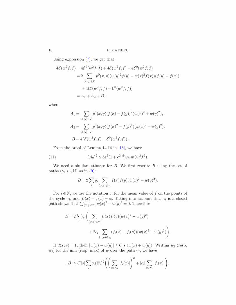
10 P. MATHIEU

Using expression (7), we get that

4E(w2f, f) = 4E0(w2f, f) + 4E(w2f, f)− 4E0(w2f, f)

= 2∑

(x,y)∈V

p0(x, y)(w(y)2f(y)−w(x)2f(x))(f(y)− f(x))

+ 4(E(w2f, f)− E0(w2f, f))

= A1 + A2 + B,

where

A1 =∑

(x,y)∈V

p0(x, y)(f(x)− f(y))2(w(x)2 + w(y)2),

A2 =∑

(x,y)∈V

p0(x, y)(f(x)2 − f(y)2)(w(x)2 −w(y)2),

B = 4(E(w2f, f)− E0(w2f, f)).

From the proof of Lemma 14.14 in [13], we have

(A2)2 ≤ 8s2(1 + e2|s|)A1m(w2f2).(11)

We need a similar estimate for B. We first rewrite B using the set ofpaths (γi, i ∈ N) as in (9):

B = 2∑

i

qi

∑

(x,y)∈γi

f(x)f(y)(w(x)2 −w(y)2).

For i ∈ N, we use the notation ci for the mean value of f on the points ofthe cycle γi, and fi(x) = f(x) − ci. Taking into account that γi is a closedpath shows that

∑

(x,y)∈γiw(x)2 −w(y)2 = 0. Therefore

B = 2∑

i

qi

(

∑

(x,y)∈γi

fi(x)fi(y)(w(x)2 −w(y)2)

+ 2ci

∑

(x,y)∈γi

(fi(x) + fi(y))(w(x)2 −w(y)2)

)

.

If d(x, y) = 1, then |w(x) −w(y)| ≤ C|s|(w(x) + w(y)). Writing wi (resp.wi) for the min (resp. max) of w over the path γi, we have

|B| ≤C|s|∑

i

qi(wi)2

((

∑

x∈γi

|fi(x)|

)2

+ |ci|∑

x∈γi

|fi(x)|

)

.

CENTERED RANDOM WALKS 11

We now use the Poincare inequality (10) for the function fi to deducethat

(

∑

x∈γi

|fi(x)|

)2

≤ |γi|∑

x∈γi

(fi(x))2 ≤ Cγi|γi|

∑

(x,y)∈γi

(fi(x)− fi(y))2

= Cγi|γi|

∑

(x,y)∈γi

(f(x)− f(y))2.

The length of γi being bounded by C0, we may therefore choose a constantC, independent of i, such that

(

∑

x∈γi

|fi(x)|

)2

≤C∑

(x,y)∈γi

(f(x)− f(y))2.

Also note that (ci)2 ≤C

∑

x∈γif2(x).

From the previous inequalities, we conclude that

|B| ≤ C|s|∑

i

qi(wi)2

(

∑

(x,y)∈γi

(f(x)− f(y))2

+

√

∑

x∈γi

f2(x)√

∑

(x,y)∈γi

(f(x)− f(y))2)

.

For the next step, we use the fact that w is roughly constant on each pathγi. More precisely, since |γi| ≤ C0, two points on γi are at distance at mostC0. Therefore wi ≤ eC|s|wi, where C depends only on C0. Therefore

|B| ≤ C|s|eC|s|∑

i

qi

(

∑

(x,y)∈γi

(f(x)− f(y))2(w(x)2 + w(y)2)

+

√

∑

x∈γi

f2(x)w(x)2

×√

∑

(x,y)∈γi

(f(x)− f(y))2(w(x)2 + w(y)2)

)

≤ C|s|eC|s|

(

∑

i

qi

∑

(x,y)∈γi

(f(x)− f(y))2(w(x)2 + w(y)2)

+

√

∑

i

qi

∑

x∈γi

f2(x)w(x)2

×√

∑

i

qi

∑

(x,y)∈γi

(f(x)− f(y))2(w(x)2 + w(y)2)

)

,

12 P. MATHIEU

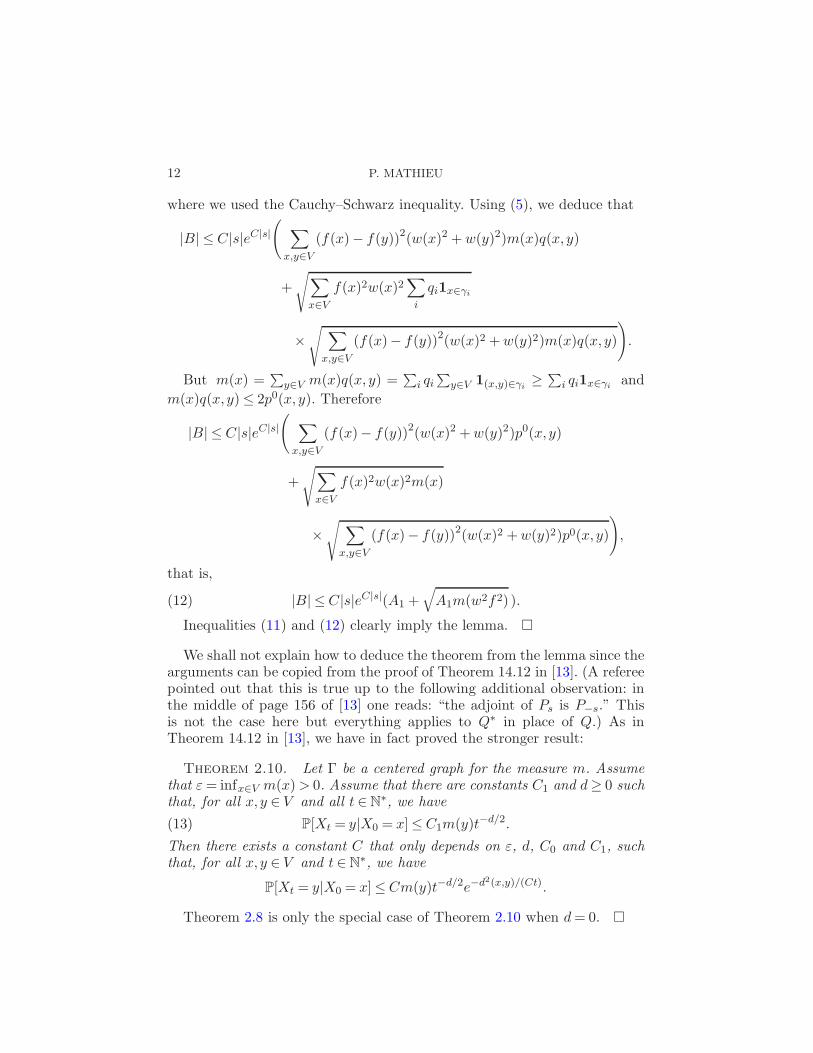
where we used the Cauchy–Schwarz inequality. Using (5), we deduce that

|B| ≤ C|s|eC|s|

(

∑

x,y∈V

(f(x)− f(y))2(w(x)2 + w(y)2)m(x)q(x, y)

+

√

∑

x∈V

f(x)2w(x)2∑

i

qi1x∈γi

×√

∑

x,y∈V

(f(x)− f(y))2(w(x)2 + w(y)2)m(x)q(x, y)

)

.

But m(x) =∑

y∈V m(x)q(x, y) =∑

i qi∑

y∈V 1(x,y)∈γi≥∑

i qi1x∈γiand

m(x)q(x, y) ≤ 2p0(x, y). Therefore

|B| ≤ C|s|eC|s|

(

∑

x,y∈V

(f(x)− f(y))2(w(x)2 + w(y)2)p0(x, y)

+

√

∑

x∈V

f(x)2w(x)2m(x)

×√

∑

x,y∈V

(f(x)− f(y))2(w(x)2 + w(y)2)p0(x, y)

)

,

that is,

|B| ≤ C|s|eC|s|(A1 +√

A1m(w2f2) ).(12)

Inequalities (11) and (12) clearly imply the lemma. �

We shall not explain how to deduce the theorem from the lemma since thearguments can be copied from the proof of Theorem 14.12 in [13]. (A refereepointed out that this is true up to the following additional observation: inthe middle of page 156 of [13] one reads: “the adjoint of Ps is P−s.” Thisis not the case here but everything applies to Q∗ in place of Q.) As inTheorem 14.12 in [13], we have in fact proved the stronger result:

Theorem 2.10. Let Γ be a centered graph for the measure m. Assumethat ε = infx∈V m(x) > 0. Assume that there are constants C1 and d≥ 0 suchthat, for all x, y ∈ V and all t ∈ N

∗, we have

P[Xt = y|X0 = x]≤ C1m(y)t−d/2.(13)

Then there exists a constant C that only depends on ε, d, C0 and C1, suchthat, for all x, y ∈ V and t ∈ N

∗, we have

P[Xt = y|X0 = x]≤ Cm(y)t−d/2e−d2(x,y)/(Ct).

Theorem 2.8 is only the special case of Theorem 2.10 when d = 0. �

CENTERED RANDOM WALKS 13

2.3. Rate of escape. The next statement is an easy consequence of theCarne–Varopoulos bounds.

Theorem 2.11. Assume that Γ is centered for a measure m such thatε = infx∈V m(x) > 0. Let V (t) = ♯{x ∈ V :d(o,x) ≤ t} be the volume of theball centered at o. (o is an arbitrary reference point.) If lim supt→∞

1t logV (t) =

0, then for all α > 0, we have

limt→+∞

P[d(o,Xt)≥ αt|X0 = o] = 0.

Proof. Use Theorem 2.8 and the fact that d(o,Xt)≤ t if X0 = o, to getthat

P[d(o,Xt)≥ αt|X0 = o] =∑

x;αt≤d(o,x)≤t

P[Xt = x|X0 = o]

≤∑

x;αt≤d(o,x)≤t

Ce−d2(o,x)/(Ct)

≤ Ce−α2t/CV (t) → 0. �

2.4. Sector condition and Green kernels.

Lemma 2.12 (Sector condition). Let Γ be a centered graph for the mea-sure m. There exists a constant M , function of C0 only, such that, for allfinitely supported functions f and g, we have

E(f, g)2 ≤ M2E(f, f)E(g, g).

Proof. We write that E(f, g) = E0(f, g) + E(f, g) − E0(f, g), where, asbefore, E0(f, g) = 1

2(E(f, g) + E(g, f)) is the symmetric part of E .Since E0 is a symmetric bilinear form, we have E0(f, g)2 ≤ E0(f, f)E0(g, g) =

E(f, f)E(g, g). It remains to prove that (E(f, g)−E0(f, g))2 ≤M2E(f, f)E(g, g).From (9), we know that

E(f, g)−E0(f, g) = 12

∑

i

qi

∑

(x,y)∈γi

(f(x)g(y)− f(y)g(x)).

Note that the quantity∑

(x,y)∈γi(f(x)g(y)−f(y)g(x)) remains unchanged

if we modify by a constant the value of f or g on γi. Thus let ci (resp. di) bethe mean of f (resp. g) on γi and set fi = f − ci (resp. gi = g−di). From thePoincare inequality (10), we get a constant Mi, that depends on the lengthof γi only, such that

∑

x∈γi

f2i (x) ≤ Mi

∑

(x,y)∈γi

(f(x)− f(y))2,

∑

x∈γi

g2i (x) ≤ Mi

∑

(x,y)∈γi

(g(x)− g(y))2.

14 P. MATHIEU

Since the length of γi is bounded by C0, we have M = supi Mi < ∞. Then

(

∑

(x,y)∈γi

(f(x)g(y)− f(y)g(x))

)2

=

(

∑

(x,y)∈γi

(fi(x)gi(y)− fi(y)gi(x))

)2

≤ M2∑

x∈γi

f2i (x)

∑

x∈γi

g2i (x)

≤ M2∑

(x,y)∈γi

(f(x)− f(y))2∑

(x,y)∈γi

(g(x)− g(y))2,

and therefore

(E(f, g)− E0(f, g))2

≤ M2

(

∑

i

qi

∑

(x,y)∈γi

(f(x)− f(y))2)(

∑

i

qi

∑

(x,y)∈γi

(g(x)− g(y))2)

.

It now only remains to note that∑

i qi∑

(x,y)∈γi(f(x)−f(y))2 =

∑

x,y∈V (f(x)−

f(y))2q(x, y)m(x) = E(f, f). �

We can use the sector condition of Lemma 2.12 to compare the Greenkernel of the Markov chain X with the Green kernel of the Markov chainassociated to E0, say X0. Let Q0 = Q+Q∗

2 . The operator Q0 is then symmet-

ric with respect to m and has kernel q0(x, y) = 12(q(x, y) + m(y)

m(x)q(y,x)). By

definition of the Dirichlet forms E and E0, one has the relation

m(f·(I −Q)f) = E(f, f)

= m(f·(I −Q0)f) = E0(f, f).

We use the notation g(x, y) [resp. g0(x, y)] to denote the Green kernel ofQ (resp. Q0), be it finite or infinite. Thus

g(x, y) =∑

t≥0

P[Xt = y|X0 = x] =1

m(x)m(δx·

(I −Q)−1δy),

g0(x, y) =∑

t≥0

P[X0t = y|X0

0 = x] =1

m(x)m(δx·

(I −Q0)−1δy).

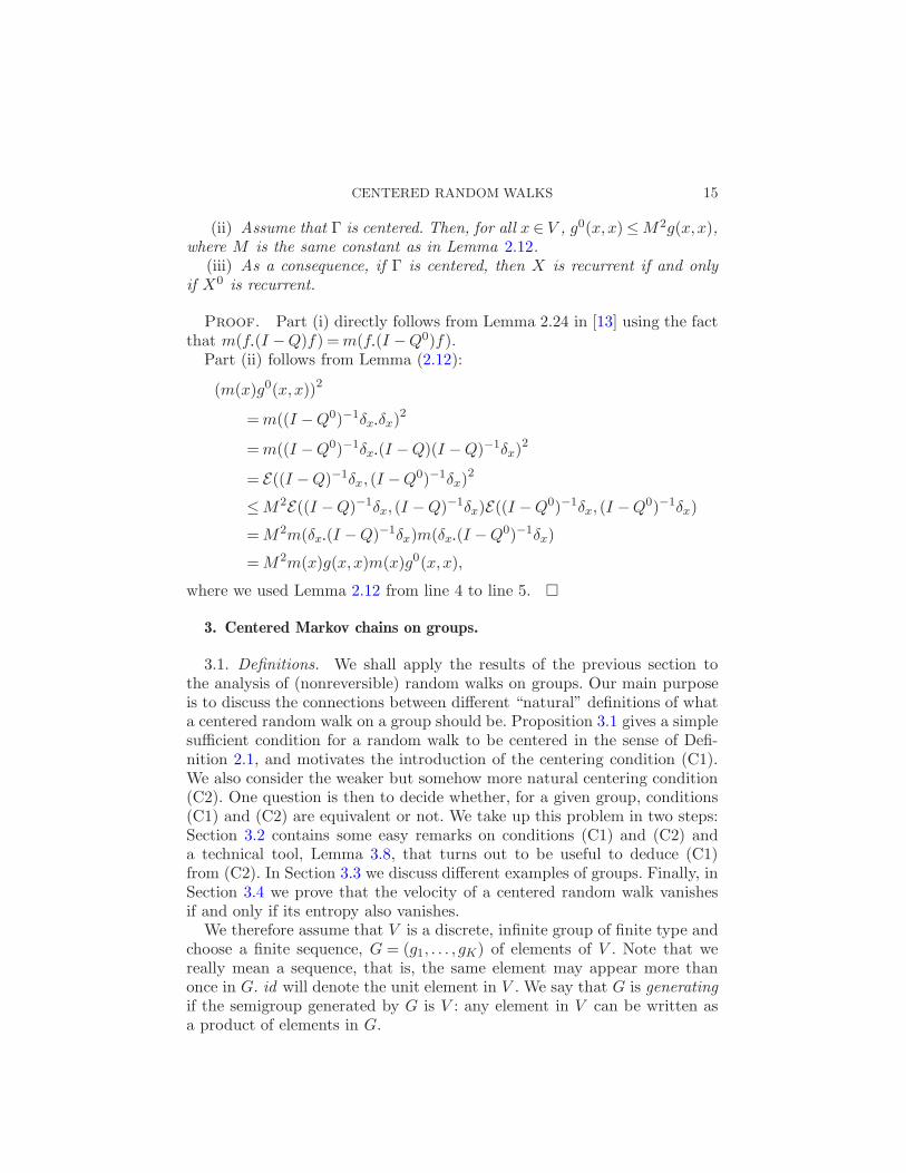
Proposition 2.13. (i) For any x∈ V , we have g(x,x) ≤ g0(x,x).

CENTERED RANDOM WALKS 15

(ii) Assume that Γ is centered. Then, for all x ∈ V , g0(x,x)≤ M2g(x,x),where M is the same constant as in Lemma 2.12.

(iii) As a consequence, if Γ is centered, then X is recurrent if and onlyif X0 is recurrent.

Proof. Part (i) directly follows from Lemma 2.24 in [13] using the factthat m(f

·(I −Q)f) = m(f

·(I −Q0)f).

Part (ii) follows from Lemma (2.12):

(m(x)g0(x,x))2

= m((I −Q0)−1δx·δx)2

= m((I −Q0)−1δx·(I −Q)(I −Q)−1δx)2

= E((I −Q)−1δx, (I −Q0)−1δx)2

≤ M2E((I −Q)−1δx, (I −Q)−1δx)E((I −Q0)−1δx, (I −Q0)−1δx)

= M2m(δx·(I −Q)−1δx)m(δx·

(I −Q0)−1δx)

= M2m(x)g(x,x)m(x)g0(x,x),

where we used Lemma 2.12 from line 4 to line 5. �

3. Centered Markov chains on groups.

3.1. Definitions. We shall apply the results of the previous section tothe analysis of (nonreversible) random walks on groups. Our main purposeis to discuss the connections between different “natural” definitions of whata centered random walk on a group should be. Proposition 3.1 gives a simplesufficient condition for a random walk to be centered in the sense of Defi-nition 2.1, and motivates the introduction of the centering condition (C1).We also consider the weaker but somehow more natural centering condition(C2). One question is then to decide whether, for a given group, conditions(C1) and (C2) are equivalent or not. We take up this problem in two steps:Section 3.2 contains some easy remarks on conditions (C1) and (C2) anda technical tool, Lemma 3.8, that turns out to be useful to deduce (C1)from (C2). In Section 3.3 we discuss different examples of groups. Finally, inSection 3.4 we prove that the velocity of a centered random walk vanishesif and only if its entropy also vanishes.

We therefore assume that V is a discrete, infinite group of finite type andchoose a finite sequence, G = (g1, . . . , gK) of elements of V . Note that wereally mean a sequence, that is, the same element may appear more thanonce in G. id will denote the unit element in V . We say that G is generatingif the semigroup generated by G is V : any element in V can be written asa product of elements in G.

16 P. MATHIEU

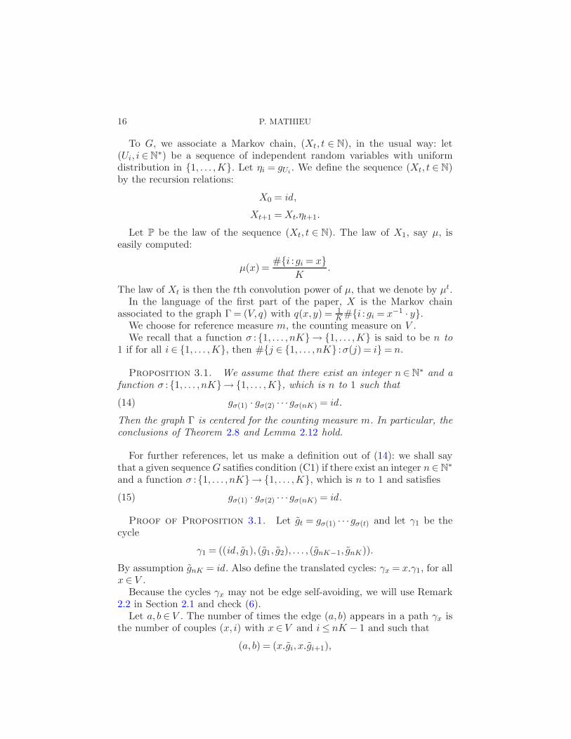
To G, we associate a Markov chain, (Xt, t ∈ N), in the usual way: let(Ui, i ∈ N

∗) be a sequence of independent random variables with uniformdistribution in {1, . . . ,K}. Let ηi = gUi

. We define the sequence (Xt, t ∈ N)by the recursion relations:

X0 = id ,

Xt+1 = Xt·ηt+1.

Let P be the law of the sequence (Xt, t ∈ N). The law of X1, say µ, iseasily computed:

µ(x) =#{i :gi = x}

K.

The law of Xt is then the tth convolution power of µ, that we denote by µt.In the language of the first part of the paper, X is the Markov chain

associated to the graph Γ = (V, q) with q(x, y) = 1K #{i :gi = x−1 · y}.

We choose for reference measure m, the counting measure on V .We recall that a function σ :{1, . . . , nK}→ {1, . . . ,K} is said to be n to

1 if for all i ∈ {1, . . . ,K}, then #{j ∈ {1, . . . , nK} :σ(j) = i} = n.

Proposition 3.1. We assume that there exist an integer n ∈ N∗ and a

function σ :{1, . . . , nK}→ {1, . . . ,K}, which is n to 1 such that

gσ(1) · gσ(2) · · ·gσ(nK) = id .(14)

Then the graph Γ is centered for the counting measure m. In particular, theconclusions of Theorem 2.8 and Lemma 2.12 hold.

For further references, let us make a definition out of (14): we shall saythat a given sequence G satifies condition (C1) if there exist an integer n ∈ N

∗

and a function σ :{1, . . . , nK}→ {1, . . . ,K}, which is n to 1 and satisfies

gσ(1) · gσ(2) · · ·gσ(nK) = id .(15)

Proof of Proposition 3.1. Let gt = gσ(1) · · ·gσ(t) and let γ1 be thecycle

γ1 = ((id , g1), (g1, g2), . . . , (gnK−1, gnK)).

By assumption gnK = id . Also define the translated cycles: γx = x·γ1, for all

x ∈ V .Because the cycles γx may not be edge self-avoiding, we will use Remark

2.2 in Section 2.1 and check (6).Let a, b ∈ V . The number of times the edge (a, b) appears in a path γx is

the number of couples (x, i) with x ∈ V and i ≤ nK − 1 and such that

(a, b) = (x·gi, x·

gi+1),

CENTERED RANDOM WALKS 17

or, equivalently,

a = x·gi and b = a

·gσ(i+1).(16)

If q(a, b) = 0, that is, a−1·

b /∈ G, then (16) has no solution. Otherwise, i beinggiven, x is uniquely determined by (16). Thus we are actually looking forthe number of i’s such that a−1

·b = gσ(i+1). This number is nKq(x, y), as

clearly follows from the definition of q and the assumption of σ being n to1. �

We now introduce a second centering condition: a given sequence satisfiescondition (C2) if for some integer n, (g1 · · ·gK)n ∈ [V,V ] or, equivalently,∑

i h(gi) = 0 for any homomorphism h from V to R; see Remark 3.6 below.Note that the condition (g1 · · ·gK)n ∈ [V,V ] is independent of the order in

which the product is computed. Indeed, changing the order in this productwould only multiply the result by an element in [V,V ].

Although condition (C1) is the one we needed to prove our results, con-dition (C2) is, to a certain extent, more natural. In particular, it is easier tocheck in examples.

It is also easy to see that (C1) implies (C2): indeed assume that (C1) holds.Then, since σ is n to 1, we obtain the product (g1 · · ·gK)n as a reordering ofthe elements of the product in (15). But changing the order in some productonly multiplies this product by an element in [V,V ]. Therefore (g1 · · ·gK)n ∈[V,V ] and (C2) holds.

Definition 3.2. We will say that the group V satisfies property (C) if,for any finite generating sequence, conditions (C1) and (C2) hold or fail si-multaneously. In extenso, V satisfies property (C) if, for any finite generatingsequence G = (g1, . . . , gK) such that for some n ∈ N

∗ we have (g1 · · ·gK)n ∈[V,V ], then there exist an integer n ∈ N

∗ and a function σ :{1, . . . , nK} →{1, . . . ,K}, which is n to 1 and satisfies

gσ(1) · gσ(2) · · ·gσ(nK) = id .(17)

Proposition 3.3.

(a) Nilpotent groups satisfy property (C).(b) The Baumslag–Solitar group BSq satisfies property (C).(c) The wreath product Z ≀Z satisfies property (C).(d) The free group F2 does not satisfy property (C).

Remark 3.4. From Proposition 3.3(a) and property (C) it follows thatif a generating set on a nilpotent group satisfies condition (C2), it thensatisfies the Carne–Varopoulos upper bound. As a matter of fact, it would

18 P. MATHIEU

also be possible to use Theorem 2.10 to get an upper bound of the formP[Xt = y|X0 = x]≤ Ct−r/2e−d2(x,y)/(Ct) for any centered random walk. (Herer is the volume growth exponent of the group.) But it should be pointedout that a more precise version of this last bound, and the correspondinglower bound, were obtained by Alexopoulos in [1] for more general centeredrandom walks than ours. Alexopoulos’ method is quite different from oursand does not use the equivalence between conditions (C1) and (C2).

3.2. Centering conditions. We start with some easy remarks on condi-tions (C1) and (C2):

Remark 3.5. The random walk X , associated to the finite sequence G,lives on the semigroup generated by G. If (C1) holds, it is easy to see thatthe semigroup generated by G is in fact a group.

Remark 3.6 (Homomorphisms on R). Let G = (g1, . . . , gK) be a finitesequence of elements of V .

First assume that for some n, (g1 · · ·gK)n ∈ [V,V ]. Then, for any homo-morphism h from V to R, we have

∑

i h(gi) = 0.Conversely, assume that, for any homomorphism from V to R, we have

∑

i h(gi) = 0. Then, for some n, (g1 · · ·gK)n ∈ [V,V ].Indeed, let γ be the image of the product g1 · · ·gK on V/[V,V ]. Either γ

has finite order—in which case the proof is finished—or it has infinite order.Since V/[V,V ] is Abelian, there exists a homomorphism h from V/[V,V ]to R such that h(γ) = 1. Then h induces a homomorphism on V such thath(g1 · · ·gK) = 1. This is in contradiction with the assumption that

∑

i h(gi) =0.

Thus we have proved that, for a given sequence G = (g1, . . . , gK), thefollowing two properties are equivalent:

(i) there exists n such that (g1 · · ·gK)n ∈ [V,V ],(ii) for any homomorphism h from V to R, we have

∑

i h(gi) = 0.

Remark 3.7. There are obvious counterexamples to the implication(C2) =⇒ (C1) for nongenerating sequences: choose K = 1. The condition(C1) is then equivalent to saying that g1 has finite order. Condition (C2)is satisfied if g1 ∈ [V,V ]. Thus if g1 ∈ [V,V ] but g1 is of infinite order, then(C2) is satisfied but (C1) is not. We avoid this situation by assuming thatthe set G generates V . Let us recall that the meaning of “generating” is: allelements of V belong to the semigroup generated by G, that is, any x ∈ Vcan be written as a product of elements in G.

The aim of the next section is to check that property (C) holds for somesimple enough groups. The proofs are based on the following combinatoriallemma:

CENTERED RANDOM WALKS 19

Lemma 3.8. Choose a finitely generated group, V , and some elementa ∈ V . The following two properties are equivalent:

(i) For any finite generating sequence, G = (g1, . . . , gK), such that(g1 · · ·gK)n ∈ [V,V ] for some n ∈ N

∗, then (C1) holds.(ii) For any finite generating sequence, G = (g1, . . . , gK), such that

(g1 · · ·gK)n ∈ [V,V ] for some n ∈ N∗, then (C1) holds for the enlarged se-

quence (g1, . . . , gK , a, a−1).

Proof. Of course (i) implies (ii). Assume that (ii) is verified. Let Gbe some finite generating sequence such that (g1 · · ·gK)n ∈ [V,V ]. We checkthat G satisfies (C1).

Since G generates V , we can write

a = gσ1(1) · · ·gσ1(k1) and a−1 = gσ2(1) · · ·gσ2(k2),

for some applications σ1 :{1, . . . , k1}→ {1, . . . ,K} and σ2 :{1, . . . , k2}→ {1,. . . ,K}. Call G1 the sequence of elements in V obtained by forming all theproducts of elements of G of length k1. In other words,

G1 = (gσ1(1) · · ·gσ1(k1);σ1 ∈ {1, . . . ,K}{1,...,k1}).

(Remember G1 is a sequence, not a set. The same element may appear morethan once.) Similarly, define G2 to be the sequence of elements in V obtainedby forming all the products of elements of G of length k2:

G2 = (gσ2(1) · · ·gσ2(k2);σ2 ∈ {1, . . . ,K}{1,...,k2}).

Thus a ∈ G1 and a−1 ∈ G2. Finally let G be the concatenation of the se-quences G, G1 and G2. Then G has K = K + Kk1 + Kk2 elements.

We claim that G satisfies the requirements of (ii). Indeed G generates Vsince it contains G and G generates V . We also have a, a−1 ∈ G. If we formthe nth power of the product of the elements of G, we get

(g1 · · · gK)n = ((g1 · · ·gK)Πσ1(gσ1(1) · · ·gσ1(k1))Πσ2(gσ2(1) · · ·gσ2(k2)))n

= (g1 · · ·gK)n(1+k1Kk1−1+k2Kk2−1) mod([V,V ]),

where the second equality holds up to reordering.Since, by assumption, (g1 · · ·gK)n ∈ [V,V ], we see that (g1 · · · g2)

n ∈ [V,V ].Therefore we deduce that G satisfies the condition (C1): there exist somenumber n and an application σ :{1, . . . , nK}→ {1, . . . , K} such that

gσ(1) · · · gσ(nK) = id ,(18)

and σ is n to 1. Imagine you rewrite the product (18) with the elements ofG. From the construction of G, it then follows that each element of G willappear exactly n(1+Kk1−1 +Kk2−1) times. We have thus checked condition(C1) for the generating sequence G.

Note that all over this proof the roles of the different elements of G aresymmetric. �

20 P. MATHIEU

3.3. Examples and proof of Proposition 3.3. As a preliminary, let us firstconsider the simplest example:

Example 3.9 (Periodic groups). We assume that all elements of V havefinite order. Thus V is a periodic group, also called a torsion group. Givenany finite set G, we can choose n such that gn

i = id for all i ∈ {1, . . . ,K}.We then define σ(i) to be the integer part of 1 + i−1

n . σ is clearly n to 1.Besides,

gσ(1) · · ·gσ(nK) = gn1 · · ·gn

K = id .

As a conclusion the graph Γ associated to G is centered.We shall now extend this result to more general random walks on V : let

µ be a probability measure on V with finite support. Consider the Markovchain with transition rates q(x, y) = µ(x−1

·y). For x ∈ V and g in the support

of µ, define the cycle γx,g = (x,x·g,x

·g2, . . . , x

·gp(g)), where p(g) is the order

of g. Let qg = 1p(g)µ(g).

Choose a, b ∈ V . For fixed g, count the total number of occurrences of theedge (a, b) in cycles of the form γx,g, where x ranges through V . We get:p(g) if a−1

·b = g and 0 otherwise. Therefore∑

x,g

qgN((a, b), γx,g) =∑

g

µ(g)1a−1·

b=g = µ(a−1·

b) = q(a, b).

We have checked condition (6) and therefore the graph Γ = (V, q) is centeredfor the counting measure.

Example 3.10 (Abelian case). Assume that the product g1 · · ·gK hasfinite order, say p. Then it is easy to construct a function σ, which is p to1 and satisfies (15). Now assume that V is Abelian. If (C1) holds, then wemust have (g1 · · ·gK)n = 1. [This is just a reordering of the product in (15).]Then g1 · · ·gK has finite order. Thus we see that, for an Abelian group, (C1)is fullfilled if and only if the product g1 · · ·gK has finite order. In particular,Abelian groups satisfy property (C).

Proof of Proposition 3.3. (a) Nilpotent groups satisfy property (C).We proceed by induction on the nilpotency class of V . Let V = V0 > V1 >· · ·> Vr = {id} be the lower central series of V with Vi+1 = [V,Vi]. Let Z bethe center of V . The case r = 1 corresponds to an Abelian group V and wasalready discussed in Example 3.10.

Note that Vr−1 is Abelian and finitely generated. We may, and do, chooseelements (xi, yi, i = 1, . . . , k) such that the set ([xi, yi], i = 1, . . . , k) generatesVr−1. Finally notice that Vr−1 ⊂ Z. Therefore if x, y ∈ V are such that [x, y] ∈Vr−1, then [xα, yβ] = [x, y]αβ for all nonnegative α and β.

CENTERED RANDOM WALKS 21

Assume now that the statement of the proposition is true for any nilpotentgroup of class r− 1 or less. Let V be of class r. Let G = (g1, . . . , gK) be a fi-nite generating sequence and let n be such that (g1 · · ·gK)n ∈ [V,V ]. We wishto prove that condition (C1) holds. Using Lemma 3.8, it is sufficient to provethat the sequence (g1, . . . , gK , x1, . . . , xk, y1, . . . , yk, x

−11 , . . . , x−1

k , y−11 , . . . , y−1

k )satisfies (C1).

We use the induction assumption: the group V/Vr−1 is nilpotent of classstrictly less than r. Therefore there is an integer p and a 1 to p functionσ :{1, . . . , pK}→ {1, . . . ,K} such that gσ(1) · · ·gσ(pK) ∈ Vr−1. Therefore thereexist l ≥ 0, l ≤ k and α1, . . . , αl ∈ Z such that gσ(1) · · ·gσ(pK)[x1, y1]

α1 · · ·[xl, yl]

αl = id . Interchanging the roles of xi and yi when necessary, we mayassume that the αi’s are nonnegative.

Let α be the product α = α1 · · ·αl. Note that [xi, yi]αiα = [xαi

i , yαi

i ]α/αi .We have

id = (gσ(1) · · ·gσ(pK)[x1, y1]α1 · · · [xl, yl]

αl)α

= (gσ(1) · · ·gσ(pK))α[x1, y1]

α1α · · · [xl, yl]αlα

(because [xi, yi] ∈ Vr−1 ⊂Z)

= (gσ(1) · · ·gσ(pK))α[xα1

1 , yα11 ]α/α1 · · · [xαl

l , yαl

l ]α/αl

= (gσ(1) · · ·gσ(pK))α[xα1

1 , yα11 ]α/α1 · · · [xαl

l , yαl

l ]α/αl(x1x−11 y1y

−11 )α(p−1)

× · · · × (xlx−1l yly

−1l )α(p−1)(xl+1x

−1l+1yl+1y

−1l+1)

αp · · · (xkx−1k yky

−1k )αp.

In this last expression, each gi appears αp times; each term of the formxi, x−1

i , yi or y−1i with i ≤ l appears α + α(p − 1) = αp times; each term

of the form xi, x−1i , yi or y−1

i with i > l appears αp times. Thus we havechecked condition (C1).

(b) The Baumslag–Solitar group BSq satisfies property (C). By definition,the Baumslag–Solitar group BSq is the group with presentation 〈a, b|ab =bqa〉, where q ≥ 2 is an integer. It is an example of an amenable, solvablegroup of exponential volume growth. It is also the subgroup of the affinegroup of R generated by the transformations x → x + 1 and x → qx.

From the presentation, it is obvious that any homomorphism of V on R

should vanish on b. It is possible to prove that elements on V can be writtenin the form x = (a−lbmal)ak. In particular, if x ∈ [V,V ], then x must be ofthe form x = a−lbmal for some l ≥ 0 and m ∈ Z. We shall use the relation[bβ , aα] = bβ(1−qα).

Let G = (g1, . . . , gK) be a finite generating sequence and choose n suchthat (g1 · · ·gK)n ∈ [V,V ]. We wish to prove that condition (C1) holds. Ac-cording to Lemma 3.8, it is sufficient to prove (C1) for the enlarged sequence(g1, . . . , gK , a, a−1, b, b−1). Let l ≥ 0 and m ∈ Z be such that (g1 · · ·gK)n =a−lbmal.

22 P. MATHIEU

First assume that m ≥ 0. Choose α such that qα − 1 ≥ m and choose jsuch that j(qα − 1) ≥ α + l. Let k = j(qα − 1), β = mj, k1 = nk − α − l ≥ 0and k3 = nk − β ≥ 0.

We have

(g1 · · ·gK)kna−l[bβ , aα]alak1a−k1bk3b−k3

= (a−lbmal)ka−lbβ(1−qα)al = a−lbkmbβ(1−qα)al = id ,

since km + β(1− qα) = 0.Considering the expression (g1 · · ·gK)kna−l[bβ , aα]alak1a−k1bk3b−k3 as a

word in the alphabet G, we see that: the elements gi, i ≤ K, appear eachexactly kn times; a and a−1 appear α+ l + k1 = kn times; b and b−1 appearβ + k3 = kn times. Therefore we have checked (15).

The proof is done very much the same way if m ≤ 0.(c) The wreath product Z ≀ Z satisfies property (C). Z ≀ Z is isomorphic

to the group of affine transformations of R generated by the translationx → x + 1 and the homothety x → ax where a is transcendental. It is alsoa semidirect product of Z and a direct product of countably many copies ofZ. It is therefore a two-step solvable group of finite type, although it is notfinitely presented.

To be more precise, and quoting from [13]: a configuration η is a functionfrom Z to Z such that the set {x :η(x) 6= 0} is finite. Equipped with pointwiseaddition, the set of configurations is a group, say Z. Z acts on Z by automor-phisms via (y, η) → Tyη where Tyη(x) = η(x − y). The resulting semidirectproduct is the wreath product Z ≀Z. We denote by ε the natural projection ofZ ≀Z onto Z and by H the projection of Z ≀Z on Z. Thus any element of Z ≀Z isa couple a = (ε(a), η) where η ∈ Z. Z ≀Z is generated by the following four ele-ments: τ1 = (1,0), τ−1 = τ−1

1 = (−1,0) and σ1 = (0, η1), σ−1 = σ−11 = (0, η−1),

where η1(0) = 1, η1(x) = 0 if x 6= 0, η−1(0) = −1, η−1(x) = 0 if x 6= 0. We willuse |a| to denote the distance between a ∈ Z ≀Z and id in the metric inducedby the generating set {τ1, τ−1, σ1, σ−1}.

ε is a homomorphism of Z ≀ Z on R. Another such homomorphism isa→

∑

x∈Z H(a)(x).Let G be a finite generating set: G = {g1, . . . , gK}. Assume that G satisfies

condition (C2). Therefore∑K

i=1 ε(gi) = 0 and∑K

i=1

∑

x∈Z H(gi)(x) = 0.Using Lemma 3.8, in order to prove that condition (C1) holds we may, and

will, replace G by the enlarged generating set: G′ = {τ1, τ1, τ−1, τ−1, σ1, σ−1, g1,. . . , gK}.

We let φ be the product φ = g1 · · ·gK and φn = φ(τ1·φ)n. In the sequel to

this proof, C and M will denote some constants that depend on G but noton n.

We first note that ε(φn) = n, since ε(φ) = 0. Also note that H(φn)(x) =∑n

j=0 H(φ)(x − j) =∑x

j=x−n H(φ)(j). And since∑

x∈Z H(φ)(x) = 0, then

CENTERED RANDOM WALKS 23

there must be a constant M such that H(φn)(x) 6= 0 implies that x ∈[−M,M ] or x ∈ [n − M,n + M ]. Thus φn is of the form φn = A(n)τn

1 B(n)

for some elements A(n) and B(n) such that |A(n)|+ |B(n)| ≤ C, for some con-stant C (that does not depend on n!). Which means that we can write bothA(n) and B(n) as products of elements of {τ1, τ−1, σ1, σ−1} with less than Csymbols.

Thus we have obtained a trivial product: id = φn(B(n))−1τn−1(A

(n))−1 inwhich:

(i) each element gi appears n + 1 times;(ii) the numbers of occurrences of σ1 and σ−1 are equal because

∑

x∈Z H(φn)(x) = 0 =∑

x∈Z H(A(n)B(n))(x). Call this number b(n). b(n) is

bounded by some constant that does not depend on n, since |A(n)|+ |B(n)| ≤C;

(iii) by the same argument, τ1 and τ−1 appear the same number of times,say a(n) and a(n) ≤ n + C.

Choose n such that b(n) ≤ n and a(n) ≤ 2n + 2. We obviously have id =

φnB(n)−1τn−1A

(n)−1(τ1τ−1)2n+2−a(n)

(σ1σ−1)n+1−b(n)

and this last expressionproves (15).

(d) The free group F2 does not satisfy property (C). Choose G = (g1 =a, g2 = a−1, g3 = b, g4 = b−1, g5 = b−2, g6 = ababa−2). Clearly, G generates.Besides

g1g6g3g5g2g4 = a2·bab

·a−2

·b−1a−1b−1 = [a2, bab] ∈ [V,V ].

Let n be a positive integer. Let γ be an element of V that can be writtenas a product of elements in G using exactly n times each of the gi’s. Let usprove that γ 6= id .

First write γ as a product of elements in G with n occurrences of eachgi. We label the different occurrences of g6 by the numbers 1 to n accordingto the order in which they appear. Replace the gi’s by their expressionsin terms of a, b, a−1, b−1. We obtain a nonreduced word in the alphabet(a, b, a−1, b−1). The letters coming from the ith occurrence of g6 are labeledi. We run the following algorithm to reduce it step by step: read the wordstarting from the left; do all cancellations you find on your way; start againwhen you reach the end of the word. For i, j ∈ {1, . . . , n}, we draw an edgebetween i and j if, while running the cancellation algorithm, one of the “a−1”with label i cancels with one of the “a” with label j or one of the “a−1”with label j cancels with one of the “a” with label i. This way we obtain anonoriented graph structure on {1, . . . , n}. Let J be the total number of edgesof this graph. If J < n, then γ is not id . Indeed, there are 3n occurrences of“a−1” in the nonreduced word, n of them coming from g2 and 2n of themcoming from g6. Of the 2n occurrences of “a−1” coming from g6, J cancel

24 P. MATHIEU

with some “a” coming from some occurrence of g6, and, at most n of themcancel with an “a” coming from g1. Thus, after the algorithm has run, therewill be at least (2n− (n + J)) “a−1” left in the reduced word.

The graph structure we have built on {1, . . . , n} satisfies the followingproperties:

(i) it has no double edge, that is, we did not draw two edges from i toj. This is due to the presence of the “b” between the two “a” in g6;

(ii) it has no loop of the form i ↔ j ↔ i;(iii) a configuration of the form i1 ↔ i2, i3 ↔ i4 with i4 strictly between

i1 and i2 implies that i3 lies between i1 and i2 (in the broad sense).

(iii) follows from the definition of the algorithm.Thus the graph contains no cycle. Indeed, if i1 ↔ i2 ↔ · · · ↔ ik was a

minimal cycle (ik = i1 and the labels i1, . . . , ik−1 are pairwise different),then, from (iii), we deduce that, up to a circular permutation or runningthe cycle in the opposite order, the sequence i1, . . . , ik−1 must be increasing.But this is impossible because the “b” would not cancel.

We conclude that the graph has no cycle. Therefore its number of edgesis strictly less than n. �

3.4. On the velocity. Given the finite generating set G, we consider theinduced distance on V : d(x, y) is the minimum number of elements in G ∪G−1 whose product equals x−1y. This definition corresponds to the definitionof distance we used in Section 2.1.

The speed of the random walk (Xt, t ∈ N) is L = limt→∞1t d(id ,Xt). The

entropy of the random walk is h = limt→∞−1t logµt(Xt) where µ is the law

of X1 (and therefore µt is the law of Xt). The subadditive ergodic theoremimplies that the limits defining L and h exist in the almost sure sense aswell as in the L1 sense; both L and h are nonnegative numbers. (See [13],Theorem (8.14), [5], Section IV or [9], Theorem 1.6.4.)

It is known, without any symmetry assumption, that h = 0 if and only ifthe Poisson boundary of the random walk is trivial; see [5], Section IV or[9], Section 1.6. From Corollary 1 in [12] it follows that h = 0 if L = 0. Theconverse follows from the classical Carne–Varopoulos inequality in the caseof symmetric random walks. We extend this result in the centered case inthe next proposition and then show in an example how this can be used toprove that some random walks have vanishing speed.

Proposition 3.11. Assume that (C1) holds. If the entropy vanishes,then L = 0.

Proof. It is straightforward once we recall the Carne–Varopoulos boundfrom Theorem (2.8): for some constant C, we have

µt(x) ≤Ce−d2(id ,x)/(Ct).

CENTERED RANDOM WALKS 25

For any α > 0, we then have

0 = h = lim−1

tE[logµt(Xt)] = lim−

1

t

∑

x∈V

logµt(x)µt(x)

≥ lim−1

t

∑

x;d(id ,x)≥αt

log µt(x)µt(x)

≥ lim1

t

∑

x;d(id ,x)≥αt

(

− logC +d2(id , x)

Ct

)

µt(x)

≥α2

Clim

∑

x;d(id ,x)≥αt

µt(x) =α2

CP[Xt ≥ αt].

Therefore P[Xt ≥ αt]→ 0 for any α > 0 and thus L = 0. �

Example 3.12. We discuss the application of the last proposition in thecase of Z ≀Z using the same notation as in the proof of Proposition (3.3)(c).

Let G be a finite generating sequence in Z ≀ Z satisfying condition (C1)or equivalently condition (C2). Since G generates Z ≀ Z, its image by thehomomorphism ε generates Z. Therefore the random walk ε(Xt) is recurrent.It then follows from the fact that Z ≀Z is a semidirect product of a recurrentgroup and an Abelian group that the Poisson boundary is trivial (see [8],Theorem 3.1), and therefore h = 0 and therefore, applying our proposition,L = 0.

It should be noted that if we drop the assumption that G generates, thesituation becomes quite different. Choose, for instance, G = {g1 = (+2, T1σ1),g2 = (−2, σ−1)}. Then G satisfies condition (C2) since ε(g1) + ε(g2) = +2−2 = 0 and

∑

x H(g1)(x)+H(g2)(x) =∑

x σ1(x)+σ−1(x) = 0. Clearly, G doesnot satisfy condition (C1). As a matter of fact, there is no way to write idas a nonempty product of g1 and g2. Besides L 6= 0. Indeed, each multipli-cation by g1 adds a “1” at an odd location in Z and each multiplication byg2 adds a “−1” at an even location in Z. Thus

∑

x∈Z H(Xt)(2x) = −#{s≤

t :X−1s−1Xs = g1} and similarly

∑

x∈Z H(Xt)(2x + 1) = #{s ≤ t :X−1s−1Xs =

g2}. So∑

x∈Z H(Xt)(2x + 1)−H(Xt)(2x) = t and L > 0.

Acknowledgments. Many thanks to Christophe Pittet and Laurent Saloff-Coste for their help, suggestions and interest in this work. I also thank thereferees for their comments.

REFERENCES

[1] Alexopoulos, G. K. (2002). Random walks on discrete groups of polynomial volumegrowth. Ann. Probab. 30 723–801. MR1905856

26 P. MATHIEU

[2] Baldi, P., Lohoue, N. and Peyriere, J. (1977). Sur la classification des groupesrecurrents. C. R. Acad. Sci. Paris Ser. A–B 285 1103–1104. MR0518008

[3] Carne, T. K. (1985). A transmutation formula for Markov chains. Bull. Sci. Math.

109 399–405. MR0837740[4] Chen, M. F. (1991). Comparison theorems for Green functions of Markov chains.

Chinese Ann. Math. Ser. A 12 237–242. MR1130250[5] Derriennic, Y. (1980). Quelques applications du theoreme ergodique sous-additif.

Asterisque 74 183–201. MR0588163[6] Hebisch, W. and Saloff-Coste, L. (1993). Gaussian estimates for Markov chains

and random walks on groups. Ann. Probab. 21 673–709. MR1217561[7] Jiang, D. Q., Qian, M. and Qian, M. P. (2004). Mathematical Theory of Nonequi-

librium Steady States. On the Frontier of Probability and Dynamical Systems.

Lecture Notes in Math. 1833. Springer, Berlin. MR2034774[8] Kaimanovich, V. A. (1991). Poisson boundaries of random walks on discrete solvable

groups. In Probability Measures on Groups X (H. Heyer, ed.) 205–238. Plenum,New York. MR1178986

[9] Kaimanovich, V. A. (2001). Poisson boundary of discrete groups. Available atname.math.univ-rennes1.fr/vadim.kaimanovich/.

[10] Kalpazidou, S. L. (1995). Cycle Representations of Markov Processes. Springer,New York. MR1336140

[11] Varopoulos, N. Th. (1985). Long range estimates for Markov chains. Bull. Sci.

Math. 109 225–252. MR0822826[12] Vershik, A. M. (2000). Dynamic theory of growth in groups: Entropy, boundaries,

examples. Russ. Math. Surveys 55 667–733. MR1786730[13] Woess, W. (2000). Random Walks on Infinite Graphs and Groups. Cambridge Univ.

Press. MR1743100

CMI

39 rue Joliot-Curie

13013 Marseille

France

E-mail: pierre.mathieu@cmi.univ-mrs.fr