New Considerations on Analytical Solutions Employed in Tracer Flow Modeling

Transport in Porous Media 54: 221–237, 2004.c© 2004 Kluwer Academic Publishers. Printed in the Netherlands. 221

New Considerations on Analytical SolutionsEmployed in Tracer Flow Modeling

MANUEL CORONADO1,∗, JETZABETH RAMIREZ1 and FERNANDOSAMANIEGO2

1Instituto Mexicano del Petroleo, Eje Central Lazaro Cardenas 152, 07730 Mexico D.F., Mexico2Facultad de Ingenierıa, Universidad Nacional Autonoma de Mexico, Ciudad Universitaria, 04510Mexico D.F., Mexico

(Received: 14 May 2002; in final form: 12 May 2003)

Abstract. A methodology commonly used to obtain analytical and semi-analytical solutions todescribe spike and finite-step tracer injection tests is discussed. In these cases, solutions to thediffusion–convection equation are derived from the solution of a different problem, namely the con-tinuous injection of a tracer. Within this procedure, spike injection results from the time derivativeof this solution, and finite-step injection from the superposition of two solutions shifted in time.In this paper we show that although this methodology is mathematically correct, attention shouldbe paid to the properties of the solutions. Their boundary conditions may not represent physicallyacceptable situations, since these conditions are inherited from a different problem. The applicationof the methodology to a simple one-dimensional case of a tracer pulse diffusing in a homogeneous,semi-infinite reservoir shows serious problems regarding boundary conditions and mass conserva-tion. These problems has not probably been found before since tracer breakthrough curves are notvery sensitive to them. However, the problems clearly show up when the tracer distribution in spaceis analyzed. We conclude that the traditional methodology should not be employed. Equations shouldbe solved imposing the specific boundary and initial conditions corresponding to the original systemunder consideration.

Key words: tracer, diffusion, dispersion, transport, flow, modeling, porous media, boundaryconditions.

Nomenclature

a constant (T(= time)).aFS constant (TM/L3).a0 constant (TM/L3).a1 constant (TM/L3).A effective cross-section perpendicular to the flow direction

(L2(= [length]2)).A1, A2 constants (dimensionless).b constant (dimensionless).C(x, t) tracer concentration (M/L3).C(x, s) tracer concentration in Laplace space (MT/L3).

∗Author for correspondence: e-mail: [email protected]

222 MANUEL CORONADO ET AL.

Cc(x, t) tracer concentration of continuous injection (M/L3).Cc(x, s) tracer concentration of continuous injection in Laplace space (MT/L3).Cg(x, t) true spike tracer concentration obtained from a Dirac delta (M/L3).Cg(x, s) Laplace tracer concentration of a true pulse (MT/L3).CFS(x, t) tracer concentration of finite-step injection (M/L3).CS(x, t) tracer concentration obtained from the time derivative (M/L3).C0 constant tracer concentration (M/L3).C1(x, t), C2(x, t) two solutions of Equation (1) (M/L3).D dispersion coefficient (L2/T).f (x) arbitrary function of x (M/L2T).J mass flow as a vector (M/L2T).Jx mass flow in x-direction (M/L2T).mJ total cumulative mass through a cross-section A (M).m0 total mass injected per unit area A in the half space (0,∞) (M).MI total mass injected per unit area A in the full space (−∞, ∞)

(M(= mass)).n variable (L−1).s Laplace conjugate variable of time (T−1).t time (T).�t tracer injection period (T).t1, t2, t3 constant times: t1 < t2 < t3 (T).u velocity of a frame of reference (L/T).v constant average flow velocity in x-direction (L/T).v constant average flow velocity (a vector) (L/T).x space variable (L).x′ space variable in a moving reference frame (L).x1, x2, x3 constant positions in space: x1 < x2 < x3 (L).

Greek Lettersξ variable (dimensionless).τ1, τ2 constants (T).

SymbolsL, L−1 Laplace transform and inverse Laplace transform.O(z) terms of order of magnitude of (z).δ(x) Dirac delta function (L−1).

1. Introduction

Tracers have long been used by petroleum and water reservoir engineers to obtaininformation on reservoir structure. To perform inter-well tests, tracers are injectedinto the reservoir at a selected well, and its breakthrough at different productionwells is observed. Through these tests the preferential flow channels inside thereservoir can be determined. Further, an analytical model that appropriately matchthe field results, that is, tracer concentration as function of time at the productionwell, could additionally provide useful information regarding average reservoirproperties such as convection velocity, diffusion coefficient, reservoir porosity,

TRACER FLOW MODELING 223

fracture width, block size, etc. Thus, the set up of adequate mathematical mod-els is of practical importance. In the past years different analytical models havebeen developed to describe tracer behavior in homogeneous and fractured reser-voirs, see, for example, Coats (1963), Bear (1972), Tang et al. (1981), Walkupand Horne (1985), Ramırez et al. (1990, 1995), Abbaszadeh (1995) and Kass(1998). A mathematical tool employed in some of these models (Abbaszadeh,1995; Ramırez et al., 1995; Walkup and Horne, 1985) to obtain expressions thatdescribe spike and finite-step tracer injection tests, uses the tracer concentrationcorresponding to continuous injection, say Cc(x, t). Spike injection is obtainedfrom the time derivative ∂Cc(x, t)/∂t , and the finite-step injection from the super-position [Cc(x, t)−Cc(x, t −�t)], where �t is the injection time period. The firstprocedure is particularly useful when Laplace transform in time is employed tosolve the equations, since time derivative in Laplace space is just a multiplicationby the conjugate variable.

The purpose of this paper is to show that solutions obtained by this methodmight result physically incorrect since the associated boundary conditions are in-appropriate. The analysis of the tracer space distribution results very illustrativeto see it. The paper is organized as follows. In Section 2 the cited methodologyis presented. Some basic conditions that solutions should satisfy are discussed inSection 3. In Section 4 the solutions for some cases of interest are obtained andthe problems appearing by using this methodology are analyzed. Conclusions aregiven in Section 5.

2. Solutions of the Convection–Diffusion Equation

Let us consider the case of a linear and homogenous partial differential trans-port equation with constant coefficients, specifically the equation that describesdiffusion and convection of a tracer in a one-dimensional, homogenous reservoir,

∂C

∂t− D

∂2C

∂x2+ v

∂C

∂x= 0, (1)

where C is the tracer concentration as function of x and t , D is a constant diffusioncoefficient, and v a constant average flow velocity. Equation (1) together with a fullset of boundary and initial conditions determine the solution C(x, t) completely.

If C(x, t) is a solution of Equation (1), then ∂C(x, t)/∂t is also a solution ofthis equation. To prove it, we can evaluate [∂/∂t −D∂2/∂x2 +v∂/∂x](∂C/∂t) andobtain (∂/∂t)[∂C/∂t − D∂2C/∂x2 + v∂C/∂x] after interchange of the time andspace derivatives. This expression equals zero thanks to Equation (1), what provesthe statement. By the same procedure, it can be shown that derivatives of C(x, t) atany order in t and x is also a solution. It is important to be noticed that the boundaryand initial conditions satisfied by these new solutions are not free, they are alreadyfixed by the original problem (except for a multiplying constant).

Further, if C1(x, t) and C2(x, t) are solutions of Equation (1), then any linearcombination of them, say A1C1(x, t + τ1) + A2C2(x, t + τ2) with A1, A2, τ1 and


τ2 constants, is also a solution (superposition principle). As in the previous case,the boundary and initial conditions of the new solution are already fixed by theconditions satisfied by C1 and C2.

The knowledge of the properties of these new solutions above mentioned is ofgreat relevance, in particular when our interest is set on adequate models for fittingfield data to determine reservoir properties.

In this paper we will analyze solutions of the form found in the reservoir tracertest literature, for spike injection

CS(x, t) = a∂Cc

∂t, (2)

and for finite-step injection

CFS(x, t) = b[Cc(x, t) − Cc(x, t − �t)], (3)

where Cc(x, t) is a solution for the continuous injection case, a and b are constantsand �t is the injection period of time. If we take b proportional to 1/�t then CFS

in Equation (3) goes into CS in the limiting case �t → 0. Thus, the finite-stepinjection model in Equation (3) is a generalization of the spike injection model inEquation (2).

3. Some Basic Conditions

A fundamental requirement in any solution of a transport equation without sourcesor losses, as the case of Equation (1), is that the total mass of the tracer injected ina reservoir is conserved. The conservation of the mass is inherent to Equation (1),since it results from the conservation law ∂C/∂t + ∇ · J = 0 together with J =−D∇C+vC, C = C(x, t) and v in the x-direction. Therefore, the total tracer massin the reservoir, after its injection is completed and when no loss mechanisms arepresent (like rock adsorption or radioactive decay), should keep constant. It means

A

∫ +∞

−∞C(x, t) dx = MI, (4)

where C(x, t) is any solution of Equation (1), in particular those solutions obtainedby the methods mentioned in the previous section, MI is the total tracer massinjected, and A is a cross-section perpendicular to the flow direction. In a porousmedium, A is an effective cross-section that includes rock porosity.

In some of the tracer transport problems considered in the literature the regionof interest is not the whole space, but 0 � x � ∞. In this case and after the tracerinjection is fully completed, a mass conservation condition can be set as

A

∫ ∞

0C(x, t) dx = m0, (5)


where m0 is a constant equal to the total mass of tracer in the region of analysis.When x-symmetry is imposed, m0 = MI/2 follows, however not always this sym-metry is present. Equation (5) is a condition that determines the constants a or b

involved in expressions (2) or (3) in terms of m0.It should be observed that solutions describing continuous injection involve a

constant, C0, which is the tracer concentration at the injection site. Solutions CS

and CFS in Equations (2) and (3) will therefore contain that constant C0 since theyare derived from that expression. However, C0 in the new solutions CS and CFS

plays the role of a constant without a prefixed physical meaning. In reality, C0

would become part of the constants a or b in Equations (2) or (3). In well-definedsolutions CS and CFS, the constants a and b have a physical meaning linked to thetotal mass injected in the reservoir.

Another important quantity to be considered in the analysis of mass conser-vation is the total cumulative tracer mass, mJ , flowing in x-direction through aneffective cross-section A, perpendicular to the flow direction, at a given position x.This means

mJ = A

∫ ∞

0Jx(x, t) dt, (6)

where Jx(x, t) is the x-component of the tracer flow (mass per unit area per unittime). In the case involved in our treatment, Equation (1), it holds

Jx = −D∂C

∂x+ vC, (7)

where C = C(x, t) is any tracer concentration, in particular it may be CS(x, t)

or CFS(x, t). Notice that the time integral involved in mJ is from 0 to ∞, and thecumulative flow should therefore become equal to the total tracer mass present inthe reservoir.

Substitution of Equation (7) in Equation (6) yields

mJ

A= −D

∂

∂x

∫ ∞

0C(x, t) dt + v

∫ ∞

0C(x, t) dt. (8)

Notice that this expression contains an integral of C(x, t) in time, while m0 inEquation (5) involves an integral of C(x, t) in space.

There are several simplified mathematical procedures that may help in the eval-uation of the integrals in m0 and mJ . These procedures are shown in Appendix A,and will be used along the paper.

4. Discussion of the Problems Appearing in the Solutions

Although the problems we are going to analyze here also appear when convection isinvolved, in what follows we are going to restrict ourselves to the case of diffusionwithout convection in order to simplify and clarify the misleadings found in the


analytical solutions obtained by the methods mentioned in Section 2. At the end ofthis section, however, a brief discussion of the results with convection is presented.

We therefore treat Equation (1) with v = 0:

∂C

∂t− D

∂2C

∂x2= 0, (9)

and analyze its solutions from different perspectives.

4.1. AN INITIAL DIRAC DELTA PULSE

In order to have a reference to compare the solution CS with, we will first treatthe case of a genuine or true pulse, this means a pulse that at the initial time is aDirac delta. The initial and boundary conditions to be used are Cg(x, t = 0) =(MI/A)δ(x), where MI/A is the total mass injected per unit element of cross-section, and Cg(|x| → ∞, t) = 0. The solution to this problem is well known,see, for example, Crank (1956); it is

Cg(x, t) = MI/A√4πDt

e−x2/4Dt . (10)

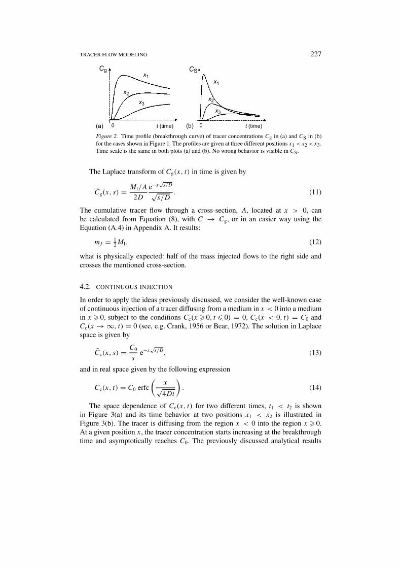
The behavior of Cg as function of x can be seen in Figure 1(a) for three differenttimes, t1 < t2 < t3. It is to be noticed that the pulse decreases and spreads withtime, keeping its maximum at x = 0. Due to mass conservation the total areabelow the curve in the region (−∞, ∞) keeps constant, and since Cg is symmetric,also the area below the curve in the region (0, ∞) keeps constant. In Figure 2(a)the behavior of Cg observed as a function of time at three different distancesfrom the injection site, x1 < x2 < x3 is illustrated. After a breakthrough timeperiod, the tracer concentration grows rapidly, reaches a maximum and decreasesslowly in time.

Figure 1. Space distribution of the tracer concentrations of a pulse diffusing without convec-tion, (a) in the case of a true Dirac pulse, Cg, and (b) in the case of a spike obtained froma time derivative, CS. The concentration is shown at three different times t1 < t2 < t3. Aphysically incorrect behavior is apparent in CS.


Figure 2. Time profile (breakthrough curve) of tracer concentrations Cg in (a) and CS in (b)for the cases shown in Figure 1. The profiles are given at three different positions x1 < x2 < x3.Time scale is the same in both plots (a) and (b). No wrong behavior is visible in CS.

The Laplace transform of Cg(x, t) in time is given by

Cg(x, s) = MI/A

2D

e−x√

s/D

√s/D

. (11)

The cumulative tracer flow through a cross-section, A, located at x > 0, canbe calculated from Equation (8), with C → Cg, or in an easier way using theEquation (A.4) in Appendix A. It results:

mJ = 12MI, (12)

what is physically expected: half of the mass injected flows to the right side andcrosses the mentioned cross-section.

4.2. CONTINUOUS INJECTION

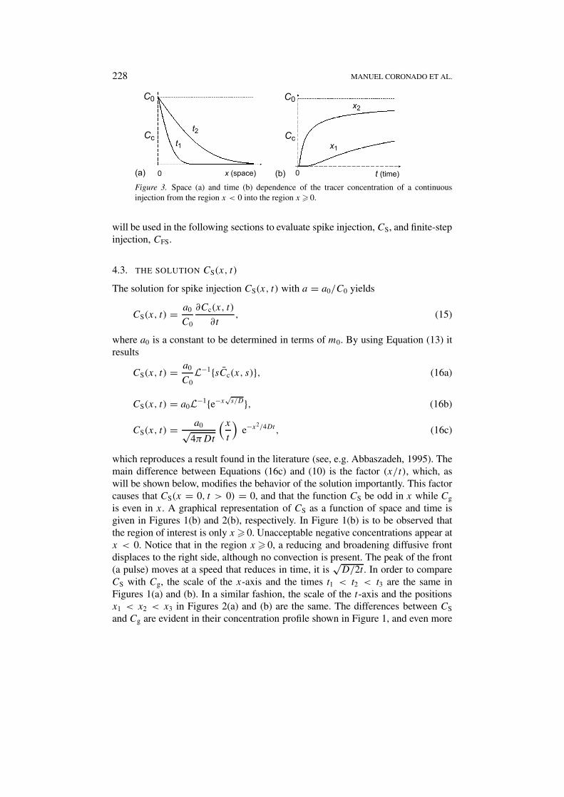
In order to apply the ideas previously discussed, we consider the well-known caseof continuous injection of a tracer diffusing from a medium in x < 0 into a mediumin x � 0, subject to the conditions Cc(x � 0, t � 0) = 0, Cc(x < 0, t) = C0 andCc(x → ∞, t) = 0 (see, e.g. Crank, 1956 or Bear, 1972). The solution in Laplacespace is given by

Cc(x, s) = C0

se−x

√s/D, (13)

and in real space given by the following expression

Cc(x, t) = C0 erfc

(x√4Dt

). (14)

The space dependence of Cc(x, t) for two different times, t1 < t2 is shownin Figure 3(a) and its time behavior at two positions x1 < x2 is illustrated inFigure 3(b). The tracer is diffusing from the region x < 0 into the region x � 0.At a given position x, the tracer concentration starts increasing at the breakthroughtime and asymptotically reaches C0. The previously discussed analytical results


Figure 3. Space (a) and time (b) dependence of the tracer concentration of a continuousinjection from the region x < 0 into the region x � 0.

will be used in the following sections to evaluate spike injection, CS, and finite-stepinjection, CFS.

4.3. THE SOLUTION CS(x, t)

The solution for spike injection CS(x, t) with a = a0/C0 yields

CS(x, t) = a0

C0

∂Cc(x, t)

∂t, (15)

where a0 is a constant to be determined in terms of m0. By using Equation (13) itresults

CS(x, t) = a0

C0L−1{sCc(x, s)}, (16a)

CS(x, t) = a0L−1{e−x√

s/D}, (16b)

CS(x, t) = a0√4πDt

(x

t

)e−x2/4Dt, (16c)

which reproduces a result found in the literature (see, e.g. Abbaszadeh, 1995). Themain difference between Equations (16c) and (10) is the factor (x/t), which, aswill be shown below, modifies the behavior of the solution importantly. This factorcauses that CS(x = 0, t > 0) = 0, and that the function CS be odd in x while Cg

is even in x. A graphical representation of CS as a function of space and time isgiven in Figures 1(b) and 2(b), respectively. In Figure 1(b) is to be observed thatthe region of interest is only x � 0. Unacceptable negative concentrations appear atx < 0. Notice that in the region x � 0, a reducing and broadening diffusive frontdisplaces to the right side, although no convection is present. The peak of the front(a pulse) moves at a speed that reduces in time, it is

√D/2t . In order to compare

CS with Cg, the scale of the x-axis and the times t1 < t2 < t3 are the same inFigures 1(a) and (b). In a similar fashion, the scale of the t-axis and the positionsx1 < x2 < x3 in Figures 2(a) and (b) are the same. The differences between CS

and Cg are evident in their concentration profile shown in Figure 1, and even more


noticeable in the region near x = 0. At this point a maximum in the pulse isexpected, as in Cg, however CS becomes zero there, what is clearly incorrect. Thedifferences between CS and Cg are however not so apparent in the breakthroughcurves in Figure 2, where the curves are essentially similar (the narrower pulsesseen in CS can be attributed to other phenomena, such as a larger diffusion). Thissimilarity has been probably the main cause of possible misinterpretation of tracertest data, not realizing that the model has improper boundary conditions.

In the next few paragraphs we calculate and analyze some properties of CS

that quantitatively show it is not a physically correct solution. These propertiesare: initial condition, total mass inside the reservoir region and total mass flowingthrough a cross section. The initial condition satisfied by CS(x, t) can be obtainedfrom Equation (16c), it is

CS(x, 0) = −2a0Dd[δ(x)]

dx. (17)

This expression has been derived from a mathematical expression for the Diracdelta (Arfken, 1970), δ(x) = limn→∞(n/

√π) exp (−n2x2). To see how this

expression appears, we derive δ(x) with respect to x. It follows d[δ(x)]/dx =limn→∞ (−2n3x/

√π) exp (−n2x2). After substitution of n by 1/

√4Dt and com-

parison with Equation (16c), it yields Equation (17). Roughly seen graphically,the function d[δ(x)]/dx is zero at x = 0, antisymmetric in x, infinite around 0+,and zero as x → ∞. Thus, this initial condition inherited from the continuousinjection case differs importantly from what we would expect for the injection of apulse, which is a high and narrow pulse centered at x. This is the case of the initialcondition satisfied by Cg in Equation (10), that is, Cg(x, 0) = (MI/A)δ(x).

The integral∫ +∞−∞ C(x, t) dx gives MI/A for Cg and zero for CS, due to its

antisymmetry in x. However, the total tracer mass inside the region of interest,∫ ∞0 CS(x, t) dx, results from Equation (A.1c) in Appendix A, and Equation (13)∫ ∞

0CS(x, t) dx = a0

C0L−1

{s

∫ ∞

0

C0

se−x

√s/D dx

}, (18a)

∫ ∞

0CS(x, t) dx = a0L−1

{s

(1

s√

s/D

)}, (18b)

∫ ∞

0CS(x, t) dx = a0

√D

πt. (18c)

This means that the total tracer mass in the region x = (0,∞) is not conserved, itdecreases with time as indicating by (18c). This result is physically unacceptable.The total mass in the full space (−∞,∞) is of course mathematically conserved,but equal to zero. The reason why the mass m0 is not conserved grounds on themisleading boundary condition at the origin, CS(x = 0, t > 0) = 0. This conditionyields ∂CS/∂x �= 0 at x = 0, and therefore, accordingly to Equation (7) with


v = 0, there is a diffusive mass flow going to the left side, outside the region ofinterest (0,∞); this unexpected and spurious flow causes m0 to decrease.

If the total mass in Equation (18c) were constant, Equation (5) would be acondition to determine the constant a0 in terms of the total injected mass m0.

On the other hand, the cumulative tracer mass that flows through a cross-section,A, located at x > 0 results zero, as can be calculated from Equation (A.4) inAppendix A:

mJ

A=

∫ ∞

0Jx dt = −D

[∂(a0 e−x

√s/D)

∂x

]s=0

= 0. (19)

This strange result is a consequence of the improper properties of CS. It is phys-ically wrong, although it is mathematically correct, since only diffusive flow ispresent, which is given by −D∂C/∂x. It could be mathematically explained byobserving that in the region at the right side of the pulse maximum in the regionx � 0 (see Figure 1(b)) the slope is negative and thus there is a diffusive massflow to the right. In the region at the left side of the pulse maximum and for x � 0the slope is positive, and the flow points to the left. Thus, as the diffusive pulsego through a cross-section located at any x > 0 there appear first a mass flowto the right and then a flow to the left, the net balance gives zero, as obtained inEquation (19). This result differs from the result for Cg in Equation (12), where mJ

is half of the total injected mass, as physically expected.We conclude that solution Cg(x, t) gives physically correct results since the

total tracer mass in the region of interest (0,∞) keeps constant, m0, and the totaltracer mass going through a cross-section results m0, as expected. On the otherhand, CS(x, t) in Equation (16c) is physically unacceptable and should not be usedto model tracer spike injection.

The mathematical difference between the acceptable solution of Equation (10)and the solution in Equation (16c) rests in the factor (x/t). There is an incor-rect statement found in the literature that sets the factor (x/t) in Equation (16c)equal to a constant (e.g. Abbaszadeh, 1995). In this case, the inadequate solu-tion CS in Equation (16c) would result into an acceptable solution of the typeCg, in Equation (10). The argument to set (x/t) equal to a constant, invokes amoving frame of reference with constant speed u, on which u = x/t holds. Thisis however not possible: a correctly performed coordinate transformation from x

to x′ = x − ut would yield x/t → (x′/t + u). On the other hand, introducingx = ut in Equation (16c) it would yield the concentration seen by an observertraveling at speed u, and located at the origin on the moving frame of reference, itis C(x′ = 0, t) = (a0u/

√4πDt) e−u2t/D. This concentration is different from what

would be seen at a given fixed position x. Furthermore, the diffusive pulse travelsat a non-constant speed,

√D/2t , and therefore the pulse speed cannot be taken as

the constant speed u of the moving frame of reference. It should be mentioned, thatthe solution finally employed in the document referred above (Abbaszadeh, 1995)is correct, although the arguments to derive it are incorrect.


4.4. FINITE-STEP INJECTION

In order to model the diffusion of a pulse produced by a finite-step injection, weconsider a solution of the type in Equation (3), with b = aFS/(�t)C0 to get

CFS(x, t;�t) = aFS

(�t)C0[Cc(x, t) − Cc(x, t − �t)], (20)

together with condition Cc(x � 0, t � 0) = 0. The factor aFS is a free constant to bedetermined in terms of the total tracer mass injected in the reservoir, that is, throughEquation (5). The factor 1/�t has been included in order to reproduce CS(x, t) inthe limiting case �t → 0. Figure 4 graphically illustrates how the solution CFS

results from the superposition of two shifted continuous injection solutions Cc. InFigure 4(a) the curve Cc(x, t − �t) should be subtracted from Cc(x, t) to yield thesuperposition curve, CFS(x, t), shown in Figure 4(b). In the limiting case �t → 0the curves reproduce those in Figure 2(b).

By substituting Equation (14) in expression (20), and using the definition of thecomplementary error function it results, for t � �t

CFS(x, t;�t) = 2aFS√π(�t)

∫ x/√

4D(t−�t)

x/√

4Dt

e−ξ2dξ. (21)

For 0 � t � �t the upper limit in the integral of Equation (21) should be ∞. SeeFigure 5 for an illustration of the behavior of the function CFS. Figure 5(a) showsthat a diffusive front leaves the vertical axis at t = �t and spreads moving to theright side. For t > �t it holds CFS(x = 0, t) = 0. This condition is equivalentto the condition found in Section 4.3 regarding CS, and its appearance here it is

Figure 4. Illustration of how finite-step injection is built up from the superposition of twocontinuous injection functions. In (a) two identical functions, just shifted in the time by �t ,are plotted. In (b) the resulting finite-step concentration, obtained from the subtraction of thefunctions in (a), is shown.


Figure 5. Space (a) and time (b) behavior of the finite-step injection CFS resulting from theCc shown in Figure 3. Here t1 < t2 < t3 with t1 < �t < t2, and x1 < x2 < x3. For t ��t

notice in plot (a) that CFS is zero at x = 0.

an indication of a problem of mass conservation similar to the problem discussedin that section, as will be shown below. As might be expected, for t > �t thecurves in Figure 5(a) reproduce the curves in the region x > 0 of Figure 1(b).Figure 5(b) describes the behavior of CFS as a function of time for a fixed position.These curves are similar to curves in Figure 2(b).

For the case t � �t together with �t � 8Dt2/x2 expression (21) can beapproximated by

CFS(x, t;�t) = aFS√4πDt

{x

te−x2/4Dt

[1 + �t

2t

(3

2− x2

4Dt

)+

+ O(

�t

t

)2 ]}. (22)

In the limiting case �t → 0 Equation (22) simplifies to Equation (16c), that is, thespike case, as expected. The total amount of tracer in the reservoir at time t > �t

is obtained from expression (5). It is

∫ ∞

0CFS(x, t;�t) dx = aFS

√D

πt

[1 + �t

4t+ O

(�t

t

)2]

, (23)

which gives Equation (18c) in the limiting case �t → 0. Notice that although astep input of mass is entering the region, the total mass inside the region reduceswith time. The problems found with CFS are similar to the problems seen beforewith CS. Thus the superposition method, expression (20), does not yield adequatemodels for step-injection.


4.5. BRIEF COMMENTS REGARDING CONVECTION

Let us very briefly present and discuss the results that may appear when convectionis taken into account.

The solution of Equation (1) subject to condition Cg(x, 0) = (MI/A)δ(x) is(see, e.g. Bear, 1972, p. 628):

Cg(x, t) = MI/A√4πDt

e−(x−vt)2/4Dt . (24)

The solution obtained from the time derivative shown in Equation (2) with Cc thecontinuous injection (see, e.g. Bear, 1972, p. 630 or Abbaszadeh, 1995, p. 438)given by Cc(x, t) = (C0/2)[erfc((x − vt)/

√4Dt) + evx/D erfc((x + vt)/

√4Dt)]

results to be:

CS(x, t) = a1√4πDt

(x

t

)e−(x−vt)2/4Dt, (25)

where a1 = aC0 is a constant to be determined, in principle, in terms of the totaltracer mass injected in the reservoir, which should keep constant. However, due tothe presence of the factor (x/t) the solution presents mass conservation problemssimilar to those discussed in Section 4.3 for the case without convection. It appearsagain the physically incorrect condition CS(x = 0, t > 0) = 0.

A plot of the solutions Cg and CS from expressions (24) and (25) is given inFigures 6(a) and (b), respectively. The scale in the x-axis as well as the timest1 < t2 < t3 take the same values in both plots. A diffusive pulse moving to theright side can be recognized in both figures. However CS is negative for x < 0and CS = 0 at x = 0. It can be shown that the area below the curves in (b) forthe full region x = (−∞, ∞) is constant, as it is also the case for the curves in(a), but the tracer mass in the reservoir, that is, x = (0,∞), increases with timein case (a) due to the motion of the incoming pulse, and reduces in case (b) due tothe mass lost associated to the diffusive flow going outside the reservoir, through

Figure 6. Diffusion and convection of a pulse resulting (a) from a Dirac delta at t = 0, and(b) from the time derivative CS of a continuous injection. This figure is a generalization ofFigure 1 to the case v �= 0.


the boundary at x = 0. The difference between Cg and CS are very significantaround x = 0 and particularly for short times, however for large times and due toconvection (see, e.g. the corresponding plot for t3) the concentration profiles arequalitatively similar. Anyway, the problems due to the wrong boundary conditionset at x = 0 prevail when convection is present.

4.6. SOME IMPORTANT REMARKS ON OTHER INITIAL AND BOUNDARY

CONDITIONS MENTIONED IN THE LITERATURE

In the tracer literature it is frequently found (see, e.g. the summary in Table 24 ofKass, 1998, p. 376) that pulse injection tests in semi-infinite reservoirs are modeledby posing the condition C(x = 0, t) = aδ(t), where a is a constant. Unfortunately,this condition reproduces the inappropriate condition discussed along this paper,C(x = 0, t > 0) = 0, and yields solutions that might show inadequate tracerdiffusive flows going outside the reservoir at x = 0 (and therefore might lead tono mass conservation!). A better way to model a pulse injection test is through theinitial condition mentioned in Section 4.1, that is, C(x, t = 0) = (MI/A)δ(x),which includes the commonly employed initial condition C(x �= 0, t = 0) = 0.

It is also important to be mentioned that some authors, see, for example,Brigham (1974), Kreft and Zuber (1978, 1986), Parker and van Genuchten (1984,1986), use the so-called flow concentration or flux-averaged concentration, Cf ≡Jx/v = C − (D/v)∂C/∂x to properly describe boundary conditions in laboratorycore tracer tests. It should be pointed out that Cf is a linear combination of thefunctions C and ∂C/∂x, and therefore Cf satisfies Equation (1), accordingly towhat is stated in Section 2. Due to its definition, setting boundary and initial condi-tions in terms of Cf, is equivalent to setting conditions on the mass flow Jx . Thus,the finite-step condition imposed to Cf: Cf(x = 0+) = C0 for 0 < t � �t andCf(x = 0+) = 0 for t > �t has a different physical meaning than the misleadingconditions set on C and discussed in this paper. The condition on Cf is a step-size condition on the injection flow, which is different from a step-size on theconcentration. Therefore the problems discussed in this paper do not apply to Cf.

5. Final Remarks and Conclusions

The employment of the commonly used methodology questioned in this paperis not recommendable. The methodology models spike injection by the functionobtained from the time derivative of the solution corresponding to continuous injec-tion. Further, it models finite-step injection by the superposition of two continuousinjection solutions displaced in time. We have shown here, for the case of a one-dimensional tracer pulse diffusing in a homogeneous semi-infinite reservoir withno tracer loss mechanisms present, that solutions obtained by this mathematicalmethodology have serious problems regarding mass conservation. The origin of theproblems grounds on the physically inappropriate boundary conditions satisfied bythese solutions. Specifically, a wrong condition states that the tracer concentration


at the injection site and reservoir inner boundary, x = 0, should be zero at anytime immediately after the injection ends. This condition gives rise to incorrectdiffusive flows going outside the reservoir, and thus reducing the tracer mass init. In order to emphasize the misleadings involved in the condition, the solutionis compared against a genuine (rigorous) solution obtained by a direct solvingmethod, where appropriate boundary conditions are posed. Important differencescan be observed in space concentration profiles close to the injection site, wherethe improper boundary conditions at x = 0 yields no tracer, precisely where amaximum in the concentration is expected. The situation looks different when thetracer breakthrough curves are analyzed. Here the curves result essentially sim-ilar and the effect of the wrong posed boundary conditions is not immediatelyvisible. This fact has been probably the cause of possible misinterpretations offield or laboratory data. If spatial tracer distributions were available, the differencesbetween the models would possibly immediately appear.

A central recommendation to model spike and finite-step tracer injection isto avoid the use of solutions obtained from the methodology criticized in thispaper. Use solutions obtained from methods that allow posing appropriate initialand boundary conditions. Care should be taken when employing the conditionC(x = 0, t) = aδ(t), a being a constant, since it might lead to a physically wrongcondition. It is worthwhile to mention that numerical approaches employed to treatmore complex practical tracer test cases do not have the problem mentioned in thispaper. They numerically solve the equations from its basic differential form, posinginitial and boundary conditions explicitly. Of course, these conditions should bephysically meaningful.

Appendix A. Formula to Evaluate mmm0 and mmmJJJ

In order to analyze mass conservation in a half space reservoir, the quantities m0

and mJ defined in Equations (5) and (6) are needed. There are different ways toevaluate them, one of these ways is the direct method (analytically or numerically),which requires the calculation of C(x, t) and then the evaluation of the integrals inEquations (5) and (6), what in general is cumbersome. However, by taking advan-tage of the origin of CS(x, t) we can evaluate m0 in a simpler form. Using someproperties of the Laplace transform, the evaluation of mJ can also become easier.A procedure to perform these calculations is shown below.

A.1. m0 FOR SPIKE INJECTION, CS

The calculation of m0 in Equation (5) can be simplified, if the Laplace transformof the concentration for the continuous injection problem is known, Cc(x, s), here,s is the Laplace conjugate variable of t . In this case∫ ∞

0CS dx = a

∫ ∞

0L−1

{L

{∂Cc(x, t)

∂t

}}dx, (A.1a)

236 MANUEL CORONADO ET AL.∫ ∞

0CS dx = a

∫ ∞

0L−1 {sCc(x, s) − Cc(x, t = 0)} dx, (A.1b)

∫ ∞

0CS dx = aL−1

{s

∫ ∞

0Cc(x, s) dx −

∫ ∞

0Cc(x, 0) dx

}, (A.1c)

here L means Laplace transform. The assumption limt→0 Cc(x, t) e−st = 0 wasmade. In general, the continuous injection problems treated in the literature con-sider Cc(x � 0, t = 0) = 0; thus the second term in the RHS of Equation (A.1c)disappears. Frequently the integral

∫ ∞0 Cc(x, s) dx and the inverse Laplace trans-

form involved are easier to calculate than the integral∫ ∞

0 Cs(x, t) dx.Condition (A.1c), with m0 being a constant, would imply in this case that∫ ∞

0Cc(x, s) dx = f (x)

s2, (A.2)

where f (x) is a function of x. In the case without convection, condition (A.2)guarantees the conservation of tracer mass injected in the reservoir region (0,∞).If it is not constant, CS(x, t) is not a physically correct solution, and should not beused in the description of tracer flow. On the other hand, if convection is present,condition above should be tested using the solution in the limiting case v → 0.

A.2. FLOW THROUGH A CROSS-SECTION, mJ

We can evaluate the cumulative tracer flow through a cross-section, A, perpendic-ular to the direction of flow, by observing that the integral in Equation (8) can bewritten as∫ ∞

0C(x, t) dt =

[∫ ∞

0C(x, t) e−st dt

]s=0

= C(x, s = 0). (A.3)

Thus, from Equation (8) it follows that

mJ

A= −D

[∂C(x, s)

∂x

]s=0

+ vC(x, 0). (A.4)

In general, this last expression (A.4) is easier to evaluate than expression (8). In thecase without convection the conservation of the tracer mass implies mJ = MI/2.If the injected pulse goes inside the region 0 � x � ∞ due to convection, thenmJ = MI would be expected.

References

Abbaszadeh, M.: 1995, Appendix in the book, in: B. Zemel, (ed.), Tracers in the Oil Field, Elsevier,New York, pp. 429–440.

Arfken, G.: 1970, Mathematical Methods for Physicists, Academic Press, New York, pp. 413–419.


Bear, J.: 1972, Dynamics of Fluids in Porous Media, Dover Publications, New York, pp. 627–634.Brigham, W. E.: 1974, Mixing equations in short laboratory columns, Soc. Pet. Eng. J. 14, 91–99.Coats, K. H.: 1963, Dead-end pore volume and dispersion in porous media, in: Annual SPE Fall

Meeting, New Orleans, USA, October 6–9, 1963, SPE Paper 647.Crank, J.: 1956, The Mathematics of Diffusion, Oxford University Press, London, pp. 9–25.Kass, W.: 1998, Tracing Technique in Geohydrology, A. A. Balkema, Rotterdam, pp. 341–356.Kreft, A. and Zuber, A.: 1978, On the physical meaning of the dispersion equation and its solutions

for different initial and boundary conditions, Chem. Eng. Sci. 33, 1471–1480.Kreft, A. and Zuber, A.: 1986, Comment on “Flux-Averaged and Volume-Averaged Concentrations

in Continuum Approaches to Solute Transport”, by J. C. Parker and M. Th. van Genuchten, WaterResour. Res. 22, 1157–1158.

Parker, J. C. and van Genuchten, M. Th.: 1984, Flux-averaged and volume-averaged concentrationsin continuum approaches to solute transport, Water Resour. Res. 20, 866–872.

Parker, J. C. and van Genuchten, M. Th.: 1986, Reply, Water Resour. Res. 22, 1159–1160.Ramırez, J., Rivera, J., Samaniego, F. and Rodrıguez, F.: 1990, A semi analytical solution for tracer

flow in naturally fractured reservoirs, Fifteenth Workshop on Geothermal Reservoir Engineering,Stanford University, Stanford, CA, January 23–25, 1990.

Ramırez, J., Samaniego, F. Rodrıguez, F., and Rivera, J.: 1995, Tracer test interpretation in naturallyfractured reservoirs. SPE Paper 28691, SPE Formation Evaluation J., 19–25.

Tang, D. H., Frind, E. O. and Sudicky, E. A.: 1981, Contaminant transport in fractured porous media:analytical solution for a single fracture, Water Resour. Res. 17, 555–564.

Walkup Jr., G. W. and Horne, R. N.: 1985, Characterization of tracer retention process and their effecton tracer transport in fractured geothermal reservoirs, SPE 1985 California Regional Meeting,Bakersfield, CA, March 27–29, 1985, SPE Paper 13610.

New Considerations on Analytical Solutions Employed in Tracer Flow Modeling

Documents

Transcript of New Considerations on Analytical Solutions Employed in Tracer Flow Modeling