Neural Aerial Social Force Model: Teaching a Drone to ...

FACULTAT D’INFORMÀTICA DE BARCELONA (FIB)FACULTAT DE MATEMÀTIQUES (UB)

ESCOLA TÈCNICA SUPERIOR D’ENGINYERIA (URV)UNIVERSITAT POLITÈCNICA DE CATALUNYA (UPC)

UNIVERSITAT ROVIRA I VIRGILI (URV)UNIVERSITAT DE BARCELONA (UB)

MASTER THESIS

Neural Aerial Social Force Model: Teaching a Drone toAccompany a Person from Demonstrations

Author:Carles COLL GOMILA

Supervisors:Dr. René ALQUÉZAR

MANCHODra. Anaís GARRELL

ZULUETA

A thesis submitted in fulfillment of the requirementsfor the degree of Master in Artificial Intelligence

in the

Barcelona School of Informatics

October 15, 2018

iii

To my parents, Toni Coll Oliver and Virgina GomilaMartínez, and my sister Maria Cristina, who are always

in my thoughts.

v

AcknowledgementsFirst and foremost, I want to thank my parents, because this thesis wouldn’texist without their constant support. I also want to thank my advisors, Dra.Anaís Garrell and Dr. René Alquézar, for proposing me the current thesis,and always supporting me and giving me their expert advice when it wasmost needed. Lastly, thanks to Fernando Herrero for his always kindly andtireless help during the experiments carried out in this work.

vii

UNIVERSITAT POLITÈCNICA DE CATALUNYA (UPC)

AbstractBarcelona School of Informatics

Master in Artificial Intelligence

Neural Aerial Social Force Model: Teaching a Drone toAccompany a Person from Demonstrations

by Carles COLL GOMILA

Recent advances in computing power, sensor technology and battery du-ration, have motivated the development of commercial Unmanned AerialVehicles (UAV), most commonly found in the form of quadrotors. Quadro-tors have never been so cheap and easier to manufacture, which makesavailable to the wide public. Although commercial drones are in generalnot very sophisticated, they are incredibly versatile, and there is a hugepotential of applications in which they could be deployed in the future.

However, there are some technical aspects that prevent this from hap-pening right now. While the hardware technologies found in UAVs areadvanced, software technologies have still quite a long distance to reachthe hardware’s level. One of the main issues, which is still not success-fully solved, is the task of navigation. Robot navigation is one of the great-est challenges in Robotics, and particular case of aerial navigation is evenharder. On one side, Aerial robots must deal with an extra dimension ofmovement, and on the other side, there is little research about this topicbecause aerial robots haven’t been considered traditionally.

In consequence, there has been a recent increment in the effort dedi-cated to the development of new navigation techniques for UAVs. Some ofthese techniques are modifications of existing ones, which adapt older tech-niques to the new requirements of aerial robots, while others are completelynew. However, all of these have in common the consideration of social in-teractions with humans. Due to the availability and potential of UAVs, it isexpected to find aerial robots doing all kinds of tasks with humans. There-fore, there is a need to improve the way drones interact with people, so thathumans feel safe and comfortable around them. In the present work, wefocus on the robot companion problem, and present a solution for the prob-lem of a drone that flies in a side-by-side formation with a person in a socialand safe manner.

The presented navigation technique consists of a system that is ableto autonomously control a drone so that it accompanies a human that ismoving in a real environment. The drone avoids obstacles and maintains acertain distance to the person, which perceived by the human as safe andsocially engaging. This navigation method is based on the Artificial Po-tential Fields (APF) framework in the sense that interactive forces are usedto describe the state of the world. However, the novelty introduced in thepresented technique lies in the introduction of a non-linear model to com-pute the motion of the drone from the description of the world. A Neural

viii

Network is used to compute acceleration commands, which takes as inputthe interactive forces. The neural Neural Network, which is the core of thenavigation method, is trained on data recorded from trajectories providedby a human expert.

The task of recording example trajectories is performed in a simulator,where the human expert is in control of the drone and tries to accompany asimulated human while avoiding obstacles. Several types of environmentswith different degrees of complexity have been generated, with the aim todivide the task of learning a control policy in different stages. In each stage,a given environment type is chosen, expert trajectories are recorded, and adataset is built by extracting the defined features. These features are basedon the original APF framework and include some minor modifications thathave shown improved performance. With the built dataset it is then possi-ble to train, validate and test several Machine Learning models.

Moreover, the system is reinforced with a human path prediction mod-ule to improve the drone’s navigation, as well as, a collision detection mod-ule to completely avoid possible impacts. The human path prediction mod-ule is based on a neural network that predicts the future position of thehuman 1 second into the future. This module provides the drone with anestimate of the path followed by the human and allows it to fly more nat-urally, as if it knew the intention of the human. The collision detectionmodule is there to add an additional safety layer in case the learned policyfails at avoiding an obstacle.

A new quantitative metric of performance for the task we aim to achieveis introduced in the present work. This metric is based on the idea of prox-emics and defines three concentric spherical volumes around the main hu-man, each one providing a different score. The final performance value iscomputed as a weighted intersection of the volume of the drone with thedifferent spherical regions. This metric provides a quantitative estimate ofthe performance achieved by the learned policies, and can be measured inany simulated environment.

Finally, we present experimental evidence about the degree in whichthe defined problem has been solved. On the one hand, test simulationshave been performed in order to check that the learned policies exhibit anappropriate behaviour when they are controlling the drone in unseen simu-lated environments. The previous metric of performance is used, providinga quantitative comparison between the different Machine Learning modelstested. On the other hand, the best policy, according to the results obtainedin the test simulations, is implemented in the real drone and tested on a realenvironment, in this case the Mobile Robotics laboratory.

Results form test simulations prove that it is possible to learn controlpolicies from expert demonstrations in simulated environments that be-have correctly when run in simulated environments. Real experiments,however, show that the policies learned in simulated environments fail atthe task of controlling a real drone. This result is not unexpected becausethe policies are trained in simulated environments, which are simplifica-tions of reality. The simulator used to train the models does not have anykind of physics engine, therefore, the dynamics of the drone are ignored.Also, in a real setup, sensors have significant noise and the drone suffersfrom drift and is unable to perform the motion commands with completeaccuracy. Essentially, the policies are trained under conditions that do not

ix

match real conditions, which results in a rough transition from simulator toreal life.

xi

Contents

Acknowledgements v

Abstract vii

1 Introduction 11.1 Motivation . . . . . . . . . . . . . . . . . . . . . . . . . . . . . 21.2 Objectives . . . . . . . . . . . . . . . . . . . . . . . . . . . . . 31.3 Main Contributions . . . . . . . . . . . . . . . . . . . . . . . . 3

1.3.1 Derived Publications . . . . . . . . . . . . . . . . . . . 4

2 State of the Art 52.1 Human-Drone interaction . . . . . . . . . . . . . . . . . . . . 52.2 Social Drone Navigation . . . . . . . . . . . . . . . . . . . . . 6

2.2.1 Robot Collision Avoidance . . . . . . . . . . . . . . . 72.2.2 Human Motion Prediction . . . . . . . . . . . . . . . . 9

3 Aerial Social Navigation 113.1 Introduction . . . . . . . . . . . . . . . . . . . . . . . . . . . . 113.2 Artificial Potential Fields . . . . . . . . . . . . . . . . . . . . . 11

3.2.1 Attraction Force . . . . . . . . . . . . . . . . . . . . . . 123.2.2 Repulsion Force . . . . . . . . . . . . . . . . . . . . . . 13

3.3 Social Force Model . . . . . . . . . . . . . . . . . . . . . . . . 143.4 Aerial Social Force Model . . . . . . . . . . . . . . . . . . . . 15

3.4.1 Online Regression Model for Human Path Prediction 153.4.2 Interactive forces definition . . . . . . . . . . . . . . . 173.4.3 Goal attraction force . . . . . . . . . . . . . . . . . . . 183.4.4 Robot-object interaction force . . . . . . . . . . . . . . 183.4.5 Robot-human interaction force . . . . . . . . . . . . . 183.4.6 Quantitative Metrics . . . . . . . . . . . . . . . . . . . 20

4 Data Generation and Feature Definition 234.1 Expert Trajectories Generation . . . . . . . . . . . . . . . . . . 23

4.1.1 Training, Validating and Testing the models . . . . . 244.1.2 The simulator . . . . . . . . . . . . . . . . . . . . . . . 254.1.3 The simulated environments . . . . . . . . . . . . . . 254.1.4 Open space without static obstacles and bots (AB) . . 264.1.5 Open space with bots and without static obstacles (D) 264.1.6 Open space with static obstacles and without bots (KL) 274.1.7 Test environment with static obstacles and without

bots (M) . . . . . . . . . . . . . . . . . . . . . . . . . . 284.1.8 Test environment with static obstacles and bots (C) . 294.1.9 Space replicating laboratory conditions (Lab) . . . . . 294.1.10 Technical details about environment generation . . . 30

4.2 Feature Definition . . . . . . . . . . . . . . . . . . . . . . . . . 31

xii

4.2.1 Companion Attractive Force . . . . . . . . . . . . . . 324.2.2 Goal Attractive Force . . . . . . . . . . . . . . . . . . . 324.2.3 Static Object Repulsive Force . . . . . . . . . . . . . . 324.2.4 Pedestrian Repulsive Force . . . . . . . . . . . . . . . 334.2.5 Drone Velocity Feature . . . . . . . . . . . . . . . . . . 34

5 Additional Requirements 355.1 Human Path Prediction . . . . . . . . . . . . . . . . . . . . . 35

5.1.1 Dataset of human paths . . . . . . . . . . . . . . . . . 355.1.2 Human path prediction models . . . . . . . . . . . . . 375.1.3 Training and testing the models . . . . . . . . . . . . 40

5.2 Collision Detection . . . . . . . . . . . . . . . . . . . . . . . . 415.2.1 Dataset of drone collisions . . . . . . . . . . . . . . . . 425.2.2 Collision detector model . . . . . . . . . . . . . . . . . 44

5.3 Quantitative metric of performance . . . . . . . . . . . . . . . 46

6 Learned Models 516.1 The models . . . . . . . . . . . . . . . . . . . . . . . . . . . . . 51

6.1.1 Linear Regression . . . . . . . . . . . . . . . . . . . . . 526.1.2 Artificial Neural Networks . . . . . . . . . . . . . . . 52

6.2 Learning a flying policy in open space with no obstacles andno pedestrians . . . . . . . . . . . . . . . . . . . . . . . . . . . 546.2.1 The dataset . . . . . . . . . . . . . . . . . . . . . . . . 546.2.2 Detailed description of the tested models . . . . . . . 556.2.3 Testing procedure . . . . . . . . . . . . . . . . . . . . . 566.2.4 Training Results . . . . . . . . . . . . . . . . . . . . . . 59

6.3 Learning a flying policy in open space with only pedestrians 596.3.1 The dataset . . . . . . . . . . . . . . . . . . . . . . . . 606.3.2 Evaluating the models . . . . . . . . . . . . . . . . . . 60

6.4 Learning a flying policy in a space populated with obstacles 626.4.1 The dataset . . . . . . . . . . . . . . . . . . . . . . . . 626.4.2 Description of the models . . . . . . . . . . . . . . . . 636.4.3 Evaluating the models and results . . . . . . . . . . . 64

6.5 Learning a flying policy in laboratory space . . . . . . . . . . 666.5.1 The dataset . . . . . . . . . . . . . . . . . . . . . . . . 666.5.2 Evaluating the models . . . . . . . . . . . . . . . . . . 66

7 Hardware and Software 717.1 AR.Drone 2.0 . . . . . . . . . . . . . . . . . . . . . . . . . . . 71

7.1.1 Mechanical details . . . . . . . . . . . . . . . . . . . . 717.2 Optitrack . . . . . . . . . . . . . . . . . . . . . . . . . . . . . . 727.3 Software . . . . . . . . . . . . . . . . . . . . . . . . . . . . . . 73

7.3.1 FreeGLUT . . . . . . . . . . . . . . . . . . . . . . . . . 737.3.2 Robot Operating System . . . . . . . . . . . . . . . . . 747.3.3 Gazebo . . . . . . . . . . . . . . . . . . . . . . . . . . . 757.3.4 TUM Simulator . . . . . . . . . . . . . . . . . . . . . . 757.3.5 Final NASFM architecture . . . . . . . . . . . . . . . . 75

xiii

8 Results 798.1 Results from simulations . . . . . . . . . . . . . . . . . . . . . 79

8.1.1 Policy learned in open space with no obstacles and nopedestrians . . . . . . . . . . . . . . . . . . . . . . . . 79

8.1.2 Policy learned in open space with only pedestrians . 808.1.3 Policy learned in open space populated with obstacles 818.1.4 Policy learned in spaces replicating laboratory condi-

tions . . . . . . . . . . . . . . . . . . . . . . . . . . . . 828.1.5 Conclusion . . . . . . . . . . . . . . . . . . . . . . . . 83

8.2 Results from real experiments . . . . . . . . . . . . . . . . . . 838.2.1 Implementation of the model on the AR.Drone . . . . 848.2.2 Simulating lab policy in Gazebo . . . . . . . . . . . . 848.2.3 Running the control policy on the real drone . . . . . 85

9 Conclusions 879.1 Learning and effective policy for simulated environments . . 879.2 Learning and effective policy for a real drone . . . . . . . . . 889.3 Final conclusions . . . . . . . . . . . . . . . . . . . . . . . . . 89

10 Future work 9110.1 Limitations of the current work . . . . . . . . . . . . . . . . . 9110.2 Next steps . . . . . . . . . . . . . . . . . . . . . . . . . . . . . 92

xv

List of Figures

3.1 Uncertainty zone: The Uncertainty zone is represented as acylindrical area with radius r and height h. This picture isextracted from L. Garza [15]. . . . . . . . . . . . . . . . . . . . 13

3.2 3D view of the anisotropic factor. The top row shows thehuman’s anisotropic factor when the parameters λRj = 0.25and ξRj = 0.25. The bottom row shows the anisotropic factorfor the drone, when λRj = 0.9 in (E) and (F) and when ξRj =0.5 in (G) and (H) . . . . . . . . . . . . . . . . . . . . . . . . . 20

4.1 Cropped screenshot from the simulator view for a type B en-vironment. The visible elements are: the companion (greenlegoman), the drone and the goal (green cylinder). The redcircle on the floor is the predicted companion position onesecond into the future. . . . . . . . . . . . . . . . . . . . . . . 27

4.2 Cropped screenshot from the simulator view for a type Denvironment. The visible elements are: the companion, thedrone, the current goal and the bots (red legomen). . . . . . 27

4.3 Cropped screenshots from the simulator view for a type K(left) and type L (right) environments. Left: the visible el-ements are the drone, the companion, the goal and the col-umn. Right: the visible elements are the drone, the compan-ion, the bridge on the front and the column on the back. Thegoal is occluded by the column. . . . . . . . . . . . . . . . . . 28

4.4 Frame from the simulator’s view for a type M environment.The visible elements are: the companion, the drone and sev-eral columns and bridges. The goal is out of vision in thedirection the companion is heading to. . . . . . . . . . . . . . 29

4.5 Frame from the simulator’s view for a type C environment.The visible elements are: the companion, the drone, the botsand several trees. The goal is occluded by the trees in thebackground. . . . . . . . . . . . . . . . . . . . . . . . . . . . . 30

4.6 Cropped screenshots from the simulator view for two differ-ent type Lab environments. The available space is signifi-cantly reduced, goals are hidden and the obstacle is shapedlike the obstacles found in the laboratory. . . . . . . . . . . . 31

4.7 Representation of companion and goal attractive force fea-tures. FALTA DIBUIXAR ELS FEATURES. . . . . . . . . . . . 33

xvi

5.1 Schematic description of the neural networks’ architecturesfor the human path prediction task. Left: the three layer NN.Right: the five layer NN. The None in the first component ofeach input and output is the way Keras indicates that thelayer accepts an arbitrarily amount of samples, i.e., it cancompute the output of a single sample or a set of samplesgathered in a matrix. . . . . . . . . . . . . . . . . . . . . . . . 39

5.2 Predicted position increment and true true position incre-ment for each frame in a trajectory fragment. . . . . . . . . . 41

5.3 Two screenshots of the drone collision simulator view illus-trating the shape of the simulated environments. . . . . . . . 43

5.4 Schematic description of the neural networks’ architecturestested for the collision detection task. Left: the two layerNN. Right: the three layer NN. The None in the first com-ponent of each input and output is the way Keras indicatesthat the layer accepts an arbitrarily amount of samples, i.e., itcan compute the output of a single sample or a set of samplesgathered in a matrix. . . . . . . . . . . . . . . . . . . . . . . . 45

5.5 Predicted probability of collision, raw and rounded, com-pared to the target value, for 600 consecutive frames that in-clude 3 collision trajectories from the test set. . . . . . . . . . 47

5.6 Histogram of the distance between the drone and the com-panion for all frames in all recorded expert trajectories. . . . 48

6.1 Illustration of the different terms appearing in equation 6.2 . 536.2 Graphical representation of a neural network with three lay-

ers. An arrow indicates a connection between two neuronsand has a weight associated. . . . . . . . . . . . . . . . . . . . 53

6.3 Schematic description of the neural networks’ architecturestested on data from AB type environments. Left: the threelayer NN. Right: the five layer NN. The None in the firstcomponent of each input and output is the way Keras indi-cates that the layer accepts an arbitrarily amount of samples,i.e., it can compute the output of a single sample or a set ofsamples gathered in a matrix. . . . . . . . . . . . . . . . . . . 57

6.4 Predictions of the models compared to real target for a se-quence of frames in the test set, built from type A expert tra-jectories. The targets correspond to the x component of theacceleration. . . . . . . . . . . . . . . . . . . . . . . . . . . . . 58

6.5 Predictions of the models compared to real target for a se-quence of frames in the test set, built from type D expert tra-jectories. The targets correspond to the x component of theacceleration. . . . . . . . . . . . . . . . . . . . . . . . . . . . . 61

6.6 Division into train, validation and test sets of the datasetbuilt from expert trajectories recorded in K and L type en-vironments. Ki is the set of samples that compose the experttrajectory i recorded in environment type K. A similar nota-tion is used for environments type L. . . . . . . . . . . . . . . 64

6.7 Schematic description of the neural networks’ architecturestested on data from KL type environments. Left: the threelayer NN. Right: the five layer NN. . . . . . . . . . . . . . . . 65

xvii

6.8 Predictions of the models compared to real target for a se-quence of frames in the test set, built from type KL experttrajectories. The targets correspond to the y component ofthe acceleration. . . . . . . . . . . . . . . . . . . . . . . . . . . 67

6.9 Predictions of the models compared to real target for a se-quence of frames in the test set, built from lab-type experttrajectories. The targets correspond to the x component ofthe acceleration. . . . . . . . . . . . . . . . . . . . . . . . . . . 69

7.1 The four fundamental movements the AR.Drone is able toperform by individually setting the speed of the rotors. Themagnitude of the blue arrows depict the speed of the rotor . 72

7.2 Cage structure where the camera sensors are mounted. Notethat the cameras record the scene in the center of the cagefrom different angles. . . . . . . . . . . . . . . . . . . . . . . . 73

7.3 Markers applied to A) the AR.Drone, B) the main human pro-tective gear, and C) the obstacle. . . . . . . . . . . . . . . . . 73

7.4 TUM Simulator functional diagram A) in a simulated envi-ronment and B) with a real drone. . . . . . . . . . . . . . . . . 76

7.5 ROS system architectures: A) when the drone is operated ingazebo simulator and B) when the drone is operated in a realexperiment. . . . . . . . . . . . . . . . . . . . . . . . . . . . . 77

8.1 Simulated environment in gazebo replicating the conditionsfound in the laboratory. The drone, the main human and anobstacle are the only elements in the environment, which isalso limited by the green volume. . . . . . . . . . . . . . . . . 85

8.2 Pictures taken during the real experiments, where the learnedpolicy is tested on the real drone. . . . . . . . . . . . . . . . . 85

xix

List of Abbreviations

IRI Institut de Robotica i Informatica IndustrialSFM Social Force ModelESFM Extended Social Force ModelASFM Aerial Social Force ModelNASFM Neural Aerial Social Force ModelAPF Artificial Potential FieldROS Robot Operating SystemLfD Learning from DemonstrationsPfCA Prediction for CompActionBCM Beam Curvature MethodLCM Lane Curvature MethodUAV Unmanned Aerial VehicleHRI Human Robot InteractionMSE Mean Square ErrorHMP Human Motion PredictionNN Neural NetworkANN Artificial Neural NetworkCNN Convolutional Neural NetworkPS3 Play Station 3TUM Simulator Technical University of Munich Simulator

1

Chapter 1

Introduction

The present work explores the possibility of solving a particular problemin the mobile robotics field by proposing a partially novel approach. Theproposed method is in part inspired by previous research from the SocialNavigation domain, and the novelty lies on the introduction of MachineLearning techniques, in a way that still remains mostly unexploited. Butbefore delving into the exact details of the proposed solution, it is neces-sary to provide a brief introduction to the basic ideas and context of thecurrent work.

The field of Robotics is an interdisciplinary branch of engineering andscience that includes mechanical engineering, electronics engineering, com-puter science, and others. Essentially, it deals with the design, construction,operation, and use of robots, as well as, computer systems for their control,sensory feedback, and information processing. The goal of Robotics is todevelop machines that can substitute humans or replicate human actions.

Mobile Robotics is a sub-field of Robotics that only deals with robotsthat are not fixed to one physical location and can, thus, move freely in anenvironment. This condition introduces several technical difficulties thatmust be addressed in order to build a successful mobile robot. In the scopeof this thesis, two of these issues are of particular interest: Social Naviga-tion and Collision Avoidance. The first deals with the task of navigating inan environment where humans are present. The second, as the name indi-cates, focuses on the study of methods that allow a mobile robot to detectand safely avoid collisions with obstacles, which may be present in an en-vironment.

The goal of this academic work is to teach a drone to safely fly side-by-side with a human. Therefore, the problem we are dealing with involvesideas from Social Navigation and Collision Avoidance. Previous to the de-sign of the current approach, an extensive study of the state of the art forboth Social Navigation and Collision Avoidance has been done. In conse-quence, parts of the presented solution are based on previous works. How-ever, viewed as a whole, the work presented in this thesis is novel.

In the previous description of the problem to be solved, the word teachwas used. The choice for this word was deliberated, so as to indicate thata learning approach was chosen to solve the problem. The last decade haswitnessed huge progress in the field of Machine Learning, motivated bythe advances in computation power. New techniques have been developed

2 Chapter 1. Introduction

that allow computers to reach performance levels close to that of a human.With such good results, we could not resist to try some of these techniquesto solve the problem at hand, even though the problem we are dealing withhas some fundamental difficulties compared to many Machine Learningapplications.

In this thesis, we are going to teach a drone to fly accompanying a hu-man from expert demonstrations. This way of proceeding belongs to theresearch paradigm known as Learning from Demonstrations (LfD), whichprovides a very convenient way to teach tasks to a robot. LfD problems canbe tackled from a supervised learning perspective as well as a reinforce-ment learning perspective. In the present work, we chose the tackle theproblem from a supervised learning perspective, formulating the problemas a regression task. Expert trajectories were recorded in simulated envi-ronments, a labeled dataset was built, and a learning model was trained onthe data. The result of this procedure is a trained model that has learned acontrol policy to move a drone in a 3D environment so that it accompaniesa human.

1.1 Motivation

Unmaned Aerial Vehicles (UAV), and in particular quadrotors, have gainedhuge popularity in recent years. Nowadays, many companies are produc-ing decent quality commercial quadrotors at low prices, which makes themavailable to the wide public. Improvements in battery duration, on-boardcomputing power, and available sensors, increases the versatility of theserobot platforms, which can now be deployed in a wider range of applica-tions.

Moreover, one of the basic abilities any mobile robot must have is navi-gation. However, the performance of the best navigation techniques foundnowadays are still very far from human level navigation. Furthermore,UAV navigation is even more challenging, specially in indoor environments,do to the extra dimension of movement and increased odometry noise. De-spite all these difficulties, the potential of UAVs is huge, and thus, our moti-vation is to contribute to the research community with a new approach thattackles the navigation problem in aerial robots.

Due to the availability and potential of commercial quadrotors, in thenear future it is expected to find them in many places, doing all sorts oftasks together with humans. In consequence, there is a strong need to im-prove the interaction between humans and drones, so that humans feelsafer and more comfortable when cooperating with drones. Robot SocialNavigation is a field of study that considers the social conventions adoptedby humans when they move in populated environments. When a robotmoves in an environment with presence of humans, social interactions hap-pen, and the robot must respect human conventions in order to be acceptedby people. In the present work, the focus lies on building a drone compan-ion that accompanies a human in a socially accepted manner. Our approachimplicitly considers social conventions through the commands provided by

1.2. Objectives 3

the human expert in control of the drone. Additionally, a performance met-ric is designed with the goal of effectively assessing the degree of success insuch task.

There exists previous works in Social Navigation which model humanconventions and propose robot navigation techniques based on such con-ventions. Our belief, however, is that human conventions are extremelycomplex, and trying to model them, apart from being very difficult, will notlead to successful solutions due to the simplifications made in the modeldescription. A better solution could be to tackle the issue from a learningperspective: let’s try to learn the model from demonstrations provided by ahuman. In the present work we have opted for the learning approach, moti-vated by the recent advances in learning techniques, and also motivated bythe fact that such an approach is, to our knowledge, currently unexplored.

1.2 Objectives

The work presented in this thesis has been developed with three main ob-jectives in mind.

First, we intend to prove that it is possible to learn a flying control pol-icy from demonstrations in a simulated environment. A model is trainedon data recorded from example trajectories in simulated environments. Thelearned policy must be able to control a drone in unseen simulated environ-ments in such a way that it flies side-by-side with the human being accom-panied while it avoids collisions with other elements in the environment.

Second, we aim to prove that a policy learned from demonstrationsrecorded in simulated environments can be applied in real life, on a realdrone. The model is trained on simulated data, but the learned policy isultimately tested on a real environment, with a real drone and human.

Finally, our third goal is to prove that the forces described in the SFMframework are valid features to learn a flying control policy from demon-strations. All the information available to the drone is integrated into fourfundamental forces defined in the SFM. These forces work as feature extrac-tors for the model and define its input.

1.3 Main Contributions

The work developed in this thesis contributes to the research community inseveral aspects. We extend the Aerial Social Force Model by increasing thefreedom of movement of the drone, which now can fly in all directions ofspace instead of limiting its movement in a 2D plane above the human be-ing accompanied. Another improvement with respect to the original ASFMis that the proposed human path prediction mechanism is based on an Arti-ficial Neural Network, which provides better accuracy than a simpler linearregressor.

4 Chapter 1. Introduction

Another important contribution of the present work is that it shows thatit is possible to learn a control policy of the complete drone’s motion fromdemonstrations. This is actually not an easy endeavor, as actions selectedby the policy change the state of the environment, which changes the dis-tribution of the input. Errors may be propagated due to this effect, whichwould result in a deficient policy. We show that it is possible to avoid thepropagation of errors and the resulting policy is stable in the sense that italways provides reasonable actions even in unexplored states.

Finally, as the last contribution, we present the forces defined in theSFM as valid and convenient feature extractors, because they produce fea-ture vectors with dimension independent on the environment. Followingthe original idea in the SFM, where the acceleration of the drone is com-puted as a linear combination of the forces applied to the drone, we presenta modification that results in a non linear mapping. We use SFM forces’definitions as feature extractors of the state of the environment, which areused to build the input of our Neural Network. The interesting result hereis that these interactive forces are defined in such a way that provide a de-scription of the environment, whose format is independent on the state. Nomatter how many pedestrian or obstacles are present in the environment,the number of forces is always the same. This has the advantage that thethe models, whose input dimension is fixed, can deal with an arbitrary con-figuration of the environment and still provide an output.

1.3.1 Derived Publications

The derived publication of this work:

1. Carles Coll Gomila, Anaís Garrell, René Alquézar and Alberto San-feliu. Neural Aerial Social Force Model: Teaching a Drone to Accompanya Person from Demonstrations. IEEE International Conference on Roboticsand Automation. September 2018 (submitted).

5

Chapter 2

State of the Art

As it has been mentioned in the previous chapter, the aim of the presentwork is to develop new techniques to make a drone capable of accompanya person in urban spaces. For that reason, in this chapter, we will describethe state of the art related to the fields of Human Drone Interaction andSocial Drone Navigation.

2.1 Human-Drone interaction

The relationship between robots and humans is significantly different incharacter from other human-machine relationships, because robots differfrom simple machines and even from complex computers as they are of-ten designed to be mobile and autonomous. This increased freedom, interms of mobility, makes robots more unpredictable and introduces socialconflicts as they can enter human’s personal space, forcing a kind of socialinteraction that does not happen in other human-machine relationships.

In some cases, robots are designed to directly interact with humans [26],so in these situations, the problem is focused on the human-robot interac-tion task. Although the study of human-computer interaction has a rela-tively long history, the advances to allow researchers to begin serious con-sideration of the cognitive and social issues of human-robot interaction arestill recent, as these advances have increased the presence of robotic sys-tems in everyday human life.

A particularly representative example of recent advances in robotic plat-forms are Unmanned Aerial Vehicles (UAV). Drones are cheap and versatileflying mobile robots that have recently become easily available to the mainpublic. As a consequence, the Human-Drone interaction sub-field has seensignificant development in recent years due to the huge potential of newapplications this situation entails.

Most of the work in the Human-Drone interaction subfield addressesthe communication between humans and drones through a camera sensor,which is the main and often only type of sensor available in UAVs. Thework in [7] suggests that gestures are a very effective way for a human tointeract with a drone because there is strong agreement among the popula-tion on the meaning of the gestures and it feels natural to humans to inter-act with drones as if they were interacting with other humans or pets. Theauthors of [56] proposed a set of gestures inspired by falconry to controla drone and the results showed that the gestures were easily understood

6 Chapter 2. State of the Art

and generally well received by the participants, and they also observed theemergence of an emotional attachment from the interaction with gestures.

A real implementation of drone control through gestures is achieved in[44], where the face pose and hand movement of a human are estimatedusing computer vision techniques in order to move the drone to a givenlocation. A similar research is done in [46], where full-pose person trackingand simple gesture recognition is achieved using a depth camera, and, as aresult, the drone is able to follow a human and understand different gesturecommands.

Moreover, a different aspect of the human-drone interaction addressedby some researchers is the drone’s acceptability, which is acquired by focus-ing on the emotional component. The authors of [8] show that a drone isable to express three different emotional states through its flight paths, andthat people can precisely identify these emotional states. Other authors areconcerned about the user’s interpretation of the intention of the drones, andpropose to modify the drone trajectories to make them follow natural mo-tion principles [60]. The results show that the modified trajectories allowthe participants to better estimate the drone’s intention as well as perceiv-ing the motion as more natural and feeling safer around the drone.

A final aspect of the human-drone interaction, which is of special inter-est in the scope of the current work, is the task of a drone navigating withpeople. However, the issue has been scarcely addressed in the literaturemostly due to its complexity and a lot of work has to be done in order toget closer to a decent solution. If we want to properly tackle the problem ofdrone navigation in environments populated with humans, or even to fol-low concrete people in these environments we need to consider the workthat has been done regarding social drone navigation.

2.2 Social Drone Navigation

With robotics’ development and improvement there has been a trend ofintegrating mobile robot solutions to domains that have historically beenconsidered humans’ competencies. This incursion of robots into human lifeintroduces several constraints to the robotic systems that must be consid-ered. These constraints affect many aspects in the robotics field. Concretely,our research focuses on autonomous navigation, which is the main scope ofthis work.

When navigation in urban environments is considered, two require-ments arise: robots must behave naturally to other people, and at the sametime, safety must be considered as a top priority. Thus, traditional navi-gation techniques often turn out to be insufficient in environments sharedwith humans because the mentioned requirements are not met. Also, manytraditional navigation techniques do not consider the pre-established socialconventions that pedestrians use when moving around each other. In con-clusion, one may think that there is a lack in the research world of adequatesocial navigation techniques. Therefore, there is a need for new approaches,

2.2. Social Drone Navigation 7

or modifications of older ones, that address all the social requirements.

Social Robot Navigation has been extensively studied in the case ofground mobile robots [24]. The work of [45] presents a robot that can standin line as people do. The robot detects people using a stereo camera andgiven a definition of personal space it is able to successfully enter and waitin line. The authors of [42] focus on the task of moving without disturbingpeople, and propose a method to improve the behavior of a mobile robotwhen crossing people in a corridor. In [49] a method for approaching peo-ple to join conversational groups is proposed, where a robot is able to ap-proach a group, maintain the formation, and recompute its position whenthe formation changes, all this in a natural way.

Another typical application of social robots that requires social naviga-tion are museum tour guide robots [63, 61, 47], where emphasis is placed onthe design of interactive capabilities that appeal to people’s intuition, safenavigation in dynamic environments, and short-term human-robot interac-tion. In [14], a robotic wheelchair that can follow a person was presented,but this method does not take into account the social cues that human mightuse in a certain situation, nor does it allow for any spontaneous social in-teraction. Some researchers have begun investigating how a robot mightadapt its speed when traveling besides a person, but they have obtainedmixed results [59].

Regarding social navigation for UAVs, the problem was first tackled by[29] where a drone is used to extend the sensing capabilities of a human.UAVs can also be used to carry displays in order to inform or support peo-ple in any kind of situation [55]. In [43] the drone works as a jogging com-panion defining the route to follow, with the positive outcome that the usersreported the experience as engaging, fun, and motivating.

While there have been significant research done in the field of SocialRobot Navigation for the case of ground robots, the field of Social Naviga-tion applied to UAVs still remains mostly unexplored, and there is a lot ofwork to be done in order to get closer to a proper solution. Part of the reasonthat explains the lack of research in this domain may be the fact that aerialnavigation is significantly harder than ground navigation because there isan extra dimension of movement, and also because the Social Navigationfor ground robots is not generally solved.

2.2.1 Robot Collision Avoidance

Collision avoidance is one of the most important abilities any mobile robotthat navigates in an environment must have. Thus, this field has been stud-ied since the origin of Mobile Robotics, and nowadays, we can find a greatvariety of approaches that have been developed over the last decades andcan be divided into several groups. It is important to note that some ofthe techniques that are about to be presented were initially applied to non-aerial robots, however, they are still presented because they can be easilyextended so that they can be applied to aerial robots as well.


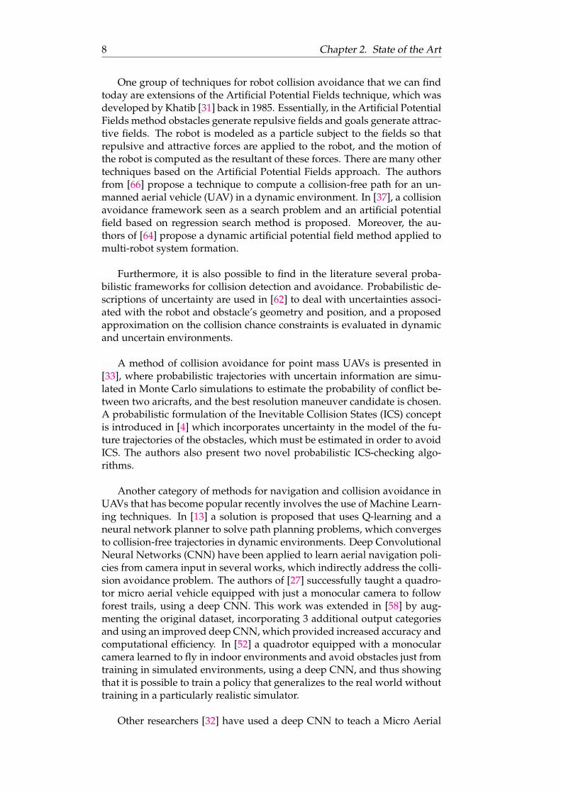
One group of techniques for robot collision avoidance that we can findtoday are extensions of the Artificial Potential Fields technique, which wasdeveloped by Khatib [31] back in 1985. Essentially, in the Artificial PotentialFields method obstacles generate repulsive fields and goals generate attrac-tive fields. The robot is modeled as a particle subject to the fields so thatrepulsive and attractive forces are applied to the robot, and the motion ofthe robot is computed as the resultant of these forces. There are many othertechniques based on the Artificial Potential Fields approach. The authorsfrom [66] propose a technique to compute a collision-free path for an un-manned aerial vehicle (UAV) in a dynamic environment. In [37], a collisionavoidance framework seen as a search problem and an artificial potentialfield based on regression search method is proposed. Moreover, the au-thors of [64] propose a dynamic artificial potential field method applied tomulti-robot system formation.

Furthermore, it is also possible to find in the literature several proba-bilistic frameworks for collision detection and avoidance. Probabilistic de-scriptions of uncertainty are used in [62] to deal with uncertainties associ-ated with the robot and obstacle’s geometry and position, and a proposedapproximation on the collision chance constraints is evaluated in dynamicand uncertain environments.

A method of collision avoidance for point mass UAVs is presented in[33], where probabilistic trajectories with uncertain information are simu-lated in Monte Carlo simulations to estimate the probability of conflict be-tween two aricrafts, and the best resolution maneuver candidate is chosen.A probabilistic formulation of the Inevitable Collision States (ICS) conceptis introduced in [4] which incorporates uncertainty in the model of the fu-ture trajectories of the obstacles, which must be estimated in order to avoidICS. The authors also present two novel probabilistic ICS-checking algo-rithms.

Another category of methods for navigation and collision avoidance inUAVs that has become popular recently involves the use of Machine Learn-ing techniques. In [13] a solution is proposed that uses Q-learning and aneural network planner to solve path planning problems, which convergesto collision-free trajectories in dynamic environments. Deep ConvolutionalNeural Networks (CNN) have been applied to learn aerial navigation poli-cies from camera input in several works, which indirectly address the colli-sion avoidance problem. The authors of [27] successfully taught a quadro-tor micro aerial vehicle equipped with just a monocular camera to followforest trails, using a deep CNN. This work was extended in [58] by aug-menting the original dataset, incorporating 3 additional output categoriesand using an improved deep CNN, which provided increased accuracy andcomputational efficiency. In [52] a quadrotor equipped with a monocularcamera learned to fly in indoor environments and avoid obstacles just fromtraining in simulated environments, using a deep CNN, and thus showingthat it is possible to train a policy that generalizes to the real world withouttraining in a particularly realistic simulator.

Other researchers [32] have used a deep CNN to teach a Micro Aerial

2.2. Social Drone Navigation 9

Vehicle a controller strategy that mimics an expert pilot choice of action sothat the quadcopter can autonomously navigate indoors and can find a spe-cific target. A similar work can be found in [65], where a simulated quad-copter successfully learns obstacle avoidance policies by training a DeepNeural Network with simulated raw sensor inputs. Finally the authors of[39] successfully taught an UAV to safely navigate in the streets of a cityby training a deep CNN with self-driving cars data. The CNN was able toaccurately predict steering angle as well as probability of collision, and thelearned policy generalized to indoor environments.

Other collision avoidance techniques that do not belong to previous cat-egories are [23, 12, 57]. In the first, the authors present a Mixed-IntegerLinear Programming method where the collision avoidance and path plan-ning task is formulated as a system of linear constraints with an objectivefunction that a software solver must solve. In [12], researchers employpartial order techniques to guarantee collision avoidance between vehi-cles advancing unidirectionally along a path. Other researchers [57] haveproposed a method for local obstacle avoidance by indoor mobile robotsthat formulates the problem as one of constrained optimization in velocityspace, where the robot chooses velocity commands that maximize an objec-tive function while satisfying all the constraints.

A completely different approach presented by Lee [36] is based on theassumption that large nervous systems are not necessary for accurate con-trol, and a tau-coupling technique is proposed to synchronize movementsand regulate their kinematics so that obstacles can be avoided. Finally, acollision avoidance technique in densely populated multi-agent environ-ments is presented in [38], consisting in an extension of the Velocity Obsta-cle concept, under the assumption that all agents make a similar collision-avoidance reasoning, resulting in safe and oscillation-free motions for eachof the agents.

In the present work we have taken the machine learning approach tothe collision avoidance problem. Inspired by the good results obtained in[21], a neural network has been trained with data from simulated collisions,so that the model learns to predict collisions. With this collision predictionswe built a simple trajectory correction mechanism that successfully avoidsthe imminent collision.

2.2.2 Human Motion Prediction

A fundamental requirement for an effective navigation is the ability to es-timate the future outcome of dynamic elements that are present in an en-vironment. In the case of Social Navigation it is assumed that a robot issharing the environment with people, therefore being able to estimate thefuture position of people has the potential of increasing the effectiveness ofthe navigation task. For this reason, Human Motion Prediction becomes abasic requirement in any serious implementation of Social Navigation, anda decent amount of research has been dedicated to this issue [35].


A great variety of methods can be found in the literature that tackle theHuman Motion Prediction task. In [5] it is assumed that people usuallyfollow specific trajectories or motion patterns corresponding to their inten-tions, and propose a technique, based on a hidden Markov model derivedusing the expectation maximization algorithm, for learning collections oftrajectories that characterize typical motion patterns of persons. However,this technique has the disadvantage of lacking flexibility on abnormal ob-servations. Other authors propose a clustering method and three differentprediction strategies based on the quality of the matching [9]. In [51], hu-man motion is inferred by a motion predictor using a stochastic processmodel to generate probability distribution maps of human existence. Otherresearchers [6, 41] have proposed the use of neural network architectures.All these techniques fall into the group known as place-dependent, becausethe predictive model must be learned for each of the environments whereHuman Motion Prediction (HMP) is used.

A different group of HMP techniques are those based on geometry, whichdo not necessarily need to learn the human motion intentionality for eachspecific environment. In [19], a geometric based HMP method is proposedfor human motion prediction that uses human motion intentionality in termsof goals. Prediction is done by identifying final destinations based on the in-stantaneous tangent angle in combination with a grid-based probability as-signment to all final destinations. Another geometrical approach proposedin [18] predicts future trajectories by minimizing the variance of curvatureof forecast paths.

Mixed approaches can also be found in the literature, such as the workin [67], where a reward function is used to generate the optimal paths to-wards a destination. This method can also be used as a modeling of routepreferences as well as for inferring destinations. Finally, the authors of [11]propose a vision-based prediction to infer intentionality, characterized asthe combination of obstacles and free space pixels under the field of viewof the person, with the aim of detecting unusual pedestrian trajectories.

Again, the present work introduces a module for HMP based on a neu-ral network which is trained on data composed of partial human paths thatare recorded from simulations.

11

Chapter 3

Aerial Social Navigation

The previous chapter provides an overview of the state of the art regardingthe fields of Human Drone Interaction and Social Drone Navigation. Thischapter focuses on the Social Drone Navigation topic and will describe inmore detail the main techniques that exist in the literature that are of specialinterest from the point of view of the current work.

3.1 Introduction

One of the fundamental and most important topics in the Mobile Roboticsfield is Robot Navigation. Mobile robots have the distinctive ability of mov-ing in real world environments with an often high degree of freedom. Ter-restrial robots’ movement is confined in principle to the 2D plane, whileaerial and submarine robots can move in the three dimensional space. Withall this freedom, it comes the need to plan the movement with a certain tem-poral horizon, and to consider all the elements in the environment that canconstrain the movement in some way. At the end, this process of planningthe movement subject to certain constraints turns out to be a challengingtask that has long been studied and for which there is still not a generalsolution.

Many fundamentally different approaches have been proposed, inspiredfrom a great diversity of knowledge domains, and in the scope of this workwe are going to focus on the Artificial Potential Fields based approaches.For a more detailed explanation about these different approaches head tosection 2.2. The following subsections present the general definition of theArtificial Potential Fields framework in order to provide the reader with thebasic knowledge to understand more recent research works in the field.

3.2 Artificial Potential Fields

The Artificial Potential Fields is a real-time obstacle avoidance approach formobile robots proposed by Khatib [31] back in 1985. The technique dealswith the collision avoidance task in a more reactive way compared to tradi-tional methods that are based on higher level planning, allowing real-timerobot operations in a complex environment.

In the APF approach the environment surrounding the robot is modeledas an artificial potential field that contains attractive and repulsive compo-nents, and the robot is modeled as a particle subject to the forces generated

12 Chapter 3. Aerial Social Navigation

by the field. In a typical navigation task, a robot moves towards a goalwhile avoiding obstacles, therefore, goals generate the attractive componentof the potential field and obstacles generate the repulsive component of thepotential field. All this results in attractive and repulsive forces applied tothe robot, and their contributions are added to give a final force that gov-erns the final robot movement.

The potential function is a function of the drone’s position, denoted asP, and is defined as the resultant of the all the attractive and repulsive fields:

Utotal(P) = Uatt(P) + Urep(P) (3.1)

Forces are related to the potential field through its gradient: the neg-ative gradient of the potential function defines an artificial force which isthe steepest descent direction for guiding the robot to its final goal. In theequation 3.1, the final potential as a function of the robot position is definedas the summation of its two components. It is also possible to express thefinal force applied to the robot as the summation of the repulsive and at-tractive contributions, where the attractive force is the negative gradient ofthe attractive potential and the repulsive force is the negative gradient ofthe repulsive potential.

Ftotal(P) = −∇Utotal(P) = −∇Uatt(P)−∇Urep(P) (3.2)

Ftotal(P) = Fatt(P) + Frep(P) (3.3)

In a real situation it is common to have more than one obstacle in theenvironment, therefore equation 3.3 takes the following more general form,where n is the number of obstacles.

Ftotal(P) = Fatt(P) +n∑i=1

Firep(P) (3.4)

Now let’s focus on how the attractive and repulsive forces are defined.

3.2.1 Attraction Force

The attractive potential exerted by the goal is defined as

Uatt(P) =1

2kapf (P−Pg)2 (3.5)

where kapf is a positive coefficient, P is the robot location and Pg is thegoal location, which is assumed to be constant, thus the potential is just afunction of the robot’s position. Finally, the attractive force is the negativegradient of the attractive potential

Fatt(P) = −∇Uatt(P) = −kapf (P−Pg) (3.6)

3.2. Artificial Potential Fields 13

FIGURE 3.1: Uncertainty zone: The Uncertainty zone is rep-resented as a cylindrical area with radius r and height h.

This picture is extracted from L. Garza [15].

In a three dimensional space, the force applied to the robot as a result ofhaving a goal that generates an attractive potential is expressed in separatedcomponents as

Fattx(P) = −kapf (x− xg)Fatty(P) = −kapf (y − yg)Fattz(P) = −kapf (z − zg)

(3.7)

where (x, y, z) is the position of the robot and (xg, yg, zg) is the position ofthe goal, both expressed in cartesian coordinates.

3.2.2 Repulsion Force

In the definition of attractive force it is only taken into account the objects’positions because most of the time the goals are far from the robot and ob-stacle avoidance task ends when the robot reaches the goal. But in the caseof repulsive forces, a more accurate representation of the force that con-siders an uncertainty zone around the obstacle is required, to account forpossible sensor error and define a safe margin around the obstacle as therobot must maintain a safe distance to the obstacles at all times. Therefore,a cylindrical uncertainty zone is defined inside which it is assumed the trueobstacle position lies. The cylinder has radius r and height h and ρ(P,Pob)is the distance from the robot to the nearest point of the obstacle’s uncer-tainty zone, which is defined as

ρ(P,Pob) =

{d− r

cosα 0 <‖ α ‖≤ arctan( h2r )

d− h2 sinα arctan( h2r ) <‖ α ‖< Π

2

(3.8)

where d is the distance from the robot to the center of the uncertainty zone.Figure 3.1 provides a graphical representation of the uncertainty zone. Therepulsive potential field can then be defined as

Urep(P) =

0 ρ(P,Pob) > ρ0

12η[

1ρ(P,Pob) −

1ρ0

]20 < ρ(P,Pob) ≤ ρ0

∞ ρ(P,Pob) ≤ 0

(3.9)


where η is a positive potential factor, Pob is the closest obstacle to the robotand ρ(P,Pob) is the distance from the robot to the nearest point of theobstacle’s uncertainty zone, ρ0 is a constant called scope of the repulsivepotential that represents the largest impact distance factor and has to begreater than 0. The object will not be able to affect the robot’s path if thedistance between the robot and the object is greater than ρ0.

As before, the repulsive force is the negative gradient of the repulsivepotential function, which now takes the form

Frep(P) = −∇Urep(P) (3.10)

Frep(P) =

0 ρ(P,Pob) > ρ0

η[

1ρ(P,Pob) −

1ρ0

][1

ρ(P,Pob)2

]∇ρ(P,Pob) 0 < ρ(P,Pob) ≤ ρ0

∞ ρ(P,Pob) ≤ 0

(3.11)

3.3 Social Force Model

The problem of modeling pedestrian behaviour was first encountered inthe 1950s, and at that time the proposed solutions involved the study of themacroscopic dynamics similar to gases or fluids. Later, there was a shift inthe research community to more microscopic descriptions in which pedes-trian motion is described more as an individual particle rather than a whole.

In 1995, Dirk Helbing [30] presented a model in which the motion ofpedestrians is described by social forces that reflect the internal motiva-tions of the individuals to perform certain actions. The model defines aforce that makes the pedestrian maintain a desired velocity, another forcethat makes the pedestrian keep a certain distance to other pedestrians andborders, and a third force modeling attractive effects. The work providesevidence that the proposed social force model is capable of describing theself-organization of several observed collective effects of pedestrian behav-ior very realistically.

The results provided in [30] have remarkably good implications becausethey show that it is possible, and in principle straightforward, to integratethe modeling of pedestrian behaviour into the Artificial Potential Fieldsframework, as both Artificial Potential Fields and Social Force Model (SFM)represent interactions using forces. In fact, there is a very recent work [25] inwhich the Social Force Model is successfully extended to allow autonomousflying robots to accompany humans in urban environments in a safe andcomfortable manner. The extended approach, which is called Aerial SocialForce Model, introduces a module to estimate the destination of the per-son the drone is walking with. It also introduces a new metric to fine-tunethe parameters of the force model, and to evaluate the performance of the

3.4. Aerial Social Force Model 15

aerial robot companion based on comfort and distance between the robotand humans.

The model presented in this thesis is based on the Artificial PotentialFields object avoidance framework, in the sense that interactions betweenelements in the environment are modeled as forces. However, most of theinspiration of the present work comes from [25], because in that work theauthors propose a solution for the exact same problem we are interested insolving. Even though their proposed solution is different, it sill deserves adetailed explanation, which is provided in the following section.

3.4 Aerial Social Force Model

The development of the Aerial Social Force Model (ASFM) approach wasmotivated by the recent advances in aerial robot technologies as well asthe fact that the research on robot companion was relatively minimal atthat time, and still it is. Due to the lack of previous research in the field,the researchers had more freedom regarding system design and ended upproposing a new robot companion approach that is a 3D extension of theSocial Force Model (SFM) introduced by Helbing [30].

The main difference of ASFM with regard to the original SFM work isthat in the extended approach the interest is not to model the motion ofpedestrians. The goal in ASFM is to apply the defined interaction forcesto the aerial robot so that it behaves like another pedestrian. And since anUAV can fly in the three directions of space, ASFM also extends the originalmodel to three dimensions so that the drone can fly at different altitudes ina human-like way.

The ASFM can be described as three separate modules: 1) the regres-sion model used to estimate people’s motion, 2) the interactive forces of theaerial force model, and 3) the quantitative metric used to evaluate the per-formance of the robot. All these modules are described in more detail in thefollowing subsections.

3.4.1 Online Regression Model for Human Path Prediction

One of the goals of ASFM is to allow a drone to navigate side-by-side witha human. This is actually not a trivial task because it requires the model tomake an estimate about the path that the human is following and anticipatethe future position of the human. Otherwise, the drone would tend to flyslightly behind the human because it would be reacting to the present hu-man position without any kind of anticipation.

The proposed solution to this problem consists of integrating an onlinelinear regression model which takes a sequence of observed past humanpositions and predicts the future position. The linear regression model isdefined as


f(X) = w0 +

p∑j=1

Xjwj (3.12)

where the p is the number of past positions considered, the input vectoris defined as X = (∆x1,∆x2, ...,∆xp) and w = (w1, w2, ..., wp) are the un-known parameters of the model that must be adjusted during the learningprocess. Notice that the human positions are expressed as increments in-stead of globally. This way of expressing the position is very common inMachine Learning applications because it ensures that all the inputs comefrom the same distribution.

To estimate the optimal values for the model’s parameters, X and Ymatrices are built. The matrix X contains all the input samples on whichthe model is going to be trained, while the Y matrix contains the targetsthat the model must learn to predict, and the number of samples N is 100.An input sample contains the past 5 human position increments, p = 5,and it corresponds to a row in the X matrix. Therefore, X has dimensions(N−p)x(p+1). The target associated to each sample contains the next incre-ment in position with respect to the sequence of increments in the sample,and corresponds to a row in the Y matrix. Therefore, the Y matrix hasdimensions (N − p)x1.

X =

1 ∆xn1,1 ∆xn2,2 · · · ∆xnp,p

1 ∆xn2,1 ∆xn3,2 · · · ∆xnp+1,p...

......

. . ....

1 ∆xnN−p,1 ∆xnN−p+1,2 · · · ∆xnN−1,p

(3.13)

Y =[∆xp+1,∆xp+2, ...,∆xN

]T (3.14)

With the previous two matrices, which are built from collected dataabout pedestrian paths, the model’s parameters are optimized using thewell-known optimization method Gradient Descent. The cost function thatthe optimizer has to minimize is defined as follows.

J(w) =

N∑i=1

(f(X)− y)2 (3.15)

The optimization process is iterative, and in each iteration the gradientof the cost function with respect to each weight is computed and used toupdate each weight so that the value of the cost function in the next iterationis smaller. The iterative process continues until the value of the weightsconverge to the minimum. In each iteration the cost function is evaluatedfor all the samples in the dataset, and then its gradient is computed withrespect to each weight as

∆J(w) =

(∂J

∂w0,∂J

∂w1, ...,

∂J

∂wp

)(3.16)


∂J

∂wp=

1

N − p

N−p∑i=1

p∑j=0

Xijwj − yi

Xp (3.17)

Once the gradient is known, it is important to decide how much to movein the gradient direction, which has a significant impact to the performanceof the optimization process. If the step is too short, convergence will be veryslow. On the other hand, if the step is too large, it is possible to jump theminimum and end in a place of the weight space where the cost is higherand thus convergence can not be achieved.

In ASFM, the strategy used to move throught the gradient is the RM-Sprop method, proposed by Geoff Hinton in an unpublished work. Themethod states that dividing the gradient by the root of the expected valueof the gradient, taking into account a short window, makes the learningwork much better. The weights are updated as

wt+1 = wt −η√

E[∇J(w)2]t + ε∇J(w) (3.18)

E[∇J(w)2]t = γE[∇J(w)2]t−1 + (1− γ)∇J(w)2t (3.19)

where E[∇J(w)2]t means the decaying average over past squared gradi-ents, γ means the momentum value, typically set to 0.9 or 0.95, and always< 1, and ε is a smoothing term that avoids the division by zero value.

Once the linear regression model is trained using Gradient Descent withRMSprop, the resulting model is able to make predictions about the posi-tion of the human in the next time interval given a sequence of the last 5positions. This result is then used in the next module to allow the drone tonavigate side-by-side with the human.

3.4.2 Interactive forces definition

In the Social Force Model it is claimed that changes in behavior (trajectory)can be explained in terms of social fields or forces, and the final motioncan be expressed through a function of the pedestrians’ positions and ve-locities. The ASFM is based on these assumptions and introduces a flyingrobot in the social environment, taking into account the interaction amongthe robot, people and obstacles.

The total force applied to the robot comes from three separate compo-nents: the robot-humans and robot-objects interaction forces, as well as theattraction forces, which make the robot stay closer to the human being ac-companied

FR = fgoalR + FintR (3.20)


where FintR is defined as the summation of all the repulsive forces exerted

by other pedestrians and objects, defined as

FintR =

∑pj∈P

f intRj +∑o∈O

f intRo (3.21)

where P is the set of people moving in the environment and O is the setof obstacles. Next, each interaction force affecting the robot individually isdefined.

3.4.3 Goal attraction force

The objective of this force is to drive the robot to the goal, which means tostay next to the companion. The force is defined as the summation of twoindividual attractive forces, one which pursues the position of the humanbeing accompanied, and the second one that pushes the robot to the humanforecasted position in the next future step. Both forces are defined as

fgoalR = k(v0R − vR) (3.22)

where vR is the robot’s current velocity. v0R = v0

ReR means that therobot tries to move at a desired speed v0

R in a desired direction eR, and thisdesired direction actually points to the goal. Thus, the result of this forcewill be to move the robot towards the goal at a constant desired speed.

3.4.4 Robot-object interaction force

The drone must keep a certain distance from objects when navigating, inorder to avoid collisions so that the drone can reach its goal. Therefore,it is necessary to consider the objects around the robot, which will exertrepulsive forces on the drone defined as

f intRo = −∇rRoURo(||rRo||) (3.23)

URo(||rRo||) = U0Roe

−||rRo||c (3.24)

where the vector rRo is defined as the difference between the location ofthe robot and the location of the obstacle o that is nearest to the robot. Theterm c is a parameter of the model that governs the slope of the repulsionmodule. Notice that the module of the repulsive force URo(||rRo||) is a non-linear function of the distance. As a result, the repulsion will only be sig-nificant when the distance of the robot to the object is small, otherwise therepulsion will be negligible.

3.4.5 Robot-human interaction force

Pedestrians, similarly to objects, exert a repulsive force over the drone be-cause they are potential obstacles. However, pedestrians are human beingsthat move freely in the environment, and similar to the drone, they try tokeep a certain distance to obstacles as well as the drone itself. Additionally,


humans have a personal space around them that defines a volume, and thepresence of undesired external objects inside this volume causes discom-fort. Therefore, to model the repulsion exerted by humans onto the drone,a more complex definition that considers personal space is required.

The repulsive force exerted by a human onto the robot is defined as

f intRj = ARje

(dR−dRj

BRj

)rRj(t)

dRj(t)ψ(ϕRj , θRj) (3.25)

where ARj , BRj and dR are some of the parameters that must be learned inorder to fine tune the ASFM. The term ψ(ϕRj , θRj) is defined as

ψ(ϕRj , θRj) = ω(ϕRj)cos(θRj)(h+ ξRjω(ϕRj)) (3.26)

and represents the anisotropic factor of the human in a 3D space. The termappears multiplying the rest of the expression, thus its value has a directimpact on the magnitude of the repulsive force. The anisotropic factor de-pends on ϕRj , an angle formed between the desired velocity of the pedes-trian pj and the vector rRj (which is the distance between the robot andthe pedestrian pj and pointing to him) and θRj , which is the angle betweenthe x and z coordinates, an angle formed between the position of the robotand the pedestrian. The constant h is the height of the pedestrian. Finally,ω(ϕRj) is defined as

ω(ϕRj) = λRj + (1− λRj)(

1 + cos(ϕRj)

2

)(3.27)

where λRj defines the strength of the anisotropic factor and is the remainingparameter that must be learned. Lastly, cos(ϕRj) is computed as

cos(ϕRj) = −nRj · epj (3.28)

Here, nRj is the normalized vector pointing from the robot to pj andrepresents the direction of the force, and epj is the desired motion directionof the pedestrian pj .

The drone has also an anisotropic factor in 3D, which is taken into ac-count when computing the repulsive force exerted by the drone onto thehuman. However, as the drone is in the air all the time, the anisotropic fac-tor is symmetric and its expression is simpler, as shown in equation 3.29.Figure 3.2 includes several plots that show the shape of the anisotropic fac-tors for the human and the drone.

ψ(ϕRj , θRj) = ω(ϕRj)cos(θRj) (3.29)

Finally, we can define the total force that will drive the aerial robot asthe summation of all the previously defined interaction forces:

FR = fgoalR,dest + fgoalR,i + FintRj + Fint

Ro (3.30)


(A) (B) (C) (D)

(E) (F) (G) (H)

FIGURE 3.2: 3D view of the anisotropic factor. The toprow shows the human’s anisotropic factor when the param-eters λRj = 0.25 and ξRj = 0.25. The bottom row shows theanisotropic factor for the drone, when λRj = 0.9 in (E) and

(F) and when ξRj = 0.5 in (G) and (H)

One last important thing to mention is that the ASFM implements amechanism to limit the maximum velocity of the drone depending on itsproximity to a human, for safety reasons. The model defines three zonesinspired on how people interact:

vR =

vsafety

dRj

ω(ϕRj) ≤ µsafetyvcruise µsafety <

dRj

ω(ϕRj) ≤ µsocialvfree otherwise

(3.31)

3.4.6 Quantitative Metrics

The last component of the Aerial Social Force Model that deserves a sepa-rate description is the quantitative metric that is used to evaluate the perfor-mance of the task accomplished by the flying robot. The presented metric istotally new and is based on proxemics, proposed by [28]. The work defines 4distances between people: (1) intimate distance (0-45cm); (2) personal dis-tance (45cm-1.22m); (3) social distance (1.22m-3m); and (4) public distance(> 3m).

The ASFM borrows the distances proposed in [28] and defines threevolumes centered at the human’s position as follows.


A = {x ∈ R3\(B ∪pj C)|d(x, pi) < 3}B = {x ∈ R3\C|d(x, pi) < 3ψ(ϕpi , θpi)}C = {x ∈ R3|d(x, pi) < ψ(ϕpi , θpi)}

(3.32)

The volume C represents the human’s personal space, and the robotmust not enter this region. B is the region where the robot sould ideallybe as it represents the human’s field of view, and the drone should be atsight all the time for a correct interaction. Region A is the social space. Therobot can be in this region but it is preferred that the robot is closer to thehuman, in region B.

By representing the robot as ψ(ϕRj , θRj), it is now possible to define anexpression for the performance of the task accomplished by the robot interms of the overlapping volumes. The perfromance metric is defined as:

ρ(r, pi) =

∫(B\∪pjCj)∩R

dx

|R|+

∫(A\∪pjCj)∩R

dx

2|R|∈ [0, 1] (3.33)

The range of the performance metric is defined between 0 and 1 andhas the following interpretation. If the complete area of the robot is allo-cated in zone B, the performance gets the maximum value, i.e., 1. As therobot moves far from the person and enters to zone A, the performance de-creases down to 0.5, when all the volume of the drone is inside region A.If the drone keeps moving far from the person, the performance measurewill decrease down to 0, when the volume of the drone is no longer inter-secting with neither region B or A. Finally, if the volume of the drone istotally contained in region B initially, and it moves closer to the human, theperformance will decrease from 1 down to 0, when all the drone’s volumeis inside region C.

Here ends the detailed explanation of the Aerial Social Force Model ap-proach, on which the work presented in this thesis is based. Next chapterbegins the detailed description of the Neural Aerial Social Force Model byfirst explaining in the process of generating the data as well as the featuredefinition that was found to provide the best results.

23

Chapter 4

Data Generation and FeatureDefinition

Regarding motion control of the drone, the data dependency of the pro-posed technique only involves the final step of learning a function of theinteraction forces that maps to a resulting force applied to the drone, orequivalently an acceleration applied to the drone. However, the impactthat this learned function has on the resulting motion of the drone is huge.Therefore, most of the effort dedicated to the development of Neural AerialSocial Force Model (NASFM) has been directed to the tasks of generatingthe dataset and training the models so that they learn useful motion con-trol policies. This chapter is going to center the attention on the procedurethat has been followed to generate an adequate dataset, which involves thesubtasks of generating the expert trajectories and defining useful features.

4.1 Expert Trajectories Generation

NASFM is formulated under the assumption that it is possible to learn amodel that generates a flying behaviour that mimics that of a drone teleop-erated by a human expert, provided that there is enough data about the ex-pert’s policy and the model used to learn the function is expressive enough.Thus, the first step is to gather data about the expert’s policy. To do so, sim-ulated environments have been used because they are safe, easy to run andallow complete freedom of environment design, compared to gathering thedata from a real drone. Using a PS3 controller the human expert is able tomove the drone in the simulated environment and all the necessary data isrecorded and stored.

It is important to note that sometimes it is not feasible to train a modelon simulated data because there is no guarantee that the trained model cangeneralize to real data. This problem arises if the data from the simulatedenvironment and the real data come from different distributions, which canhappen in some situations. In our case, this is not an issue because our datais composed of forces, which are functions of the distance from the droneto the different objects in the environment, so the distributions of data fromthe simulated environment and the real world are expected to be very sim-ilar.

24 Chapter 4. Data Generation and Feature Definition

Environment type train validate testAB yes yes yesD yes yes yes

KL yes yes yesM no no yesC no no yes

Lab yes yes yesCollisions yes yes yes

TABLE 4.1: Summary of all the environments used in thedevelopment of the present work.

4.1.1 Training, Validating and Testing the models

Before introducing the simulator and describing the simulated environ-ments, it is important to make clear the difference between training, val-idating and testing the models. To train, validate and test a model, thedataset that contains the expert trajectories is split into three different por-tions of different size, where the train set is typically about four times biggerthan validation and test sets. Training a model means running an algorithmthat automatically optimizes the parameters of the model by learning pat-terns in the training set, so that the training accuracy is increased over time.Validating a model is the process of evaluating the learned model on un-seen data and using the result of the evaluation to tune the hyperparame-ters of the model so that they are better adapted to learn. Finally, testinga model means providing a final score indicating the performance of thetrained model.

In the context of this work, the generated datasets, which are made fromthe provided expert trajectories for a given type of environment, are splitinto train, validation and test sets. The models that do not have hyperpa-rameters are trained on the training set and then tested on the test set. Themodels that do have hyperparameters are trained on the train set and thenthe validation set is used to adjust the hyperparameters. The final perfor-mance is obtained by testing the models on the test set. Additionally, tomeasure the performance of the policy learned by a model, it is simulatedon the test environments, which means that the trained model is used tocompute the control actions that move the drone in real time.

During the development of the presented work, a total of 7 differenttype of environments were generated with different goals in mind. Fromthese, a subset of 6 environment types were entirely dedicated to the task oflearning a control policy from expert demonstrations, as described in 4.1.4to 4.1.8. The remaining type of environment was used to simulate collisionto build a dataset to train the collision detection model, as presented insection 5.2.1. Table 4.1 summarizes all the environments used and theirroles during the development of the presented work.

4.1. Expert Trajectories Generation 25

4.1.2 The simulator

The software that was used to build and run the simulator is FreeGLUT[1]. FreeGLUT is an open-source alternative to the OpenGL Utility Toolkit(GLUT) library, which has been used in a wide variety of practical appli-cations because it is simple, widely available and highly portable. It takescare of all the system-specific chores required for creating windows, ini-tializing OpenGL contexts, and handling input events, so it provides allthe features that our simulator requires. The Gazebo simulator is actuallya better option as it provides all the features that this project requires, itincludes physic engines, it integrates easily to ROS projects and there is apackage that simulates the actual ARdrone. However, at the end FreeG-LUT was chosen because most of the work of building the simulator andenvironments had already been done by another student that was work-ing with the Extended Social Force Model applied to terrestrial robots, andthus all the additional adaptations that were done for this thesis involvedextending the simulator from a two-dimensional representation to a threedimensional representation. Building the simulator in Gazebo from scratchwould have required much more effort, and this was out of the scope of thethesis.

The simulator is built in such a way that it generates a simulated en-vironment, which must be defined following a strict format in a text file,and which is specified when the simulator is launched. During the simu-lation an output text file is generated each time the simulation is updated,which happens at a frequency of 30Hz. The directory where the output ofthe simulator is stored must be specified when it is launched. The simula-tion ends when the condition that ends the simulation (explained below) ismet. Thus, the information generated by a single run of the simulator fora given environment is a directory with as much output files as simulatediterations. Each output file contains the position of all the objects in the en-vironment so that it is possible to compute any distance between any pairof objects, and consequently any interaction force.

4.1.3 The simulated environments

During the development of this work, 6 different types of environmentshave been defined and simulated, each kind containing different elements,but there are three objects that are found in all environments: the drone, thecompanion and the goal. The drone appears in all environments becauseis the object that the human expert is teleoperating with a PS3 controller.Additional information about this object is written in the output files: itsposition, velocity and acceleration. The companion appears in all environ-ments because it is the object that the drone must follow. Its movementis autonomous and is governed by the Artificial Potential Fields technique.Finally, the goal is the object that takes the role of goal in the APF model im-plemented in the companion, thus the companion allways moves towardsthe goal, and all simulations end when the companion reaches the goal.

There are four other objects that appear on some of the environments:walls, trunks, canopies and bots. Walls are rectangular objects that can take


any desired dimensions and represent obstacles like walls or beams. Trunksare cylinders defined by a height and radius and are used to represent thetrunk of a tree or a column. Canopies are spherical objects that only repre-sent the canopy of a tree. Finally, bots are moving obstacles that representpedestrians. Each bot’s movement is governed by the APF method and itsgoal is specified in the environment definition file. Unlike the companion,when a bot reaches its goal it defines a new goal that is its position at thebeginning of the simulation, and when it reaches this new goal, the nextgoal becomes the initial goal, and it continues this way in an endless loop.

The following subsections describe each one of the 6 kind of environ-ment that have been used in the main task of learning a flying control policyfrom demonstrations. Some environment types are only used for training,others are only used for testing and a few others are used for both trainingand testing.

4.1.4 Open space without static obstacles and bots (AB)

The first type of environments that were simulated are the simplest possi-ble. They only contain the drone, the companion and several consecutivegoals. They are labeled as type A and type B because there are two dis-tinctive environment definitions that have slight differences although theelements that appear in both are the same. This is the reason why theyare grouped into one category. Type A environment have 5 consecutivegoals that are close to one another and define a random path. Type B en-vironment have only 3 goals, randomly placed in the same way. The maindifference between the two types is the drone’s initial position. In type Aenvironment the drone always appears near the companion at a height thatis typically maintained throughout the simulation, while in type B environ-ment the initial position of the drone is much more variable in height anddistance, and thus the human expert must initially move the drone close tothe companion. Type A and B environments were used to teach the modelsthe easiest possible policy. A total of 80 expert trajectories for type A and80 expert trajectories for type B environments were recorded, the first 62 ofeach kind were dedicated to train the models (124 in total), the next 8 ofeach kind were used to validate the models and the remaining 20 trajecto-ries were used for testing the performance of the learned policies.

Type B environments exist because initially the models were trainedonly in type A, and due to the initial configuration of the drone, they weren’table to learn correct height control policies, as no demonstrations were pro-vided in the expert trajectories. A picture of a type B environment can beseen in figure 4.1.

4.1.5 Open space with bots and without static obstacles (D)

The following type of environment that was simulated introduced bots, andis identified as type D. Here, the companion has a sequence of 5 consecutivegoals that he must reach, as in type A environments, and the initial positionof the drone is randomly defined significantly far from the companion, as intype B environments. Additionally, there are bots moving randomly in the


FIGURE 4.1: Cropped screenshot from the simulator viewfor a type B environment. The visible elements are: thecompanion (green legoman), the drone and the goal (greencylinder). The red circle on the floor is the predicted com-

panion position one second into the future.

FIGURE 4.2: Cropped screenshot from the simulator viewfor a type D environment. The visible elements are: thecompanion, the drone, the current goal and the bots (red

legomen).

open space that must be avoided by the companion and the drone. A totalof 80 different environments were simulated, 65 of which were dedicated totrain the models and the remaining 15 to validate the models’ accuracy andtest the performance of the learned policies. A screenshot of the simulatorview can be seen in figure 4.2.

4.1.6 Open space with static obstacles and without bots (KL)

The next category of simulated environments contains two types of envi-ronments: type K and type L. The common thing about the two is that theyonly contain static obstacles, apart from the drone, the companion and asingle goal. Type K environments only contain a column (a trunk obstacle)that is placed between the starting companion position and the goal, with a


FIGURE 4.3: Cropped screenshots from the simulator viewfor a type K (left) and type L (right) environments. Left: thevisible elements are the drone, the companion, the goal andthe column. Right: the visible elements are the drone, thecompanion, the bridge on the front and the column on the

back. The goal is occluded by the column.

slight displacement to a randomly chosen side, so that sometimes the com-panion will circle the obstacle on the right and other times it will circle theobstacle on the left side. Type L environments are an extension of the Ktype as they include a bridge structure positioned in front of the column.The bridge structure is composed of two separated columns and a wall thatis shaped as a beam joining the two columns at a certain height. The ideaof including the bridge is to force the drone to avoid obstacles that do notblock the companion and must be dodged by passing below or above. Acropped screenshot from the simulator view for type K and L environmentscan be seen in 4.3.

Expert trajectories were recorded for 100 environments type K, of which80 were used to train the models and the rest to validate them. In the caseof environments of type L, 130 different environments were simulated, ofwhich 105 were used for training and the remaining were used to validatethe models. It is important to note that this category of environments wasonly used to teach the models the expert policy, but the performance of thelearned policy was not measured on this category of environments, andinstead, it was measured on environments with more obstacles similar tothose found in this category. The validation set is always necessary becausewe need some way to check that the models are learning properly, and wecan only do so by measuring their accuracy on unseen data.

4.1.7 Test environment with static obstacles and without bots (M)

The last two categories of simulated environments are different from therest in the sense that they have only been used to test the policies that weretrained in the KL type environments. The first type of test environmentsare identified as M and only contain the drone, the companion, one goalper environment and static obstacles. The static obstacles are columns andbridges and their numbers are random but always greater than one. There-fore, they can be considered as a more complex version of the KL type. Atotal of 20 M-type environments were generated just for testing purposes.A frame from the simulator’s view window is shown in figure 4.4


FIGURE 4.4: Frame from the simulator’s view for a type Menvironment. The visible elements are: the companion, thedrone and several columns and bridges. The goal is out of

vision in the direction the companion is heading to.

4.1.8 Test environment with static obstacles and bots (C)

Finally, for the last category of test environments, we included all the el-ements available in the simulator to built the most complex type of envi-ronment, identified as C. This kind of environment includes the drone, thecompanion, one goal per environment, canopies, trunks and bots. Bridgesand columns do not appear and instead there are trees which are composedof a trunk and a canopy with variable dimensions. Between 4 and 6 botspopulate the environment and move towards their respective goals, accord-ing to the mechanism described in section 4.1.5.

A total of 70 environments of this kind were generated, but only the first20 were used to test the learned policies. Initially, this type of environmentswere used to train the models. However, it was not possible for the mod-els to learn any useful policy and thus they were later used to test modelstrained in the more simple KL environments. A frame from the simulator’sview window is shown in figure 4.5

4.1.9 Space replicating laboratory conditions (Lab)

The need to generate simulated environments that replicate the conditionsof the laboratory where the real drone is tested appeared when we testedthe learned policies in the gazebo simulator. The behaviour of the drone onthe gazebo simulator, which replicates the conditions found in the lab dur-ing real experiments, was unsatisfactory. Two main reasons were identifiedthat could explain such result: (1) the model was trained on unconstrainedspaces, while the available space in the laboratory is limited to a volume ofless than 5x5x2.5m; and (2) the model was trained on environments wherethe companion is constantly moving. Note that the two conditions are ac-tually related, because in a small space the companion is expected to standstill most of the time. At the end, the issue can be summarized to "trainingconditions don’t match test conditions", which is the same as saying "the


FIGURE 4.5: Frame from the simulator’s view for a type Cenvironment. The visible elements are: the companion, thedrone, the bots and several trees. The goal is occluded by

the trees in the background.

distribution of the data used to train the model does not resemble the dis-tribution of the data used to test the model". After realizing that the learnedpolicies would not work properly in real experiments, we were forced togenerate a new type of environment, which was labeled as Lab type.

Lab type environments are similar to type K in the number of elementspresent, they contain the drone, the companion, a sequence of 6 goals andan obstacle, which is thinner. The main difference is that in Lab environ-ments the available space is significantly reduced and the behaviour of thecompanion is different. When the companion reaches a goal, it stays a ran-dom amount of time still, before moving towards the following goal. Thisnew behaviour produces a companion behaviour more similar to that ex-pected in the real experiments. Furthermore, the human that controls thedrone must stop the drone next to the companion while he is not moving.Another difference with the previous environments is that the goals arenow hidden to the human expert, in order to avoid the tendency to movethe drone towards the goal instead of blindly accompanying the compan-ion. Figure 4.6 provides a screenshot of the simulator view for this kind ofenvironment.

4.1.10 Technical details about environment generation

After reading about the previous three categories of environments, onewould expect one more last category to contain static obstacles and bots.However, this is not the case because the policies learned from environ-ments of types K and L generalize to the case where static obstacles andbots are present. The reason for this is that the drone learns to follow thecompanion at a height in which pedestrian are no longer obstacles to beavoided, and thus the problem of avoiding people is solved. But, there is asituation in which this method would not work. In case there are obstaclesat the height of the drone, they would force the drone to lower its height

4.2. Feature Definition 31

FIGURE 4.6: Cropped screenshots from the simulator viewfor two different type Lab environments. The availablespace is significantly reduced, goals are hidden and the ob-stacle is shaped like the obstacles found in the laboratory.

so that it enters the space where pedestrians can be found. However, thissituation is out of the scope of this work due to its complexity, and thereforethe mentioned simplification is valid.

Another important thing to mention is that for a given type of environ-ment it is necessary to generate environments that contain the same ele-ments but have some kind of variability on different aspects. The orienta-tion of the world must be different, the position of obstacles, goals, bots,and companion must be different, the relative position of the drone to thecompanion at the beginning of the simulation must be different, etc. Allthis variability ensures that the models will not overfit to certain motionpatterns that should not be learned, as well as making the models morerobust and invariable to rotations. This is also necessary if we want ourlearned policies to generalize to unseen environments.

4.2 Feature Definition

As it has been said in the introduction of the chapter, the task of building adataset from scratch can be divided into two steps: (1) obtain data about theproblem, and (2) extract useful information from the data that will be usedto train the models, which involves the extraction of previously definedfeatures. The first step of obtaining the raw data has been explained in theprevious section. In this section, we are going to discuss the chosen featuredefinition. The defined features will allow us to extract useful informationfrom the raw data, which is composed by the output from the simulatedexpert trajectories. These extracted features can then be put together into adataset from which the learning algorithms will be able to learn useful mo-tion control policies. Thus, the dataset will be composed of samples, onefor each frame of simulation, and each sample will contain several features.

One important issue to mention is that in this work the task of learninga motion control policy for a flying robot based on the Aerial Social ForceModel is addressed for the first time. This means that there is no avail-able information in the literature about the best definition of features. As aresult, the feature definitions proposed in this work are influenced by theoriginal Aerial Social Force Model although some modifications have been


included because experimental evidence proves their improvement on theoverall system performance.

4.2.1 Companion Attractive Force

The policy that we want our models to learn is one that makes the drone ac-company a person, which means flying side by side with the human whilekeeping a safe distance. Therefore, the models need some kind of infor-mation that represents the relative position of the drone to the companion,and this is why the companion attractive force feature is used. The featureis defined as follows

fc = Pc −PR (4.1)

where Pc is the current position of the companion and PR is the current po-sition of the drone. This feature is actually not a force because it is definedas just the vector difference of the companion position and the drone posi-tion. In the original ASFM the interaction force between the human and thegoal is a function of the velocity and so it is a real force. In the context ofthe Neural Aerial Social Force Model, however, it is defined as a functionof the difference in position due to empirical evidence: the tested policiesbehave smoother and have less overshoot when the companion attractiveforce is defined as a function of the position instead of velocity.

4.2.2 Goal Attractive Force

In order to have a flying behaviour in which the drone is not following thecompanion from behind and instead is moving side by side or even slightlyadvanced to the human, the drone needs some notion of the path the hu-man is following, and this can be done by predicting the human’s futureposition in the near future. This is the reason why the proposed systemintegrates a module for human path prediction, which is used to computethe goal attractive force feature.

This feature follows the same definition as the companion attractiveforce feature but instead of computing the difference in position betweenthe companion and the drone, it computes the difference in position be-tween the drone and the predicted future companion position as follows

fg = Pg −PR (4.2)

where Pg is estimated for one second into the future. Figure 4.7 show therepresentation of companion and goal attractive force features.

4.2.3 Static Object Repulsive Force

A fundamental ability for any mobile robot is to effectively avoid obstacles,as not being able to do so could potentially cause damage to the robot oreven destroy it. Therefore, the robot needs some information about the rel-ative position of obstacles in order to plan its movement in such a way thatthey are avoided. In the APF framework this information is encoded into

4.2. Feature Definition 33

FIGURE 4.7: Representation of companion and goal attrac-tive force features. FALTA DIBUIXAR ELS FEATURES.

the object repulsive force, which aggregates all the individual object inter-action forces into one. Due to its proven effectiveness, we have includedthis force without any changes to our set of features. The definition of theobject repulsive force feature is:

Fo =O∑o=1

fo (4.3)

where O is the set of detected objects and fo is defined as,

fo =Po −PR

‖Po −PR‖AR,oe

(dRo−dR,o

BR,o)

(4.4)

where Po and PR are the positions of the object and the drone respectivelyand define the direction of the force, while AR,o, BR,o and dR,o are fixed pa-rameters that govern the module of the resulting force.

As it can be seen, the object repulsive force is a non-linear function of therelative positions of the obstacles with respect to the drone. Thus, the indi-vidual contributions to the final resulting force are non-linear, which meansthat the individual repulsive force of an object that is far from the drone willbe negligible compared to the individual repulsive force of an object that isclose to the drone. This effect is actually desired because when all repulsiveforces are added into a single resulting force, all the information is mixed,and we would like the repulsive force to maintain as much as possible thedirection of the closest obstacle. This effect can be adjusted by tuning theparameters AR,o, BR,o and dR,o.

4.2.4 Pedestrian Repulsive Force

Pedestrians can be considered as moving obstacles. However, unlike staticobstacles, pedestrians are humans, and humans have personal space, whichis a volume surrounding the human. Intrusions into the personal space of ahuman by external objects may cause discomfort to the human, especially if


the object is a flying robot. As a result, interactions with pedestrian must beconsidered separately from static objects. This is the reason why we havedefined another feature that provides information about the repulsion thatpedestrians exert over the drone, even though the definition is the same asin static obstacles,

Fh =H∑h=1

fh (4.5)

where H is the set of detected pedestrians and fh is defined as

fh =Ph −PR

‖Ph −PR‖AR,he

(dRh

−dR,h

BR,h)

(4.6)

where Ph and PR are the positions of the object and the drone respectivelyand define the direction of the force, while AR,h, BR,h and dR,h are fixedparameters that govern the module of the resulting force. By defining theinteractive forces of pedestrians in a separate feature it is possible to adjustthe module with the fixed parameters so that the repulsion is more intensedue to the additional personal space.

4.2.5 Drone Velocity Feature

The last feature that is extracted from the expert trajectories when build-ing the dataset to train the models is the current drone velocity vR. Thisfeature has nothing to do with forces or interactions between objects in theenvironment. Instead, it just provides information about the internal stateof the drone, which turns out to be crucial for the resulting policy to behaveadequately.

During the design phase of the features, it was observed that includingthe velocity of the drone as a feature allowed any model to learn decentpolicies, something that was not possible without including the feature.A possible intuitive explanation to this is that the control actions that thedrone must take, which are expressed as accelerations, depend on the in-stantaneous interaction forces with other objects in the environment as wellas the drone’s movement state at that moment in time.

As an example, imagine the drone is close to an obstacle and movingwith a velocity v1 > 0 perpendicular to the repulsive force exerted by thatobstacle. Now imagine that the drone is in the same position with a veloc-ity v2 > 0 and directed to the obstacle. If only the interaction forces areconsidered, these two situations would be represented by the exact samefeature vector. However, the expected action that the drone should take ineach situation is very different. In the first situation the drone is passingnear an obstacle without risk of collision, but in the second situation thedrone is about to collide if no collision avoidance maneuver is performed.Therefore, as this simple example illustrates, the velocity of the drone isvery relevant in order to choose the correct motion action, and this is thereason why it has been included as another feature in the dataset.

35

Chapter 5

Additional Requirements

The two previous chapters focus on the development of the motion con-troller for the drone, which involves generating expert trajectories, build-ing a dataset by extracting the defined features, and training the modelsthat will provide the control signals. With all this, the process of choosingthe correct control action for the drone given the state of the environmentis completely covered. In this chapter, the focus of attention is on the twomodules that have been mentioned but are still not explained in detail: thehuman path prediction module and the collision detection module.

5.1 Human Path Prediction

The Aerial Social Force Model approach includes a linear regression modelthat predicts future human’s positions based on the last 5 observed posi-tions, as explained in Section 3.4.1. The presented work also includes amodule for predicting future human positions based on Machine Learningtechniques, as it is a fundamental requirement in order to allow the drone towalk side-by-side with the human. However, the present human path pre-diction module is believed to offer better prediction performance as it usesa more complex non-linear model, a 5-layer Artificial Neural Network, andis trained on a substantially bigger dataset. Another important differencewith respect to ASFM is that the predicted position is made 1 second intothe future, instead of immediately after the current cycle.

5.1.1 Dataset of human paths

The first step in the creation of the human path prediction module is thecreation of a new dataset. And the first step in building the dataset is togenerate the data that will be contained in the dataset, as it is not availablea prior to the creation of the dataset. If our goal is to train a model so thatit predicts the position of a human for a given ∆t into the future, then thedata that must be generated is the sequence of positions that compose thepath followed by a human. From this sequence, it is then possible to build adataset by stacking samples, where each sample contains a certain numberof consecutive positions, and the last position in the sample is the target tobe predicted.

First of all, 60 simulations were performed on 60 different environments.The elements present in all the simulated environments were the drone, the

36 Chapter 5. Additional Requirements

companion, and 5 goals. Notice that this is the simplest kind of environ-ment and has the same aspect than the AB type (Figure 4.1). In each sim-ulation the companion reached the five goals in consecutive order, movingaccording to the Extended Social Force Model. Meanwhile, the drone wasdoing nothing because its role is irrelevant from the point of view of record-ing humans paths. In each simulation cycle the position of the human wassaved and at the end of each simulation an output file was generated whichcontained all the positions that form the path observed during the simu-lation. The result of the data generation phase was 60 output files, whereeach file contained the sequence of positions that formed the path followedby the human in that particular simulated environment.

After recording all the human’s trajectories, the dataset can be built.First of all, the sequence of positions in each recorded trajectory is trans-formed to increments by subtracting each pair of consecutive positions asfollows

∆x2

∆x3

∆x4...

∆xN

=

x2 − x1

x3 − x2

x4 − x3...

xN − xN−1

(5.1)

where N is the number of recorded human positions in a particular sim-ulated environment. The position of the human is expressed only in x and zcoordinates, P = (Px, Pz), because the movement of the human is assumedto be confined to the x-z plane. Therefore, the transformation is applied toboth the x and z components of the positions. This transformation of theinput to a differential space will ensure that all the inputs come from thesame distribution.

The next step in building the dataset is to define the format of a sample.A sample is composed by a set of feature values, or feature vector, and a tar-get value. The feature values are the inputs of the model, which uses themto compute the output as a function of the inputs. The target value corre-sponds to the value that we want the model to output. In the case of humantrajectory prediction, the feature vector corresponds to the set of consecu-tive position increments on which the prediction is made, and the targetvalue corresponds to the increment in position that must be forecasted.

When defining the format of a sample, it is necessary to decide the num-ber of past position increments that are going to be taken into account whenthe future increment in position is made. This choice determines the size ofthe feature vector, and thus, the size of the sample. In ASFM, the size ofthe feature vector was set to 5. In the current work, however, we measuredthe prediction accuracy for different feature vector sizes and found that theoptimal size, when predicting future positions 1 second into the future, was10. Thus, each sample in the dataset is composed of the last 10 incrementsin position plus the increment that the human’s position experiences in the

5.1. Human Path Prediction 37

following second of simulation.

Next, the dataset for a given trajectory is build by concatenating sam-ples. It is important to note that the most efficient way to exploit the data isto define the samples so that the set of different targets is maximum. Thiscan be achieved by defining the samples using a sliding window over themain sequence of position increments, and moving the sliding window oneelement at a time. Following this procedure will produce a dataset whichcan then be divided into matrices X and Y, where X contains only the fea-ture vectors of all the samples and Y contains only their associated targetsas defined below.

X =

∆x2 ∆x3 ∆x4 · · · ∆xf+1

∆x3 ∆x4 ∆x5 · · · ∆xf+2...

......

. . ....

∆xN−∆t−f+1 ∆xN−∆t−f+2 ∆xN−∆t−f+3 · · · ∆xN−∆t

(5.2)

Y =[∆xf+1+∆t,∆xf+2+∆t,∆xf+3+∆t, ...,∆xN

]T (5.3)

From the matrices above, N is the number of position increments in agiven trajectory, f is the size of the feature vector, and ∆t is the numberof simulation cycles between the last observed human position and the po-sition in the sequence that is separated one second into the future, whichmust be predicted.

Finally, a global dataset was build by stacking the X and Y matricesthat had been computed for each human trajectory. Notice that the matri-ces must be computed separately for each trajectory and then concatenatedbecause the trajectories cannot be concatenated as there would be disconti-nuities in the boundaries between trajectories. The global dataset was thensplit into three subsets: the train set, the validation set and the test set. Thetrain set was used to train the models and contains 46,468 samples. Thevalidation set was used to adjust the hyperparameters of the model, likethe architecture of the Artificial Neural Network (ANN), or even the dataformat, like the feature vector size. The validation set was indeed used tofind the best sample size. The number of samples in the validation set is11,592. Lastly, the test set was used to asses the final accuracy of the mod-els and other performance metrics, as shown in next section. The test set iscomposed of 12,056 samples.

5.1.2 Human path prediction models

In the original ASFM approach, the model that is used to predict the futureposition of the human is a Linear Regression model. This model is verysimple and trains very fast. However, it has several limitations: it is sen-sitive to outliers, and it can only learn linear relationships of the features


in the dataset. In the Aerial Social Force Model, this path prediction modelworks sufficiently well, although it is reasonable to believe that better per-formance can be achieved with more complex and expressive models.

In the present work we have explored three different models in orderto determine which one performs the best. The models that have been con-sidered are Linear Regression, a 3-layer ANN and a 5-layer ANN. Amongthe three, the best performing model in this case was the most complex one,the 5-layer ANN. As a result of this, the final implementation of the humantrajectory prediction module incorporates the 5-layer ANN.

The definition of the linear regression model that was considered in themodel comparison is the same as in the original ASFM implementation

f(X) = w0 +

p∑j=1

Xjwj (5.4)

where p now takes the value 10 because the input of the model is composedby the last 10 observed position increments. The model has then 11 param-eters to be learned. The output of the model is one dimensional because theposition increments for x and z components in a human path come fromthe same distribution and thus can be predicted using the same model.

As the name indicates, the 3-layer ANN model is composed of two hid-den layers plus an output layer (in addition to the input layer, which doesnot include any parameter), where all the layers are fully connected. Theinput layer has 10 neurons, one for each input component. The first hid-den layer has 16 neurons, all with tanh activation functions, and a total of176 parameters. The second hidden layer contains 23 neurons with tanhactivation function, which adds another 391 parameters. Lastly, the out-put layer contains one neuron with a linear activation function and adds24 additional parameters. As a result, the 3-layer ANN has a total of 591parameters that must be optimized during training.

The 5-layer ANN shares several characteristics with the previous one,but with the difference of having more hidden layers. The network is fullyconnected. All neurons in the four hidden layers have tanh activation func-tions and the output layer has a linear activation function. The input layerhas 10 neurons, and the number of neurons in the following layers is: 16 inthe first hidden layer, 23 in the second, 19 in the third, 15 in the forth andfinally one in the output layer. This network architecture results in a totalof 1339 parameters to be learned.

Notice that the number of parameters in the ANNs is significantly largerthan in the linear regression model. However, this is not an issue as long asthe number of data is also large, as is the case. Figure 5.1 shows a schematicdescription of the two Artificial Neural Networks described above.

5.1. Human Path Prediction 39

FIGURE 5.1: Schematic description of the neural networks’architectures for the human path prediction task. Left: thethree layer NN. Right: the five layer NN. The None in thefirst component of each input and output is the way Kerasindicates that the layer accepts an arbitrarily amount ofsamples, i.e., it can compute the output of a single sample

or a set of samples gathered in a matrix.


Train MSE Validation MSE Test MSENaive Model 243.340e-3 243.517e-3 244.680e-3

Linear Regression 37.617e-3 42.134e-3 31.997e-33-Layer NN 27.378e-3 30.964e-3 22.845e-35-Layer NN 23.742e-3 27.553e-3 19.696e-3

TABLE 5.1: Performance in terms of mean squared errorachieved by each model for train, validation and test sets.

A Naive model is included to provide a baseline.

5.1.3 Training and testing the models

The process of training the models is very simple in the case of linear re-gression, and slightly more complicated for the neural networks. Traininga linear regression model using the python library scikit-learn is straight-forward and it can be done in a line of code by just specifying the trainingset that is going to be used for training. All the training process is then au-tomatically done.

Training neural networks with the python library Keras is much easierthan training by hand, or even training with Tensorflow. However thereare several parameters that govern the training procedure that still must bechosen. First, the optimizer must be chosen, which determines the tech-nique that is used to minimize the cost function. The chosen optimizerwas adam (adaptive momentum) with a learning rate of 0.0005, β1 = 0.9,β2 = 0.999, and no weight decay. Next, the batch size was chosen to be 512samples per batch. Finally the number of epochs of training was set to 400,based on the observed speed of convergence. These training parameterswhere used to train the two neural networks.

As it has been said before, during the phase of training the models, thevalidation set was used to adjust the different hyperparamters of the neuralnetworks as well as the parameters of the networks’ training and even theoptimal size of the samples. After adjusting all these parameters, the testset was used to asses the performance of the trained models on unseen dataand the more accurate model was included in the final implementation ofthe human trajectory prediction module. The mean squared error was cho-sen as the metric to assess the performance of the prediction task, becauseit is the most common metric in regression problems. Table 5.1 gathers theperfromance achieved by each tested model on the different dataset parti-tions.

In order to have a better idea of the performance of the trained models,a Naive Model was also considered. In this case, the model predicts thelast position in the feature vector, which can be interpreted as predicting nomovement. This provides a performance baseline, so any model achievinga MSE lower than the Naive Model is going to predict better than no move-ment.

As table 5.1 indicates, the 5-Layer NN model offers the best accuracyfor the task of predicting the trajectory of the human in all partitions of

5.2. Collision Detection 41

FIGURE 5.2: Predicted position increment and true true po-sition increment for each frame in a trajectory fragment.

the dataset. The model is also able to reduce the error achieved by LinearRegression by at least one third in all partitions of the dataset. Figure 5.2shows the predictions made by the different models and the true positionincrement for each frame in a trajectory fragment. As it can be seen, theneural networks’ predicted trajectories show a better fit to the real trajec-tory.

In conclusion, the provided results show that replacing the linear modelby a more complex and expressive non-linear model increases significantlythe predictive performance, as it was initially expected.

5.2 Collision Detection

The collision detection module was not present in the original Aerial So-cial Force Model, so it is a new addition to the NASFM. The main reasonbehind the integration of such a mechanism into the system is to avoid po-tential collisions that may happen at run time. Learning a controller witha deep neural network has the disadvantage that the learned function isnot fully known, and thus the resulting behaviour of the controller is ingeneral unpredictable. This kind of uncertainty is not present in the tradi-tional Artificial Potential Fields or Social Force Model approaches becausethe output of the model is completely defined as a linear combination of theinteractive forces, where the weights are adjusted by the developers.


Another motivation for introducing a collision detection mechanism isthat the learned policy, whether it is a linear or non-linear function, is sup-posed to provide an adequate behaviour on the observed states of the en-vironment. The ability of the policy to behave adequately on unseen statesof the environment or situations will depend on the ability of the learnedmodel to generalize to unseen states. This means that there is no guaranteethat the learned policy will behave correctly at run time, and thus a colli-sion detection mechanism is needed in order to ensure that collisions areavoided regardless of the policy’s behaviour.

In consequence, we decided to include a data based collision detectionmodule, following a pure machine learning based approach in accordancewith all the components in the present work. Next subsections describe theprocedure that was followed to build the dataset and the model that wastrained.

5.2.1 Dataset of drone collisions

Given the particularities of the presented approach, and the little researchthat has been done in the domain, we again find ourselves in the need ofbuilding a dataset from scratch so that it can be shaped to our needs. Tosolve the collision detection task, simulations of drone collisions were run,and the recorded data was automatically processed, labeled and gatheredinto a dataset of drone collisions.

The idea of simulating drone collisions comes from the work of Gandhiet al. [21]. The authors of this work build a huge dataset of real dronecrashes from a variety of angles where the input of the system is just cam-era images. They then use the data to learn a drone navigation policy thatsuccessfully avoids collisions.

The procedure followed to build the dataset in the present work is stronglyinspired by [21] but it includes two modifications. First, the dataset con-tains data about drone collisions in simulated environments because theresources needed to collect a dataset of real collisions are out of reach. Andsecond, the recorded data from the simulated collisions corresponds to asubset of the features defined in section 4.2. More precisely, the featuresextracted from the collision trajectories are the static object repulsive forceand the drone velocity. The remaining features are irrelevant to detect col-lisions with static obstacles.

In order to automatically generate drone trajectories that end in a col-lision, two things need to be defined first: a default drone motion policyand a generic environment structure. The default drone motion policy wasdefined as follows:

1. Choose a random direction in the x-z plane at the beginning of thesimulation

2. Choose a random speed between 1.5 and 0.2.

3. Move in the chosen direction at the chosen speed at constant height.


FIGURE 5.3: Two screenshots of the drone collision simu-lator view illustrating the shape of the simulated environ-

ments.

4. End simulation when collision is detected.

The simulated environments follow a generic structure with randomvariability among them. The drone spawns at the center of a circular areafree of obstacles. The space beyond the circular area is densely populatedwith column obstacles so that the drone, which is flying straight to the ob-stacle area, is very likely to collide with a column at some point. Figure 5.3shows two screenshots of the simulator view.

A total of 600 different environments were simulated in order to obtainenough data, which resulted in 600 recorded collision trajectories. Objectrepulsive force and drone velocity were computed for all the frames in allthe trajectories and stored in matrix X. The vector of targets y representsthe collision probability associated to each sample, where a sample is a rowin X. Each target can only take one of two values, 1 or 0.

X =

Fox,c1,1 Foy ,c1,1 Foz ,c1,1 vRx,c1,1 vRy ,c1,1 vRz ,c1,1

Fox,c1,2 Foy ,c1,2 Foz ,c1,2 vRx,c1,2 vRy ,c1,2 vRz ,c1,2...

......

......

...Fox,c1,nc1 Foy ,c1,nc1 Foz ,c1,nc1 vRx,c1,nc1 vRy ,c1,nc1 vRz ,c1,nc1

Fox,c2,1 Foy ,c2,1 Foz ,c2,1 vRx,c2,1 vRy ,c2,1 vRz ,c2,1...

......

......

...Fox,cN ,ncN Foy ,cN ,ncN Foz ,cN ,ncN vRx,cN ,ncN

vRy ,cN ,ncNvRz ,cN ,ncN

(5.5)

y =

yc1,1yc1,2. . .

yc1,nc1

yc2,1. . .

ycN ,ncN

(5.6)

The values of the target vector are automatically assigned according tothe time proximity to the collision. All the samples that belong to the last30 frames of the simulation are assigned a value of 1 and the rest of the


samples are assigned a value of 0. This means that the frames that are lessthan 1 second close in time to the collision are labeled as collision frames.The idea behind this labeling procedure is to teach the model to anticipatecollisions that are going to happen one second into the future.

Finally, the dataset was split into 3 parts: train set, validation set andtest sets. As it has been explained in previous sections, the training set wasused to train the model and contains 400 samples. The validation set wasused to adjust the hyperparamters of the model and contains 100 samples.The test set was used to assess the final accuracy of the trained model andcontains the remaining 100 samples.

5.2.2 Collision detector model

The dataset described above was used to train, validate and test three dif-ferent models, similarly to subsection 5.1.3: a Logistic Regression model, a2-Layer Neural Network and a 3-Layer Neural Network. The model that of-fered the best classification accuracy was implemented in the final collisiondetector module. It is important to note that the collision detection problemis formulated as a classification problem, where each sample belongs to oneof two possible classes: an imminent collision or not an imminent collision.

Logistic regression is the most simple binary classifier. It is a linearmodel as input values x are combined linearly using weights to predictan output value y. The key difference from linear regression is that theoutput value being modeled is binary rather than a numeric value. The lo-gistic function is used to transform the linear combination of the input intoa non-linear bounded output as

y =ew0+

∑pj=1Xjwj

1 + ew0+∑p

j=1Xjwj(5.7)

where p in this case takes the value 6 as the inputs of the model are the objectrepulsive force and the drone velocity. The weights of the logistic regres-sion model are estimated from the training data using maximum-likelihoodestimation. Maximum-likelihood estimation makes assumption about thedistribution of the data, which can be a problem if the data does not comefrom a gaussian distribution.

The two-layer neural network has six neurons in the input layer, one foreach feature in the dataset. The first hidden layer has 30 neurons and theoutput layer has one neuron that outputs the probability of collision. Theactivation in the first hidden layer is relu and the activation in the outputlayer is sigmoid, because the output must be modeled as a probability thattakes values between 0 and 1. The total number of trainable parameters is241.

The three-layer neural network follows a similar structure. The inputlayer has six neurons. The first hidden layer has 30 neurons with relu ac-tivations. The second hidden layer has 15 neurons with relu activations.Lastly, the output layer has one neuron with sigmoid activation. The totalnumber of trainable parameters is 691. A schematic description of the two


FIGURE 5.4: Schematic description of the neural networks’architectures tested for the collision detection task. Left:the two layer NN. Right: the three layer NN. The Nonein the first component of each input and output is the wayKeras indicates that the layer accepts an arbitrarily amountof samples, i.e., it can compute the output of a single sample


Train accuracy Validation accuracy Test accuracyNaive Model 86.843% 87.400% 86.891%

Logistic Regression 86.853% 87.410% 86.891%2-Layer NN 88.238% 92.216% 91.726%3-Layer NN 88.819% 91.835% 91.038%

TABLE 5.2: Performance in terms of accuracy achieved byeach model for train, validation and test sets. The Naive

model is included to provide a baseline.

neural networks can be seen in figure 5.4.

The described models were tested following the same procedure de-scribed in 5.1.3. The logistic regression model can be easily built, trainedand tested using the scikit-learn python library. For the neural networks,the Keras python library was used. Minimum effort was required to com-pare the models and choose the best performing one as most of the codewritten in the previous section could be reused.

The results of the model comparison procedure are gathered in table 5.2.Since the collision detection problem is formulated as a classification prob-lem, a different metric had to be used this time. The accuracy of a modelrepresents the proportion of correctly classified samples from all classifiedsamples, and it is often expressed as a percentage. A model that perfectlyclassifies the samples of a given partition of the dataset would have an ac-curacy of 100%. The accuracy achieved the Naive Model is also included,which always predicts no collision. It provides a baseline of performance,as the most simple policy is to predict the majority class in the dataset.


As table 5.2 indicates, the model that has the best performance is the2-Layer NN because it achieves the highest accuracy in the test set. Con-sequently, the model that was included in the final implementation of thecollision detection module is the 2-Layer NN.

We can further analyze the results in table 5.2 in order to extract someinteresting conclusions about the training process. The accuracy of the 3-Layer NN is slightly worse than the 2-layer one in both validation andtest sets, although it is the best model at classifying the training set. Thisbehaviour may be caused by the model overfitting the training set. Thismeans that the model loses the ability to generalize to unseen data, andmay be caused by the complexity of the model in proportion to the avail-able data. Note that the 2-layer NN has a smaller number of trainable pa-rameters. Another remarkable result is the poor performance of LogisticRegression. The reason for such a low accuracy, almost the same as theNaive Model, may be that the distribution of the data does not resemble aGaussian distribution.

As a final result, figure 5.5 shows the predictions of the three modelsfor 600 consecutive frames from the test set that include three trajectories.As the figure illustrates, neither of the models shows perfect accuracy, butat least the neural networks are able to detect the collisions, especially inthe latest frames of each trajectory, when the probability is the highest. Thepoor accuracy achieved by Logistic Regression comes from the fact that thelearned model always predicts 0, as the Naive model does. This result mayhad been caused by the clear imbalance of the dataset, because about 87%of the samples in the test set have a label of ’0’.

5.3 Quantitative metric of performance

The Aerial Social Force Model approach presented by A. Garrell et al. [25]introduces a quantitative metric for evaluating the performance of the taskaccomplished by the flying robot, as described in section 3.4.6. This metricis based on proxemics and depends on three distances that define 3 volumesaround the human, and each volume has a different score. In the NASFM, asimilar quantitative metric inspired in the original ASFM is presented, withthe goal of measuring the performance of the drone in simulated environ-ments when the motion controls are generated by the learned models.

The new quantitative metric defines three distances, dA, dB and dC ,which define three bounded volumes around the human as

A = {x ∈ R3\(B ∪ C)|d(x, ph) < dA}B = {x ∈ R3\C|d(x, ph) < dB}C = {x ∈ R3|d(x, ph) < dC}R = {x ∈ R3|d(x, pR) < dR}

(5.8)

where d(x, ph) is the distance from the central position of the human to thepoint in space x. Thus, the volumesA, B and C are concentric spheres of ra-dius dA, dB and dC centered at the human position. Additionally, the dronehas a volume R centered at its position, pR, which is a sphere of radius

5.3. Quantitative metric of performance 47

FIGURE 5.5: Predicted probability of collision, raw androunded, compared to the target value, for 600 consecutiveframes that include 3 collision trajectories from the test set.


FIGURE 5.6: Histogram of the distance between the droneand the companion for all frames in all recorded expert tra-

jectories.

dR. With all this, the final quantitative metric of performance is defined asfollows:

ρ(r, ph) =

∫B∩R

dx

|R|+

∫A∩R

dx

2|R|∈ [0, 1] (5.9)

The exact values for the parameters dA, dB , dC and dR were determinedafter analyzing the expert trajectories. The values for the distance param-eters were set so that the resulting metric of performance over the experttrajectories would be maximum. In other words, the distance parameterswhere adjusted to the distribution of the distance between the drone andthe companion in all recorded expert trajectories. Figure 5.6 shows the his-togram of all the recorded distances in all the expert trajectories. The experttrajectories considered include all the recording from environments of typeAB, D, KL and C.

The parameter dC was determined to include only the 2% closest dis-tances, and resulted in a value of 0.81m. The parameter dB was determinedto include 80% of the closest distances, and resulted in a value of 1.6m.Lastly, the parameter dA was set to be 1.5m larger than dB because it wasnot easy to determine a value due to the long tail the histogram exhibits inthe longer distances. The parameter takes a value of 3.1m, which is verysimilar to the value defined in the original ASFM approach, and includes90% of the shortest distances. The value of dR was set to 0.35m, accordingto the drone dimensions.

5.3. Quantitative metric of performance 49

The goal of the present work is to learn flying policies that replicatethose provided by a human expert. To be consistent with this idea, theparameters of the performance metric need to be adjusted so that it repre-sents the similarity between a trajectory generated by a learned policy anda trajectory provided by the human expert. Also note that as figure 5.6 il-lustrates, the expert is not able to maintain a constant distance to the drone,mostly due to space constraints imposed by the obstacles. Thus, the perfor-mance of the expert’s policy will never get to 1, this is why we allow thedistance of several frames to fall into volumes C and A.

51

Chapter 6

Learned Models

Chapter 4 provides a detailed explanation about the procedure that wasfollowed in order to generate the datasets later used to train the models.Such explanation included the different types of simulated environmentsthat were used to train and/or test the models, the definition of the fea-tures that were extracted in order to build the dataset, and the dataset’spartitions. In this chapter we focus on the task of learning flying controlpolicies from the previously defined datasets.

The final control policy was not learned from data in one single phase.In fact, an iterative procedure was followed that consisted in learning con-trol policies of increasing complexity. In each iteration, a dataset of experttrajectories was built and then the selected models were trained on thatdata. A total of three iterations were required in order to learn the finalcontrol policy.

This iterative approach allowed us to simplify the problem at the firststage, making it easier to find bugs in the code or errors in the datasetcreation. In fact, the first iteration took much more time to be completedthan the next two iterations because everything was built from scratch andplenty of errors were present in the code. However, once the first iterationwas completed, the following iterations were finished without major dif-ficulties even though the complexity of the problem was increasing. Sim-plifying the problem at the first stage also made it easier and faster to trydifferent things and to make adjustments to the system as soon as the firstresults were obtained.

The following section provides a general description of the models thatwere trained and tested. The rest of the sections describe the policies learnedin each iteration of the system.

6.1 The models

As it has already been said, there is no reference in the literature aboutthe problem that is addressed in the current work. Therefore, there is noprior knowledge about which machine learning technique would learn thebest control policies. In this situation, the best strategy is to select severalfundamentally different machine learning models and compare their per-formance on the current task. According to this idea, three models havebeen chosen: Linear Regression, a three layer artificial neural network, and

52 Chapter 6. Learned Models

a five layer artificial neural network.

6.1.1 Linear Regression

Linear Regression is a linear model in which the output is expressed as alinear combination of the input plus a bias term as

f(X) = w0 +

p∑j=1

Xjwj (6.1)

where p is the dimension of the input. It is one of the simplest models forregression. Training a linear regression model involves learning a valuefor the weights wi that minimize some cost function. There exists a greatvariety of algorithms for estimating the model’s parameters, such as least-squares estimation, maximum-likelihood estimation or ridge regression.The linear regression model is on the list as a representative of simple lin-ear models, and it is interesting to see its performance at solving an un-known problem compared to other more complex and powerful models.The model is built, trained and tested using the python library scikit-learn.

6.1.2 Artificial Neural Networks

The non-linear models in the list of selected models are Artificial NeuralNetworks. More precisely, two networks of different depth have been se-lected: a three layer neural network and a five layer neural network. Ar-tificial Neural Networks are computing systems vaguely inspired by thebiological neural networks that constitute animal brains. They are made ofneurons that are grouped in layers. In a fully connected network, a neuronis connected to all the neurons in the previous layer and all the neurons inthe next layer, if it does not belong to the output layer. The first layer in aneural network is called input layer, and the last layer in the neuron is calledoutput layer. The remaining layers are called hidden layers. Each neuronin a hidden layer or output layer performs the following basic computation

alj = σ

(∑k

wljkal−1k + blj

)(6.2)

where alj is the output of neuron j in the current layer l, al−1k is the ac-

tivation of neuron k in the previous layer, wljk is the weight that connectsneuron j in the current layer with neuron k in the previous layer, blj is thebias term of neuron j in the current layer, and σ is the activation functionof the neuron, in this case a sigmoid function. Figure 6.1 shows an examplenetwork described with the presented notation. As equation 6.2 illustrates,the output of a neuron in a layer is a non linear function of the linear combi-nation of the outputs of the neurons in the previous layer plus a bias term.As a result of this, networks with at least one hidden layer are non-linear.Figure 6.2 shows a graphical representation of a neural network with threelayers.

6.1. The models 53

FIGURE 6.1: Illustration of the different terms appearing inequation 6.2

FIGURE 6.2: Graphical representation of a neural networkwith three layers. An arrow indicates a connection between

two neurons and has a weight associated.


Neural networks with at least one hidden layer are trained with thebackpropagation algorithm, which adjusts the weights in the network bypropagating the gradient of the error function from the output layer backto the first hidden layer. The gradient of the error function is typicallycomputed for many training examples, which is known as stochastic gra-dient descent. However, in the last decades many new gradient descentoptimization techniques have been developed that improve the training ofneural networks, such as RMSprop (proposed by Geoff Hinton but unpub-lished) or Adam [34].

The three and five layer neural networks have been selected becausethere is the initial belief that these models will perform well on the task tolearn. It is well-known in the research world that ANNs are very powerfulmodels, that scale well with the amount of data and can learn very com-plex tasks, as many research works prove. The generalization capability ofANNs is also remarkably good and can be applied to many domains. Im-pressive advances have been obtained with the introduction of Deep Learn-ing, which used new network architectures and new neuron models thatallow to train deeper and more powerful networks.

6.2 Learning a flying policy in open space with no ob-stacles and no pedestrians

The goal that was established in the first iteration of the system was to learna drone motion policy in an open space without obstacles and bots. In otherwords, the desired behaviour of the drone is to follow the companion in anenvironment where no pedestrians or obstacles are present. To achieve this,AB type environments (a detailed description can be found in Section 4.1.4)were generated and a dataset was built.

6.2.1 The dataset

The features extracted from the expert trajectories were the companion at-tractive force, the goal attractive force, the pedestrian repulsive force, thedrone velocity, and the y component of the static object repulsive force.The two attractive forces are necessary to correctly fly side-by-side withthe companion. The pedestrian repulsive force is necessary to keep a safedistance to the companion. The drone velocity is required for a correct mo-tion control. The y component of the object repulsive force is needed tokeep a safe distance to the floor and to navigate at a correct height. Thex and z components of the object repulsive force are not included becausetheir value would be 0 always, as the only obstacle in the environment isthe floor, and its repulsive force is always normal to the x-z plane.

The features extracted from the expert trajectories are:

• The companion attractive force and the goal attractive force. These twoattractive forces are necessary to correctly fly side-by-side with thecompanion, as their combination provides information about the per-son’s position and expected direction of movement.

6.2. Learning a flying policy in open space with no obstacles and nopedestrians

55

• The pedestrian repulsive force, which is necessary to keep a safe distanceto the companion.

• The drone velocity, which is required for a correct motion control as thedrone needs information about its current state.

• The y component of the static object repulsive force, which is needed tokeep a safe distance to the floor and to navigate at a correct height.In this case, the x and z components of the object repulsive force arenot included because their value would be 0 always, as the only ob-stacle in the environment is the floor, and its repulsive force is alwaysnormal to the x-z plane.

The resulting dataset is composed of matrices X and Y. The matrix Xcontains the feature vectors of samples from 160 expert trajectories. MatrixY contains the target vectors of the samples from the 160 expert trajectories.A sample in row i of the resulting dataset has the following feature vectorxi of dimension 13 and target yi of dimension 3.

xi =

fcx,ifcy ,ifcz ,ifgx,ifgy ,ifgz ,iFhx,iFhy ,iFhz ,iFoy ,ivRx,i

vRy ,i

vRz ,i

T

(6.3)

yi =[aRx aRy aRz

](6.4)

The whole dataset was split into train, validation and test sets. Thetrain set contains samples from 124 expert trajectories, 62 from type A en-vironments and another 62 from type B environments. The validation setcontains samples from 16 trajectories, 8 from type A trajectories and 8 fromtype B trajectories. Finally, the test set contains the remaining 20 experttrajectories.

6.2.2 Detailed description of the tested models

As it has been said in previous sections, in the first iteration of the systemthe three models were trained and tested, but due to the particular dimen-sions of the data, some models architectures are slightly different from lateriterations of the system.

The linear regression model has 14 trainable parameters, one for eachinput vector dimension plus the bias term. The python library scikit-learn


has been used to build, train and test the model.

The exact architectures of the 3-layer and 5-layer neural networks aredescribed in figure 6.3. The number of trainable parameters is 761 in the 3-layer NN and 1493 in the 5-layer NN. The dropout regularization techniqueis used in both networks to avoid overfitting. Dropout works by randomlycanceling neurons in a layer (governed by a probability parameter) duringtraining in order to make the network less dependent on certain neurons orinputs. The probability values defined in the 3-layer NN are, from input tooutput layer, 0.1 and 0.1. For the 5-layer NN the dropout probabilities are0.15, 0.1, 0.75 and 0.5. Regarding the parameters that govern the training ofthe networks, the mean squared error (MSE) was the chosen loss functionand Adam was used as the gradient descent optimizer. Both networks weretrained with batches of size 512.

6.2.3 Testing procedure

The evaluation of the models consists in two phases. Previous to the test-ing procedure, the models are trained and validated on the validation set.In this previous stage the goal is to train the models on labeled data anduse the resulting performance of the trained models on the validation set toadjust the hyperparameters of the Artificial Neural Networks. Notice thatthis step is omitted for the linear regression model, which is simply trainedand not validated because it has no hyperparameters to be adjusted.

In the first testing phase, the goal is to asses the regression performanceof the trained models. Therefore, the models are tested on the test set andperformance measures are computed, which provide an indicator of howwell the models predict a control action given a certain state of the environ-ment. However, this is not a good indicator of how well the learned policybehaves in reality, because the problem of learning a control policy fromdemonstrations violates the i.i.d. assumption. This is why an additionaltest phase is performed. In the second test phase, the performance of themodels is tested on simulated environments using the performance metricdescribed in section 3.4.6. All results from this test are detailed in chapter 8.

The data extracted from the expert trajectories comes from a certain dis-tribution, which is learned by the models because they are trained with thisdata. However, at run time, the predictions of the model have an effect onthe state of the environment and thus modify the distribution of the input,which means that the input is not independent and identically distributed.This result has serious implications because all machine learning is basedon the assumption that data is i.i.d. Nevertheless, there are several researchworks [50], [27], [39] which prove that it is still possible to learn controlpolicies from demonstrations. We use these results as a guarantee that theproposed approach can achieve the goals that have been defined, and con-tinue with the evaluation of results.

6.2. Learning a flying policy in open space with no obstacles and nopedestrians

57

FIGURE 6.3: Schematic description of the neural networks’architectures tested on data from AB type environments.Left: the three layer NN. Right: the five layer NN. The Nonein the first component of each input and output is the wayKeras indicates that the layer accepts an arbitrarily amountof samples, i.e., it can compute the output of a single sample




TABLE 6.1: MSE achieved by the models on train, validationand test sets, which are built from type AB expert trajecto-

ries.


FIGURE 6.4: Predictions of the models compared to real tar-get for a sequence of frames in the test set, built from typeA expert trajectories. The targets correspond to the x com-

ponent of the acceleration.

6.3. Learning a flying policy in open space with only pedestrians 59

6.2.4 Training Results

As explained above, in first place the described models were trained andvalidated on the train and validation sets and then tested on the test set.The MSE achieved by each model is listed in table 6.1. The Naive modelis just the most basic model which always predicts 0 and is included toprovide the lower bound of performance. Additionally, figure 6.4 showsa comparison of each model’s prediction and real target for a portion ofthe test set. The best predictive model is the one whose curves overlap themost, as the prediction error is the difference between prediction and target.

As table 6.1 indicates, the lowest mean squared error in the test set isachieved by the 5-layer neural network, tightly followed by the 3-Layerneural network. These results show that deeper neural networks indeedprovide more accurate predictions. Nonetheless, the prediction error of lin-ear regression is also quite low despite being such a simple model. Alsonote that there is not a big difference between the MSE achieved by thetrained models and the MSE achieved by the Naive model. This result indi-cates that the regression is not good in any of the trained models and thusit is very difficult to accurately replicate the control actions provided by thehuman, probably because they have several levels of noise.

Regarding the results shown in figure 6.4 it can be observed that thecurves, and thus the predictions, obtained from the different trained mod-els are very similar. This result indicates that the use of deeper ArtificialNeural Networks provides only a small improvement over the much sim-pler model that is linear regression.

The fact that the MSE achieved by the models is lower to that achievedby the Naive model indicates that the models have learned some usefulrelation of the inputs in order to predict the output. However, we still don’tknow if this function produces a valid control policy. To assess if a validcontrol policy has been learned, the models must be tested on similar butdifferent simulated environments. This second test phase and their resultsare presented in chapter 8.

6.3 Learning a flying policy in open space with onlypedestrians

After successfully learning the most basic flying policy, a new iteration ofthe problem was tackled, and the goal was extended to learning a flyingpolicy such that the drone flies next to the accompanied person in environ-ments populated with pedestrians but without static obstacles. This policyis actually very similar to the first one because the addition of pedestriansonly makes the path of the companion more complex. As long as the dronekeeps the height constant, collisions with pedestrians are impossible, andthus we can expect results very similar to the first iteration.




TABLE 6.2: MSE achieved by the models on train, validationand test sets, which are built from type D expert trajectories.

6.3.1 The dataset

The dataset used in this learning phase is built from the expert trajectoriesrecorded in type D environments, which are explained in detail in section4.1.5. The features extracted from the expert trajectories are the companionattractive force, the goal attractive force, the pedestrian repulsive force, thedrone velocity, and the y component of the static object repulsive force. No-tice that the extracted features are exactly the same that were extracted inthe first dataset, because all the elements present in both environments arecommon.

The resulting dataset is composed of matrices X and Y. The matrix Xcontains the feature vectors of samples from 80 different expert trajectoriesand matrix Y contains the target vectors of the samples from the 80 experttrajectories. Equations 6.3 and 6.4 define the feature vector xi and targetyi for sample i in the dataset. Lastly, the whole dataset is split into train,validation and test sets. The train set contains samples from the first 55 ex-pert trajectories, the validation set contains samples from the next 10 experttrajectories and the test set contains samples from the remaining 15 trajec-tories.

6.3.2 Evaluating the models

As the samples that compose this dataset have the same features than thesamples that compose the dataset from the first iteration, the models’ inputis exactly the same. As a results, linear regression model is defined just asit is explained in section 6.2.2. Regarding the three and five layer neuralnetworks, given the good results obtained in the first iteration, we decideto keep both network architectures (Figure 6.3) and training parameters.

After training and validating the models in order to find the best hyper-parameters for the Artificial Neural Networks, the models are evaluatedagain in two phases. In the first phase, the models are tested on the test setand the mean squared error is computed. Table 6.2 gathers these results,and figure 6.5 shows the models’ predictions for a trajectory segment.

The results shown in table 6.2 resemble those obtained in the past learn-ing iteration for type A environments. In terms of regression, the 5-layerNN achieves the lowest mean squared error on the test set, tightly followed

6.3. Learning a flying policy in open space with only pedestrians 61

FIGURE 6.5: Predictions of the models compared to real tar-get for a sequence of frames in the test set, built from typeD expert trajectories. The targets correspond to the x com-



by the 3-layer NN and linear regression model. The improvement with re-spect to the naive model is not very significant, which mean that the mod-els still struggle to provide accurate predictions. Figure 6.5 illustrates thatagain the predictions of the models are very similar despite being so differ-ent in terms of complexity.

6.4 Learning a flying policy in a space populated withobstacles

This section provides a detailed discussion of the last and final stage inthe iterative learning procedure, whose goal is to teach a flying robot tonavigate just from demonstrations provided by a human expert. Here, thepolicy that we want the drone to learn is to navigate next to the companionin environments that are populated with obstacles of two kinds: columnsand bridges. To achieve this, a dataset is built from the expert trajecto-ries recorded in two different kind of environments, K and L, which areexplained in more detail in section 4.1.6. The selected models are, then,trained on this dataset and the final performance of the learned policies istested on them, as well as on two unseen types of environments, named Mand C.

This last learning stage is different from the previous two in the sensethat the models are trained on data from a simplified type of environmentbut then the learned policies are tested on two unseen types of environ-ments, which are more complex. The reason for this inconsistency is thatwe initially tried to train and test the models on the complex types of envi-ronment, C and M separately, but we weren’t able to learn effective policies.We then tried to simplify the problem by creating environments containingat most 2 obstacles (K and L environments) and found that models trainedon these environments succeeded at learning effective control policies forthose simplified environments.

Then, we tested these policies on C and M environments and found thatthe resulting control behaviours were much better than those obtained fromtraining directly on C and M environments. Essentially, the learned policiesgeneralized from simplified environments to the more complex ones. Thisis why the models are trained and tested on K and L environments but theyare also tested on C and M environments. A more extensive discussion ofthis can be found in the conclusion of the section.

6.4.1 The dataset

The dataset used in the final learning stage is built from the expert trajecto-ries recorded in types K and L environments, which are explained more ex-tensively in section 4.1.6. The features extracted from the expert trajectoriesare the companion attractive force, the goal attractive force, the pedestrian

6.4. Learning a flying policy in a space populated with obstacles 63

repulsive force, the drone velocity, and all the components of the static ob-ject repulsive force. In this case all the feature’s components are considered.

The resulting dataset is composed of matrices X and Y. Matrix X con-tains the feature vectors of samples from a total of 230 expert trajectories,100 from type K environments and the other 130 from type L environments.Matrix Y contains the target vectors of the samples from the 230 expert tra-jectories. A sample in row i of the resulting dataset has the following featurevector xi of dimension 15 and target yi of dimension 3.

xi =

fcx,ifcy ,ifcz ,ifgx,ifgy ,ifgz ,iFhx,iFhy ,iFhz ,iFox,iFoy ,iFoz ,ivRx,i

vRy ,i

vRz ,i

T

(6.5)

yi =[aRx aRy aRz

](6.6)

The whole dataset was split into train, validation and test sets. The trainset contains samples from 70 trajectories of K environments and 90 trajec-tories from L type environments. The validation set contains samples from15 trajectories of type K and 20 trajectories of type L. Finally, the test setcontains the remaining 15 trajectories of type K and 20 trajectories of typeL. Figure 6.6 illustrates the described dataset partition.

6.4.2 Description of the models

In order to properly train, validate and test the models with the currentdataset, minor changes must be made to all the models. The new datasethas two more features with respect to the datasets built in the first two it-erations, because here x and z components of the object repulsive force arefirst considered. Consequently, the input dimension of the models must beextended.

The final form of the linear regression model is as follows:

f(X) = w0 +

p∑j=1

Xjwj (6.7)


FIGURE 6.6: Division into train, validation and test sets ofthe dataset built from expert trajectories recorded in K andL type environments. Ki is the set of samples that composethe expert trajectory i recorded in environment type K. A

similar notation is used for environments type L.



TABLE 6.3: MSE achieved by the models on train, validationand test sets, which are built from type KL expert trajecto-

ries.

where p now takes the value 15 and thus w has dimension 16, which meansthat the model has 16 parameters to be learned.

Regarding the neural network models, the modification in the archi-tecture only involves the input layer, which now has 15 neurons, one foreach input feature. An increment in the number of neurons in the inputlayer produces an increment in the number of trainable parameters, whichnow are 797 for the 3-layer NN and 1529 for the 5-layer NN. Dropout reg-ularization technique is used with the same probability values described insection 6.2.2. The same training parameters are also used to train the neuralnetworks. Figure 6.7 illustrates the architectures of the two ANN models.

6.4.3 Evaluating the models and results

Following the same evaluation procedure, the described models are trainedon the training set, and then validated on the validation set in order to ad-just the hyperparameters of the neural network models. This process isiterated until convergence in accuracy is observed. Then, the trained mod-els are tested on the test set in order to obtain a final performance measurefor the regression task. The mean squared error values obtained by eachmodel in each data subset are listed in table 6.3. As it has been said in theintroduction of the section, the training is done entirely in type K and L en-vironments.

6.4. Learning a flying policy in a space populated with obstacles 65

FIGURE 6.7: Schematic description of the neural networks’architectures tested on data from KL type environments.

Left: the three layer NN. Right: the five layer NN.


The results shown in table 6.3 are consistent with all the learning stagesas the lowest MSE in the test set is achieved by the 5-layer NN, followedby the 3-layer NN and the linear regression model. However, note that theresulting MSE values are almost two times higher, which means that theaddition of obstacles increases significantly the difficulty of the regressiontask. Figure 6.8 shows the predictions of the models compared to the tar-gets provided by the human expert for the y component. This time thereis a more clear difference between the linear model and the deep neuralnetworks, which could mean that apparently the y component of the accel-eration is more complex than the other two components.

6.5 Learning a flying policy in laboratory space

In the last iteration of the learning procedure, the models were able to learnsuccessful policies to accompany the main human in open spaces popu-lated with pedestrians and all kinds of obstacles. However, these environ-ments that were used to train the models do not resemble the environmentfound in the lab, where the real experiments are performed. This meansthat the learned policies are not adequate to be implemented on the realdrone, which, indeed, we could verify when we simulated them on theGazebo simulator. Therefore, as discussed in Section 4.1.9, an extra learn-ing stage was included at the end to learn policies that would behave betterin the laboratory conditions.

6.5.1 The dataset

The dataset used in this case is built from the expert trajectories recordedin lab-type environments, which are described in Section 4.1.9. All featuresare extracted from the trajectories in order to build the samples in the fi-nal dataset, which are: the companion attractive force, the goal attractiveforce, the pedestrian repulsive force, the static object repulsive force andthe drone’s velocity.

As always, the resulting dataset is composed of matrices X and Y. Ma-trix X contains the feature vectors of samples from 100 different expert tra-jectories and matrix Y contains the target vectors of the samples from the100 expert trajectories. Equations 6.5 and 6.6 define the feature vector xi

and target yi for sample i in the dataset. Lastly, the whole dataset is splitinto train, validation and test sets. The train set contains samples from thelast 68 expert trajectories, the validation set contains samples from the first16 expert trajectories and the test set contains samples from the remaining16 trajectories.

6.5.2 Evaluating the models

The samples that compose this dataset have the same features than the sam-ples that composing the dataset from the previous iteration, thus, the mod-els’ input is exactly the same. Linear regression model is defined just as itis explained in section 6.4.2. We decided to keep the same architectures for

6.5. Learning a flying policy in laboratory space 67

FIGURE 6.8: Predictions of the models compared to real tar-get for a sequence of frames in the test set, built from typeKL expert trajectories. The targets correspond to the y com-





TABLE 6.4: MSE achieved by the models on train, validationand test sets, which are built from lab-type expert trajecto-

ries.

both neural networks in order to maintain as much as possible the parame-ters unaltered.

After training and validating the models several times, the best hyper-parameters for the Artificial Neural Networks were found. After that wemeasured the MSE of the trained models on the test set. The test results aregathered in table 6.4. Additionally, figure 6.9 shows the models’ predictionsfor a trajectory segment.

Looking at table 6.4 we can see that, in terms of regression, the 5-layerNN achieves the lowest mean squared error on the test set, tightly followedby the 3-layer NN and linear regression model. The improvement with re-spect to the naive model is again not very significant, which mean that themodels still struggle to fit the curve defined by the expert. By looking at fig-ure 6.9 it can be observed that the models’ predictions are generally muchsmaller than the expert’s commands, and the fit is overall bad to the hu-man sight. The curves obtained by all the models are similar among them,despite being fundamentally so different. This may suggest that the contri-bution of the non-linearities in the data is less relevant for the computationof the output.

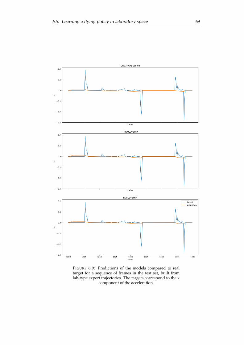
6.5. Learning a flying policy in laboratory space 69

FIGURE 6.9: Predictions of the models compared to realtarget for a sequence of frames in the test set, built fromlab-type expert trajectories. The targets correspond to the x

component of the acceleration.

71

Chapter 7

Hardware and Software

This chapter provides a complete explanation of the different elements thatwere required in order to perform the real experiments. The hardware el-ements described in this chapter are the AR.Drone 2.0 and Optitrack sys-tem, and the software elements that deserve a detailed description are ROS(Robot Operating System) and some of the packages that were used.

7.1 AR.Drone 2.0

During the real experiments, the learned policy has been tested on a real en-vironment, which requires the use of a real quadrotor. The selected droneto fill this role is the AR.Drone 2.0 owned by the Institut de Robòtica i In-formàtica Industrial. The insititute owns other UAVs but this was the onlyone ready to be used in a short-time setup.

The AR.Drone 2.0 is a quadcopter of medium size built by the Frenchcompany Parrot. Some general features of the drone are

• Video recording and photo shooting at 720p and 30FPS.

• Live video streaming.

• Wifi connection.

• Linux 2.6.32 operating system.

• Embedded tag detection for augmented reality games.

and it is equipped with a 3-axis gyroscope, a 3-axis accelerometer, a 3-axis magnetometer, a pressure sensor, an ultrasound sensor for height mea-surements, and a QVGA vertical camera for flight speed measurements.

7.1.1 Mechanical details

The mechanical structure comprises four rotors attached to the four endsof a crossing to which the battery, the motors and the RF hardware are at-tached. Each pair of opposite rotors is turning the same way. To improvestability in flight, one pair is turning clockwise and the other anti-clockwise.By changing the speed of the rotors individually, the drone is able to per-form four fundamental movements, which are vertical linear movement,aka. throttle, and roll, pitch and yaw rotations. The rotor speeds requiredto perform each one of these are illustrated in figure 7.1. The drone is ableto move and rotate in all three dimensions of space by just performing a

72 Chapter 7. Hardware and Software

FIGURE 7.1: The four fundamental movements theAR.Drone is able to perform by individually setting thespeed of the rotors. The magnitude of the blue arrows de-

pict the speed of the rotor

combination of these fundamental movements. Roll and pitch are alwaysused in combination with throttle to move in any direction in the horizontalplane, and only yaw and throttle are in practice applied independently.

The drone has four independent brushless engines which are controlledby a microcontroller that is in charge of transforming the velocity com-mands to the corresponding power signals for the engines. The batterythat was used to provide energy to the drone during the experiments is a1000 mAh and 11.1 volts LiPo battery, whose power level can be tracked inthe display at real time. Finally, all the sensors mentioned above are usedby the internal software of the AR.Drone in order to accurately perform thereceived velocity commands, as well as computing its odometry. It is im-portant to mention that this odometry estimation was not used during theexperiments because it can accumulate significant errors, and instead anOptitrack system was used to estimate the drone’s position with very highaccuracy.

7.2 Optitrack

Optitrack is a motion capture system created by NaturalPoint, Inc. thatallows to locate objects in a bounded space. The system is able to accu-rately locate and track in space special markers by using 10 special camerasthat are built to detect and track the markers. The cameras are placed ina static structure and oriented towards the center, each one recording thescene from a different angle, as figure 7.2 illustrates. This configuration hasthe limitation that the volume in space where the markers can be detectedby the cameras is limited. On the other side, the advantages of Optitrackmotion capture system are that it provides location estimates with less than0.5mm error, and the sensor redundancy allows to track markers that maybe occluded to some cameras.

7.3. Software 73

FIGURE 7.2: Cage structure where the camera sensors aremounted. Note that the cameras record the scene in the cen-

ter of the cage from different angles.

(A) (B) (C)

FIGURE 7.3: Markers applied to A) the AR.Drone, B) themain human protective gear, and C) the obstacle.

The presented Neural Aerial Social Force Model requires certain in-formation about the world that surrounds the drone, that is, it needs toknow the exact location of all the objects that are considered by the model:pedestrian’s positions, obstacle’s positions, main human’s position and thedrone’s position. Since the sensors with which the drone is equipped can-not provide this information, we were forced to use Optitrack to provide allthis information to the NASFM controlling the drone. To do so, the drone,the obstacle and the main human were equipped with several markers, asshown in figure 7.3. As a result, the Optitrack system provided informationabout each element’s position, which was used to build the input of themodel. Information about the orientation was also available but not used.

7.3 Software

7.3.1 FreeGLUT

FreeGLUT is an open source alternative to OpenGL Utility Toolkit libraryand was originally written by Pawel W. Olszta in response to the aban-donment of OpenGL. Essentially, it is a standard specification that defines


a multiplatform and multilanguage API to write software application thatgenerate 2D and 3D graphics. It consists of more than 250 functions that al-low to draw complex structures from simple primitive functions like spheres,cubes, points or lines, as well as manage windows, events, the cursor andother functionalities. It has been used in a wide variety of practical appli-cations because it is simple, widely available and highly portable. It takescare of all the system-specific chores required for creating windows, initial-izing OpenGL contexts, and handling input events, so it provides all therequired features to build a simulator.

Despite existing better simulators, such as gazebo, a simulator was builtusing FreeGLUT, and it was used to record the expert trajectories and testthe learned policies, as explained in 4.1.3 to 4.5. The main reason behindthis decision is that a similar simulator had already been built in FreeGLUTby another IRI researcher, and the present simulator could be built withoutmany effort by introducing some modifications to the previous simulator.We considered that this option would be less time consuming than creatingthe simulator in gazebo from scratch.

7.3.2 Robot Operating System

Robot Operating System was the chosen software tool to implement theNASFM on the real drone because it is the framework used by the IRI andthere are plenty of packages developed specifically for the robots in thelab. ROS is essentially a set of open source software libraries and tools thatease the development of robot applications. It is a robotics middleware thatprovides hardware abstraction, low-level device control, implementationof commonly used functionality, message-passing between processes, andpackage management. The operating system is structured as a graph whereprocessing takes place in nodes, which are simple executables, that may re-ceive, post and multiplex messages from and to other nodes.

Communication in ROS is blackboard based. A node can publish ona particular topic and only the nodes subscribed to that topic are able toreceive the messages. Similarly, services allow communication betweennodes as they allow nodes do send requests and receive responses. In anyROS application there is always a master node whose role is to enable indi-vidual ROS nodes to locate one another. It provides naming and registra-tion services to the rest of the nodes in the system and it tracks publishersand subscribers to topics as well as services. This distributed architectureallows to isolate processing in nodes so that one node can for instance readinformation from sensors and publish the odometry of the robot, while an-other node running a navigation algorithm is subscribed to the odometrymessages. Note that such distribution in the processing provides flexibilityand reusabilty among different robot applications thanks to the use of thestandard messages provided by ROS.

Other relevant tools that ROS provides are rviz and rqt. rviz is a 3Dgraphical interface that allows the visualization of all kinds of sensor data

7.3. Software 75

as well as the robot 3D model at run time. Essentially, it can graphically dis-play the state of the robot and sensors at run time, which can be extremelyuseful in practice. rqt is a framework for developing graphical interfaces fora robot, through several plugins. rqt_graph shows nodes and the connec-tion between them, which allows to easily understand the structure of therunning system. With rqt_plot you can plot and monitor any kind of num-ber that varies over time, such as voltage, velocity or encoders. rqt_topic isused to inspect the topics being published in the system and rqt_publisherallows you to publish your own messages to any topic, facilitating ad-hocexperimentation with your system. Finally, with rqt_bag it is possible torecord data to bags, which can be later replayed at any time.

7.3.3 Gazebo

Gazebo is a 3D dynamic simulator with the ability to accurately and effi-ciently simulate populations of robots in complex indoor and outdoor en-vironments. It includes several powerful features, like high-performancephysics engines, advanced 3D graphics, simulated sensors with the possi-bility to add noise, many robot models, and command line tools. All thesefeatures make Gazebo the best option to quickly evaluate robotic systemsin very realistic simulated environments, which provide a good estimate ofthe performance that can achieved in real environments.

Therefore, we used Gazebo as a second simulator to replicate the condi-tions in the laboratory that will be faced during real experiments, becausethese conditions weren’t met in the FreeGLUT simulator that was used tolearn the expert policies. Using Gazebo, we built a simple environment thatincluded the drone, the main human and an obstacle, and the learned pol-icy was tested by sending the predicted commands to the simulated drone.The drone was simulated in gazebo using the tum_simulator package andthe pedestrian was simulated using the IRI’s object library.

7.3.4 TUM Simulator

The tum_simulator package was written by Hongrong Huang and JuergenSturm of the Computer Vision Group at the Technical University of Mu-nich [2]. The package includes an implementation of the AR.Drone into theGazebo simulator. The package allows to control the AR.Drone in simu-lation as well as in real life, depending on how the package is configured.Figure 7.4 illustrates both simulated and real control architectures of theAR.Drone.

7.3.5 Final NASFM architecture

The implementation of the NASFM on the real robot only involved the cre-ation of a node that runs the neural network controller. This node sim-ply receives the odometry of the different elements in the environment andcomputes the velocity commands to operate the drone. The odometry in-formation may be published by the gazebo simulator, in case the AR.Drone


(A) (B)

FIGURE 7.4: TUM Simulator functional diagram A) in asimulated environment and B) with a real drone.

is being simulated, or it may come from the optitrack node, if a real exper-iment is performed. Thus, the node that implements the learned controllercan be used in both situations without any kind of modification in its code.

The remaining processes required to run the real experiments and thegazebo simulations were already implemented as packages in the IRI repos-itory. Figure 7.5 shows a detailed description of the ROS architectures inboth simulated and real experiments. The node implementing the con-troller is the one named move_drone_node, and it appears in both schemes.The remaining nodes are packages from the IRI repository. The controllernode publishes velocity commands to the node ardrone_area_constrain, whichsimply defines a volume space limiting the space where the drone can fly,and is used to replicate the limits found in the real setup due to optitrack.The output of this node is multiplexed with the output from joystick_teleopto allow the user to control the drone with a joystick, as twist_mux is con-figured to give priority to the commands from the joystick.

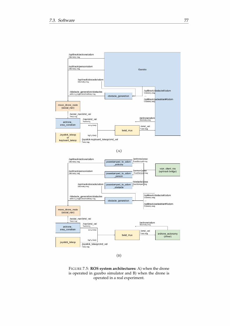
7.3. Software 77

(A)

(B)

FIGURE 7.5: ROS system architectures: A) when the droneis operated in gazebo simulator and B) when the drone is

operated in a real experiment.

79

Chapter 8

Results

This chapter presents all the results obtained during the development of theNASFM. First, the results obtained from testing the learned policies in thesimulated environments are provided. Note that in order to obtain the finalpolicy, several iterations of the learning problem were performed, with in-creasing complexity. The results obtained in each iteration are all presentedin the next section. Additionally, real experiments were performed usingthe policy learned in environments that replicate the laboratory conditions.These results are also presented in the subsequent section.

8.1 Results from simulations

Here, we introduce the obtained policies and the results in the simulatedenvironments.

8.1.1 Policy learned in open space with no obstacles and no pedes-trians

The goal that was established in the first iteration of the learning procedurewas to learn a drone motion policy in an open space without obstacles andbots. To achieve this goal, a dataset was built from recorded expert trajec-tories in this kind of environments. The dataset was used to train the mod-els and test their MSE. This procedure is explained in Section 6.2. In thissection, we present the results that were obtained from testing the learnedpolicies in simulated environments.

Due to the i.i.d assumption violation, the real performance of the mod-els was ultimately assessed in simulated environments, where the trainedmodel provides the control actions given a sensed state of the simulator.In order to get a numeric metric of the overall performance of the policylearned by each model, the performance metric (Section 3.4.6) was com-puted in the 20 test environments corresponding to the test set. This meansthat a total of 80 test environments were simulated. The final performanceachieved by each model was computed as the average of all the perfor-mance measures obtained in the 20 simulated environments. and the val-ues are gathered in table 8.1. The performance of the trajectory provided bythe human expert is also included in the table, in order to give a referenceof the top performance.

From the results provided in table 8.1, we can state that the 3-Layer NNis the model that best imitates the expert policy because its performance

80 Chapter 8. Results

performance A performance BExpert trajectory 0.9236 0.4278

Linear Regression 0.7518 0.27093-Layer NN 0.7935 0.29585-Layer NN 0.7928 0.2225

TABLE 8.1: Final performance average achieved by eachmodel after simulating the learned policies on 10 test en-vironments of type A and 10 test environments of type B.

achieved during the test simulations is on average the highest among thetrained models in both A and B type environments. In A type environmentsthe 5LNN is almost able to match the performance of the 3LNN. However,in B type environments the 5LNN struggles a lot and achieves even lowerperformance than linear regression. The reason for this behaviour is that inthis kind of environments, the drone’s initial position is far from the com-panion, which explains the low performance in general. The movement ofthe drone under the 5LNN control is slower, which results in lower perfor-mance values as it takes longer to approach the companion. So summariz-ing, the control policy learned by the 5LNN is good at flying the drone nextto the companion but is slow at approaching the companion from a far dis-tance.

In conclusion, the obtained results indicate that the 3-layer neural net-work is the best model at learning a flying policy under these conditionsbecause it achieved the highest performance score on average. However,the best learned policy is only slightly better than the worst, the one learnedby linear regression, and it is still far from accurately replicating the experttrajectory.

8.1.2 Policy learned in open space with only pedestrians

After successfully learning the most basic flying policy, we extended thecurrent goal to learn a flying policy such that the drone flies next to the ac-companied person in environments populated with pedestrians but with-out static obstacles. Similarly to the procedure described in the previoussection, a new dataset was built that contains the recordings from experttrajectories in these new environments. A new version of the models wastrained from scratch and their MSE on a test set was computed. This pro-cess is described in Section 6.3.

After training the models, these are evaluated using the performancemetric. In this case, each model is tested on 15 different D-type test envi-ronments and its final performance is computed as the average. Table 8.2gathers the performance results of the controller.

This time, we can see significant differences. First of all, the perfor-mance of the expert trajectory has dropped significantly, which means thatin the new environment conditions the human expert has trouble maintain-ing the drone next to the companion. This can happen because now thecompanion must avoid pedestrians and the resulting path is more complex

8.1. Results from simulations 81

average performanceExpert trajectory 0.7449

Linear Regression 0.67143-Layer NN 0.70575-Layer NN 0.6971

TABLE 8.2: Final performance average achieved by eachmodel after simulating the learned policies on 15 test en-

vironments of type D

and difficult to predict, thus, flying next to the companion is harder. Apartfrom this, the order of the models in terms of performance with respect tothe previous iteration is maintained, which can be expected due to the sim-ilar conditions. The 3-layer NN offers the highest performance, narrowlyfollowed by the 5-layer NN. A significant distance separates linear regres-sion from the neural networks.

In summary, for the second iteration of learning the general flying pol-icy, no changes to the model’s architectures were required in order to trainthem on the new dataset, and the same training procedure was followed.The learned policies were tested on 15 simulated type-D environments inorder to determine the best performing model. Very similar results wereobtained, strengthening the idea that neural networks can learn stable con-trol policies from demonstrations and may provide the best results.

8.1.3 Policy learned in open space populated with obstacles

For the last and final stage in the iterative learning procedure, the goalwas to teach a flying robot to navigate next to the companion in environ-ments that are populated with obstacles of two kinds: columns and bridges.Again, a dataset was built from the expert trajectories this time recorded intwo different kind of environments, K and L, which are explained in moredetail in section 4.1.6. The selected models were, then, trained on thesedatasets and the test MSE was computed, as explained in Section 6.4.

The control policies learned by the models during the training phasewere tested on simulated environments of type L. Additionally, the samepolicies were tested on two different kind of environments that had notbeen seen during training, C and M type environments (sections 4.1.8 and4.1.7). By doing this we are evaluating the generalization capabilities of thelearned policies, which are trained on simpler KL environments and testedon more complex C and M environments.

The performance measurements obtained by simulating the learned poli-cies on environments L, M and C are gathered in table 8.3. As it can be seen,the highest average performance in type L environments is achieved by the3-layer NN, with a significant margin over the second best model, the 5-layer NN. However, the best model is still 0.2 points lower than the expertpolicy. From observing the learned policies’ behaviours during the simula-tion, we know that this significant difference in performance with respect to


L performance M performance C performanceExpert trajectory 0.8563 0.8267 0.8580

Linear Regression 0.5632 0.4771 0.62203-Layer NN 0.6586 0.5481 0.72565-Layer NN 0.6088 0.5459 0.7196


vironments of type L, 15 of type M and 10 of type C.

the expert trajectory comes from the fact that although the learned policiesare able to successfully avoid obstacles, they do it slower and tend to fallbehind the companion.

Regarding the performance measurements obtained in M type environ-ments, in general there is a slight loss of performance with respect to Lenvironments, which could be explained by the fact that M environmentscontain the same kind of obstacles than the training environments but inlarger amounts, hindering the navigation task. Another important thing tomention is that the performance of both neural networks are very similar,even though the 3-layer NN is still the best.

Finally, the models’ performances achieved in C type environments arein general higher than the measurements in L environments because C en-vironments only contain tree obstacles, and the density of objects is lower,thus the space between objects is larger, making the navigation task easier.The performances of the neural networks are again very similar, but the3-layer NN is still better.

8.1.4 Policy learned in spaces replicating laboratory conditions

As it has been said in previous sections, it is not suitable to implement thepolicies learned in open spaces populated with obstacles in the real exper-iments. The main reason is that the conditions in the laboratory are signif-icantly different that those found in the simulated environments on whichthe final policies are learned. The observed behaviour of the policies is ex-pected to be suboptimal due to the different distribution of the input. Tosolve this issue, a new set of simulated environments was built, new experttrajectories were recorded, a new dataset was built and the models weretrained again from scratch, using this new dataset. The full procedure isexplained in section 6.5.

After computing the test MSE of the trained models in order to verifythat the training process was completed, the learned policies were simu-lated on the 16 test environments of type lab, the performance metric wascomputed in each one and then averaged over all 16 test environments. Theresulting values of performance are gathered in table 8.4.

The results are consistent with all previous results in terms of the bestperforming model, which is the 3-layer NN. The performance it achievesis significantly higher than those obtained by the 5-layer NN and Linear

8.2. Results from real experiments 83

average performanceExpert trajectory 0.5920

Linear Regression 0.44133-Layer NN 0.47025-Layer NN 0.4438


vironments of type lab.

Regression, which are actually very similar. However, the best performingpolicy is still far from replicating the expert policy, as they are separated bymore than a 12% difference.

8.1.5 Conclusion

In the last iteration of the learning procedure the goal was to learn the finalflying control policy that would allow the drone to safely fly side-by-sidewith a human companion in environments populated with pedestrians andobstacles. This requires the drone to learn two different behaviours: (1) tofly next to a human companion and (2) to avoid collisions with static ob-stacles as well as dynamic obstacles, represented by other pedestrians. Thefirst behaviour was successfully learned in the first two iterations of theglobal learning procedure. Learning the second behaviour was addressedin this section.

At the beginning of this section we explained that it was not possible tolearn effective control policies from expert trajectories recorded in C and Menvironments. Therefore, it was not possible to learn a controller to nav-igate in these environments just from expert trajectories recorded in theseenvironments. Consequently, we simplified the environments to K and Ltypes, where the number of obstacles was reduced to one of each kind perenvironment, and trained the models on them. The results showed that itwas possible to learn effective control policies to safely navigate in theseenvironments, as shown in the first column of table 8.3.

Motivated by this success, we then tested these learned policies on Cand M type environments and the results were surprisingly good. As thesecond and third columns of table 8.3 indicate, all models are able to safelynavigate the drone in the unseen environments (M and C), with differentdegrees of effectiveness. This result has a remarkable implication because itmeans that it is more efficient to learn the policy in simplified versions of theenvironment where the robot is going to be deployed, instead of learningthe policy directly from the deploying environment.

8.2 Results from real experiments

This section describes the implementation of the policy learned in lab en-vironments into the AR.Drone, the simulations of the NASFM on gazebo,and finally the results from the real tests performed in the laboratory.


8.2.1 Implementation of the model on the AR.Drone

The results provided in the previous section show that the best policy in labenvironments corresponds to the 3-layer NN. Therefore, this was the cho-sen model to be implemented on the real drone.

The implementation of the controller consists in building a ROS node,which is subscribed to the odometry of the different elements in the envi-ronment and publishes velocity commands, as illustrated in figure 7.5. Thenode, named in the figure as move_drone_node, is unique and can be usedboth in the gazebo simulator or in the real drone. The rest of the nodes arealready implemented in the repository of the IRI.

Internally, the controller node has a C++ description of the 3-layer NN,which is used to compute the acceleration predictions given a standard-ized input. The input is built from the odometry of the different elementsin the environment that is available each cycle, and the corresponding ac-celeration prediction is transformed to velocity and published. The librarykeras2cpp [3] was used to translate the neural network model from kears toC++. The controller node also include the human path prediction moduleand the collision detection module. Similarly, the neural network mod-els implementing each model were translated from keras to C++ using thesame library.

8.2.2 Simulating lab policy in Gazebo

Once the implementation of the controller node had been completed, wetested the policy trained in lab environments on the gazebo simulator. Itis important to note that the gazebo simulator is significantly different toFreeGLUT simulator, which was used for training the models, because gazeboincludes a complex physics engine that simulates the dynamics of the AR.Dronemodel.

The observed behaviour of the drone on the gazebo simulator was sig-nificantly different than the one observed in FreeGLUT simulator, eventhough the same environment configuration was used. In gazebo, the dronereacts slower and it shows wider oscillations. In some cases the collisiondetection module does not predict properly and the drone collides with theobstacle. The human path prediction module, on the other hand, worksfine.

In general, the observed behaviour of the drone in gazebo simulator isworse than in FreeGLUT simulator. A possible explanation for such resultwould be the differences introduced in gazebo, mainly the simulation ofthe AR.Drone dynamics. The introduction of the drone’s dynamics mayintroduce noise in the odometry of the drone, because the dynamic modelonly applies the velocity commands that are physically feasible, given theparameters of the drone. In general, this effect would smooth the result-ing drone’s odometry, affecting the input of future cycles of the controller.

8.2. Results from real experiments 85

FIGURE 8.1: Simulated environment in gazebo replicatingthe conditions found in the laboratory. The drone, the mainhuman and an obstacle are the only elements in the envi-

ronment, which is also limited by the green volume.

FIGURE 8.2: Pictures taken during the real experiments,where the learned policy is tested on the real drone.

Figure 8.1 shows one of the simulated environments in gazebo, which sim-ulates the environment’s conditions.

8.2.3 Running the control policy on the real drone

The behaviour of the control policy observed in gazebo was not promising,so we were a little skeptical to try it on the real drone. At the end, we de-cided to give it a try because the twist_mux node allows to take control ofthe drone at any point, avoiding any possible disaster.

First of all, the optitrack node was configured in order to identify eachcluster of markers to each element in the environment, the human protec-tive gear, the AR.Drone and the obstacle, as shown in figure 7.3. With this,the optitrack node can accurately publish the odometry of each element.Then, the whole ROS architecture described in Figure 7.5 (b) was launched,the drone was taken of, and its control was given to the ROS node imple-menting the NASFM. Figure 8.2 provides several pictures of the real exper-iments performed in the laboratory.


The behavour of the drone observed in the real experiments was bad,in the sense that several characteristics of the behaviour exhibited in FreeG-LUT simualtor were not observed on the real drone. In first place, the heightof the drone was incorrect, because it was trained to fly above the head ofthe person, but as figure 8.2 shows, it never happened in the real experi-ments. In second place, the drone was unable to stay still next to the personif the person was staying still. The drone exhibited a constant drift in somedirection that would lead it to exit the bounded volume or to collide withthe obstacle. Lastly the drone was not able to avoid collisions with the ob-stacle and, although it did not collide with the human, the drone was notkeeping a safe distance to the human, and approached him too much.

In conclusion, the observed behaviour of the drone on real experimentswas bad, and worse than the observed behaviour of the drone in gazebosimulator, but still it was not terrible. Overall, the motion of the drone wasslow, which allowed us to safely apply corrections when the integrity ofthe drone was at risk. We inspected the internal functioning of the internalnode and concluded that the velocity commands published by the droneare so small that in a real scenario they are surpassed by the drift inherentto the drone, and the fact that the policy has a feedback loop propagates theerror and makes it worse.

87

Chapter 9

Conclusions

The overall goal of the work presented in this thesis is to teach a learningmodel a control policy to fly a drone just from demonstrations provided byan expert in simulated environments. This can be divided into two consec-utive subgoals: (1) to learn a flying policy from expert trajectories recordedin simulated environments that behaves correctly when applied in the samekind of simulated environments; and (2), to check that the policy trained insimulated environments provides a good behaviour when applied on a realdrone in a real environment.

We begin the chapter with a brief recall of the main objective of thepresent work, as well as its decomposition in its subgoals. Then, we dis-cuss the degree in which each subgoal has been accomplished, providingempirical evidence to support our statements. Finally, we evaluate quanti-tatively the overall success of the presented NASFM.

9.1 Learning and effective policy for simulated envi-ronments

Regarding the first subgoal, Section 8.1 provides evidence that the task tolearn a flying control policy that behaves successfully in simulated environ-ments has been achieved. It took several stages of learning, each one morecomplex than the previous, but the policy learned in the final stage showeda satisfactory behaviour, even in an environment type that was not seen atthe training phase. This iterative approach of learning policies with increas-ing difficulty was taken after failing at learning a complete control policy incomplex environments. At the beginning, we had no idea about the mech-anisms and the way the models learn useful policies from demonstrations.Therefore, we decided to make the problem easier by learning individualaspects of the complete policy.

First of all, we forced the models to learn a control policy to just flynext to the main human, in environments without obstacles and bots, asdescribed in Section 6.2. After training the models, the policies were testedon simulated environments of the same kind and the performance metricwas used to assess the performance of each model. The results shown inSection 8.1.1 confirm that this simple policy was successfully learned.

88 Chapter 9. Conclusions

We then set the new goal of learning a flying policy in open spaces withonly pedestrians, with the added complexity of having pedestrians wan-dering in the environment (Section 6.3). This policy turned out to be verysimilar to the previous one, and it was easily learned as results from Section8.1.2 show. From this learning stage, we concluded that pedestrians can beeasily avoided by just flying higher than their heads, which is a trivial pol-icy to learn.

Finally, we included the interaction of obstacles into the training envi-ronments, which turned out to be the most challenging stage of all. We firsttried to learn a policy in C-type environments (Section 4.5), but we failed.As a consequence of this initial failure, we simplified the environment intotype K (Section 4.3), we trained the models from scratch on expert trajec-tories recorded in these environments and tested the learned policies insimulations. The observed behaviour was effective at avoiding the columnobstacle. After that, we built new environments that included a bridge ob-stacle, labeled as L-type (Section 4.3), we trained again the models on thesenew environments and tested the learned policies on simulations. The ob-served behaviour was able to successfully avoid bridges and column obsta-cles, as shown by the performance metric values in table 8.3.

In the past, we failed at trying to learn a policy in complex environ-ments, such as C or M types. Therefore, we did not begin a new trainingstage in more complex environments. Instead, we just took the policieslearned in K and L types and tested them in C and M environments. Theobserved behaviour was quite surprising because the drone was able tonavigate in these more complex environments, avoiding column and bridgeobstacles. We computed the performance achieved in each type of environ-ment, as listed in table 8.3. Furthermore, in C environments, the drone wassafely accompanying the main human, even though these environmentscontain tree obstacles, which are not present in K and L environments.

Overall, these results show that the tested models have remarkable gen-eralization abilities, even for the linear regression model. Additionally, weconclude that it is better to learn policies in simple environments and expectgood generalization in more complex ones.

9.2 Learning and effective policy for a real drone

The results from the experiments performed on the FreeGLUT simulatorprove that the proposed NASFM is able to control a drone so that it fliesside-by-side with a human in simulated environments with pedestriansand different kinds of obstacles. The next step is to check the validityof NASFM when the learned policy is implemented on a real drone. Toachieve this, a ROS node was created that implements the NASFM with allits modules: the module that predicts acceleration commands, the collisiondetection module and the human path prediction module. Once the node isbuilt, it can be tested on Gazebo simulator before trying it on the real UAV,in this case an AR.Drone.

9.3. Final conclusions 89

Thus, first of all, we implemented the best performing policy learned inK and L environments on the ROS controller node and tested it in Gazebo.The observed behaviour was significantly worse than the one observed inFreeGLUT simulator. We thought that this result could be explained by thefact that the environment simualted in Gazebo, which replicates the con-ditions in the laboratory, was significantly different than the environmentsused to train the policy.

In order to solve this issue, we built new environments replicating lab-oratory conditions, on which we trained new models. We then simulatedthe new learned policies on test environments and checked that they wereeffective. Finally, we implemented the best model on the controller nodeand tested it in Gazebo. The observed behaviour was slightly better, butstill wasn’t as good as the behaviour observed in FreeGLUT simulator.

At this point, we got to the conclusion that maybe the dynamic modelsimulator inside Gazebo was causing the problem. The simulator has acomplex physics engine, and TUM Simulator that contains the Gazebo modelof the AR.Drone has a description of the dynamics of the drone. The con-troller node published velocity commands to Gazebo, which applies themto update the simulator state. If a commands is not physically feasible dueto the limitations of the drone, the simulator does not update the system ac-cording to the velocity commands. This introduces noise into the feedbackloop that is present in the drone’s controller, modifying the distribution ofthe input. We believe that this effect is responsible for the behaviour ob-served in Gazebo, where the drone moves slower and looses agility.

Even though the behaviour of NASFM in Gazebo was not particularlygood, we still tried it on the real drone. As we expected, the behaviourof the AR.Drone in the real experiments was unsatisfactory. Firstly, thedrone was unable to fly above the head of the person, even though it didin Gazebo. Secondly, the drone was unable to stay still next to the person ifthe person was staying still, showing a constant drift in some direction thatwould lead it to exit the bounded volume or to collide with the obstacle.Lastly the drone was not able to avoid collisions with the obstacle, and itwas approaching the human too much.

We concluded that probably the issue with the dynamics of the droneare worsened in real experiments due to the noise in the odometry estima-tion and execution of velocity commands. Additionally, we inspected thevelocity commands and saw that they took generally small values, whichare surpassed by the drift inherent to the real drone.

9.3 Final conclusions

As it is explained in the previous sections, we have successfully learned acontrol policy for a drone to fly next to a human that works well in simu-lated environments. However, we have not been able to obtain an equallygood behaviour in real life experiments.

90 Chapter 9. Conclusions

We believe that the acceleration prediction model lacks robustness, be-cause it is severely affected by modification in its feedback loop. This is animportant issue because in real applications we expect to find significantnoise introduced to the feedback loop.

In general the limitations of NASFM have a lot to do with Learning fromDemonstrations. In FreeGLUT simulator there is no physics engine andthe predicted acceleration commands are executes as they are. This affectsthe process of policy testing as well as the process of trajectory recording.It is possible that the recorded trajectories include some actions that arephysically unfeasible but are learned by the models. When these modelsare tested on FreeGLUT simulator, their behaviour is good because they aretested on the same conditions where they are trained. However, in a realscenario, the models may have learned impossible actions, which producea different feedback when performed, and thus the distribution of the inputis different, violating the i.i.d. assumption.

91

Chapter 10

Future work

As it has been explained in the Conclusions chapter, we consider that thetask of learning a control policy that behaves correctly in real environmentshas not been successfully achieved. While this result is disappointing, wecan still take advantage of the situation by listing the limitations of the workand providing ideas that could possibly improve the NASFM, based on theinsight gained during the development of this thesis.

10.1 Limitations of the current work

The results obtained in real experiments show that the present NASFM hasseveral limitations.

In first place, the system relies heavily on the Neural Network modelthat is in charge of computing the acceleration commands. The movementof the drone is entirely defined by the predictions of the model, with theonly exception being the moment when a collision is detected. In this casea correction is applied to the prediction that forces an avoidance action.This heavy dependency on the model’s prediction makes the whole systemvery fragile to errors of the model, as made evident in the real experiments.If the conditions found in the real world are different from those found inthe simulator, due to noise and physical limitations, the system is at risk offailing completely, as there are no mechanisms that prevent it. Addition-ally, the collision detection module is also based on a Neural Network, sothe same reasoning applies.

A second limitation of the present work that we believe is a source oferror is the fact that test conditions don’t match the final application’s con-ditions. This concept is fundamental in Machine Learning, and states thatin order for the performance metric to be meaningful, it must be assessedon a test that comes from the same distribution that is expected to be foundin the final application. In the present work, the performance metric is com-puted on test environments simulated in FreeGLUT because the training setis recorded in this simulator. However, FreeGLUT simulator is very idealand it doesn’t even have a physics engine. This makes the performancemeasurements not representative of the expected final performance in realexperiments. In our defence, however, we must say that collecting the ex-pert trajectories in real environments was unfeasible, as it would have re-quired too much effort and time. Therefore, we decided to collect the experttrajectories in simulated environments.

92 Chapter 10. Future work

Finally, we consider the dataset size as the last limitation of the presentwork. There is no way to know exactly to which degree a larger datasetwould have improved the performance of the system, but it definitely wouldhave helped. A larger dataset is more likely to cover a larger portion of thefeature space, which would result in better models. This issue may be par-ticularly critical in the case of Learning from Demonstrations, as errors canbe propagated quadratically in time [50]. The final policies built in thiswork were trained in datasets of 70 to 110 minutes of expert demonstra-tions, which can be considered as a small dataset. A larger dataset wouldhave helped but still wouldn’t have made much of a difference.

10.2 Next steps

From all the discussion and analysis of the limitations of NASFM, we havecome up with several ideas that could improve different aspects of the ap-proach. However, all these are out of the scope of the thesis and are pre-sented below a next steps.

In order to make the learned policies more robust, a possible improve-ment could be to remove the Drone Velocity feature. The problem with thisfeature is that it represents the current velocity of the drone, and it can beseverely affected when NASFM is tested on a real drone. In real experi-ments, we have observed that the drone tends to move when it should not,due to stabilization issues. This undesired movement introduces significantnoise into this feature, which has a dramatic impact on the predictions ofthe model. Additionally, the model relies too much on the velocity feature,because a safe policy is to always predict accelerations that produce smallchanges to the feature, for continuity reasons. Therefore, we believe that byremoving the velocity feature these limitations would disappear.

Regarding the issue with the test conditions that do not match the finalapplication, the obvious improvement would be to record the expert trajec-tories directly with the real drone. However, we understand that this canbe very costly, so as an intermediate solution we propose the use of Gazebofor recording the example trajectories. Gazebo includes a physics engine,which added to the available model of the AR.Drone, provides a significantimprovement with respect to FreeGLUT. If special attention is addressed toreplicating the real condition found in the laboratory, the performance ofthe tested models will be a better estimate of the real performance of thedrone.

As a general improvement, we suggest to rely less on the learned policyto govern the motion of the drone. With the Learning from Demonstrationsapproach, there is always going to be the risk of undesired behaviour. Itmay seem that the system always works fine, but there is no guarantee thatthe system will behave adequately if it reaches an unseen state. The reasonbehind this is that the learned policy is based on a Neural Network, whichis seen as a black box. Currently, there is still no way to fully comprehendthe mechanisms that are involved in the computation of the network’s out-put. Maybe a hybrid approach would be better, one in which the network

10.2. Next steps 93

control actions at a higher level, and there is a lower level mechanism thatperforms the commands from the network, reliably translating them intoadequate actions.

Finally, we would like to mention that the problem can be tackled by acompletely different approach. Note that this is not an improvement, in-stead, it is a complete shift in perspective with a fundamentally differentsolution. The main problem addressed in this thesis fits naturally into theset of problems usually considered in Reinforcement Learning paradigm. Re-inforcement Learning deals essentially with the task of learning the best action toperform in different situations. The task is formulated as maximizing the rewardreceived in long term by balancing exploitation of actions whose reward is knownand exploration of new action whose reward is not accurately known. The problemof learning a control policy for a drone that must fly side-by-side with a human canbe seen as learning the best action to choose in each possible state of the environ-ment, which naturally fits Reinforcement Learning’s problem formulation.

95

Bibliography

[1] URL: http://freeglut.sourceforge.net.

[2] URL: http://wiki.ros.org/tum_simulator.

[3] URL: https://github.com/pplonski/keras2cpp.

[4] Antoine Bautin, Luis Martinez-gomez, and Thierry Fraichard. “In-evitable Collision States : a Probabilistic Perspective”. In: IEEE Inter-national Conference on Robotics and Automation (2010), pp. 4022–4027.

[5] Maren Bennewitz et al. “Learning Motion Patterns of People for Com-pliant Robot Motion”. In: The International Journal of Robotics Research24.1 (2005), pp. 31–48.

[6] N. Bu, M. Okamoto, and T. Tsuji. “A Hybrid Motion ClassificationApproach for EMG-Based Human–Robot Interfaces Using Bayesianand Neural Networks”. In: IEEE Transactions on Robotics 25.3 (2009),pp. 502–511. ISSN: 1552-3098.

[7] Cauchard, Jessica R and Jane, L E and Zhai, Kevin Y and Landay,James A. “Drone & Me : An Exploration Into Natural Human - DroneInteraction”. In: 2015 ACM International Joint Conference on Pervasiveand Ubiquitous Computing. ACM. 2015, pp. 361–365.

[8] Cauchard, Jessica R and Zhai, Kevin Y and Spadafora, Marco andLanday, James A. “Emotion Encoding in Human-Drone Interaction”.In: ACM/IEEE International Conference on Human Robot Interaction. ACM/IEEE.2016, pp. 263–270.

[9] Zhuo Chen, Lu Wang, and Nelson H.C. Yung. “Adaptive human mo-tion analysis and prediction”. In: Pattern Recognition 44.12 (2011), pp. 2902–2914. ISSN: 0031-3203.

[10] Gonçalo Charters Santos Cruz and Pedro Miguel Martins Encarnação.“Obstacle Avoidance for Unmanned Aerial Vehicles”. In: Journal of In-telligent & Robotic Systems 65.1-4 (2011), pp. 203–217. ISSN: 0921-0296.

[11] H. Dee and D. Hogg. “Detecting inexplicable behaviour”. In: BritishMachine Vision Conference (2004).

[12] Desaraju, V and Ro, H C and Yang, M and Tay, E and Roth, S and Vec-chio, D Del. “Partial Order Techniques for Vehicle Collision Avoid-ance : Application to an Autonomous Roundabout Test-bed”. In: IEEEInternational Conference on Robotics and Automation,2009. ICRA ’09. IEEE.2009, pp. 263–270.

[13] Mihai Duguleana and Gheorghe Mogan. “Neural networks based re-inforcement learning for mobile robots obstacle avoidance”. In: ExpertSystems With Applications 62 (2016), pp. 104–115. ISSN: 0957-4174.

[14] D. Bank E. Prassler and B. Kluge. “Key technologies in robot assis-tants: Motion coordination between a human and a mobile robot”. In:Transactions on Control, Automation and Systems Engineer- ing (2002).

http://freeglut.sourceforge.net

http://wiki.ros.org/tum_simulator

https://github.com/pplonski/keras2cpp

96 BIBLIOGRAPHY

[15] Luis Alberto GARZA ELIZONDO. “Social-aware Drone Navigationusing Social Force Model”. MA thesis. Barcelona School of Informat-ics, 2016.

[16] A.G Fallis. “Probabilistic robotics”. In: Journal of Chemical Informationand Modeling 53.9 (2013), pp. 1689–1699. ISSN: 1098-6596.

[17] Fahimi Farbod. Autonomous Robots:modeling, path planning, and control.2005. ISBN: 9780387095370.

[18] Gonzalo Ferrer and Alberto Sanfeliu. “Comparative Analysis of Hu-man Motion Trajectory Prediction Using Minimum Variance Curva-ture”. In: Proceedings of the 6th International Conference on Human-robotInteraction. HRI ’11. Lausanne, Switzerland: ACM, 2011, pp. 135–136.ISBN: 978-1-4503-0561-7.

[19] Amalia F. Foka and Panos E. Trahanias. “Probabilistic AutonomousRobot Navigation in Dynamic Environments with Human MotionPrediction”. In: International Journal of Social Robotics 2.1 (2010), pp. 79–94. ISSN: 1875-4805.

[20] Friedman, Jerome and Hastie, Trevor and Tibshirani, Robert. The Ele-ments of Statistical Learning: Data Mining , Inference and Prediction. 2008.

[21] D. Gandhi, L. Pinto, and A. Gupta. “Learning to fly by crashing”. In:2017 IEEE/RSJ International Conference on Intelligent Robots and Systems(IROS). 2017, pp. 3948–3955.

[22] García-Delgado, L. A. and Noriega, J. R. and Berman-Mendoza, D.and Leal-Cruz, A. L. and Vera-Marquina, A. and Gómez-Fuentes, R.and García-Juárez, A. and Rojas-Hernández, A. G. and Zaldívar-Huerta,I. E. “Repulsive Function in Potential Field Based Control with Algo-rithm for Safer Avoidance”. In: Journal of Intelligent & Robotic Systems80.1 (2015), pp. 59–70. ISSN: 0921-0296.

[23] Gardiner, Ben and Ahmad, W and Cooper, T and Haveard, M. “Colli-sion Avoidance Techniques for Unmanned Aerial Vehicles TechnicalReport# CSSE11-01”. In: Techniques (2011), pp. 1–24.

[24] A. Garrell. “Cooperative social robots: accompanying, guiding andinteracting with people”. In: (2013).

[25] A. Garrell et al. “Aerial social force model: A new framework to ac-company people using autonomous flying robots”. In: 2017 IEEE/RSJInternational Conference on Intelligent Robots and Systems (IROS). 2017,pp. 7011–7017.

[26] A. Garrell et al. “Teaching robot’s proactive behavior using human as-sistance”. In: International Journal of Social Robotics 9.2 (2017), pp. 231–249.

[27] A. Giusti et al. “A Machine Learning Approach to Visual Perceptionof Forest Trails for Mobile Robots”. In: IEEE Robotics and AutomationLetters 1.2 (2016), pp. 661–667.

[28] Edward Twitchell Hall. The Hidden Dimension. 1966.

[29] Dan He. “FlyingBuddy : Augment Human Mobility and Perceptibil-ity”. In: International conference on Ubiquitous Computing (2011), pp. 615–616.

BIBLIOGRAPHY 97

[30] Dirk Helbing and Péter Molnár. Social force model for pedestrian dynam-ics. 1995.

[31] O. Khatib. “Real-time obstacle avoidance for manipulators and mo-bile robots”. In: 2 (1985), pp. 500–505.

[32] Dong Ki Kim and Tsuhan Chen. “Deep Neural Network for Real-Time Autonomous Indoor Navigation”. In: CoRR abs/ 1511.04668 (2015).arXiv: 1511.04668.

[33] Kwang-Yeon Kim, Jung-Woo Park, and Min-Jea Tahk. “UAV collisionavoidance using probabilistic method in 3-D”. In: (2007), pp. 826–829.

[34] Diederik P. Kingma and Jimmy Ba. “Adam: A Method for StochasticOptimization”. In: CoRR abs/1412.6980 (2014). arXiv: 1412.6980.

[35] Thibault Kruse et al. “Human-aware robot navigation : A survey”.In: Robotics and Autonomous Systems 61.12 (2013), pp. 1726–1743. ISSN:0921-8890.

[36] D. N. Lee. “Guiding movements by coupling taus”. In: Ecological Psy-chology 10 (1998), 221–250.

[37] Guanghui Li et al. “An efficient improved artificial potential fieldbased regression search method for robot path planning”. In: 2012IEEE International Conference on Mechatronics and Automation, ICMA2012 (2012), pp. 1227–1232.

[38] Ming Lin. “Reciprocal Velocity Obstacles for Real-Time Multi-AgentNavigation”. In: IEEE International Conference on Robotics and Automa-tion (2008), pp. 1928–1935.

[39] A. Loquercio et al. “DroNet: Learning to Fly by Driving”. In: IEEERobotics and Automation Letters 3.2 (2018), pp. 1088–1095.

[40] Jan R Magnus and Wendun Wang. “Weighted-average least squaresprediction â^—”. In: (2013), pp. 1–38. ISSN: 15324168.

[41] Julieta Martinez, Michael J. Black, and Javier Romero. “On humanmotion prediction using recurrent neural networks”. In: CoRR abs/1705.02445 (2017).

[42] Vicente Matellán Olivera and Reid Simmons. “Implementing human-acceptable navigational behavior and fuzzy controller for an autonomousrobot”. In: Workshop en Agentes Físicos, Marzo, 2002, Murcia, España(2002).

[43] Florian Mueller and Matthew Muirhead. “Understanding the Designof a Flying Jogging Companion”. In: Proceedings of the Adjunct Publi-cation of the 27th Annual ACM Symposium on User Interface Software andTechnology. UIST’14 Adjunct. Honolulu, Hawaii, USA: ACM, 2014,pp. 81–82. ISBN: 978-1-4503-3068-8.

[44] Nagi, Jawad and Giusti, Alessandro and Caro, Gianni A Di and Gam-bardella, Luca M. “Human Control of UAVs using Face Pose Esti-mates and Hand Gestures”. In: ACM/IEEE International Conference onHuman-Robot Interaction c (2014), pp. 252–253.

[45] Yasushi Nakauchi and Reid Simmons. “A Social Robot that Stands inLine”. In: Autonomous Robots 12.3 (2002), pp. 313–324. ISSN: 1573-7527.

http://arxiv.org/abs/1511.04668


98 BIBLIOGRAPHY

[46] Tayyab Naseer. “FollowMe : Person Following and Gesture Recog-nition with a Quadrocopter”. In: IEEE/RSJ International Conference onIntelligent Robots and Systems (IROS) (2013), pp. 624–630.

[47] I. R. Nourbakhsh, C. Kunz, and T. Willeke. “The mobot museum robotinstallations: a five year experiment”. In: Proceedings 2003 IEEE/RSJInternational Conference on Intelligent Robots and Systems (IROS 2003)(Cat. No.03CH37453). Vol. 4. 2003, 3636–3641 vol.3.

[48] Jason M. O’Kane and Jason M. O. Kane. A gentle introduction to ROS.2013, p. 155. ISBN: 978-1492143239.

[49] T. Kanda T. Miyashita P. Althaus H. Ishiguro and H.I. Christensen.“Navigation for human-robot interaction tasks”. In: Proceedings of theIEEE International Conference on Robotics and Automation ().

[50] Stephane Ross, Geoffrey Gordon, and Drew Bagnell. “A Reductionof Imitation Learning and Structured Prediction to No-Regret On-line Learning”. In: Proceedings of the Fourteenth International Conferenceon Artificial Intelligence and Statistics. Ed. by Geoffrey Gordon, DavidDunson, and Miroslav Dudík. Vol. 15. Proceedings of Machine Learn-ing Research. Fort Lauderdale, FL, USA: PMLR, 2011, pp. 627–635.

[51] Y. Manabe Y. Nakami T. Takamori S. Tadokoro M. Hayashi. “On mo-tion planning of mobile robots which coexist and cooperate with hu-man”. In: IEEE/RSJ International Conference on Intelligent Robots andSystems (1995).

[52] Fereshteh Sadeghi and Sergey Levine. “(CAD)$ˆ2$RL: Real Single-Image Flight without a Single Real Image”. In: CoRR abs/1611.04201(2016). arXiv: 1611.04201.

[53] Weisberg Sanford. Applied Linear Regression. 2005. ISBN: 0-471-66379-4.

[54] Satoru Satake et al. “How to Approach Humans?-Strategies for So-cial Robots to Initiate Interaction-”. In: Journal of the Robotics Society ofJapan 28.3 (2010), pp. 327–337. ISSN: 0289-1824.

[55] Stefan Schneegass et al. “Midair Displays : Concept and First Expe-riences with Free-Floating Pervasive Displays”. In: International Sym-posium on Pervasive Displays (2014), pp. 1–5.

[56] Wai Shan, Florence Ng, and Ehud Sharlin. “Collocated Interactionwith Flying Robots”. In: IEEE International Symposium on Robot andHuman Interactive Communication (2011).

[57] Reid Simmons. “The Curvature-Velocity Method for Local ObstacleAvoidance”. In: IEEE International Conference on Robotics and Automa-tion April (1996).

[58] Nikolai Smolyanskiy et al. “Toward Low-Flying Autonomous MAVTrail Navigation using Deep Neural Networks for Environmental Aware-ness”. In: CoRR abs/1705.02550 (2017).

[59] Emma Sviestins et al. “Speed Adaptation for a Robot Walking witha Human”. In: Proceedings of the ACM/IEEE International Conferenceon Human-robot Interaction. HRI ’07. Arlington, Virginia, USA: ACM,2007, pp. 349–356. ISBN: 978-1-59593-617-2.


BIBLIOGRAPHY 99

[60] Daniel Szafir et al. “Communication of Intent in Assistive Free Fly-ers”. In: ACM/IEEE international conference on Human-robot interaction2.1 (2014), pp. 358–365.

[61] S. Thrun et al. “MINERVA: a second-generation museum tour-guiderobot”. In: Proceedings 1999 IEEE International Conference on Roboticsand Automation (Cat. No.99CH36288C). Vol. 3. 1999, 1999–2005 vol.3.

[62] N. E. Du Toit and J. W. Burdick. “Probabilistic Collision CheckingWith Chance Constraints”. In: IEEE Transactions on Robotics 27.4 (2011),pp. 809–815. ISSN: 1552-3098.

[63] Dieter Fox Dirk Hähnel Gerhard Lakemeyer Dirk Schulz Walter SteinerWolfram Burgard Armin B Cremers and Sebastian Thrun. “Experi-ences with an interactive museum tour-guide robot”. In: Artificial in-telligence (1999).

[64] M. Zhang et al. “Dynamic artificial potential field based multi-robotformation control”. In: (2010), pp. 1530–1534. ISSN: 1091-5281.

[65] T. Zhang et al. “Learning deep control policies for autonomous aerialvehicles with MPC-guided policy search”. In: (2016), pp. 528–535.

[66] Zhu, Lihua and Cheng, Xianghong and Yuan, Fuh Gwo. “A 3D col-lision avoidance strategy for UAV with physical constraints”. In: Mea-surement: Journal of the International Measurement Confederation 77 (2016),pp. 40–49. ISSN: 02632241.

[67] B. D. Ziebart et al. “Planning-based prediction for pedestrians”. In:2009 IEEE/RSJ International Conference on Intelligent Robots and Sys-tems. 2009, pp. 3931–3936.

Neural Aerial Social Force Model: Teaching a Drone to ...

Documents

Transcript of Neural Aerial Social Force Model: Teaching a Drone to ...