Network-level Optimization for Unbalanced Power Distribution … · Challenges: Network-level...

Network-level Optimization for Unbalanced Power Distribution Systems

Anamika DubeyAssistant Professor (EECS)

Washington State University, Pullman([email protected])

PSERC WebinarSeptember 24, 2019

1

Presentation Outline

2

• Motivation

• Challenges

• Proposed Approach

• Approximation and Relaxation Techniques

• Applications

• Future Research Directions

Motivation: Network-level Optimization

3

Modern Power Grid:• Distributed and Non-dispatchable

Generation • Bidirectional power flow• Controllable loads/Prosumers• Generation Variability and

Uncertainty Industrial Loads

Step-down

Sub-transmission customer

Step-down

Generating Station Step-upDistribution Substation

Bulk Transmission

Residential/Commercialcustomers

Renewables Park

Key drivers for Network-level Optimization in Power Distribution Systems: • Incorporate non-traditional resources (DERs, responsive loads, battery storage),• Incorporate controllable loads – smart buildings/prosumers,• Incorporate new measurements and other sources of data,• Increased requirement for power quality and reliability, • Ensure resilience to disasters.

• More data • More control• More communication

Network-level optimization to harness the new capabilities

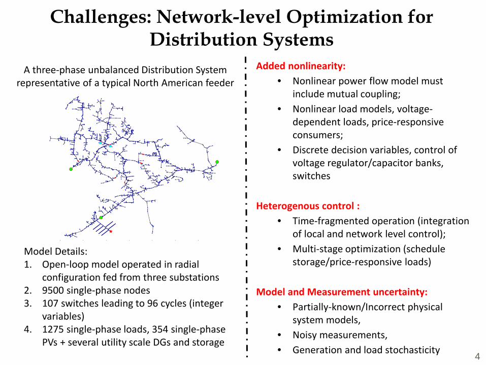
Challenges: Network-level Optimization for Distribution Systems

4

Model Details: 1. Open-loop model operated in radial

configuration fed from three substations2. 9500 single-phase nodes3. 107 switches leading to 96 cycles (integer

variables)4. 1275 single-phase loads, 354 single-phase

PVs + several utility scale DGs and storage

A three-phase unbalanced Distribution System representative of a typical North American feeder

Added nonlinearity: • Nonlinear power flow model must

include mutual coupling;• Nonlinear load models, voltage-

dependent loads, price-responsive consumers;

• Discrete decision variables, control of voltage regulator/capacitor banks, switches

Heterogenous control : • Time-fragmented operation (integration

of local and network level control); • Multi-stage optimization (schedule

storage/price-responsive loads)

Model and Measurement uncertainty: • Partially-known/Incorrect physical

system models, • Noisy measurements, • Generation and load stochasticity

This Talk: Network-level Optimization for Unbalanced Distribution Systems

5

My Research:

• Optimal power flow algorithms for unbalanced power distribution systems.

• Proposed methods for scalable optimal power flow algorithms for large-scale distribution systems.

• Application of OPF model for distribution grid operational challenges.

Specific Applications:

• Conservation voltage reduction. (Method) Scalable three-phase optimal power flow with mixed-integer constraints.

• Network topology estimation. (Method) Estimating network topology (normal and outaged) that satisfies the measurements. Formulated as a network-level optimization problem with discrete decision variables.

• Resilient Restoration with intentional islanding. (Method) Optimal reconfiguration while meeting dynamic island feasibility considerations for improved resilience to natural disasters.

6

Branch power flow model*

* L. Gan and S. H. Low, "Convex relaxations and linear approximation for optimal power flow in multiphase radial networks," 2014 Power Systems Computation Conference, Wroclaw, 2014, pp. 1-9.

objective: 𝑚𝑚𝑚𝑚𝑚𝑚 𝑓𝑓(𝑥𝑥)

subject to: 𝑔𝑔 𝑥𝑥 = 𝑏𝑏

For ex. Conservation voltage reduction, Loss minimization, etc.

Power flow equations, operating constraints

Non-convex OPF model

Non-convex OPF model of reduced

complexity

Approximate power flow model

Iterative Convex OPF

Iterative Linearized OPF

Approximation Relaxation

My Research

𝑣𝑣𝑗𝑗 = 𝑣𝑣𝑖𝑖 + 𝑧𝑧𝑖𝑖𝑗𝑗𝑙𝑙𝑖𝑖𝑗𝑗𝑧𝑧𝑖𝑖𝑗𝑗𝐻𝐻 − 𝑍𝑍𝑖𝑖𝑗𝑗𝑆𝑆𝑖𝑖𝑗𝑗𝐻𝐻 − 𝑆𝑆𝑖𝑖𝑗𝑗𝑍𝑍𝑖𝑖𝑗𝑗𝐻𝐻

𝑑𝑑𝑚𝑚𝑑𝑑𝑔𝑔 𝑆𝑆𝑖𝑖𝑗𝑗 − 𝑧𝑧𝑖𝑖𝑗𝑗𝐼𝐼𝑖𝑖𝑗𝑗𝐼𝐼𝑖𝑖𝑗𝑗𝐻𝐻 − 𝑠𝑠𝑗𝑗 = 𝑑𝑑𝑚𝑚𝑑𝑑𝑔𝑔 (𝑆𝑆𝑗𝑗𝑗𝑗)

𝑣𝑣𝑖𝑖 𝑆𝑆𝑖𝑖𝑗𝑗𝑆𝑆𝑖𝑖𝑗𝑗𝐻𝐻 𝑙𝑙𝑖𝑖𝑗𝑗

=𝑉𝑉𝑖𝑖𝐼𝐼𝑖𝑖𝑗𝑗

𝑉𝑉𝑖𝑖𝐼𝐼𝑖𝑖𝑗𝑗

𝐻𝐻


:- Rank -1 PSD matrix

Network-level Optimization: Three-Phase Optimal Power Flow (OPF)

Network-level Optimization: Reducing Complexity - Three-Phase Power Flow Model

7

Assumptions :1. The phase voltages are assumed to approximately 120◦ degree apart.

2. The phase angle difference (𝛿𝛿𝑖𝑖𝑗𝑗𝑝𝑝𝑝𝑝 ) between branch currents are obtained from

equivalent constant impedance model

𝑉𝑉𝑖𝑖𝑎𝑎

𝑉𝑉𝑖𝑖𝑏𝑏≈𝑉𝑉𝑖𝑖𝑏𝑏

𝑉𝑉𝑖𝑖𝑐𝑐≈𝑉𝑉𝑖𝑖𝑐𝑐

𝑉𝑉𝑖𝑖𝑎𝑎≈ 𝑒𝑒𝑗𝑗𝑗𝑗𝑗/3

Via

Vib

Vic

𝑉𝑉𝑖𝑖𝑎𝑎 ≠ 𝑉𝑉𝑖𝑖𝑏𝑏 ≠ 𝑉𝑉𝑖𝑖𝑐𝑐

i j

Equivalent Z model

Ĩij∠δij

ZIP

i jIij∠δij

δijab

Iija

Iijb

Iijc

Ĩija

Ĩijb

Ĩijc

δijab

δij is approximated in OPF. Iij is a variable in OPF

Validation of Assumptions

Test Feeder % Load error in 𝜹𝜹𝒊𝒊𝒊𝒊𝒑𝒑𝒑𝒑 (degrees) error in 𝜽𝜽𝒊𝒊

𝒑𝒑𝒑𝒑(degrees)

IEEE 13 bus 75 % 1.8 1.8

IEEE 13 bus 100 % 2.1 2.2

IEEE 123 bus 75 % 0.8 0.9

IEEE 123 bus 100 % 1.13 1.3

Feeder- R3-12.47-2 75 % 0.5 0.55

Feeder- R3-12.47-2 100 % 0.9 1.05

8

• The power flow is solved in OpenDSS at various loading condition fordifferent test feeder

• 𝜃𝜃𝑖𝑖𝑝𝑝𝑝𝑝 is the phase angle difference between node voltage and 𝛿𝛿𝑖𝑖

𝑝𝑝𝑝𝑝 is thephase angle difference between branch currents

• The results shows the maximum error in 𝜃𝜃𝑖𝑖𝑝𝑝𝑝𝑝 and 𝛿𝛿𝑖𝑖

𝑝𝑝𝑝𝑝 for a test feeder

Nonlinear Power Flow Equations (Linear)

𝑃𝑃𝑖𝑖𝑗𝑗𝑝𝑝𝑝𝑝 − 𝑝𝑝𝐿𝐿𝑗𝑗

𝑝𝑝 = �𝑗𝑗:𝑗𝑗→𝑗𝑗

𝑃𝑃𝑗𝑗𝑗𝑗𝑝𝑝𝑝𝑝 − �

𝑝𝑝𝜖𝜖𝜑𝜑𝑗𝑗

𝑙𝑙𝑖𝑖𝑗𝑗𝑝𝑝𝑝𝑝 𝑟𝑟𝑖𝑖𝑗𝑗

𝑝𝑝𝑝𝑝 cos 𝛿𝛿𝑖𝑖𝑗𝑗𝑝𝑝𝑝𝑝 − 𝑥𝑥𝑖𝑖𝑗𝑗

𝑝𝑝𝑝𝑝 sin 𝛿𝛿𝑖𝑖𝑗𝑗𝑝𝑝𝑝𝑝

𝑄𝑄𝑖𝑖𝑗𝑗𝑝𝑝𝑝𝑝 − 𝑞𝑞𝐿𝐿𝑗𝑗


𝑄𝑄𝑗𝑗𝑗𝑗𝑝𝑝𝑝𝑝 − �


𝑙𝑙𝑖𝑖𝑗𝑗𝑝𝑝𝑝𝑝 𝑥𝑥𝑖𝑖𝑗𝑗

𝑝𝑝𝑝𝑝 cos 𝛿𝛿𝑖𝑖𝑗𝑗𝑝𝑝𝑝𝑝 + 𝑟𝑟𝑖𝑖𝑗𝑗


𝑣𝑣𝑗𝑗𝑝𝑝= 𝑣𝑣𝑖𝑖

𝑝𝑝 − �𝑝𝑝∈𝜑𝜑𝑗𝑗

2ℝ𝑒𝑒 𝑆𝑆𝑖𝑖𝑗𝑗𝑝𝑝𝑝𝑝 𝑍𝑍𝑖𝑖𝑗𝑗

𝑝𝑝𝑝𝑝 𝐻𝐻+ �


𝑍𝑍𝑖𝑖𝑗𝑗𝑝𝑝𝑝𝑝𝑙𝑙𝑖𝑖𝑗𝑗

𝑝𝑝𝑝𝑝 + �𝑝𝑝1,𝑝𝑝𝑗∈𝜑𝜑𝑗𝑗,𝑝𝑝1≠𝑝𝑝𝑗

2ℝ𝑒𝑒 𝑍𝑍𝑖𝑖𝑗𝑗𝑝𝑝𝑝𝑝1𝑙𝑙𝑖𝑖𝑗𝑗

𝑝𝑝1𝑝𝑝𝑗 ∠𝛿𝛿𝑖𝑖𝑗𝑗𝑝𝑝1𝑝𝑝𝑗 𝑧𝑧𝑖𝑖𝑗𝑗

𝑝𝑝𝑝𝑝𝑗 𝐻𝐻

(Quadratic)

𝑃𝑃𝑖𝑖𝑗𝑗𝑝𝑝𝑝𝑝 𝑗

+ 𝑄𝑄𝑖𝑖𝑗𝑗𝑝𝑝𝑝𝑝 𝑗

= 𝑣𝑣𝑖𝑖𝑝𝑝𝑙𝑙𝑖𝑖𝑗𝑗𝑝𝑝𝑝𝑝

𝑙𝑙𝑖𝑖𝑗𝑗𝑝𝑝𝑝𝑝 𝑗

= 𝑙𝑙𝑖𝑖𝑗𝑗𝑝𝑝𝑝𝑝𝑙𝑙𝑖𝑖𝑗𝑗

𝑝𝑝𝑝𝑝

9



Network-level Optimization: Three-Phase Optimal Power Flow of Reduced Complexity

Validation of Power Flow

10

Largest Error in Nonlinear Power Flow wrt. OpenDSS Solutions

• The total number of variables in the proposed formulation are 15 × (n − 1), where n is the number of nodes; the original branch-flow based models had a total of 36 × (n − 1) variables.

• Computational time to solve NLP model for conservation voltage reduction objective in MATLAB using fmincon: o IEEE 13-bus – 20 sec, o IEEE 123-bus (267 single-phase nodes) – 4 min, o Feeder- R3-12.47-2 (860 single-phase nodes) – 20 min.

Accurate but still not scalable for large systems

Test Feeder % loading Pflow (%) Qflow (%) Sflow (%) V(pu)

IEEE 13 Bus 100 % 0.29 2.03 0.253 0.003

IEEE 123 Bus 100 % 0.61 3.88 0.286 0.002

Feeder- R3-12.47-2 100 % 0.6 3.4 0.163 0.0002

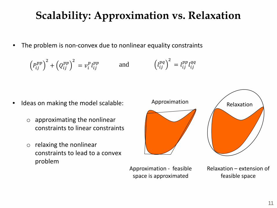
Scalability: Approximation vs. Relaxation

11

Approximation - feasible space is approximated

• The problem is non-convex due to nonlinear equality constraints



𝑝𝑝𝑝𝑝𝑃𝑃𝑖𝑖𝑗𝑗𝑝𝑝𝑝𝑝 𝑗


= 𝑣𝑣𝑖𝑖𝑝𝑝𝑙𝑙𝑖𝑖𝑗𝑗𝑝𝑝𝑝𝑝 and

• Ideas on making the model scalable:

o approximating the nonlinear constraints to linear constraints

o relaxing the nonlinear constraints to lead to a convex problem

Relaxation – extension of feasible space

Approximation

AC

Relaxation

Three-Phase Optimal Power Flow (OPF)

12









complexity





My Research






𝐻𝐻



𝑃𝑃𝑖𝑖𝑗𝑗𝑝𝑝𝑝𝑝 − 𝑝𝑝𝐿𝐿𝑗𝑗


𝑃𝑃𝑗𝑗𝑗𝑗𝑝𝑝𝑝𝑝 − �


𝑙𝑙𝑖𝑖𝑗𝑗𝑝𝑝𝑝𝑝 𝑟𝑟𝑖𝑖𝑗𝑗

𝑝𝑝𝑝𝑝 cos 𝛿𝛿𝑖𝑖𝑗𝑗𝑝𝑝𝑝𝑝 − 𝑥𝑥𝑖𝑖𝑗𝑗


𝑄𝑄𝑖𝑖𝑗𝑗𝑝𝑝𝑝𝑝 − 𝑞𝑞𝐿𝐿𝑗𝑗


𝑄𝑄𝑗𝑗𝑗𝑗𝑝𝑝𝑝𝑝 − �


𝑙𝑙𝑖𝑖𝑗𝑗𝑝𝑝𝑝𝑝 𝑥𝑥𝑖𝑖𝑗𝑗

𝑝𝑝𝑝𝑝 cos 𝛿𝛿𝑖𝑖𝑗𝑗𝑝𝑝𝑝𝑝 + 𝑟𝑟𝑖𝑖𝑗𝑗


𝑣𝑣𝑗𝑗𝑝𝑝 = 𝑣𝑣𝑖𝑖

𝑝𝑝 − �𝑝𝑝∈𝜑𝜑𝑗𝑗

2ℝ𝑒𝑒 𝑆𝑆𝑖𝑖𝑗𝑗𝑝𝑝𝑝𝑝 𝑍𝑍𝑖𝑖𝑗𝑗

𝑝𝑝𝑝𝑝 𝐻𝐻+ �


𝑍𝑍𝑖𝑖𝑗𝑗𝑝𝑝𝑝𝑝𝑙𝑙𝑖𝑖𝑗𝑗

𝑝𝑝𝑝𝑝 + �𝑝𝑝1,𝑝𝑝𝑗∈𝜑𝜑𝑗𝑗,𝑝𝑝1≠𝑝𝑝𝑗

2ℝ𝑒𝑒 𝑍𝑍𝑖𝑖𝑗𝑗𝑝𝑝𝑝𝑝1𝑙𝑙𝑖𝑖𝑗𝑗

𝑝𝑝1𝑝𝑝𝑗 ∠𝛿𝛿𝑖𝑖𝑗𝑗𝑝𝑝1𝑝𝑝𝑗 𝑧𝑧𝑖𝑖𝑗𝑗

𝑝𝑝𝑝𝑝𝑗 𝐻𝐻






𝑝𝑝𝑝𝑝

Relaxation: General Model

13

• Can be relaxed to a second-order cone-constraint: Convex problem (SOCP)

• After relaxation

• The relaxation however was found to be not exact

Iterative approach to reach the feasible solution over multiple iterations of the

SOCP relaxed problem

• Additional constraint is defined to reduce feasibility gap

𝑒𝑒1 = 𝑣𝑣𝑖𝑖𝑝𝑝𝑙𝑙𝑖𝑖𝑗𝑗𝑝𝑝𝑝𝑝 − 𝑃𝑃𝑖𝑖𝑗𝑗

𝑝𝑝𝑝𝑝2 − 𝑄𝑄𝑖𝑖𝑗𝑗𝑝𝑝𝑝𝑝2

𝑒𝑒2 = 𝑙𝑙𝑖𝑖𝑗𝑗𝑝𝑝𝑝𝑝 ∗ 𝑙𝑙𝑖𝑖𝑗𝑗

𝑝𝑝𝑝𝑝 − 𝑙𝑙𝑖𝑖𝑗𝑗𝑝𝑝𝑝𝑝2

Nonlinear equations in OPF model

𝑣𝑣𝑖𝑖𝑝𝑝𝑙𝑙𝑖𝑖𝑗𝑗𝑝𝑝𝑝𝑝 ≥ 𝑃𝑃𝑖𝑖𝑗𝑗

𝑝𝑝𝑝𝑝2 + 𝑄𝑄𝑖𝑖𝑗𝑗𝑝𝑝𝑝𝑝2

𝑙𝑙𝑖𝑖𝑗𝑗𝑝𝑝𝑝𝑝 ∗ 𝑙𝑙𝑖𝑖𝑗𝑗

𝑝𝑝𝑝𝑝 ≥ 𝑙𝑙𝑖𝑖𝑗𝑗𝑝𝑝𝑝𝑝2

• The power flow will have solution on the surface of the cone.

• Convex Relaxation - The nonlinear equality constraints are converted into inequality constraints thus expanding the feasible space to the interior of the cone:

• Feasibility gap is defined as

Relaxation – Understanding Feasibility Gap

14



≤ 𝑣𝑣𝑖𝑖𝑝𝑝𝑙𝑙𝑖𝑖𝑗𝑗𝑝𝑝𝑝𝑝

c1

high v

c2

low v

l

q

p

• For minimization problem (for ex. loss minimization) the solution for the relaxed model is known to lie at the surface of the cone under certain conditions that are usually satisfied by the single-phase network.

• Thus, the solution of relaxed problem is exact as it lies on the surface of the cone.

Single-phase radial distribution feeder

𝑒𝑒𝑟𝑟𝑟𝑟𝑒𝑒𝑟𝑟 = 𝑣𝑣𝑖𝑖𝑝𝑝𝑙𝑙𝑖𝑖𝑗𝑗𝑝𝑝𝑝𝑝 − 𝑃𝑃𝑖𝑖𝑗𝑗


S. H. Low, “Convex relaxation of optimal power flow Part I: Formulations and equivalence,” IEEE Transactions on Control of Network Systems, vol. 1, no. 1, pp. 15–27, March 2014.

Relaxation – Understanding Feasibility Gap

15

• For maximization problem (for ex. maximum PV hosting), the relaxed solution was found to be inexact.

• In this case, the relaxed problem can have optimal solution inside the cone.

• Here, for the relaxed problem the solution obtained is 𝑐𝑐𝑟𝑟 which is optimal for SOCP but infeasible for actual problem leading to feasibility gap.

l

q

p

voltage constraintinfeasible solution

c1

cr

c2

cf

We enforce a linear inequality constraint to reduce the feasibility

gap over successive iterations of the relaxed problem*.

Single-phase radial distribution feeder

𝑒𝑒𝑟𝑟𝑟𝑟𝑒𝑒𝑟𝑟 = 𝑣𝑣𝑖𝑖𝑝𝑝𝑙𝑙𝑖𝑖𝑗𝑗𝑝𝑝𝑝𝑝 − 𝑃𝑃𝑖𝑖𝑗𝑗


*Rahul Ranjan Jha and Anamika Dubey, “Exact Distribution Optimal Power Flow (D-OPF) Model using Convex Iteration Technique,” accepted to appear at 2019 IEEE PES General Meeting.

Approach: Iterative Second-order Cone Programming for Three-phase OPF

16

• An iterative approach that solves multiple iterations of SOCP relaxed problems to drive the solution to feasible space.

• Feasibility gap termed as error is defined as

• Added linear inequality constraints that minimizes the feasibility gap in successive SOCP iterations.

e2(k) = 𝑙𝑙𝑖𝑖𝑗𝑗

𝑝𝑝𝑝𝑝(𝑗𝑗) ∗ 𝑙𝑙𝑖𝑖𝑗𝑗𝑝𝑝𝑝𝑝(𝑗𝑗) − 𝑙𝑙𝑖𝑖𝑗𝑗

𝑝𝑝𝑝𝑝(𝑗𝑗) 𝑗

e1(k) = 𝑣𝑣𝑖𝑖

𝑝𝑝 𝑗𝑗 𝑙𝑙𝑖𝑖𝑗𝑗𝑝𝑝𝑝𝑝 𝑗𝑗 − 𝑃𝑃𝑖𝑖𝑗𝑗

𝑝𝑝𝑝𝑝 𝑗𝑗 𝑗− 𝑄𝑄𝑖𝑖𝑗𝑗

𝑝𝑝𝑝𝑝(𝑗𝑗) 𝑗

Is errork < tol ?Yes

Stop

xk+1 = xk + Δx

Starttol = 10-4, k = 1

Solve linearized optimal power flow flin(x) = 0,

xk = xlin

Solve SOCP (with added directional constraint) for Δx

No

k = k+1

17

Test feeder Loadingcondition

Computation time (NLP)

Computationtime (SOCP)

IEEE 13 bus minimum 17.95 sec 4.00 sec

IEEE 13 bus maximum 13.51 sec ~20.0 sec(10 iterations)

IEEE 123 bus minimum ~2 min 30.00 sec(8 iteration)

IEEE 123 bus maximum ~4 min 40.00 sec(10 iteration)

The computation time required for each iteration to solve the IEEE-123 node system using CVX is approximately 4.00 sec

Results: Iterative SOCP for Three-phase Power Distribution System

IEEE-123 bus test systemIEEE-13 bus test system

5 10 15 20 25

iteration number

0

0.05

0.1

0.15

max

imum

erro

r

5 10 15 20 25 30

iteration number

0

0.1

0.2

0.3

0.4

0.5

max

imum

erro

r

Feasibility Gap: e𝑟𝑟𝑟𝑟𝑒𝑒𝑟𝑟 = max 𝑣𝑣𝑖𝑖𝑙𝑙𝑖𝑖𝑗𝑗 − (𝑃𝑃𝑖𝑖𝑗𝑗𝑗 + 𝑄𝑄𝑖𝑖𝑗𝑗𝑗 ) , 𝑙𝑙𝑖𝑖𝑗𝑗𝑝𝑝 𝑙𝑙𝑖𝑖𝑗𝑗

𝑝𝑝 − 𝐼𝐼𝑖𝑖𝑗𝑗𝑝𝑝𝑝𝑝 𝑗

Three-Phase Optimal Power Flow (OPF)

18









complexity





My Research






𝐻𝐻



Approximation: General Model

19

Nonlinear program general form𝑚𝑚𝑚𝑚𝑚𝑚 𝑓𝑓(𝑥𝑥)𝑠𝑠𝑠𝑠 𝑔𝑔 𝑥𝑥 = 𝑏𝑏

Penalty Successive Linear Programming:𝑚𝑚𝑚𝑚𝑚𝑚 𝑓𝑓 𝑥𝑥𝑗𝑗 + 𝛻𝛻𝑓𝑓 ∆𝑥𝑥 + 𝑤𝑤 ∑𝑖𝑖 𝑝𝑝𝑖𝑖 + 𝑚𝑚𝑖𝑖𝑠𝑠𝑠𝑠 𝑔𝑔𝑖𝑖 𝑥𝑥𝑗𝑗 + 𝛻𝛻𝑔𝑔𝑖𝑖∆𝑥𝑥 − 𝑏𝑏𝑖𝑖 = 𝑝𝑝𝑖𝑖 − 𝑚𝑚𝑖𝑖

−𝑠𝑠𝑗𝑗 ≤ ∆𝑥𝑥 ≤ 𝑠𝑠𝑗𝑗

𝑙𝑙 ≤ 𝑥𝑥𝑗𝑗 + ∆𝑥𝑥 ≤ 𝑢𝑢𝑝𝑝𝑖𝑖 ≥ 0, 𝑚𝑚𝑖𝑖 ≥ 0






𝑝𝑝𝑝𝑝

Nonlinear equations in OPF model • Nonlinear quadratic equations• Linearized around optimal

operating point obtained from linearized three-phase OPF model

• Solves within 3-4 iterations of linear programming

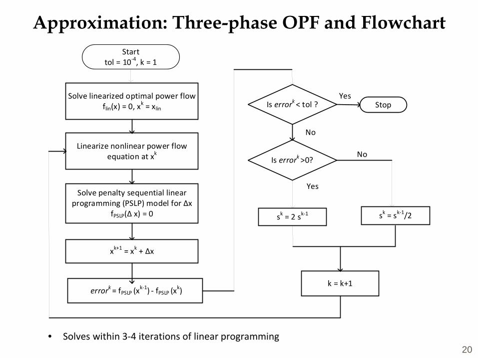
Approximation: Three-phase OPF and Flowchart

20• Solves within 3-4 iterations of linear programming

Yes

No

Stop

xk+1 = xk + Δx

errork = fPSLP (xk-1) - fPSLP (xk)

Starttol = 10-4, k = 1

Solve linearized optimal power flow flin(x) = 0, xk = xlin

Linearize nonlinear power flow equation at xk

Solve penalty sequential linear programming (PSLP) model for Δx

fPSLP(Δ x) = 0

k = k+1

sk = 2 sk-1

Yes

No

Is errork < tol ?

Is errork >0?

sk = sk-1/2

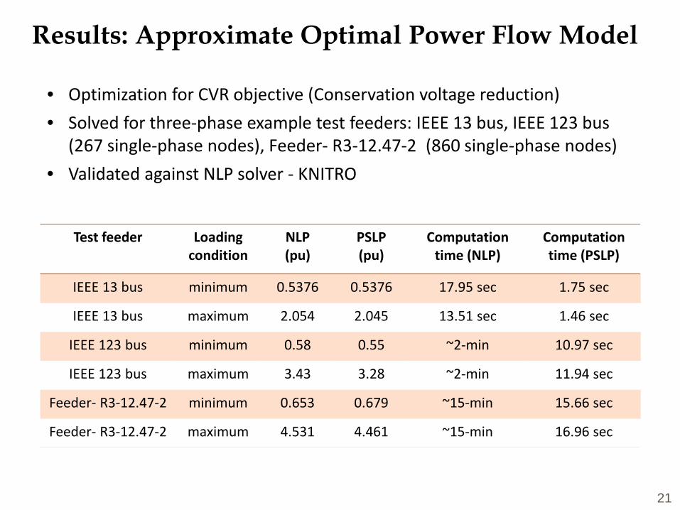
Results: Approximate Optimal Power Flow Model

21

Test feeder Loadingcondition

NLP (pu)

PSLP (pu)

Computation time (NLP)

Computationtime (PSLP)

IEEE 13 bus minimum 0.5376 0.5376 17.95 sec 1.75 sec

IEEE 13 bus maximum 2.054 2.045 13.51 sec 1.46 sec

IEEE 123 bus minimum 0.58 0.55 ~2-min 10.97 sec

IEEE 123 bus maximum 3.43 3.28 ~2-min 11.94 sec

Feeder- R3-12.47-2 minimum 0.653 0.679 ~15-min 15.66 sec

Feeder- R3-12.47-2 maximum 4.531 4.461 ~15-min 16.96 sec

• Optimization for CVR objective (Conservation voltage reduction)• Solved for three-phase example test feeders: IEEE 13 bus, IEEE 123 bus

(267 single-phase nodes), Feeder- R3-12.47-2 (860 single-phase nodes) • Validated against NLP solver - KNITRO

Applications

Application 1 - Conservation voltage reductionMethod: Scalable three-phase optimal power flow with mixed-integer constraints.

Application 2 - Topology estimation: during normal and outage condition Method: Estimation for topology that satisfies power flow measurements. Formulated as a network-level optimization problem.

Application 3 - Resilient Restoration with intentional islanding Method: Optimal reconfiguration while meeting dynamic island feasibility considerations for improved resilience to natural disasters.

22

Application 1: Conservation Voltage Reduction/Volt-VAR Optimization

23

Customer1 Customer NCustomer2

1

2

N

distance

voltage (pu)

0.95

1.05

distance

voltage (pu)

0.95

1.05

Customer1 Customer NCustomer2

1 2 N

Volt-VAr Optimization

Control signals

Without Volt-VAR Optimization (VVO)

Coordinated control grid’s legacy devices (voltage regulator, capacitor banks) and new devices (smart inverters) to reduce feeder voltages and thereby demand from feeder’s voltage-dependent loads.

With Volt-VAR Optimization (VVO)

Application 1: Volt-VAR Optimization

24

Approach - Using network-level optimization to coordinate legacy devices and smart inverters and meet objectives of conservation voltage reduction. • Mathematically problem is formulated as mixed integer nonlinear program (MINLP) • Mixed integer due to discrete and continuous variables and nonlinear due to three-

phase nonlinear power flow.

Rahul Ranjan Jha, Anamika Dubey, Chen-Ching Liu, Kevin, P. Schneider, “Bi-Level Volt-VAR Optimization to Coordinate Smart Inverters with Voltage Control Devices,” accepted IEEE Transactions on Power Systems, Jan. 2019

Level 1: Mixed integer linear programming (MILP)Objective function: 𝑚𝑚𝑚𝑚𝑚𝑚 ∑𝑝𝑝∈𝜑𝜑𝑠𝑠 𝑃𝑃𝑠𝑠

𝑝𝑝(𝑠𝑠)Subject to: linear power flow, voltage regulator control, capacitor bank control,voltage limits, and reactive power limits on DGsControl variables: Regulator tap (𝐴𝐴𝑝𝑝(𝑠𝑠)) , capacitor (𝑢𝑢𝑖𝑖 𝑠𝑠 ) and DG reactive power (𝑄𝑄𝐷𝐷𝐷𝐷)

Fix the status of Regulator tap (𝐴𝐴𝑝𝑝(𝑠𝑠)) , capacitor switch (𝑢𝑢𝑖𝑖 𝑠𝑠 )

Level 2: Nonlinear programming (NLP)Objective function: 𝑚𝑚𝑚𝑚𝑚𝑚 ∑𝑝𝑝∈𝜑𝜑𝑠𝑠 𝑃𝑃𝑠𝑠

𝑝𝑝(𝑠𝑠)Subject to: non-linear power flow , voltage limits, and reactive power limits on DGsControl variables: reactive power from DG (𝑄𝑄𝐷𝐷𝐷𝐷)

Application 1: Volt-VAR Optimization: Results

1

34

5 6

27 8

12

11 14

10

20 19

2221

18 3537

40

135

3332

31

2726

2528

29 30250

48 4749 50

51

4445

46

42

43

41

36 38 39

66

65 64

63

62

60 160 67575859

545352 55 5613

34

1516

1796

95

94

93

152

92 90 88

91 89 87 86

80

81

82 83

84

788572

7374

75

7779

300111 110

108109 107

112 113 114

105106

101102

103104

450100

97

99

6869

7071

197

151

150

61 610 9

24

23

251

451

149

98

76

Nodes with DG

DG2

DG1

DG3

VR1

VR2

VR3

VR4

Nodes with Capacitor

3Φ C1

1Φ C2 1Φ C3 1Φ C4

• Total number of single-phase nodes in this unbalanced system = 267

• Control Devices: 4 Voltage regulators, 4 capacitor banks, and 9 distributed generators

IEEE-123 bus system

• Without CVR controlo VR and capacitor banks are working

autonomously and PVs operating at unity power factor

• With CVR Controlo Reduction in power consumption

from substationo Higher reduction in power demand

at minimum loading condition

26

• Total number of single-phase nodes in this unbalanced system = 860

• Control Devices: 1 Voltage regulator, 4 capacitor banks, and 9 distributed generators

PNNL-329 bus system

Vs

Node with DG

Node with Capacitor

VR1

Application 1: Volt-VAR Optimization: Results

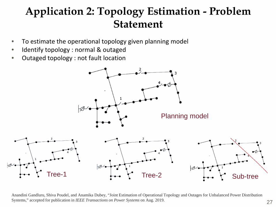
Application 2: Topology Estimation - Problem Statement

27

Planning model

Tree-1 Tree-2 Sub-tree

Anandini Gandluru, Shiva Poudel, and Anamika Dubey, “Joint Estimation of Operational Topology and Outages for Unbalanced Power Distribution Systems,” accepted for publication in IEEE Transactions on Power Systems on Aug. 2019.

• To estimate the operational topology given planning model• Identify topology : normal & outaged• Outaged topology : not fault location

Application 2: Topology Estimation

28

Approach - Use network-level optimization to estimate the switch statuses using erroneous measurements.• Formulated as an estimation problem• Measurements used flow, load, and

smart meter ping measurements

Measurement Error Model• Errors in continuous measurements (flow and load):

• Errors in Smart Meter Ping Measurements (discrete):

• Sum of Errors in Smart Meter Ping Measurements (Gaussian Approximation)

𝑒𝑒 �𝑃𝑃𝑖𝑖𝑗𝑗𝜑𝜑 ~𝑁𝑁 0,𝜎𝜎�𝑃𝑃𝑖𝑖𝑗𝑗

𝜑𝜑𝑗 and 𝑒𝑒 �𝑄𝑄𝑖𝑖𝑗𝑗

𝜑𝜑 ~𝑁𝑁 0,𝜎𝜎�𝑄𝑄𝑖𝑖𝑗𝑗𝜑𝜑𝑗

𝑒𝑒( �𝑦𝑦𝑗𝑗) = ( �𝑦𝑦𝑗𝑗 − 𝑦𝑦𝑙𝑙)~𝐵𝐵𝑒𝑒𝑟𝑟𝑚𝑚𝑒𝑒𝑢𝑢𝑙𝑙𝑙𝑙𝑚𝑚 𝑞𝑞𝑞𝑞 = 𝑃𝑃 ( �𝑦𝑦𝑗𝑗−𝑦𝑦𝑙𝑙) = 1

Minimize �𝜑𝜑∈{𝑎𝑎,𝑏𝑏,𝑐𝑐}

�𝑗𝑗∈𝐼𝐼

�̂�𝑠𝐿𝐿𝑗𝑗𝜑𝜑 − 𝑠𝑠𝐿𝐿𝑗𝑗

𝜑𝜑

𝜎𝜎𝑠𝑠𝐿𝐿𝑗𝑗𝜑𝜑

+ �𝑖𝑖𝑗𝑗∈𝐵𝐵

�̂�𝑆𝑖𝑖𝑗𝑗𝜑𝜑 − 𝑆𝑆𝑖𝑖𝑗𝑗

𝜑𝜑

𝜎𝜎𝑆𝑆𝑖𝑖𝑗𝑗𝜑𝜑

Error in load variables and load measurements Error in flow variable and flow measurements. • Power balance constraints • Radial topology • Error bounds on Smart Meter ping measurements

𝑆𝑆𝑛𝑛𝑝𝑝~𝐵𝐵 𝑚𝑚𝑝𝑝,𝑞𝑞 → 𝑆𝑆𝑛𝑛𝑝𝑝~𝑁𝑁 𝜇𝜇𝑒𝑒,𝜎𝜎𝑒𝑒

𝜇𝜇𝑒𝑒 = 𝑚𝑚𝑝𝑝𝑞𝑞 ; 𝜎𝜎𝑒𝑒 = 𝑚𝑚𝑝𝑝𝑞𝑞(1− 𝑞𝑞)

Application 2: Topology Estimation - Results

29

Model Characteristics:• Four-feeder 1069 nodes• Each feeder:

o 40 sectionalizing switcheso Three 1-𝜙𝜙 and one 3−𝜙𝜙 Capacitor

• Seven tie-switches• Large number of possible operating topologies

Detailed Feeder

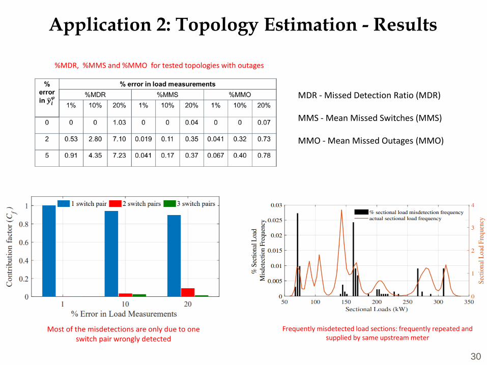
Application 2: Topology Estimation - Results

30

Frequently misdetected load sections: frequently repeated and supplied by same upstream meter

Most of the misdetections are only due to one switch pair wrongly detected

%MDR, %MMS and %MMO for tested topologies with outages

MDR - Missed Detection Ratio (MDR)

MMS - Mean Missed Switches (MMS)

MMO - Mean Missed Outages (MMO)

Application 3: Resilient Restoration (Problem)

31

Restoration during Extreme Events• Distribution feeder disconnected from

main grid• Distribution system itself under stress• Restore critical loads as soon as possible• DERs can be utilized for supplying the CLs• Combinatorial problem – large number of

options to restore the network using all available resources

Critical Loads

1

3 4

5 6

2 7 8

12

11 14

10

20 19

22 21

18 35

37

40

135

33 32

31

27 26

25 28

29 30

250

48 47 49 50

51

44 45 46

42

43

41

36 38 39

66

65 64

63

62

60 160 67

57 58 59

54 53 52 55 56

13

34

15

16

17 96

95

94

93

152

92 90 88

91 89 87 86

80

81

82 83

84

78 85 72

73 74

75

77 79

300 111 110

108 109 107

112 113 114

105

106

101

102 103

104 450

100

97

99

68 69

70 71

197

151

150

61 610 9

24

23

251

195

451

149

350

76

98

76

Fault

G

P Q

Main grid

Earthquake

HurricaneTsunami

Flood

Tornado

Tie-Switches

PV

WT

PV

ES

ESMT

WT

WT

WT

PV

PV

ES

ES

MT

DERs

Distribution system after a natural disaster

Power distribution system restoration using backup feeders and available DER. The out-of-service area is restored with suitable switching scheme after the fault has been isolated

Service Restoration • Transmission and distribution network

remain intact• Single fault due to component failure• No stochastic feature involved in general

analysis• DERs and backup feeders can be utilized

for supplying the outaged loads• Quickly repair and restore

Application 3: Resilient Restoration - Approach

32

Approach - Use network-level optimization to maximize the total load restored using all available resources: feeders, DGs (intentional islanding), smart switches, legacy voltage control devices.

Critical Loads

1

3 4

5 6

2 7 8

12

11 14

10

20 19

22 21

18 35

37

40

135

33 32

31

27 26

25 28

29 30

250

48 47 49 50

51

44 45 46

42

43

41

36 38 39

66

65 64

63

62

60 160 67

57 58 59

54 53 52 55 56

13

34

15

16

17 96

95

94

93

152

92 90 88

91 89 87 86

80

81

82 83

84

78 85 72

73 74

75

77 79

300 111 110

108 109 107

112 113 114

105

106

101

102 103

104 450

100

97

99

68 69

70 71

197

151

150

61 610 9

24

23

251

195

451

149

350

76

98

76

Fault

G

P Q

Main grid

Earthquake

HurricaneTsunami

Flood

Tornado

Tie-Switches

PV

WT

PV

ES

ESMT

WT

WT

WT

PV

PV

ES

ES

MT

DERsCL5

CL4

CL2CL3

CL1

DER2

DER1

F1

F2

CB

CB

v1i = 1

v2i = 0

vki - node-DER

assignment variable

v1i = 0

v2i = 1

v1i = 0

v2i = 0

CL4

CL2

CL5

CL3

CL1

DER2

DER1

F1

F2

CB

CB

Nodes representing loads

Edges representing distribution lines

1. Graphical Constraints• Nodal • Radial topology• Line and switch

unavailability

2. Operational Constraints• Power balance• Voltage • DER Capacity

Effective Restoration unavailability Maximize critical load restoration

𝑚𝑚𝑚𝑚𝑚𝑚 �𝑗𝑗=1

𝑛𝑛(𝑀𝑀)

1 − 𝑑𝑑𝐷𝐷𝐷𝐷𝐷𝐷𝑗𝑗 �𝑖𝑖=1

𝑛𝑛(𝑉𝑉)

𝑣𝑣𝑖𝑖𝑗𝑗 − 𝑚𝑚 𝑀𝑀 𝑚𝑚(𝑉𝑉) �𝑖𝑖=1

𝑛𝑛(𝐶𝐶𝐿𝐿)

𝑠𝑠𝑖𝑖

Shiva Poudel, and Anamika Dubey, “Critical Load Restoration Using Distributed Energy Resources for Resilient Power Distribution System,” IEEE Transactions on Power Systems ( Volume: 34 , Issue: 1 , Jan. 2019 )

Application 3: Resilient Restoration - Results

33

1 181 259

255

262

233

234

232

244

243

236

237

240 245 241 249 252

261

256

254

75

230

235

238

260

239251

229

264

250

263

266

77

24624874

2572584 228

1 181 259

255

262

233

234

232

244

243

236

237

240 245 241 249 252

261

256

254

75

230

235

238

260

239

251

229

264

250

263

266

77

246

24874

2572584 228

1 181 259

255

262

233

234

232

244

243

236

237

240 245 241 249 252 256

254

75

230

235

238

260

239

251

229

264

250

263

266

77

24624874

2572584 228

1 181 259

255

262

233

234

232

244

243

236

237

240 245 241 249 252

261

256

254

75

230

235

238

260

239

251

229

264

250

263

266

77

24624874

2572584 228

261

Sub- Transmission

node

1 181 259

255

262

233

234

232

244

243

236

237

240 245 241 249 252

261

256

254

75

230

235

238

260

239251

229

264

250

263

266

77

24624874

2572584 228

1 181 259

255

262

233

234

232

244

243

236

237

240 245 241 249 252

261

256

254

75

230

235

238

260

239

251

229

264

250

263

266

77

246

24874

2572584 228

1 181 259

255

262

233

234

232

244

243

236

237

240 245 241 249 252 256

254

75

230

235

238

260

239

251

229

264

250

263

266

77

24624874

2572584 228

1 181 259

255

262

233

234

232

244

243

236

237

240 245 241 249 252

261

256

254

75

230

235

238

260

239

251

229

264

250

263

266

77

24624874

2572584 228

261

Sub- Transmission

node

DG

DG

DG

DG

• DGs and normally-open switches in coordination help to restore additional loads during faults

• How to effectively use them in extreme events to restore critical loads??

Without DGs

With DGs

Load shedding of 654 KW

All loads restored

34

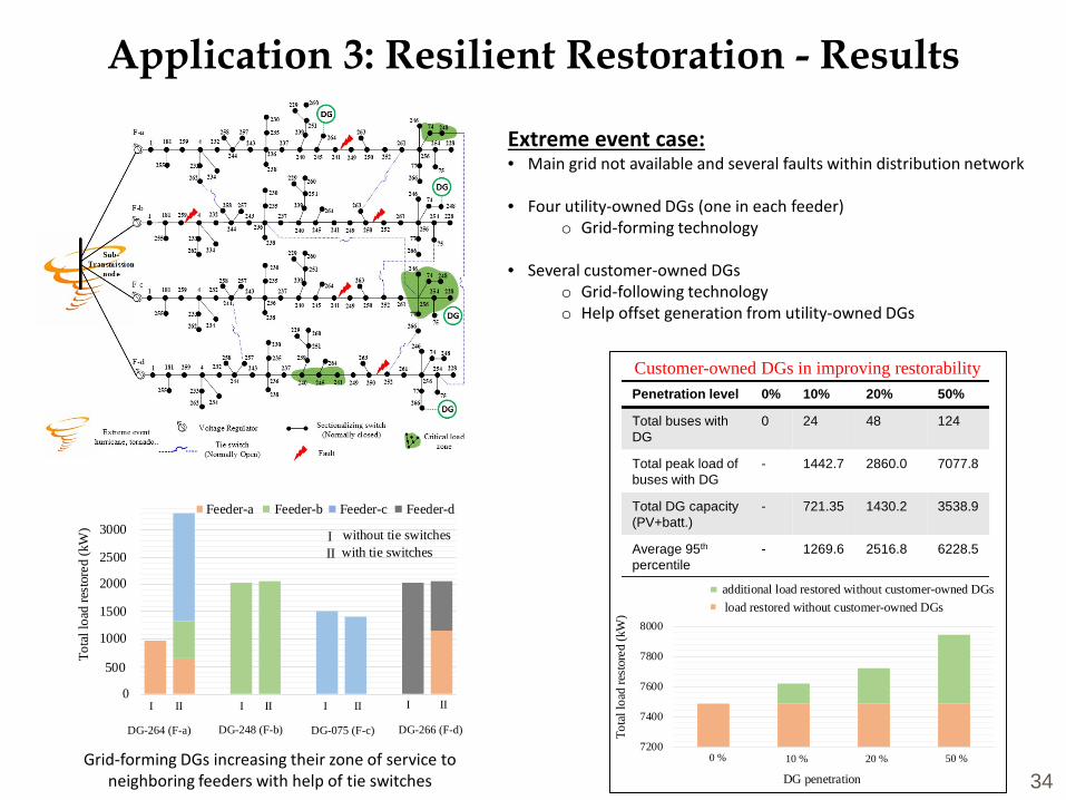
Application 3: Resilient Restoration - Results

0

500

1000

1500

2000

2500

3000

1 2 3 4 5 6 7 8 9 10 11

Tota

l loa

d re

stor

ed (k

W)

Feeder-a Feeder-b Feeder-c Feeder-d

DG-264 (F-a) DG-248 (F-b) DG-075 (F-c) DG-266 (F-d)

III

without tie switcheswith tie switches

I II I II I II I II

500

1000

1500

2000

2500

3000

7200

7400

7600

7800

8000

1 2 3 4

additional load restored with customer-owned DERsload restored without customer-owned DERs

DG penetration

Tota

l loa

d re

stor

ed (k

W)

0 % 10 % 20 % 50 %

load restored without customer-owned DGsadditional load restored without customer-owned DGs

Penetration level 0% 10% 20% 50%

Total buses with DG

0 24 48 124

Total peak load of buses with DG

- 1442.7 2860.0 7077.8

Total DG capacity (PV+batt.)

- 721.35 1430.2 3538.9

Average 95th

percentile- 1269.6 2516.8 6228.5

Customer-owned DGs in improving restorability

Extreme event case:• Main grid not available and several faults within distribution network

• Four utility-owned DGs (one in each feeder) o Grid-forming technology

• Several customer-owned DGso Grid-following technologyo Help offset generation from utility-owned DGs

Grid-forming DGs increasing their zone of service to neighboring feeders with help of tie switches

Demonstration using GridAPPS-D Platform

35

• GridAPPS-D - an open-source, standards based ADMS application development platformo Developed for the U.S. Department of Energy’s Advanced Distribution Management System

(ADMS) Program by the Grid Modernization Laboratory Consortium project GM0063 o Provides a method for developers to run their new applications on a real-time simulator with

extensive modeling and tool support.

R. Melton, K. P. Schneider, E. Lightner, T. McDermott, P. Sharma, Y.C. Zhang, F. Ding, S. Vadari, R. Podmore, A. Dubey, R. Weis, and E. Stephan, “Leveraging Standards to Create an Open Platform for the Development of Advanced Distribution Applications,” IEEE Access, vol. 6, pp. 37361-37370, June, 2018

SCADA/DMSMeasurements

AMI DataSmart Meter Data

DERMS/MGMSData

GOSS/FNCS Message Bus

OMS Data

Distribution System Simulator

python

Distribution Systems Restoration with DERs

Fault Location

SSW StatusLCS StatusDER Control Switch

Visualization

GridAPPS-D

DERs ParameterSwitch StatusLoad Parameters

Future Research Directions

36

Large-scale engineered systems with time and space fragmented control and an increased level of variability and uncertainty from DERs

• Challenging to solve operational problem for a large-scale optimization problem (mostly non-convex and with mixed-integer) in a stochastic setting for a three-phase unbalanced system.

Poor situational awareness due to limited measurement and sensing devices and inaccurate or unknown physical system planning and operational model along with noisy and compromised heterogeneous measurements:

• Simultaneously handling measurement and model uncertainty and noisy and compromised measurements.

Challenges not addressed in this work


37

• For optimal distribution system operations, mostly model-based methods have also emerged in past few years.

A combination of data-driven and physics-based model that can learn probabilistic relationships within observed and unobserved variables using measurement set and physics-based models.

Why not simply learn optimal decision from measurements?

• Completely model-free methods have also been proposed for estimation, control, and optimization.

• However, these do not generalize well.


Further Information

38

• Website: https://eecs.wsu.edu/~adubey/index.html• Research Projects:

https://eecs.wsu.edu/~adubey/research.html• Publications: https://eecs.wsu.edu/~adubey/papers.html

Anamika DubeyEECS, Washington State University

[email protected]

https://eecs.wsu.edu/%7Eadubey/index.html

https://eecs.wsu.edu/%7Eadubey/research.html

https://eecs.wsu.edu/%7Eadubey/papers.html

mailto:[email protected]

Research Group

39

Anandini Gandluru Andrew Cannon

Advisor: Dr. Anamika Dubey

Left to Right: Shiva Poudel, Gayathri Krishnamoorthy, Rabayet Sadnan Rahul Jha, Mohammed Ostadijafari, Surendra Bajagain

40

Thank you

Washington State University

Anamika DubeyEECS, Washington State University

[email protected]

Sponsors:

Questions?

mailto:[email protected]

Additional Slides

41

Device Models

42

Voltage regulator

Capacitor banks DERs/Smart Inverters

Load model- Voltage dependent load model is derived

using the CVR factor

𝐶𝐶𝑉𝑉𝐶𝐶 =% 𝑟𝑟𝑒𝑒𝑑𝑑𝑢𝑢𝑐𝑐𝑠𝑠𝑚𝑚𝑒𝑒𝑚𝑚 𝑒𝑒𝑓𝑓 𝑃𝑃/𝑄𝑄% 𝑣𝑣𝑒𝑒𝑙𝑙𝑠𝑠𝑑𝑑𝑔𝑔𝑒𝑒 𝑟𝑟𝑒𝑒𝑑𝑑𝑢𝑢𝑐𝑐𝑠𝑠𝑚𝑚𝑒𝑒𝑚𝑚

𝒑𝒑𝑳𝑳𝒊𝒊𝒑𝒑 = 𝒑𝒑𝒊𝒊𝟎𝟎

𝒑𝒑 + 𝑪𝑪𝑪𝑪𝑹𝑹𝒑𝒑𝒑𝒑𝒊𝒊𝟎𝟎

𝒑𝒑

𝟐𝟐(𝒗𝒗𝒊𝒊

𝒑𝒑 − 𝑪𝑪𝟎𝟎𝟐𝟐)

𝒑𝒑𝑳𝑳𝒊𝒊𝒑𝒑 = 𝒑𝒑𝒊𝒊𝟎𝟎

𝒑𝒑 + 𝑪𝑪𝑪𝑪𝑹𝑹𝒑𝒑𝒑𝒑𝒊𝒊𝟎𝟎

𝒑𝒑

𝟐𝟐(𝒗𝒗𝒊𝒊

𝒑𝒑 − 𝑪𝑪𝟎𝟎𝟐𝟐)

CVR factor can be obtained using the ZIP model

• Reactive power support is constant𝑄𝑄𝑖𝑖 = 𝑢𝑢𝑖𝑖𝑣𝑣𝑖𝑖𝑄𝑄𝐶𝐶

where, 𝑢𝑢𝑖𝑖 ∈ 0,1 , status of capacitor bank at node i

• Reactive power support depends on ratingof DGs

Mathematically:taking , 𝑆𝑆𝑖𝑖 = 1.15 ∗ 𝑃𝑃𝑖𝑖,𝑟𝑟𝑎𝑎𝑟𝑟𝑒𝑒𝑟𝑟

𝑄𝑄𝑖𝑖 = ± 𝑆𝑆𝑖𝑖𝑗 − 𝑃𝑃𝑖𝑖𝑗

𝑄𝑄𝑖𝑖 is the control variable for the optimization

A 32-step voltage regulator:𝑉𝑉𝑗𝑗𝑝𝑝 = 𝑉𝑉𝑖𝑖

𝑝𝑝 = 𝑑𝑑𝑝𝑝𝑉𝑉𝑖𝑖𝑝𝑝, 𝐼𝐼𝑖𝑖𝑖𝑖𝑖

𝑝𝑝 = 𝑑𝑑𝑝𝑝𝐼𝐼𝑖𝑖′𝑗𝑗𝑝𝑝

𝑑𝑑𝑝𝑝 = ∑𝑗𝑗=13𝑗 𝑏𝑏𝑗𝑗𝑥𝑥𝑗𝑗 𝐴𝐴𝑝𝑝= 𝑑𝑑𝑝𝑝𝑗

𝑣𝑣𝑗𝑗𝑝𝑝 = 𝐴𝐴𝑝𝑝𝑣𝑣𝑖𝑖

𝑝𝑝 (𝑣𝑣𝑖𝑖𝑝𝑝 = 𝑉𝑉𝑗𝑗

𝑝𝑝2)

𝐴𝐴𝑝𝑝 = ∑𝑗𝑗=13𝑗 𝑏𝑏𝑗𝑗𝑗𝑥𝑥𝑗𝑗 (𝑥𝑥𝑗𝑗 ∈ 0,1 )∑𝑗𝑗=13𝑗 𝑥𝑥𝑗𝑗 = 1 (Voltage Regulator tap position)where, 𝑏𝑏𝑗𝑗 ∈ {0.9, 0.92, … … … 1.1}

Power Flow with Switch Model

43

�𝑖𝑖→𝑗𝑗∈𝐷𝐷

𝛿𝛿𝑖𝑖𝑗𝑗𝑷𝑷𝑖𝑖𝑗𝑗 = 𝑠𝑠𝑗𝑗𝑷𝑷𝑳𝑳𝒊𝒊 + �𝑗𝑗→𝑐𝑐 ∈𝐷𝐷𝑖𝑖≠𝑐𝑐

𝛿𝛿𝑗𝑗𝑐𝑐𝑷𝑷𝒊𝒊𝒋𝒋 �𝑖𝑖→𝑗𝑗∈𝐷𝐷

𝛿𝛿𝑖𝑖𝑗𝑗𝑸𝑸𝑖𝑖𝑗𝑗 = 𝑠𝑠𝑗𝑗𝑸𝑸𝑳𝑳𝒊𝒊 + �𝑗𝑗→𝑐𝑐 ∈𝐷𝐷𝑖𝑖≠𝑐𝑐

𝛿𝛿𝑗𝑗𝑐𝑐𝑸𝑸𝒊𝒊𝒋𝒋

𝛿𝛿𝑖𝑖𝑗𝑗 𝑼𝑼𝑖𝑖 − 𝑼𝑼𝑗𝑗 = 2 �𝒓𝒓𝑖𝑖𝑗𝑗𝑷𝑷𝑖𝑖𝑗𝑗 + �𝒙𝒙𝑖𝑖𝑗𝑗𝑸𝑸𝑖𝑖𝑗𝑗

• Linear real and reactive power flow function of switch status

• Switch open or close status decides which radial configuration to operateo Power flow in open switch = 0o Voltage drop equations along the closed switch only

Sub station

Closed

Open

𝑷𝑷47 = 𝑸𝑸47 = 0

𝑼𝑼7 = ℱ (𝑼𝑼6,𝑷𝑷67,𝑸𝑸67, �𝒓𝒓67, �𝒙𝒙67)

𝑇𝑇𝑟𝑟𝑒𝑒𝑒𝑒 1

Sub station

Closed

Open

𝑷𝑷67 = 𝑸𝑸67 = 0

𝑼𝑼7 = ℱ (𝑼𝑼4,𝑷𝑷47,𝑸𝑸47, �𝒓𝒓47, �𝒙𝒙47)

𝑇𝑇𝑟𝑟𝑒𝑒𝑒𝑒 2

44

Integration with PNNL’s GridAPPS-D Platform:Restoration of Power Distribution Network

Fault isolation and restoration

Integration in Platform

IEEE 123-bus test case

IEEE 123-bus test case simulated in Platform

Network-level Optimization for Unbalanced Power Distribution … · Challenges: Network-level...

Documents

Transcript of Network-level Optimization for Unbalanced Power Distribution … · Challenges: Network-level...