NBER WORKING PAPER SERIES

MERGERS AS REALLOCATION

Boyan JovanovicPeter L. Rousseau

Working Paper 9279http://www.nber.org/papers/w9279

NATIONAL BUREAU OF ECONOMIC RESEARCH1050 Massachusetts Avenue

Cambridge, MA 02138October 2002

We thank the NSF for support, A. Faria, R. Lucas, R. Shimer and N. Stokey for useful comments, and TanyaColmant-Donabedian for help with obtaining some of the early data on mergers. The views expressed hereinare those of the authors and do not necessarily reflect the views of the National Bureau of EconomicResearch.

© 2002 by Boyan Jovanovic and Peter L. Rousseau. All rights reserved. Short sections of text, not to exceedtwo paragraphs, may be quoted without explicit permission provided that full credit, including © notice, isgiven to the source.

Mergers as ReallocationBoyan Jovanovic and Peter L. RousseauNBER Working Paper No. 9279October 2002JEL No. O3, L2, N8

ABSTRACT

We argue that takeovers have played a major role in speeding up the diffusion of newtechnology. The role that they play is similar to that of entry and exit of firms. We focus on andcompare two periods: 1890-1930 during which electricity and the internal combustion engine spreadthrough the U.S. economy, and 1971-2001 . the Information Age.

Boyan Jovanovic Peter L. RousseauDepartment of Economics Department of EconomicsNew York University Vanderbilt University269 Mercer St. Box 6182, Station BNew York, NY 10002 Nashville, TN 37235and NBER and NBERbj2@nyu.edu peter.l.rousseau@vanderbilt.edu

Mergers as Reallocation

Boyan Jovanovic and Peter L. Rousseau∗

October 2002

Abstract

We argue that takeovers have played a major role in speeding up the dif-fusion of new technology. The role that they play is similar to that of entryand exit of Þrms. We focus on and compare two periods: 1890-1930 duringwhich electricity and the internal combustion engine spread through the U.S.economy, and 1971-2001 � the Information Age.

1 IntroductionIt has been said that new technology replaces and therefore �destroys� old technology.But if we think further about the process by which this replacement takes place,it becomes clear that much of �creative destruction� would more aptly be namedreallocation. In trying to adopt a new technology, a Þrm may re-train some of itsworkers and replace others, and it can re-Þt its buildings and equipment, wherepossible, and replace the rest. If it fails in the attempt to reorganize internally, theÞrm will probably disappear and its assets will be reorganized externally. In thatcase the Þrm will either liquidate, or it will be taken over. Either way, however, theexisting human and physical capital is no more likely to be �destroyed� than during anepisode of internal reorganization. It will simply change management. Indeed, a newtechnology cannot spread quickly economy-wide unless these reallocation mechanismswork smoothly. This paper studies these mechanisms.

We study and measure, in particular, the two external adjustment mechanisms� mergers and entry-and-exit (E&E) � using the stock-market capitalization of theÞrms involved. In Figure 1, the U-shaped top line is our estimate of the total amountof capital that has been reallocated on the U.S. stock market over the past 112years. Its components are the stock market capitalization of entering and exiting

∗NYU and the University of Chicago, and Vanderbilt University. We thank the NSF for support,A. Faria, R. Lucas, R. Shimer and N. Stokey for useful comments, and Tanya Colmant-Donabedianfor help with obtaining some of the early data on mergers.

1

1890 '00 '10 '20 '30 '40 '50 '60 '70 '80 '90 2000

Target value

(left scale)(Entry+Exit)/2

(right scale)

0

3

6

0

6

12

(right scale)Total reallocation

�Monopolization� Wave

�Scale Economies� �Hubris� �Decade of �Global� Wave Wave Greed� Wave Wave

0

6

12

Figure 1: Reallocated capital and components as percentages of stock market value,with merger waves shaded, 1890-2001.

Þrms divided by two, and the value of merger targets.1 E&E, given by the center

1We identify targets for 1926-2001 using the stock Þles distributed by the University of Chicago�sCenter for Research on Securities Prices (CRSP) and various supplementary sources. We use work-sheets for the manufacturing and mining sectors that underlie Nelson (1959) for 1890-1930. Thetarget series includes the market values of exchange-listed Þrms in the year prior to their acquisi-tion, and reßects 9,030 mergers. Stock market capitalizations after 1925 are from CRSP. Prior tothat they are from our extension of CRSP backward through 1885 using contemporary newspapers.Entries and exits are also drawn from CRSP and our newspaper sources. Before assigning a Þrmas an �exit� we check the list of hostile takeovers from Schwert (2000) for 1975-1996 and individualissues of theWall Street Journal from 1997-2001 to ensure that we record Þrms taken private undera hostile tender offers as mergers. See footnotes 1 and 4 of Jovanovic and Rousseau (2001) for adetailed description of these data and their sources.

2

line, is a rough measure of how much capital exits from the stock market and comesback in under different ownership, or at least under a different name. The lower lineis the stock-market value of merger targets.

The bottom panel shows the Þve merger waves and at the very top we list thenames most commonly given to these waves.2 This paper will argue, however, thatthe Þrst two waves represent a form of external reallocation of resources in response tothe simultaneous arrival of two general purpose technologies (GPTs) � electricity and(to a lesser extent) internal combustion � and that the last two represent reallocationin response to the arrival of the microcomputer and information technology (IT). Themiddle �Managerial Hubris� wave was composed mainly of conglomerate mergers anddoes not seem to Þt our story. Two speciÞc points emerge in Figure 1:

1. Each merger wave was accompanied by a rise in E&E. The deviations fromtrend are positively related � the correlation is 0.46.

2. Total reallocation has no signiÞcant trend, but mergers have grown relative toE&E � the ratio rises by a factor of 9, from 0.18 in the 1890�s to 1.63 in the1990�s.

Fact 1 arises, we argue, because society will use both margins of external adjust-ment in response to a technological shock. Fact 2 arises, we believe, because of theincreased importance of teamwork and organization capital which also has causedmarket values of companies to rise relative to their book values.

Our contrast of two periods of major technological change � electriÞcation (1890-1930) and IT (1970-2002) is in the spirit of David (1991).

2 ModelFirst we describe a standard one-technology �Ak� model; we then add a secondtechnology with its own capital that suddenly and unexpectedly becomes available.

2.1 One-technology model

Preferences are1

1− σZ ∞

0

e−ρtc1−σt dt,

aggregate output isy = zk,

2We deÞne the shaded merger �waves� as starting when the series for target value stays above atightly-speciÞed HP trend (λ=100 in the RATS Þlter program) for two or more consecutive years.The wave �ends� when the series falls below trend for two consecutive years.

3

capital evolves asúk = −δk + x,

and the income identity isy = c+ x.

Equating the marginal product of capital, z, to the user cost of capital, r + δ, andsubstituting into the consumer�s Þrst-order conditions for optimal consumption úc/c =(r − ρ) /σ gives us the constant-growth-rates of income and consumption

úy

y=úc

c=z − δ − ρ

σ.

This model has no transitional dynamics because it has a single state variable, k.

2.2 A second technology arrives

Starting from a state in which all its capital embodies a technology z1, how does theeconomy transit to a state in which all its capital embodies technology z2? If thearrival of z2 at t = 0 was unexpected, the growth rate before the transition wouldhave been (z1 − δ − ρ) /σ, and after the transition is over at date T the growth ratewill be (z2 − δ − ρ) /σ. For the intervening T periods, two kinds of capital coexist,k1 and k2. This is the era of reallocation.

De novo investment and upgrading New capital can be produced from theconsumption good, or from old capital.De novo entry of k2.�As is usual in one-sector growth models, the production

function for new capital (not counting depreciation) is

úk2 = x2 (1)

where x2 is the consumption foregone for the purpose of creating k2.Two technologies for converting k1 into k2 or into c.�We shall model these up-

grading costs as convex costs of adjustment. We assume two distinct upgradingactivities, one of which involves only k1 while the other requires both k1 and k2. Theintuition is easiest if we imagine that k1 and k2 must reside in different Þrms � callthese z1-Þrms and z2-Þrms

1. Conversion via �Exit�. Let ∆1 be amount of k1 that the z1-Þrms retire andconvert into an equal number, ∆1, of units of the consumption good. In sodoing, they forego

ψ

µ∆1k1

¶k1

units of output. Assume that ψ is increasing, convex and differentiable withψ0 (0) = 0. This adjustment cost is homogeneous of degree 1 in (∆1, k1).

4

2. Conversion via �Acquisition�. Let ∆2 be the total amount of k1 that the z2-Þrms acquire from z1-Þrms and convert into ∆2 units of k2. In so doing, theyforego

φ

µ∆2

k2

¶k2

units of output. Assume that φ is increasing, convex and differentiable withφ0 (0) = 0. This adjustment cost is homogeneous of degree 1 in (∆2, k2).

Output and the evolution of k1 and k2. During the transition, t ∈ [0, T ], bothk1 and k2 are used. Net of upgrading costs, output is

y = (z1 − ψ [ε]) k1 + (z2 − φ [m]) k2, (2)

where

ε ≡ ∆1

k1

is the exit rate of k1, and

m =∆2k2

is the acquisitions rate relative to k2. Consumption is

c = y − x1 − x2.

The two capital stocks evolve as follows:

úk1 = −δk1 + x1 − (εk1 +mk2) (3)úk2 = −δk2 + x2 + εk1 +mk2 (4)

These two laws of motion are standard but for the reallocation term εk1+mk2, whichis subtracted from the right-hand side of (3) and added back in (4).

2.3 Equilibrium

Equilibrium consists of m, ε, x1and x2 such that Þrms maximize and such that therepresentative agent consumes optimally. The initial conditions are k1,0 = 1, k2,0 =0, and the aggregate laws of motion (3) and (4) hold with the added restrictionthat k1,t ≥ 0. The model has neither external effects nor monopoly power and theAppendix uses the planner�s problem to derive the equilibrium formally. In thissection we shall give the market-economy interpretation.

Upgrading.�Let q be the price of k1, and Q the price of k2. Optimal upgradingby z1-Þrms implies that

ψ0 (ε) = Q− q. (5)

5

and optimal upgrading by z2-Þrms implies that

φ0 (m) = Q− q. (6)

In both cases the replacement cost for k1 is q, and the upgraded capital has a priceof Q. The difference between the two is equated, in (6) and (5) to the marginal costof adjustment.3

Investment.�We assume that x2 > 0. Then

Q = 1.

On the other hand, it will turn out that q < 1 for all t ∈ [t, T ), and therefore x1 = 0throughout the transition.

Output and upgrading rents.� k1 and k2 play a dual role here. Each producesoutput, and each assists in the upgrading process. Upgrading is subject to increasingmarginal costs and so, in equilibrium, entails a rent. The per-unit upgrading rentthat k1 draws is

πε (q) ≡ maxε{ε− (qε+ ψ [ε])} ,

and the per-unit rent that k2 draws is

πm (q) ≡ maxm{m− (qm+ φ [m])} .

Consumption growth during the transition is

úc

c=1

σ(z2 + π

m (q)− ρ− δ) (7)

and the rate of interest isr = z2 − δ + πm (q) .

Output in (2) rises monotonically because, by (5) and (6), ε and m both declinemonotonically. This is driven by the monotonic rise in q that we are about to show.

The monotonic rise in q during the transition If we can solve for q, we shallbe able to infer ε, m, πε (q), πm (q), úc/c, and r. The price of k1 must be such thatthe marginal product of k1 equals its user cost:

z1 + πε (q) = (r − δ) q − úq.

Since úQ = 0, the corresponding condition for k2 is

z2 + πm (q) = r − δ.

3In our partial-equilibrium treatment of takeovers as an investment (Jovanovic and Rousseau2002), the equivalent of (6) is eq. (8). That paper also assumes adjustment costs on x which wehave suppressed here in order to keep the analysis manageable.

6

Combining these two conditions and eliminating r we are left with4

úq

q= z2 + π

m (q)− (z1 + πε [q])

q. (8)

Let q∗ be the largest value of q at which

z2 + πm (q) =

(z1 + πε [q])

q

for all t ∈ [0, T ]. Since πm (q) = πε (q) = 0 when q ≥ 1, we have 0 < q∗ < 1. Thisrest-point q∗ is unstable from above:

q > q∗ =⇒ úq > 0.

But q must approach unity at t → T because as of date T , k1,t becomes zero and εtand mt must both become zero. That is, since φ

0 (0) = 0, a unit of k1 is at date T asvaluable as a unit of k2 because it can be upgraded costlessly. It must therefore bethat

q0 ∈ (q∗, 1) and qT = 1and, from (8), that úq > 0 all through the transition, . Finally, úqT = z2 − z1. Figure 2illustrates the solution for qt.

2.4 Summary of implications

The qualitative implications are as follows:

1. At t = 0, output falls from z1k1 to (z1 − ψ [ε0]) k1 and then starts to rise mono-tonically.

2. The value of capital also falls from 1 to q0. Wealth falls from k1,0 to q0k1,0.

3. Thereafter, qt rises monotonically to 1, and k1 falls monotonically to zero atdate T , as do ε and m.

4. Total exits, qεk1, decline monotonically, whereas total acquisitions, qmk2 startand end at zero and are, essentially, inverted U-shaped during the transition.

5. The rate of interest jumps from z1 − δ to z2 − δ + πm (q0) and then declinesmonotonically to z2 − δ where it remains thereafter.

6. Consumption falls at date zero. After that consumption growth declines mono-tonically. More precisely,

gc =

z1−δ−ρ

σfor t < 0

z2+πm(qt)−δ−ρσ

for t ∈ (0, T )z2−δ−ρ

σfor t ≥ T.

4This equation is derived for the planner�s shadow price of k1 in (17) of the Appendix.

7

t T

q

q0

0

1

Slope = z2 - z1

qt

q*

Figure 2: The solution for qt.

2.5 Simulations

We now simulate the model. We assume that σ = 1 and that adjustment costs arequadratic:

φ (m) =m2

2µand ψ (ε) =

ε2

2ν. (9)

The date-0 initial conditions are

k1 = 1 and k2 = 0

and the other boundary conditions are

k1,T = 0, (10)

andqT = 1. (11)

8

Finally, because the shock is unforeseen, the present value of consumption as of datezero (just after the shock) equals wealth, which is just q0k1,0. Since k1,0 ≡ 1, the lastcondition is

q0 =

Z T

0

exp

µZ t

0

rsds

¶ctdt+ e

−rT cTρ. (12)

Parameter choices are reported in Figures 3 and 4. If we assume that discounting isat a rate of Þve percent per year, the value of ρ = 0.10 determines the period-lengthat 2 years. In both of the simulations we have assumed that the new technologydoubles the rate of growth from z1 − ρ = 0.015, or three-quarters of a percent peryear before the transition, to z2−ρ = 0.03, or 1.5 percent per year after the transition.The adjustment-cost parameters, µ and ν, are set much higher implying a far smalleradjustment cost than the micro evidence (see below) suggests. Our main interest isin how the diffusion of the new technology is implemented. The three ways in whichk2/k1 grows are:

1. Acquisitions. Relative to market capitalization, acquisitions are

M =qmk2k2 + qk1

. (13)

2. Exits. Relative to market capitalization, exit is

E =qεk1

k2 + qk1, (14)

and E must decline on average from ε at t = 0 to zero at date T .

3. De novo investment.X =

x2k2 + qkt

These three series are plotted in the upper left panels of Figures 3 and 4. Duringthe electricity period, exits were several times as important as acquisitions, and thisis the main fact that we obtain in Simulation 1 (Figure 3), along with a transitionthat lasts 32 years. If teamwork and organization capital have indeed become moreimportant and the cost of destroying them has risen, this implies a fall in ν. Simulation2 (Figure 4) raises the ratio µ/ν by a factor of 10, and although it achieves the neededsubstitution of acquisitions for exits, the transition still takes 32 years.

Simulation 1 shows k2 overtaking k1 after 10 years (i.e., 5 periods). When weraise the adjustment costs in simulation 2, Figure 4 shows that overtaking does notoccur until the 17th year. Since, in Simulation 2, φ and ψ are much higher thanin Simulation 1, it is surprising that we do not see more substitution towards X.Exits lead acquisitions in both simulations. Finally in the last panel we plot the newproductivity relative to old trend and Þnd that the productivity slowdown lasts about7 years in both simulations.

9

10

Period0 2 4 6 8 10 12 14 16

0

4

8

12

16

20

Mergers (M)

Investment (X)

Exits (E)

Period0 2 4 6 8 10 12 14 16

0

0.2

0.4

0.6

0.8

1

1.2

�Old� capital (k1)

�New� capital (k2)

Period0 2 4 6 8 10 12 14 16

0.92

0.94

0.96

0.98

1

qt sequence

Period0 2 4 6 8 10 12 14 16

0.9

0.95

1

1.05

1.1

1.15

1.2

1.25

Output relative to old trend

Model settings:

z1 = 0.115, z2 = 0.130, µ = 2.7, ν = 2.7, ρ = 0.1, σ = 1, δ = 0.

Figure 3. Transitional dynamics for �Electricity� model.

11

Period0 2 4 6 8 10 12 14 16

0

4

8

12

16

20

Mergers (M)

Investment (X)

Exits (E)

Period0 2 4 6 8 10 12 14 16

0

0.2

0.4

0.6

0.8

1

1.2

�Old� capital (k1)

�New� capital (k2)

Period0 2 4 6 8 10 12 14 16

0.92

0.94

0.96

0.98

1

qt sequence

Period0 2 4 6 8 10 12 14 16

0.9

0.95

1

1.05

1.1

1.15

1.2

1.25

Output relative to old trend

Model settings: z1 = 0.115, z2 = 0.130, µ = 0.60, ν = 0.06, ρ = 0.1, σ = 1, δ = 0.

Figure 4. Transitional dynamics for �IT� model.

1970 1975 1980 1985 1990 1995 20000

10

20

30

40

4

6

8

10

12

used capital purchases

acquisitions(left scale)

(right scale)

correlation=.44

Figure 5: Used and Acquired Capital as Percentages of Total Investment, 1971-2001

3 EvidenceWe begin with our assumption that the transition is technological and that takeoversand exits are reallocative. First, we know from McGuckin and Ngyen (1995) andSchoar (2000) that the productivity of acquiring Þrms� plants falls and that the pro-ductivity of the targets� plants rises following a takeover. Also, Lichtenberg and Siegel(1987) Þnd that plants changing owners had lower initial levels of productivity andhigher subsequent productivity growth than plants that did not change hands. TheseÞndings support our assumption that a takeover implies that k1 is transformed intothe more productive k2, and that the acquirer faces an adjustment cost.

Second, the trading of used capital is correlated with mergers.

Our model treats M&As like purchases of used capital at the price of q. In fact,trading in the two kinds of used capital � bundled and disassembled � has movedtogether over the last thirty years. Figure 5 shows this fact. It plots acquired capitaland direct purchases of used capital among exchange-listed Þrms as percentages oftheir annual investment from 1971 to 2001. We derive the series using all Þrms

12

common to CRSP and Standard and Poor�s Compustat.5 The two series do notoverlap in coverage, and thus if we add them, we have the fraction of investmentspent on used capital. The correlation coefficient between the two series is 0.44.

3.0.1 Acquisitions and sectoral exposure to GPTs

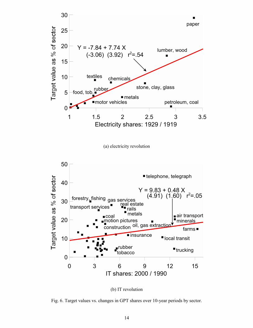
If 1890-1930 and 1970-2002 are technological transitions, then we should have seenmore upgrading and reallocation in the sectors that were absorbing more of the twoGPT�s. Figure 6 reports, for each epoch, a measure of sectoral absorption of thetwo GPTs at the tail end of the two episodes. The Þgures are comparable, and areconstrained by the sectoral investment data that we could Þnd for the Þrst epoch.6

The acquisitions that we report are for 1925-30 and 1997-2000 (the waves as deÞnedin Figure 1).7 That is, we look at the growth of the GPT shares over the 10-yearperiods and then report acquisitions during the end-of-period wave.The relation is positive in both epochs, but more so for the electriÞcation era.

The correlation coefficients are 0.74 and 0.22 respectively.

3.0.2 Acquisitions, exits and IPOs by sector

If m and ε are performing the same sort of reallocative function, then they should bepositively correlated over sectors. It turns out that they are. The rank correlationsbetween IPOs and exits on the one hand and acquisitions on the other, with ranksbased upon the percentage of each in total sector value (with the merger samples asdeÞned in fn. 7) are given below.

Period rank correlation signiÞcance # of sectorsMergers and IPOs

1925-1930 0.718 1% 151997-2000 0.227 10% 53

Mergers and Exits1925-1930 0.343 10% 151997-2000 0.123 NS 53

Once again, the electricity era seems to Þt the model better.5Capital sales include property, plant, and equipment (Compustat item 107). Acquisitions include

funds used for and costs related to the purchase of another company in the current year or anacquisition in a prior year that was carried over to the current year (item 129). Investment is thesum of acquired capital (item 129) and direct capital expenditures (item 128). We compute theratios in Figure 5 after summing each data item across active Þrms in each year.

6The sectors and electricity shares shown in the upper panel of Figure 6 are from David (1991).7A good deal of U.S. merger activity took place outside of the stock exchange over the 1890-1930

period, and a sectoral breakdown would not be possible unless we use these off-exchange transactions.Panel (a) of Figure 6 therefore uses all targets and sector designations recorded in the worksheetsunderlying Nelson (1959), and then divides by the total value of exchange-listed Þrms belonging toa given sector to form the vertical axis quantities. Panel (b) of Figure 6 reßects activity amongexchange-listed Þrms only.

13

14

Electricity shares: 1929 / 19191 1.5 2 2.5 3 3.5

0

5

10

15

20

25

30

Y = -7.84 + 7.74 X

paper

lumber, wood

stone, clay, glass

petroleum, coalmetals

chemicalstextiles

rubber

motor vehicles

food, tob.

(-3.06) (3.92) r2=.54

IT shares: 2000 / 19900 3 6 9 12 15

0

10

20

30

40

50

Y = 9.83 + 0.48 X

telephone, telegraph

forestry, fishing gas services

trucking

farmsmineralsair transport

local transit

oil, gas extraction

metalsrails

real estate

insurance

transport services

construction

rubbertobacco

coalmotion pictures

(4.91) (1.60) r2=.05

(a) electricity revolution

(b) IT revolution

Fig. 6. Target values vs. changes in GPT shares over 10-year periods by sector.

3.0.3 Acquisitions and exits over time

Now we compare the simulations with the aggregate data. In the upper left panels ofFigures 3 and 4 we simulatedM , E, and X, and now we look at their actual behavior.Figure 7 is the empirical counterpart.

Acquisitions should be inverted-U in that a merger wave must begin and end atzero. Figure 7 shows that mergers crest during the second half of each transition.

Since k1 is decreasing, total exits should fall over the transition. Figure 7 showsthat exits have a slight negative trend, though the T-statistics in a regressions of exitson trend are only 1.27 for the electricity era and 0.90 for the IT era.

We also simulated X in Figures 3 and 4, but in practice we do not know theinvestment for Þrms that actually traded on the stock market. For the economy asa whole, investment net of residential structures averaged 10.5% of GDP for 1890-1930 and 11.5% for 1970-2001.8 Of course, these shares are much higher than in oursimulations, but the units are not the same. If the aggregate capital stock was aboutthree times nominal output from 1890-1930 and about two and a half times outputfrom 1970-2001, we can divide each average by these multiples to express investmentas shares of stock market capitalization, assuming of course that listed Þrms form theircapital stocks in the same way as unlisted ones. The resulting investment shares of3.5% for 1890-1930 and 4.6% for 1970-2001 are much closer to the simulations. Panel(b) of Figure 7 shows the upward trend in investment that the model predicts for thetransitions, but panel (a) does not.

3.0.4 A rising q

Using the average market-to-book ratios of exiting and target Þrms as a proxy for q,panel (a) of Figure 8 shows that q has been rising during the IT episode. But so hasQ when measured as the average market-to-book values of acquirers, and this ßatlycontradicts the implication that Q = 1.9 The model could explain values of Q in

8We obtain private domestic Þxed investment and its price deßator for 1970-2001 from the August2002 issue of the Survey of Current Business (Table 1, pp. 123-4, and Table 3, pp. 135-6) and excludenon-farm residential investment. We use Kendrick (1961, Table A-IIa, column 7) for 1890-1930, andthen subtract residential nonfarm construction from worksheets underlying Kuznets (1961, TableT-11).

9We use the Compustat Þles to compute Þrm q�s, and deÞne market value as the sum of commonequity at current share prices (the product of items 24 and 25), the book value of preferred stock(item 130), and short- and long-term debt (items 34 and 9). Book values are computed similarly,but use the book value of common equity (item 60) rather than the market value.

Since the company coverage within Compustat is very thin before 1972, we begin to computeQ�s at this time. We count Þrms that disappear from Compustat as targets or exits, but only if theÞrm has been on the Þles for at least two years. Thus, the series for q̄ and q̄/Q begin in 1974. Weomitted q�s for Þrms with negative values for net common equity from the plot since they implynegative market to book ratios, and eliminated observations with market-to-book values in excessof 100, since many of these were likely to be serious data errors.

15

16

1970 1975 1980 1985 1990 1995 20000

0.1

0.2

0.3

0.4

0.5

0.6

0

1

2

3

4

5

6Mergers (M)

(left scale)

(right scale)

Exits (E)

(right scale)Investment (X)

1890 1895 1900 1905 1910 1915 1920 1925 19300

1

2

3

4

5

Mergers (M)

Exits (E)

Investment (X)

Year 1970 1975 1980 1985 1990 1995 20001

1.5

2

2.5

3

3.5

Q

q

_

_

Year 1970 1975 1980 1985 1990 1995 2000

0.6

0.7

0.8

0.9

1

1.1

Qq /__

(a) electricity revolution (b) IT revolution

Figure 7. The values of exiting firms and merger targets in two technological epochs.

(a) Q�s by investment subgroup (b) the ratio of exiting and target firm q�s to acquirer Q�s

Figure 8. Prices of the two types of capital in the IT transition.

excess of unity if x2 also imposed convex adjustment costs on the Þrm, but the algebraloses its simplicity and results are hard to prove. Moreover, a part of the rise in bothq and Q may be due to the rising importance of unmeasured components of k2 whichare not on the Þrms� books. It is better, therefore, to concentrate on the ratio q/Q.In the theory, Q is unity and so

q =q

Q.

The theory predicts a monotonic rise in this ratio. Panel (b) of Figure 8 shows thatthe ratio has indeed risen, but much faster than the simulations in the third panel ofFigure 4.

4 Other evidence and puzzlesIn this section we report other, less favorable evidence, and other material that issomehow incongruous with the model and the logic.

4.0.5 The secular rise of acquisitions relative to exit and entry

Figure 1 shows a nine-fold increase in the ratio of acquisitions to E&E. We do notexplain the trend here, but we can re-formulate the puzzle in terms of our two adjust-ment costs. Assume they are quadratic as in (9). Then (6) and (5) readm = µ (1− q)and ε = ν (1− q) . Note that

m

ε=µ

ν.

If, for some reason, the ratio ν/µ were to fall, ε would fall relative to m. The nine-fold rise in the ratio of mergers to E&E over the past century suggests that the ratioµ/ν has risen by an order of magnitude over this period (which is also the differencebetween the Þrst and the second simulations in Figures 3 and 4). �Team capital� or�organization capital� may today be more important than it was in 1900, and thismakes it worthwhile to preserve the healthy parts of an underperforming Þrm and Þxonly the part that works poorly. If a Þrm is taken over, its teams and its organizationcan remain intact, whereas if it were to exit through bankruptcy its assets and peoplewill disperse, and this will destroy its team-speciÞc capital.

4.0.6 The stock-market drop

Initial stock-market capitalization is k1. Right after the shock, it falls to qk1. Withk1 = 1,the stock market thus exhibits an immediate drop at t = 0, from 1 to q.10

Figure 9 shows that the stock market declined in 1973-74. No such sudden drop is

10The drop is in this model due entirely to the jump in r. Hobijn and Jovanovic (2001) get abigger stock-market drop by assuming that the output produced by the old capital falls in pricewhen new capital is introduced � i.e., through the obsolescence of old capital.

17

Years 5 10 15 20 25 30 35 40

0

1

2

3

4

19001910

1920

1930

19801990

2001

1890/1970

Figure 9: The real Cowles/S&P stock price index across the the transition periods,1890-1931 and 1970-2001.

visible for stock prices in the early 1890�s. Why not? Maybe because the marketwas thin and unrepresentative in those days, with railway stocks absorbing a largechunk of market capitalization. More likely, the realization that the new technologywould work well was more gradual and was not prompted by any single event like thecompletion of the Niagara Falls dam in 1894.11

4.0.7 The productivity slowdown and multiple waves

The productivity slowdown (about 7 years) that the model seems to predict in thelast panels of Figures 3 and 4 is shorter than observed during the second transition,at least. This may be related to the bigger puzzle for this paper, namely that eachtechnological transition as we have deÞned it had two merger waves, and not justone, as the simulations imply.

11We obtain the composite stock price index from Wilson and Jones (2002), and deßate using theCPI.

18

4.0.8 Micro-estimates of φ and ψ

The two sets values for (µ, ν) of (2.7, 2.7) and (0.6, 0.06) used in the simulations arehigher than the micro data would suggest. In other words, the estimates that weare about to report from the micro data suggest much higher costs of adjustment(at least for acquisitions) than are needed to explain the aggregate data on exits andmergers.

In another paper we use Q-theory to derive an investment equation for acquisitionsfrom which one can uncover the adjustment-cost parameter. If φ (m) = m2

2µ, (6) reads

m = µ (Q− q). Table 1 of Jovanovic and Rousseau (2002) reports an estimate ofµ = 0.022 from the Compustat data. The estimate was divided by 100 in order toget it into the present units.

For the costs of exit we now look at evidence on the salvage value of capital fromRamey and Shapiro (2001). Consider the resources lost when a z1−Þrm retires someof its capital. Let pi be the sales price divided by the purchase price of machine i.Table 3 of Ramey and Shapiro reports the data. Per dollar spent on the machine, theÞrm�s cost of retiring machine i is Ci ≡ 1− pi. We imagine that if the Þrm were toretire some of its capital, it would Þrst sell off those machines for which pi was closestto unity, and so on in order of descending pi. Suppose the Þrm has k1 machines onhand, i = 1, 2, ....k1. Let G

³ik1

´be the cumulative distribution of Ci among the stock

of machines:

Ci = G

µi

k1

¶.

The total cost to the Þrm of retiring εk1 machines is

ψ (ε) k1 = k1

Z εk1

0

G

µs

k1

¶ds

= k1

Z ε

0

G (s0) ds0

after the change of variables s0 = s/k1, so that

ψ (ε) =

Z ε

0

G (s) ds.

Now suppose that the Ci are distributed uniformly on the interval [0, ν], so thatG (s) = 1

νs. Then ψ (ε) = ε2/2ν. The age-aggregated data underlying Figure 3 of

Ramey and Shapiro�s paper were kindly supplied us by Valerie Ramey, and we plotthem in Figure 10. Indeed, there are more Ci values close to unity than to zero.Ignoring this asymmetry, however, we would conclude that ν = 1.0, which actuallygives relatively low costs of adjustment, roughly half-way between the values of 0.06and 2.7 used in the simulations.

19

0 0.2 0.4 0.6 0.8 10

10

20

30

40

Figure 10: Frequency distribution of 1-pi from the Ramey and Shapiro (2001) data.

Finally, we have assumed that φ and ψ are both convex in spite of evidence tothe contrary. The micro data on acquisitions suggest a Þxed-cost component to φ,as we have argued in Jovanovic and Rousseau (2002). Similarly, exit is also likely toinvolve Þxed costs � e.g., the auction in Ramey and Shapiro (2001) was costly to setup. Such realism was sacriÞced in return for simpler algebra.

5 Related workWe mentioned David (1991) earlier. Boldrin and Levine (2001) also have a technologyfor converting old capital to new. Since they do not allow goods to be convertedinto new capital one for one, their results are different. In related theoretical work,Mortensen and Pissarides (1998) look at constant growth, not at transitions, and theyfocus on the labor market, but their work is similar in that they have two modes ofjob-improvement that are similar to the two that we have modeled. Caballero andHammour (1994) study transitions at business-cycle frequencies. Finally, Atkeson andKehoe (2001), Greenwood and Yorukoglu (1997) and Hornstein and Krusell (1996)study transitions, but they do not focus on adjustment costs like we do.

20

The argument that mergers reallocate resources in much the same way as E&Eimplies that they raise the values of the capital involved in mergers. Why, then, domerger announcements lead to declines in the prices of acquirer shares? Jovanovicand Braguinsky (2002) show that when Þrms have private information about thequality of the capital that they own, the bidder discount is consistent with takeoversbeing constrained efficient.

6 ConclusionThis paper has studied the role of acquisitions and E&E in two economy-wide techno-logical transformations. It reinforces the evidence in Jovanovic and Rousseau (2002)for the view that mergers reallocate capital to more productive purposes and to moreefficient managers. The adjustment costs associated with E&E seem to have risensubstantially relative to the adjustment costs associated with takeovers reßecting,probably, the rising importance of organization capital.

References[1] Atkeson, Andrew, and Patrick Kehoe. �The Transition to a New Economy Af-

ter the Second Industrial Revolution.� National Bureau of Economic Research(Cambridge, MA) Working Paper No. 8676, 2001.

[2] Bartel, Ann, and Nachum Sicherman. �Technological Change and the Skill Ac-quisition of Young Workers.� Journal of Labor Economics 16, no. 4 (October1998): 718-755.

[3] Boldrin, Michele, and David K. Levine. �Growth Cycles and market Crashes.�Journal of Economic Theory 96 (2001): 13-39.

[4] Boyd, John, and Edward C. Prescott. �Dynamic Coalitions: Engines of Growth.�American Economic Review 77, no. 2 (May 1987), Papers and Proceedings.

[5] Caballero, Ricardo J., and Mohamad L. Hammour. �The Cleansing Effect ofRecessions.� American Economic Review 84, no. 5 (December 1994): 1350-1368.

[6] David, Paul. �Computer and Dynamo: The Modern Productivity Paradox ina Not-Too-Distant Mirror.� In Technology and Productivity: The Challenge forEconomic Policy. Paris: OECD, 1991.

[7] Dow Jones Inc. The Wall Street Journal. 1997-2001, various issues.

[8] Hobijn, Bart, and Boyan Jovanovic. �The IT Revolution and the Stock Market:Evidence.� American Economic Review 91, no. 5 (December 2001): 1203-1220.

21

[9] Greenwood, Jeremy, and Mehmet Yorukoglu. �1974.� Carnegie-Rochester Con-ference Series 46 (June 1997): 49-95..

[10] Hornstein, Andreas, and Per Krusell. �Can Technology Improvements CauseProductivity Slowdowns?� NBER Macroeconomic Annual (1976): 209-259.

[11] Jovanovic, Boyan, and Peter L. Rousseau. �The Q-Theory of Mergers� AmericanEconomic Review 92, no. 2 (May 2002), Papers and Proceedings: 198-204.

[12] Jovanovic, Boyan, and Peter L. Rousseau. �Vintage Organization Capital.� Na-tional Bureau of Economic Research (Cambridge, MA) Working Paper No. 8166,March 2001.

[13] Jovanovic, Boyan, and Serguey Braguinsky. �Bidder Discounts and Target Pre-mia in Takeovers.� National Bureau of Economic Research (Cambridge, MA)Working Paper No. 9009, June 2002.

[14] Kendrick, John. Productivity Trends in the United States. Princeton: PrincetonUniversity Press, 1961.

[15] Kuznets, Simon S. Technical tables underlying Capital in the American Econ-omy: Its Formation and Financing. Princeton, NJ: Princeton University Press,1961.

[16] Lichtenberg, Frank, and Donald Siegel. �Productivity and Changes in Ownershipof Manufacturing Plants.� Brookings Papers on Economic Activity 1987, no. 3,Special Issue On Microeconomics: 643-673.

[17] McGuckin, Robert, and Sang Ngyen. �On Productivity and Plant OwnershipChange: New Evidence from the Longitudinal Research Database.� Rand Jour-nal of Economics 26 (1995): 257-276.

[18] Nelson, Ralph L. Merger movements in American industry, 1895-1956. Prince-ton, NJ: Princeton University Press, 1959.

[19] Mortensen, Dale T., and Christopher A. Pissarides. �Technological Progress, JobCreation and Job Destruction� Review of Economic Dynamics 1, no. 4 (October1998): 733-753.

[20] Ramey, Valerie A., and Matthew D. Shapiro. �Displaced Capital: A Study ofAerospace Plant Closings.� Journal of Political Economy 109, no. 5 (October2001): 958-992.

[21] Schoar, Antoinette. �Effects of Corporate DiversiÞcation on Productivity.�Working paper, MIT Sloan School, 2000.

22

[22] Schwert, G. William. �Hostility in Takeovers: In the Eyes of the Beholder?�Journal of Finance 55 (December 2000): 2599-2640.

[23] U.S. Department of Commerce. Survey of Current Business. Washington, DC:Government Printing Office, August 2002.

[24] Wilson, Jack W., and Charles P. Jones. �An Analysis of the S&P 500 Index andCowles� Extensions: Price Indexes and Stock Returns,� Journal of Business 75,no. 3 (July 2002): 505-534.

7 Appendix: The planner�s solutionThe economy is convex, competitive and there are no external effects. We derive theoptimal solution for the planner here, whereas in the text we reinterpret the optimumin terms of prices. We use optimal control. The Hamiltonian is

H = e−ρt½U [(z1 − ψ [ε]) k1 + (z2 − φ [m]) k2 − x2] + q∗ (− [δ + ε] k1 −mk2)

+Q∗ ([m− δ] k2 + εk1 + x2) + λ∗k1¾

where e−ρtq∗ is the multiplier on the úk1 constraint, e−ρtQ∗ is the multiplier on theúk2 constraint, and e−ρtλ∗ is the multiplier on the non-negativity of k1. To save onnotation, we have assumed that x1 = 0. This is valid if Q∗ > q∗ so that the plannervalues k2 more than k1. We also ignore the nonnegativity constraint on x2. TheFOCs are

∂H

∂m= 0 = −U 0 (c)φ0 (m)− q∗ +Q∗ (15)

∂H

∂ε= 0 = −U 0 (c)ψ0 (ε)− q∗ +Q∗ (16)

∂H

∂x2= 0 = −U 0 (c) +Q∗

−ρq∗ + úq∗ = −∂H∂k1

= −U 0 (c) (z1 − ψ [ε]) + (δ + ε) q∗ − εQ∗ + λ∗

−ρQ∗ + úQ∗ = −∂H∂k2

= −U 0 (c) (z2 − φ [m]) +mq∗ − (m− δ)Q∗.Now deÞne

Q =Q∗

U 0 (c)and q =

q∗

U 0 (c)and λ =

λ∗

U 0 (c).

Then the equations becomeφ0 (m) = Q− qψ0 (ε) = Q− q

Q = 1

23

−ρqU 0 + úqU 0 + q úU 0

U 0= − (z1 − ψ [ε]) + (δ + ε) q − εQ+ λ

−ρQU 0 + úQU 0 +Q úU 0

U 0= − (z2 − φ [m]) +mq − (m− δ)Q,

because−ρq∗ + úq∗ = −ρqU 0 + úqU 0 + q úU 0

and−ρQ∗ + úQ∗ = −ρQU 0 + úQU 0 +Q úU 0.

Since Q = 1, and since k1 > 0 on [0, T ], these conditions simplify to

φ0 (m) = 1− q

ψ0 (ε) = 1− qúqU 0 + q úU 0

U 0= − (z1 − ψ [ε])− ε (1− q) + (ρ+ δ) q

andúU 0

U 0= − (z2 − φ [m]) +m (1− q) + ρ+ δ,

or,úq

q+úU 0

U 0= −(z1 + π

ε [q])

q+ ρ+ δ

úU 0

U 0= − (z2 + πm [q]) + ρ+ δ.

This reduces to a single differential equation for q:

úq

q= (z2 + π

m [q])− (z1 + πε [q])

q. (17)

The only stationary solution would be a value q∗ at which

(z2 − πm [q]) = (z1 + πε [q])

q

for all t ∈ [0, T ]. Under mild conditions (e.g., if φ and ψ are the same function),

0 < q∗ < 1,

and the steady state is unstable. That is,

q ≷ q∗ =⇒ úq

q≷ 0.

24

Therefore we must haveq0 > q

∗,

or else qt could not converge to unity. Now, if this were so, (17) would imply that

limt→T

úqtqt= z2 − z1

because limq→1 πi (q) = 0.One caveat to the above is that it ignores the constraint x2 > 0. If the upgrading

technology is efficient enough, the planner may prefer to set not just x1 (which wehave set equal to zero) but also x2 equal to zero for a while. We have ignored thisconstraint, and the solution we derived would not be valid if ψ and especially φ werelow for relatively large values of ε or m.

25