NBER WORKING PAPER SERIES

DECOMPOSING PRODUCTIVITY GROWTHIN THE U.S. COMPUTER INDUSTRY

Hyunbae ChunM. Ishaq Nadiri

Working Paper 9267http://www.nber.org/papers/w9267

NATIONAL BUREAU OF ECONOMIC RESEARCH1050 Massachusetts Avenue

Cambridge, MA 02138October 2002

We would like to thank Diego Comin, Boyan Jovanovic, and Edward Wolff for their very helpful suggestionsand Steve Rosenthal for providing the data used in this paper. This research was partially supported by a PSC-CUNY grant from the City University of New York. The views expressed herein are those of the authors andnot necessarily those of the National Bureau of Economic Research.

© 2002 by Hyunbae Chun and M. Ishaq Nadiri. All rights reserved. Short sections of text, not to exceed twoparagraphs, may be quoted without explicit permission provided that full credit, including © notice, is givento the source.

Decomposing Productivity Growth in the U.S. Computer IndustryHyunbae Chun and M. Ishaq NadiriNBER Working Paper No. 9267October 2002JEL No. D24, O33, O47

ABSTRACT

In this paper, we examine the sources of the productivity growth in the U.S. computerindustry from 1978 to 1999. We estimate a joint production model of output quantity and quality thatdistinguishes two types of technological changes: process and product innovations. Based on theestimation results, we decompose total factor productivity (TFP) growth rate into the contributionsof process and product innovations and scale economies. The results show that product innovationassociated with better quality accounts for about 30 percent of the TFP growth in the computerindustry. Furthermore, we find that the TFP acceleration in the computer industry in the late 1990sis mainly derived from a rapid increase in product innovation.

Hyunbae Chun M. Ishaq NadiriDepartment of Economics Department of EconomicsQueens College New York UniversityCity University of New York 269 Mercer Street65-30 Kissena Blvd. 7th FloorFlushing, NY 11367 New York, NY 10003hchun@qcl.qc.edu and NBER

min1@nyu.edu

1

1. Introduction

During the last few decades, there has been a remarkable productivity growth in

the production of information technology (IT) products such as computers,

communications equipment, and semiconductors. A typical measure of productivity is

total factor productivity (TFP), defined as the amount of output produced from a given

amount of input. Hence, traditional TFP approach mainly focuses on how much

productivity growth is commensurate to the improvement in the technological efficiency

of production process (process innovation).

In contrast to process innovation, productivity growth can take place in the

improvement of output quality (product innovation). In particular, improvement in output

quality is one of the most prevailing characteristics in the IT production such as

microprocessor speed, the capacity of storage devices and memory, etc. This suggests

that technical innovation associated with better quality can be an important source of the

TFP growth in the IT-producing industry. Therefore, the identification of both process

and product innovations is crucial to explore the sources of productivity growth in the IT-

producing industry.

As Hulten (2001) pointed out, however, the TFP approach is silent about product

innovation. Although some recent studies by Jorgenson and Stiroh (2000) and Oliner and

Sichel (2000) have attempted to measure the TFP growth in the IT-producing industry,

there have been few studies that distinguish the contribution of two different technical

innovations in the productivity growth in this industry.

In this paper, we examine the sources of the productivity growth in the U.S.

computer industry from 1978 to 1999. The novelty of this paper is that we separate two

2

different technical changes in TFP growth: product innovation associated with better

quality and process innovation associated with more quantity. We also distinguish

technical change from other factors affecting TFP growth, such as economies of scale.1

Using both the hedonic (quality-adjusted) and list (quality-unadjusted) prices, we

construct the variables of output quantity and quality. Then, we formulate the joint

production model of output quantity and quality, and estimate the joint optimization

conditions of quantity and quality together with a general cost structure that accounts for

scale economies and markups. Based on the estimation results, we decompose the TFP

growth in the computer industry into three effects of process and product innovations and

economies of scale.

The findings in this paper are summarized as follows. First, we find that technical

change associated with process innovation is a major factor contributing to the TFP

growth in the computer industry, which accounts for almost half of the TFP growth.

However, product-oriented technical change also explains about 30 percent of the TFP

growth in the computer industry while the effect of scale economies explains about 20

percent of the TFP growth. Hence, technical changes in total contribute almost 80 percent

of the TFP growth in the computer industry. The results suggest that the high growth rate

of TFP in the computer industry depends not on non-technological factors (i.e., scale

economies associated with rapid growth in the demand for computers), but rather on

faster technological innovations.

Second, we find a substantial size of markups in pricing of both output quantity

and quality. In particular, the findings show that markup for quality is larger than markup

1 The conventional index of TFP based on the Divisa index can be biased to measure the contribution of technical change to productivity growth if the assumptions underlying its derivation are not satisfied. The

3

for quantity, and suggest that the computer market is more competitive in quantity than in

quality.

Third, we find that the TFP contribution from product innovation rapidly rose in

the late 1990s, while the contribution from process innovation and economies of scale

changed little. The increasing trend in product innovation challenges the prediction of the

industry life-cycle theory, which states that new industries experience product innovation

early and process innovation later. The TFP acceleration in the computer industry from

the early to late 1990s was mainly derived from rapid growth in product innovation,

while the TFP contribution from process innovation and scale economies remained

almost unchanged. In particular, the acceleration in product innovation in the computer

industry explains approximately 20 percent of the acceleration in the productivity growth

of the aggregate economy from the early to late 1990s.

The paper is organized as follows. In section 2, we measure output quantity and

quality, formulate the model for empirical implementation, and present the method for

TFP decomposition. Section 3 describes the data used in this study. Section 4 presents

results for estimation and TFP decomposition. Section 5 discusses the contribution from

the computer industry to the productivity growth in the aggregate economy. The

conclusion is included in section 6.

biases can be due to the presence of economies of scale, markup, etc (Nadiri and Prucha, 2001).

4

2. Empirical Model

Measuring Output Quantity and Quality

Product innovation takes place in the improvement of quality or in the

introduction of new products that have better quality. Technical change associated with

product innovation does not necessarily result in increases in physical units of output.

Hence, measuring changes in output quality, given physical units of output, is crucial to

distinguish product innovation from process innovation.2

The hedonic price method provides us a viable solution to measure the

improvement of output quality. The hedonic price corrects the list price of output for

changes in product attributes that characterize changes in output quality as:

YS

PPY

=

(1)

where PY is the hedonic (quality-adjusted) price of output, P is the list (quality-

unadjusted) price of output, and YS is the index of output quality. Equation (1) shows that

the hedonic price falls as output quality rises, given the list price. Moreover, we note that

the hedonic price also declines as the list price falls, for example, in connection with the

decline in markup. The hedonic price includes not only product quality but also other

factors affecting the list price such as the market demand.3

2 Instead of measuring the quality of output, Thompson and Waldo (2000) estimate the contribution from product innovation to the productivity slowdown using the consumption data. 3 The importance of the demand condition in the hedonic price method is also emphasized in the studies by Rosen (1974) and Ohta (1975). For example, this method described in equation (3) was used in the study by Raff and Trajtenberg (1997) that constructed the U.S. automobile quality in the early twentieth century.

5

After correcting for the demand factors from the hedonic price, the quality of

output is given by

=

YS P

PY . (2)

The quantity of output (physical units of output) can be obtained from dividing the

nominal value of production by the list price of output,

=

PVY Y

Q (3)

where YQ is the quantity of output and VY is the nominal value of production. Thus, the

quality-adjusted output can be obtained from either dividing the nominal value of

production by the hedonic price or multiplying output quantity by output quality,

SQY

Y

Y

Y YYPP

PV

PV

Y =

=

= . (4)

Empirical Specification

A firm produces two outputs of quantity and quality by employing inputs. The

firm chooses both output quantity and quality to maximize its profits,

6

),(),(),( SQSQQSQ YYCYYPYYY −=π (5)

where YQ is the quantity of output, YS is the quality of output, P(YQ,YS) is the inverse

demand function, and C(YQ,YS) is the cost function. The joint optimization of output

quantity and quality is based on a simple model formulated by Dorfman and Steiner

(1954).4 The quality improvement shifts the quantity demand curve to the right and raises

the curve of cost.

The profit maximization problem yields two first-order conditions,

( , ) ( , ) ( , )Q S Q Q Q Q Q SP Y Y Y P Y Y C Y Y+ = (6)

( , ) ( , )Q S Q S Q SY P Y Y C Y Y= (7)

where PS (PQ) is the willingness to pay for an additional unit of output quality (quantity)

given quantity (quality), and CS (CQ) is the marginal cost of producing an additional unit

of output quality (quantity).

The first condition is well known as the price-cost margin ( QP C

P

−) that depends

on the demand elasticity of output quantity. The second condition determines the optimal

production of output quality. The left-hand side of equation (7) measures increases in

revenue by way of raising the price. Since PS represents the willingness to pay for one

more unit of quality, the supply of the better quality can increase the revenue by way of

7

raising the price. Thus, we can expect the positive sign for PS in contrast to the negative

sign for PQ. The right-hand side of equation (7) measures the marginal cost associated

with an increase in the production of quality. Therefore, the optimal choice of output

quality depends not only on the demand condition for quality but also on the cost

structure of the quality production.5

To examine a general cost structure of quality production that allows increasing or

decreasing returns to scale, we employ a translog cost function to describe the technology

of the firm as:

0 1 ,,

2 2 2 21 ,

,

1 ,,

1 , 1,

, ,

ln( ) ln ln ln

1 (ln ) (ln ) (ln )2

ln ln ln ln ln

ln ln ln

ln ln

vt L t K t j j t T t

j Q S

LL t KK t jj j t TT tj Q S

LK t t Lj t j t LT t tj Q S

Kj t j t KT t tj Q S

QS Q t S t

c w K Y T

w K Y T

w K w Y wT

K Y K T

Y Y

β β β β β

β β β β

β β β

β β

β β

−=

−=

−=

− −=

= + + + +

+ + + +

+ + +

+ +

+ +

∑

∑

∑

∑

,,

lnjT j t tj Q S

Y T=∑

(8)

where the variable cost is given by Cv = WLL+WMM and the variable cost and the price of

labor input are normalized by the price of materials, i.e., cv = (Cv/WM) and w=(WL/WM),

respectively. The normalization imposes the homogeneity restriction on the cost function.

4 For example, Dorfman and Steiner (1954) analyzed advertising as a special case of quality. Models with the joint production of output quantity and quality have been used in many areas such as economic development (Kremer, 1993) and business cycle (Yorukoglu, 2000). 5 If the cost structure for quality production has a property of constant returns to scale, the choice of quality production is dependent upon the demand condition, but is independent of the cost structure. Assuming a

8

Kt-1 is a lagged variable of quasi-fixed capital stock and T is an index of process-oriented

technical change that represents shift in the variable cost function.

Applying Shephard’s lemma to the variable cost function, we derive the cost

share equations of variable inputs. The variable cost share equation of labor input is given

by

tLTSQj

tjLjtLKtLLLtL TYKwS βββββ ++++= ∑=

−,

,1, lnlnln (9)

where SL = (WLL/Cv) is the variable cost share of labor input and the variable cost share

of materials can be derived as a residual, SM = (WMM/Cv) = 1-SL.

Using the envelope theorem, we can derive the long-run equilibrium condition for

a quasi-fixed factor of capital. In the long-run equilibrium, the optimal quantity of the

capital stock is determined by the condition that the rental rate of capital is equal to the

magnitude of the reduction in variable cost due to an increase in an additional unit of the

capital stock. This condition yields the variable cost share equation of the capital stock

as:

, 1 ,,

( ln ln ln )K t K KK t LK t Kj j t KT tj Q S

S K w Y Tβ β β β β−=

= − + + + +∑ (10)

where SK = (WKK/Cv) is the variable cost share of capital and WK is the rental price of

capital.

simple cost structure with constant returns to scale, several previous studies estimated the demand condition alone.

9

Rearranging two first-order conditions for profit maximization with respect to

output quantity and quality in equations (6) and (7), we can derive the variable cost share

equations of output quantity and quality as:

,,

1 ,,

ln(1 )ln

1( )( ln ln ln )1

vt

Q t QQ t

Q LQ t KQ t Qj j t QT tj Q SQ

CSY

w K Y T

µ

β β β β βα −

=

∂= +

∂

= + + + ++ ∑

(11)

,,

1 ,,

ln(1 )ln

1( )( ln ln ln )

vt

S t SS t

S LS t KS t jS j t ST tj Q SS

CSY

w K Y T

µ

β β β β βα −

=

∂= +

∂

= + + + +∑ (12)

where SQ is the variable cost share of output quantity, µQ is the markup for output

quantity, and αQ is the inverse demand elasticity with respect to output quantity. SS, µS,

and αS are similarly defined for the quality of output. The markup rises as the inverse

demand elasticity increases. The profit maximization conditions imply that the optimal

supply of quantity and quality are jointly determined by not only the markups (demand

side) but also the cost elasticities (production side).

Decomposition of TFP Growth

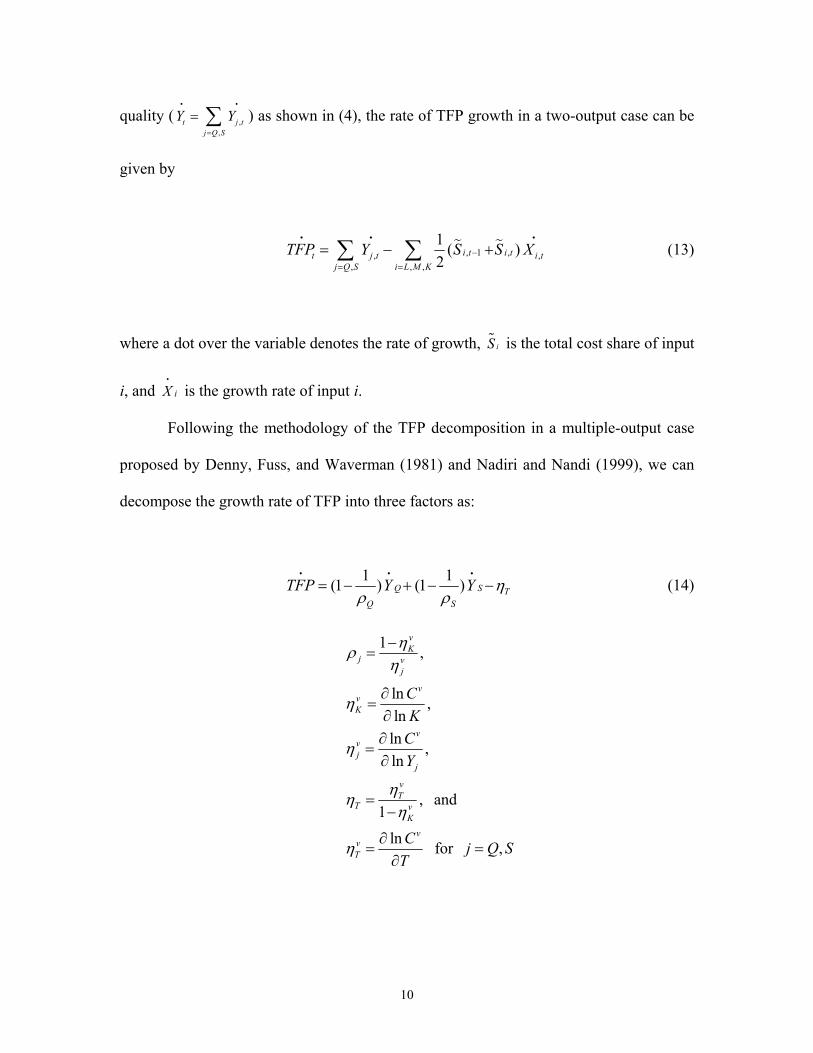
The growth rate of TFP is traditionally defined as the difference between the

growth rate of output and the growth rate of all inputs. Since the growth rate of the

quality-adjusted output (Y) is equal to the sum of growth rates of output quantity and

10

quality ( ,,

t j tj Q S

Y Y=

= ∑i i

) as shown in (4), the rate of TFP growth in a two-output case can be

given by

, 1 ,, ,, , ,

1 ( )2

i t i tt j t i tj Q S i L M K

TFP Y S S X−= =

= − +∑ ∑i i i

(13)

where a dot over the variable denotes the rate of growth, iS is the total cost share of input

i, and iXi

is the growth rate of input i.

Following the methodology of the TFP decomposition in a multiple-output case

proposed by Denny, Fuss, and Waverman (1981) and Nadiri and Nandi (1999), we can

decompose the growth rate of TFP into three factors as:

1 1(1 ) (1 )Q S TQ S

TFP Y Y ηρ ρ

= − + − −i i i

(14)

1 ,

ln ,ln

ln ,ln

, and1

ln for ,

vK

j vj

vvK

vvj

j

vT

T vK

vvT

CK

CY

C j Q ST

ηρη

η

η

ηηη

η

−=

∂=∂∂

=∂

=−

∂= =

∂

11

where vKη is the variable cost elasticity with respect to the capital stock, v

Qη and vSη are the

variable cost elasticities with respect to output quantity and quality, respectively, and vTη

is the variable cost elasticity with respect to the time variable. Scale economies are

measured as the inverse of cost elasticity with respect to output quantity. After correcting

for the effect of a quasi-fixed factor of the capital stock on the variable cost, Qρ measures

scale economies in the long-run. There are economies of scale if Qρ is greater than one.

In a similar vein, Sρ measures the degree of the cost efficiency for product innovation

which can be a source of productivity growth if Sρ is greater than one. Process-oriented

technical change can be measured with Tη− that represents a shift in the cost function.

On the right-hand side of equation (14), the first term is scale effect, the second

term is the effect of product innovation (quality effect), and the last term is the effect of

process innovation.6

3. Data

Data used in this study are obtained from the NBER-CES Manufacturing Industry

Database.7 Using the Annual Survey of Manufactures (ASM) and the Census of

Manufactures (CM), the NBER-CES database constructed the four-digit industry data on

gross output, employment, payroll, materials, capital stock, and various industry-specific

price indexes. Among the detailed industries, we use four computer industries as

6 Nadiri and Nandi (1998) decomposed scale effect into several exogenous components such as changes in exogenous demands, factor prices, etc. Unless either quantity or quality is assumed to be exogenous, we cannot decompose the scale and quality effects into other exogenous factors because of the property of the joint determination of quantity and quality. 7 See Bartelsman and Gray (1996) for the detailed description of the NBER-CES database.

12

Electronic computers (3571), Computer storage devices (3572), Computer terminals

(3575), and Computer peripheral equipment (3577) (SIC 1987 codes in parentheses)8.

However, the NBER-CES database covers only up to 1996, so we expanded the

database to 1999 with the latest publications of the ASM and CM. The industry

classification for the post-1996 data of the CM and ASM is based on the North American

Industry Classification System (NAICS). Using the bridge tables published by the Census

Bureau, all variables for the four industries are converted into those based on the SIC

1987.

Gross output in current prices is defined as the sum of shipments and changes in

inventories of finished goods. Using the ratio of the list price to the hedonic price as

shown in equation (2), we constructed the variable of output quality. We obtained the

hedonic price for computer products from the Bureau of Economic Analysis (BEA).9

The list price is obtained from the Current Industrial Reports (CIR) published by

the Census Bureau. The CIR includes the value of shipments as well as the quantity of

shipments in number of physical units. The list price was constructed by dividing the

nominal value of shipments by the physical units of shipments. Note that the BEA

hedonic prices are based on products rather than industries (BEA, 1998). For example,

the BEA estimated the hedonic price of printers, but did not provide the hedonic prices of

other computer peripheral equipment such as plotters and input-output devices that are

included in the computer peripheral equipment industry (SIC 3577). For consistency

8 We exclude Communication equipment (366) and Semiconductors and related devices (3674) because hedonic prices are not available for most products in Communication equipment and for Semiconductor-related devices. 9 See BEA (1998) for the details on sources and methods of the hedonic price indexes. The earlier hedonic price indexes constructed by the BEA are also found in Cole, Chen, Barquin-Stolleman, Dulberger, Helvacian, and Hodge (1986).

13

between the list and hedonic prices, we also constructed the list prices at the product

level. In contrast to the CM and ASM data, the CIR is not available before 1977.

Therefore, we restricted the sample period from 1977 to 1999.

Furthermore, we made some adjustments in variables in the NBER-CES database.

Since the payrolls in the NBER-CES database do not include supplemental labor costs of

social security contributions and fringe benefits, we include these supplemental costs into

the payrolls of workers. Since non-production worker hours are not available in the ASM

and CM data sets, production worker hours are used to construct the hourly wage rate of

all employees. The cost of materials measured in the CM and ASM data are adjusted in

two ways. The cost of purchased services is not included in the cost of materials in the

CM and ASM. The cost of purchased services obtained from the input-output tables, are

added into the cost of materials. Material inventories are also added into the cost of

materials: the work-in-process inventories are distributed into labor and materials using

the variable cost shares of inputs (Norsworthy and Jang, 1993).

We used the capital stock from the NBER-CES database that converted the 3-digit

level capital stock constructed by the Board of Governors of the Federal Reserve System

(FRB) into the 4-digit level by assuming that the asset types are the same for all 4-digit

industries within a common 3-digit industry.10 The before-tax user cost of capital is

defined as:

(1 )( )1

K K K KK

q uz rWu

ζ δ− − +=

−

14

where qK is the investment price deflator, ζK is the rate of investment tax credit, u is the

corporate income tax rate, δK is the depreciation rate of capital, zK is the present value of

capital consumption allowances, and r is the real rate of return.

[Table 1]

Table 1 presents the average annual growth rate of each variable for the period

1978-1999. The hedonic price fell at an annual rate of 16.87 percent on average for the

four computer industries. In particular, the hedonic price in the electronic computers

industry decreased more rapidly than those in the other three industries. However, the

growth rate of the hedonic price is not necessarily the same as the growth rate of quality

because the hedonic price also falls as the list price decreases. The growth rate of quality

is defined as the growth rate of the list price minus the growth rate of the hedonic price.

A lower hedonic price as well as a higher list price can result in a better quality. In

addition to declines in the hedonic prices, the list prices have also fallen for all

industries.11

After correcting for changes in the list prices, the annual growth rate of the quality

improvement is about 12 percent on average for all industries from 1978 to 1999. This

suggests that the improvement in true quality is smaller than changes in the hedonic

price. Quality improvements are significantly different across industries. In particular, the

10 See Mohr and Gilbert (1996) for the description of the FRB 3-digit capital data. 11 For example, Berndt, Dulberger, and Rappaport (2001) reported the list prices of desktop and mobile computers during the last quarter-century, and found that the list price of desktop computers rose annually by 6.8 percent between 1976 and 1989, and then fell again annually by 13.0 percent between 1989 and 1999.

15

quality improvement in electronic computers has been faster than those in the other three

computer products.

In a similar way, the growth rate of output quantity is defined as the growth rate

of the nominal output minus the growth rate of the list price. The average annual growth

rate of quantity is about 15 percent for all industries. Except for the computer terminals

industry, the annual growth rates of output quantity for the other three industries are

between 13.28 and 15.71 percent. This implies that the computer industries have a

smaller variation in the growth rate of quantity than in that of quality.

The growth rate of the quality-adjusted output, that is the sum of the growth rates

of quantity and quality, is about 27 percent. This implies that quality improvement

contributes almost a half of the growth of the quality-adjusted output.

In contrast to a rapid growth of both output quantity and quality, the growth rates

of labor and capital inputs are relatively low. In particular, the growth rate of labor input

has been almost constant. Warnke (1996) found that the computer industry enjoyed a

faster growth in employment between 1960 and 1984, but began to shed jobs rapidly

from 1984 to 1995. She argues that employment declines, especially associated with

cutting low skilled and production workers, are attributable to changes in market

structure, a faster factory automation, and international competition.12

4. Empirical Results

We estimate a system of equations consisting of the variable cost function, the

variable cost share equations of labor and capital, and two optimality conditions for

16

output quantity and quality using the non-linear three-stage least squares (3SLS). We use

a set of instrumental variables: lagged variables and a few macroeconomic variables such

as oil price, military expenditures, and the number of population.

[Table 2]

The optimal choice of output quantity and quality depends on two different

demand conditions as well as cost structures that are jointly estimated in this study. The

parameter estimates of the model are shown in Table 2 and the majority of the parameter

estimates are statistically significant. We introduced the industry dummy variables for

intercepts in all equations, and also allow the industry dummy variables for time

coefficient to capture different process innovations among the four industries.

Demand Elasticity and Markup

In Table 2, the coefficient estimate of αQ is about –0.33, which implies that the

quantity demand elasticity with respect to the list price, holding output quality constant,

is about -3.05. The estimate of the inverse demand elasticity with respect to quantity is

similar to the findings of Stavins (1997) which estimated the demand elasticities for

personal computers (PCs) using micro-level data between 1976 and 1988.13 After

controlling for characteristics of differentiated products, she found relatively elastic price

12 The productivity growth in the computer industry could be affected by this change in the production structure. 13 Without correcting for changes in product quality, an earlier study of Chow (1967) found that the demand elasticity for mainframe computers is close to -1. Using the data from the banking and insurance firms in the late 1980s, however, a recent study by Hendel (1999) found more elastic demand for PCs than

17

demand elasticities ranging between -2.9 and -7.2. Our estimate of the quantity demand

elasticity is close to the lower bound of Stavins’ estimates. Since we expect that the

demand for mainframe computers is less elastic than the demand for PCs, the average

demand elasticity, including all types of electronic computers, may be lower than that of

PCs. However, there are few comparable studies on the demand elasticities for the other

computer industries such as storage devices, terminals, and printers. This estimate of the

demand elasticity implies that the markup for output quantity is about 0.49.

The coefficient estimate of αS in Table 2 implies that the demand elasticity with

respect to output quality is 1.91. The finding suggests that the quality demand is less

elastic than the quantity demand, and subsequently the markup associated with quality is

greater than that associated with quantity. Hence, this suggests that the computer product

market is more competitive in quantity than in quality.

Using the data for 19 OECD countries, Oliveira-Martins, Scarpetta, and Pilat

(1996) estimated markups for 36 manufacturing industries at the 3-digit level. In their

results, higher markups were estimated for tobacco products, drugs and medicines, and

office and computing machinery, while lower markups were estimated for footwear,

wearing apparel, and motor vehicles. Their markup estimate for office and computing

machinery industry from 1970 to 1992 is about 0.6, which is very high. Their estimate

lies between our markup estimates of the output quantity and quality. This implies that

without distinguishing the demand for output quantity and quality, the average markup

can overestimate the markup associated with quantity and can underestimate that

associated with quality. Furthermore, a high markup in the computer industry is in part

those of Stavins (1997). See Davis (2000) for an overview of modeling the demand for differentiated products.

18

due to a high markup associated with quality. In other words, a high markup in this

industry can be attributed to technological characteristics rather than to the market

power.14

Cost Elasticity and Scale

Table 3 presents the short-run and long-run cost elasticities with respect to output

quantity and quality, input prices, a quasi-fixed factor of the capital stock, and time

variable. The short-run implies that production is conducted when the level of the capital

stock is fixed.

[Table 3]

The short-run variable cost elasticity of output quantity is 0.86 implying that a 1

percent increase in the production of output quantity incurs an increase of about 0.86

percent in the variable cost. One of the interesting results is that the cost elasticity of

output quality is smaller than that of output quantity. This suggests that the production of

14 A time-series pattern of markup is an interesting issue because it gives a hint for changes in the market structure of the computer industry. For example, Stavins (1997) showed that the demand elasticity for PCs rose between 1977 and 1988 because of the entrance of several IBM-compatible PCs. This implies that the PC industry became more competitive in this period. However, the number of firms in the PC industry increased between 1978 and 1990, but decreased between 1990 and 1999, which suggests that there could be a possible structural break in the nature of competition in the pre- and post-1990 periods. However, it is difficult to conclude that the computer market became less competitive in the 1990s based on the observed trend in the number of firms. Filson (2001) showed that the number of firms in the electronic computer marker increased from the 1970s to the 1980s, but decreased from the 1990s while those in the printer market increased from the 1970s to the 1990s. Stavins (1995) also examined the entry and exit of firms in the PC market. To explain changes in the market structure of the computer industry, Bresnahan and Greenstein (1999) suggest technological competition between computer platforms, not firms, and find that competition in the computer market changed little over time with the aspect of platform competition. Since we formulate the model with time-invariant markups for quantity and quality, this issue is beyond the scope of this paper.

19

quality entails less cost than the production of quantity. Positive signs of cost elasticities

with respect to labor and materials prices imply that higher input prices incur larger costs

of production. The variable cost elasticity of the time variable suggests that the variable

cost has declined about 7.7 percent annually, given production of the same amount of

output quantity and quality.

In the long-run, cost can be minimized with the adjustment of capital. Hence, we

may expect that the cost elasticities are smaller in the long-run than in the short-run. For

example, the cost elasticity of output quantity of 0.79 in the long-run is smaller than 0.86

in the short-run.

Scale economies arise when production expansion causes a less than proportional

increase in inputs and therefore in costs. Thus, scale economies are considered as a

source of productivity growth. However, scale economies are different from technical

change because lower unit costs of production are associated with the expansion of

production via larger sizes of plants. In contrast to a case of the homogenous product,

production expansion in the computer industry does not properly represent increases in

output quantity because production can increase with more quantity as well as with more

quality. If we measure the quantity of output with a conventional method, i.e., deflating

the nominal value of output by the hedonic price, the production expansion based with

this output can take place in both producing a better product and producing more units of

the same product.15

Note that scale economies can be measured as the inverse of cost elasticity with

respect to output quantity after controlling for technical changes. Unless we distinguish

20

the production expansion through improvements in product quality from increases in

physical units of output, a conventional scale estimate measures the average of the

marginal cost associated with better quality as well as the marginal cost associated with

more quantity. Therefore, in this paper, we assume that scale economies can arise only

through the expansion of physical units of product, given quality. The output expansion

effect through quality improvement on changes in costs can be regarded as a different

source of productivity growth.

Scale estimates in both the long-run and short-run for all four industries are

greater than one, which suggests the presence of increasing returns to scale. The scale in

the long-run is on average 1.16. In particular, the scale is slightly smaller in the electronic

computers industry than in the other three industries.

Decomposition of TFP Growth

Using the methodology described in equation (14), Table 4 presents the

decomposed contribution to TFP growth: the effects of process and product innovations

and scale effect. First row in Table 4 shows the TFP growth rates for the four computer

industries. The TFP growth rate in the electronic computers industry (SIC 3571) is

approximately 18 percent and is the highest among the four industries. The TFP growth

rate in the terminals industry is only one-third of the rate in the electronic computers

industry. An average TFP growth rate for the four industries is about 15 percent, but the

TFP growth rates are very heterogeneous among the industries.

15 Klette and Griliches (1996) emphasize inconsistency in scale estimators due to the use of inaccurate prices of output in a differentiated product market. In their study, the inconsistency can arise when firms produce differentiated products and their outputs are deflated by a common industry output price.

21

[Table 4]

The contribution of process innovation is on average about 7 percent, which

accounts for almost half of the TFP growth. However, product innovation associated with

better quality appears to be an important contributor as well, explaining about 30 percent

of the TFP growth in the computer industries, while scale effect explains only about 20

percent of the TFP growth. The results imply that the sum of process and product

innovations in total explains more than three-fourths of the TFP growth.16 The results

also suggest that the productivity growth in the computer industries mainly depends upon

the technical changes and, subsequently, is not likely to be vulnerable to changes in the

demand for computer products.

Except for the storage devices industry (SIC 3572), the technical change due to

process innovation explains about half of the TFP growth and the product-oriented

technical change explains about one-third of the TFP growth. In the storage devices

industry, scale effect accounts for almost half of the TFP growth and the product-oriented

technical change accounts for one-third of the TFP growth, while the contribution of the

process innovation is relatively small. The storage devices industry is an industry

producing components of computers while the other three industries mainly produce final

products of computers and peripherals. Thus, we can expect that the production structure

16 In contrast to our estimation results, the study by Nadiri and Prucha (1990) on the U.S. electrical machinery industry (SIC 36) from 1960 to 1980 found that the scale effect including temporary equilibrium and adjustment cost effects explains about two-thirds of the TFP growth, and technical change explains the remaining one-third. Since the electrical machinery industry includes communications equipment and semiconductors, we also expect a rapid quality improvement in this industry. Hence, their scale estimate may be overestimated because they didn’t distinguish the output expansion through the quality improvement from the total output expansion.

22

of the storage devices industry may be close to that of the semiconductor industry

producing microprocessors and memory chips. Since the storage devices industry

develops similar types of products such as hard disks and floppy diskettes and produces

on a large scale with a simpler production process than the other three computer

industries, we may expect that effects of product innovation and economies of scale are

more important than the effect of process innovation.17

5. Implications for Productivity Growth in the Aggregate

Economy

Table 5 shows the TFP growth rate in the U.S. nonfarm business sector for

various periods published by the Bureau of Labor Statistics (BLS). From 1995 through

1999, there was a remarkable resurgence in the productivity growth from the first half of

the 1990s. Determining the source of the productivity resurgence in the aggregate

economy, some recent studies (Jorgenson and Stiroh, 2000; Oliner and Sichel, 2000;

Whelan, 2002) focus on the role of the IT-producing industry such as computers,

communications equipment, and semiconductors.

[Table 5]

17 Although we decomposed the TFP growth in the computer industry into the three factors, it is worthwhile to pursue the following question. Which factor determines the relative importance of process and product innovations? Differences in R&D expenditures in product and process innovations in the computer industry can be a possible answer. Another possible answer can be the difference in the effect of learning-by-doing. For example, Irwin and Klenow (1994) found a strong effect of learning-by-doing on the cost reduction in the semiconductor industry.

23

Table 5 also shows that the TFP growth rate in the computer industry accelerated

from the early 1990s to the late 1990s. We also compare our TFP growth rate in the

computer industry with that of Oliner and Sichel (2000) measured by the dual approach.

The TFP growth rate in this study for the period of 1978-1995 is similar to that of their

study. The TFP growth rates are different between this study and their study during the

second half of the 1990s. One of the main reasons for the difference is that Oliner and

Sichel (2000) assume the same cost structure between the IT-producing industry and

other industries.

Using the TFP growth rate in the computer industry, we measure the contribution

from the computer industry to the TFP growth in the aggregate economy, in particular,

the nonfarm business sector. The industry productivity measure, however, is not directly

comparable to the aggregate one because the productivity measure for the aggregate

economy uses value-added while the productivity measure for the industry uses gross

output. To measure the contribution of the computer industry to the aggregate TFP

productivity growth, we use the methodology developed by Domar (1967). The

contribution of the computer industry to the aggregate TFP growth can be obtained from

a weighted sum of the TFP growth rates of the computer industries with the Domar

weights equal to the ratios of industry gross output to aggregate value-added:

4

1t it it

iTFP w TFP

=

= ∑i i

(15)

where wit is the Domar weight for industry i at time period t.

24

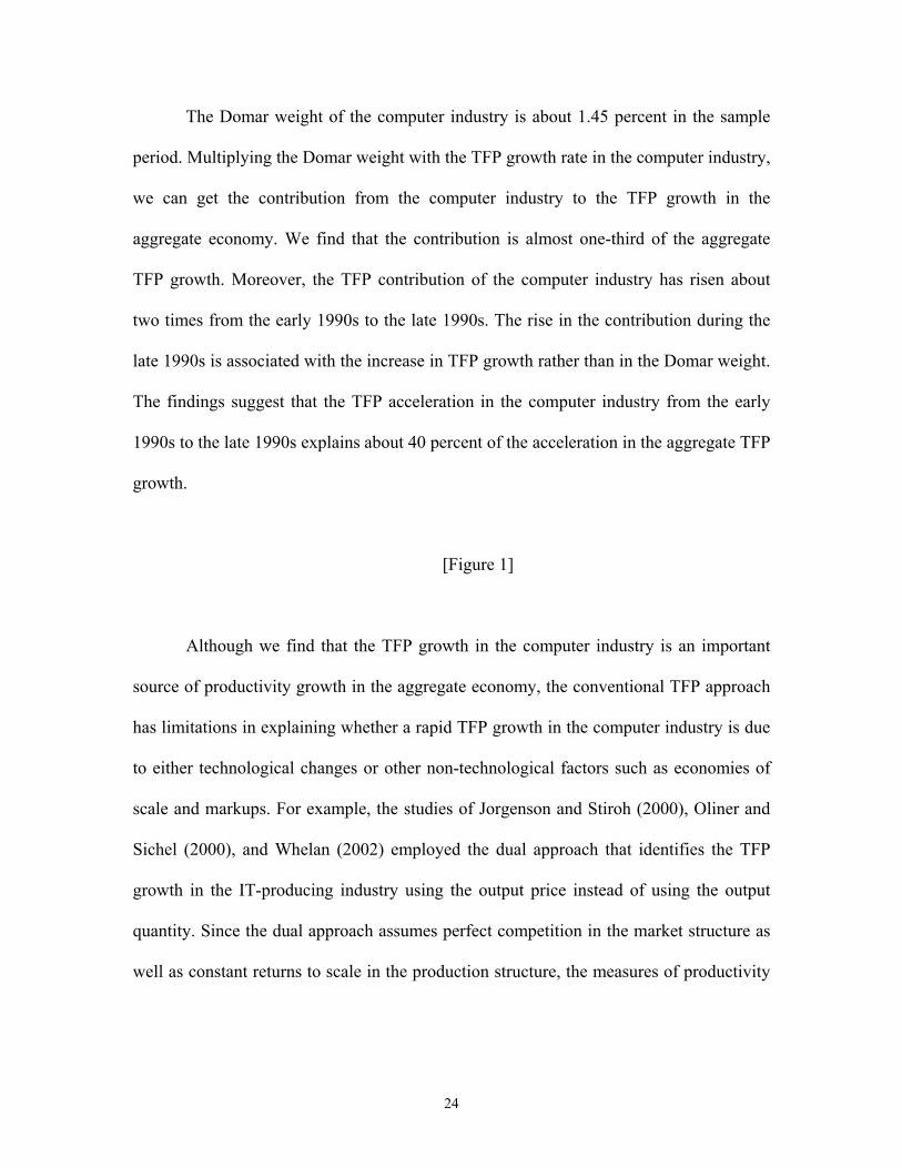
The Domar weight of the computer industry is about 1.45 percent in the sample

period. Multiplying the Domar weight with the TFP growth rate in the computer industry,

we can get the contribution from the computer industry to the TFP growth in the

aggregate economy. We find that the contribution is almost one-third of the aggregate

TFP growth. Moreover, the TFP contribution of the computer industry has risen about

two times from the early 1990s to the late 1990s. The rise in the contribution during the

late 1990s is associated with the increase in TFP growth rather than in the Domar weight.

The findings suggest that the TFP acceleration in the computer industry from the early

1990s to the late 1990s explains about 40 percent of the acceleration in the aggregate TFP

growth.

[Figure 1]

Although we find that the TFP growth in the computer industry is an important

source of productivity growth in the aggregate economy, the conventional TFP approach

has limitations in explaining whether a rapid TFP growth in the computer industry is due

to either technological changes or other non-technological factors such as economies of

scale and markups. For example, the studies of Jorgenson and Stiroh (2000), Oliner and

Sichel (2000), and Whelan (2002) employed the dual approach that identifies the TFP

growth in the IT-producing industry using the output price instead of using the output

quantity. Since the dual approach assumes perfect competition in the market structure as

well as constant returns to scale in the production structure, the measures of productivity

25

growth in these studies could be overestimated if the output price is above the marginal

cost, implying a positive markup (Hobijn, 2001) or scale economies prevail.

Table 5 reports the decomposition results of the computer industry’s contribution

to the aggregate TFP growth. First, the scale effect explains almost 20 percent of the

contribution, which suggests that one-fifth of the contribution is associated with non-

technological factors.

Table 5 also shows interesting trends in decompositions of the TFP contribution.

In particular, the contribution from product innovation rose rapidly in the later part of the

sample period while the contribution from process innovation and economies of scale

changed little. Filson (2001) also finds an increasing trend in product innovation in the

computer industry, but a decreasing trend in the automobile industry. The time-series

pattern of product and process innovations in the computer industry challenges the

prediction of the industry life-cycle theory that new industries experience product

innovation early and process innovation later (Gort and Klepper, 1982; Klepper, 1996).

Although the contribution of process innovation to the TFP growth in the

aggregate economy is greater than that of product innovation, an increase in the product-

oriented technical change in the late 1990s explains about 60 percent of the acceleration

in the computer industry’s TFP contribution. The contribution from the non-technological

factor of scale economies also changed little from the early to the late 1990. Therefore,

the findings suggest that the productivity acceleration in the aggregate economy

associated with the computer industry during the late 1990s is largely attributable to

acceleration in the technical change due to product innovation in the computer industry.

26

6. Conclusion

In this paper, we provide an empirical framework for exploring the different

sources of the productivity growth in the U.S. computer industries. We decomposed the

conventionally measured TFP growth into three components: process and product

innovations and economies of scale. The empirical results of this study show that a

technological change associated with both process and product innovations has been a

major source of the TFP growth in the computer industry.

For the sample period of 1978-1999, process innovation explains almost half of

the TFP growth in the computer industry, while product innovation associated with better

quality accounts for about 30 percent of the TFP growth. Furthermore, the contribution

from product innovation to the TFP growth has increased during the sample period, while

the contribution from process innovation has changed little and the contribution from

economies of scale has declined. In particular, the TFP acceleration in the computer

industry in the late 1990s is mainly derived from a rapid increase in product innovation.

The findings on the time-series patterns of product and process innovations in this

paper cast doubt on the prediction of the industry life-cycle theory, which suggests that

new industries experience product innovation early and process innovation later. We have

not explored the determinants of an increasing trend in product innovation in the

computer industry. We intend to address this issue in future work.

27

References

Bartelsman, Eric J. and Wayne Gray, “The NBER Productivity Database,” NBER

Technical Working Paper No. 205, October 1996.

Berndt, Ernst R., Ellen R. Dulberger, and Neal J. Rappaport, “Price and Quality of

Desktop and Mobile Computers: A Quarter Century Historical Overview,” American

Economic Review, 91(2), May 2001, 268-73.

Bresnahan, Timothy F. and Shane Greenstein, “Technological Competition and the

Structure of the Computer Industry,” Journal of Industrial Economics, 47(1), March

1999, 1-40.

Bureau of Economic Analysis, “Computer Prices in the National Accounts: An Update

from the Comprehensive Revision,” National Income and Wealth Division Working

Paper, Bureau of Economic Analysis, August 1998.

Bureau of Labor Statistics, Multifactor Productivity Trends, 1999, Bureau of Labor

Statistics, May 2001.

Chow, Gregory C., “Technological Change and the Demand for Computers,” American

Economic Review, 57(5), December 1967, 1117-30.

Cole, Rosanne, Y. C. Chen, Joan A. Barquin-Stolleman, Ellen R. Dulberger, Nurhan

Helvacian, and James H. Hodge, “Quality-Adjusted Price Indexes for Computer

Processors and Selected Peripheral Equipment,” Survey of Current Business, 66(1),

January 1986, 41-50.

Davis, Peter, “Empirical Models of Demand for Differentiated Products,” European

Economic Review, 44(4-6), May 2000, 993-1005.

Denny, Michael, Melvyn Fuss, and Leonard Waverman “The Measurement and

Interpretation of Total Factor Productivity in Regulated Industries, with an Application to

Canadian Telecommunications,” in Thomas G. Cowing and Rodney E. Stevenson, (eds.),

28

Productivity Measurement in Regulated Industries, New York: Academic Press, 1981,

179-218.

Domar, Evsey, “On the Measurement of Technological Change,” Economic Journal,

71(284), December 1961, 709-29.

Dorfman, Robert and Peter O. Steiner, “Optimal Advertising and Optimal Quality,”

American Economic Review, 44(5), December 1954, 826-36.

Filson, Darren, “The Nature and Effects of Technological Change over the Industry Life

Cycle,” Review of Economic Dynamics, 4(2), 2001, 460-94.

Gort, Michael and Steven Klepper, “Time Paths in the Diffusion of Product Innovations,”

Economic Journal, 92(367), September 1982, 630-53.

Hendel, Igal, “Estimating Multiple-Discrete Choice Models: An Application to

Computerization Returns,” Review of Economic Studies, 66(2), April 1999, 423-46.

Hobijn, Bart, “Is Equipment Price Deflation a Statistical Artifact?” Federal Reserve Bank

of New York Staff Reports No. 139, November 2001.

Hulten, Charles R. “Total Factor Productivity: A Short Bibliography,” in Charles R.

Hulten, Edwin R. Dean, and Michael J. Harper (eds.), New Developments in Productivity

Analysis, Chicago: University of Chicago Press, 2001, 1-47.

Irwin, Douglas A. and Peter J. Klenow, “Learning-by-Doing Spillovers in the

Semiconductor Industry,” Journal of Political Economy, 102(6), December 1994, 1200-

27.

Jorgenson, Dale W. and Kevin J. Stiroh, “Rising the Speed Limit: U.S. Economic Growth

in the Information Age,” Brookings Papers on Economic Activity, (1), 2000, 125-233.

Klepper, Steven, “Entry, Exit, and Innovation over the Product Life Cycle,” American

Economic Review, 86(3), June 1996, 562-83.

29

Klette, Tor Jakob and Zvi Griliches, “The Inconsistency of Common Scale Estimators

When Output Prices Are Unobserved and Endogenous,” Journal of Applied

Econometrics, 11(4), July-August 1996, 343-61.

Kremer, Michael, “The O-ring Theory of Economic Development,” Quarterly Journal of

Economics, 108(3), August 1993, 551-75.

Mohr, Michael F. and Charles E. Gilbert, “Capital Stock Estimates for Manufacturing

Industries: Methods and Data,” Board of Governors of the Federal Reserve System,

March 1996.

Nadiri, M. Ishaq and Banani Nandi, “Technical Change, Markup, Divestiture, and

Productivity Growth in the U.S. Telecommunications Industry,” Review of Economics

and Statistics, 81(3), August 1999, 488-98.

Nadiri, M. Ishaq and Ingmar R. Prucha, “Comparison and Analysis of Productivity

Growth and R&D Investment in the Electrical Machinery Industries of the United States

and Japan,” in Charles. R. Hulten, (ed.), Productivity Growth in Japan and the U.S.,

Chicago: University of Chicago Press, 1990, 109-33.

Nadiri, M. Ishaq and Ingmar R. Prucha, “Dynamic Factor Demand Models and

Productivity Analysis,” in Charles. R. Hulten, Edwin R. Dean, and Michael J. Harper

(eds.), New Developments in Productivity Analysis, Chicago: University of Chicago

Press, 2001, 103-64.

Norsworthy, John R. and Show-Ling Jang, “Cost Function Estimation of Quality Change

in Semiconductors,” in Murray F. Foss, Marilyn E. Mansor, and Allen H. Young (eds.),

Price Measurements and Their Uses, Chicago: Chicago University Press, 1993, 125-55.

Ohta, Makoto, “Production Technologies of the U.S. Boiler and Turbo Generator

Industries and Hedonic Price Indexes for Their Products: A Cost-Function Approach,”

Journal of Political Economy, 83(1), February 1975, 1-26.

30

Oliner, Stephen D. and Daniel E. Sichel, “The Resurgence of Growth in the Late 1990s:

Is Information Technology the Story?” Journal of Economic Perspectives, 14(4), Fall

2000, 3-22.

Oliveira-Martins,-Joaquim, Stefano Scarpetta, and Dirk Pilat, “Mark-Up Pricing, Market

Structure and the Business Cycle,” OECD Economic Studies, (27), 1996, 71-105.

Raff, Daniel M. G. and Manuel Trajtenberg, “Quality-Adjusted Prices for the American

Automobile Industry: 1906-1940,” in Timothy F. Bresnahan and Robert J. Gordon (eds.),

The Economics of New Good, Chicago: University of Chicago Press, 1997, 71-101.

Rosen, Sherwin, “Hedonic Prices and Implicit Markets: Product Differentiation in Pure

Competition,” Journal of Political Economy, 82(1), January-February 1974, 34-55.

Stavins, Joanna, “Model Entry and Exit in a Differentiated-Product Industry: The

Personal Computer Market,” Review of Economics and Statistics, 77(4), November 1995,

571-84.

Stavins, Joanna, “Estimating Demand Elasticities in a Differentiated Product Industry:

The Personal computer Market,” Journal of Economics and Business, 49(4), July-August

1997, 347-67.

Thompson, Peter and Doug Waldo, “Process versus Product Innovation: Do

Consumption Data Contain Any Information?” Southern Economic Journal, 67(1), July

2000, 155-70.

Warnke, Jacqueline, “Computer Manufacturing: Change and Competition,” Monthly

Labor Review, 119(8), August 1996, 18-29.

Whelan, Karl, “Computers, Obsolescence, and Productivity,” Review of Economics and

Statistics, 84(3), August 2002, 445-61.

Yorukoglu, Mehmet, “Product vs. Process Innovations and Economic Fluctuations,”

Carnegie-Rochester Conference Series on Public Policy, 52(1), June 2000, 137-63.

31

Table 1. Summary Statistics: 1978-1999

(Average annual growth rates in percentage)

Electronic computers

Computer storage devices

Computer terminals

Computer peripheral equipment

Average

(3571) (3572) (3575) (3577) Outputs Nominal output 10.20 11.08 0.84 9.17 9.91List price -5.51 -2.20 -4.04 -5.37 -4.93Hedonic price -20.47 -8.59 -8.37 -12.85 -16.87Quantity of output 15.71 13.28 4.88 14.54 14.83Quality of output 14.96 6.38 4.34 7.48 11.95 Inputs Quantity of labor input -0.38 1.93 -4.76 2.32 0.39Quantity of materials 16.14 16.06 6.46 14.71 15.65Quantity of capital stock 6.65 9.80 4.58 8.80 7.51Price of labor input 5.45 4.83 4.30 5.65 5.38Price of materials -5.00 -4.81 -4.59 -4.83 -4.92Rental price of capital stock 2.16 2.29 2.28 2.26 2.21

Note: Average growth rates of the four industries are weighted by the industry share of nominal output between two adjacent years. The growth rate of output quantity is equal to the growth rate of nominal output minus the growth rate of list price. The growth rate of output quality is equal to the growth rate of list price minus the growth rate of hedonic price.

32

Table 2. Estimation Results

Parameter Estimate Standard Error Β0 6.4820 0.4521 Β02 (dummy) -1.9822 0.2256 Β03 (dummy) -1.8254 0.3105 Β04 (dummy) -0.5309 0.1985 BL 0.8703 0.1124 ΒL2 (dummy) 0.0336 0.0152 ΒL3 (dummy) 0.0074 0.0297 ΒL4 (dummy) 0.0230 0.0139 ΒK 0.0982 0.0771 ΒK2 (dummy) -0.0464 0.0151 ΒK3 (dummy) -0.1058 0.0303 ΒK4 (dummy) -0.0222 0.0141 ΒQ 0.5496 0.0882 ΒQ2 (dummy) -0.0544 0.0248 ΒQ3 (dummy) -0.0164 0.0404 ΒQ4 (dummy) -0.0727 0.0206 ΒS 0.4737 0.0696 ΒS2 (dummy) -0.0498 0.0190 ΒS3 (dummy) -0.0384 0.0308 ΒS4 (dummy) -0.0682 0.0162 ΒT -0.1642 0.0270 ΒT2 (dummy) 0.0910 0.0069 ΒT3 (dummy) 0.0710 0.0105 ΒT4 (dummy) 0.0473 0.0061 ΒLL 0.0939 0.0312 ΒKK -0.0815 0.0135 ΒQQ 0.0012 0.0102 ΒSS 0.0089 0.0059 ΒTT 0.0018 0.0008 ΒLK 0.0000 0.0134 ΒLQ -0.0235 0.0080 ΒLE -0.0208 0.0061 ΒLT -0.0128 0.0026 ΒKQ 0.0419 0.0073 ΒKS 0.0142 0.0048 ΒKT -0.0001 0.0014 ΒQS 0.0087 0.0072 ΒQT 0.0007 0.0019 ΒST 0.0010 0.0014 AQ -0.3275 0.0336 AS 0.5236 0.0270 Equation Standard Error R2 Variable cost equation 0.0847 0.9957 Labor share equation 0.0205 0.9069 Capital share equation 0.0213 0.5192 Output quantity equation 0.0686 0.6236 Output quality equation 0.0688 0.6213

33

Table 3. Short-run and Long-run Cost Elasticities and Scales

Electronic

computers Computer

storage devices

Computer terminals

Computer peripheral equipment

Average

(3571) (3572) (3575) (3577) Short-run Quantity of output 0.909 0.804 0.774 0.786 0.864Quality of output 0.708 0.626 0.603 0.612 0.673Time -0.101 -0.011 -0.032 -0.055 -0.077Price of labor input 0.227 0.300 0.308 0.281 0.251Price of materials 0.773 0.700 0.692 0.719 0.749Capital stock -0.093 -0.120 -0.109 -0.073 -0.092Scale 1.100 1.245 1.291 1.272 1.163 Long-run Quantity of output 0.833 0.718 0.698 0.733 0.791Quality of output 0.648 0.559 0.544 0.571 0.616Time -0.092 -0.010 -0.029 -0.051 -0.070Price of labor input 0.207 0.268 0.278 0.262 0.229Price of materials 0.709 0.624 0.624 0.671 0.687Scale 1.202 1.394 1.432 1.365 1.271

Note: Average elasticities and scales of the four industries are weighted by the industry share of nominal output between two adjacent years.

34

Table 4. Decompositions of TFP Growth in Computer Industries: 1978-1999

(in percentage)

Electronic computers

Computer storage devices

Computer terminals

Computer peripheral equipment

Average

(3571) (3572) (3575) (3577) TFP growth rate 18.46 8.00 6.00 10.91 15.06 Scale effect 2.76 3.83 1.38 3.87 3.12 Effect of product innovation 5.08 2.76 2.01 3.18 4.30 Effect of process innovation 9.24 0.97 2.86 5.10 7.03 Residuals 1.38 0.44 -0.26 -1.24 0.60 Industry output share 0.62 0.13 0.03 0.22 Note: Average rates of the four industries are weighted by the industry share of nominal output between two adjacent years.

35

Table 5. Contribution of the Computer Industry to TFP Growth

in the Nonfarm Business Sector

1978-1990 1991-1995 1996-1999 1978-1999

TFP growth rate in the nonfarm business sector: BLS (2001) 0.30 0.60 1.10 0.51 TFP growth rate in the computer industry: Oliner and Sichel (2000) 11.2a 11.3 16.6 12.2b This study 13.98 12.37 22.05 15.06 Domar weight of the computer industry: Oliner and Sichel (2000) 1.1a 1.4 1.6 1.2b This study 1.42 1.35 1.64 1.45 Contribution from the computer industry to TFP growth in the nonfarm business sector: Oliner and Sichel (2000) 0.12a 0.16 0.26 0.15b This study Total contribution 0.19 0.17 0.37 0.22 Scale effect 0.05 0.03 0.02 0.04 Effect of product innovation 0.04 0.05 0.17 0.07 Effect of process innovation 0.10 0.09 0.11 0.10 Residuals 0.00 -0.01 0.07 0.01 Notes: Domar weight is defined as the ratio of gross output in the computer industry to value-added in the nonfarm business sector. a includes the period of 1974-1990. b includes the period of 1974-1999.

36

Figu

re 1

. Con

trib

utio

n fr

om th

e C

ompu

ter I

ndus

try

to T

FP G

orw

th in

the

Non

farm

Bus

ines

s Se

ctor

-0.2

0

-0.1

0

0.00

0.10

0.20

0.30

0.40

0.50

0.60

1978

1979

1980

1981

1982

1983

1984

1985

1986

1987

1988

1989

1990

1991

1992

1993

1994

1995

1996

1997

1998

1999

Tota

l C

ontri

butio

nPr

oduc

t inn

ovat

ion

Proc

ess

inno

vatio

n

Scal

e ef

fect