NBER WORKING PAPER SERIES

HISTORY REMEMBERED:OPTIMAL SOVEREIGN DEFAULT ON DOMESTIC AND EXTERNAL DEBT

Pablo D'ErasmoEnrique G. Mendoza

Working Paper 25073http://www.nber.org/papers/w25073

NATIONAL BUREAU OF ECONOMIC RESEARCH1050 Massachusetts Avenue

Cambridge, MA 02138September 2018

We thank Alessandro Dovis, Gita Gopinath, Jonathan Heathcote, Alberto Martin, Vincenzo Quadrini and Martin Uribe for helpful comments and suggestions, and also gratefully acknowledge comments by conference and seminar participants at the European University Institute, UC Santa Barbara, Centre de Recerca en Economia Internacional, International Monetary Fund, the Stanford Institute for Theoretical Economics, Riskbank, the Atlanta and Richmond Federal Reserve Banks, the 2013 SED Meetings and the NBER Summer Institute meeting of the Macroeconomics Within and Across Borders group, the 2014 North American Summer Meeting of the Econometric Society, and ITAM-PIER conference. We also acknowledge the support of the National Science Foundation through grant SES-1325122. An earlier version of this paper circulated under the title “Optimal Domestic Sovereign Default.” The views expressed in this paper do not necessarily reflect those of the Federal Reserve Bank of Philadelphia, the Federal Reserve System, or the National Bureau of Economic Research.

NBER working papers are circulated for discussion and comment purposes. They have not been peer-reviewed or been subject to the review by the NBER Board of Directors that accompanies official NBER publications.

© 2018 by Pablo D'Erasmo and Enrique G. Mendoza. All rights reserved. Short sections of text, not to exceed two paragraphs, may be quoted without explicit permission provided that full credit, including © notice, is given to the source.

History Remembered: Optimal Sovereign Default on Domestic and External DebtPablo D'Erasmo and Enrique G. MendozaNBER Working Paper No. 25073September 2018JEL No. E44,E6,F34,H63

ABSTRACT

Infrequent but turbulent overt sovereign defaults on domestic creditors are a “forgotten history” in Macroeconomics. We propose a heterogeneous-agents model in which the government chooses optimal debt and default on domestic and foreign creditors by balancing distributional incentives v. the social value of debt for self-insurance, liquidity, and risk-sharing. A rich feedback mechanism links debt issuance, the distribution of debt holdings, the default decision, and risk premia. Calibrated to Eurozone data, the model is consistent with key long-run and debt-crisis statistics. Defaults are rare (1.2 percent frequency), and preceded by surging debt and spreads. Debt sells at the risk-free price most of the time, but the government's lack of commitment reduces sustainable debt sharply.

Pablo D'ErasmoFederal Reserve Bank of PhiladelphiaResearch DepartmentTen Independence Mall, Philadelphia PA 19106pabloderasmo@gmail.com

Enrique G. MendozaDepartment of EconomicsUniversity of Pennsylvania3718 Locust WalkPhiladelphia, PA 19104and NBERegme@sas.upenn.edu

A data appendix is available at http://www.nber.org/data-appendix/w25073

In loving memory of Dave Backus

1 Introduction

The central finding of the seminal cross-country analysis of the history of public debt by

Reinhart and Rogoff [48] is that governments defaulted outright on their domestic debt

68 times over the past 250 years. The United States is no exception. Hall and Sargent

[34] document in detail the domestic default that followed the American Revolutionary War.

These are de jure defaults in which governments reneged on the contractual terms of domestic

debt via forcible conversions, lower coupon rates, reductions of principal and suspension of

payments, separate from de facto defaults due to inflation or currency devaluation. Overt

domestic defaults are rare, with an unconditional frequency of about 1.1 percent in the

Reinhart-Rogoff dataset (68 events for 64 countries, with data for most covering the 1914-

2007 period and for some since 1750), but they are turbulent episodes in terms of financial

instability and macroeconomic performance. Also, all of the domestic defaults triggered

external defaults, in some cases even at low external debt ratios.1 Despite these striking

facts, Reinhart and Rogoff found that domestic defaults represent a “forgotten history” in

the Macroeconomics literature.

Recent events raising the prospect of domestic defaults in advanced economies make

this history much harder to forget. The European debt crisis, historically high public debt

ratios in other advanced economies (e.g.the U.S., Japan), and large unfunded liabilities in

the entitlement programs of many governments, demonstrate that the conventional wisdom

treating domestic public debt as a risk-free asset is flawed and that there is a critical need

to understand its riskiness and the dynamics of domestic defaults. The relevance of these

issues is emphasized further by the sheer size of domestic public debt markets: The global

market of local currency government bonds is worth roughly half of the world’s GDP and is

six times larger than the market for investment-grade sovereign debt denominated in foreign

currencies. Domestic debt also accounts for a large fraction of total public debt in most

countries, almost two-thirds on average.2

The European debt crisis is often, but mistakenly, viewed as a set of conventional external

sovereign debt crises. This view ignores three features of the Eurozone that make a sovereign

1Reinhart and Rogoff also noted that decomposing public debt into domestic and external is difficult.Several studies, including this paper, define domestic debt as that held by domestic residents, for which dataare available for a limited number of countries in international databases (e.g., OECD Statistics and morerecently Arslanalp and Tsuda [10], both of which are used in this paper). Other studies define domesticdebt as debt issued under domestic jurisdiction. The two definitions are correlated, but not perfectly, and insome episodes have differed significantly (e.g. most of the bonds involved in the debt crises in Mexico, 1994and Argentina, 2002 were issued domestically but with large holdings abroad).

2Estimates of the global government bond market values and debt ratios are from The Economist, Feb.11, 2012, and from the International Monetary Fund.

1

default by one member more akin to a domestic default: First, a large fraction of Eurozone

public debt is held within Europe, so default by one member can be treated as a (partial)

domestic default from the point of view of the Eurozone as a whole. Second, the Eurozone’s

common currency prevents individual countries from unilaterally reducing the real value of

their debt through inflation (i.e., implementing country-specific de facto defaults). Lojsch

et al. [40] report that about half of the public debt issued by Eurozone countries was held

by Eurozone residents as of 2010, and 99.1 percent of this debt was denominated in euros.3

Third, and most important from the standpoint of the model proposed in this paper, policy

discussions and strategies for dealing with the crisis emphasized the distributional implica-

tions of a default by one member country on all the Eurozone, and the costly implications of

impairing public debt markets for financial systems across the Eurozone. This is a critical

difference relative to external defaults because it shows the concern of the parties pondering

default decisions for the adverse effects of a default on the governments’ creditors, in terms of

both their balance sheets and their use of public debt instruments as a core financial asset.4

Figure 1: Eurozone Debt Ratios and Spreads

2006 2008 2010 20120

20

40

60

80

100

year

Panel (i): Ireland

2006 2008 2010 20120

5

10Gov. Debt (% GDP)Spread (right axis)

2006 2008 2010 20120

25

50

year

Panel (ii): Spain

2006 2008 2010 20120

1

2

3

4

5

6

2006 2008 2010 201280

100

120

140

year

Panel (iii): Greece

2006 2008 2010 20120

5

10

15

20

25

30

2006 2008 2010 201270

90

110

year

Panel (iv): Italy

2006 2008 2010 20120

2

4

2006 2008 2010 201220

40

60

80

year

Panel (v): France

2006 2008 2010 20120

0.5

1

1.5

2006 2008 2010 201240

60

80

year

Panel (vi): Portugal

2006 2008 2010 20120

5

10

During the European debt crisis, net public debt of countries at the epicenter of the crisis

(Greece, Ireland, Italy, Portugal, and Spain) ranged from 45.6 to 133.1 percent of GDP, and

their spreads v. Germany were large, ranging from 280 to 1,300 basis points (see Appendix

3Adding European public debt holdings of European countries outside the Eurozone (particularly Den-mark, Sweden, Switzerland, Norway, and the UK), 85 percent of European public debt is held in Europe.

4Still, the analogy with a domestic default is imperfect, because the Eurozone lacks a fiscal authoritywith taxation powers across all its members, except for seigniorage collected by the European Central Bank.

2

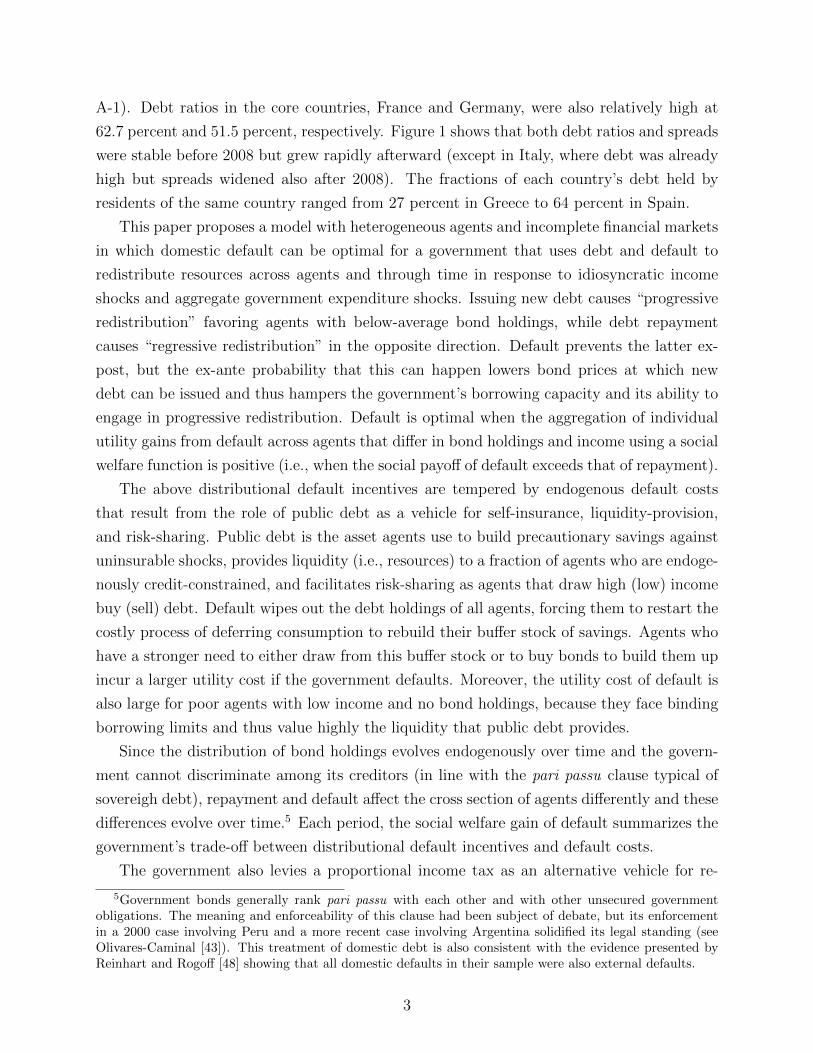
A-1). Debt ratios in the core countries, France and Germany, were also relatively high at

62.7 percent and 51.5 percent, respectively. Figure 1 shows that both debt ratios and spreads

were stable before 2008 but grew rapidly afterward (except in Italy, where debt was already

high but spreads widened also after 2008). The fractions of each country’s debt held by

residents of the same country ranged from 27 percent in Greece to 64 percent in Spain.

This paper proposes a model with heterogeneous agents and incomplete financial markets

in which domestic default can be optimal for a government that uses debt and default to

redistribute resources across agents and through time in response to idiosyncratic income

shocks and aggregate government expenditure shocks. Issuing new debt causes “progressive

redistribution” favoring agents with below-average bond holdings, while debt repayment

causes “regressive redistribution” in the opposite direction. Default prevents the latter ex-

post, but the ex-ante probability that this can happen lowers bond prices at which new

debt can be issued and thus hampers the government’s borrowing capacity and its ability to

engage in progressive redistribution. Default is optimal when the aggregation of individual

utility gains from default across agents that differ in bond holdings and income using a social

welfare function is positive (i.e., when the social payoff of default exceeds that of repayment).

The above distributional default incentives are tempered by endogenous default costs

that result from the role of public debt as a vehicle for self-insurance, liquidity-provision,

and risk-sharing. Public debt is the asset agents use to build precautionary savings against

uninsurable shocks, provides liquidity (i.e., resources) to a fraction of agents who are endoge-

nously credit-constrained, and facilitates risk-sharing as agents that draw high (low) income

buy (sell) debt. Default wipes out the debt holdings of all agents, forcing them to restart the

costly process of deferring consumption to rebuild their buffer stock of savings. Agents who

have a stronger need to either draw from this buffer stock or to buy bonds to build them up

incur a larger utility cost if the government defaults. Moreover, the utility cost of default is

also large for poor agents with low income and no bond holdings, because they face binding

borrowing limits and thus value highly the liquidity that public debt provides.

Since the distribution of bond holdings evolves endogenously over time and the govern-

ment cannot discriminate among its creditors (in line with the pari passu clause typical of

sovereigh debt), repayment and default affect the cross section of agents differently and these

differences evolve over time.5 Each period, the social welfare gain of default summarizes the

government’s trade-off between distributional default incentives and default costs.

The government also levies a proportional income tax as an alternative vehicle for re-

5Government bonds generally rank pari passu with each other and with other unsecured governmentobligations. The meaning and enforceability of this clause had been subject of debate, but its enforcementin a 2000 case involving Peru and a more recent case involving Argentina solidified its legal standing (seeOlivares-Caminal [43]). This treatment of domestic debt is also consistent with the evidence presented byReinhart and Rogoff [48] showing that all domestic defaults in their sample were also external defaults.

3

distribution that operates in the usual way to improve risk-sharing of idiosyncratic income

shocks. A 100 percent tax on individual income to finance a uniform lump-sum transfer

provides perfect risk-sharing of these shocks but still does not provide insurance against the

aggregate shocks. We study equilibria in which the income tax rate matches actual tax rate

estimates, which are well below 100 percent.

Foreign creditors also participate in the public debt market, so that we can study the

distribution of debt across domestic v. foreign creditors. These creditors are modeled as the

risk-neutral investors typical of the Eaton-Gersovitz [26] (EG hereafter) class of external de-

fault models, which yields the standard condition equating expected returns in government

debt with the world opportunity cost of funds, linking default risk premia to default prob-

abilities. As in EG models, we allow for the possibility that default imposes an exogenous

income cost. Default, debt, and risk premia dynamics, however, respond to very different

forces from those at work in EG models, because the government’s payoff function factors

in the utility of all domestic agents, including its creditors, and default has the endogenous

costs that result from impairing the use of debt for self-insurance, liquidity and risk-sharing.

A rich feedback mechanism connects the government’s debt issuance and default choices,

the price of government bonds, the optimal plans of individual agents, and the dynamics of

the distribution of bonds across agents. The latter are driven by the agents’ optimal plans

and determine the evolution of individual utility gains of default across the cross section of

agents. In turn, a key determinant of the agents’ plans is the default risk premium reflected

in the price of public debt, which is determined by the probability of default, which is itself

determined by the governments aggregation of the individual default gains.

Public debt, spreads, and the social welfare gain of default evolve over time driven by

this feedback mechanism as the exogenous shocks hit the economy. With low debt and/or

low government expenditures, repayment incentives are stronger producing “more negative”

welfare gains of default, which in turn make repayment and increased debt issuance optimal.

The balance changes at higher debt and/or higher government expenditures, and as the

dispersion of individual gains from default widens and the social welfare gain from default

rises, debt can reach levels at which default is optimal. In the baseline case, default wipes

out the debt and sets the economy back to a state in which repayment incentives are strong

because with zero debt the social value of debt is high. These dynamics also affect the

holdings of public debt by domestic and external agents. After a default, external debt rises

faster at first, as domestic demand grows gradually because of the utility cost of postponing

consumption to rebuild the buffer stock of savings, but over time, as domestic demand

continues to rise, domestic agents hold a larger share of public debt than foreign agents.

The optimal debt moves across three zones. First, a zone in which repayment incentives

4

are strong (i.e., the social gain of default is “very negative”), the optimal debt is sold at zero

default risk, and that debt is lower than that which maximizes the resources that can be

gained by borrowing. Second, a zone in which the optimal debt is still offered default-risk-

free but equals the amount of debt that yields the most resources possible. Here, weaker

repayment incentives result in bond prices that fall sharply if debt exceeds this amount, so

debt is sold at the risk-free price but constrained by the government’s inability to commit to

repay. Third, a zone in which repayment incentives are in between the first two cases, so that

the optimal debt carries default risk but still generates more resources than risk-free debt

and less than the maximum that could be gained with risky borrowing. In the first zone,

debt increases with government expenditures so as to serve the standard role of smoothing

lump-sum taxation, while in the other two the stronger default incentives make debt fall as

government expenditures rise.

We study the model’s quantitative predictions by solving numerically the recursive Markov

equilibrium without commitment using parameter values calibrated to the Eurozone. The

model supports equilibria with debt and default, and dynamics both over the long-run and

around default events are qualitatively in line with key features of the data. Comparing peak

values for high-default-risk events excluding default (since most Eurozone countries did not

default), the model approximates well the average total, domestic and external debt ratios,

and produces spreads even higher than in the data. In the long-run, the model matches the

ranking of the correlations of government expenditures with spreads, consumption, and net

exports. Matching these correlations is important because government expenditure shocks

(the model’s only aggregate shock) are central to the model’s feedback mechanism, since

these shocks weaken (strengthen) repayment incentives when they are high (low). The model

also nearly matches the relative variability of consumption and net exports, and produces

correlations with disposable income that have the same signs as in the data.

Defaults in the model have a low long-run frequency of 1.2 percent, very near the 1.1

percent unconditional frequency of domestic defaults in the Reinhart-Rogoff database. As in

the data, debt and spreads rise rapidly and suddenly in the periods close to a default, while

in earlier periods, debt is stable and sold at the risk-free price. External debt falls relative

to domestic debt as a default approaches, and is about 55 percent of total debt when default

hits. Thus, to an observer of the model’s time series, a debt crisis looks like a sudden shock

following a period of stability and with small variations in external debt. The debt buildup

coincides with relatively low government expenditures, which at first strengthen repayment

incentives and reduce the social welfare gain of default, but then as debt rises have the

opposite effects and yield rapidly rising spreads. Default occurs with a modest increase

in government purchases, which at the higher debt is enough to shift the distribution of

5

individual default gains to yield a positive social gain of default.

We use the model’s equilibrium recursive functions to show that there is significant dis-

persion in the effects of changes in debt and government expenditures on individual gains

from default across agents with different bond holdings and income. This dispersion reflects

differences in the agents’ valuation of the self-insurance, liquidity, and risk-sharing benefits

of debt, and also in the effect of the exogenous income shock of default. As a result of these

differences, the social distribution of default gains shifts markedly across states of debt and

government purchases, producing large shifts in the social welfare gain of default. The bond

pricing function has a shape similar to that in EG models: starting at the risk-free price when

debt is low and falling sharply as debt starts to carry default risk. The associated debt Laffer

curves shift downward and to the left at higher realizations of government expenditures and

display the three zones across which the optimal debt moves.

We conduct a sensitivity analysis to study the effects of changes in the social welfare

weights, the parameters that drive self-insurance incentives, the income tax rate, the exoge-

nous cost of default, and allowing for partial default. The quantitative results hinge on how

default incentives vary with each scenario, but in all scenarios the model sustains average

debt ratios comparable to those in the data and at a low but positive default frequency.

Spreads are large in most cases, except when the exogenous default cost is removed com-

pletely, but in this scenario the debt that can be sustained is still significantly constrained by

the government’s inability to commit. In this case, debt is optimally chosen to be risk-free

because otherwise bond prices drop too much, so that choosing risky debt generates fewer

borrowed resources.

This paper is part of the growing research programs on optimal debt and taxation in

incomplete markets models with heterogeneous-agents and on external sovereign default.

Well-known papers in the heterogeneous-agents literature explore the implications of public

debt in models in which debt provides similar benefits as in our model (e.g., Aiyagari and

McGrattan [6], Azzimonti et al. [11], Floden [27] and Heathcote [36]). Aiyagari and Mc-

Grattan [6] quantify the welfare effect of debt in a setup with capital and labor, distortionary

taxes, and an exogenous supply of debt. Calibrating the model to U.S. data and solving it

for a range of debt ratios, they found a maximum welfare gain of 0.1 percent. In contrast, a

variant of our model without default risk predicts that the gain of avoiding an unanticipated,

once-and-for-all default can reach 1.35 percent. Azzimonti et al. [11] link wealth inequality

and financial integration with the demand and supply for public debt to explain growing debt

ratios in the last decade. Heathcote [36] derives non-Ricardian implications from stochastic

proportional tax changes because of borrowing constraints. Floden [27] shows that transfers

rebating distortionary tax revenue dominate debt for risk-sharing of idiosyncratic risk. As

6

in this paper, these papers embody a mechanism that hinges on the variation across agents

in the benefits of public debt, but they differ from this paper in that they abstract from

sovereign default.

The recent literature on external default has made important contributions to the classic

EG model, following the early work by Aguiar and Gopinath [5], Arellano [8] and Yue [51].6

Of particular relevence for our analysis are studies dealing with tax and expenditure policies,

external debt denominated in domestic currency, and models of international coordination

(e.g., Cuadra et al. [20]), Dias et al. [22], and Du and Schreger [25]). The key difference

relative to our setup is that these studies assume a representative agent and do not focus on

default on domestic debt-holders. Other studies in this literature related to our work include

those focusing on the effects of default on domestic agents, foreign and domestic lenders,

optimal taxation, the role of secondary markets, discriminatory versus nondiscriminatory

default and bailouts (e.g., Guembel and Sussman [30]; Broner et al. [15]; Gennaioli et al.[29];

Aguiar and Amador [1]; Mengus [42]; Di Casola and Sichlimiris [23]; Perez [46]; Bocola [14];

Sosa Padilla [50]; and Paczos and Shakhnov [44]). As in some of these studies, default in

our setup is non discriminatory, but in general, these studies abstract from distributional

default incentives and social benefits of debt for self-insurance, liquidity and risk-sharing.

There is also a more recent literature in the intersection of heterogeneous-agents and

external default models. Bai and Zhang [12] study a model with a continuum of heteroge-

neous countries each facing a participation constraint. Our model differs in that we look at

a continuum of domestic heterogeneous agents with a single government, and we model the

default decision instead of a participation constraint. Dovis et al. [24] study distributional

incentives to default on external debt in a model with heterogeneous agents. Our work is

similar in that both models produce debt dynamics characterized by periods of sustained

increases followed by large reductions, and in both default has distributional incentives. The

two differ in that they focus on external default, and when they introduce uncertainty they

study equilibria without default spreads and assume complete markets, which alters the so-

cial value of debt. In addition, we conduct a quantitative analysis exploring the model’s

ability to explain the observed dynamics of debt and spreads. Aguiar et al. [3] study a setup

in which the heterogeneity is across country members of a monetary union, instead of across

agents inside a country. They show how lack of commitment and fiscal policy coordination

leads countries to overborrow due to a fiscal externality, focusing on public debt traded across

countries by risk-neutral investors, instead of default on risk-averse domestic debt holders.

Andreasen et al. [7] and Jeon and Kabukcuoglu [33] study models in which domestic income

heterogeneity plays a role in the determination of external defaults, and Arellano et.al. [9]

6Panizza et al. [45]; Aguiar and Amador [2]; and Aguiar et al. [4] survey the literature in detail.

7

and Rojas [49] study sovereign risk in models with heterogeneous firms.

The rest of this paper is organized as follows: Section 2 describes the model and defines

the recursive Markov equilibrium. Section 3 examines two variants of the model simplified to

highlight distributional default incentives (in a one-period setup without uncertainty) and the

social value of public debt (as the welfare cost of a surprise once-and-for-all default). Section

4 discusses the calibration procedure and examines the model’s quantitative implications.

Section 5 provides conclusions. An online Appendix provides details on the data, solution

method and additional features of the quantitative results.

2 A Bewley Model of Domestic & External Default

Consider an economy inhabited by a continuum of private agents with aggregate unit measure

and a benevolent government. There is also a pool of risk-neutral international investors that

face an opportunity cost of funds equal to an exogenous, world-determined real interest rate.

Domestic agents face two types of non insurable shocks: idiosyncratic income fluctuations and

aggregate shocks in the form of fluctuations in government expenditures and the possibility

of sovereign default. Asset markets are incomplete because the only available vehicle of

savings are one-period, non-state-contingent government bonds, which both domestic agents

and international investors can buy. The government also levies proportional income taxes,

pays lump-sum transfers, and chooses whether to repay its debt or not.

2.1 Private Agents

Agents have a standard constant relative risk aversion (CRRA) utility function:

U = E0

∞∑t=0

βtu(ct), u(ct) = c1−σt /(1− σ), (1)

where β ∈ (0, 1) is the discount factor, ct is individual consumption, and σ is the coefficient

of relative risk aversion.

Each period, an agent draws an idiosyncratic income realization from a discrete Markov

process with a bounded, non-negative set of realizations yt = y, . . . , y ∈ Y , and a transition

probability matrix defined as π(yt+1, yt), with stationary distribution π∗(y). These shocks

have zero mean across agents so that aggregate income is non-stochastic.

Agents can buy government bonds in the amount bt+1 ∈ B ≡ [0,∞). They cannot take

short positions, so they face the standard no-borrowing constraint bt+1 ≥ 0. The distribution

of agents over debt and income at date t is denoted as Γt(b, y).

If the government repays its outstanding debt, an individual agent’s budget constraint

8

at date t is:

ct + qtbt+1 = yt(1− τ y) + bt + τt. (2)

The right-hand side of this expression shows the after-tax resources available to the agent:

the agent’s income realization yt net of a proportional income tax levied at rate τ y, income

from the payout on individual debt holdings bt, and lump-sum transfers τt. This disposable

income pays for consumption and purchases of new government bonds bt+1 at the price qt.

Before writing the individual budget constraint for default states, we note two important

assumptions about default costs. First, the government re-enters the bond market in the

following period after a default. Hence, we relax the standard assumption of EG models

according to which one cost of default is exclusion from credit markets either forever or for

a stochastic number of periods. Second, we allow for the possibility that default imposes an

exogenous income cost akin to those widely used in the sovereign default literature. We use

it to construct a calibration comparable to those in the literature, and show later that the

model sustains debt even without it. In EG models, this cost is modeled as a function of the

realization of a stochastic endowment and designed so that default costs are higher at higher

income. Since aggregate income is constant in our setup, we model the cost as a function

of the realization of g instead. Aggregate income when a default occurs falls by the amount

φ(g), which is decreasing in g, so that that the default cost is higher when income is higher.

If the government defaults, an individual agent’s budget constraint is:

ct = yt(1− τ y)− φ(g) + τt. (3)

Three important effects of government default on households are implicit in this constraint:

(a) Bond holdings of all agents are wiped out, which hurts more agents with large bond

holdings; (b) the public debt market freezes, so that agents drawing high (low) income real-

izations cannot buy (sell) bonds for self-insurance, and public debt cannot provide liquidity

to credit-constrained agents; and (c) everyone’s income falls by φ(g).

2.2 Government

Each period, the government collects τ yY in income taxes, pays for gt, and, if it repays

outstanding debt Bt, it chooses the amount of new bonds to sell Bt+1 from the non-negative

set Bt+1 ∈ B ≡ [0,∞). The tax rate τ y is exogenous, constant, and strictly positive.

Government expenditures evolve according to a discrete Markov process with realization set

G ≡ g, . . . , g and associated transition probability matrix F (gt+1, gt).7 The processes for

7Nothing prevents consumption for agents with sufficiently low income from becoming nonpositive indefault states (i.e., ct = yt(1− τy)−φ(g)− gt+ τyY ≤ 0), although this does not happen in our quantitativeexercises. Ruling this out would require a restriction on the y and g processes to ensure positive consumption

9

y and g are assumed to be independent for simplicity.8 Lump-sum transfers are determined

endogenously as explained below, and their sign is not restricted, so τt < 0 represents lump-

sum taxes. As discussed in Heathcote et al. [38], affine tax functions, like the one used here,

approximate well actual tax and transfer programs. Notice also that τ yY is constant (since

both τ y and Y are constant), but individual income tax bills fluctuate with y.

The government has the option to default on Bt at each date t. The default choice

is denoted by the binary variable dt, with dt = 1 indicating default. The government’s

preferences are given by:

E0

∞∑t=0

βt∫B×Y

∑yi≤y

u(ct(bt, yt))dω(bt, yt). (4)

Hence, the government is a benevolent planner who maximizes a social welfare function that

aggregates the utility of agents who own bonds b and draw income y using the welfare weights

given by the function ω(b, y), which is defined as follows:

ω(b, y) =∑yi≤y

π∗(yi)(

1− e−bω

). (5)

In the y dimension, the weights match the long-run distribution of individual income π∗(y).

In the b dimension, the weights are given by an exponential function with scale parameter

ω, which we label “creditor bias,” because with a higher ω the government weights more

the utility of agents who hold larger bond positions. In the quantitative exercise, we first

calibrate these weights to match the mean spreads observed in the data, and then consider

variations of the ω(b, y) function, including a case in which we replace it with the average

distribution of bonds and income in the economy. Bhandari et. al. [13] and Chang et al.

[16] follow similar approaches of calibrating welfare weights to match data targets and using

also weights given by the long-run average of the model’s wealth distribution.

Bt+1 and τt are determined after the default decision. Lump-sum transfers are set as

needed to satisfy the government budget constraint. If the government repays, once the

debt is chosen, the government budget constraint implies:

τ d=0t = τ yY − gt −Bt + qtBt+1. (6)

If the government defaults, the current repayment is not made and new bonds cannot be

issued. Thus, default entails a one-period freeze of the public debt market. The government

at the lowest y for all g: g + τyY < (1− τy)y − φ(g).8The independence assumed here is between individual income and aggregate government expenditures.

10

budget constraint implies then:

τ d=1t = τ yY − gt. (7)

The above treatment of transfers is analogous to that in the EG models, except that in

EG models the resources generated by government debt (plus the primary surplus if any)

are transferred to a representative agent, instead of to a continuum of heterogeneous agents.

In the calibration, these transfers approximate a data average on welfare and entitlement

payments to individuals net of capital tax revenues, which are not modeled.

2.3 Foreign Investors

Foreign investors are modeled in the same way as in EG models: risk-neutral investors

with “deep pockets” who face an opportunity cost of funds r. Their holdings of domestic

government debt are denoted Bt+1, which is also the economy’s net foreign asset position

(NFA), and their expected profits are: Ωt = −qtBt+1+ (1−pt)(1+r)

Bt+1. In this expression, pt is the

probability of default at t+ 1 perceived as of date t, −qtBt+1 is the value of bond purchases

in real terms (i.e., the real resources lent out to the government at date t), and (1−pt)(1+r)

Bt+1 is

the expected present value of the debt payout at t+1, which occurs with probability (1−pt).Arbitrage implies that Ωt = 0, which yields this well-known no-arbitrage condition:

qt =(1− pt)(1 + r)

. (8)

2.4 Timing of transactions

The timing of decisions and market participation at any date t is as follows:

1. Date t begins. The values of y and g are realized.

2. Individual states b, y, the distribution Γt(b, y), and aggregate states B, g are

known, and income taxes are paid.

3. The government makes its optimal debt and default decisions, and agents make their

optimal plans.

• If the government repays, dt = 0, Bt is paid, the market of government bonds

opens, new debt Bt+1 is issued, lump-sum transfers are set according to equation

(6), private agents choose bt+1, and qt is determined.• If the government defaults, dt = 1, Bt and all domestic and foreign holdings of

government bonds are written off, the debt market closes, and lump-sum transfers

are set according to equation (7).

4. Agents consume, and date t ends.

11

2.5 Recursive Markov Equilibrium

We study a Recursive Markov Equilibrium (RME) in which the government chooses debt

and default optimally from a set of Conditional Recursive Markov Equilibria (CRME) that

represent optimal allocations and prices conditional on given debt and default choices. To

characterize these equilibria, we first rewrite the optimization problem of domestic agents

and the no-arbitrage condition of foreign investors in recursive form.

The aggregate state variables are B and g.9 The optimal debt issuance and default

decision rules are characterized by the recursive functions B′(B, g) and d(B, g) ∈ 0, 1,respectively.10 The probability of default at t+ 1 evaluated as of t, denoted p(B′, g), is:

p(B′, g) =∑g′

d(B′, g′)F (g′, g). (9)

The probability of defaulting at t+1 on an amount of debt B′ conditional on information

available at t is formed by adding up the transitional probabilities from g to g′ for which, at

the corresponding g′, the government would choose to default.

The state variables for an individual agent are the agent’s bond holdings and income

(b, y) and the aggregate states (B, g). Agents take as given d(B, g), B′(B, g), τ d=0(B, g),

and τ d=1(g), a bond pricing function q(B′, g), and the Markov processes of y and g. These

functions allow agents to project the evolution of aggregate states and bond prices, so that

an agent’s continuation value if the government has chosen to repay (d(B, g) = 0) and issued

B′(B, g) bonds can be represented as the solution to the following problem:

V d=0(b, y, B, g) = maxc≥0,b′≥0

u(c) + βE(y′,g′)|(y,g)[V (b′, y′, B′, g′)]

(10)

s.t.

c+ q(B′(B, g), g)b′ = b+ y(1− τ y) + τ d=0(B, g), (11)

where V (b′, y′, B′, g′) (without superscript) is the next period’s continuation value for the

agent before the default decision has been made that period.

Similarly, the continuation value if the government has chosen to default is:

V d=1(y, g) = u(y(1− τ y)− φ(g) + τ d=1(g)) + βE(y′,g′)|(y,g)[Vd=0(0, y′, 0, g′)]. (12)

9It is critical to note that Γt(b, y) is not a state variable despite the presence of aggregate risk. This isbecause it does not affect bond prices directly, since qt satisfies the foreign investors’ no-arbitrage condition,and the welfare weights are set by ω(b, y).

10In the recursive notation, variables xt and xt+1 are denoted as x and x′, respectively.

12

Finally, the continuation value at date t before the default decision is:

V (b, y, B, g) = (1− d(B, g))V d=0(b, y, B, g) + d(B, g)V d=1(y, g). (13)

The solution to this problem yields the individual decision rule b′ = h(b, y, B, g) and the

associated value functions V (b, y, B, g), V d=0(b, y, B, g) and V d=1(y, g). By combining the

agents’ bond decision rule, the Markov transition matrices of y and g, and the government’s

default decision, we can obtain expressions that characterize the evolution of the distribution

of bonds and income under repayment and default. The distribution at the beginning of t+1

is denoted Γ′ = Hd′∈0,1(Γ, B, g, g′). If d(B′, g′) = 0, for B0 ⊂ B, Y0 ⊂ Y , Γ′ is:

Γ′(B0,Y0) =

∫Y0,B0

∫Y,B

Ib′=h(b,y,B,g)∈B0π(y′, y)dΓ(b, y)db′dy′, (14)

where I· is an indicator function that equals 1 if b′ = h(b, y, B, g) and zero otherwise. Note

that g′ is an argument of Hd′∈0,1 because Γ′ is formed after d′ is known, and d′ depends on

g′. If d(B′, g′) = 1, for Y0 ⊂ Y , Γ′ is given by:

Γ′(0,Y0) =

∫Y0

∫Y,B

π(y′, y)dΓ(b, y)db′dy′, (15)

and zero otherwise. This is because at default all households’ bond positions are set to

zero, and hence Γ′ is determined only by the evolution of the income process (i.e., if the

government defaults, Γ′(b, y) = π∗(y) for b = 0 and zero for any other value of b).

The recursive form of the foreign investors’ no-arbitrage condition is:

q(B′, g) =(1− p(B′, g))

(1 + r). (16)

The wedge between the price at which foreign investors are willing to buy sovereign debt

(q(·)) and the price of international bonds (1/(1 + r)) compensates them for the risk of de-

fault measured by the default probability. At equilibrium, bond prices and risk premia are

formed by a combination of exogenous factors (the Markov process of g) and the endogenous

government decision rules B′(B, g) and d(B, g). Despite the similarity with the debt pric-

ing condition of EG models, however, the mechanism determining default probabilities and

default risk is very different. In EG models, these probabilities follow from the values of con-

tinuation v. default of a representative agent, which exclude the welfare of the government’s

creditors. In this model, default probabilities are determined by comparing continuation v.

default values for the social welfare function, which include the welfare of domestic creditors

and depend on the dispersion of individual payoffs of default v. repayment. Hence, inequal-

13

ity affects default risk via changes in the dispersion of these payoffs. Later in this Section, we

characterize the mechanism driving the dispersion in payoffs, and in Section 4 we illustrate

it quantitatively.

Using the foreign lenders’ no-arbitrage condition to price the debt implies that they are

the marginal buyer. This assumption is valid if at that price B′ ≥ 0, indicating that domestic

demand for public debt is smaller than the supply the government issues, which makes NFA

negative (i.e. the country is a net external borrower). Hence, at the no-arbitrage price foreign

lenders are indifferent between the sovereign bond and the world asset that pays r. Relative

to that price, for a given (B′, g) and abstracting from changes in future default incentives, a

lower price results in excess demand for sovereign debt (since foreign and domestic demand

increase) and a higher price results in excess supply (since foreign and domestic demand

decrease). This assumption is validated quantitatively, because in the experiments with the

baseline calibration and several variants B′ ≥ 0 in all periods along the equilibrium path.11

We now define the CRME for given debt and default decision rules. The definition

includes the following three aggregate variables. First, aggregate consumption is given by:

C =

∫Y×B

c(b, y, B, g) dΓ(b, y), (17)

where c(b, y, B, g) corresponds to individual consumption by each agent. Second, aggregate

(nonstochastic) income is:

Y =

∫Y×B

y dΓ(b, y). (18)

Third, aggregate domestic demand for newly issued bonds is:

Bd′ =

∫Y×B

h(b, y, B, g) dΓ(b, y). (19)

Definition: Given an initial distribution Γ0(b, y), a default decision rule d(B, g), a gov-

ernment debt decision rule B′(B, g), an income tax rate τ y, and lump-sum transfers τ d∈0,1

defined by (6) and (7), a CRME is defined by a value function V (b, y, B, g) with associated

household decision rule b′ = h(b, y, B, g), a transition function for the distribution of bonds

and income Hd′∈0,1(B, g, g′), a default probability function p(B′, g), and a bond pricing

function q(B′, g) such that:

1. Given the q(B′, g) and government policies, V (b, y, B, g) and h(b, y, B, g) solve the

individual agents’ optimization problem.

11The solution algorithm assumes that if B′ < 0 domestic agents buy foreign bonds at the price 1/(1 + r)for the amount by which their demand exceeds the bonds sold by the government, and NFA becomes positive.Quantitatively, this only happens in one of the sensitivity experiments with a high CRRA coefficient.

14

2. The foreign investors’ arbitrage condition (equation (16)) holds.

3. The transition function of the distribution of bonds and income satisfies conditions

(14) and (15) in states with repayment and default, respectively.

4. The government budget constraints (6) and (7) hold.

5. The market of government bonds clears: B′ +Bd′ = B′.

6. The aggregate resource constraint of the economy is satisfied. If the government repays:

C + g = Y + B − q(B′, g)B′, and if the government defaults: C + g = Y − φ(g).

The model’s RME is defined as a CRME in which B′(B, g) and d(B, g) are optimal

government choices. If B > 0 at the beginning of period t, the government sets its optimal

d(B, g) as the solution to the following problem:

maxd∈0,1

W d=0(B, g),W d=1(g)

, (20)

where the social value of continuation is:

W d=0(B, g) =

∫Y×B

V d=0(b, y, B, g)dω(b, y),

and the social value of default is:

W d=1(g) =

∫Y×B

V d=1(y, g)dω(b, y).

If the government chooses to repay, it also chooses an optimal amount of new debt to issue.

To characterize this choice, assume that the government first considers an intermediate step

in which it evaluates how any arbitrary debt level (denoted B′) affects individual agents. The

corresponding value for an agent with a (b, y) pair is the solution to the following problem:

V (b, y, B, g, B′) = maxc≥0,b′≥0

u(c) + βE(y′,g′)|(y,g)[V (b′, y′, B′, g′)] (21)

s.t.

c+ q(B′, g)b′ = y(1− τ y) + b+ τ

τ = τ yY − g −B + q(B′, g)B′.

Note that V (·) in the right-hand side of this problem is given by the solution to the agents’

problem (10), which implies that the government is assessing the lifetime utility effect of

deviating from the optimal policy only in the current period. The optimal debt issuance

decision rule then solves this problem:

maxB′

∫Y×B

V (b, y, B, g, B′)dω(b, y). (22)

15

Now we can define the model’s RME:

Definition: A RME is a CRME in which the default decision rule d(B, g) solves problem

(20) and the debt decision rule B′(B, g) solves problem (22).

2.6 Optimality Conditions & Feedback Mechanism

We discuss next key features of the model’s optimality conditions that illustrate the feedback

mechanism linking default incentives, default risk, the distribution of bond holding, and the

dispersion of individual gains from a default. This material will also be used for the analysis

of the quantitative results in Section 4.

(a) Default risk and demand for government bonds.

Assuming the agents’ value functions are differentiable, the first-order condition for b′ in

a state in which the government has repaid is:

−u′(c)q(B′, g) + βE(y′,g′)|(y,g) [V1(b′, y′, B′, g′)] ≤ 0, = 0 if b′ > 0, (23)

where V1(·) denotes the derivative of V (·) with respect to its first argument. Using the

envelope theorem, this condition can be rewritten as:

u′(c) ≤ βE(y′,g′)|(y,g)

[(1− d(B′, g′))

u′(c′)

q(B′, g)

], (24)

which holds with equality if b′ > 0. The right-hand-side of this expression shows that, in

assessing the marginal benefit of buying an extra unit of b′, agents take into account the

possibility of a future default. In states in which a default is expected, d(B′, g′) = 1 and

agents assign zero marginal benefit to buying bonds.12 In states in which repayment is

expected, the marginal benefit of buying bonds is u′(c′)q(B′,g)

, which includes the default risk

premium embedded in the price paid for newly issued bonds.

These results imply that, conditional on B′, a larger default set (i.e., a larger set of values

of g′ for which the government defaults) reduces the expected marginal benefit of an extra

unit of b′. In turn, this implies that, everything else equal, a higher default probability

reduces individual domestic demand for government bonds unless an agent has high enough

(b, y) to be willing to take the risk of demanding more bonds at higher risk premia (lower bond

prices) and expect future adjustments in τ . This has important distributional implications

because, as we explain below, the government internalizes when making the default decision

how it affects the probability of default and bond prices. Notice also that future default risk

at any date later than t, not just t+ 1, influences the agents’ demand for bt+1 because of the

12In the next Section, we solve also variants of the model that allow for partial defaults, in which themarginal benefit of buying bonds in the default state is positive, instead of zero.

16

time-recursive structure of Euler equation (24). Hence, even if debt is offered at the risk-

free price at t, bond demand still responds negatively to default risk if default has positive

probability beyond t + 1 (i.e., agents factor in the risk of a future default wiping out their

wealth as they build their individual stock of savings).

(b) Self-insurance, liquidity, and risk-sharing roles of public debt

The roles of public debt as a vehicle for self-insurance, liquidity, and risk-sharing can be

illustrated by combining the agents’ budget constraint with the government budget constraint

using the variable transformation b = (b−B) to obtain:

c = y + b− q(B′, g)b′ − τ y(y − Y )− g (25)

b′ ≥ −B′ (26)

The liquidity benefit of public debt is evident in condition (26): Selling new debt (B′)

relaxes the borrowing constraint for agents for whom it is binding. That is, it provides them

with liquidity in the form of extra resources for consumption. The self-insurance role can be

inferred from condition (25): Agents who draw sufficiently high y, regardless of their existing

holdings of b, want to buy more debt, and agents who draw sufficiently low y want to draw

from their accumulated precautionary savings. The risk-sharing benefit is also reflected in

condition (25): by buying (selling) debt, agents drawing high (low) income share the risk of

idiosyncratic income fluctuations with each other, albeit imperfectly.

The role of income taxation as an alternative means to improve risk-sharing of idiosyn-

cratic income shocks is also evident in condition (25): The term −τ y(y − Y ) implies that

agents with below (above) average income effectively receive (pay) a subsidy (tax). If income

is taxed 100 percent, full social insurance against these shocks is provided (i.e. perfect risk

sharing), and all agents after-tax income equals Y . But this still would not remove the need

for precautionary savings, because aggregate shocks to government expenditures as well as

government defaults cannot be insured away.

In making its debt and default choices, the government trades off the above social benefits

of debt v. the distributional implications of debt repayment and issuance. At any date t,

repayment of B results in regressive redistribution in favor of agents with sufficiently large

holdings of the outstanding public debt (i.e., agents with b > 0, or “above average” holdings

relative to B). In contrast, issuing new debt B′ causes progressive redistribution in favor of

agents who buy sufficiently little or no new debt (i.e., agents with b′ < 0, or below average

holdings relative toB′). The magnitude and cross-sectional dispersion of these effects changes

over time as the endogenous distribution of bond holdings evolves.

The two forms of redistribution are connected inter-temporally. Under repayment, more

progressive redistribution at t implies more regressive redistribution in the future. Because

17

of the government’s inability to commit to repay, however, the extent to which progressive

redistribution can be implemented at t is inversely related to the expectation that in the

future the planner may wish to avoid regressive redistribution by defaulting. This is because

the price at which new debt is sold at t depends negatively on the probability of a default at

t+ 1. This weakens the government’s ability to produce progressive redistribution, because

q(B′, g) falls as B′ rises, since the default probability is nondecreasing in B′. Hence, the

resources generated by debt, q(B′, g)B′, follow a Laffer curve similar to the familiar one

from EG models, because in those models bond prices also fall and default probabilities also

rise as debt rises. In EG models, however, the resources generated by debt are transferred to

a representative agent, while here they are transferred to heterogeneous agents, and although

τ is uniform across agents, the heterogeneity in bond holdings makes the transfers generated

by debt vary across agents (inversely with the value of b′).

(c) Feedback mechanism

The feedback mechanism driving the model follows from the features highlighted in (a)

and (b). In particular, it is critical to note that the probability of default and the price of

debt at t depend on the dispersion of payoffs of default versus repayment across agents at

t+ 1, because the government’s social welfare function aggregates these payoffs to make the

default decision. This is a feedback mechanism because the debt issued at t becomes the

initial debt outstanding at t + 1 and this matters for the dispersion of the agents’ payoffs,

affecting agents with different (b, y) differently, as we illustrate quantitatively in Section

4. Thus, the debt issued at t affects the default decision at t + 1, which affects default

probabilities and bond prices at t, which in turn affects the agents’ date-t demand for bonds

and the government’s debt choice. The links of this chain are connected via the distributional

effects of debt issuance, the social benefits of debt, and the dispersion of payoffs of default

versus repayment across agents.

This feedback mechanism cannot be fully characterized analytically in closed form, but

we can gain further intuition about it as follows. Define ∆c ≡ cd=0 − cd=1 as the difference

in consumption across repayment and default in a given period for an agent who has a

particular b when the aggregate states are (B, g). ∆c can be expressed as:

∆c = b− q(B′, g)b′ + φ(g) (27)

The right-hand-side of this expression includes the distributional effects noted in (b). If

inequality in the initial distribution of government debt is high, so that a larger fraction

of agents have b < 0, and strong default incentives make default risk high, so that q(B′, g)

is low, a larger fraction of agents have ∆c < 0 and are more likely to be better off with

a default, which in turn justifies the distributional incentives to default. The opposite is

18

true if initial inequality in bond holdings and default risk are low. Moreover, given initial

inequality and bond prices, higher inequality in the end-of-period distribution of government

debt (i.e., a larger fraction of agents with b′ < 0) reduces the fraction of agents with ∆c < 0.

Hence, changes in the distribution of public debt, default incentives, and default risk interact

in determining the dispersion of ∆c < 0 across agents. The interaction does not follow a

monotonic pattern, however, because ∆c can be negative also for agents with sufficiently

high (b, y) who buy more risky debt attracted by the higher risk premia. Thus, as we look

across agents with different bond holdings, db′

dBchanges sign and, for some large bond holders

it can even be the case that ∆c decreases with B.

It is also important to note that ∆c alone does not determine individual payoffs of

default or repayment. These depend on both date-t differences in consumption (or utility)

and differences in the continuation values V d=0(b′, y′, B′, g′) and V d=0(0, y′, 0, g′). Still, the

interaction between the distribution of government debt, consumption differentials across

default and repayment states, and default risk discussed previously is illustrative of the

feedback mechanism driving the model. Moreover, we can also establish that, since V d=0

is increasing in b as in standard heterogeneous-agents models, there is a threshold value of

bond holdings b(y,B, g), for given (y,B, g), such that agents with b ≥ b prefer repayment

(since V d=0(b, y, B, g) ≥ V d=1(y, g)), and those with b < b(y,B, g) prefer default. That is,

b(y,B, g) = b ∈ B : V d=0(b, y, B, g) = V d=1(y, g). (28)

We can conjecture that b(y,B, g) is increasing in B because the difference in τ under repay-

ment v. default widens at higher debt: Higher debt reduces transfers both because of the

higher repayment on B even without default risk and because higher risk premia reduces

the price at which Bt+1 is sold, causing a debt-overhang effect (i.e., additional borrowing is

used to service debt). As a result, agents need to have higher individual wealth in order to

prefer repayment as B rises. This conjecture was verified numerically in Appendix A-6.

3 Distributional Incentives & Social Value of Debt

This Section examines two simplified versions of the model. First, a one-period variant

designed to isolate the distributional default incentives. By construction, this setup abstracts

from the social benefits of debt for self-insurance, liquidity, and risk-sharing. The second

variant isolates these social benefits by quantifying the welfare costs of a once-and-for-all

default. The quantitative analysis of the full model in the next Section combines the elements

isolated in these exercises.

19

3.1 Distributional default incentives

Consider a one-period variant of the model without uncertainty and a predetermined distri-

bution of debt ownership. There are two types of agents: A fraction γ are L−type agents

with low bond holdings denoted bL, and the complement (1 − γ) are H−type agents with

high bond holdings bH . The government has an exogenous stock of debt B, which is deciding

whether to repay or not, and default may entail an exogenous cost that reduces income by

a fraction φ ≥ 0. We include this cost because, as we show below, distributional incentives

alone cannot sustain debt in this simple model unless the social welfare function weights L

types by less than γ. This cost can proxy for the endogenous default costs driven by the

social value of debt in the full model.

The budget constraints of the government and households under repayment are τ d=0 =

B−g and ci = y+τ d=0 +bi (for i = L,H), respectively, and under default are τ d=1 = −g and

ci = (1− φ)y+ τ d=1 (for i = L,H), respectively. The utility function can be as in Section 2,

but what is necessary for the results derived here is that it be increasing and strictly concave.

Since there is only one period, the agents’ choices of bL and bH (or equivalently their

consumption allocations) are predetermined. In particular, we consider a given exogenous

“decentralized” distribution of debt holdings characterized by a parameter ε, so that the

bond holdings of L-types are bL = B − ε and then market-clearing in the bond market

requires bH = B + γ1−γ ε. We are still assuming agents cannot borrow, so it must be that

ε ≤ B, and since by definition bH ≥ bL, it must be that ε ≥ 0. Using the budget constraints,

the decentralized consumption allocations under repayment and default are cL(ε) = y−g− εand cH(γ, ε) = y − g + γ

1−γ ε and cL = cH = y(1 − φ) − g, respectively. Notice that under

repayment, ε determines also the dispersion of consumption across agents, which increases

with ε, and under default there is zero consumption dispersion.

The main question to understand distributional incentives to default is: How does an

arbitrary distribution of bond holdings (or dispersion of consumption) defined by ε differ

from the one that is optimal for a government with the option to default? To answer this

question, we solve the optimization problem of the social planner with the default option.

The planner’s welfare weight on L-type agents is ω. The optimal default decision solves:

maxd∈0,1

W d=0

1 (ε),W d=11 (φ)

, (29)

where social welfare under repayment is:

W d=0(ε) = ωu(y − g + ε) + (1− ω)u

(y − g +

γ

1− γε

)(30)

20

and under default is:

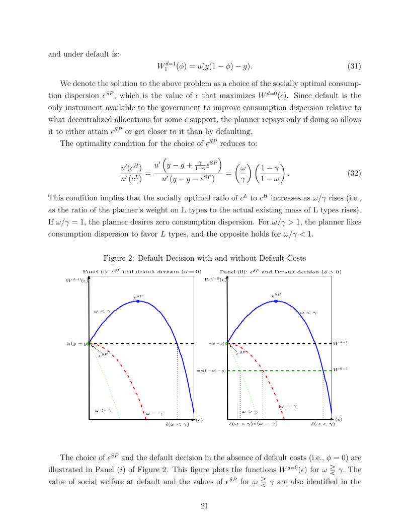
W d=11 (φ) = u(y(1− φ)− g). (31)

We denote the solution to the above problem as a choice of the socially optimal consump-

tion dispersion εSP , which is the value of ε that maximizes W d=0(ε). Since default is the

only instrument available to the government to improve consumption dispersion relative to

what decentralized allocations for some ε support, the planner repays only if doing so allows

it to either attain εSP or get closer to it than by defaulting.

The optimality condition for the choice of εSP reduces to:

u′(cH)

u′ (cL)=u′(y − g + γ

1−γ εSP)

u′ (y − g − εSP )=

(ω

γ

)(1− γ1− ω

). (32)

This condition implies that the socially optimal ratio of cL to cH increases as ω/γ rises (i.e.,

as the ratio of the planner’s weight on L types to the actual existing mass of L types rises).

If ω/γ = 1, the planner desires zero consumption dispersion. For ω/γ > 1, the planner likes

consumption dispersion to favor L types, and the opposite holds for ω/γ < 1.

Figure 2: Default Decision with and without Default Costs

Panel (i): ǫSP and default decision (φ = 0)

(ǫ)

W d=0(ǫ)

ǫSP

ǫ(ω < γ)

ǫSP

ω < γ

ω = γω > γ

u(y − g)

(ǫ)

W d=0(ǫ)

Panel (ii): ǫSP and Default decision (φ > 0)

ǫ(ω < γ)ǫ(ω > γ)

ω < γ

ω = γ

ω > γ

u(y− g)

u(y(1 − φ)− g)

ǫSP

ǫ(ω = γ)

ǫSP

W d=1

W d=1

The choice of εSP and the default decision in the absence of default costs (i.e., φ = 0) are

illustrated in Panel (i) of Figure 2. This figure plots the functions W d=0(ε) for ω R γ. The

value of social welfare at default and the values of εSP for ω R γ are also identified in the

21

plot. Notice that the vertical intercept of W d=0(ε) is always W d=1 for any values of ω and γ

because, when ε = 0, there is zero consumption dispersion and that is also the outcome under

default. In addition, the bell-shaped form of W d=0(ε) follows from u′(·) > 0, u′′(·) < 0.13

Assume first that ω > γ. In this case, εSP would be negative because condition (32)

implies that the planner’s optimal choice features cL > cH . However, these consumption

allocations are not feasible (since they imply ε < 0), and by choosing default the government

attains W d=1, which is the highest feasible social welfare for ε ≥ 0. Assuming instead ω = γ,

it follows that εSP = 0 and default attains exactly that same level of welfare, so default is

chosen and it also delivers the efficient level of consumption dispersion. In short, if ω ≥ γ,

the government always defaults for any ε > 0, and thus equilibria with debt cannot be

supported. Intuitively, the consumption allocations feature cH > cL for any ε > 0, while the

socially efficient consumption dispersion requires cH ≤ cL, and thus default is a second-best

policy that brings the planner the closest it can get to εSP (since the only instrument for

redistribution is the default choice).

Equilibria with debt can be supported when ω < γ. The intersection of the downward-

sloping segment of W d=0(ε) with W d=1 determines a threshold value ε such that default is

optimal only for ε ≥ ε. Default is still a second-best policy because with it the planner cannot

attain W d=0(εSP ), it just gets the closest it can get. As Figure 2 shows, for ε < ε, repayment

is preferable because W d=0(ε) > W d=1. Thus, in this simple setup and when default is

costless, equilibria with repayment require two conditions: (a) that the government weights

H types by more than their share of the government bond holdings and (b) that the debt

holdings of private agents do not produce consumption dispersion in excess of ε.

Add now the exogenous cost of default. The solutions are shown in Panel (ii) of Figure

2. The key difference is that now it is possible to support repayment equilibria even when

ω ≥ γ. There is a threshold value of consumption dispersion, ε, separating repayment from

default decisions for all values of ω and γ. The government chooses to repay whenever ε

exceeds ε for the corresponding values of ω and γ. It is also evident that the range of values

of ε for which repayment is chosen widens as γ rises relative to ω. Thus, when default is costly,

equilibria with repayment require only that the debt holdings of private agents implicit in

ε do not produce consumption dispersion in excess of the value of ε associated with given

values of ω and γ. Intuitively, the consumption of H type agents must not exceed that of L

type agents by more than what ε allows. If it does, default is optimal.

D’Erasmo and Mendoza [21] extend this analysis to a two-period model with shocks

13Note in particular that ∂Wd=0(ε)∂ε R 0 ⇐⇒ u′(cH(ε))

u′(cL(ε))R (ωγ )( 1−γ

1−ω ). Hence, social welfare is increasing

(decreasing) at values of ε that support sufficiently low (high) consumption dispersion so that u′(cH(ε))u′(cL(ε))

is

above (below) (ωγ )( 1−γ1−ω ).

22

to government expenditures, optimal bond demand choices by private agents, and optimal

bond supply and default choices by the government. The results for the distributional default

incentives derived above still hold. In addition, we show that the optimal debt and default

choices are characterized by a socially optimal deviation from the equalization of marginal

utilities across agents, which calls for higher debt the higher the liquidity benefit of debt

in the first period (i.e., the tighter the credit constraint on L-types) and the higher the

marginal distributional benefit of a default in the second period. We also show that the

model still sustains debt with default risk if we introduce a consumption tax as a second

tool for redistribution, an alternative asset for savings, and foreign creditors.

3.2 Social Value of Debt

We conduct now a quantitative exercise that measures the endogenous costs of default cap-

tured by the social value of debt. In particular, we compute the social cost of a once-and-

for-all, unanticipated default, which captures the costs of wiping the buffer stock of savings

of private agents, preventing debt issuance from providing liquidity to credit-constrained

agents, and precluding purchases (sales) of government bonds from improving risk-sharing.

The goal is to show that default in the model of Section 2 can yield large endogenous costs.

To quantify the social cost of a once-and-for-all, unanticipated default, we compare social

welfare across two economies. As in the full model, these economies are inhabited by a

continuum of heterogeneous agents facing idiosyncratic (income) and aggregate (government

expenditure) shocks. In the first economy, the government is fully committed to repay, while

in the second there is an exogenous once-and-for-all, unanticipated default in the first period

(i.e., a “surprise” default). After that, the government is committed to repay. We perform

the experiment for different initial levels of government debt. Since there is no default risk,

bond prices are always equal to 1/(1 + r) and the domestic aggregate demand for bonds is

the same for the different values of B (what changes is the amount traded abroad).

This experiment is related to the one conducted by Aiyagari and McGrattan [6], but

with important differences. First, we compute the cost of a surprise default relative to an

economy with full commitment, whereas they calculate the cost of changing the debt ratio

under full commitment. Second, their model features production and capital accumulation

with distortionary taxes, which we abstract from, but considers only idiosyncratic shocks,

while we incorporate aggregate shocks. Third, in our setup, the interest rate is always

1/(1 + r), whereas they study a closed economy with an endogenous interest rate.

We quantify the social value of public debt as the welfare cost computed as follows:

Define α(b, y, B, g) as the individual welfare effect of the surprise default. This corresponds

to a compensating variation in consumption such that, at a given aggregate state (B, g), an

agent with a (b, y) pair is indifferent between living in the economy in which the government

23

always repays and the one with the surprise default.14 Formally, α(b, y, B, g) is given by:

α(b, y, B, g) =

[V d=1(y, g)

V c(b, y, B, g)

] 11−σ

− 1,

where V d=1(y, g) represents the value of the surprise default, and V c(b, y, B, g) is the value

under full commitment. For a given (B, g), there is a distribution of these individual welfare

measures across all the agents defined by all (b, y) pairs in the state space. The social value

of public debt is then computed by aggregating these individual welfare measures using the

social welfare function defined in Section 2:

α(B, g) =

∫α(b, y, B, g)dω(b, y). (33)

Table 1 shows results for four scenarios corresponding to surprise defaults with debt ratios

ranging from 5 to 20 percent of GDP.15

Table 1: Social Value of Public Debt

Panel (a): Calibrated welfare weightsB/GDP Bd/GDP τ(B, µg)/GDP α(B, µg)% α(B, g) α(B, g) hh’s α(b, y, B, µg) > 0

5.0 4.25 25.96 -1.87 -4.66 -1.13 0.910.0 4.25 23.87 -0.90 -3.76 -0.12 29.115.0 4.25 20.83 0.04 -2.88 0.89 66.020.0 4.25 17.29 1.00 -1.99 1.90 83.9

Panel (b): Welfare weights set to mean wealth distributionB/GDP Bd/GDP τ(B, µg)/GDP α(B, µg)% α(B, g) α(B, g) hh’s α(b, y, B, µg) > 0

5.0 4.25 27.16 -1.75 -4.56 -1.00 0.010.0 4.25 25.22 -0.95 -3.81 -0.15 9.215.0 4.25 22.74 0.00 -2.93 0.85 75.820.0 4.25 19.73 1.07 -1.92 1.99 86.9

Note: Values are reported in percentage. Bd/GDP corresponds to the average of 10,000-period simulationswith the first 2,000 periods truncated. Positive values of α(B, g) denote that social welfare is higher in theonce-and-for-all default scenario than under full repayment commitment. “hh’s” denotes households.

For each scenario, Table 1 shows GDP ratios of total public debt, B/GDP , domestic

debt, Bd/GDP , transfers τ (evaluated at average g = µg and the corresponding level of

14We measure welfare relative to this scenario, instead of permanent financial autarky, because it is in linewith the one-period debt-market freeze when default occurs in our model. The costs relative to full financialautarky would be larger but less representative of the model’s endogenous default costs.

15We use the parameters from the calibration described in the next Section and listed in Table 2.

24

B), as well as α(B, g) for different values of g (average µg, minimum, g, and maximum,

g). We also report the fraction of agents with α(b, y, B, µg) > 0 (i.e., the fraction of agents

benefiting from a default). Since computing Bd requires the distribution Γ(b, y), we report

Bd for a “panel average,” calculated by first averaging over the cross-section of (b, y) pairs

within each period, and then averaging across a long time-series simulation. We show results

for two sets of welfare weights. Panel (a) uses the ω(b, y) function defined earlier using the

parameterization from the baseline calibration of the next Section. Panel (b) defines ω(b, y)

as the long-run average of the distributions of bond and income obtained by solving the

model without default risk, denoted Γrf (b, y).

The results show that the social value of debt is large and decreases monotonically as

debt rises. For g = µg, the results range from a social cost of -1.87 percent for defaulting on

a 5 percent debt ratio to a gain of 1.00 for defaulting on a 20 percent debt ratio (i.e. the

social value of debt ranges from 1.87 to -1.00 percent). Surprise defaults are very costly for

debt ratios of 10 percent or less, while they yield welfare gains at debt ratios of 15 percent

or higher. For the low value of g, default remains significantly costly even at a 20 percent

debt ratio. Interestingly, at the high value of g the welfare costs are smaller and the gains

larger than for average g, and they change from costs to gains at a debt ratio between 10 and

15 percent. These estimates of the social value of debt are significantly larger than those

obtained by Aiyagari and McGrattan [6], who reported the largest estimate of the social

value of debt at about 0.1 percent, while we obtain 1.87 percent (for g = µg). Moreover,

our estimates do not vary much if we change the calibrated welfare weights for weights that

match the long-run endogenous distribution of bonds and income of the economy without

default risk (see Panel (b)).

The smaller social value of debt (higher social value of default) at higher debt ratios

follows from the fact that higher debt reduces transfers (τ decreases monotonically) and

thus limits the extent to which the government can redistribute resources across agents

by repaying, while the benefits of debt for self-insurance, liquidity, and risk-sharing fall.

Accordingly, the fraction of agents that favor a default on average increases monotonically

with the debt ratio. At relatively low debt (below 10 percent of GDP) only up to 30 percent

of the population favors a default. These are agents with relatively low bond holdings who

benefit from a smaller cut in transfers after a government default. The larger cut in transfers

due to higher debt service when debt increases beyond 10 percent of GDP induces even agents

with sizable bond holdings to favor default. For instance, with a 20 percent debt ratio, the

average fraction of agents in favor of default is roughly 83.9 percent.

25

4 Quantitative Analysis

In this Section, we study the model’s quantitative predictions. The Section begins with the

calibration to Eurozone data, followed by an analysis of time-series properties, equilibrium

recursive functions, and a sensitivity analysis. The solution algorithm solves the RME using a

backward-recursive strategy over a finite horizon of arbitrary length until the value functions,

decision rules, and bond pricing function converge (see Appendix A-3 for details).16

4.1 Calibration

We calibrate the model to the Eurozone following our motivation to view the European debt

crisis as a domestic debt crisis, in which European institutions internalized the tradeoffs be-

tween distributional effects of individual country defaults and their implications for financial

markets across the region.17 During this crisis, default risk rose sharply for several Eurozone

countries and one them defaulted (Greece). The model is calibrated at an annual frequency

targeting GDP-weighted averages of country-specific moments. Hence, the calibration tar-

gets combine countries at the center of the crisis (e.g. Spain, Greece) with others that were

less affected (e.g. France, Netherlands).18 The parameter values that need to be set are

the subjective discount factor (β), the coefficient of relative risk aversion (σ), the moments

of the processes of individual income (µy, ρy, σu) and government expenditures (µg, ρg, σe),

the income tax rate (τ y), the opportunity cost of foreign investors (r), the parameters that

define φ(g), and the creditor bias parameter (ω).

The Markov processes of y and g approximate log-AR(1) time-series processes:

log(yt+1) = (1− ρy) log(µy) + ρy log(yt) + ut, (34)

log(gt+1) = (1− ρg) log(µg) + ρg log(gt) + et, (35)

where |ρy| < 1, |ρg| < 1 and ut and et are i.i.d. normal errors with zero means and standard

deviations σu and σe, respectively. These moments are calibrated to data following the

procedure we describe below. The Markov representation is constructed using Tauchen’s

quadrature method, set to produce grids with 5 evenly-spaced nodes for y and 25 for g,

centered at the means, and with the lowest and highest nodes set at plus and minus 2.5

standard deviations from the mean in logs. The variances of the Markov processes are

16The algorithm is similar to the one in Corbae et al. [19], who examined a heterogeneous-agents modelwith a feedback mechanism connecting wealth dynamics and optimal policies but without debt and default.

17We use data for Austria, Belgium, Finland, France, Germany, Greece, Ireland, Italy, Netherlands, Por-tugal, and Spain. See Appendix A-2 for a description of the data, sources, and country-specific moments.

18We also conducted the same set of experiments documented in this Section using a calibration based ondata for Spain only. The results are available in Appendix A-8.

26

within 1 percent of their AR(1) counterparts.

The parameter values are assigned in two steps. First, the values of all parameters except

β, ω and the function φ(g) are set to values commonly used in the literature or to estimates

obtained from the data. Second, β, ω and φ(g) are calibrated using the Simulated Method

of Moments (SMM) to minimize the distance between target moments from the data and

their model counterparts. Thus, these parameters are set by solving the model repeatedly

until the SMM converges, conditional on the parameter values set in the first step. We use

data from several sources. The sample period for most variables is 1981−2015. Appendix

A-2 provides a detailed description of the data and related transformations.

The first step of the calibration proceeds as follows: We set σ = 1 (i.e. log utility), which

is in the range commonly used in macro models. The risk-free interest rate is set to r = 0.013,

which is the average annual real return on German EMU-convergence criterion government

bonds in the European Commission’s Eurostat database for the period 2002−2015 (these

are secondary market returns, gross of tax, with around 10 years’ residual maturity). We

start in 2002, the year the euro was introduced, to isolate spreads from currency risk.

Comprehensive disaggregated panel datasets on individual earnings with sufficient detail

to estimate the persistence of the y process are unavailable, so we set ρy = 0.85 which is a

standard value in the heterogeneous-agents literature derived from U.S. data (e.g., Guvenen

[31]).19 For the variance of earnings, we use Var(log(y)) = 0.30, which is close to the midpoint

of estimates of the residual cross-sectional variance of log-earnings for Italy, Germany, and

Spain, which range from 0.2 to 0.55 (see Fuchs-Schundeln et al. [28] for Germany, Japelli and

Pistaferri [32] for Italy, and Pijoan-Mas and Sanchez Marcos [47] for Spain).20 Using these

estimates of the variance and persistence of y, it follows that σ2u = Var(log(y))(1 − ρ2

y) =

0.3116. Average income is calibrated so that the aggregate resource constraint is consistent

with national accounts data, with GDP normalized to one. This implies that Y in the model

must equal GDP net of fixed investment because the latter is not explicitly modeled. The

GDP-weighted European average of the investment-output ratio was 22.26 percent for the

1981-2015 period, which implies that Y = µy = 0.7774.

The g process is calibrated using data on government final consumption expenditures for

the period 1981−2015 from the World Bank’s World Development Indicators, and fitting

an AR(1) process to the logged government expenditures-GDP ratio. The GDP-weighted

average of the country-specific estimated parameters yields: ρg = 0.8604, σe = 0.024 and

µg = 0.1998.

19The data available for the countries in our sample correspond mostly to a set of cross-sections of indi-viduals or short panels. Panel data do not exist or have a short timespan.

20The residual cross-sectional variance of log-earnings corresponds to the variance of the residuals of aregression of log-earnings on education, gender, and experience.

27

The value of τ y is set to 38.59 percent, matching the average revenue-to-GDP share

of effective labor taxes levied on individuals, including both individual labor income and

consumption taxes, and excluding all forms of capital income taxation (which yield about 30

percent of GDP in tax revenue). Consumption tax revenues and the split of labor v. capital

individual income taxes are obtained using the effective tax rates constructed by Mendoza,

Tesar, and Zhang [41].

The exogenous default cost function is:

φ(g) = φ1 max0, (µg − g)1/2. (36)

The cost is decreasing in g above a threshold level set at µg, so that the cost rises with

income after a threshold, as in EG models.

In the second calibration step, we use the SMM algorithm to set the values of β, ω,

and φ1 targeting these three data moments: the 1981−2015 average ratio of domestic public

debt to total public debt (55.53 percent), the 2002-2015 average bond spread relative to

German bonds (0.92 percent), and the 1981-2015 average of the maturity-adjusted public

debt-GDP ratio (7.45 percent).21 The maturity adjustment is necessary because the model

considers only one-period debt while actual debt data include multiple maturities. To make

the adjustment, we follow the approach of Hatchondo and Martinez [35] and Chatterjee and

Eiyigungor [17], which captures the maturity structure of debt by expressing the observed

debt as a consol issued in year t that pays one unit of consumption goods in t+1 and (1−δ)s−1

units in year t + s for s > 1. An observed debt, B, with a given mean duration, D, has

an equivalent one-period representation (i.e., the maturity-adjusted debt) given by B = BD

,

where D is the Macaulay duration rate of the consol (see Appendix A-2 for details). The

GDP-weighted average debt-GDP ratio was 0.48 for the 1981-2015 period, and the average

maturity was 6.35 years, yielding a maturity-adjusted debt ratio of 7.45 percent.22 The

SMM algorithm minimizes the loss function J(Θ) = [Md−Mm(Θ)]′[Md −Mm(Θ)

], where

Mm(Θ) andMd are 3×1 vectors with model- and data-target moments, respectively.23 Model

moments are averages from 160 repetitions of 10,000-period simulations, with the first 2,000

periods truncated to avoid dependency on initial conditions, and excluding default periods

21Total public debt refers to total general government net financial liabilities as a fraction of GDP. Theratio of domestic to total debt corresponds to the fraction of general government gross debt held by domesticinvestors from Arslanalp and Tsuda [10], extended with the ratio of marketable debt held by residents tototal marketable central government debt from OECD Statistics. See Appendix A-2 for further details.

22Duration is measured as the average maturity of total central government debt, which is available inOECD Statistics until 2010.

23The model moments depend on all parameter values, but our choice of parameters to align with momenttargets is based on the fact that, everything else equal, β affects the domestic demand for assets, ω affectsthe social welfare function and thus the optimal debt choice, and φ1 affects the default frequency, which isinformative about debt prices and spreads.

28

because all Eurozone countries but Greece did not default in the sample period.

Table 2 shows the calibrated parameter values.

Table 2: Model Parameters and Targets

Calibrated from data or values in the literatureRisk-Free Rate (%) r 0.013 Real Return German BondsRisk Aversion σ 1.00 Standard ValueAutocorrel. Income ρy 0.85 Guvenen (2009)Std. Dev. Error σu 0.31 Std. Dev. Residual Log-EarningsAvg. Income µy 0.78 GDP Net of Fixed Capital InvestmentAutocorrel. G ρg 0.86 Autocorrel. Government ConsumptionStd Dev Error σe 0.02 Std. Dev. Government ConsumptionAvg. Gov. Consumption µg 0.20 Avg. G/YProportional Income Tax τ y 0.39 Marginal Labor Income TaxEstimated using SMM to match target momentsDiscount Factor β 0.871 Avg. Ratio Domestic DebtWelfare Weights ω 0.065 Avg Spread (vs Germany)Default Cost φ1 0.793 Avg. Debt to GDP (maturity adjusted)

Table 3 shows the target data moments and the model’s corresponding moments in the

SMM calibration.

Table 3: Results of SMM Calibration

Moments (%) Data ModelAvg. Ratio Domestic Debt 55.53 55.47Avg. Spread Eurozone 0.92 1.22Avg. Debt to GDP (maturity adjusted) 7.45 7.87

4.2 Equilibrium Time-Series Properties

The analysis of the model’s time-series properties aims to answer two main questions. First,

as an assessment of the theory, can the model support an equilibrium in which debt exposed

to default risk can be sustained and default occurs along the equilibrium path? Second, to

what extent are the model’s time-series properties in line with those observed in the data?

We study the model’s time-series properties using a simulation with 10,000 periods,

truncating the first 2,000 to generate a sample with 8,000 periods, large enough to capture

long-run properties. We observe 97 defaults, which implies a default frequency of 1.21

29

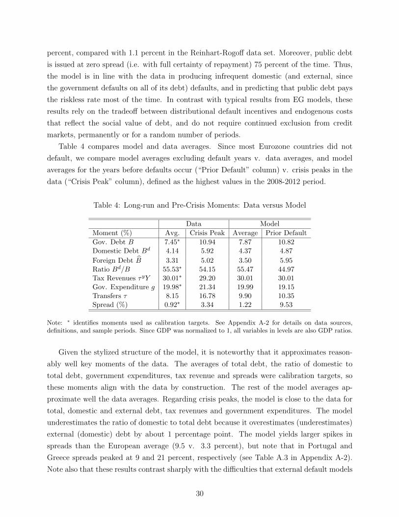
percent, compared with 1.1 percent in the Reinhart-Rogoff data set. Moreover, public debt

is issued at zero spread (i.e. with full certainty of repayment) 75 percent of the time. Thus,

the model is in line with the data in producing infrequent domestic (and external, since

the government defaults on all of its debt) defaults, and in predicting that public debt pays

the riskless rate most of the time. In contrast with typical results from EG models, these

results rely on the tradeoff between distributional default incentives and endogenous costs

that reflect the social value of debt, and do not require continued exclusion from credit

markets, permanently or for a random number of periods.

Table 4 compares model and data averages. Since most Eurozone countries did not

default, we compare model averages excluding default years v. data averages, and model

averages for the years before defaults occur (“Prior Default” column) v. crisis peaks in the

data (“Crisis Peak” column), defined as the highest values in the 2008-2012 period.

Table 4: Long-run and Pre-Crisis Moments: Data versus Model

Data Model

Moment (%) Avg. Crisis Peak Average Prior Default

Gov. Debt B 7.45∗ 10.94 7.87 10.82Domestic Debt Bd 4.14 5.92 4.37 4.87

Foreign Debt B 3.31 5.02 3.50 5.95Ratio Bd/B 55.53∗ 54.15 55.47 44.97Tax Revenues τyY 30.01∗ 29.20 30.01 30.01Gov. Expenditure g 19.98∗ 21.34 19.99 19.15Transfers τ 8.15 16.78 9.90 10.35Spread (%) 0.92∗ 3.34 1.22 9.53

Note: ∗ identifies moments used as calibration targets. See Appendix A-2 for details on data sources,definitions, and sample periods. Since GDP was normalized to 1, all variables in levels are also GDP ratios.

Given the stylized structure of the model, it is noteworthy that it approximates reason-

ably well key moments of the data. The averages of total debt, the ratio of domestic to

total debt, government expenditures, tax revenue and spreads were calibration targets, so

these moments align with the data by construction. The rest of the model averages ap-

proximate well the data averages. Regarding crisis peaks, the model is close to the data for

total, domestic and external debt, tax revenues and government expenditures. The model

underestimates the ratio of domestic to total debt because it overestimates (underestimates)

external (domestic) debt by about 1 percentage point. The model yields larger spikes in

spreads than the European average (9.5 v. 3.3 percent), but note that in Portugal and

Greece spreads peaked at 9 and 21 percent, respectively (see Table A.3 in Appendix A-2).

Note also that these results contrast sharply with the difficulties that external default models

30

often have in producing large spreads at reasonable debt ratios.

Table 5 compares standard deviations (relative to the standard deviation of income) and

correlations with disposable income and government expenditures. We use disposable income

because in the model it fluctuates with τ , while GDP is constant, and we report correlations

with government expenditures because g is the model’s exogenous aggregate shock. We

explain important effects of default risk in the model comparing results v. a version of the

model in which the government is committed to repay.

Table 5: Cyclical Moments: Data versus Model

Standard Dev. Correl(x, hhdi) Correl(x, g/GDP )

Model Model ModelBaseline w.o. Baseline w.o. Baseline w.o.

Variable x Data Model default Data Model default Data Model default

Disp. Inc. (hhdi) 1.05 1.75 1.64 1.00 1.00 1.00 -0.09 -0.58 -0.49Consumption 0.89 0.84 0.70 0.60 0.98 0.95 -0.31 -0.71 -0.60TB/GDP 0.68 0.60 0.57 -0.21 -0.86 -0.81 0.03 0.10 -0.18Spreads 0.35 1.79 - -0.33 -0.02 - -0.07 -0.26 -Gov. Debt / GDP 2.82 1.31 1.40 -0.26 -0.08 -0.65 0.40 -0.62 0.60Dom. Debt / GDP 2.15 0.24 0.39 -0.27 -0.31 -0.55 0.32 -0.30 0.43

Note: hhdi denotes household disposable income and TB denotes trade balance. In the model, hhdi =(1− τy)Y + τ and TB = Y −C − g. hhdi and C are logged and HP filtered with the smoothing parameterset to 6.25 (annual data). GDP ratios are also HP filtered with the same smoothing parameter. Standarddeviations of all variables except hhdi correspond to ratios to the standard deviations of hhdi. Since thesample for spreads is short (2002-2015) and for a period characterized by a sustained rise in spreads since2008, we generate comparable model data by isolating events spanning 10 years before spikes in spreads,defining spikes as observations in the 95 percentile. The standard deviation of spreads is demeaned to providea comparable variability ratio. See Appendix A-2 for details on data sources.

The model approximates closely the variability measures for consumption and net ex-

ports, and less so the ones for disposable income and total debt. It also matches the ranking

of variability of income, consumption and net exports. On the other hand, the model over-

estimates the variability of spreads and underestimates that of domestic debt. Regarding

income correlations, the model matches the data in producing a positive correlation with

consumption and negative correlations with net exports, spreads, total debt and domestic

debt. In terms of magnitudes, the correlations with spreads, total debt and domestic debt

are comparable with the data, but the consumption correlation is too high and the one with

net exports is too low. The model also matches closely the correlation between net exports

and spreads (0.03 in the data v. 0.10 in the model, not shown in the Table). This suggests

that foreign debt also has a weak correlation with spreads, since trade deficits are financed

with public debt sold abroad. Looking at correlations with government expenditures, the

31

model also does well at approximating those with consumption, net exports and spreads,

but it deviates sharply from the data in producing negative correlations of government ex-

penditures with total debt and domestic debt (-0.62 and -0.3), whereas the data show the

opposite (0.4 and 0.32), and it underestimates the correlation with income (-0.58 v. -0.09).

Comparing the baseline model results v. those for the model without default risk shows

that the negative correlations of total and domestic debt with government expenditures in

the former are due to default risk. Most moments do not differ much across the two cases,

but removing default risk shifts markedly the correlations between g and debt from negative

to positive (-0.62 to 0.6 for total debt and -0.3 to 0.43 for domestic debt), the correlations

between income and the two debt measures fall markedly (-0.08 to -0.65 for total debt and

-0.31 to -0.55 for domestic debt), and the correlation between g and income rises (from -

0.58 to -0.49). All these changes occur because without default risk the optimal public debt

choice smooths the effects of fluctuations in g on τ and income. Higher gt is less likely to

reduce disposable income because, following eq. (6), its negative effect on τt is hampered by

increasing debt so that (1/(1+r))Bt+1 rises. There is no debt Laffer curve because there is no

default risk. Hence, gt and Bt+1 are positively correlated and the correlation of income with

debt (government expenditures) is more (less) negative. With default risk, however, this

tax-smoothing objective can be more than offset by how the optimal debt choice responds to

the government’s reduced borrowing capacity and the Laffer curve of the resources generated

by new debt (qtBt+1). On average, increases in gt are now associated with reductions in Bt+1,

making these variables negatively correlated. This also sustains more states in which the

implied change in τ yields lower disposable income, making the correlation of income with

debt (government expenditures) less (more) negative. Notice spreads are also negatively

correlated with gt, indicating that the government chooses debt mindful of how it affects

bond prices and the resources new debt can yield.

The debt correlations in Table 5 may look closer to the data in the model without

default risk, but note that these correlations vary widely across countries, and for some

the correlations are more in line with the model with default risk. For instance, as Table

A.2 in the Appendix shows, the GDP-weighted average of the correlation of domestic debt

with government expenditures (0.32) is largely driven by the correlation for Germany (0.71),

which is by far the highest and the one with the largest GDP weight. In other countries this

correlation is zero or even negative (0.02 for Ireland, -0.19 for Spain, -0.03 for Netherlands).

It is also interesting that the positive correlation for Germany is in line with the model

with commitment and tax smoothing, whereas the negative one for Spain is closer to the

predictions of the model with default risk and reduced borrowing capacity.

We study next dynamics around default events. Figure 3 shows a set of 13-year default

32

event windows centered on the year of default at t = 0. These windows show averages for

defaults that start from the median debt of all default events at t = −6.24 Panel (i) shows

total, domestic and foreign debt holdings. Panel (ii) shows g and τ . Panel (iii) shows bond

spreads. Panel (iv) shows the social welfare gain of default denoted α.

Figure 3: Default Event Analysis

-7 -6 -5 -4 -3 -2 -1 0 1 2 3 4 5 6 7

period

0

0.02

0.04

0.06

0.08

0.1

0.12

0.14Panel (i): Debt and Default

1

-7 -6 -5 -4 -3 -2 -1 0 1 2 3 4 5 6 70.05

0.1

0.15

0.2

0.25

Gov

. Exp

. (g)

Panel (ii): Gov. Exp. and Gov Transfers

0.05

0.1

0.15

0.2

0.25

Gov

. Tra

nsfe

rs (

)

Panel (iii): Spreads

-7 -6 -5 -4 -3 -2 -1 0 1 2 3 4 5 6 7

period

0

2

4

6

8

10

Spre

ads

(%)

-7 -6 -5 -4 -3 -2 -1 0 1 2 3 4 5 6 7

period

-4

-3

-2

-1

0

1

We proceed as in Section 3 to compute α. First, we calculate individual percent compen-

sating variations in consumption α(b, y, B, g) that render agents identified by a (b, y) pair

indifferent between the payoffs V d=0(b, y, B, g) and V d=1(y, g) at the aggregate states (B, g):

α(b, y, B, g) = exp((V d=1(y, g)− V d=0(b, y, B, g))(1− β)

)− 1.

α(b, y, B, g) < 0 implies that agents with (b, y) prefer repayment. The social welfare gain of

24Appendix A-4 examines event windows similar to Figure 3 but starting from the lowest and highest debtsat t = −6 across all default events. Appendix A-5 examines two default events separated by a nondefaultphase that matches the mode duration of the nondefault state in the full simulation. These alternativeapproaches to study default dynamics yield similar qualitative findings as those reported here.

33

default is then computed as follows:

α(B, g) =

∫B×Y

α(b, y, B, g)dω(b, y).

Note that, since the functions involved are nonlinear, α is not the same as the compensating

variation that equates W d=0(B, g) and W d=1(g), but both measures are positive only when

the government defaults. Quantitatively, the differences between the two are negligible in

the calibrated model. We chose α(B, g) because it is easier to relate to individual welfare

gains. Keep in mind also that these social welfare measures aggregate individual payoffs

taken from the agents’ value functions, which reflect expected lifetime utility valuations, not

just comparisons of contemporaneous utility effects.

Panel (i) shows that total debt and the holdings of both foreign and domestic agents rise

in the first three periods, in tandem with lower g realizations (see Panel (ii)) and a slight

increase in spreads (see Panel (iii)). The three debt aggregates start near their long-run

averages at t = −6 . The increase in B is in line with the argument behind the negative

correlation between B and g discussed earlier: With debt already near its average, the

default risk mechanism inducing optimal debt issuance to rise when g falls dominates the

tax-smoothing mechanism. The higher debt finances higher τ , which allows the government

to do more progressive redistribution and provide more liquidity to credit-constrained agents.

Domestic agents increase their debt holdings only slightly because they were also near their

average holdings at t = −6, and these holdings fluctuate only about 1/4th as much as

income. Hence, the bulk of the early increase in B is absorbed by foreign creditors. Spreads

rise little because the distributional effects of the higher debt actually strengthen repayment

incentives (see Panel (iv)), with the social welfare gain of default falling from -2 percent at

t = −6 to close to -3 percent at t = −4. The probability of default still rises, because debt

is rising, but only slightly because default incentives weaken.

These early periods are followed by increasing realizations of g from t = −3 to the

default year t = 0. The same default risk mechanism now yields a reduction in debt at

t = −3 followed by constant debt the next two periods, together with rapidly increasing

spreads and default incentives. Since debt is very high, the slight increases in g lead the

government to borrow less in order to avoid a sharp rise in the default probability and

spreads (i.e. to avoid falling into the decreasing segment of the debt Laffer curve). The

fall in debt is again absorbed mainly by foreign creditors, as domestic debt holdings decline

slightly at t = −3 and then rise marginally in the following two periods. Spreads increase

first to about 2 percent and then spike to near 7 percent the year before the default occurs.25

25As spreads increase, they attract domestic agents with sufficiently high (b, y) to buy more debt, whichexplains the slight increase in domestic debt holdings.

34

Hence the model is consistent with the empirical observation of rapidly rising spreads during

debt crises. The social welfare gain of default also rises sharply, from close to -3 percent to

about -1.5 percent. With debt unchanged between t = −2 and t = −1, g rising slightly, and

distributional incentives now weakening sharply, the probability of default jumps causing

the jump in spreads.

At t = 0 the welfare gain of default jumps, reaching 1 percent, and since now default yields

a positive gain the government defaults. g rises slightly again but, at the high debt, this is

enough to cause the jump in α. The surge in spreads at t = −1 and the“sudden” default at

t = 0 occur with a debt ratio unchanged from the previous year. To an observer, the sudden

shifts in spreads and market access may suggest that the crisis resulted from multiplicity or

self-fulfilling expectations, but this is not the case. In addition, default occurs with relatively

low external debt, which is about a half of the total debt.

After the default, g rises again at t = 1, but now since debt starts at zero, the tax-

smoothing mechanism dominates, so that B rises with g. The social welfare gain of default

falls by 250 basis points from 1 to -1.5 percent, because the social value of debt is very high

at low debt. Domestic demand for debt rises gradually but sharply, since agents value highly

rebuilding precautionary savings but doing so implies sacrificing consumption. Hence, in the

early periods after the default foreign debt rises too, but after t = 2 the domestic debt ratio

grows bigger to about 4 percent and the foreign debt ratio declines to below 3 percent.The

total debt ratio stabilizes around 7 percent, and all through the six post-default years it is

sold at zero default risk. With debt this high, and g remaining close to 20 percent of GDP,

default incentives are strong but default is not optimal (α is barely below 0). We show

below in the analysis of the decision rules that in this situation (i.e., when domestic agents

desire to increase bond holdings but high g realizations weaken repayment incentives), the

government optimally chooses to place as much debt as it can at the risk-free price.

4.3 Equilibrium Recursive Functions

We analyze next the quantitative features of the equilibrium recursive functions, with the

aim of illustrating the model’s feedback mechanism and adding to the intuition behind the

time-series results. First we show that there are significant dispersion and asymmetries in

the individual welfare gains of default α(b, y, B, g) as we vary the aggregate states B, g.26

Figure 4 shows four graphs that plot the gains as a function of B for a range of realizations

of y. Panels (i) and (ii) are for b = 0 and b = 0.2, respectively, both with g = gL. Panels

(iii) and (iv) are also for b = 0 and b = 0.2, respectively, but now for g = gH .

26In the charts that follow, BH and BL denote 50 percent above and below the long-run average of debtBM = 0.079, ymax and ymin denote plus and minus 2 standard deviations of mean income µy = 0.78, andgH and gL denote plus and minus 2 standard deviations of mean government expenditures µg = 0.20.

35

Figure 4 yields three important results about the heterogeneity in default gains:

(1) Gains differ sharply across those who hold debt and those who do not. Panel (iii)

shows that the gains are mostly positive in all the domain of B for agents that do not hold

debt and draw any value of y when g is high, as these agents pay the same tax rate as debt

holders and do not suffer wealth losses from a default. The gains fall with y because agents

drawing higher income would have liked to use the bond market to save. For agents with

low y, however, the gains are negative when B is very low because these agents value highly

the liquidity and risk-sharing benefits of debt. Panels (i), (ii) and (iv) show a very different

pattern: default gains are almost always negative in the domain of B for agents with either

low or high b when g is low, and for agents with high b when g is high. The exception are

agents who do not hold debt and draw sufficiently high y when g is low and B is large (see

Panel (i)), because they value much less the benefits of public debt. In contrast, for agents

with b = 0.2 (Panels (ii) and (iv)), the gains are always negative and large in absolute value,

because a costly loss of wealth is the dominant factor for them.

Figure 4: Individual Gains from Default as a Function of B

0 0.05 0.1 0.15 0.2

Gov. Debt (B)

-15

-10

-5

0

0 0.05 0.1 0.15 0.2

Gov. Debt (B)

-15

-10

-5

0

0 0.05 0.1 0.15 0.2

Gov. Debt (B)

-5

0

5

10

0 0.05 0.1 0.15 0.2

Gov. Debt (B)

-5

0

5

10

(2) Gains are nonmonotonic in y. With b = 0 and g = gh (Panel (iii)), the gains are

higher for agents with lower y (except when B is very low for the reasons explained in (1)

above) because high-income agents who do not hold debt value more having access to the

36

bond market in order to start saving, and τ is smaller when g is high. In contrast, with

all the other combinations of b and g (Panels (i), (ii) and (iv)), the gains are smaller for

agents with lower y. Low-income agents with high b value more the loss of their assets due

to a default precisely when they would like to use their savings for self-insurance (recall that

defaults occur in periods of high g, which together with the debt freeze reduce τ sharply).

(3) Gains are increasing, convex functions of B for all y. This is most evident for agents

with b = 0 in Panel (iii), as they value increasingly more the progressive redistribution that

occurs when a larger B is defaulted on. For low B, default risk is not an issue, and hence

gains from default are linearly increasing, simply because of the cut in τ after a default. As B

rises, however, default risk starts to affect bond prices and demand for bonds, hampering the

ability of using bonds for self-insurance and liquidity-provision, and requiring increasingly

larger cuts in τ under repayment (as more resources are devoted to debt service). This

happens when the default probability at t+ 1 evaluated at t is positive, which is the case for

B > 0.05 and it is more evident for agents with low y who rely heavily on public transfers.

Figure 5 shows how α(b, y, B, g) responds to variations in g for different y values. This

figure is divided into four plots as the previous Figure, but now for different (b, B) pairs.

Panels (i) and (ii) are for b = 0 and b = 0.2 with a low supply of debt BL. Panels (iii) and

(iv) are for b = 0 and b = 0.2 with a high supply of debt BH .

Figure 5: Individual Gains from Default as a Function of g

0.17 0.18 0.19 0.2 0.21 0.22 0.23

Gov. Expenditures (g)

-14

-12

-10

-8

-6

-4

-2

0

2

0.17 0.18 0.19 0.2 0.21 0.22 0.23

Gov. Expenditures (g)

-14

-12

-10

-8

-6

-4

-2

0

2

0.17 0.18 0.19 0.2 0.21 0.22 0.23

Gov. Expenditures (g)

-12

-10

-8

-6

-4

-2

0

2

4

0.17 0.18 0.19 0.2 0.21 0.22 0.23

Gov. Expenditures (g)

-12

-10

-8

-6

-4

-2

0

2

4

37

Figure 5 shows similar dispersion and asymmetries in the individual default gains for

different g as those shown in Figure 4 for different B. In fact, Results (1)-(3) still hold, except

that Result (3) only holds for g < µg instead of for all g. This is because the exogenous

income cost making default costlier in “better” states of nature is only present when g is

below average. For g < µg, the gains are increasing and convex in g as a result of two forces:

First, the default cost falls as g rises. Second, default risk increases with g, and this lowers

bond prices and affects demand for bonds, resulting in lower transfers that reduce the value

of repayment. For g ≥ µg, the default gains become nearly independent of g, because the

adverse income effect of g via the exogenous default cost vanishes, and without it the effects

of higher g on repayment and default payoffs are of similar magnitudes. This occurs because

the direct effect of g reducing τ is the same for both, and under repayment default risk for

g > µg hampers the government’s use of debt for tax smoothing. The response of default

gains to increases in g is weaker for high-income agents (i.e. α curves are flatter for higher

y), because τ and the default cost represent a smaller share of their disposable income.

In addition, Figure 5 shows that default gains for the same y are uniformly higher for

agents who do not hold debt than for agents with b = 0.2 for all g realizations, just like it

was the case for all B in Figure 4. This is because τ is lower and default risk higher under

repayment for higher g. Looking now at income variations, the gains are lower (higher) at

lower y for agents with (without) bonds for g ≥ µg. For g < µg, however, the gains are

for the most part lower for agents with lower y regardless of bond holdings, because in this

range of g disposable individual income is reduced by both the lower y and the default cost,

which is uniform across agents.

The heterogeneity in default gains as g varies adds another key result:

(4) Government default incentives are weaker (stronger) when g is below (above) µg. All

agents favor repayment and by more at lower y for g slightly below average, but for above-

average g the gains differ in sign and in how they vary across agents with different income

and bond holdings. Non-bond holders prefer default and those with low income prefer it the

most, while bond holders (b = 0.2) prefer repayment and those with low income prefer it

the most. This result is behind the result from the event analysis showing generally lower α

and higher Bt+1 in periods with gt < µg, although the relationship is not monotonic because

both B and g are changing every period.

Next we study how the heterogeneity in individual default gains affects the social welfare

gains of default and the default decision rule. Figure 6 shows plots of α as a function of B

(Panel (i)) and g (Panel (ii)). These plots inherit the properties of the individual default

gains: The social gain of default is increasing and convex in B for all g and in g for all B if

g ≤ µg, while for g > µg the social gain of default is nearly independent of g (with the kink

38

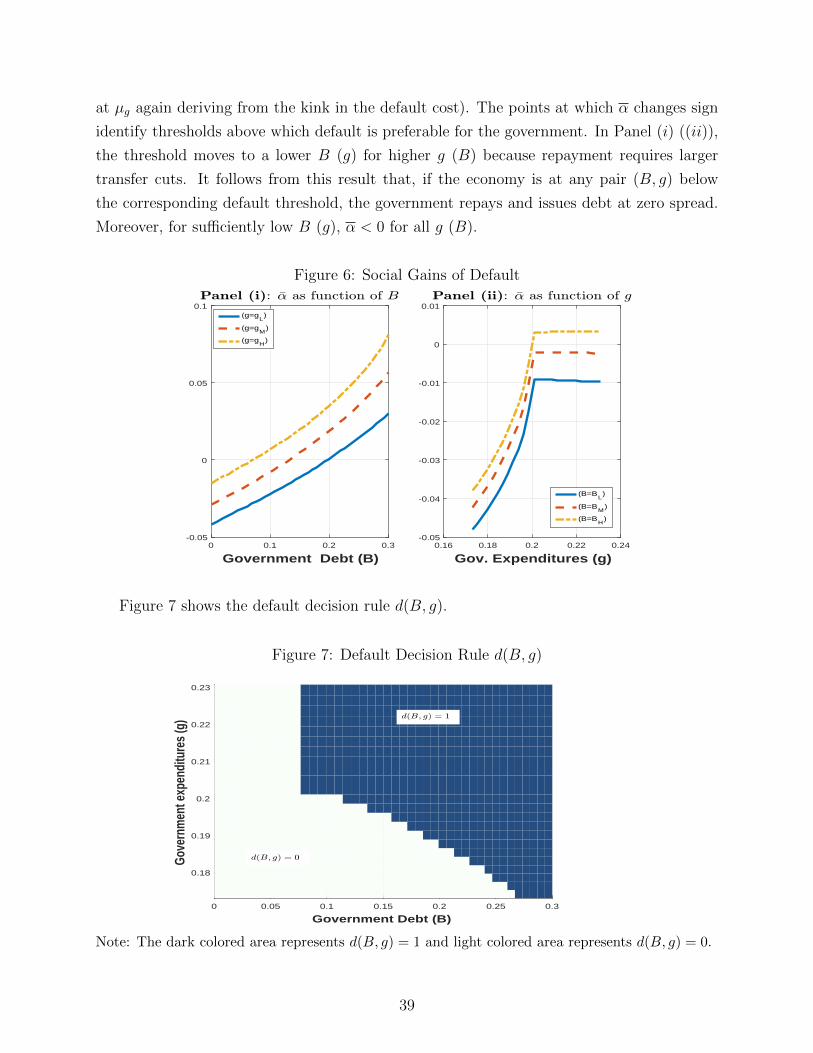
at µg again deriving from the kink in the default cost). The points at which α changes sign

identify thresholds above which default is preferable for the government. In Panel (i) ((ii)),

the threshold moves to a lower B (g) for higher g (B) because repayment requires larger

transfer cuts. It follows from this result that, if the economy is at any pair (B, g) below

the corresponding default threshold, the government repays and issues debt at zero spread.

Moreover, for sufficiently low B (g), α < 0 for all g (B).

Figure 6: Social Gains of Default

0 0.1 0.2 0.3

Government Debt (B)

-0.05

0

0.05

0.1(g=g

L)

(g=gM

)

(g=gH

)

0.16 0.18 0.2 0.22 0.24

Gov. Expenditures (g)

-0.05

-0.04

-0.03

-0.02

-0.01

0

0.01

(B=BL)

(B=BM

)

(B=BH

)

Figure 7 shows the default decision rule d(B, g).

Figure 7: Default Decision Rule d(B, g)

0 0.05 0.1 0.15 0.2 0.25 0.3

Government Debt (B)

0.18

0.19

0.2

0.21

0.22

0.23

Gove

rnm

ent e

xpen

ditu

res

(g)

Note: The dark colored area represents d(B, g) = 1 and light colored area represents d(B, g) = 0.

39

The default and repayment sets are identified in dark and white colors, respectively. Their

features are implied by the shifts in the thresholds of the social welfare gains from default

noted above. Since Figure 6 shows that α(B, g) < 0 for all g when B < 0.07, d(B, g) = 0 in

that same region. If the optimal debt choice falls in this region, that debt is issued with full

certainty of repayment. For 0.07 ≤ B ≤ 0.25, there is a high enough threshold value of g

such that above it the government defaults and below it repays, and the threshold is lower

at higher B. For debt to be issued exposed to default risk at equilibrium, the optimal debt

choice must fall in this region along the equilibrium path. For B > 0.27, the government

defaults for all g, and new debt cannot be issued because default would occur with certainty.

Note that the default and repayment sets are not symmetric because of the asymmetry in

the default cost, which lowers disposable income only if default occurs with g < µg.

A limitation of examining the social and individual default gains is that one can either

look at α, which hides the dispersion of the individual gains, or look at the individual αs,

which are uninformative about the default choice since it hinges on social valuations. To

illustrate the interaction between the two, and their effect on the default decision, Figure 8

shows the social distributions of default gains for particular (B, g) pairs.

Figure 8: Social Distributions of Individual Default Gains for Different B and g

-0.05 0 0.05

Ind. utility gains from default ( )

0

10

20

30

40

50

60

70

80

90

100

Frac

Hou

seho

lds

(%)

-0.05 0 0.05

Ind. utility gains from default ( )

0

10

20

30

40

50

60

70

80

90

100

Frac

Hou

seho

lds

(%)

These are distributions of the αs induced by the welfare weights ω(b, y) for four pairs of

(B, g) formed by combining BL, BH and gL, gH .27 The average of each of these distributions

27These plots show cumulative distribution functions (CDF) of α(b, y, B, g) for given (B, g) across all (b, y)pairs. Given a (B, g) pair, each (b, y) maps into a value of α(b, y, B, g) and a welfare weight ω(b, y). TheCDFs are constructed by sorting the α(b, y, B, g) from low to high and integrating over (b, y) using ω(b, y).

40

corresponds to a point in the plots of the α curves shown in Figure 6 for the corresponding

(B, g) pair. These distributions are not the same as ω(b, y), because the nonlinear, non-

monotonic responses of the individual αs to changes in B and g discussed earlier imply that

the αs move in different directions across (b, y) pairs when (B, g) changes.28

Figure 8 is important because it shows the relevance of agent heterogeneity in the

sovereign’s aggregation of default gains (even tough the welfare weights ω(b, y) are fixed),

and how it varies with B and g, shifting to the right as B (g) rises for given g (B). Panel (i)

shows that, since for either BL or BH default is never chosen for g = gL < 0.177 (see Figure

7), the social distributions of default gains have most of their mass in the negative quadrant,

which represents agents who prefer repayment. In contrast, the distribution in Panel (ii)

for the case with g = gH and B = BH has enough mass in the positive quadrant to yield

a positive mean, which makes default socially optimal. Even in this case, however, about

32 percent of agents are better off under repayment in the planner’s valuation (this is the

cumulative social valuation of agents with negative αs for (BH , gH)). These distributions

also reflect the asymmetric effects of above- v. below-average g shocks on the individual αs:

The distributions for gL in Panel (i) are skewed to the left compared with those for gH in

Panel (ii), even tough the g shocks are symmetric, the two panels use the same two values

of B, and the welfare weights are the same.

The welfare weights used to construct Figure 8 differ from the distribution of debt and

income across agents, which implies that the social welfare function is not utilitarian. In-

stead of assigning equal weight to all agents, and thus aggregate individual utilities with

Γt(b, y), the weights determined by ω(b, y) display the creditor bias implied by ω. Com-

paring these weights with the average distribution of debt and income in the time-series

simulation (Γ(b, y)), we find that both mass 90 percent of agents with debt holdings below

0.15 and close to 100 percent below 0.5.29 They also mass similar fractions of agents with

debt holdings below 0.1, at 88 and 78 percent for ω(b, y) and Γ(b, y), respectively. The two

differ significantly, however, in the weight assigned to agents at or near zero debt holdings

(i.e. below 0.01), 81.0 percent for Γ(b, y) v. 15 percent with ω(b, y). Hence, while agents

with mid to large debt holdings are weighted similarly by ω(b, y) and Γ(b, y), calibrating the

model to match the observed mean spreads (at the observed mean ratios of total debt to

GDP and domestic debt to total debt) requires a value of ω that reduces sharply the weight

the sovereign assigns to non-debt-holders relative to their share in the distribution of debt.

Without this, default incentives are too strong and the sustainable debt ratios too small.

28This is also evident in the intensity plots of α(b, y, B, g) in the (b, y) space included in Appendix A-6,which display regions with similar colors (i.e., similar αs) for different (b, y) pairs.

29We report the average because Γt(b, y) is time- and state-contingent. Default episodes are excluded fromthis calculation. See Appendix A-7 for a detailed comparison of ω(b, y) and Γ(b, y).

41

Despite the much larger weight on non-debt-holders in ω(b, y) relative to Γ(b, y), the

weights given by ω(b, y) are actually a much better approximation to the actual distribution

of asset holdings in the Eurozone than Γ(b, y).30 The ECB’s 2016 Household Finance and

Consumption Survey reports that the shares of net wealth held by the top 10 and 5 percent

of agents are 51.2 and 37.8 percent, respectively.31 In the model, the corresponding weights

implied by ω(.) are 33.1 and 20.3 percent, respectively, while those implied by Γ(.) are 86.8

percent and 62.7 percent, respectively. The ratios of the median debt holdings to the top 10

percent of the distribution of debt are 20.8 percent in the data v. 29.2 and 0 percent in ω(.)

and Γ(.), respectively. Hence, Γ(.) overestimates (underestimates) significantly the fraction

of wealth owned by agents at the top (bottom) of the distribution relative to both the data

and ω(.). This also suggests that modeling a social welfare function with creditor bias is a

reasonable benchmark.

Consider next the equilibrium pricing function of debt and the debt Laffer curve. Panel

(i) of Figure 9 shows the pricing function as a function of new debt issuance B′ for four

values of g, and Panel (ii) shows the corresponding Laffer curves.

Figure 9: Pricing Function q(B′, g) and Debt Laffer Curve

0 0.05 0.1 0.15 0.2 0.25 0.3

0

0.1

0.2

0.3

0.4

0.5

0.6

0.7

0.8

0.9

1

0 0.05 0.1 0.15 0.2 0.25 0.3

0

0.02

0.04

0.06

0.08

0.1

0.12

0.14

0.16

0.18

0.2

Note: Circles on the curves with g ∈ gL, gM , gH mark the optimal debt choice for the corresponding valueof g and with B = BM . The circles for curves with g = g9 (the ninth element in the Markov vector of g)

denote the optimal debt choice when B = 0.106. This (B, g) pair is the one observed at t = −1 in Figure 3.

Figure 9 includes results for gL, µg, and gH , and also for g = g9 = 0.193 (the ninth

30The result that Γ(.) does not match well the actual wealth distribution, particularly its concentration,is a well-known feature of standard heterogeneous-agents models. Extensions with preference heterogeneityand a life-cycle structure perform better (see Heathcote et. al. [37] and Krueger et al [39]).

31See Table 4.1 in www.ecb.europa.eu/pub/pdf/scpsps/ecbsp18.en.pdf?d2911394a25c444cd8d3db4b77e8891a.

42

element in the Markov vector of g), which is the realization observed at t = −1, just before

the default in Panel (ii) of Figure 3. We marked with circles the optimal choice of B′, which

are the values implied by the equilibrium decision rule B′(B, g). For g = gL, gM , gH we

use B = BM and for g = g9 we use B = 0.106, which is the value observed at t = −1 in

Figure 3.

Since bond prices satisfy the same no-arbitrage condition of foreign investors as in EG

models, the pricing functions have a similar shape. If B′ is low enough for default in the next

period to have zero probability, q equals the risk-free price 1/(1+ r). Conversely, if B′ is high

enough for default to be expected with probability 1, the bond market collapses and q = 0.

In between these two regions, q falls rapidly as B′ rises, because the probability of default

rises at an increasing rate as more debt is issued. For debt that carries default risk, prices

are lower at higher g, because the probability of default is also higher at higher g for given

B′.32 Despite these similarities with EG models, the default probability driving q here is

determined in a very different way, with the government taking into account the distribution

of gains from default across all domestic agents, including domestic bond holders.

The debt Laffer curves in Panel (ii) show how the resources obtained by issuing debt,

q(B′, g)B′, vary with B′. These Laffer curves first increase linearly when debt is issued at the

risk-free price, because q is constant, then they turn increasing but approximately concave

as debt rises enough to produce moderate increases in default risk, and then turn decreasing

and drop sharply, in line with the steep pricing functions of Panel (i). Note also that the

Laffer curves shift down and to the left as g rises (for given B), indicating that the ability

to use debt for progressive redistribution weakens considerably as g increases.

The optimal debt choices circled in Panels (i) and (ii) reflect the tradeoffs between

distributional incentives and social value of debt faced by the government. There are three

regions where the debt choice can be located: First, unconstrained debt at zero spread. For

low enough g and/or B, debt is sold at the risk-free price and the optimal debt is located

along the upward-sloping segment of the Laffer curve (e.g. the case for g = gL). Second,

constrained debt at zero spread. These are states with (B, g) such that new debt is still sold

at the risk-free price but the optimal debt is set at the maximum of the Laffer curve, so that

it yields the most resources new debt can yield (e.g. the cases for gM and gH). Less debt is

suboptimal, because it generates fewer resources than desired and the Laffer curve is linearly

increasing. More debt is suboptimal, because default risk rises rapidly, making bond prices

drop sharply and thus yielding much fewer resources. Hence, in this region, the government’s

32Notice this is a statement about how the realization gt affects the probability of a default at t+1, whereaswhat we showed earlier is that, for sufficiently large Bt+1, the government optimally chooses to default att+ 1 if gt+1 exceeds a threshold value. However, pt(Bt+1, gt) rises with gt because g shocks approximate anAR(1) process with 0.86 autocorrelation.

43

option to default does not generate a positive spread but limits significantly its borrowing

ability. Third, constrained debt with positive spread (i.e. defaultable debt). Debt is sold

with a positive spread and the optimal debt choice may be at the maximum of the Laffer

curve or less. The case for g9 yields optimal debt below the maximum of the Laffer curve,

but for slightly higher g the maximum is optimal. In this region, the sovereign desires more

resources than what debt sold at the risk-free price can generate, but not always as many

as the most it can generate with a positive spread. The option to default again restricts the

government’s ability to sustain debt. Along the equilibrium path, debt is in the third region

less frequently than in the second, so that debt has no risk premium most of the time but

its amount is still constrained by the government’s inability to commit.

The case with g = g9 is also interesting because it is the outcome observed in the model’s

equilibrium path in the period before the default events studied in Figure 3. The fact that

optimal debt sold at t = −1 is lower than the maximum value of the Laffer curve indicates

that the progressive redistribution attained by selling less debt at a higher price, but smaller

than the risk-free price, is socially preferable to selling more debt at a lower price even if it

yields more resources, including in both counts the social benefits of debt. The government

defaults at t = 0 because the regressive redistribution induced by repaying plus the value of

the social benefits of debt, is less desirable than the progressive redistribution net of the loss

of the social benefits of debt and the exogenous default cost, attained by defaulting.

In terms of the dependency of the debt choice on B, we use the quantitative results to

show in Appendix A-6 that, depending on g, the debt choice is either nearly independent of

B or increasing in B. It is nearly independent of B for g ≥ µg, because the optimal debt

is the maximum value of the Laffer curve regardless of the value of B, and this maximum

does not vary much with B because, as shown earlier, social and individual welfare gains

of default are nearly independent of B when g ≥ µg due to the asymmetry neutralizing the

exogenous default cost (e.g. the optimal debt is 0.107 for gM and 0.071 for gH for most of the

domain of B). In this interval of g, debt is sold at the risk-free price but as explained earlier

it is still constrained by the government’s default option. For g < µg, the optimal debt rises

with B and is always below the maximum of the Laffer curve. Hence, it is at these levels of

g that the government can choose debt lower than the maximum value of the Laffer curve,

and in some of these states it is optimal to issue debt that carries a default risk premium.

4.4 Sensitivity Analysis & Extensions

To close this Section, we conduct a sensitivity analysis of the quantitative implications of

altering the values of key parameters and adding important features to the model.

(a) Welfare Weights

We examine the implications of altering the welfare weights by making two kinds of

44

comparisons. First, we adopt the following more general formulation of ω(b, y):

ω(b, y) =∑yi≤y

π∗(yi)(

1− e−(b+z)ω

). (37)

ω still measures creditor bias, but now z controls the weight assigned to agents who do not

hold debt (i.e. those hitting the borrowing constraint). These are the agents receiving the

liquidity benefit of debt, and the largest redistribution of resources when new debt is issued

under repayment or when outstanding debt is wiped out under default. Second, we study

a case akin to a utilitarian sovereign by replacing ω(b, y) with the long-run average of the

distribution of (b, y) across agents for the model without default risk, Γrf

(b, y).33

Table 6 compares the results for the Baseline calibration v. three scenarios with different

values of ω and z (cases (A)-(C)), and the case with ω(b, y) = Γrf

(b, y) (case (D)). We report

long-run averages and averages before default events, and three additional sets of statistics

that help explain the results. First, the cumulative welfare weights for agents with bond

holdings up to a given amount across all income levels, defined as Ω(b) =∑

y∈Y ω(b, y). We

consider agents with b up to 0, 0.0004, 0.045 and 0.30, because in the calibrated ω(b, y)

function they yield cumulative weights of 0, 1, 50 and 99 percent respectively. Second, we

use equation (28) to report the threshold bond holdings b(µy, BD, gD) of an agent who draws

income µy and is indifferent between repayment and default when B and g are at their

averages conditional on the government choosing to default (BD, gD). Agents with b ≥ b

prefer repayment. Third, we report the fraction of agents that favor repayment according

to the CDF of the mean distribution of bond and income of each model solution (the mean

distribution is denoted Γ(b, y), and the CDF is γ(b, y)), and the comparable fraction as

valued by the government using ω(b, y).

Comparing the Baseline column with column (A) shows the effects of increasing z from

0 to 0.025. This increases the welfare weight of agents without debt from 0 to 32.06 percent.

The cumulative weights of agents with b up to either 0.0004 or 0.045 also rise, to 32.29 and

67.09 percent, respectively v. 1 and 50 percent, respectively in the Baseline. b drops from

0.095 to 0.068, and the fraction of agents that the government sees as gaining from repayment

drops from 22.4 to 21.9 percent, while the actual fraction of agents that favor repayment

rises from 4.5 to 5.2 percent. These changes indicate stronger incentives to default, in line

with the analysis in the first exercise of Section 3: By assigning positive weight to agents

with b = 0 (and in general higher weight to agents with lower b), the fraction of agents that

the government assesses as gaining from a default is closer to the corresponding fraction in

the economy’s wealth distribution, which reduces incentives to repay. The stronger default

33Results using the average distribution of the model with default are quantitatively similar.

45

incentives result in a lower mean debt ratio and higher mean spreads and default frequency.

The mean domestic and external debt ratios also drop, but the ratio of domestic to external

rises sharply, from 1.25 to 2.81. Qualitatively similar changes are observed in the averages

of these statistics prior to defaults.

Table 6: Sensitivity Analysis: Social Welfare Weights

Baseline (A) (B) ( C ) (D)ω = 0.065 ω = 0.065 ω = 0.055 ω = 0.055 ω(b, y)

Moment (%) z = 0 z = 0.025 z = 0 z = 0.025 = Γrf (b, y)Long Run Avg.Gov. Debt B 7.87 5.71 6.61 4.93 3.76Dom. Debt Bd 4.37 4.21 4.27 4.14 3.23

Foreign Debt B 3.50 1.50 2.35 0.79 0.53Default Frequency 1.21 2.26 2.10 3.52 4.39Spreads 1.22 2.32 2.15 3.65 4.592Transf τ 9.90 9.93 9.92 9.95 10.01Frac. Hh’s b = 0 65.58 67.42 67.69 67.33 69.64α(B, g) -0.814 -0.781 -0.862 -0.766 -0.768Avg. Prior DefaultGov. Debt B 10.82 7.99 9.26 6.97 5.43Dom. Debt Bd 4.87 4.79 4.95 4.76 4.28

Foreign Debt B 5.95 3.20 4.32 2.21 1.15Spreads 9.53 12.67 12.30 19.78 16.16

Def. Th. b(µy) 0.095 0.068 0.081 0.060 0.049

%. Favor Repay (1-ω(b(µy), µy)) 22.44 21.92 21.59 20.48 4.91

% Favor Repay (1-γ(b(µy), µy)) 4.48 5.19 4.97 5.51 5.53Cumulative Welfare WeightsΩ(b = 0) 0.00 32.06 0.00 36.59 65.64Ω(b = 0.0004) 1.00 32.29 0.51 36.84 65.65Ω(b = 0.0447) 50.00 67.09 57.48 73.01 85.83Ω(b = 0.3025) 99.00 99.41 99.63 99.77 93.82

Note: All moments reported correspond to averages excluding default periods, except those labeled “Avg.Prior Default” which correspond to the average of observations prior to a default event. The model issimulated 160 times for 10,000 periods, truncating the initial 2,000 periods.

Reducing ω to 0.055 (a 15 percent cut), while keeping z = 0, also strengthens default

incentives (compare columns (B) v. Baseline). Agents without bond holdings have the same

zero welfare weight as in the Baseline, but the weight of agents with relatively small b rises.

The cumulative welfare weights of agents with b up to 0.0004 and 0.045 increase, but less

so than in the scenario with z > 0. Hence, we get the same results qualitatively, but the

46

effects are weaker quantitatively. Introducing both higher z and lower ω (Column (C)) has

again similar qualitative effects relative to the Baseline, but quantitatively the effects are

now stronger. Agents without bond holdings have a cumulative welfare weight of nearly 36.6

percent, and the weight of agents with b up to 0.045 increases from 50 to 73 percent.

Using Γrf

(b, y) to define welfare weights also has qualitatively similar effects, but quan-

titatively the effects are the strongest of all the scenarios. This is because Γrf

(b, y) assigns

more weight to agents with low b than any of the other cases. In fact, the fraction of agents

the government sees as in favor of repayment falls sharply to 4.9 percent, and is now about

the same as what the mean distribution of bonds and income yields. As before, this results

in higher spreads and lower debt. The increase in default risk also reduces the domestic

demand for government bonds but by much less than the decline in total debt, resulting in

a much higher ratio of domestic to external debt.

Summing up, altering the welfare weights does change the quantitative results, but in

all cases the model sustains sizable debt ratios at nontrivial spreads. This is the case for

either arbitrary ω functions that assign large welfare weights to agents with little or no

debt holdings, or if the welfare weights are set to match the long-run average distribution of

bonds and income across agents. The drawback under the alternative formulations is that

the predicted spreads and default frequencies are much higher than what is observed in the

data. Matching these requires stronger creditor bias on the part of the sovereign.

(b) Preference Parameters and Income Process

Table 7 shows results from solving the model for higher and lower β, σ, and σu than in

the Baseline. These parameters are key determinants of precautionary savings, and hence

are important for driving the model’s results. Note that, since bond prices are determined

by the no-arbitrage condition of foreign investors, bond prices are affected only indirectly

through the default probability determined by the government’s debt and default decisions.

In particular, changes in σ do not affect bond prices directly via domestic marginal rates of

substitution in consumption, although this is still a determinant of domestic bond demand.

The effects on Bd are standard from the incomplete-markets theory of savings: Increasing

(reducing) incentives for self-insurance by rising (lowering) β, σ, or σu, increases (reduces)

the long-run and before-default averages of domestic bond holdings. The effects on foreign

debt are in the opposite direction, so the ratio of domestic to external debt rises (falls)

as precautionary savings strengthens (weakens). With higher β, σ, or σu, domestic bond

demand rises so much that almost all the debt ends up being domestic (with σ = 1.25, the

economy even becomes a net external creditor). The changes in total debt, on the other

hand, are nonmonotonic with respect to changes in β and σu: Debt is higher in the scenarios

in which these parameters are higher or lower than their corresponding values in the Baseline.

47

Table 7: Sensitivity Analysis: Preference Parameters and Income Process

β σ σuMoment (%) Baseline 0.853 0.888 0.75 1.25 0† 0.28 0.34

Long Run Avg.

Gov. Debt B 7.87 7.90 8.03 7.79 7.90 2.82 7.86 7.88Dom. Debt Bd 4.37 2.45 7.53 1.05 10.07 0.00 2.85 5.92

Foreign Debt B 3.50 5.46 0.50 6.74 -2.16 2.82 5.01 1.96Def. Freq. 1.21 1.23 1.19 1.26 1.19 8.92 1.21 1.18Spreads 1.22 1.24 1.21 1.278 1.202 9.793 1.224 1.199Transf τ 9.896 9.895 9.897 9.896 9.896 10.35 9.896 9.896Frac. Hh’s b = 0 65.58 82.99 60.07 88.75 55.67 99.99 81.30 63.28α(B, g) -0.814 -0.946 -0.698 -0.771 -0.877 -0.666 -0.803 -0.827

Avg. Prior Default

Gov. Debt B 10.82 10.84 10.74 10.24 10.78 3.73 10.80 10.82Dom. Debt Bd 4.87 2.78 8.52 1.17 10.60 0.00 3.22 6.74

Foreign Debt B 5.95 8.06 2.22 9.08 0.17 3.73 7.57 4.08Spreads 9.530 9.495 9.631 9.299 9.563 14.76 9.562 9.530

Note: Baseline model parameters are β = 0.871, σ = 1 and σu = 0.31. † This case has no idiosyncraticuncertainty and income for all agents is set to mean income µy. Also, the welfare function is adjusted tocoincide with the observed distribution where all agents hold no bonds. All moments reported are averagesexcluding default, except those labeled “Avg. Prior Default” which are averages of observations prior to adefault event. The model is simulated 160 times for 10,000 periods and we drop the initial 2,000 periods.

Higher σ or σu reduce default incentives and yield lower spreads and default frequencies,

because the social gain of default falls. The benefit of defaulting as a mechanism to substitute

for redistribution through risk-sharing with debt decreases, while on the other hand the social

value of debt for the provision of liquidity and the accumulation of precautionary savings

rises. In the scenario with higher β, in addition to the effects via domestic bond demand,

higher discounting makes default costlier, because the government values less the benefit

of providing assets for self-insurance for future consumption smoothing. While, as in EG

models, the government’s incentive to borrow also decreases at a higher β, the effect of the

higher endogenous default costs dominates and results in higher debt than in the baseline

rendering the debt ratio locally non-monotonic in β.

The case with σu = 0 is of particular interest, because removing individual income shocks

renders the model equivalent to an EG model with a representative domestic agent.34 The

volatility of g and the default risk do not generate enough variation in aggregate disposable

income to yield a positive net foreign asset (NFA) position (i.e. assets held abroad for self-

insurance), so the government issues debt abroad and the NFA position is negative. The

34This experiment can be solved with the same algorithm as the others by setting ω ≈ 0, so that thesovereign does not assign weight to “artificially” heterogeneous agents by weighting the agents’ value functionsin all the nodes of the grid of bonds.

48

results are in line with standard EG models: the average debt falls sharply and the default

frequency is much higher than in the Baseline.

In summary, in these experiments we find again that the model sustains sizable debt

exposed to default risk with infrequent defaults. Domestic debt and the ratio of domestic

to foreign debt are more sensitive to the parameter variations we considered than the other

model statistics. We also showed that agent heterogeneity is of major relevance for the

results, because a comparable EG representative-agent version of the model sustains much

less debt and overestimates spreads and the default frequency significantly.

(c) Income Tax Rate and Default Cost

Table 8 reports the effects of changes in the income tax rate (τ y) and the exogenous

default cost function (φ(g)). For the latter, we use the following generalization of φ(g):

φ(g) = φ1 max0, (g − g)ψ.

Here, g denotes the threshold realization of g at which the cost vanishes, and ψ controls the

curvature of the cost function. In the baseline calibration, g = µg, ψ = 1/2, and φ1 was

calibrated to target the Eurozone’s mean spread.

Table 8: Sensitivity Analysis: Income Taxes and Default Cost

τy φ1 ψ g

Moment (%) Baseline 0.29 0.48 0.59 0.99 0.40 0.60 0.188 0.209

Long Run Avg.

Gov. Debt B 7.87 7.85 7.87 7.36 8.23 8.26 7.19 6.80 13.52Dom. Debt Bd 4.37 7.41 2.33 4.22 5.48 4.41 4.24 4.22 4.44

Foreign Debt B 3.50 0.45 5.54 3.14 2.75 3.85 2.96 2.58 9.09Def. Freq. 1.21 1.21 1.18 0.42 4.10 1.30 0.31 0.06 2.64Spreads 1.220 1.223 1.189 0.42 4.28 1.32 0.31 0.06 2.71Transf τ 9.896 2.40 17.41 9.898 10.91 9.89 9.90 9.90 9.74Frac. Hh’s b = 0 65.58 59.94 83.08 66.85 73.63 65.35 66.34 65.68 66.79α(B, g) -0.814 -0.897 -0.766 -0.636 -3.880 -1.046 -0.541 -0.213 -1.963

Avg. Prior Default

Gov. Debt B 10.82 10.78 10.82 9.40 9.97 12.02 9.03 11.03 18.62Dom. Debt Bd 4.87 8.31 2.66 4.56 5.85 5.08 4.54 5.37 4.46

Foreign Debt B 5.95 2.47 8.16 4.85 4.12 6.94 4.49 5.65 14.15Spreads 9.530 9.560 9.524 4.207 10.33 10.42 2.98 8.46 11.34

Note: Baseline parameters are τy = 0.386, φ1 = 0.793, ψ = 1/2 and g = 0.199. All moments reported areaverages excluding default, except those labeled “Avg. Prior Default” which are averages prior to a defaultevent. The model is simulated 160 times for 10,000 periods, dropping the initial 2,000.

Comparing Tables 7 and 8, shows that higher (lower) τ y has similar qualitative effects as

49

lower (higher) σu. This is in part because both parameters affect the variance of idiosyncratic

disposable income, which is equal to (1 − τ y)2σ2y. In addition, as explained in Section 2,

a higher τy improves the implicit cross-sectional sharing of idiosyncratic risk provided by

government transfers. Hence, these results can be viewed as showing the implications of

allowing the government to use means other than debt and default to redistribute resources.

The Baseline predictions with a τy = 0.35 are not altered much by changing the tax to 0.20

or 0.45, except for the allocation of debt holdings across foreign and domestic agents, with

the share of the former being much higher at higher tax rates.

Regarding changes in the default cost function, changes that increase the cost (higher

φ1, lower ψ, or higher g) weaken incentives to default and allow the government to sustain

more debt on average. Everything else the same, weaker default incentives should reduce

the probability of default and yield lower spreads, but since the weaker incentives also make

it optimal for the government to issue more debt (note that the mean social welfare gain

of default falls with the higher default costs), the equilibrium default probabilities for the

higher debt are higher, resulting in higher spreads. Higher spreads induce an increase in

domestic demand for debt. Average debt ratios in the years before defaults occur are also

higher with the higher default costs (except in the case of φ1 = 0.99), and in the three cases

the average spreads before defaults are higher.

These results are important because they show the extent to which the model’s predictions

hinge on the exogenous default cost. The value of φ1 is relevant mainly for the spreads, while

the other model moments are less affected. Still, even with a value reduced to three-quarters

the size of that in the baseline calibration, the long-run mean spread is about 42 basis points

and the average spread before defaults is 421 basis points. The threshold g was shown earlier

to be important for explaining the dispersion of individual default gains, the government’s

default incentives, and the association of periods of increasing debt with low g realizations.

Here, we showed in addition that lowering g, so that the exogenous default cost is active for

a narrower range of realizations of g, has a small effect on total debt and its domestic and

external components. On the other hand, the average social gains of default are significantly

higher and spreads are sharply lower. The effects of increasing ψ are similar, since higher ψ

lowers the marginal cost of a given reduction of g below the threshold, suggesting that lower

g could be traded for lower ψ without altering the results significantly.

In all the results shown in Table 8, the model again sustains sizable ratios of total and

domestic debt exposed to default risk. Spreads are also non-trivial and default remains an

infrequent event preceded by sudden, sharp increases in debt and spreads. The model’s

ability to produce sizable spreads, however, does depend on the exogenous cost. In light of

these findings, we examine the model’s predictions if the exogenous cost is removed (φ1 = 0).

50

This case still yields sizable debt, with long-run mean debt ratios of total and domestic debt

of 5.6 and 4.3 percent respectively, but with a zero mean spread. Debt is optimally chosen to

sell at the risk-free price, as incentives to default weaken considerably, resulting in a social

gain of default that is still negative but higher than in the Baseline and close to zero, at -

0.07 percent. Contrary to the perfect-foresight analysis of Section 3, default does not become

generally optimal without exogenous costs, because the endogenous costs due to the social

value of debt are large. Spreads are zero, however, because the bond pricing function is too

steep at debt levels that could be offered with positive spreads, which leads the government

to prefer issuing risk-free debt. Hence, as noted earlier, the debt is sold at the risk-free price

but the government’s borrowing capacity is hampered by its inability to commit to repay.

(d) Partial Default

The last experiment examines the implications of altering the assumption that default

requires reneging on all of the debt (i.e. a default rate of ϕ = 1). Table 9 presents results

for exogenous default rates set to ϕ =∈ 0.90, 0.80, 0.50 (cases (A), (B), and (C)). The

government repays the fraction (1 − ϕ) of its debt during the exclusion period. Case (D)

shows results for a setup in which the government chooses ϕ ∈ [0, 1] optimally. To solve it, we

first solve an auxiliary problem to compute how much each agent values an outcome with a

given ϕ (similar to the problem we solve to find the optimal debt issuance). We then integrate

the resulting individual indirect utility functions to obtain the associated social welfare value

for each ϕ and let the government choose the one that maximizes welfare. These experiments

shed light on the potential effects of renegotiation that yields debt haircuts at the rate ϕ,

the possibility of partial commitment to repay, and the implications of considering partial

default mechanisms such as the erosion of nominal debt by inflation, the introduction of

wealth or financial taxes, and adjustments in eligibility criteria for entitlement programs

(e.g. retirement ages for pensions, needs-based rules for health programs).

The model with endogenous default rate (case (D)) yields the result that along the

equilibrium path, if the government chooses to default it always chooses ϕ = 1 also. This is

not the same as in the original EG model, in which partial default is generally suboptimal.

Here, there are regions in the (B, g) space in which the optimal ϕ is less than 1, but these

are never equilibrium outcomes in the time-series simulation of the model. The optimal

tradeoff of distributional default incentives v. social value of debt is such that when default

is optimal, full default is preferable to partial default. Thus, the baseline and the model with

endogenous partial default yield the same results.

In cases (A) through (C), the recursive equilibrium functions show that as the recovery

rate (1 − ϕ) increases, the bond pricing schedule shifts up. Hence, for a given debt level

and default probability, interest rates are lower. This allows the government to borrow more

51

and results in higher debt levels than in the Baseline. The higher debt is not reflected in

higher spreads until the increase in debt is large enough. In cases (A) and (B), spreads are

slightly smaller than in the Baseline, while Case (C) shows higher spreads. The demand

for domestic debt declines (increases) when spreads decrease (increase). Interestingly, the

mean social value of default falls as ϕ rises, so that debt issued under partial default is

endogenously more sustainable because default incentives weaken. This is also reflected in

that the fraction of agents who do not hold debt falls, so distributional incentives to default

weaken. On the other hand, the default frequency is actually higher with ϕ = 0.5 than with

ϕ = 1, and this is because of the higher debt.

Table 9: Sensitivity Analysis: Partial Default

(A) (B) (C) (D)

Baseline Fixed Default Rate EndogenousMoment (%) ϕ = 1.0 ϕ = 0.90 ϕ = 0.80 ϕ = 0.50 Default Rate

Long Run Avg.

Gov. Debt B 7.87 7.96 8.21 12.62 7.87Dom. Debt Bd 4.37 4.28 4.30 4.68 4.37

Foreign Debt B 3.50 3.68 3.91 7.93 3.50Def. Freq. 1.21 1.10 1.05 1.87 1.21Spreads 1.220 1.111 1.058 1.902 1.220Transf τ 9.896 9.910 9.921 10.199 9.896Frac. Hh’s b = 0 65.58 67.17 66.43 59.00 65.58α(B, g) -0.814 -0.849 -0.870 -1.112 -0.814

Avg. Prior Default

Gov. Debt B 10.82 10.94 11.60 20.57 10.82Dom. Debt Bd 4.87 4.85 4.92 6.12 4.87

Foreign Debt B 5.95 6.09 6.67 14.45 5.95Spreads 9.530 8.415 8.098 9.802 9.530Recovery Rate (1− ϕ) 0.00 10.00 20.00 50.00 0.00

Note: All moments are averages excluding default periods, except those labeled “Avg. Prior Default” whichare averages prior to default events. The model is simulated 160 times for 10,000 periods, dropping theinitial 2,000.

5 Conclusions

This paper proposes a model to explain domestic sovereign defaults in an economy with het-

erogeneous agents and incomplete markets, in which a government that values the welfare of

all domestic agents, including its creditors, chooses debt and default optimally. The govern-

ment redistributes resources across agents and through time balancing distributional default

incentives v. endogenous default costs due to the social benefits of debt for self-insurance,

52

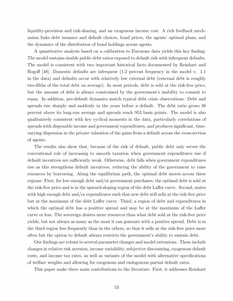
liquidity-provision and risk-sharing, and an exogenous income cost. A rich feedback mech-

anism links debt issuance and default choices, bond prices, the agents’ optimal plans, and

the dynamics of the distribution of bond holdings across agents.

A quantitative analysis based on a calibration to Eurozone data yields this key finding:

The model sustains sizable public debt ratios exposed to default risk with infrequent defaults.

The model is consistent with two important historical facts documented by Reinhart and

Rogoff [48]: Domestic defaults are infrequent (1.2 percent frequency in the model v. 1.1

in the data) and defaults occur with relatively low external debt (external debt is roughly

two-fifths of the total debt on average). In most periods, debt is sold at the risk-free price,

but the amount of debt is always constrained by the government’s inability to commit to

repay. In addition, pre-default dynamics match typical debt crisis observations: Debt and

spreads rise sharply and suddenly in the years before a default. The debt ratio grows 38

percent above its long-run average and spreads reach 953 basis points. The model is also

qualitatively consistent with key cyclical moments in the data, particularly correlations of

spreads with disposable income and government expenditures, and produces significant, time-

varying dispersion in the private valuation of the gains from a default across the cross-section

of agents.

The results also show that, because of the risk of default, public debt only serves the

conventional role of increasing to smooth taxation when government expenditures rise if

default incentives are sufficiently weak. Otherwise, debt falls when government expenditures

rise as this strengthens default incentives, reducing the ability of the government to raise

resources by borrowing. Along the equilibrium path, the optimal debt moves across three

regions: First, for low enough debt and/or government purchases, the optimal debt is sold at

the risk-free price and is in the upward-sloping region of the debt Laffer curve. Second, states

with high enough debt and/or expenditures such that new debt still sells at the risk-free price

but at the maximum of the debt Laffer curve. Third, a region of debt and expenditures in

which the optimal debt has a positive spread and may be at the maximum of the Laffer

curve or less. The sovereign desires more resources than what debt sold at the risk-free price

yields, but not always as many as the most it can generate with a positive spread. Debt is in

the third region less frequently than in the others, so that it sells at the risk-free price more

often but the option to default always restricts the government’s ability to sustain debt.

Our findings are robust to several parameter changes and model extensions. These include

changes in relative risk aversion, income variability, subjective discounting, exogenous default

costs, and income tax rates, as well as variants of the model with alternative specifications

of welfare weights and allowing for exogenous and endogenous partial default rates.

This paper make three main contributions to the literature. First, it addresses Reinhart

53

and Rogoff’s “forgotten history of domestic debt” by providing a framework that explains

outright defaults on domestic public debt. Second, debt, default and spreads are driven by

a feedback mechanism in which social welfare incorporates the utility of domestic bond and

non-bond holders, and debt has social value for self-insurance, liquidity, and risk-sharing,

instead of by the value of consumption smoothing for a representative agent, as in standard

external default models. Third, realistic debt, default, and spread dynamics are obtained,

relying on endogenous default costs due to the social value of debt and without exclusion

from credit markets beyond the default period, while external default models often rely

heavily on exogenous default costs and credit-market exclusions of stochastic length.

The literature on domestic sovereign default is at an early stage. Some important topics

to consider for future research include adding a richer structure of saving vehicles in the form

of real and financial assets, complementing debt and default choices with an optimal choice

of distortionary taxes, and adding secondary debt markets.

54

References

[1] Aguiar, M., and M. Amador (2016) “Fiscal Policy in Debt Constrained Economies,”

Journal of Economic Theory, 161, pp 37-75.

[2] Aguiar, M., and M. Amador (2014) “Sovereign Debt,” Handbook of International Eco-

nomics, 4, pp 647-87.

[3] Aguiar, M., M. Amador, E. Farhi, and G. Gopinath (2015) “Coordination and Crisis in

Monetary Unions,” Quarterly Journal of Economics, 130, pp 1727-1779.

[4] Aguiar M., S. Chatterjee, H. Cole, and Z. Stangebye (2016) “Quantitative Models of

Sovereign Debt Crises,” forthcoming Handbook of Macroeconomics Vol II.

[5] Aguiar, M., and G. Gopinath (2006) “Defaultable debt, interest rates and the current

account,” Journal of International Economics, 69(1), pp 64-83.

[6] Aiyagari, R., and E. McGrattan (1998) “The Optimum Quantity of Debt, ” Journal of

Monetary Economics, 42, pp 447-469.

[7] Andreasen, E., G. Sandleris, and A. Van der Ghote “The Political Economy of Sovereign

Defaults,” Universidad Torcuato Di Tella, Business School Working Paper, 2011-07.

[8] Arellano, C. (2008) “Default Risk and Income Fluctuations in Emerging Economies,”

American Economic Review, 98(3), pp 690-712.

[9] Arellano, C., Y. Bai, and L. Bocola (2017) “Sovereign default risk and firm heterogene-

ity” National Bureau of Economic Research, (No. w23314).

[10] Arslanalp, S. and T. Tsuda (2014) “Tracking Global Demand for Advanced Economy

Sovereign Debt” IMF Economic Review, 62(3), pp 430-464.

[11] Azzimonti, M. E. de Francisco, and V. Quadrini (2014) “Financial Globalization, In-

equality, & the Rising Public Debt,” American Economic Review, 104(8), pp 2267-2302.

[12] Bai, Y. and J. Zhang (2010), ”Solving the Feldstein-Horioka Puzzle with Financial

Frictions,” Econometrica, v. 78, no. 2, pp. 603-632.

[13] Bhandari, A., D. Evans, M. Golosov, and T. Sargent (2017) “Public Debt in Economies

with Heterogeneous Agents,” forthcoming Journal of Monetary Economics.

[14] Bocola, Luigi (2016) “The Pass-Through of Sovereign Risk,” Journal of Political Econ-

omy, Vol 124(4), pp 879-926.

[15] Broner F., A. Martin, and J. Ventura (2010) “Sovereign Risk and Secondary Markets,”

American Economic Review, 100(4), pp 1523-1555.

[16] Chang, B.H., Chang, Y, and S. Kim, (2015), “Pareto Weights in Practice: Income

Inequality and Tax Reform,” Working Paper No. 590, Rochester Center for Economic

Research, University of Rochester.

[17] Chatterjee, S., and B. Eyigungor (2012) “Maturity, Indebtedness, and Default Risk,”

American Economic Review, 102(6), pp 2674-99.

55

[18] Conesa J.C. and T. Kehoe (2005) “Productivity, Taxes and Hours Worked in Spain:

1970−2003,” Manuscript, University of Minnesota.

[19] Corbae, D., P. D’Erasmo, and B. Kuruscu (2009) “Politico-Economic consequences of

rising wage inequality,” Journal of Monetary Economics, 56(1), pp 43-61.

[20] Cuadra G., Sanchez J. and Sapriza H. (2010) “Fiscal Policy and Default Risk in Emerg-

ing Markets,” Review of Economic Dynamics, 13(2), pp 452-469.

[21] D’Erasmo P. and E. Mendoza (2016) “Distributional Incentives in an Equilibrium Model

of Domestic Sovereign Default,” Journal of the European Ec. Assoc., Vol 14 (1), pp 7-44.

[22] Dias D., C. Richmond, and M. Wright (2012) “In for a Penny, in for a 100 Billion

Pounds: Quantifying the Welfare Benefits from Debt Relief,” mimeo.

[23] Di Casola, P. and S. Sichlimiris (2018) “Domestic and External Sovereign Debt,”

Sveriges Riksbank Working Paper No. 345.

[24] Dovis, A., M. Golosov and A. Shourideh (2016) “Political Economy of Sovereign Debt:

A Theory of Cycles of Populism and Austerity,” NBER wp21948.

[25] Du, W. and J. Schreger (2016) “Sovereign Risk, Currency Risk, and Corporate Balance

Sheets,” mimeo.

[26] Eaton J. and M. Gersovitz (1981) “Debt with Potential Repudiation: Theoretical and

Empirical Analysis,” Review of Economic Studies, 48(2), pp 289-309.

[27] Floden M. (2001) “The effectiveness of government debt and transfers as insurance,”

Journal of Monetary Economics, 48, pp 81-108.

[28] Fuchs-Schundeln, N., D. Krueger, and M. Sommer (2010) “Inequality trends for Ger-

many in the last two decades: A tale of two countries” Review of Economic Dynamics,

13, pp 103−132.

[29] Gennaioli N., A. Martin and S. Rossi, (2014) “Sovereign default, domestic banks and

financial institutions,” Journal of Finance, 69(2), pp 819-866.

[30] Guembel A. and O. Sussman (2009) “Sovereign Debt without Default Penalties, ” Re-

view of Economic Studies, 76, pp 1297-1320.

[31] Guvenen, F (2009) “An Empirical Investigation of Labor Income Processes,” Review of

Economic Dynamics, 12(1), 58-79.

[32] Jappelli, T. and L. Pistaferri (2010) “Does consumption inequality track income in-

equality in Italy?” Review of Economic Dynamics, 13, pp 133−153.

[33] Jeon, K. and Z. Kabukcuoglu (2014) “Income Inequality and Sovereign Default”, work-

ing paper, University of Pittsburgh.

[34] Hall, G., and T. Sargent (2014) “Fiscal Discrimination in Three Wars,” Journal of

Monetary Economics, 61, pp 148−166.

56

[35] Hatchondo, J.C., and L. Martinez (2009) “Long-duration bonds and sovereign defaults,”

Journal of International Economics, vol. 79(1), pp 117−125.

[36] Heathcote J. (2005) “Fiscal Policy with Heterogeneous Agents,” Review of Economic

Studies, 72, pp 161-188.

[37] Heathcote, J., K. Storesletten, and G. Violante (2009) “Quantitative macroeconomics

with heterogeneous households,” Annual Review Economics, 1, pp. 319354.

[38] Heathcote, J., K. Storesletten, and G. Violante (2016) “Optimal Tax Progressivity: An

Analytical Framework,” Federal Reserve Bank of Minneapolis, Staff Report 496.

[39] D. Krueger, K. Mitman, and F. Perri (2016) “Macroeconomics and Household Hetero-

geneity” Handbook of Macroeconomics. Vol. 2., 2016. pp. 843-921.

[40] Lojsch D., M. Rodriguez-Vives and M. Slavik (2011) “The size and composition of

government debt in the euro area,” Occasional Paper Series 132, E.C.B..

[41] Mendoza, E. G., Tesar, L. L., and Zhang, J. (2014) “Saving europe?: The unpleasant

arithmetic of fiscal austerity in integrated economies” NBER, wp20200.

[42] Mengus E. (2014) “Honoring Sovereign Debt or Bailing Out Domestic Residents? A

Theory of Internal Cost of Default,” WP Banque de France 480.

[43] Olivares-Caminal, R. (2013)“The Pari Passu Clause in Sovereign Debt Instruments:

developments in recent litigation,” Proceedings from Sovereign Risk: A World Without

Risk-Free Assets? Bank for International Settlements.

[44] Paczos, W., and K. Shakhnov (2018) “Sovereign debt issuance and selective default.”

European University Institute, mimeo.

[45] Panizza, U., F. Sturzenegger and J. Zettelmeyer (2009) “The Economics and Law of

Sovereign Debt and Default,” Journal of Economic Literature, 47(3), pp 651-98.

[46] Perez, D. (2015) “Sovereign Debt, Domestic Banks and the Provision of Public Liquid-

ity,” Manuscript, New York University.

[47] Pijoan-Mas, J., and V. Sanchez-Marcos (2010) “Spain is Different: Falling Trends of

Inequality,” Review of Economic Dynamics, 13(1), pp 154-178.

[48] Reinhart C., and S. Rogoff (2008) “The Forgotten History of Domestic Debt,” NBER

Working Papers 13946.

[49] Rojas, E. (2018) “Understanding Sovereign Default Costs: The Role of Firm Hetero-

geneity,” mimeo.

[50] Sosa-Padilla, C. (2014) “Sovereign Defaults and Banking Crises,” forthcoming Journal

of Monetary Econmics.

[51] Yue, V. (2010) “Sovereign Default and Debt Renegotiation,” Journal of International

Economics, 80(2), pp 176-87.

57