NAVAL POSTGRADUATE SCHOOL

Monterey, California

rc,=

ý~MAR 18 1994,THESIS BU

LINEAR QUADRATIC GAUSSIAN CONTROLLER DESIGNUSING LOOP TRANSFER RECOVERY

FOR A FLEXIBLE MISSILE MODEL

byFernando Jimenez

December, 1993

Thesis Advisor: Roberto Cristi

Approved for public release; distribution is unlimited.

;Q> 94-08758llll~~il!!llllltllliliill" B •

REPORT DOCUMENTATION PAGE Bom 074-ov18

Public reporting burden for theis collection of information is estimated to avefIge 1 hour per response including the lime for reviewing instructions searching existing data sourcesgathenng and maintaining the data needed, and completing and reviewing the collection of information Send comments regarding this burden estimate or any other aspect of thiscollection of information, including suggetlions for reducing this burden, to Washington Headquarters Services. Directorate for Information Operations and Reports 1215 Jefferson DavisHighway, Suite 1204. Arlington. VA 22202-4302 and to the Office of Management and Budget Paperwork Reduction Prolect (0704-0188) Washington. DC 20503

1. AGENCY USE ONLY (Leave Blank) 2. REPORT DATE 3. REPORT TYPE AND DATES COVERED

December 17, 1993

4. TITLE AND SUBTITLE 6. FUNDING NUMBERS

LINEAR QUADRATIC GAUSSIAN CONTROLLER DESIGN USING LOOP TRANSFERRECOVERY FOR A FLEXIBLE MISSILE MODEL

6. AUTHOR(S)Jimdnez, Fernando

7. PERFORMING ORGANIZATION NAMES (S) AND ADDRESS(ES) 8. PERFORMING ORGANIZATION

Naval Postgraduate SchoolMonterey, CA 93943-5000

9. SPONSORINGNMONITORING AGENCY NAME(S) AND ADDRESS(ES) 10. SPONSORING/MONITORINGAGENCY REPORT NUMBER

Naval Postgraduate SchoolMonterey, CA 93943-5000

11. SUPPLEMENTARY NOTES

12a. DISTRIBUTION/AVAILABILITY STATEMENT 12b. DISTRIBUTION CODE

Approved for public release, distribution is unlimited. A

13. ABSTRACT (Maximum 200 words)

In this thesis, a Linear Quadratic Gaussian Controller (LQG) is designed for a tail controlled surface-to-air missile model in order tomeet design specifications. The mathematical model of the flexible missile is subject to uncertainties that may arise from unmodelleddynamics, parameter variation or linearization of nonlinear elements. Since these uncertainties are not taken into account in the LQGcontroller, V Analysis is applied to the design in order to evaluate the Robust Performance. Robust Stability, and NominalPerformance of the system. Finally, a Linear Quadratic Gaussian controller is designed using Loop Transfer Recovery (LQGLTR) inorder to improve the Robust Stability of the system. It is found that the Robust Stability of the design is improved, but as aconsequence of losing nominal performance. The p Analysis and Synthesis Toolbox and the Control Toolbox of MATLAB were usedfor the design, assembly, analysis and simulation of the missile flight control system.

14. SUBJECT TERMS 16. PRICE CODE

Robust Multivariable Control, Linear Optimal Estimation, Missile Autopilot 15. NUMBER OF PAGES67

17. SECURITY CLASSIFICATION 18. SECURITY CLASSIFICATION 10. SECURITY CLASSIFICATION 20. LIMITATION OF ABSTRACTOF REPORT OF THIS PAGE OF ABSTRACT

UNCLASSIFIED UNCLASSIFIED UNCLASSIFIED UNLIMITED

NSN 7540-01-280-5500 Standard Form 298 (Rev. 2-89)Prescribed by ANSI Std. 239-18 298-102

Approved for public release; distribution is unlimited.

LINEAR QUADRATIC GAUSSIAN CONTROLLER DESIGN USING LOOPTRANSFER RECOVERY FOR A FLEXIBLE MISSILE MODEL

by

Fernando JimenezLieutenant, Peruvian Navy

BSEE, Naval Postgraduate School, 1993

Submitted in partial fulfillmentof the requirements for the degree of

MASTER OF SCIENCE IN ELECTRICAL ENGINEERING

from the

NAVAL POSTGRADUATE SCHOOLDecember, 1993/

Author:

Fer ndo.4imenez

Approved By: , ._Roberto Cristi, Thesis Advisor

"Harol8Tits, Second Reader

Michael A. Morg1, ChairmanDepartment of Electrical and Computer Engineering

ii

ABSTRACT

In this thesis, a Linear Quadratic Gaussian Controller (LQG) is designed for a tail

controlled surface-to-air missile model in order to meet design specifications. The

mathematical model of the flexible missile is subject to uncertainties that may arise from

unmodelled dynamics, parameter variation or linearization of nonlinear elements. Since

these uncertainties are not taken into account in the LQG controller, P Analysis is

applied to the design in order to evaluate the Robust Performance, Robust Stability, and

Nominal Performance of the system. Finally, a Linear Quadratic Gaussian controller is

designed using Loop Transfer Recovery (LQGLTR) in order to improve the Robust

Stability of the system. It is found that the Robust Stability of the design is improved, but

as a consequence of losing nominal performance. The p Analysis and Synthesis Toolbox

and the Control Toolbox of MATLAB were used for the design, assembly, analysis and

simulation of the missile flight control system.

Acaa: en For

SU ... : (• ±

*' .. - ,- . ,. -

M-.-i.

L! /'

4

TABLE OF CONTENTS

I. IN T R O D U C T IO N ............................................................... 1.

II B A C K G R O U N D ... .......................................................... .6 .

A. GENERAL FEEDBACK PERTURBATION MODEL .......................... 6

B. UNSTRUCTURED UNCERTAINTY MODEL ............................... 8

C. STRUCTURED UNCERTAINTY MODEL .................................. 10

D. STRUCTURED SINGULAR VALUE ....................................... 12

1. Singular V alue D ecom position ........................................... 12

2. The Principal G ains ................................................. . . 14

3 . T he Infi nity N orm ....................................................... 15

4. The Structured Singular Value ............................................ 16

III. LINEAR QUADRATIC GAUSSIAN (LQG) DESIGN .......................... 17

A . M ISSILE M OD EL ............................................ ........... . 17

B. AUTOPILOT DESIGN REQUIREMENTS .................................. 20

C . PRO PO SED D E SIG N ...................................................... 21

IV. p-ANALYSIS FOR LINEAR QUADRATIC GAUSSIAN DESIGN ............. 31

A. NOMINAL STABILITY AND ROBUST STABILITY ....................... 32

B. NOMINAL PERFORMANCE .............................................. 3.4

C. ROBUST PERFORMANCE ................................................ 35

V. LQG LOOP TRANSFER RECOVERY DESIGN (LQGLTR) ..................... 39

iv

VI. CONCLUSIONS AND RECOMMENDATIONS ....... ............... ... 53

A . S U M M A R Y ............................ ................................... 53

B . C O N C L U SIO N S ........................................................... 54

C. RECOM M END ATION S .................................................... 55

LIST O F REFEREN CES .......................................................... 56

INITIAL DISTRIBUTION LIST ............................................... 5.7

v

LIST OF FIGURES

Figure 1. General A-P-K Fram ework ................................................ 6

Figure 2. Unstructured Uncertainty M odels .......................................... 9

Figure 3. Closed Loop System with Feedback Perturbation .......................... 10

Figure 4. Model of the Tail Control Surface-to-Air Flexible Missile................... 18

Figure 5. Missile Response Due to a Unit Step Commanded Acceleration ............ 22

Figure 6. Closed Loop Optimal Output Feedback System ........................... 25

Figure 7. Achieved Normal Acceleration Due to a Unit Step Commanded

A cceleratio n ....................................................... ...... 2 6

Figure 8. Gyro Output Due to a Unit Step Commanded Acceleration ................. 27

Figure 9. Pitch Rate Due to a Unit Step Commanded Acceleration ................... 27

Figure 10. Angle of Attack Due to a Unit Step Commanded Acceleration ............. 28

Figure 11. Actual Fin Deflexion Due to a Unit Step Commanded Acceleration ....... 28

Figure 12. Fin Rate Due to a Unit Step Commanded Acceleration .................... 29

Figure 13. Linear Fractional Transformation ................................... . 32

Figure 14. Nominal Closed Loop Plant with a Feedback Perturbation ................. 33

Figure 15. Robust Performance, Robust Stability, Nominal Performance of

L Q G D esign ........................................................... 36

Figure 16. LQG Design Under Uncertainty Variations .............................. 37

vi

Figure 17. Optimal Linear Output Feedback Control System with Loop Broken at the

C o ntro l In p u t . ...................................................... . 4 1

Figure 18. Optimal Linear Output Feedback Control System with Feedback Perturbation

and Loop Broken at the Uncertainty ..................................... 42

Figure 19. General A-P-K Framework with Fictitious Noise Added at the Uncertainty 43

Figure 20. Nyquist Polar Plot for Optimal Control .................................. 45

Figure 21. Nyquist Polar Plot for Optimal Control Plus Kalman Filter ................. 46

Figure 22. Nyquist Polar Plot for Optimal Control Plus Kalman Filter ................ 47

Figure 23. Nyquist Polar Plot for Optimal Control Plus Kalman Filter .............. -48

Figure 24. Acceleration Time Response (a) and It-analysis (b) for LQG Design without

U ncertainties. .. ........................................................ 4 9

Figure 25. Acceleration Time Response (a) and pI-analysis (b) for LQG Design in the

Presence of an Uncertainty in Z ......................................... 50

Figure 26. Acceleration Time Response (a) and rt-analysis (b) for LQGLTR Design in the

Presence of an Uncertainty in Z,

(Variance of the Fictitious Noise =1) ..................................... 50

Figure 27. Acceleration Time Response (a) and pI-analysis (b) for LQGLTR Design in the

Presence of an Uncertainty in Za

(Variance of the Fictitious Noise= 100) ................................... 51

vii

Figure 28. Acceleration Time Response (a) and p-analysis (b) for LQGLTR Design in the

Presence of an Uncertainty in Za

(Variance of the Fictitious Noise=500) ................................... 52

viii

I. INTRODUCTION

Highly evasive target maneuver levels and increasingly effective electronic

countermeasures push current air defense missile systems to the limits, resulting in more

stringent autopilot performance requirements. Conventional autopilot design techniques

have worked well in the past, but new design methods are required to obtain improved

performance and robustness characteristics from the flight control system in order to

satisfy future design specifications. A significant research effort has been directed toward

the design and implementation of robust controllers which can guarantee both stability

and performance

Robust control design methods such as H, Optimal control or Linear Quadratic

Gaussian Loop Transfer Recovery optimize performance and stability based on

engineering models which include performance specifications and descriptions of how

uncertainty modifies the nominal plant.

Recent advances in robust feedback control, in particular H, control and

p.-synthesis, allow for new design methodologies to be applied to the design of missile

flight control systems. IL, optimal control provides the basis for controller synthesis

while mu analysis characterizes performance and stability in the presence of a defined

structure for uncertainties. Recent advances in robust control theory offer good prospects

for meeting the design needs of next generation missiles. Several anticipated benefits of

I

the robust control design appoach are- greater flexibility in the choice of airframe

geometry, full use of available airframe maneuver capability and greater tolerance to

uncertainty in design models.

Linear quadratic controllers using state estimate feedback are optimal for the

nominal model but the performance may be far from satisactory in a real life situation in

which the plant differs somewhat from the model. Attractive passband robustness

properties of full-state feedback optimal quadratic designs may disappear with the

introduction of a state estimator. The Linear-Quadratic-Gaussian with

Loop-Transfer-Recovery (LQG/LTR) methodology provides an integrated frequency

domain and state approach for design of multi-input multi-output (MIMO) control

systems. The advantages of the methodology lie in its ability to directly address design

issues such stability robustness and the trade-off between performance and allowabie

control power.

In this study the problem of the design of a pitch plane autopilot to track normal

accelerations commanded from the guidance system for a tail controlled flexible missile

[Ref 1 ] using Linear Quadratic Gaussian techniques is presented.

In general when a missile is flying at an angle of attack alpha, lift is developed

This lift may be represented as acting at the center of pressure of the structure. The missile

will be statically stable or unstable without corrective tail deflections depending on the

location of the center of pressure relative to the center of mass.

2

The control problem requires that the autopilot generate the required tail-deflection

delta to produce an angle of attack, corresponding to a maneuver called for by the

guidance law, while stabilizing the airframe rotational motion. The primary objective of

the missile autopilot is to control the missile's flight path while meeting the specified

performance requirements and to mantain the specified stability margins of the airframe

over the entire flight envelope, all in the presence of parameter variations, unmodeled

dynamics and disturbances. The missile flight control system must guarantee stability

and performance in the face of large aerodynamic uncertainties and disturbances. This

requires the feedback controller to maintain system stability and loop performance for all

variations in the plant behavior. The autopilot design goals are simply to make the missile

respond as fast as possible while maintaining stability. Stability robustness goals include

robustness to neglected bending dynamics and uncertainties in the aerodynamic

parameters.

A pitch plane model describing the longitudinal dynamics of the missile is available

for this design. Reasonable accurate mathematical models of the rigid body transfer

functions from tail-deflection to the sensor outputs are available too. Sensor

measurements for feedback include missile rotational rates (from a rate gyro) and normal

acceleration (from an accelerometer).

The sensors are assumed to be subjected to noises, dynamic characteristics,

calibration errors and drifts.

3

The mathematical model of the flexible missile is subject to uncertainties thatmay

arise from unmodeled dynamics, parameter variation, linearization of nonlinear elements.

Model perturbations or uncertainties such as aerodynamic stability coefficient variation

uncertainties and actuator perturbations are considered in the model. Multiplicative

parameter uncertainties are considered upon the pitching moment and normal force

aerodynamic stability derivatives with respect to angle of attack.

In general there are other uncertainties associated with a missile system that can be

considered but are not part of this specific model. For example, the missile may be

constantly subjected to environmental disturbances such as wind gust. The wind may

induce a sideslip excursion and affect the measurements.

The problem of structural flexibility is also taken into account since this is a long

and slender missile. This introduces problems relating to the elastic nature of the airframe.

As the autopilot bandwidth increases, coupling between the flight control system and the

flexible dynamics of the airframe may take place which limits the achievable airframe

response and possibly destabilizes the system. Coupling occurs between the elastic modes

and the control system as the control system gyros and accelerometers sense the flexure

motion and the rigid body motion. The coupling arises from the fact that the attitude and

rate gyros and accelerometers sense both the rigid body changes and the body bending

motion.

The controller must avoid saturating the tail deflection actuator rate capabilities and

destabilizing high frequency flexible body modes of the missile. The push for a smaller

4

time constant to achieve a rapid command response is in conflict with the requirement for

robust stability against high frequency uncertain dynamics. During flight, aerolastic

forces also act on the airframe, causing high-frequency vibratory modes. The vibrations

affect both the acceleration and the pitch rate but only the second one is considered in the

model of the missile.

This work is organized as follows. Robust multivariable control theory as well as

the Structured Singular Value will be introduced in Chapter II. The Structured Singular

Value will play -.. nportant role in the evaluation of the missile's performance in

Chapter IV. Linear Quadratic Gaussian techniques will be applied to the missile model in

Chapter III to yield the desired specifications. This chapter also presents the missile and

airframe models used in the design. A technique known as pi analysis is applied in Chapter

IV in order to evaluate Robust Performance, Robust Stability and Nominal Performance

of the Linear Quadratic Gaussian design for the model of the missile. Linear Quadratic

Gaussian with Loop Transfer Recovery is applied in Chapter V to improve the stability

robustness of the system. The final chapter summarizes the results and suggest further

research.

5

H. BACKGROUND

A. GENERAL FEEDBACK PERTURBATION MODEL

Any general feedback system in the presence of uncertainties can be represented by

the general A-P-K framework shown in Figure 1, where the plant model P(,) has been

expanded to include additional input and output variables.

Wd Yd

w 'mY

u m

P Plant ModelA UncertaintyK Feedback Compensator

W Disturbance InputWd Feedback through uncertaintyYd Output Leading to feedback uncertaintyY Reference output

Figure 1. General A-P-K Framework.

6

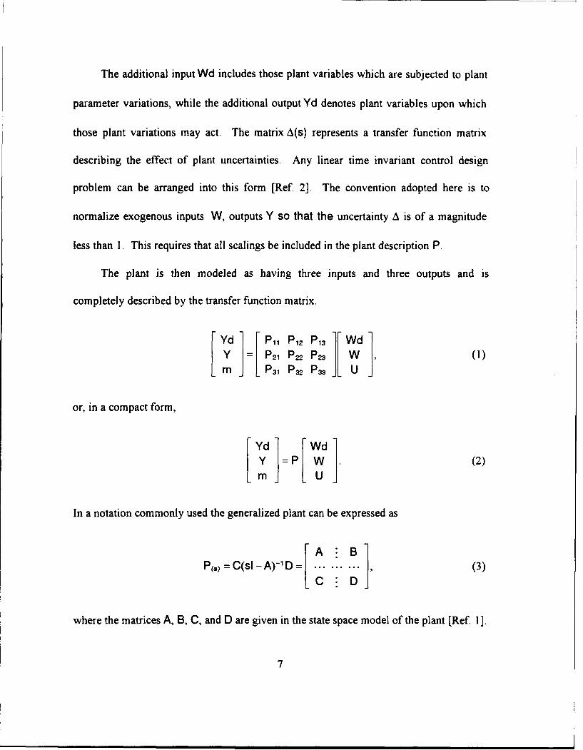
The additional input Wd includes those plant variables which are subjected to plant

parameter variations, while the additional output Yd denotes plant variables upon which

those plant variations may act. The matrix A(s) represents a transfer function matrix

describing the effect of plant uncertainties. Any linear time invariant control design

problem can be arranged into this form [Ref. 2]. The convention adopted here is to

normalize exogenous inputs W, outputs Y so that the uncertainty A is of a magnitude

less than 1. This requires that all scalings be included in the plant description P.

The plant is then modeled as having three inputs and three outputs and is

completely described by the transfer function matrix.

Yd 11 P12 P13 Wd

m P31 P32 P33 U

or, in a compact form,

Yd WdY = P W (2)m U

In a notation commonly used the generalized plant can be expressed as

P(.) = C(sl - A)-' D =. (3)C : D

where the matrices A, B, C, and D are given in the state space model of the plant [Ref. 1].

7

B. UNSTRUCTURED UNCERTAINTY MODEL

A linear model of a multivariable linear system includes a description of the

uncertainties and their structure. The uncertainties are due to parameter variations,

unmodeled dynamics, neglected flexible body dynamics, non-linearities, and various

assumptions that affect the model of the real system [Ref. 1].

In general, uncertainties in dynamic models could enter the system in a variety of

ways, such as parametric or non-parametric, structured or unstructured, stochastic or

deterministic.

An unstructured uncertainty is modeled as an unknown with a bounded transfer

function incorporated in series or parallel with the plant [Ref. 3]. This type of model of

the plant uncertainty is termed unstructured since no detailed model of the perturbation is

employed. Figure 2 shows the unstructured uncertainty models that will be considered.

The actual plant will equal the nominal plant for each of these cases when the

perturbation equals zero. For evaluation of stability, robustness or performance

robustness these perturbations are assumed to be contained within bounds.

M (4)

Additive

AO(s)+

G(s)

Input Multiplicative

G0(s rpresen s)tenmna ln

GO(s)

Output Multiplicative

A(s)G(s)

whereG0(s) represents the nominal plant

x(s) represents a perturbation

Figure 2. Unstructured Uncertainty Models.

9

C. STRUCTURED UNCERTAINTY MODEL

Structured uncertainties refer to plants which contain one or more uncertain

parameters; they also refer to plants which contain both uncertain parameters and

unstructured uncertainties.

Uncertain blocks and parameters from various plant locations can be rearranged as

shown in Figure 3 [Ref. 3].

Wd t AA L Yd

w Y

Figure 3. Closed Loop System with Feedback Perturbation.

In this figure M(s) is the combination of the nominal plant P(s) with a feedback

compensator K(s), and it represents the dynamics of the nominal closed loop system. It

can be divided into 4 blocks as shown below [Ref. 1].

M=F Mil M12 (5)L M 21 M22 '

relative to the inputs and outputs

10

This matrix partition is called Linear Fractional Transformation and is derived from

the following linear equations.

Y M W (6)

The term M 2 may be viewed as the nominal closed loop dynamics, assuming no

uncertainties and A as a linear-fractional uncertainty. The matrices M,,, M12, M21, F (M,

A) describe how A affects the overall dynamics, expressed by the transfer function matrix

F(M, A) = M2 +M 21 A(I - M 11 A)-1 M 12 (7)

We assume independence of the terms in the structured perturbation whith is of the

form

AI(s) 0 - 0

A(s) 0 A2(s) 0 (8)

0 0 Ap(s)

or, more compactly

A =diag{A, A2 , ... Ap) (9)

The individual uncertainties, AP that make up the A block may have one of several

representations [Ref. I]:

11

1 Scalar Block; uncertainty appears only once in the real system, such as

parameter uncertainty.

2. Repeated Scalar Blocks; where the uncertainty appears multiple time in real

system.

3. Full Blocks; example of which includes multivariable neglected dynamics and

the performance block.

As in the standard model for unstructured uncertainties, the structured uncertainties

will all be scaled so their infinity norms equal one [Ref. 3]

1I 11. I= 1AII. =... = IIAPIIL = 1. (10)

where we define the infinity norm as IAlll., =sup •[A(jco)].w

D. STRUCTURED SINGULAR VALUE

1. Singular Value Decomposition

Any m x n matrix can be factored as

A=V-U T (11)

where V is an m x m orthogonal matrix, U is an n x n orthogonal matrix, 7 is an m x n

matrix of the special form Do 0(12)

0 0

12

where

0, 0 -D.L j (13)

0 CykJ

is diagonal.

The elements a1 > a 2 >.. -> a_ > 0 are all positive real, and are called the singular

values of the matrix A. The singular decomposition has the property that the L, gain of

the matrix lies between the smallest and the largest singular values.

jUx II

T=a <Yý- :!:- <r a =(14)

where a_ is the smallest singular value and d is the largest singular value.

For SISO systems the concept of "gain" is synonymous with the classical Bode

magnitude plot. This Bode magnitude is equal to the amount of amplification of a

sinusoidal input by the system.

For multivariable systems, the extension of the Bode gain is the singular value of

a transfer matrix M evaluated at a frequency upon the imaginary axis, M(jo) [Ref. 4].

If we consider the transfer function matrix M evaluated at any frequency point

M(jco), the largest amplification that a sinusoidal signal of frequencycO will receive as it

passes through M is equal to the maximum singular value of M at s = jco.

13

2. The Principal Gains

The principal gains are the frequency dependent singular values of the system

They can be used to assist the designer in determining the robustness of the multivariable

system and are a good indicator of the system's ability to cope with disturbance rejection-

The principle gains will be denoted as [Ref. 5]

c;(Gjco) = y (15)

where G(jco) is the frequency dependent transfer function of the system.

If the principal gains of the transfer function matrix of the MIMO system are

ordered such that

Y1 <Y2 < ... <Yn, (16)

then yand yn have the property that they bound the L. gain between the disturbance input

vector d(s) and the output vector y(s)

YI1-<Yn (17)

Thus if yn is determined for the transfer function matrix then this is the maximum

gain which can be obtained by any disturbance vector d(s) and gives a worst case

indication of the disturbance rejection properties of the control system while Y, gives an

indication of the best rejection by the system.

14

Large values ofoa,, over a large range of frequencies result in good tracking of

reference inputs and good rejection of disturbances.

The maximum gain of the system will be denoted by

•(Gdji)) (18)

and the minimum gain by

o_(Goc•)) (19)

The maximum gain that a stable linear system M can deliver is then the

supremum of the maximum singular values taken over all frequencies.

3. The Infinity Norm

Mathematically, the infinity norm of a transfer function matrix M is defined as

the supremum over all frequencies of the maximum singular valued of M(jco).

It is denoted by

IIM1I. =sup a[M(jo)] (20)

W

The first engineering relevance of the infinity norm is that if a control designer

seeks to design a controller K for minimizing the transfer of energy or the transfer of

power or the transfer of white noise through a closed loop system M which depends on K,

then the controller K should be designed so that the infinity norm M, fIMII,, is minimized

over all controllers which stabilize the closed loop system M.

15

The second engineering relevance of the infinity norm is that it is essential in

establishing robustness of uncertain systems.

4. The Structured Singular Value

The structured singular value of a complex matrix M denoted by It(MO(o)), with

respect to the block structured A, is based on the multivariable Nyquist Theorem and is

defined as

ýLMO (21)min [(A)" det(I + MA(jco)) = 0AEA3

where A denotes the set of all transfer function matrices with the appropriate block

diagram form.

It can be shown that the structured singular value is the inverse of the stability

margin for multivariable systems [Ref. 3]. In other words, M is the inverse of the smallest

magnitude of a destabilizing perturbation of M.

The structured singular value is a measure of robustness of the model, to

structured perturbations.

The structured singular value provides an indication of how much uncertainty

can be tolerated before the systems becomes unstable. It will be used in Chapter IV in

order to evaluate the robust performance and robust stability of the Linear Quadratic

Guassian design for the missile model proposed in Chapter III.

16

M. LINEAR QUADRATIC GAUSSIAN (LQG) DESIGN

In this chapter we apply LQG techniques to the design of a controller for the model

of a missile with flexible modes proposed in Section A, in order to meet design

requirements specified in Section B.

A. MISSILE MODEL

The airframe model used in this thesis was presented by Bibel [Ref. 1]. A block

diagram configuration for the model of the surface launched, antiair homing missile to be

considered is shown in Figure 4. The missile is formed basically by the following

sub-systems: fin actuator, rigid body dynamics, rate gyro, accelerometer, and flexible

body dynamics. The State Space Model representation of this Multi-Input Multi-Output

System can be described by

k = Ax + Bu + W, (22)

y = Cx + Du + TfV, (23)

where

A = Plant Matrix, B = Input Matrix, C = Output Matrix, D = Feedforward Matrix,

[ = Input Matrix, T =Measurement Noise Input Matrix.

17

N

L) >-

N0

0))

'9)

0)

NN

04)

CO)

The reference input to the system is given by the commanded acceleration and the

control input is given by the commanded fin deflection. Two disturbances entering the

system, accelerometer bias and gyro drift, and two measurements, measured acceleration

error and measured pitch, are modelled as white noise processes with intensities W and

V, respectively.

V V(t) V 1 (t) V 2Mtý o(41V2 ( ) t to , (24)

where V,(t) and V2(t) are the intensity of W and V, respectively and are correlated.

V, 2(t) is equal to 0 (uncorrelated) and W and V are independent.

We define the covariance matrices as

E[W(t)WI(t + T)] = 06(t - T), (25)

E[V(t)VI(t + -")] = R5(t - r). (26)

For the purpose of modeling these two disturbances, models for biases have been

added to the nominal plant model. The error between the commanded acceleration and

the measured normal acceleration and the measured body pitch rate are the feedback

signals to the controller.

The state variables considered in the nominal model are summarized in Table I.

19

TABLE 1. NOMINAL MODEL STATE VARIABLES ANDPARAMETERS.

Fin Rate

6 Actual Fin Deflection

aX Angle of Attack

q Pitch Rate

Commanded Fin Deflection

*1Normal Acceleration (measured by theaccelerometer)

TIC Commanded Acceleration

TERROR Error between rin and rT

im Measured Acceleration

ql, Measured Pitch Rate

em n Measured error in Acceleration

The model to be considered in the design of the linear quadratic gaussian controller

combines the nominal plant and the process-noise model but does not include the

description of the uncertainties and their structure (i.e., two aerodynamic stability

coefficient variation uncertainties, two actuator perturbations, multiplicative parameter

uncertainties on the pitching moment, and normal force aerodynamic stability derivatives

with respect to the angle of attack).

B. AUTOPILOT DESIGN REQUIREMENTS

The primary objective for the design of the autopilot is to obtain the fastest time

response possible while maintaining stability robustness. The following time domain

20

specifications are to be considered in the design of the linear quadratic gaussian controller

for the missile autopilot.

Settling Time Ts < 0.4 secs (Time constant = 0.1 secs)

Steady State Error e,, = 0.1 % (Due to a step command)

Overshoot Ov _ 4% (Due to a step command)

The linear quadratic gaussian controller has to be able to handle the effects of the

airframe's elastic dynamics.

C. PROPOSED DESIGN

The design of the linear quadratic gaussian controller for the model of this missile is

given by a combination of the solutions of the Stochastic Optimal Regulator and

Optimal Estimator problem.

The optimal control, solution of the stochastic optimal regulator problem, which

minimizes the next performance index

J =J 0 y 2(t) + pU 2(t)dt, (27)

where y(t) represents the output of the accelerometer and u(t) the control input to the

system is given by state feedback

u = -Kfx (28)

Kf = R-'B'P (29)

21

where P is the unique positive definite matrix satisfying the Matrix Riccati Equation

PA + ATP- PBR- 1BIP + Q = O (30)

provided that Q is symmetric and positive semidefinite, R is symmetric and positive

definite, the pair (A,B) is controllable, with the controllability matrix given by

S=[BABA 2B...A"-'B] (31)

The scalar p plays the role of a Lagrange multiplier. Asp decreases, the integrated

square regulating error decreases, but the integrated square input increases. From

simulation, p was chosen to be 0.1. The response of the missile due to a unit step

commanded acceleration with the Linear Quadratic Regulator is shown in Figure 5.

0.8 Pho=0.1

0.6-

00.4

0.2

0

0 0.1 0.2 0.3 0.4 0.5Time (secs)

Figure 5. Missile Response Due to a Unit Step Commanded Acceleration.

The solution of the Optimum Observer or State Estimator given by Kalman and

Bucy can be expressed by the following Differential Equation

22

i =AS(+ Bu + Ko(y - Ci). (32)

The Kalman Gain K. is optimally chosen so as to minimize

E {e (t)W(t)e(t)), (33)

and is given by

Ko(t) = -P.(t)C(t)R-1 (t), (34)

where P.(t) is the solution of the matrix Ricatti equation

0.(t) = P.(t)F'(t) + F(t)P.(t) - P.(t)H(t)R-1 (t)H'(t)P.(t) + Q(t), (35)

where

e(t) = x(t) - X^(t), (36)

and

F.(t) = F(t) + Ko(t)H/(t). (37)

This has a solution provided that

W is symmetric and Positive Semidefinite

V is symmetric and Positive Definite

The pair (A,C) is observable

where the observability matrix is given by

23

'g = [C T ATC T A 2CT. .ATWICT] (38)

The optimal output feedback control system is represented below. This combines

the model of the nominal plant with the optimal feedback gain and the optimal estimator.

It also includes a state command matrix N. that defines the desired value of the state, x,.

Since this is a tracking problem, N. should transform the reference input r to a reference

state. It can be shown that N,, can be calculated from the following matrix equation:

where D and [ represent the plant matrix and input matrix of the discrete representation

of the model of the system.

The Reference State is given by

x, = Nxr (40)

and it represents the state we want to track.

Equations (22), (28), (32), and (40) can be combined in order to obtain the State

Space Model for the Closed Loop Optimal Output Feedback System shown in Figure 6.

From the Control Law given by

u = XK(- X,), (41)

and substituting Equation (41) into Equation (22) we obtain the closed loop dynamics

24

* = Ax- BKf( -x,) + -W. (42)

ACCNOISE GYRONOISE

x=Ax+Bu+ry=Cx +Du,+V

Missile Model

+ ~x"= Ax + Bu + Ko(y,-cx)

Optimal XKalman FilterFeedback State CommandGain Nx Matrix

Cmdacc

Figure 6. Closed Loop Optimal Output Feedback System.

which can be written as

Ax -BKf + BKfx, + "W. (43)

25

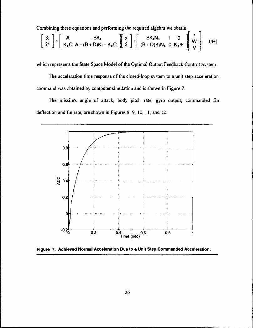
Combining these equations and performing the required algebra we obtain

[~=K A(B -B..K, x] [ BKtN,, 1 0 (44)x-X/= +W (44)x KoC A - (B + D)K, - KoC. (B +D)KfNx 0 KoT V

which represents the State Space Model of the Optimal Output Feedback Control System.

The acceleration time response of the closed-loop system to a unit step acceleration

command was obtained by computer simulation and is shown in Figure 7.

The missile's angle of attack, body pitch rate, gyro output, commanded fin

deflection and fin rate, are shown in Figures 8, 9, 10, 11, and 12

1

0.6 .. ...

0 0.4 .

0.2 .

-2•

-0. 0.2 0.4 0.6 0.8 1Time (sec)

Figure 7. Achieved Normal Acceleration Due to a Unit Step Commanded Acceleration.

26

01

0 .5,

0.2 0.4 0.6 0.8Time (sec)

Figure 8. Gyro Output Due to a Unit Step Commanded Acceleration.

15

"I-0.5

p I I

0 0.2 0 4 Time (sec) 0.6 0.8

Figure 9. Pitch Rate Due to a Unit Step Commanded Acceleration.

27

0.15

0.1-I-z

0.05

0.2 0.4 0.6 0.8Time (sec)

Figure 10. Angle of Attack Due to a Unit Step Commanded Acceleration.

0.04ZP•0.020 -

-0.02

0I I I I

0 0.2 0.4 0.6 0.8Time (sec)

Figure 11. Actual Fin Deflexion Due to a Unit Step Commanded Acceleration.

28

5.

0

z-10

-15

0 0.2 0.4 0.6 0.8 1Time (sec)

Figure 12. Fin Rate Due to a Unit Step Commanded Acceleration.

The following time domain specifications were achieved with a standard LQG design:

Final Value 1.0000 unit

Time to Peak 0.4500 secs

% Overshoot 0.0000 %

Rise Time 0.2500 secs

Settling Time 0.4000 secs

Steady State Error 0.0000 units

These specifications were obtained from Figure 7. The acceleration response is

critically damped and is the fastest that can be obtained for this particular design.

If we observe the missile's angle of attack and body pitch rate responses it can be

noticed that these two do not affect the flexible body dynamics. The fin deflection limit

of 40 degrees and the fin rate limit of 300 degrees/sec are not exceeded.

29

So far all of the required specifications for which the controller was designed have

been met, but we still have to check the stability of the system. The LQG controller was

designed for the nominal plant model of the missile and may or may not meet robust

stability requirement.

In the next chapter this design will be tested using a technique called p-analysis

which evaluates the robust performance, robust stability and nominal performance of the

design.

30

IV. p-ANALYSIS FOR LINEAR QUADRATIC GAUSSIAN DESIGN

The goal of any controller design is that the overall system is stable and satisfies

desired performance requirements. These requirements should be satisfied at least when

the controller is applied to the nominal plant, that is, nominal stability and nominal

performance is required. In practice the real plant is not equal to the model. Even though

there are uncertainties in the dynamics of any real system we try to quantify the

unmodeled dynamics.

In the design of the Linear Quadratic Gaussian controller, the nominal plant model

of the flexible missile was assumed to be known exactly. This is rarely the case due to

unmodeled dynamics, parameter variations, uncertainties, etc. Even if these uncertainties

are neglegible, it may be desirable to design a controller for a plant whose parameters

vary deterministically as a consequence of environmental factors or component failures.

When the controller designed for a nominal plant model is implemented on the real

system, there are no guarantees on the resulting performance of the system. Even

requirements as basic as stability may not be met. The deviation from the expected

behavior of the system clearly depends on the accuracy of the model. Because models are

never perfect, robustness analysis is necessary to determine the possibility of instability or

inadequate performance in the face of uncertainty of the plant dynamics. A controller

should guarantee stability, proper response to commands, and reduction of response

31

perturbations caused by disturbance inputs. Ability to perform the first function under

parameter variation is called stability robustness, while ability to conduct the remaining

two functions is termed performance robustness.

A. NOMINAL STABILITY AND ROBUST STABILITY

If the LQG controller is included in the nominal plant P, the following class of

general matrix transformation called Linear Fractional Transformation can be defined

as [Ref. 4]

F(P, K) = P11 + P 12 K(I - P 22 K)-1 P 21 (45)

F(PK) denotes the transfer function from W ] to [ Yd This particular structure is

shown in Figure 13.

Yd Wd14 Yd Wd

e P ey u

Figure 13. Linear Fractional Transformation.

32

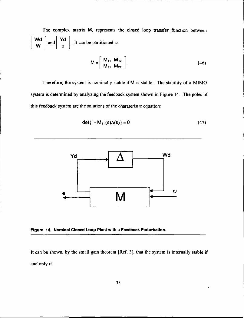
The complex matrix M, represents the closed loop transfer function between

[Wd ]and[ Yda]. It can be partitioned as

M ]1 1 (46)M 21 M 22"

Therefore, the system is nominally stable if M is stable. The stability of a MIMO

system is determined by analyzing the feedback system shown in Figure 14. The poles of

this feedback system are the solutions of the charateristic equation:

det{I + M1. (s)A(s)) = 0 (47)

Yd A Wd

-- M

Figure 14. Nominal Closed Loop Plant with a Feedback Perturbation.

It can be shown, by the small gain theorem [Ref. 3], that the system is internally stable if

and only if

33

IIM,, 11 .IIAII. < 1 (48)

for all possible perturbations. Given that

hAIL•ll 1, (49)

the system satisfies the robust stability requirement if

JIM11 IL 1 (50)

when A is a full uncertainty block or

MaxpA.(M11 (jw))IIAIl=. •_ 1 (51)

if

AsA (Structured Uncertainty) (52)

where !i is called the Structured Singular Value (SSV) defined in Chapter II.

B. NOMINAL PERFORMANCE

The closed-loop system achieves nominal performance if the performance objective

is satisfied for the nominal plant model. Mathematically, the system satisfies nominal

performince if

3IM4,1 < 1 (53)

34

C. ROBUST PERFORMANCE

A closed-loop system will be said to have robust performance if the total system

meets some minimum objectives for all possible perturbations. Given a structured

uncertainty

AsA, (54)

where

HAII. • 1 (55)

and the performance specification

IIT(s)IL -• 1, (56)

where

y(s) = T(s)W(s), (57)

the system will posses "Performance Robustness" if and only if

Max p[Mow)] < 1. (58)(0)

To compute the SSV, a block diagonal structured perturbation of the form A 00 AP'

where AsA and Ap is unstructured, is assumed.

35

These are all criteria which quantify the performance and stability margins of a

mulitvariable system. In particular, if we plot these as functions of frequency, the system

meets all of the specifications, provided they are all less than one. The uncertainties are

normalized as in Equation (49). All of this can be shown by using the missile model

introduced in Chapter III with the LQG design. Robust performance, robust stability, and

nominal performance tests are shown in Figure 15. Notice that only nominal performance

is met, since it is less than one, but robust performance and robust stability are not met.

This means that we can find a set of perturbations for which the system will not remain

stable.

16RP

14

12

10

Gain8

6

4

RS

.........

102 10" 10° 101 102 103 104

Freq (Hz)

Figure 15. Robust Performance, Robust Stability, Nominal Performance of LOG Design.

36

The LQG controller meets the design goal at the nominal operating condition.

However, it becomes sensitive in the presence of parameter variations.

1.6

. ' i +u.9-Zalpi-,a1.4 - .. .. .. alp...

1.1 i+U.O'Zaiph

•0.8 :-0.3*Zalpha

<E 0.6- . ....

0.6*alh

0 .2 - .. . ...... . ......... .. . . . . . . . . . . . . . . . . . . . .

0 . . . . . . . .• . . ... . . . . .. . . . . . . . . . . . . . . . . . . . . . .. .

Zalpha=Zalpha+Vanation,

-0 0.2 0.4 0.6 0.8Time (sec)

Figure 16. LOG Design Under Uncertainty Variations.

As stated in Chapter III, there are four model perturbations or uncertainties in the

design model of the missile. These include two aerodynamic stability coefficient

variation uncertainties and two actuator perturbations. One of the desired controller

attributes is to remain insensitive to angle of attack changes during flight. Step responses

of the closed-loop system with the LQG controller designed in Chapter III for different

values of the uncertainty Z, are shown in Figure 16. It can be noticed that the LQG

37

design meets the specifications for which it was designed when the parameter Z, remains

in its nominal value. Once the parameter Z,, changes, the LQG controlller is unable to

track to desired output, and the specifications are no longer met.

The LQG regulator guarantees stability under nominal operating conditions and

meets the design specifications for which it was designed. However, stability robustness

was not considered explicitly in establishing the optimality criteria. When the estimator is

part of the feedback loop of a stochastic regulator, dynamic interactions between the

estimator and the controlled system increase the potential for instability.

In the next chapter, a technique known as loop transfer recovery will be used in

conjunction with the LQG design in order to improve the robust stability of the system.

38

V. LQG LOOP TRANSFER RECOVERY DESIGN (LQGLTR)

A major objective of feedback system design is to achieve anominalperformance

specification for a given design model of the plant, and to maintain this performance over

a range of expected errors between the design model and the true plant.

As stated in Chapter IV, the attractive passband robustness properties of full-state

feedback optimal quadratic designs might disappear with the introduction of a state

estimator. However the loop properties of a LQ design can be recovered by a suitable

adjustment to the LQG design process with a technique known as Loop Transfer

recovery.

Given the state space model of the system defined by the matricesA, B, C, and D,

the transfer function of the system can be denoted by

P(s) = COB + D, (59)

where

(D = (sl - A)-. (60)

The open loop transfer function at the plant input can be written as

L,(s) = K(IB (61)

39

where LT,.) refers to the target loop, and K is the controller gain. By adding fichitious

noise to the plant input model representing a loose way plant variations, uncertainty, or

unmodeled dynamics, the estimator design can be adjusted in such a way that the

robustness properties of the LQG design can be recovered.

For this purpose the controller K(s) can be parameterized as a function of a scalar

parameter a; in order to obtain a family of controllers K(s,cs) where a; variance of the

fictitious noise injected into the input of the plant, represents plant uncertainty, and plays

the role of a tuning parameter of the optimal observer.

It can be shown that Loop Transfer Recovery (LTR) at the control input is achieved

if [Ref. 6]

K(s, a)P(s) -+ Lt(s) (62)

pointwise in s as a -- o.

The exact design procedure depends on the point where the unstructured

uncertainties are modeled and where the loop is broken to evaluate the open-loop

transfer matrices. Commonly either the input point or the output point of the plant is

taken as such a point. The design which was proposed in Chapter III is shown with the

loop broken at the control input in Figure 17.

40

ACCNOISE GYRONOISE

x = Ax + Bur+ KyCx +DU +

Missile Model

ptim r Kalman Filter

FeedbacFeedback -- State CommandGain•_.Matrix

Cmdacc

Figure 17. Optimal Linear Output Feedback Control System with Loop Broken at the

Control Input.

41

It is important to realize that by adding an observer to the control system, the

transfer function from the reference input to the reference output is not affected if the

loop is broken at the control input. However, if the loop is broken anywhere else, the

observer will affect the transfer function. In order to improve the robust stability of the

LQG design proposed in Chapter III, loop transfer recovery will be applied by breaking

the loop at the uncertainty, as shown in Figure 18.

ACCNOISE GYRONOISE

x=Ax+Bu+K yC= Cx +Du C U + Ym

Missile Model

Optimal xKalman FilterFeedbackGain Nx State Command

Gain N Matrix

Cmdacc

Figure 18. Optimal Linear Output Feedback Control System with Feedback Perturbation

and Loop Broken at the uncertainty.

42

To make the design less sensitive to the perturbation A , fictitious noise will be

added to the system at the uncertainty in the design process. Actually, fictitious noise is

considered only in obtaining the optimal estimator gain, and is not present in the plant.

The configuration shown in Figure 18 recalls the general A-P-K framework presented in

Chapter II and illustrates this technique (see Figure 19).

Fictitious Noise

Wd Yd

U m

Figure 19. General A-P-K Framework with Fictitious Noise Added at the Uncertainty.

In this case the assumption of fictitious white noise, in addition to any white noise

that may actually be present, enhances the robustness as the intensity of the fictitious

noise tends to infinity asymptotically.

43

As the plant copes with the fictitious noise, the LQG controller becomes more

robust to gain and phase plant input, but the optimality for the original nominal stochastic

model is no longer guaranteed. In the case of non-minimum phase plants,a -+ x will not

lead to loop recovery. Thus, to recover open loop transfer functions with a series

compensator, a plant must be minimum phase.

The following example includes a servo in parallel with the vibrational mode

designed with LQG techniques. The sequence illustrates how the good robustness

properties of an LQR controller (Gain Margin =c, Phase Margin > 60', 6 dB margin

against gain reductions) can be recovered by injecting fictitious noise at the control input.

44

3

2

1

o

-1

-2

-3

Gain Margin (GM)=1.11Down-Side Gain Margin (DSGM)=0.72Phase Margin (PM)=2.5

Figure 20. Nyquist Polar Plot for Optimal Control.

45

3

2

1

0 .

-1

-2

-3

Variance of Fictitious Noise = 0.001GM = 3.5DSGM = .66PM = 34.5

Figure 21. Nyquist Polar Plot for Optimal Control Plus Kalman Filter.

46

3

2

0

-1

Variance of Fictitious Noise = 0.008GM = 20DSGM = .34PM = 67.5

Figure 22. Nyquist Polar Plot for Optimal Control Plus Kalman Filter.

47

3

2

0

-1

-2

-3

Variance of Fictitious Noise = 10GM = cc

DSGM =cPM = 143

Figure 23. Nyquist Polar Plot for Optimal Control Plus Kalman Filter.

In the case of the Linear Quadratic Gaussian Controller Design for the flexible

missile the uncertainties were not taken into account. As a result, Nominal Performance

was achieved but Robust Performance and Robust stability were not. In other words, the

48

LQG Design becomes sensitive to parameter variation or uncertainties. The acceleration

time response and the results of the p.-analysis test are presented in Figure 24.

140.8 12 R0 . .. ... ....... 1 2 ... ... . . . ...... . .... . . . . . . .

00.6 1--. 48

~0.4 6o~ -

< 0 .2 .. .......... ..... ........ ........ .. 4

. . . . . . . . . . . . . . . . . . . . . . . . . . . 4 . . . . . . .

0 0.5Time (sec) Freq (Hz)

a. b.

Figure 24. Acceleration Time Response (a) and ý±-analysis (b) for LOG Design without

Uncertainties.

The performance of the LQG design in the presence of fictitious noise injected at

one or two uncertainties was evaluated. Loop Transfer Recovery through injection of

fictitious noise at MK in the presence of an uncertainty at Za is applied to enhance the

robustness of the design. The effect of this technique on the time response and resulting

ji-analysis tests are illustrated in Figures 25 through 28.

It can be seen in Figure 25(a) that once an uncertainty at Z, is considered, the LQG

controller is unable to track the desired reference input. In addition, robust performance,

robust stability, and nominal performance requirements are not met (Figure 25(b)).

49

2 RP

60.1 .56 0 .......... ......... .........

NNPP0 5 .. ......... ......... . .............. 4 -. ....

o ~~~~2 ................. ... ... .. ... ...... ......02

RS-0.5; L:0 0.5 1

Time (sec) Freq (Hz)

a. b.

Figure 25. Acceleration Time Response (a) and pL-analysis (b) for LOG Design in the

Presence of an Uncertainty in Z=.

As shown in Figure 26, time response is improved through the addition of fictitious

noise at Ma, and p-analysis results indicate a corresponding improvement in robust

stability. Nominal performance and robust performance, however, are not met.

1.5

1 .. :.. ... - --. ' . . .. .. .. .. .. . . . .. ..

RS

E NP RP

G.< r 001-";..

""0 0.5 1Time (sec) Freq (Hz)

a. b.

Figure 26. Acceleration Time Response (a) and t-analysis (b) for LQGLTR Design in the

Presence of an Uncertainty in Z. (Variance of the Fictitious Noise =1).

50

As the variance of the fictitious noise added at MK increases, the acceleration time

response of the system tends to track the desired reference input, and robust stability is

achieved, as shown in Figures 27 and 28. Once again, neither robust performance nor

nominal performance are met.

1.5,

RP

RP1 .. .. . ........ N P ..... ..... ..... ....0 .5 ........ ...... .. .P ! . . . .. . . . .

E

RS-0. 0"0"50 0.5 1

Time (sec) Freq (Hz)

a. b.

Figure 27. Acceleration Time Response (a) and R-analysis (b) for LQGLTR Design in the

Presence of an Uncertainty in Z=(Variance of the Fictitious Noise=100).

51

1.5RP

NPCL 0o.5 .. ...... ...... ....... . .. ... .E

RS

-0.5 0.5

Time (sec) Freq (Hz)

a. b.

Figure 28. Acceleration Time Response (a) and L-sanalysis (b) for LQGLTR Design in the

Presence of an Uncertainty in Z. (Variance of the Fictitious Noise=500).

So far, robust stability is achieved with enough intensity of the fictitious noise but

as a consequence of loosing nominal performance. It must be recognized that there exists

a tradeoff between performance loss for the nominal model and robustness gain. The

simultaneous achievement of robust performance, robust stability, and nominal

performance will require application of more sophisticated techniques, such as linear

quadratic gaussian loop transfer recovery with formal synthesis and I-H. optimal control,

and is beyond the scope of the present work.

52

VI. CONCLUSIONS AND RECOMMENDATIONS

A. SUMMARY

This thesis presents the design of a controller for a flexible missile model using

Linear Quadratic Gaussian techniques in combination with Loop Transfer Recovery in

order to enhance the Robust Stability of the design.

A linearized model of the tail controlled surface-to-air missile was provided. The

design of the Linear Quadratic Gaussian controller was based on a combination of the

solution of the Stochastical Linear Quadratic Regulator (LQR) and Optimal Estimator

problem (Kalman Filter). In order to transform the problem into a tracking problem a

State Command Matrix ( Nj) was designed to drive the reference input to a reference

state. The Closed Loop Optimal Output Feedback Control System was then assembled

and Robust Performance, Robust Stability, and Nominal Performance of the system was

evaluated.

A Linear Quadratic Gaussian controller with Loop Transfer Recovery Techniques

was then designed to improve the Robust Stability of the design. The pt-Analysis and

Synthesis Toolbox and the Control Toolbox of MATLAB were used for the assembling,

design, analysis and simulation of the missile system.

53

B. CONCLUSIONS

In this study, a Linear Quadratic Gausian Controller is developed for the model of a

tail controlled surface-to-air missile without taking in consideration the uncertainties

present in the model. All of the required Time Domain Specifications for the missile

autopilot are met by the LQG design. The controller does not saturate the tail deflection

actuator rate capabilities nor destabilize the high frequency flexible body modes of the

missile. Nominal Performance is met by the LQG design, but Robust Performance and

Robust Stability are not met. In short, the LQG controller meets the design goal at the

nominal operating condition but it becomes sensitive with parameter variation. Some

linear combination of the uncertainties might destabilize the system.

To improve the Robust Stability of the system, Loop Transfer Recovery is then

applied to the LQG design by the injection of fictitious noise at different uncertainties.

All of the required Time Domain Specifications for the missile autopilot are met by the

LQGLTR design. The controller does not saturate the tail deflection actuator rate

capabilities nor destabilize the high frequency flexible body modes of the missile. Robust

Stability is also met but as a consequence of loosing Nominal Performance. Robust

Performance is not met. A trade-off must be observed between the loss of nominal

Performance and the gain of Stability Robustness.

54

C. RECOMMENDATIONS

The LQG controller designed in this work is not recommended for the missile

model in question since it is sensitive under parameter variations or uncertainties which

could destabilize the system.

The LQGLTR controller designed in this work can be used for the missile model in

question if Robust Stability is desired and the designer is willing to make a trade-off in

the nominal performance of the system.

The use of more sophisticated techniques such as H, Optimal control and

p-synthesis may allow the designer to meet the design specifications as well as all of the

performance tests.

55

LIST OF REFERENCES

1. Bibel, John E. and Stalford, Harold L., "An Improved Gain-Stabilized I'Controller for a Flexible Missile," AIAA-92-0206, 30th Aerospace SciencesMeeting, 1992.

2. Wise, Kevin and Mears, Barry C., "Missile Autopilot Design Using H.L OptimalControl with g-Synthesis," AIAA-92-0418, 1992.

3. Burl, Jeff, "Robust Multivariable Control," Class Notes, Naval PostgraduateSchool Department of Electrical and Computer Engineering, 1992.

4. Bibel, John E. and Stalford, Harold L., "g-Synthesis Autopilot Design for aFlexible Missile," AIAA-91-0586, 29th Aerospace Sciences Meeting, 1992.

5. Rajnikant, Patel V., and Munro, Neil, Multivariate System Theory and Design,Pergamon Press, 1982.

6. Saberi, Ali, Chen, Ben M., and Peddapullaiah, Sannuti, Loop Transfer recoveryAnalysis and Design, Springer-Verlag, 1993.

56

INITIAL DISTRIBUTION LIST

I. Defense Technical Information Center 2Cameron StationAlexandria, VA 22304-6145

2. Library, Code 52 2Naval Postgraduate SchoolMonterey, CA 93943-5002

3. Chairman, Code ECDepartment of Electrical and Computer EngineeringNaval Postgraduate SchoolMonterey, CA 93943-5002

4. Professor Roberto Cristi, Code EC/Cx 2Department of Electrical and Computer EngineeringNaval Postgraduate SchoolMonterey, CA 93943-5002

5. Professor Harold Titus, Code EC/TsDepartment of Electrical and Computer EngineeringNaval Postgraduate SchoolMonterey, CA 93943-5002

6. Professor George Thaler, Code EC/TaDepartment of Electrical and Computer EngineeringNaval Postgraduate SchoolMonterey, CA 93943-5002

7. Professor Jeff BurlDepartment of Electrical EngineeringMichigan Technological University1400 Townsend DriveHoughton, MI 49931-1295

57

8. Lieutenant Fernando Jimenez 2Canopus A- ISurco Lima 33Perwl

58